Efficient simulation and characterization of a head-on vortex ring collision

Abstract

We simulate and analyze the head-on collision between vortex rings at $Re_{\Gamma_{0}}=$ 4,000. We utilize an adaptive, multi-resolution solver, based on the lattice Green’s function, whose fidelity is established with integral metrics representing symmetries and discretization errors. Using the velocity gradient tensor and structural features of local streamlines, we characterize the evolution of the flow with a particular focus on its transition and turbulent decay. Transition is excited by the development of the elliptic instability, which grows during the mutual interaction of the rings as they expand radially at the collision plane. The development of antiparallel secondary vortex filaments along the circumference mediates the proliferation of small-scale turbulence. During turbulent decay, the partitioning of the velocity gradients approaches an equilibrium that is dominated by shearing and agrees well with previous results for forced isotropic turbulence. We also introduce new phase spaces for the velocity gradients that reflect the interplay between shearing and rigid rotation and highlight geometric features of local streamlines. In conjunction with our visualizations, these phase spaces suggest that, while the elliptic instability is the predominant mechanism driving the initial transition, its interplay with other mechanisms, particularly the Crow instability, becomes more important during turbulent decay. Our analysis suggests that the geometry-based phase space may be promising for identifying the effects of the elliptic instability and other mechanisms using the structure of local streamlines. Moving forward, characterizing the organization of these mechanisms within vortices and universal features of velocity gradients may aid in modeling the turbulent cascade.

1 Introduction

1.1 Vortex Rings

Vortex rings are ubiquitous flow phenomena in both applied and theoretical settings, with applications including sound generation, transport and mixing, and vortex interactions (Shariff & Leonard, 1992). In geophysical settings, vortex rings can be used to model entrainment and dispersion in particle clouds (Bush et al., 2003). They play important roles in the initial jets of volcanic eruptions (Taddeucci et al., 2015) and the transport of contaminated sediments disposed in open-water settings (Ruggaber, 2000). In biomechanical settings, vortex rings have been observed in the motions of blood in the human heart (Arvidsson et al., 2016) and in the propulsive motion of oblate medusan jellyfish (Dabiri, 2005). Remarkably, separated vortex rings augment dandelion seed dispersal by prolonging flight through drag enhancement (Cummins et al., 2018). In aerodynamic settings, vortex rings are responsible for the so-called vortex ring state, which negatively impacts lift in helicopters (Johnson, 2005) and the performance of offshore wind turbines (Kyle et al., 2020). In experimental and numerical settings, the formation and pinch-off of vortex rings are of particular interest in jet flows involving nozzles and orifices (Gharib et al., 1998; Mohseni et al., 2001; Krueger & Gharib, 2003; O’Farrell & Dabiri, 2014; Limbourg & Nedić, 2021).

Vortex rings are also associated with complex instabilities and dynamics that relate more generally to the sustenance of turbulence. Flow instabilities in vortex rings depend primarily on the core vorticity distribution, the circulation Reynolds number $\left(Re_{\Gamma}=\Gamma/\nu\right)$, and the slenderness ratio $\left(\delta=a/R\right)$ (Balakrishna et al., 2020). Here, $\Gamma$ is the circulation, $\nu$ is the kinematic viscosity, $a$ is the core radius, and $R$ is the ring radius. We focus on the evolution of thin-cored vortex rings with Gaussian core vorticity profiles, no swirl, and centroids ($Z$) that propagate along the $z$-axis. In cylindrical coordinates ($r,\theta,z$), this initial vorticity profile is written

$$\omega_{\theta}(r,z;t=0)=\pm\frac{\Gamma_{0}}{\pi a_{0}^{2}}{\rm exp}\left(-\frac{(z-Z_{0})^{2}+(r-R_{0})^{2}}{a_{0}^{2}}\right),$$ (1)

where subscripts $(\cdot)_{0}$ denote parameter values at $t=0$ and the sign of $\omega_{\theta}$ dictates the propagation direction. Since Gaussian vortex rings only satisfy the governing equations with infinitesimal core thickness, they initially undergo a rapid period of equilibration in which vorticity is redistributed throughout the core (Shariff et al., 1994; Archer et al., 2008; Balakrishna et al., 2020). Following instability growth, transition is often marked by the development of secondary vorticity in a halo around the core vorticity (Dazin et al., 2006; Bergdorf et al., 2007; Archer et al., 2008). During turbulent decay, the shedding of secondary vortex structures to the wake can result in a step-wise decay in circulation (Weigand & Gharib, 1994; Bergdorf et al., 2007).

Stability analyses of thin vortex rings are often (classically) formulated in terms of asymptotic expansions in $\delta$ (Widnall et al., 1974; Widnall & Tsai, 1977; Fukumoto & Hattori, 2005). Infinitesimally thin vortex rings ($\delta\to 0$) are neutrally stable (Shariff & Leonard, 1992). For rings with finite thickness ($\delta>0$), the curvature instability occurs at first order and the elliptic instability occurs at second order in $\delta$. The curvature and elliptic instabilities occur at short wavelengths and arise due to parametric resonance between Kelvin waves with azimuthal wavenumbers separated by one and two, respectively (Fukumoto & Hattori, 2005; Hattori et al., 2019). The curvature instability is attributed to a dipole field produced by the vortex ring curvature (Fukumoto & Hattori, 2005; Blanco-Rodríguez et al., 2015; Blanco-Rodríguez & Le Dizès, 2017). By contrast, the elliptic instability is attributed to a quadrupole field generated by straining induced by the ring or some external source (Fukumoto & Hattori, 2005; Blanco-Rodríguez et al., 2015; Blanco-Rodríguez & Le Dizès, 2016).

This elliptic instability acts to break up elliptic streamlines and is key to the development of three-dimensional transitional and turbulent flows (Kerswell, 2002). In the context of vortex rings (or, more generally, strained vortices), it is sometimes called the Moore-Saffman-Tsai-Widnall (MSTW) instability (Fukumoto & Hattori, 2005; Chang & Llewellyn Smith, 2021) based on the initial investigations of Moore & Saffman (1975) and Tsai & Widnall (1976). The elliptic instability dominates the curvature instability for thin Gaussian vortex rings without swirl. However, the curvature instability becomes increasingly important for vortex rings with increasing $Re_{\Gamma}$ and decreasing $\delta$ and in vortex rings with swirl (Blanco-Rodríguez & Le Dizès, 2017; Hattori et al., 2019).

While interesting in their own right, thin vortex rings often form canonical building blocks of more complex turbulent flows. Modified vortex geometries, such as elliptic vortex rings (Cheng et al., 2016, 2019) and trefoil knots (Zhao et al., 2021; Yao et al., 2021), provide alternative means of probing vortex dynamics and interactions. Collisions between vortex rings and other vortex rings, walls, and free surfaces are also commonly studied to investigate mechanisms underlying the turbulent cascade and the generation of small scales (see Mishra et al. (2021) for a review). These mechanisms can be characterized using a variety of collision geometries, including head-on collisions (Cheng et al., 2018; McKeown et al., 2018, 2020; Mishra et al., 2021), inclined collisions (Kida et al., 1991; Yao & Hussain, 2020a, c), and axis-offset collisions (Zawadzki & Aref, 1991; Smith & Wei, 1994; Nguyen et al., 2021), among others. Boundary layers play an important role in vortex-wall interactions (e.g., by causing rebounding events) (Walker et al., 1987) and interactions with free surfaces can often be understood in terms of mirror images (Archer et al., 2010). Here, we focus on head-on collisions between identical vortex rings of opposite circulation, which have been classically studied in the contexts of the formation of smaller rings through vortex reconnection and the formation of turbulent clouds at high $Re_{\Gamma}$ (Oshima, 1978; Lim & Nickels, 1992; Chu et al., 1995). Recent investigations have focused particularly on the mechanisms (e.g., instabilities) underlying these transitional and turbulent processes (McKeown et al., 2018, 2020; Mishra et al., 2021).

For the head-on vortex ring collisions under consideration, the elliptic instability competes and interacts with the longer-wavelength Crow instability. The Crow instability (Crow, 1970) is associated with the mutual interaction of perturbed counter-rotating vortices, which, in the linear regime, locally displaces the vortices without modifying their core structures (Leweke et al., 2016). For collisions at relatively low Reynolds numbers, the Crow instability can lead to the pinch-off of secondary vortex rings via local reconnections. At higher Reynolds numbers the elliptic instability favors rapid disintegration of the vortex rings into a turbulent cloud (Mishra et al., 2021). McKeown et al. (2020) proposed that iterative elliptic instabilities between successive generations of antiparallel vortices can mediate the turbulent cascade in head-on vortex ring collisions. Mishra et al. (2021) provides a focused review of vortex ring collisions in the context of the these instabilities. They further observed that the elliptic instability tends to dominate at high $Re_{\Gamma}$, although this behavior is also sensitive to the slenderness ratio and vorticity distribution. In a different configuration involving symmetrically perturbed antiparallel vortices, Yao & Hussain (2020b) attributed the turbulent cascade at high $Re_{\Gamma}$ to an avalanche of successive vortex reconnections. In general, Ostilla-Mónico et al. (2021) found that collisions between counter-rotating vortices are indeed highly sensitive to the geometry of their configuration. They particularly found that the mechanisms mediating the cascade bear resemblence to the reconnection scenario (Yao & Hussain, 2020b) when the vortices are nearly perpendicular, whereas they are more reminiscent of the iterative instability scenario (McKeown et al., 2020) when the vortices are more acutely aligned. These recent works share two common themes, (i) that the mode of transition and the formation of a cascade are sensitive to the details of the initial flow configuration and (ii) that the interplay between relevant instabilities is simultaneously important to the flow physics and difficult to capture.

1.2 Velocity Gradients and Vortices

The elliptic instability, which is expected to dominate head-on vortex ring collisions at high $Re_{\Gamma}$ (McKeown et al., 2020; Mishra et al., 2021), is associated with elliptic streamlines (Kerswell, 2002). This generic feature of strained vortical flows can be used as a proxy for the elliptic instability, which is typically difficult to discern in the complex interactions of multiscale vortices (Mishra et al., 2021; Ostilla-Mónico et al., 2021). Given the inherent complexity of turbulent flows, the geometry of local streamlines provide relatively simple and interpretable means for characterizing flow features (e.g., vortices).

The instantaneous trajectory of a materially-advecting fluid particle follows the streamlines, which are frame-dependent. At a critical point, e.g., in a frame advecting with the particle, the velocity gradient tensor (VGT), $\boldsymbol{A}=\boldsymbol{\nabla}\boldsymbol{u}$, determines, to linear order, the local structure of streamlines (Perry & Fairlie, 1975; Perry & Chong, 1987; Chong et al., 1990). The scale-invariant shape of local streamlines is captured by normalizing the VGT as $\boldsymbol{\tilde{A}}=\boldsymbol{A}/A$, where $A=\left\|\boldsymbol{A}\right\|_{\rm F}={\rm tr}(\boldsymbol{A}^{\rm T}\boldsymbol{A})^{1/2}$ is the Frobenius norm of the VGT and $(\cdot)^{\rm T}$ represents the transpose (Girimaji & Speziale, 1995; Das & Girimaji, 2019). This normalized VGT has been used to investigate the scalings, forcings, and non-local features of the VGT dynamics (Das & Girimaji, 2019, 2020a, 2022) and a similar analysis of vorticity gradients has been used to classify the geometry of local vortex lines (Sharma et al., 2021).

The principal invariants of $\boldsymbol{\tilde{A}}$ instantaneously characterize local streamline topologies and geometries (Chong et al., 1990; Das & Girimaji, 2019, 2020a, 2020b). They are given by

$$p_{\rule{0.0pt}{4.82224pt}\mkern-3.0muA}=-{\rm tr}\left(\boldsymbol{\tilde{A}}\right),\quad q_{\rule{0.0pt}{4.82224pt}\mkern-3.0muA}=\frac{1}{2}\left({\rm tr}\left(\boldsymbol{\tilde{A}}\right){\vphantom{\boldsymbol{\tilde{A}}}}^{2}-\,{\rm tr}\left(\boldsymbol{\tilde{A}}^{2}\right)\right),\quad r_{\rule{0.0pt}{4.82224pt}\mkern-4.0muA}=-{\rm det}\left(\boldsymbol{\tilde{A}}\right),$$ (2)

where ${\rm tr}(\cdot)$ and ${\rm det}(\cdot)$ represent the trace and determinant, respectively. For incompressible flows ($p_{\rule{0.0pt}{4.82224pt}\mkern-3.0muA}=0$), four classes of local streamline topologies are separated by degenerate geometries in the $q_{\rule{0.0pt}{4.82224pt}\mkern-3.0muA}-\,r_{\rule{0.0pt}{4.82224pt}\mkern-4.0muA}$ plane. Using the invariants of $\boldsymbol{\tilde{A}}$ is advantageous to using the invariants of $\boldsymbol{A}$ since the $q_{\rule{0.0pt}{4.82224pt}\mkern-3.0muA}-\,r_{\rule{0.0pt}{4.82224pt}\mkern-4.0muA}$ plane is a bounded phase space and it provides a more complete representation of streamline geometry (Das & Girimaji, 2019, 2020a, 2020b). For example, the geometry of purely elliptic local streamlines ($q_{\rule{0.0pt}{4.82224pt}\mkern-3.0muA}>0$ and $r_{\rule{0.0pt}{4.82224pt}\mkern-4.0muA}=0$) is completely characterized by $q_{\rule{0.0pt}{4.82224pt}\mkern-3.0muA}$, but not by $Q=A^{2}q_{\rule{0.0pt}{4.82224pt}\mkern-3.0muA}$. However, while the $q_{\rule{0.0pt}{4.82224pt}\mkern-3.0muA}-\,r_{\rule{0.0pt}{4.82224pt}\mkern-4.0muA}$ plane efficiently characterizes local streamline geometries at critical points, additional parameters are required to fully describe all geometries (Das & Girimaji, 2020a).

Following Das & Girimaji (2020b), we consider local streamline geometry in the context of the modes of deformation of a fluid parcel: extensional straining, (symmetric and antisymmetric) shearing, and rigid rotation. The well-known Cauchy-Stokes decomposition of the VGT, $\boldsymbol{\tilde{A}}=\boldsymbol{\tilde{S}}+\boldsymbol{\tilde{W}}$, disambiguates contributions from the symmetric strain rate tensor, $\boldsymbol{\tilde{S}}=(\boldsymbol{\tilde{A}}+\boldsymbol{\tilde{A}}{\vphantom{\boldsymbol{A}}}^{\rm T})/2$, and the antisymmetric vorticity tensor, $\boldsymbol{\tilde{W}}=(\boldsymbol{\tilde{A}}-\boldsymbol{\tilde{A}}{\vphantom{\boldsymbol{A}}}^{\rm T})/2$. It has enabled insightful characterizations of VGT dynamics from the perspective of the strain rate eigenframe (Tom et al., 2021). However, it does not disambiguate symmetric shearing from extensional straining in $\boldsymbol{\tilde{S}}$ or antisymmetric shearing from rigid rotation in $\boldsymbol{\tilde{W}}$. This limitation motivated the development of the triple decomposition of the VGT (Kolář, 2007), which disambiguates all three fundamental modes of deformation.

Kolář (2004, 2007) originally formulated the triple decomposition of the VGT by identifying a “basic” reference frame in which motions associated with elongation, rigid rotation, and pure shearing can be isolated. However, identifying a basic reference frame requires a challenging pointwise optimization problem, the solution of which is typically approximated over a finite number of frames (Kolář, 2007; Nagata et al., 2020). More recently, Gao & Liu (2018, 2019) introduced a unique triple decomposition, based on a related vorticity tensor decomposition (Liu et al., 2018; Gao et al., 2019), that is more computationally practical than that of Kolář (2004, 2007). This triple decomposition is formally performed in a local “principal” coordinate system ($x^{*},y^{*},z^{*}$), which is related to the global coordinate system ($x,y,z$) by an orthogonal transformation. In this principal frame, denoted by $(\cdot)^{*}$, the triple decomposition is given in normalized form by

$$\boldsymbol{\tilde{A}}^{*}=\underbrace{\begin{bmatrix}\dot{\epsilon}_{x^{*}}&0&0\\ 0&\dot{\epsilon}_{y^{*}}&0\\ 0&0&\dot{\epsilon}_{z^{*}}\end{bmatrix}}_{\textstyle\boldsymbol{\dot{\epsilon}}^{*}}+\underbrace{\begin{bmatrix}0&0&0\\ \dot{\gamma}_{z^{*}}&0&0\\ \dot{\gamma}_{y^{*}}&\dot{\gamma}_{x^{*}}&0\end{bmatrix}}_{\textstyle\boldsymbol{\dot{\gamma}}^{*}}+\underbrace{\begin{bmatrix}0&-\dot{\varphi_{z^{*}}}&0\\ \dot{\varphi_{z^{*}}}&0&0\\ 0&0&0\end{bmatrix}}_{\textstyle\boldsymbol{\dot{\varphi}}^{*}}.$$ (3)

Here, $\boldsymbol{\dot{\epsilon}}^{*}$, $\boldsymbol{\dot{\gamma}}^{*}$, and $\boldsymbol{\dot{\varphi}}^{*}$ represent the normal straining, pure shearing, and rigid body rotation tensors, respectively. Their constituents can be directly identified from the components of the VGT in the principal frame (Gao & Liu, 2018, 2019; Das & Girimaji, 2020b). Their representations in the global coordinates ($\boldsymbol{\dot{\epsilon}}$, $\boldsymbol{\dot{\gamma}}$, and $\boldsymbol{\dot{\varphi}}$) can subsequently be recovered by inverting (i.e., transposing) the original orthogonal transformation (Gao et al., 2019).

The components of the normal straining tensor represent the real parts of the eigenvalues of $\boldsymbol{\tilde{A}}$ (which are identical to those of $\boldsymbol{\tilde{A}}^{*}$). For points with rotational local streamlines, $\boldsymbol{\tilde{A}}$ has a pair of complex eigenvalues and the real eigenvector defines the local rotation axis. In this case, the transformation to the principal frame is identified by (i) using a real Schur decomposition to align the $z^{*}$-axis with the real eigenvector of the VGT and (ii) orienting the $x^{*}-y^{*}$ plane to minimize the local rotational speed (Liu et al., 2018; Das & Girimaji, 2020b). One advantage of (3) is that it provides representations of the strength ($2\dot{\varphi}_{z^{*}}$) and the axis ($z^{*}$) of rigid rotation that are Galilean invariant (Wang et al., 2018). A modified technique is required when the local streamline geometry is non-rotational ($\boldsymbol{\dot{\varphi}}^{*}=\boldsymbol{0}$) since the VGT has only real eigenvalues. In this case, the principal frame is identified by using a Schur decomposition to transform the VGT into a triangular tensor. The modes of deformation are then isolated by decomposing this transformed tensor into a normal (diagonal) tensor representing normal straining and a non-normal (strictly triangular) tensor representing pure shearing (Keylock, 2018; Das & Girimaji, 2020b).

The triple decomposition enables refined analyses of the influences of fundamental constituents of the VGT. For example, the original triple decomposition (Kolář, 2007) has been used to show that lifetimes of fundamental flow structures at macroscopic scales (where viscosity can be neglected) can be related to stability of rigid rotation, linear instability of pure shearing, and exponential instability of irrotational straining (Hoffman, 2021). At small scales, the more recent triple decomposition (Gao & Liu, 2018, 2019) has been used to show that pure shearing is typically the dominant contributor to energy dissipation (Wu et al., 2020) and intermittency (Das & Girimaji, 2020b) in turbulent flows. Further, the symmetric and antisymmetric components of $\boldsymbol{\dot{\gamma}}^{*}$ are given by $\boldsymbol{\dot{\gamma}}^{*}_{\rule{0.0pt}{-6.02777pt}\mkern-2.0muS}=\left(\boldsymbol{\dot{\gamma}}^{*}+\,\boldsymbol{\dot{\gamma}}^{*}{}^{\rm T}\right)/2$ and $\boldsymbol{\dot{\gamma}}^{*}_{\rule{0.0pt}{-6.02777pt}\mkern-2.0muW}=\left(\boldsymbol{\dot{\gamma}}^{*}-\,\boldsymbol{\dot{\gamma}}^{*}{}^{\rm T}\right)/2$, respectively. In this manner, the triple decomposition is more refined than the Cauchy-Stokes decomposition since $\boldsymbol{\tilde{S}}^{*}=\boldsymbol{\dot{\epsilon}}^{*}+\,\boldsymbol{\dot{\gamma}}^{*}_{\rule{0.0pt}{-6.02777pt}\mkern-2.0muS}$ and $\boldsymbol{\tilde{W}}^{*}=\boldsymbol{\dot{\varphi}}^{*}+\,\boldsymbol{\dot{\gamma}}^{*}_{\rule{0.0pt}{-6.02777pt}\mkern-2.0muW}$ (Gao & Liu, 2019; Das & Girimaji, 2020b). As described in detail by Das & Girimaji (2020b), the triple decomposition also enables a natural characterization of local streamline topologies and geometries.

The ability of the triple decomposition to capture local streamline structure in terms of fundamental modes of deformation has also informed efforts to define improved vortex criteria. There are an abundance of criteria to identify vortices that are based on various features (e.g., eigenvalues) of the VGT and that adopt various philosophies of what constitutes a vortex (Chakraborty et al., 2005; Epps, 2017; Günther & Theisel, 2018; Liu et al., 2019a; Haller, 2021). Debates surrounding these criteria primarily involve their (i) philosophical underpinnings, (ii) threshold sensitivities, and (iii) observational invariances.

Regarding (i), the Cauchy-Stokes decomposition underlies many common symmetry-based vortex criteria, including the $Q$ (Hunt et al., 1988) and $\lambda_{2}$ (Jeong & Hussain, 1995) criteria. Local streamline topology underlies other common geometry-based vortex criteria, including the $\Delta$ (Chong et al., 1990) and $\lambda_{\rm ci}$ (Chakraborty et al., 2005) criteria. Like the geometry-based methods, and unlike the symmetry-based methods, the rigid vorticity criterion ($\dot{\varphi}_{z^{*}}>0$) (Tian et al., 2018) assumes that rigid rotation is an essential ingredient of a vortex and captures all rotational local streamline geometries (Liu et al., 2019a; Das & Girimaji, 2020b). The philosophical distinction between symmetry-based and geometry-based criteria also underlies so-called “disappearing vortex problem” in which, fixing the VGT configuration and strain rate, increasing only the vorticity magnitude can remove a geometry-based vortex from the flow (Chakraborty et al., 2005; Kolář & Šístek, 2020, 2022). However, we here adopt the geometry-based viewpoint since rigid rotation (but not vorticity) persistently underlies rotational local streamline topologies in all inertial frames. This interpretation in terms of local streamline topology has the potential to elucidate connections to related (e.g., elliptic) instabilities.

Regarding (ii), the Omega ($\Omega$) class of vortex criteria (Liu et al., 2016; Dong et al., 2018, 2019; Liu & Liu, 2019) is advantageous since it uses quantities that are bounded and less threshold-sensitive than the aforementioned methods. Regarding (iii), whereas most common vortex criteria are Galilean invariant, they are typically not objective since they are not preserved in rotating reference frames (Epps, 2017; Günther & Theisel, 2018). However the objectivized $\dot{\varphi}_{z^{*}}$ (Liu et al., 2019b) and objectivized $\Omega$ (Liu et al., 2019c) criteria, which are formulated by replacing $\boldsymbol{\tilde{W}}$ with its deviation from its global spatial mean, remain invariant in these reference frames. Moreover, they are among the only compatible (i.e., self-consistent) objectivized vortex criteria out of the modifications commonly associated with the vortex criteria we have discussed (Haller, 2021). This advantage enhances the experimental verifiability and clarifies the physical significance of visualizations of the corresponding vortex structures.

Synthesizing the advantages of the geometry-based vortex definitions and the $\Omega$ class of vortex criteria, we identify vortices using the $\Omega_{r}$ method in the present investigation. This criterion is formulated in terms of the quantity

$$\Omega_{r}=\frac{\left(\boldsymbol{\omega}\cdot\boldsymbol{e}_{z^{*}}\right)^{2}}{2\left(\boldsymbol{\omega}\cdot\boldsymbol{e}_{z^{*}}\right)^{2}-4\lambda_{\rm ci}{\vphantom{\left(\boldsymbol{\omega}\cdot\boldsymbol{e}_{z^{*}}\right)}}^{\mkern-14.0mu2}+4\varepsilon_{\rm vort}},$$ (4)

where $\lambda_{\rm ci}$ is the imaginary part of the complex eigenvalues of $\boldsymbol{\tilde{A}}$, $\boldsymbol{e}_{z^{*}}$ is the unit vector along the $z^{*}$-axis, and $\varepsilon_{\rm vort}$ is a numerical threshold used to prevent division by zero. Vortices are theoretically identified as spatially connected regions satisfying $\Omega_{r}>0.5$ when $\varepsilon_{\rm vort}=0$. In practice, however, vortices are identified using a small $\varepsilon_{\rm vort}>0$ and $\Omega_{r}\geq 0.52$ (Liu et al., 2019a) to, e.g., remove weak vortices.

1.3 Contributions

In this paper, we utilize the advantageous properties of geometry-based analyses of the VGT to characterize turbulence initiated by a vortex ring collision. We use the efficient, adaptive, multi-resolution computational techniques discussed in section 2 to perform a direct numerical simulation of this flow at $Re_{\Gamma_{0}}=$ 4,000. In section 3, we establish the fidelity of our simulation and characterize and visualize the various regimes of its evolution. In section 4, we analyze the partitioning of the velocity gradients to characterize these regimes in terms of the modes of deformation. In section 5, we introduce a geometry-based phase space that characterizes the action of the elliptic instability and its interplay with other mechanisms driving the turbulent flow. Our analyses reveal statistical features of the VGT that are similar to those of previous simulations. They also provide tools with the potential to help disentangle mechanisms underlying vortex interactions during transition and turbulent decay. Finally, we summarize our results in the context of previous works and highlight promising future research prospects in section 6.

2 Methods

2.1 Computational Method

To efficiently simulate a turbulent vortex ring collision, we adopt a recently-developed multi-resolution solver for viscous, incompressible flows on unbounded domains (Liska & Colonius, 2016; Dorschner et al., 2020; Yu, 2021; Yu et al., 2022). Yu et al. (2022) provides a detailed discussion of the formulation, properties, and performance of the method. We summarize the key properties of the solver here and further details relevant to the present study are presented in Appendix A.

The techniques underlying the flow solver enable (i) mimetic, conservation, and commutativity properties, (ii) high parallel efficiency, (iii) linear algorithmic complexity, and (iv) adaptive multi-resolution discretization (Liska & Colonius, 2016; Dorschner et al., 2020; Yu, 2021; Yu et al., 2022). These advantages allow us to probe vortex ring collisions at a relatively high Reynolds number using a simulation of relatively low computational cost. The governing equations are discretized onto a staggered Cartesian grid using a second-order-accurate finite-volume scheme that endows relevant operators with the aforementioned properties (i) (Liska & Colonius, 2016). The computational efficiency of the flow solver is primarily centered around solving the discrete pressure Poisson equation on a formally unbounded grid using the lattice Green’s function (LGF) (Liska & Colonius, 2014, 2016; Liska, 2016). The source of this equation is the divergence of the Lamb vector, which arises from the nonlinear term in the momentum equations. By considering flows with (at least) exponentially decaying far-field vorticity, computations may be restricted to a finite domain that captures the approximate support of this source field. Given a source threshold, this finite domain is adaptively truncated to capture only the regions relevant to the Poisson problem. In this domain, solving the Poisson problem involves the convolution of the LGF with the source field. The flow solver achieves (ii) and (iii) by efficiently evaluating this convolution via a fast multipole method (Liska & Colonius, 2014) that compresses the kernel using polynomial interpolation. This method is accelerated by exploiting the efficiency of fast Fourier transforms on a block-structured Cartesian grid.

In addition to spatially adapting the extent of the computational domain, (iv) is achieved by using adaptive mesh refinement (AMR) to reduce the number of degrees of freedom required for solutions. As discussed previously (Dorschner et al., 2020; Yu et al., 2022), the present AMR framework is carefully constructed to preserve the desirable operator properties (i) and augment the efficiencies (ii, iii) associated with the uniform-grid framework (Liska & Colonius, 2014, 2016). The regions associated with each level on the AMR grid are non-overlapping except for extended regions that are used to compute a combined source that includes a correction term induced by the difference between the coarse-grid and fine-grid (partial) solutions. In the present AMR scheme, a region is refined when its combined source exceeds a threshold and it is coarsened when its combined source falls below a (smaller) threshold. Both thresholds are defined as fractions of the maximum block-wise root-mean-square combined source computed over all blocks and previous times.

2.2 Vortex Ring Collision Simulation

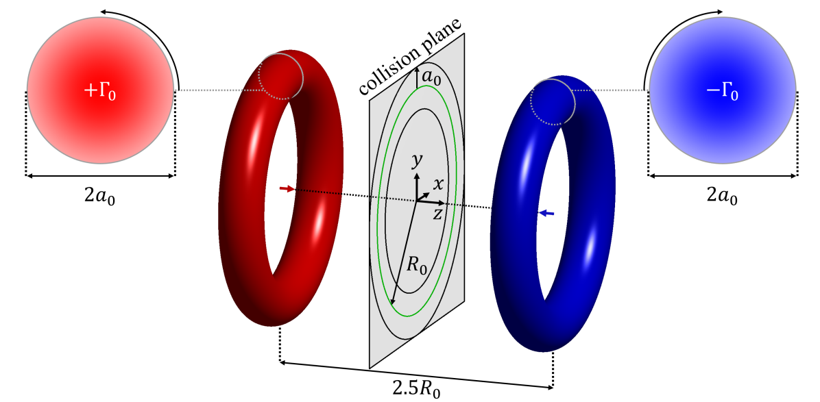
Figure 1: Initial geometry of the flow configuration used to simulate the head-on collision between vortex rings. The shading of the vortex cores reflects their Gaussian vorticity profiles.

As depicted in figure 1, we consider a flow configuration in which the vortex rings are initialized with opposing circulations such that they propagate toward one another along the $z$-axis and meet at the collision plane at $z=0$. The rings are initialized a distance $L_{z}=2.5R_{0}$ apart, which is sufficiently large to mitigate their mutual influence during the most vigorous period of equilibration. Both rings are initialized with Gaussian vorticity distributions (1) such that $Re_{\Gamma_{0}}=$ 4,000 and $\delta_{0}=0.2$. Unless otherwise stated, we use the initial circulation, $\Gamma_{0}=1$, and radius, $R_{0}=1$, of each ring to non-dimensionalize all variables. To excite transition, we randomly perturb the radii of the vortex rings using the first 32 Fourier modes in $\theta$, which are prescribed random phases and uniform magnitudes, $R_{\rm pert}/R_{0}=5\times 10^{-4}$. Consistent with previous tests (Yu et al., 2022), these initial perturbations are sufficiently large to dominate perturbations incurred by discretization errors.

The computational mesh we use has $N_{\rm level}=2$ levels of refinement beyond the base level such that the ratio of the coarsest grid spacing to the finest grid spacing is $\Delta x_{\rm base}/\Delta x_{\rm fine}=4$. Based on preliminary simulations of turbulent vortex rings (Liska & Colonius, 2016) and vortex ring collisions (Yu et al., 2022), we select $a_{0}/\Delta x_{\rm base}=5$ and $\Delta t/\Delta x_{\rm fine}=0.35$ to ensure the flow is well-resolved throughout the simulation. Finally, parameters controlling the spatial and mesh refinement thresholds are chosen as discussed in Appendix A.

2.3 Simulation Integral Metrics

We compute integral metrics (Liska & Colonius, 2016) to track the evolution and fidelity of the simulation. Particularly, we consider metrics representing the momentum, kinetic energy, enstrophy, and helicity of the flow, which are given by $\boldsymbol{I}=\left(I_{x},I_{y},I_{z}\right)$, $K$, $E$, and $H$, respectively. These integrals are formally evaluated on an unbounded domain, but we discretely approximate them using the finite AMR grid as

$$\boldsymbol{I}(t) \approx \int_{V(t)} \boldsymbol{u} dV =\; \;\boldsymbol{I}_{V}(t) -\>\boldsymbol{I}_{\partial V}(t),$$

$$K(t) \approx\frac{1}{2} \int_{V(t)}\lvert \boldsymbol{u}\rvert^{2} dV =\; K_{V}(t) -K_{\partial V}(t),$$ (5)

$$E(t) \approx\frac{1}{2} \int_{V(t)}\lvert \boldsymbol{\omega}\rvert^{2}\; dV \;\,H(t) \approx\int_{V(t)}(\boldsymbol{u}\cdot\boldsymbol{\omega})\;dV,$$ ,

where $V(t)$ is the time-varying AMR grid and $\partial V(t)$ is its boundary.

Due to the favorable decay of vorticity in the far-field, it is convenient to evaluate $\boldsymbol{I}$ and $K$ in terms of the hydrodynamic impulse $\left(\boldsymbol{I}_{V}\right)$ and the vortical kinetic energy $\left(K_{V}\right)$. These integrals and their corresponding correction terms based on the flow at the boundary ($\boldsymbol{I}_{\partial V}$ and $K_{\partial V}$, respectively) are given by

$$\boldsymbol{I}_{V}(t) =\frac{1}{2} \int_{V(t)} (\boldsymbol{x}\times\boldsymbol{\omega})\;dV,\quad \boldsymbol{I}_{\partial V}(t)=\frac{1}{2} \int_{\partial V(t)}\boldsymbol{x}\times(\boldsymbol{n}\times\boldsymbol{u})\;dS,$$ (6a)

$$K_{V}(t) = \int_{V(t)}\boldsymbol{u}\cdot (\boldsymbol{x}\times\boldsymbol{\omega})\;dV,\quad K_{\partial V}(t)= \int_{\partial V(t)}\boldsymbol{x}\cdot\left((\boldsymbol{u}\boldsymbol{u})\cdot\boldsymbol{n}-\frac{1}{2}\lvert\boldsymbol{u}\rvert^{2}\boldsymbol{n}\right)dS,$$ (6b)

where $\boldsymbol{n}$ is the normal vector of $\partial V(t)$ (Wu et al., 2015). Whereas $\boldsymbol{I}_{V}$ converges absolutely, $\boldsymbol{I}$ only converges conditionally on unbounded domains due to the contribution of $\boldsymbol{I}_{\partial V}$. When $V$ is a sphere of infinite radius, the momentum and impulse are directly proportional since $\lvert\boldsymbol{I}_{\partial V}\rvert=\lvert\boldsymbol{I}_{V}\rvert/3$ (Saffman, 1993).

Absent non-conservative external body forces, the hydrodynamic impulse is conserved for incompressible flows on unbounded domains. Since the momentum will also converge on a finite computational grid, its evolution can be used to characterize the influence of the boundary correction term on momentum conservation. The helicity would be conserved in the absence of viscosity, and it is useful for assessing simulation fidelity as the vortex rings initially approach the collision plane since the evolution of the flow is dominated by inviscid effects. These integral metrics initially evaluate to $\boldsymbol{I}(0)=\boldsymbol{I}_{V}(0)=\boldsymbol{0}$ and $H(0)=0$, respectively, due to the spatial symmetries of the initial flow configuration. Correspondingly, their deviations from these initial values reflect the degree to which the symmetries imposing their initial values are broken.

The enstrophy and the kinetic energy provide a more detailed picture of simulation fidelity during transition and turbulent decay, during which viscous dissipation at small scales becomes relevant. For unsteady, incompressible flows on unbounded domains, the dissipation governs the decay rate of kinetic energy and can be expressed in terms of the enstrophy. Comparing these integrals is useful for characterizing (i) the degree to which small-scale features are resolved during peak dissipation and (ii) the flux of kinetic energy out of the finite computational domain (Archer et al., 2008). The relative dissipation error can be quantified using effective Reynolds numbers, which are given by

$$\frac{Re^{\rm eff}_{S}(t)}{Re_{\Gamma_{0}}}=-\frac{\Phi_{S}(t)}{dK/dt},\quad\quad\frac{Re^{\rm eff}_{W}(t)}{Re_{\Gamma_{0}}}=-\frac{\Phi_{W}(t)}{dK/dt},$$ (7)

where $\Phi_{S}$ is the volume-integrated dissipation and $\Phi_{W}=2E/Re_{\Gamma_{0}}$ is its enstrophy-based counterpart (Serrin, 1959). Here, we differentiate $K$ instead of $K_{V}$ when computing the effective Reynolds numbers to prevent amplification of the noise associated with adaptations in the computational domain, to which $K_{V}$ is more sensitive. This is justified since $K$ and $K_{V}$ are nearly identical throughout the present simulations (see figure 2). The ratios in (7) are particularly useful for assessing spatial resolution since the dissipation can vary significantly during transition and turbulent decay. Further, the difference between $Re^{\rm eff}_{S}$ and $Re^{\rm eff}_{W}$ reflects the relative importance of the acceleration of the flow on $\partial V$ through the boundary integral in the Bobyleff-Forsyth formula (Serrin, 1959). Together, the error metrics defined in this section comprehensively characterize the fidelity of the simulation as its flow structures evolve and the computational domain adapts accordingly.

3 Evolution of Integral Metrics and Vortical Structures

3.1 Evolution of Integral Metrics

Figure 2 shows the evolution of the integral metrics from section 2.3 over the course of the simulation. In our subsequent analysis, we reference the various regimes of flow development with respect to the time, $t^{*}=14.77$, at which maximum dissipation is attained. Table 1 qualitatively characterizes the state of the simulation at each reference time we consider for the initial, transitional, and turbulent regimes of the simulation.

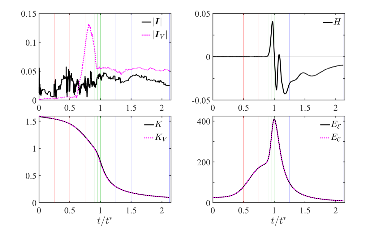
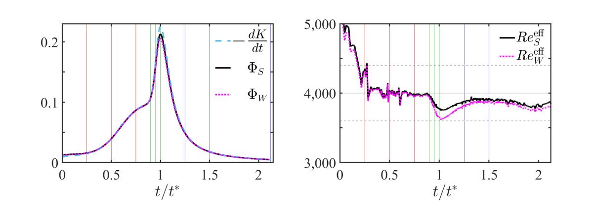
Figure 2: Temporal evolution of the integral metrics defined in section 2.3 over the course of the simulation. The vertical lines correspond to the reference times in table 1 and they are colored accordingly. The horizontal lines in the $Re^{\rm eff}$ panel represent $Re_{\Gamma_{0}}$ (solid) with 10% margins (dashed). The enstrophies $E_{\mathcal{E}}$ and $E_{\mathcal{C}}$ are computed using vorticities located at the edges and centers, respectively, of the computational cells.

Regime of Evolution	$\;\,t/t^{*}$
Post-equilibration vortex rings	0.25
Vortex boundary merger	0.50
Enhanced radial expansion	0.75
Formation of secondary vortices	0.90
Interaction of secondary vortices	0.95
Proliferation of small scales	1.00
Early turbulent decay	1.25
Intermediate turbulent decay	1.50
Late turbulent decay	2.12

Table 1: Reference times used to analyze the initial (red), transitional (green), and turbulent (blue) regimes of the present vortex ring collision, where $t^{*}=14.77$ is the time of maximum dissipation.

The initial evolution of the flow involves a rapid period of equilibration ($t\lesssim 0.25t^{*}$) and the propagation of the equilibrated rings towards the collision plane ($0.25t^{*}\lesssim t\lesssim 0.50t^{*}$). The interaction of the rings accelerates their radial expansion ($0.50t^{*}\lesssim t\lesssim 0.75t^{*}$) and the elliptic instability eventually emerges along the expanding rings ($0.75t^{*}\lesssim t\lesssim 0.90t^{*}$). Subsequently, the flow transitions to turbulence ($0.90t^{*}\lesssim t\lesssim t^{*}$) and rapidly produces small-scale flow structures. Following transition, the flow undergoes turbulent decay for the remainder of the simulation (i.e., for $t\gtrsim t^{*}$). See section 3.2 for visualizations of the flow at the reference times from table 1 in each of these regimes of its evolution.

As the vortex rings initially propagate towards the collision plane ($t\lesssim 0.50t^{*}$) the kinetic energy decays slowly and the enstrophy (and dissipation) are relatively small. The effective Reynolds numbers rapidly adjust to the value of $Re_{\Gamma_{0}}$ during the initial equilibration period ($t\lesssim 0.25t^{*}$) and remain roughly constant as the equilibrated rings approach the collision plane ($0.25t^{*}\lesssim t\lesssim 0.50t^{*}$). During these periods, the impulse and, to a lesser extent, the momentum are initially small and grow relatively slowly. Further, the helicity is well-conserved in this regime since the flow evolves in a nearly inviscid fashion. These results suggest that the symmetries associated with the distribution of momentum and the handedness of the flow are well-preserved in the initial regime of evolution.

As the rings expand radially at the collision plane ($0.50t^{*}\lesssim t\lesssim 0.75t^{*}$) and the elliptic instability emerges ($0.75t^{*}\lesssim t\lesssim 0.90t^{*}$), the kinetic energy decays more rapidly and the dissipation grows. The effective Reynolds numbers remain relatively constant near $Re_{\Gamma_{0}}$, suggesting that the flow is well-resolved, and the symmetry associated with helicity remains well-preserved. However, the impulse magnitude varies more rapidly in time due to the rapid radial expansion of the rings during this period. In following the expanding vortical flow at the collision plane, the adaptations of the domain break the symmetry associated with impulse integral more significantly than during the initial evolution of the rings. The resulting growth in $\lvert\boldsymbol{I}_{V}\rvert$ is primarily attributed to its component in the $z$ direction, along which the domain is compressed as the flow concentrates about the collision plane. This asymmetry not mirrored by the momentum since its integrand is not as significantly influenced by the adaptations of the computational mesh.

As the flow transitions to turbulence ($0.90t^{*}\lesssim t\lesssim t^{*}$), the kinetic energy decays even more rapidly and the dissipation approaches its maximum value. Due to the proliferation of small-scale flow structures during this period, the effective Reynolds numbers drop to their minimum values at $t\approx t^{*}$, when the flow is most difficult to resolve. The increased difference between $Re^{\rm eff}_{S}$ and $Re^{\rm eff}_{W}$ reflects that the acceleration of the flow near $\partial V$ is more relevant at this time. The rapid generation of small-scale flow structures also implies that viscosity plays a more important role in this regime. Correspondingly, the helicity begins to vary in time and, in fact, it reaches its maximum rate of change at the time of peak dissipation. These variations reflect changes in the topological character (e.g., handedness) of the vortex lines in the flow. Whereas the impulse magnitude grows in the radial expansion regime, it decays to a roughly constant value in this transitional regime, consistent with the slowed radial expansion.

During the turbulent decay of the flow ($t\gtrsim t^{*}$), the kinetic energy becomes small and the dissipation decays rapidly, eventually falling below its initial value (at $t\approx 1.62t^{*}$). The dissipation matches the kinetic energy decay rate more closely for this regime than for transition. Further, as the turbulence develops, the effective Reynolds numbers agree well with one another and, to a lesser extent, with $Re_{\Gamma_{0}}$. These features reflect, respectively, that the acceleration near $\partial V$ is less important and that the small-scales are relatively well-resolved, especially with respect to the transitional period. Further, the helicity variations in this turbulent regime eventually slow relative to those observed during transition. The momentum and impulse both remain roughly constant around their values at $t=t^{*}$. The ratio of $\lvert\boldsymbol{I}_{V}\rvert/\lvert\boldsymbol{I}\rvert$ is also roughly constant ($\approx 1.48$ on average) and similar to the value (1.5) associated with a spherical domain of infinite radius. Whereas the $z$ component dominates the impulse magnitude during the radial expansion of the rings, all impulse components have similar magnitudes in this turbulent regime.

The evolution of the integral metrics characterizes the various regimes of the flow and supports the fidelity of our simulation. After equilibration, the maximum errors in $Re^{\rm eff}_{S}$ and $Re^{\rm eff}_{W}$ over the remainder of the simulation, both of which occur around $t\approx t^{*}$, are roughly 6.5% and 9.5% of $Re_{\Gamma_{0}}$, respectively. These dissipation errors are similar to those of a previous simulation of a single vortex ring at $Re_{\Gamma_{0}}=$ 7,500 (Archer et al., 2008). Further, these errors are considerably smaller during the approach and radial expansion of the rings and, to a lesser extent, during turbulent decay. These relatively small dissipation errors suggest that the small-scale flow structures remain reasonably well-resolved throughout the entire simulation. The symmetries associated with the handedness and momentum distribution of the flow also remain well-preserved in the appropriate regimes of the simulation. For example, the helicity is well-conserved during the nearly-inviscid evolution of the vortex rings and its subsequent variations are relatively small in magnitude. Similarly, the variations in impulse and momentum magnitudes remain less than 5% of the impulse associated with each vortex ring in isolation throughout the simulation. Altogether, these results suggest that our simulations are of sufficiently high fidelity to probe the mechanisms underlying transition and turbulent decay.

3.2 Evolution of Vortical Flow Structures

For the present simulation, we identify vortices using the $\Omega_{r}$ criterion (Liu et al., 2019a) with a numerical threshold of $\varepsilon_{\rm vort}$ = 0.04. This criterion provides connections to the triple decomposition of the VGT and the structure of local streamlines. Due to the well-preserved symmetries of the flow, the global spatial mean of the vorticity tensor is nearly zero and, hence, the $\Omega_{r}$ criterion is nearly objective (Liu et al., 2019c) for the present simulation. We specifically visualize the flow using $\Omega_{r}=0.52$ and $\Omega_{r}=0.93$ to investigate the structures of the vortex boundaries and the vortex cores, respectively. We color these structures using ${\rm cos}\,\theta^{*}$, where $\theta^{*}$ is the angle between the $z^{*}$-axis and the $z$-axis. This color scheme enables the identification of antiparallel vortices along the $z$-axis, which play an important role in mediating transition and generating small-scale flow structures in the present vortex ring collision. In figure 3, we visualize the vortical structures in the flow at each reference time from table 1.

During the initial evolution of the flow, the equilibrated vortex rings approach the collision plane and expand radially due to their mutual interaction. In this regime, the thinning of the vortex boundaries and cores illustrates the mechanisms driving the shift from a rigid-rotation-dominated regime to a shearing-dominated regime. Further, the visualizations at $t=0.75t^{*}$ reveal the emergence of the (shortwave) elliptic instability, which is consistent with previous vortex ring collision simulations in similar parameter regimes (McKeown et al., 2020; Mishra et al., 2021).

The transitional regime of the flow is marked by the development of secondary vortex filaments and the subsequent generation of small-scale vortical flow structures. At $t=0.90t^{*}$, the visualizations show the development of secondary vortical structures around the circumference of the collision. These structures consist of antiparallel vortex filament pairs that arise in regions where the elliptic instability drives local interactions between the rings. This behavior supports the notion that the elliptic instability mediates the initial transition of the rings prior to the development of secondary vortical structures. These antiparallel secondary filaments become increasingly densely-packed as transition progresses and they mediate the proliferation of small-scale vortical flow structures, e.g., as observed at $t=t^{*}$. These observations are consistent with the initial stages of the iterative cascade pathway, which is driven by subsequent generations of antiparallel vortex filaments (McKeown et al., 2020).

During the turbulent decay of the flow, the geometric features of the vortex boundaries remain similar at each reference time. However, as energy is dissipated, the smallest-scale vortices are progressively destroyed and the vortical flow structures grow larger in time. The structures of the vortex cores and boundaries provide further evidence that the interactions between the secondary vortex filaments help mediate the evolution of the turbulent flow. The vortex boundaries also show the formation and ejection of vortex rings from the turbulent cloud resulting from the collision. These ejections, which are a hallmark of the Crow instability, often occur in regions where antiparallel vortex filaments interact and are of similar size to those filaments. This observation provides further evidence of the interplay between the elliptic and Crow instabilities driven by interacting vortex filaments around the turbulent cloud (Mishra et al., 2021; Ostilla-Mónico et al., 2021). In what follows, we develop machinery to probe these mechanisms in the context of features of the velocity gradients, with a particular emphasis on characterizing the action of the elliptic instability among other mechanisms.

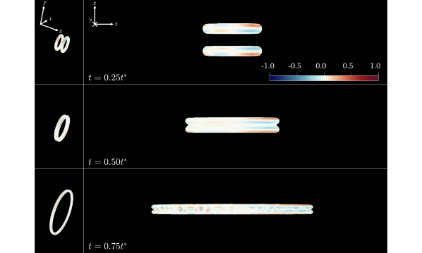
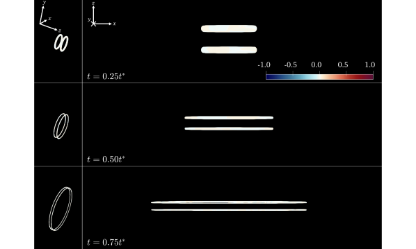
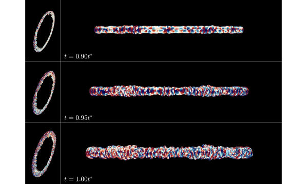
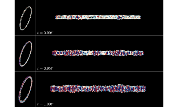
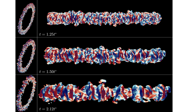
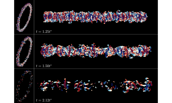
Figure 3: Visualizations of the vortex boundaries ($\Omega_{r}=0.52$, left side) and vortex cores ($\Omega_{r}=0.93$, right side), colored by ${\rm cos}\,\theta^{*}$, for each reference time from table 1. A movie depicting the evolution of the vortex boundaries from the auxiliary viewpoint (leftmost column) is provided as supplementary material.

4 Partitioning of Velocity Gradients

Here, we investigate the partitioning of the velocity gradients to characterize the evolution of the flow in the context of the fundamental modes of deformation. We first consider volumetric weighted averages of the relative contributions of various constituents of $\boldsymbol{\tilde{A}}$ to the strength of the velocity gradients. These averages may be expressed as

$$\big{\langle}{\xi}\big{\rangle}_{\mkern-3.0muA^{2}}=\frac{\int_{V(t)}A^{2}\xi dV}{\int_{V(t)}A^{2}\;\,dV},$$ (8)

where $\xi\in\{\tilde{S}^{2},\tilde{W}^{2}\}$ for the Cauchy-Stokes decomposition and $\xi\in\{\dot{\epsilon}^{2},\dot{\gamma}^{2},\dot{\varphi}^{2},2\boldsymbol{\dot{\varphi}}\mkern-5.0mu:\mkern-5.0mu\boldsymbol{\dot{\gamma}}\}$ for the triple decomposition. Here, we have used that the Frobenius inner product (denoted by $\boldsymbol{:}$) of a symmetric tensor with an antisymmetric tensor is zero and that $\dot{\gamma}^{2}_{\rule{0.0pt}{-6.02777pt}\mkern-2.0muW}=\dot{\gamma}^{2}_{\rule{0.0pt}{-6.02777pt}\mkern-2.0muS}=\dot{\gamma}^{2}/2$. The shear-rotation correlation term, $2\boldsymbol{\dot{\varphi}}\mkern-5.0mu:\mkern-5.0mu\boldsymbol{\dot{\gamma}}=2\dot{\varphi}_{z^{*}}\dot{\gamma}_{z^{*}}>0$, reflects the presence of shearing in the plane of rigid rotation. All of the relative contributions discussed are unitarily invariant and, thus, they apply to both the principal coordinates and the global coordinates. Figure 4 shows how these relative contributions evolve during the simulation for both decompositions of $\boldsymbol{\tilde{A}}$.

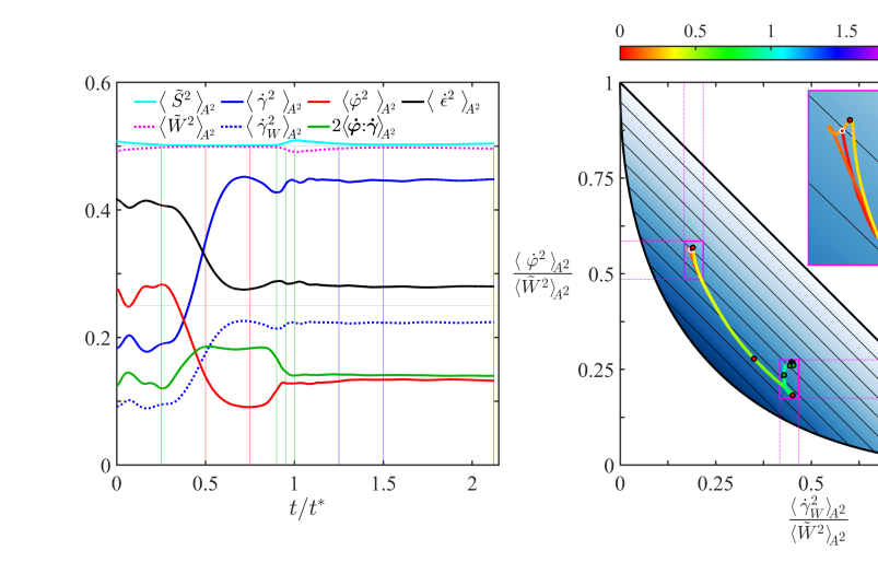
Figure 4: Relative contributions of the constituents of the Cauchy-Stokes decomposition and the triple decomposition to $A^{2}$. The vertical lines correspond to the reference times in table 1 and they are colored accordingly.

Consistent with the equivalence of $\Phi_{S}$ and $\Phi_{W}$ for incompressible flows on unbounded domains (Serrin, 1959), $\big{\langle}{\tilde{S}^{2}}\big{\rangle}_{\mkern-3.0muA^{2}}\approx\big{\langle}{\tilde{W}^{2}}\big{\rangle}_{\mkern-3.0muA^{2}}\approx 0.50$ for the present simulations. The largest deviations from this balance occur during equilibration ($t\lesssim 0.25t^{*}$) and around the time of peak dissipation ($t\approx t^{*}$). These deviations are consistent with the behavior of the effective Reynolds numbers in figure 2 and their smallness further validates the ability of the finite computational grid to approximate a formally unbounded flow. However, since $\big{\langle}{\tilde{S}^{2}}\big{\rangle}_{\mkern-3.0muA^{2}}$ and $\big{\langle}{\tilde{W}^{2}}\big{\rangle}_{\mkern-3.0muA^{2}}$ remain relatively constant throughout the simulation, they provide limited information about the nature of the velocity gradients as the flow progresses through its initial, transitional, and turbulent regimes.

Compared to the constituents of the Cauchy-Stokes decomposition, the constituents of the triple decomposition show more pronounced variations associated with the different regimes of evolution. For the initial Gaussian vorticity profiles, the contribution of rigid rotation to the enstrophy dominates the contribution of antisymmetric shearing. During equilibration ($t\lesssim 0.25t^{*}$), the fluctuations in all contributions of the triple decomposition constituents reflect the redistribution of velocity gradients in the cores of the vortex rings. As the equilibrated rings approach the collision plane and spread ($0.25t^{*}\lesssim t\lesssim 0.75t^{*}$), $\big{\langle}{\dot{\epsilon}^{2}}\big{\rangle}_{\mkern-3.0muA^{2}}$ and $\big{\langle}{\dot{\varphi}^{2}}\big{\rangle}_{\mkern-3.0muA^{2}}$ decrease and $\big{\langle}{\dot{\gamma}^{2}}\big{\rangle}_{\mkern-3.0muA^{2}}$ and $2\big{\langle}{\boldsymbol{\dot{\varphi}}\mkern-5.0mu:\mkern-5.0mu\boldsymbol{\dot{\gamma}}}\big{\rangle}_{\mkern-3.0muA^{2}}$ increase. As the elliptic instability emerges, these contributions level off in a regime where antisymmetric shearing dominates rigid rotation and shear-rotation correlations are enhanced. The subsequent development of the elliptic instability ($0.75t^{*}\lesssim t\lesssim 0.90t^{*}$) is marked by slight rebounds in the contributions of $\big{\langle}{\dot{\varphi}^{2}}\big{\rangle}_{\mkern-3.0muA^{2}}$ and $\big{\langle}{\dot{\gamma}^{2}}\big{\rangle}_{\mkern-3.0muA^{2}}$. The transition to turbulence ($0.90t^{*}\lesssim t\lesssim t^{*}$), which is associated with the generation of small scales and enhanced dissipation, is marked by a decrease in the contribution of $2\big{\langle}{\boldsymbol{\dot{\varphi}}\mkern-5.0mu:\mkern-5.0mu\boldsymbol{\dot{\gamma}}}\big{\rangle}_{\mkern-3.0muA^{2}}$.

Remarkably, even though the flow is not stationary during turbulent decay, the relative contributions of the constituents of the triple decomposition to the strength of the velocity gradients remain roughly constant after transition. As summarized in table 2, the “equilibrium” relative contributions of each constituent in this regime are similar to those computed by Das & Girimaji (2020b) for forced isotropic turbulence at high Taylor Reynolds numbers. This agreement is particularly striking in that the present flow is not stationary and it suggests that the velocity gradient partitioning may reflect a common balance in unbounded, incompressible turbulence with appropriate symmetries. In this balance, shearing has the largest contribution to the velocity gradients and rigid rotation has the smallest contribution.

Constituent	$\big{\langle}{\dot{\epsilon}^{2}}\big{\rangle}_{\mkern-3.0muA^{2}}$	$\big{\langle}{\dot{\gamma}^{2}}\big{\rangle}_{\mkern-3.0muA^{2}}$	$\big{\langle}{\dot{\varphi}^{2}}\big{\rangle}_{\mkern-3.0muA^{2}}$	$2\big{\langle}{\boldsymbol{\dot{\varphi}}\mkern-5.0mu:\mkern-5.0mu\boldsymbol{\dot{\gamma}}}\big{\rangle}_{\mkern-3.0muA^{2}}$
Vortex Ring Collision	28.0 %	44.6 %	13.3 %	14.1 %
Forced Isotropic Turbulence (Das & Girimaji, 2020b)	24   %	52   %	11   %	13   %

Table 2: Comparison of the equilibrium partitioning of the velocity gradients for the present vortex ring collision with the partitioning computed for forced isotropic turbulence (Das & Girimaji, 2020b). Here, the equilibrium partitioning is computed as the mean over the turbulent decay regime ($t\gtrsim t^{*}$) and it is insensitive to the length of the averaging interval.

Beyond the strength of velocity gradients, it is also useful to examine the interplay between the modes of deformation in the context of vortical flow structures. Here, we introduce a new phase space defined by the relative contributions of $\big{\langle}{\dot{\gamma}^{2}_{\rule{0.0pt}{-6.02777pt}\mkern-2.0muW}}\big{\rangle}_{\mkern-3.0muA^{2}}$, $\big{\langle}{\dot{\varphi}^{2}}\big{\rangle}_{\mkern-3.0muA^{2}}$, and (implicitly) $2\big{\langle}{\boldsymbol{\dot{\varphi}}\mkern-5.0mu:\mkern-5.0mu\boldsymbol{\dot{\gamma}}}\big{\rangle}_{\mkern-3.0muA^{2}}$ to $\big{\langle}{\tilde{W}^{2}}\big{\rangle}_{\mkern-3.0muA^{2}}$. The upper bound of this phase space is found by maximizing $\big{\langle}{\dot{\varphi}^{2}}\big{\rangle}_{\mkern-3.0muA^{2}}/\big{\langle}{\tilde{W}^{2}}\big{\rangle}_{\mkern-3.0muA^{2}}$, which occurs when $2\big{\langle}{\boldsymbol{\dot{\varphi}}\mkern-5.0mu:\mkern-5.0mu\boldsymbol{\dot{\gamma}}}\big{\rangle}_{\mkern-3.0muA^{2}}/\big{\langle}{\tilde{W}^{2}}\big{\rangle}_{\mkern-3.0muA^{2}}=0$. The bottom boundary is found by minimizing $\big{\langle}{\dot{\varphi}^{2}}\big{\rangle}_{\mkern-3.0muA^{2}}/\big{\langle}{\tilde{W}^{2}}\big{\rangle}_{\mkern-3.0muA^{2}}$, which occurs when $2\big{\langle}{\boldsymbol{\dot{\varphi}}\mkern-5.0mu:\mkern-5.0mu\boldsymbol{\dot{\gamma}}}\big{\rangle}_{\mkern-3.0muA^{2}}/\big{\langle}{\tilde{W}^{2}}\big{\rangle}_{\mkern-3.0muA^{2}}=2\big{\langle}{\dot{\varphi}^{2}}\big{\rangle}_{\mkern-3.0muA^{2}}\big{\langle}{\dot{\gamma}^{2}_{\rule{0.0pt}{-6.02777pt}\mkern-2.0muW}}\big{\rangle}_{\mkern-3.0muA^{2}}/\big{\langle}{\tilde{W}^{2}}\big{\rangle}_{\mkern-3.0muA^{2}}$. Correspondingly, these boundaries may be expressed as

$$\Bigg{(}1 - \sqrt{\frac{\big{\langle}{\dot{\gamma}^{2}_{\rule{0.0pt}{-6.02777pt}\mkern-2.0muW}}\big{\rangle}_{\mkern-3.0muA^{2}}}{\big{\langle}{\tilde{W}^{2}}\big{\rangle}_{\mkern-3.0muA^{2}}}} \Bigg{)}^{2} \leq \;\,\frac{\big{\langle}{\dot{\varphi}^{2}}\big{\rangle}_{\mkern-3.0muA^{2}}}{\big{\langle}{\tilde{W}^{2}}\big{\rangle}_{\mkern-3.0muA^{2}}} \leq 1 -\frac{\big{\langle}{\dot{\gamma}^{2}_{\rule{0.0pt}{-6.02777pt}\mkern-2.0muW}}\big{\rangle}_{\mkern-3.0muA^{2}}}{\big{\langle}{\tilde{W}^{2}}\big{\rangle}_{\mkern-3.0muA^{2}}},$$ (9)

$$\Updownarrow \Updownarrow$$

$$-2\Bigg{(}\frac{\big{\langle}{\dot{\gamma}^{2}_{\rule{0.0pt}{-6.02777pt}\mkern-2.0muW}}\big{\rangle}_{\mkern-3.0muA^{2}}}{\big{\langle}{\tilde{W}^{2}}\big{\rangle}_{\mkern-3.0muA^{2}}} - \sqrt{\frac{\big{\langle}{\dot{\gamma}^{2}_{\rule{0.0pt}{-6.02777pt}\mkern-2.0muW}}\big{\rangle}_{\mkern-3.0muA^{2}}}{\big{\langle}{\tilde{W}^{2}}\big{\rangle}_{\mkern-3.0muA^{2}}}} \Bigg{)} \geq \frac{2\big{\langle}{\boldsymbol{\dot{\varphi}}\mkern-5.0mu:\mkern-5.0mu\boldsymbol{\dot{\gamma}}}\big{\rangle}_{\mkern-3.0muA^{2}}}{\big{\langle}{\tilde{W}^{2}}\big{\rangle}_{\mkern-3.0muA^{2}}} \geq \;0,$$ (10)

highlighting that lower and upper bounds of the rigid rotation contribution correspond to the upper and lower bounds, respectively, of the shear-rotation correlation contribution. The maximum value of $2\big{\langle}{\boldsymbol{\dot{\varphi}}\mkern-5.0mu:\mkern-5.0mu\boldsymbol{\dot{\gamma}}}\big{\rangle}_{\mkern-3.0muA^{2}}/\big{\langle}{\tilde{W}^{2}}\big{\rangle}_{\mkern-3.0muA^{2}}$ varies along the lower boundary of this phase space to ensure that the relative contributions sum to unity. The global maximum occurs when $2\boldsymbol{\dot{\varphi}}\mkern-5.0mu:\mkern-5.0mu\boldsymbol{\dot{\gamma}}/\tilde{W}^{2}=0.5$ or, equivalently, $\dot{\varphi}^{2}/\tilde{W}^{2}=\dot{\gamma}^{2}_{\rule{0.0pt}{-6.02777pt}\mkern-2.0muW}/\tilde{W}^{2}=0.25$ at all points, which corresponds to the (pointwise) maximum of $2\boldsymbol{\dot{\varphi}}\mkern-5.0mu:\mkern-5.0mu\boldsymbol{\dot{\gamma}}=(\sqrt{2}+1)^{-1}$ reported by Das & Girimaji (2020b). This maximum corresponds to local streamlines (in the principal frame) for which shearing occurs exclusively in the plane of rigid rotation.

Figure 5: Shear-rotation phase space trajectory of the flow, highlighting the evolution during equilibration (left inset) and transition and turbulent decay (right inset). The contours represent increments of 0.05 in the color scale. The white circle marks the initial condition and the black circles mark the reference times from table 1 and their fill colors are specified accordingly.

Figure 5 depicts the trajectory of the flow in this shear-rotation phase space and elucidates how the relationships between the constituents of enstrophy associated with the triple decomposition evolve in time. Following rapid variations during equilibration, the trajectory returns to a position in phase space similar to that of the initial condition at $t\approx 0.25t^{*}$. The trajectory then undergoes a shift across the phase space as the equilibrated rings approach the collision plane and spread radially ($0.25t^{*}\lesssim t\lesssim 0.75t^{*}$). This shift from a rigid-rotation-dominated regime to a shearing-dominated regime is associated with an enhanced contribution from $2\big{\langle}{\boldsymbol{\dot{\varphi}}\mkern-5.0mu:\mkern-5.0mu\boldsymbol{\dot{\gamma}}}\big{\rangle}_{\mkern-3.0muA^{2}}/\big{\langle}{\tilde{W}^{2}}\big{\rangle}_{\mkern-3.0muA^{2}}$. The development of the elliptic instability ($0.75t^{*}\lesssim t\lesssim 0.90t^{*}$) and transition ($0.90t^{*}\lesssim t\lesssim t^{*}$) are associated with a shift in the direction of the trajectory towards smaller contributions of $2\big{\langle}{\boldsymbol{\dot{\varphi}}\mkern-5.0mu:\mkern-5.0mu\boldsymbol{\dot{\gamma}}}\big{\rangle}_{\mkern-3.0muA^{2}}/\big{\langle}{\tilde{W}^{2}}\big{\rangle}_{\mkern-3.0muA^{2}}$. During turbulent decay ($t\gtrsim t^{*}$), the trajectory remains roughly fixed in the phase space and very close to its position at $t=t^{*}$.

Considering this phase space trajectory in the context of the dissipation (see figure 2) reveals that, while the initial growth in dissipation is associated with enhanced shear-rotation correlations, its subsequent enhancement during transition is associated with a reduction in shear-rotation correlations. In Appendix B, we reexamine the visualizations from figure 3 through the lens of the shear-rotation correlations in the flow to highlight their relationship to the vortical flow structures. In section 5, we interpret the effects of these shear-rotation correlations through the lens of the elliptic instability and related mechanisms by introducing a new, related phase space based on local streamline geometry.

5 Statistical Geometry of Local Streamlines

5.1 Phase Space Transformations

Intuitively, the processes leading to turbulence in the present simulation can be understood through the lens of the elliptic instability, which is associated with the resonance of the vortical flow with the underlying strain field and acts to break up elliptic streamlines. Consistent with this picture, we introduce a new geometry-based phase space that captures local flow features that (i) are conducive to the elliptic instability and (ii) characterize its action.

To address (i), we consider the angle, $\theta_{\omega}$, between the vorticity vectors associated with antisymmetric shearing and rigid rotation, which is given by

$$\theta_{\omega}={\rm cos}^{-1}\left(\sqrt{\frac{\left(\boldsymbol{\dot{\varphi}}\mkern-5.0mu:\mkern-5.0mu\boldsymbol{\dot{\gamma}}\right)^{2}}{\dot{\varphi}^{2}\dot{\gamma}^{2}_{\rule{0.0pt}{-6.02777pt}\mkern-2.0muW}}}\right).$$ (11)

Our focus on shear straining is consistent with the classical models of strained vortices used to characterize the elliptic instability (Kerswell, 2002). Since decreasing $\theta_{\omega}$ corresponds to increasing the alignment between shearing and rigid rotation, it can be associated with conditions conducive to the elliptic instability.

To address (ii), we consider the aspect ratio, $\zeta$, of the elliptic component of (rotational) local streamlines in the plane of rigid rotation, which is given by

$$\zeta=\sqrt{1-e^{2}}=\sqrt{\frac{\dot{\varphi}^{2}}{\dot{\varphi}^{2}+2\boldsymbol{\dot{\varphi}}\mkern-5.0mu:\mkern-5.0mu\boldsymbol{\dot{\gamma}}}},$$ (12)

where $e$ represents the eccentricity of an ellipse with aspect ratio $\zeta$. This aspect ratio completely characterizes the scale-invariant geometry of the local streamlines in the plane of rigid rotation. As such, it can be used alongside $\theta_{\omega}$ to characterize the action of the elliptic instability by identifying how alignment between shearing and rigid rotation affects local streamline geometry.

These new shear-rotation and geometry-based phase spaces can be understood through nonlinear transformations of the $q_{\rule{0.0pt}{4.82224pt}\mkern-3.0muA}-\,r_{\rule{0.0pt}{4.82224pt}\mkern-4.0muA}$ phase space. The transformations we derive express the relative contributions of the triple decomposition to the velocity gradients using $q_{\rule{0.0pt}{4.82224pt}\mkern-3.0muA}$ and $r_{\rule{0.0pt}{4.82224pt}\mkern-4.0muA}$, and they represent the inverse transformations to those presented by Das & Girimaji (2020b). However, an additional parameter, $\theta_{\omega}$, is generally required to evaluate our transformations. This extra parameter demonstrates that the invariants of $\boldsymbol{\tilde{A}}$ alone cannot generally characterize the relative contributions of the constituents of the triple decomposition to the velocity gradients.

For rotational local streamlines, the transformations are given by

$$\begin{split}\dot{\epsilon}^{2}&=\frac{\left(-3\cdot 2^{2/3}q_{\rule{0.0pt}{4.82224pt}\mkern-3.0muA}+3^{2/3}\left(2\sqrt{3\Delta}+9\lvert r_{\rule{0.0pt}{4.82224pt}\mkern-4.0muA}\rvert\right)^{2/3}\right)^{2}}{6^{5/3}\left(2\sqrt{3\Delta}+9\lvert r_{\rule{0.0pt}{4.82224pt}\mkern-4.0muA}\rvert\right)^{2/3}},\quad\quad\dot{\gamma}^{2}=2\dot{\gamma}^{2}_{\rule{0.0pt}{-6.02777pt}\mkern-2.0muW}=1-2\dot{\epsilon}^{2}-2q_{\rule{0.0pt}{4.82224pt}\mkern-3.0muA}\;,\\ \dot{\varphi}^{2}&=\left(-\sqrt{\dot{\gamma}^{2}_{\rule{0.0pt}{-6.02777pt}\mkern-2.0muW}}{\rm cos}\theta_{\rm\omega}+\sqrt{1-\dot{\epsilon}^{2}-\dot{\gamma}^{2}_{\rule{0.0pt}{-6.02777pt}\mkern-2.0muW}\left(2-{\rm cos}^{2}\theta_{\omega}\right)}\right)^{2},\quad 2\boldsymbol{\dot{\varphi}}\mkern-5.0mu:\mkern-5.0mu\boldsymbol{\dot{\gamma}}=2\sqrt{\dot{\varphi}^{2}\dot{\gamma}^{2}_{\rule{0.0pt}{-6.02777pt}\mkern-2.0muW}}{\rm cos}\theta_{\omega},\end{split}$$ (13)

where $\Delta=q_{\rule{0.0pt}{4.82224pt}\mkern-3.0muA}{}^{3}+\frac{27}{4}r_{\rule{0.0pt}{4.82224pt}\mkern-4.0muA}{}^{2}$ is (proportional to) the discriminant of the characteristic equation of $\boldsymbol{\tilde{A}}$. In this case, $\dot{\epsilon}^{2}$ and $\dot{\gamma}^{2}$ can be determined directly from $q_{\rule{0.0pt}{4.82224pt}\mkern-3.0muA}$ and $r_{\rule{0.0pt}{4.82224pt}\mkern-4.0muA}$ and $\dot{\varphi}^{2}$, $2\boldsymbol{\dot{\varphi}}\mkern-5.0mu:\mkern-5.0mu\boldsymbol{\dot{\gamma}}$, and $\zeta$ can be determined if $\theta_{\omega}$ is known. For non-rotational local streamlines, the transformations are given by

$$\dot{\epsilon}^{2}=-2q_{\rule{0.0pt}{4.82224pt}\mkern-3.0muA},\quad\dot{\gamma}^{2}=1-\dot{\epsilon}^{2},\quad\dot{\varphi}^{2}=0,$$ (14)

which can be determined directly from a single parameter, $q_{\rule{0.0pt}{4.82224pt}\mkern-3.0muA}$. The rotational and non-rotational transformations are continuous with one another at their boundary ($\Delta=0$) and they are both symmetric about the $q_{\rule{0.0pt}{4.82224pt}\mkern-3.0muA}$-axis. However, the aspect ratio is only well-defined for $\Delta>0$, consistent with our focus on rotational local streamlines in the context of the elliptic instability.

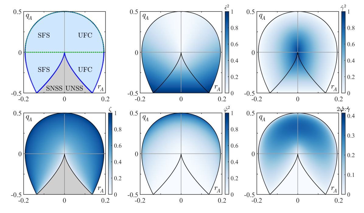
Figure 6: The $q_{\rule{0.0pt}{4.82224pt}\mkern-3.0muA}-\,r_{\rule{0.0pt}{4.82224pt}\mkern-4.0muA}$ phase space (top left) and the variations in $\dot{\epsilon}^{2}$, $\dot{\gamma}^{2}$, $\dot{\varphi}^{2}$, $2\boldsymbol{\dot{\varphi}}\mkern-5.0mu:\mkern-5.0mu\boldsymbol{\dot{\gamma}}$, and $\zeta$ in this space when $\theta_{\omega}=43.57^{\circ}$ is held constant. The top left panel shows the boundaries corresponding to the symmetry-based (dotted green) and the vorticity-based (solid blue) vortex criteria (see section 1.2). It also labels the four classes of non-degenerate local streamline topologies: stable-focus-stretching (SFS), unstable-focus-compression (UFC), stable-node-saddle-saddle (SNSS), and unstable-node-saddle-saddle (UNSS).

In figure 6, we illustrate how $\dot{\epsilon}^{2}$, $\dot{\gamma}^{2}$, $\dot{\varphi}^{2}$, $2\boldsymbol{\dot{\varphi}}\mkern-5.0mu:\mkern-5.0mu\boldsymbol{\dot{\gamma}}$, and $\zeta$ vary within the $q_{\rule{0.0pt}{4.82224pt}\mkern-3.0muA}-\,r_{\rule{0.0pt}{4.82224pt}\mkern-4.0muA}$ phase space. In this phase space, the rotational geometries are externally bounded by $3\sqrt{3}\lvert r_{\rule{0.0pt}{4.82224pt}\mkern-4.0muA}\rvert=(1+q_{\rule{0.0pt}{4.82224pt}\mkern-3.0muA})(1-2q_{\rule{0.0pt}{4.82224pt}\mkern-3.0muA})^{1/2}$ and the non-rotational geometries are externally bounded by $q_{\rule{0.0pt}{4.82224pt}\mkern-3.0muA}=-\frac{1}{2}$. For the rotational geometries, we display $\dot{\varphi}^{2}$, $2\boldsymbol{\dot{\varphi}}\mkern-5.0mu:\mkern-5.0mu\boldsymbol{\dot{\gamma}}$, and $\zeta$ for $\theta_{\omega}=43.57^{\circ}$, which corresponds to its mean value at $t=1.25t^{*}$ (see figure 8) and approximates the equilibrium value during turbulent decay. We document how each of these quantities varies with $\theta_{\omega}$ in the $q_{\rule{0.0pt}{4.82224pt}\mkern-3.0muA}-\,r_{\rule{0.0pt}{4.82224pt}\mkern-4.0muA}$ phase space in Appendix C.

Figure 6 shows that, generically, the contribution of pure shearing ($\dot{\gamma}^{2}$) tends to dominate the velocity gradients near the origin of the $q_{\rule{0.0pt}{4.82224pt}\mkern-3.0muA}-\;r_{\rule{0.0pt}{4.82224pt}\mkern-4.0muA}$ plane. The contribution of normal straining ($\dot{\epsilon}^{2}$) grows large when the velocity gradients are dominated by the strain rate tensor. By contrast, for rotational geometries, the contribution of rigid rotation ($\dot{\varphi}^{2}$) grows large near the external boundary in regions where the vorticity tensor dominates. The contribution of shear-rotation correlations ($2\boldsymbol{\dot{\varphi}}\mkern-5.0mu:\mkern-5.0mu\boldsymbol{\dot{\gamma}}$) grows largest in the intermediate region of the phase space and it decays near the discriminant line and the external boundary. The aspect ratio $\zeta$ is unity along the external boundary and it decays to zero at the discriminant line.

The elliptic instability, which is relevant in strained vortical flows, is expected to be most active for an intermediate range of aspect ratios. Further, vortex stretching and squeezing, which are known to play important roles in the turbulent cascade, can most readily be associated with the SFS and UFC streamline topologies, respectively (Lopez & Bulbeck, 1993). Using the corresponding regions in the $q_{\rule{0.0pt}{4.82224pt}\mkern-3.0muA}-\;r_{\rule{0.0pt}{4.82224pt}\mkern-4.0muA}$ plane, the transformations in figure 6 suggest that the interplay between shearing and rotation is pertinent to these fundamental turbulent processes. They thus suggest that, among other mechanisms, the elliptic instability has the potential to play a role in mediating these processes. To further probe these relationships, in section 5.2 we analyze how the distributions of the velocity gradients in the $q_{\rule{0.0pt}{4.82224pt}\mkern-3.0muA}-\,r_{\rule{0.0pt}{4.82224pt}\mkern-4.0muA}$, shear-rotation, and $\zeta-\theta_{\omega}$ phase spaces evolve during the simulation.

5.2 Phase Space Distributions

The joint probability density functions (pdfs) of the normalized velocity gradients in the phase spaces we investigate encode information about the local streamline geometries. Although these phase spaces are related to one another, the choice of phase space plays an important role in interpreting the statistical distributions of the flow. In the $q_{\rule{0.0pt}{4.82224pt}\mkern-3.0muA}-\,r_{\rule{0.0pt}{4.82224pt}\mkern-4.0muA}$ phase space, incompressible turbulent flows often follow a near-universal teardrop-shaped distribution about the origin (Das & Girimaji, 2019, 2020a). The shear-rotation phase space highlights the distribution of rotational streamline geometries and it characterizes the interplay of rigid rotation and antisymmetric shearing. The $\zeta-\theta_{\omega}$ phase space also considers rotational streamline geometries and it characterizes the flow through the lens of geometric features of local streamlines that are associated with the elliptic instability.

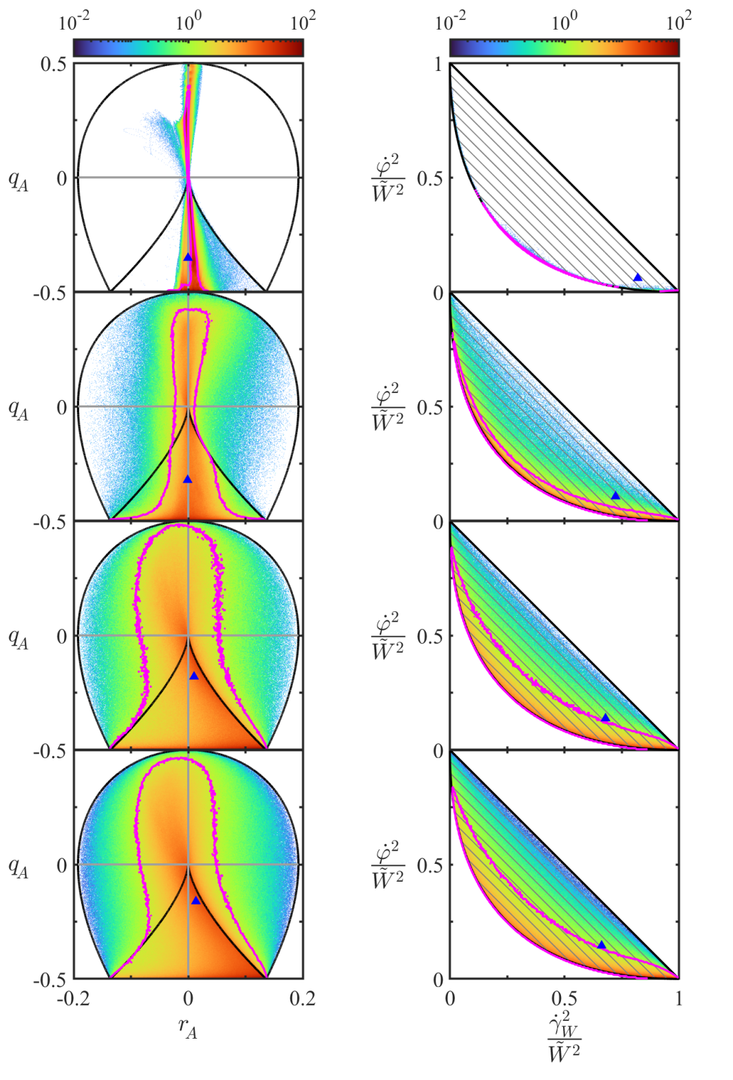
Figure 7: Joint pdfs of the velocity gradients satisfying $A^{2}/{\rm max}(A^{2})\geq 0.1\%$ in the $q_{\rule{0.0pt}{4.82224pt}\mkern-3.0muA}-\,r_{\rule{0.0pt}{4.82224pt}\mkern-4.0muA}$ phase space (left) and $W^{2}/{\rm max}(W^{2})\geq 0.1\%$ in the shear-rotation phase space (right) at times $t=0.75t^{*}$, $0.90t^{*}$, $1.00t^{*}$, and $1.25t^{*}$ (from top to bottom). The blue triangles represent the centroids of the distributions and the magenta contours represent the pdf levels for which 90% of the flow (by volume) resides at higher pdf levels. These contours are smoothed by using coarser pdf bins to ensure that they roughly enclose the regions with higher pdf levels.

Figure 7 shows the $q_{\rule{0.0pt}{4.82224pt}\mkern-3.0muA}-\,r_{\rule{0.0pt}{4.82224pt}\mkern-4.0muA}$ and the shear-rotation phase space distributions at reference times, selected from table 1, that pertain to the development of the elliptic instability, transition, and turbulent decay. As the elliptic instability emerges ($t\approx 0.75t^{*}$), the velocity gradients are concentrated near the $q_{\rule{0.0pt}{4.82224pt}\mkern-3.0muA}$-axis. Since $2\big{\langle}{\boldsymbol{\dot{\varphi}}\mkern-5.0mu:\mkern-5.0mu\boldsymbol{\dot{\gamma}}}\big{\rangle}_{\mkern-3.0muA^{2}}$ is relatively large around this time, the rotational regions of the flow are concentrated near the bottom boundary of the shear-rotation phase space, particularly near the location where $2\big{\langle}{\boldsymbol{\dot{\varphi}}\mkern-5.0mu:\mkern-5.0mu\boldsymbol{\dot{\gamma}}}\big{\rangle}_{\mkern-3.0muA^{2}}$ is maximized.

As the flow transitions ($t\approx 0.90t^{*}$), the distribution remains centered about the $q_{\rule{0.0pt}{4.82224pt}\mkern-3.0muA}$-axis but it expands towards larger $\lvert r_{\rule{0.0pt}{4.82224pt}\mkern-4.0muA}\rvert$ as it begins to fill the $q_{\rule{0.0pt}{4.82224pt}\mkern-3.0muA}-\,r_{\rule{0.0pt}{4.82224pt}\mkern-4.0muA}$ phase space. Similarly, the pdf in the shear-rotation phase space begins extending away from the bottom boundary of the phase space, although its bulk remains concentrated at the boundary. The broadening pdfs represent the generation of more diverse local streamline topologies (see figure 6), which is consistent with the formation of more complex vortical structures (see figure 3).

At the time of peak dissipation ($t\approx t^{*}$), the distributions populate nearly all of the area in both the phase spaces. During the subsequent turbulent decay (as shown for $t\approx 1.25t^{*}$), the flow approaches its equilibrium distributions in both phase spaces, which remain similar to the distributions for $t\approx t^{*}$. In the $q_{\rule{0.0pt}{4.82224pt}\mkern-3.0muA}-\,r_{\rule{0.0pt}{4.82224pt}\mkern-4.0muA}$ phase space, the equilibrium pdf above the $r_{\rule{0.0pt}{4.82224pt}\mkern-4.0muA}$-axis is concentrated slightly left of the $q_{\rule{0.0pt}{4.82224pt}\mkern-3.0muA}$-axis. This slight preference of the SFS topology is consistent with the typical presence of (positive) vortex stretching in regions with rotational geometries in the turbulent cascade. Below the $r_{\rule{0.0pt}{4.82224pt}\mkern-4.0muA}$-axis, the pdf is concentrated along the discriminant line for $r_{\rule{0.0pt}{4.82224pt}\mkern-4.0muA}>0$. The equilibrium distribution of our vortex ring collision in this phase space is similar to the near-universal teardrop-like shapes reported previously for forced isotropic turbulence (Das & Girimaji, 2019, 2020a). This similarity suggests that, in addition to the velocity gradient partitioning (see table 2), the teardrop-like distirbution may be more broadly applicable to incompressible flows with appropriate symmetries.

The evolution of the pdfs in the shear-rotation phase space show similar trends to those observed in the $q_{\rule{0.0pt}{4.82224pt}\mkern-3.0muA}-\,r_{\rule{0.0pt}{4.82224pt}\mkern-4.0muA}$ phase space (e.g., broadening), with a focus on rotational geometries. However, the difference between vortex stretching and squeezing, which is encoded in the sign of the real eigenvalue of the VGT, cannot be distinguished in this phase space since its constituents are non-negative. The high concentration of the pdfs near the lower corner of this phase space (representing the origin of the $q_{\rule{0.0pt}{4.82224pt}\mkern-3.0muA}-\,r_{\rule{0.0pt}{4.82224pt}\mkern-4.0muA}$ phase space) shifts the centroids accordingly and highlights the importance of shearing in the generation and evolution of turbulent flows. The equilibrium distribution remains relatively concentrated about the lower boundary of this phase space, including regions where 2$\big{\langle}{\boldsymbol{\dot{\varphi}}\mkern-5.0mu:\mkern-5.0mu\boldsymbol{\dot{\gamma}}}\big{\rangle}_{\mkern-3.0muA^{2}}$ is relatively large. This behavior suggests that the elliptic instability has the potential to be active during turbulent decay, but the breadth of the distribution suggests it may not be a completely dominant mechanism driving turbulent flow in rotational regions.

To further investigate the evolution of the flow in the context of the elliptic instability, we use the previously-defined transformations from the shear-rotation phase space to the $\zeta-\theta_{\omega}$ phase space. The transformations from the $\theta_{\omega}-\zeta$ phase space to the shear-rotation phase space and the corresponding shear-rotation correlation term and vortex identification criterion are given by

$$\begin{split}\frac{\dot{\varphi}^{2}}{\tilde{W}^{2}}&=\frac{4\zeta^{4}{\rm cos}^{2}\theta_{\omega}}{1+\left(-2+4{\rm cos}^{2}\theta_{\omega}\right)\zeta^{2}+\zeta^{4}},\quad\frac{\dot{\gamma}^{2}_{\rule{0.0pt}{-6.02777pt}\mkern-2.0muW}}{\tilde{W}^{2}}=\frac{\left(1-\zeta^{2}\right)^{2}}{1+\left(-2+4{\rm cos}^{2}\theta_{\omega}\right)\zeta^{2}+\zeta^{4}},\\ \frac{2\boldsymbol{\dot{\varphi}}\mkern-5.0mu:\mkern-5.0mu\boldsymbol{\dot{\gamma}}}{\tilde{W}^{2}}&=\frac{4\zeta^{2}{\rm cos}^{2}\theta_{\omega}\left(1-\zeta^{2}\right)}{1+\left(-2+4{\rm cos}^{2}\theta_{\omega}\right)\zeta^{2}+\zeta^{4}},\quad\Omega_{r}=\left(1+\left(1-\sqrt{\frac{\dot{\varphi}^{2}}{\tilde{W}^{2}}}\right)^{2}\right)^{-1}.\end{split}$$ (15)

Figure 8 shows the pdfs of the velocity gradients alongside the distributions of $2\boldsymbol{\dot{\varphi}}\mkern-5.0mu:\mkern-5.0mu\boldsymbol{\dot{\gamma}}/\tilde{W}^{2}$ and $\Omega_{r}$ in the geometry-based phase space at the same times as those in figure 7.

Figure 8: Joint pdfs (top and middle) of the velocity gradients in the $\zeta-\theta_{\omega}$ phase space at the same times, at the same points, and in the same style as those in figure 7. The bottom plots superimpose the 90% contours and centroids for $t=0.75t^{*}$ (red) and $t=1.25t^{*}$ (black) on $2\boldsymbol{\dot{\varphi}}\mkern-5.0mu:\mkern-5.0mu\boldsymbol{\dot{\gamma}}/\tilde{W}^{2}$ (left) and on $\Omega_{r}$ (right), as given by (15).

As the elliptic instability emerges ($t\approx 0.75t^{*}$), the pdf is highly concentrated at small values of $\theta_{\omega}$ over a broad range of $\zeta$. This distribution is consistent with the enhancement of $2\big{\langle}{\boldsymbol{\dot{\varphi}}\mkern-5.0mu:\mkern-5.0mu\boldsymbol{\dot{\gamma}}}\big{\rangle}_{\mkern-3.0muA^{2}}$ around this time (see figure 4) and reflects conditions conducive to the elliptic instability. The centroid of the distribution is located around $\zeta\approx 0.5$, which suggests that rotational streamlines with this aspect ratio may be particularly susceptible to the elliptic instability.

During transition ($t\approx 0.90t^{*}$), the distribution broadens to a much larger range of $\theta_{\omega}$ and, at the high end of this range, $\zeta$ becomes increasingly correlated with $\theta_{\omega}$. This broadening reflects the diversification of (rotational) local streamline topologies to include those for which shearing and rigid rotation are not well-aligned. Despite this broadening, the pdf is still concentrated at small $\theta_{\omega}$, suggesting the elliptic instability remains important at this time.

During turbulent decay ($t\gtrsim t^{*}$), the features of the pdf are relatively invariant in time. In the equilibrium distribution (approximated at $t\approx 1.25t^{*}$), the centroid is located around $\theta_{\omega}\approx 44^{\circ}$, which is considerably larger than its value ($\theta_{\omega}\approx 3^{\circ}$) at $t=0.75t^{*}$. Further, the 90% contour of the pdf spans nearly the entire range of $\theta_{\omega}$ and highlights a well-defined sharpening in the correlation of $\zeta$ with $\theta_{\omega}$ with increasing $\theta_{\omega}$. The upper limit $(\theta_{\omega},\zeta)=(90^{\circ},1)$ corresponds to circular local streamlines in the plane of rigid rotation subject to out-of-plane shearing.

The shifts in the centroid and the 90% contour support the hypothesis that, while the elliptic instability still plays a role in the turbulent regime, other mechanisms also contribute significantly to the local flow structure. Specifically, they suggest that, in addition to the breakup of elliptic streamlines via the elliptic instability, the deformation of vortices, e.g., through the action of the Crow instability, may play an important role during turbulent decay. The partitioning of shear-rotation correlations between the cores and boundaries of the vortices in the flow shown in figure 10 further support this hypothesis. Given current challenges in disentangling the elliptic and Crow instabilities in turbulent flows (Mishra et al., 2021; Ostilla-Mónico et al., 2021), the present geometry-based ($\theta_{\omega}-\zeta$) phase space has the potential to help distinguish flow features associated with these ubiquitous mechanisms.

Altogether, the results in this section reinforce the notion that the elliptic instability is the dominant mechanism mediating the transition of the present vortex ring collision. They also support the notion that, after transition, the elliptic instability is no longer a strictly dominant mechanism underlying the turbulent decay of the flow. The results point to increased contributions from rotational geometries with out-of-plane shearing, which may reflect interactions associated with mechanisms like the Crow instability. The results also highlight the ability of the new shear-rotation and geometry-based phases spaces to characterize the relative contributions of different modes of deformation and rotational features of local streamlines, respectively.

6 Conclusions

We use a recently-developed adaptive, multi-resolution numerical scheme based on the lattice Green’s function to efficiently simulate the head-on collision between two vortex rings at a relatively high Reynolds number ($Re_{\Gamma_{0}}=$ 4,000). The fidelity of this simulation is confirmed using various integral metrics that reflect the symmetries, conservation properties, and discretization errors of the flow. We provide a detailed analysis of the initial evolution, transition, and turbulent decay of the flow to elucidate flow features that are pertinent to the mechanisms driving its evolution, e.g., the elliptic instability.

Our visualizations of vortex structures enable qualitative characterizations of the various regimes through which the flow evolves. They confirm that the shortwave elliptic instability is the mechanism driving the initial transition of the rings as they merge at the collision plane. Consistent with previous studies (McKeown et al., 2020; Mishra et al., 2021), late transition and (to a lesser extent) turbulent decay are mediated by antiparallel secondary vortex filaments that arise from local interactions associated with the elliptic instability. During turbulent decay, we observe local ejections of vortex rings in regions where antiparallel vortex filaments interact. This observation supports the notion of interplay between the elliptic and Crow instabilities in this regime and is consistent with previous findings (Mishra et al., 2021; Ostilla-Mónico et al., 2021).

Our analysis of the flow centers around using the triple decomposition of the velocity gradient tensor (VGT) to characterize the contributions of axial straining, shearing, rigid rotation, and shear-rotation correlations to the velocity gradients. The mutual interaction of the rings is marked by the development of shearing-dominated vorticity and enhanced shear-rotation correlations, reflecting conditions conducive to the elliptic instability. These conditions are consistent with the initial elliptic instability observed in our visualizations and previously in similar configurations (McKeown et al., 2020; Mishra et al., 2021). During turbulent decay, the relative contributions of the different modes of deformation to the velocity gradient strength (which is not stationary) are roughly invariant in time, suggesting an equilibrium partitioning of the VGT. This equilibrium partitioning is remarkably similar to the partitioning observed for forced isotropic turbulence (Das & Girimaji, 2020b), suggesting that it may provide a broadly applicable avenue for modeling incompressible flows with appropriate symmetries.

During the transition and turbulent decay of the flow, we also consider instantaneous distributions of the velocity gradients in various phase spaces. The broadening of the phase space distributions in these regimes reflects the generation of more diverse local streamline topologies. The distributions in the $q_{\rule{0.0pt}{4.82224pt}\mkern-3.0muA}-\,r_{\rule{0.0pt}{4.82224pt}\mkern-4.0muA}$ phase space show that the present vortex ring collision produces velocity gradients that follow the near-universal teardrop-like distirbution observed previously for forced isotropic turbulence (Das & Girimaji, 2019, 2020a). In addition to the $q_{\rule{0.0pt}{4.82224pt}\mkern-3.0muA}-\,r_{\rule{0.0pt}{4.82224pt}\mkern-4.0muA}$ phase space, we introduce the shear-rotation phase space to characterize the interplay of shearing and rigid rotation in rotational settings and highlight the role of their correlations during transition and turbulent decay.

Finally, we introduce a geometry-based ($\theta_{\omega}-\zeta$) phase space to further characterize the action of the elliptic instability (and other mechanisms) during transition and turbulent decay. As the rings interact, the emergence of the elliptic instability spurring transition is associated with the alignment of shearing and rigid rotation ($\theta_{\omega}\approx 3^{\circ}$). In this regime, the elliptic local streamlines in the plane of rigid rotation have aspect ratios centered about $\zeta\approx 0.5$. During late transition and turbulent decay, the generation and interaction of secondary vortical structures broadens the distribution to include larger $\theta_{\omega}$, and the equilibrium distribution is ultimately centered near $\theta\approx 44^{\circ}$. In this regime, regions with high $\theta_{\omega}$ and high $\zeta$ become increasingly correlated as they approach ($\theta_{\omega},\zeta$) = ($90^{\circ},1$). In conjunction with our visualizations, these results suggest that proximity to vortex cores and boundaries may be a useful tool for modeling the interplay between mechanisms like the elliptic and Crow instabilities. As a whole, the geometry-based phase-space we introduce has the potential to help distinguish effects associated with the elliptic instability (small $\theta_{\omega}$) and other mechanisms, which is an ongoing challenge for turbulent flows driven by interacting vortex filaments (Mishra et al., 2021; Ostilla-Mónico et al., 2021).

Moving forward, there are numerous promising avenues of investigation. On the computational side, optimally tailoring adaptation criteria to track predominant turbulent flow features remains an outstanding issue. For example, the interpretation of the pressure Poisson source term through the lens of the triple decomposition (Das & Girimaji, 2020b) may provide insight into the design of modified adaptivity criteria. Using these multi-resolution techniques can reduce the cost of simulating vortex ring collisions in more extreme parameter regimes (e.g., smaller $\delta$ and larger $Re_{\Gamma_{0}}$). Correspondingly, they can enable efficient characterizations of fundamental mechanisms underlying more well-developed turbulent cascades generated by vortex ring collisions (McKeown et al., 2020).

Further developing our methods to help disentangle the elliptic instability and Crow instability is a natural next step. It would also be useful to identify the extent to which (i) the equilibrium partitioning of the VGT (Das & Girimaji, 2020b) and (ii) the near-universal teardrop-like distribution in the $q_{\rule{0.0pt}{4.82224pt}\mkern-3.0muA}-\,r_{\rule{0.0pt}{4.82224pt}\mkern-4.0muA}$ phase space (Das & Girimaji, 2019, 2020a) are applicable to broader classes of turbulent flows. Ultimately, developing models of small-scale turbulent flow features using the partitioning of the VGT and the structure of local streamlines remains an ongoing endeavor. One potential advance along these lines would be to enable non-local geometric analyses of velocity gradients, e.g., by using vortex core lines as references for characterizing the rotation in the flow.

[Supplementary data]Supplementary movies are available at https://doi.org/10.1017/jfm.2023…

[Acknowledgements]The authors gratefully acknowledge B. Dorschner and K. Yu for their extensive guidance on the computations.

[Funding]R. A. was supported by the Department of Defense (DoD) through the National Defense Science & Engineering Graduate (NDSEG) Fellowship Program. This work used the Extreme Science and Engineering Discovery Environment (XSEDE, Towns et al. (2014)), which is supported by National Science Foundation grant number ACI-1548562. Specifically, it used the Bridges-2 system, which is supported by NSF award number ACI-1928147, at the Pittsburgh Supercomputing Center (PSC).

[Declaration of interests]The authors report no conflict of interest.

[Author ORCIDs]

Rahul Arun https://orcid.org/0000-0002-5942-169X

Tim Colonius https://orcid.org/0000-0003-0326-3909

Appendix A Computational Formulation

Here, we briefly document the adaptive computational framework. We refer to Yu et al. (2022) for a detailed description of the framework and a discussion of its novel aspects.

The non-dimensional, incompressible Navier-Stokes equations (NSE) are given by

$$\partial_{t}\boldsymbol{u}+(\boldsymbol{u}\cdot\nabla)\boldsymbol{u}=-\nabla p+\frac{1}{Re}\nabla^{2}\boldsymbol{u},\quad\nabla\cdot\boldsymbol{u}=0,$$ (16)

where $\boldsymbol{u}=(u,v,w)$ is the velocity, $p$ is the pressure, $t$ denotes time, and $Re$ is the Reynolds number. We focus particularly on the class of unbounded flows obeying the following far-field boundary conditions: $\boldsymbol{u}(\boldsymbol{x},t)\rightarrow\boldsymbol{0}$, $p(\boldsymbol{x},t)\rightarrow p_{\infty}$, and $\boldsymbol{\omega}(\boldsymbol{x},t)\rightarrow\boldsymbol{0}$ (exponentially) as $\lvert\boldsymbol{x}\rvert\rightarrow\infty$. These boundary conditions differ slightly from the more generic (time-varying) freestream conditions considered by Liska & Colonius (2016). For the present simulations, variables are non-dimensionalized using the initial radius and circulation of each vortex ring ($R_{0}$ and $\Gamma_{0}$, respectively) and $Re$ is given by the initial circulation Reynolds number ($Re_{\Gamma_{0}}$).

The NSE are spatially discretized on the composite grid, which contains a series of uniform staggered Cartesian meshes with increasing resolution. Figure 9 depicts the locations of various vector and scalar flow variables on the cells of these meshes. We use $\mathcal{Q}\in\left\{\mathcal{C},\mathcal{F},\mathcal{E},\mathcal{V}\right\}$ to denote operations that are constrained to the corresponding locations on the cells. The semi-discrete NSE on the composite grid are given by

$$\frac{d{\rm u}}{dt}+N({\rm u})=-G{\rm p}_{\rule{0.0pt}{4.82224pt}\mkern-2.0mu\rm tot}+\frac{1}{Re}L_{\mathcal{F}}{\rm u},\quad D{\rm u}=0,$$ (17)

where we use non-italicized variables to distinguish discrete quantities from their continuous counterparts. Here, $G$, $D$, $L$, and $N$ represent the discrete forms of the gradient, divergence, Laplace, and nonlinear operators, respectively. We have used the rotational form of the convective term in (16) such that ${\rm p}_{\rule{0.0pt}{4.82224pt}\mkern-2.0mu\rm tot}\approx p+\frac{1}{2}|\boldsymbol{u}|^{2}$ represents the total pressure perturbation and $N(u)\approx\boldsymbol{\omega}\times\boldsymbol{u}$ represents the Lamb vector. The nonlinear term is discretized to preserve conservation properties associated with relevant flow integrals (Liska & Colonius, 2016; Yu et al., 2022).

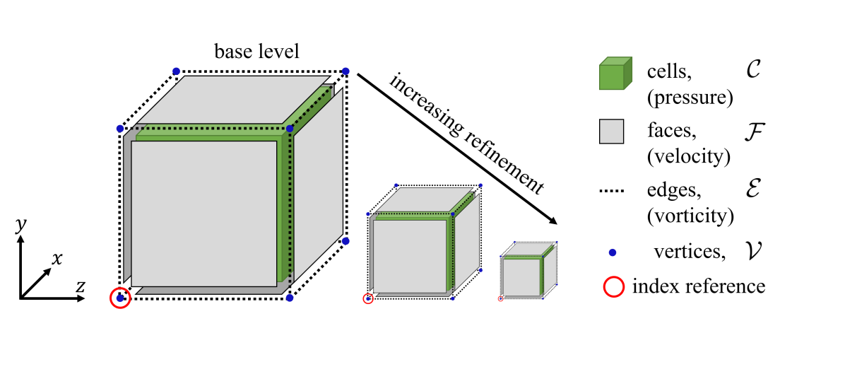
Figure 9: Unit cells of the staggered Cartesian grid at the base and refinement levels of the mesh, showing the locations of relevant flow variables.

The semi-discrete momentum equations, subject to the continuity constraint, are integrated in time using the IF-HERK method (Liska & Colonius, 2016; Yu et al., 2022). This method combines an integrating factor (IF) technique for the viscous term with a half-explicit Runge-Kutta (HERK) technique for the convective term. In the HERK time-stepping scheme (Brasey & Hairer, 1993; Liska & Colonius, 2016; Yu et al., 2022), we subdivide the task of integrating (17) at each time-step into $N_{\rm stage}$ stages. Using a block LU decomposition and the mimetic and commutativity properties of the relevant operators, the subproblem associated with stage $i$ of the HERK scheme is formulated on the composite grid as

$$L_{\mathcal{C}}{\rm p}{}^{i}{}_{\rule{0.0pt}{4.82224pt}\mkern-8.0mu\rm tot}={\rm f}^{i}=D{\rm r}^{i},\quad{\rm u}^{i}=H_{\mathcal{F}}^{i}\left({\rm r}^{i}-G{\rm p}{}^{i}{}_{\rule{0.0pt}{4.82224pt}\mkern-8.0mu\rm tot}\right).$$ (18)

Here, $H$ represents the IF operator and ${\rm f}=D{\rm r}$ approximately represents the divergence of Lamb vector. For brevity, we omit the exact dependencies of ${\rm r}^{i}$ on various flow variables from stages 1 to $i$ of the HERK scheme. We refer to the formulation in section 2.4 of Yu et al. (2022) for these details and for the corresponding Butcher tableau.

While the discrete operators in (17) and (18) are formally defined on the (unbounded) composite grid, they are practically applied to the (finite) subset representing the AMR grid. The operator $R_{\mathcal{Q}}$ restricts variables from the composite grid $\left(\cdot\right)$ to the AMR grid as $\widehat{\left(\cdot\right)}=R_{\mathcal{Q}}\left(\cdot\right)$. In the other direction, the operator $P_{\mathcal{Q}}$ approximates variables on the composite grid using the values on the AMR grid as $\left(\cdot\right)\approx P_{\mathcal{Q}}\widehat{\left(\cdot\right)}$. Using these operators, we can approximate solutions to the subproblems associated with each stage of the HERK formulation in (18) on the AMR grid.

The two steps of each subproblem in (18) involve (i) solving the discrete pressure Poisson equation and (ii) applying the IF to recover the velocity. The solution to the pressure Poisson equation on the AMR grid can be expressed as

$$\widehat{{\rm p}{}^{i}{}_{\rule{0.0pt}{4.82224pt}\mkern-8.0mu\rm tot}}=R_{\mathcal{C}}\mathcal{G}_{\mathcal{C}}*{\rm f}^{i}=R_{\mathcal{C}}L_{\mathcal{C}}^{-1}{\rm f}^{i}\approx R_{\mathcal{C}}L_{\mathcal{C}}^{-1}P_{\mathcal{C}}\widehat{{\rm f}^{i}},$$ (19)

where $\mathcal{G}_{\mathcal{C}}$ is the LGF and $*$ represents the discrete convolution. We efficiently evaluate (19) using a fast multipole method (Liska & Colonius, 2014; Dorschner et al., 2020) that accelerates solutions by incorporating summation techniques based on the fast Fourier transform. This method also key to enabling the linear algorithmic complexity and high parallel efficiency of the flow solver. The application of the IF operator can similarly be expressed as

$${\rm u}^{i}=R_{\mathcal{F}}H_{\mathcal{F}}^{i}\left({\rm r}^{i}-G{\rm p}{}^{i}{}_{\rule{0.0pt}{4.82224pt}\mkern-8.0mu\rm tot}\right)\approx R_{\mathcal{F}}H_{\mathcal{F}}^{i}P_{\mathcal{F}}\left(\widehat{{\rm r}^{i}}-\widehat{G{\rm p}{}^{i}{}_{\rule{0.0pt}{4.82224pt}\mkern-8.0mu\rm tot}}\right),$$ (20)

where $\widehat{G{\rm p}{}^{i}{}_{\rule{0.0pt}{4.82224pt}\mkern-8.0mu\rm tot}}=R_{\mathcal{C}}G{\rm p}{}^{i}{}_{\rule{0.0pt}{4.82224pt}\mkern-8.0mu\rm tot}$. The application of the IF operator represents a convolution with an exponentially decaying kernel and it can also be evaluated using fast LGF techniques (Liska & Colonius, 2016; Yu et al., 2022).

At each time-step, the simulation adapts the extent of the AMR grid and adaptively refines regions within the AMR grid according to the spatial adaptivity and mesh refinement criteria, respectively. The spatial adaptivity criterion sets the boundaries of the AMR grid to capture regions where the source of the pressure Poisson equation exceeds a threshold, $\varepsilon_{\rm adapt}$, relative to its maximum value in the domain. In other words, the AMR grid is adaptively truncated to capture the subset of the unbounded domain satisfying

$$\lvert{\rm f}(\boldsymbol{x},t)\rvert<\varepsilon_{\rm adapt}\lVert{\rm f}\rVert_{\infty}(t).$$ (21)

One caveat is that the IF convolution involves a velocity source that decays slower than vorticity. Correspondingly, its evaluation requires the velocity field in a slightly extended domain based on a cutoff distance that is selected to capture the IF kernel with high accuracy. For the present simulation, the initial rectangular domain is large enough to contain as a subset the domain satisfying the adaptivity criterion (21).

The mesh refinement criteria are formulated in terms of a combined source, ${\rm f}_{k}(t)$, which accounts for the source of the pressure Poisson equation and a correction term at each level $k$. The correction term accounts for the differences between the partial solutions on the coarse and fine grids and it is evaluated using an extended region that can overlap with neighboring levels. We refer to Yu et al. (2022) for the details of its formulation and implementation, which we omit for brevity. Using the combined source, a region is refined or coarsened when

$${\rm f}_{k}(\boldsymbol{x},t)>\alpha^{N_{\rm level}-k}{\rm f}_{\rm max}(t)\;\quad\;{\rm or}\;\quad\;{\rm f}_{k}(\boldsymbol{x},t)<\beta\alpha^{N_{\rm level}-k}{\rm f}_{\rm max}(t),$$ (22)

respectively, where $\alpha\in(0,1)$ and $\beta\in(0,1)$ and we select $\alpha=0.125$ and $\beta=0.875$ for the present simulation. In these criteria, the combined source is evaluated relative to its maximum blockwise root-mean-square (BRMS) value computed over all blocks and previous times, which is expressed as

$${\rm f}_{\rm max}(t)=\max_{\tau<t}{\rm BRMS}\left({\rm f}_{k}(\boldsymbol{x},\tau)\right).$$ (23)

Appendix B Shear-Rotation Correlations and Vortical Flow Structures

The visualizations in figure 3 help identify antiparallel vortex filaments and interactions between vortices, but the comparisons between the vortex boundary ($\Omega_{r}=0.52$) and core ($\Omega_{r}=0.93$) structures provide relatively little information. In figure 10, we visualize the same vortex structures but instead color them using $2\boldsymbol{\dot{\varphi}}\mkern-5.0mu:\mkern-5.0mu\boldsymbol{\dot{\gamma}}/\tilde{W}^{2}$ to probe how conditions conducive to the elliptic instability are structured throughout the vortices in the flow.

As the vortex boundaries merge and expand radially, the shear-rotation correlations are relatively large at the collision plane and the outer boundaries in $z$ and they are relatively small at the inner and outer boundaries in the radial direction. This structuring illustrates how shear-rotation correlations are especially enhanced in regions where the vortex boundaries become thinner, corresponding to the shift from a rigid-rotation-dominated regime to a shearing-dominated regime. During transition, the secondary vortex filaments are initially associated with relatively high and low shear-rotation correlations near their boundaries and cores, respectively. As the turbulence develops, this structuring of $2\boldsymbol{\dot{\varphi}}\mkern-5.0mu:\mkern-5.0mu\boldsymbol{\dot{\gamma}}/\tilde{W}^{2}$ within the vortices remains similar to that of the secondary vortices mediating transition.

This persistent partitioning opens up an interesting possibility of analyzing the action of various mechanisms (e.g., the elliptic instability and the Crow instability) in turbulent flows based on their proximity to vortex cores. For example, the phase space transformations in section 5 can be used to characterize local streamline geometries throughout vortices using the structure of the shear-rotation correlations. Consistent with the transformations depicted in figure 8, our results suggest that local streamlines are more elliptic near vortex boundaries and more circular near vortex cores. This conceptual picture is consistent with the notion that the breakup and displacement of vortex core structures can be associated with the elliptic and Crow instabilities, respectively.

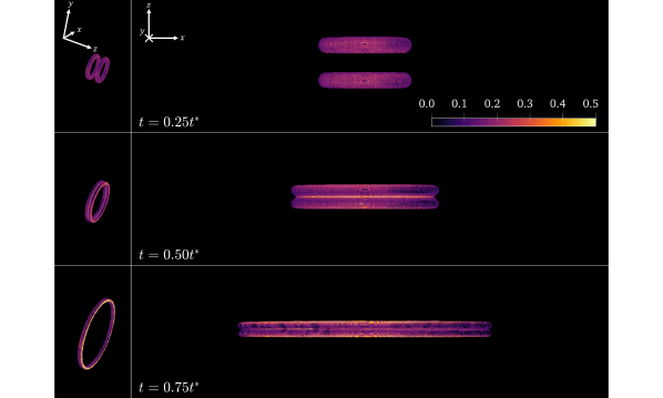
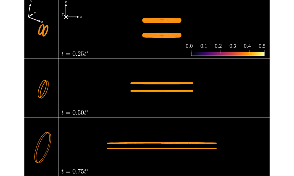
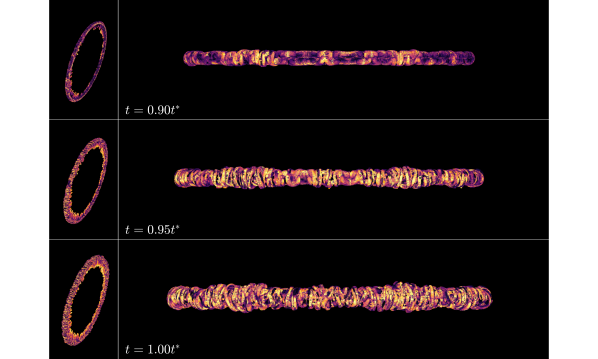
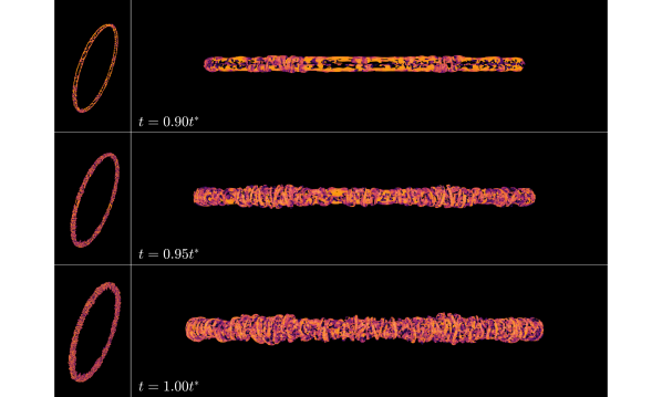
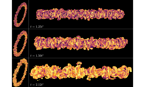
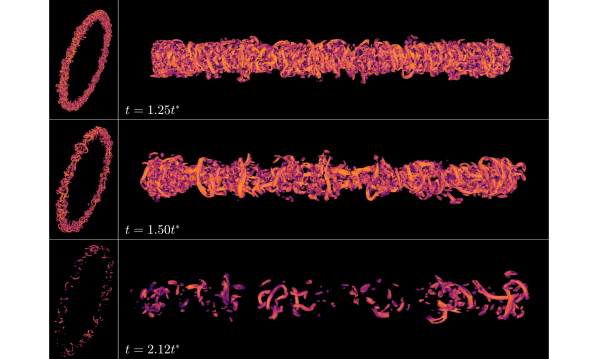
Figure 10: Visualizations of the vortex boundaries ($\Omega_{r}=0.52$, left side) and vortex cores ($\Omega_{r}=0.93$, right side), colored by $2\boldsymbol{\dot{\varphi}}\mkern-5.0mu:\mkern-5.0mu\boldsymbol{\dot{\gamma}}/\tilde{W}^{2}$, for each reference time from table 1. A movie depicting the evolution of the vortex boundaries from the auxiliary viewpoint (leftmost column) is provided as supplementary material.

Appendix C Effect of Shear-Rotation Alignment

Here, we characterize the effect of the alignment between shearing and rigid rotation, as measured by $\theta_{\omega}$, on the phase space transformations associated with rotational local streamline geometries. Figure 11 depicts how the corresponding transformations vary with $\theta_{\omega}$ in the $q_{\rule{0.0pt}{4.82224pt}\mkern-3.0muA}-\,r_{\rule{0.0pt}{4.82224pt}\mkern-4.0muA}$ phase space. When $\theta_{\omega}=90^{\circ}$, shearing and rigid rotation occur in orthogonal planes. In this case, $2\boldsymbol{\dot{\varphi}}\mkern-5.0mu:\mkern-5.0mu\boldsymbol{\dot{\gamma}}=0$, $\zeta=1$, and the region where $\dot{\varphi}^{2}$ dominates $A^{2}$ extends the furthest from the external boundary of the phase space. When $\theta_{\omega}=45^{\circ}$, the regions where $\dot{\varphi}^{2}$ and $\zeta$ are large concentrate more sharply near the external boundary and $2\boldsymbol{\dot{\varphi}}\mkern-5.0mu:\mkern-5.0mu\boldsymbol{\dot{\gamma}}$ grows in the intermediate region between the boundaries of the rotational geometries. The concentration of $\dot{\varphi}^{2}$ and $\zeta$ and the amplification of $2\boldsymbol{\dot{\varphi}}\mkern-5.0mu:\mkern-5.0mu\boldsymbol{\dot{\gamma}}$ are most extreme when $\theta_{\omega}=0^{\circ}$. In this case, the peak contribution of $2\boldsymbol{\dot{\varphi}}\mkern-5.0mu:\mkern-5.0mu\boldsymbol{\dot{\gamma}}$ is $(\sqrt{2}+1)^{-1}$ (Das & Girimaji, 2020b) and, for all $\theta_{\omega}<90^{\circ}$, it occurs when $r_{\rule{0.0pt}{4.82224pt}\mkern-4.0muA}=0$. The location of this maximum approaches $q_{\rule{0.0pt}{4.82224pt}\mkern-3.0muA}\rightarrow\frac{1}{4}$ as $\theta_{\omega}\rightarrow 90^{\circ}$ and $q_{\rule{0.0pt}{4.82224pt}\mkern-3.0muA}\rightarrow\frac{1}{2\sqrt{2}}$ as $\theta_{\omega}\rightarrow 0^{\circ}$. The qualitative features of the distributions vary more significantly from $\theta_{\omega}=90^{\circ}$ to $\theta_{\omega}=45^{\circ}$ than they do from $\theta_{\omega}=45^{\circ}$ to $\theta_{\omega}=0^{\circ}$.

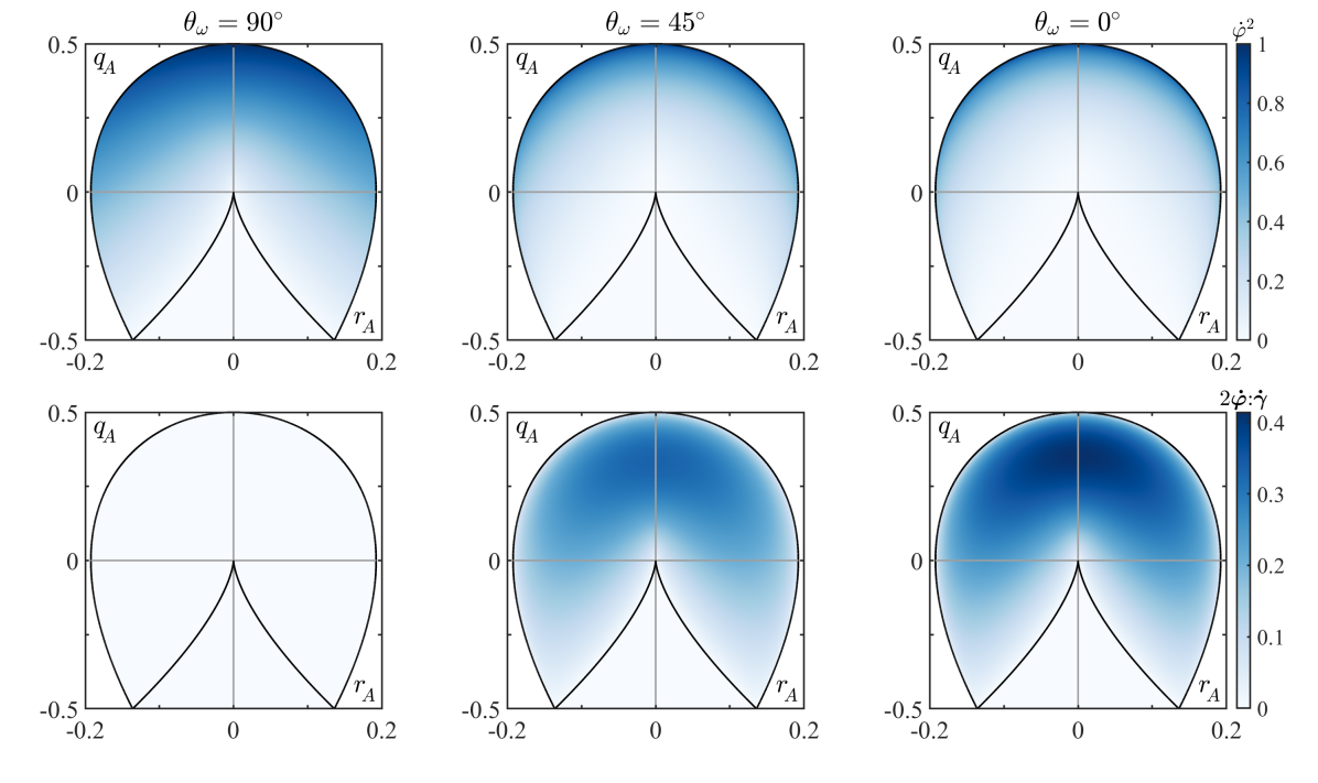
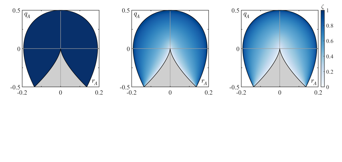
Figure 11: Transformations to $\dot{\varphi}^{2}$, $2\boldsymbol{\dot{\varphi}}\mkern-5.0mu:\mkern-5.0mu\boldsymbol{\dot{\gamma}}$, and $\zeta$ from the $q_{\rule{0.0pt}{4.82224pt}\mkern-3.0muA}-\,r_{\rule{0.0pt}{4.82224pt}\mkern-4.0muA}$ phase space for various alignment angles, $\theta_{\omega}$. The plots are in the same style as those in figure 6.

References

- Archer et al. (2008) Archer, P. J., Thomas, T. G. & Coleman, G. N. 2008 Direct numerical simulation of vortex ring evolution from the laminar to the early turbulent regime. Journal of Fluid Mechanics 598, 201–226.
- Archer et al. (2010) Archer, P. J., Thomas, T. G. & Coleman, G. N. 2010 The instability of a vortex ring impinging on a free surface. Journal of Fluid Mechanics 642, 79–94.
- Arvidsson et al. (2016) Arvidsson, P. M., Kovács, S. J., Töger, J., Borgquist, R., Heiberg, E., Carlsson, M. & Arheden, H. 2016 Vortex ring behavior provides the epigenetic blueprint for the human heart. Scientific Reports 6 (1), 22021.
- Balakrishna et al. (2020) Balakrishna, N., Mathew, J. & Samanta, A. 2020 Inviscid and viscous global stability of vortex rings. Journal of Fluid Mechanics 902, A9.
- Bergdorf et al. (2007) Bergdorf, M., Koumoutsakos, P. & Leonard, A. 2007 Direct numerical simulations of vortex rings at . Journal of Fluid Mechanics 581, 495–505.
- Blanco-Rodríguez & Le Dizès (2016) Blanco-Rodríguez, F. J. & Le Dizès, S. 2016 Elliptic instability of a curved batchelor vortex. Journal of Fluid Mechanics 804, 224–247.
- Blanco-Rodríguez & Le Dizès (2017) Blanco-Rodríguez, F. J. & Le Dizès, S. 2017 Curvature instability of a curved batchelor vortex. Journal of Fluid Mechanics 814, 397–415.
- Blanco-Rodríguez et al. (2015) Blanco-Rodríguez, F. J., Le Dizès, S., Selçuk, C., Delbende, I. & Rossi, M. 2015 Internal structure of vortex rings and helical vortices. Journal of Fluid Mechanics 785, 219–247.
- Brasey & Hairer (1993) Brasey, V. & Hairer, E. 1993 Half-explicit Runge–Kutta methods for differential-algebraic systems of index 2. SIAM Journal on Numerical Analysis 30 (2), 538–552.
- Bush et al. (2003) Bush, J. W. M., Thurber, B. A. & Blanchette, F. 2003 Particle clouds in homogeneous and stratified environments. Journal of Fluid Mechanics 489, 29–54.
- Chakraborty et al. (2005) Chakraborty, P., Balachandar, S. & Adrian, R. J. 2005 On the relationships between local vortex identification schemes. Journal of Fluid Mechanics 535, 189–214.
- Chang & Llewellyn Smith (2021) Chang, C. & Llewellyn Smith, S. G. 2021 Density and surface tension effects on vortex stability. Part 2. Moore–Saffman–Tsai–Widnall instability. Journal of Fluid Mechanics 913, A15.
- Cheng et al. (2016) Cheng, M., Lou, J. & Lim, T. T. 2016 Evolution of an elliptic vortex ring in a viscous fluid. Physics of Fluids 28 (3), 037104.
- Cheng et al. (2018) Cheng, M., Lou, J. & Lim, T. T. 2018 Numerical simulation of head-on collision of two coaxial vortex rings. Fluid Dynamics Research 50 (6), 065513.
- Cheng et al. (2019) Cheng, M., Lou, J. & Lim, T. T. 2019 Collision and reconnection of viscous elliptic vortex rings. Physics of Fluids 31 (6), 067107.
- Chong et al. (1990) Chong, M. S., Perry, A. E. & Cantwell, B. J. 1990 A general classification of three‐dimensional flow fields. Physics of Fluids A: Fluid Dynamics 2 (5), 765–777.
- Chu et al. (1995) Chu, C., Wang, C., Chang, C., Chang, R. & Chang, W. 1995 Head-on collision of two coaxial vortex rings: experiment and computation. Journal of Fluid Mechanics 296, 39–71.
- Crow (1970) Crow, S. C. 1970 Stability theory for a pair of trailing vortices. AIAA Journal 8 (12), 2172–2179.
- Cummins et al. (2018) Cummins, C., Seale, M., Macente, A., Certini, D., Mastropaolo, E., Viola, I. M. & Nakayama, N. 2018 A separated vortex ring underlies the flight of the dandelion. Nature 562 (7727), 414–418.
- Dabiri (2005) Dabiri, J. O. 2005 Flow patterns generated by oblate medusan jellyfish: Field measurements and laboratory analyses. Journal of Experimental Biology 208 (7), 1257–1265.
- Das & Girimaji (2019) Das, R. & Girimaji, S. S. 2019 On the Reynolds number dependence of velocity-gradient structure and dynamics. Journal of Fluid Mechanics 861, 163–179.
- Das & Girimaji (2020a) Das, R. & Girimaji, S. S. 2020a Characterization of velocity-gradient dynamics in incompressible turbulence using local streamline geometry. Journal of Fluid Mechanics 895, A5.
- Das & Girimaji (2020b) Das, R. & Girimaji, S. S. 2020b Revisiting turbulence small-scale behavior using velocity gradient triple decomposition. New Journal of Physics 22 (6), 063015.
- Das & Girimaji (2022) Das, R. & Girimaji, S. S. 2022 The effect of large-scale forcing on small-scale dynamics of incompressible turbulence. Journal of Fluid Mechanics 941, A34.
- Dazin et al. (2006) Dazin, A., Dupont, P. & Stanislas, M. 2006 Experimental characterization of the instability of the vortex rings. Part II: Non-linear phase. Experiments in Fluids 41 (3), 401–413.
- Dong et al. (2019) Dong, X., Gao, Y. & Liu, C. 2019 New normalized Rortex/vortex identification method. Physics of Fluids 31 (1), 011701.
- Dong et al. (2018) Dong, X., Wang, Y., Chen, X., Dong, Y., Zhang, Y. & Liu, C. 2018 Determination of epsilon for Omega vortex identification method. Journal of Hydrodynamics 30 (4), 541–548.
- Dorschner et al. (2020) Dorschner, B., Yu, K., Mengaldo, G. & Colonius, T. 2020 A fast multi-resolution lattice Green’s function method for elliptic difference equations. Journal of Computational Physics 407, 109270.
- Epps (2017) Epps, B. P. 2017 Review of vortex identification methods. In 55th AIAA Aerospace Sciences Meeting, p. 2017–0989. Grapevine, Texas.
- Fukumoto & Hattori (2005) Fukumoto, Y. & Hattori, Y. 2005 Curvature instability of a vortex ring. Journal of Fluid Mechanics 526, 77–115.
- Gao & Liu (2018) Gao, Y. & Liu, C. 2018 Rortex and comparison with eigenvalue-based vortex identification criteria. Physics of Fluids 30 (8), 085107.
- Gao & Liu (2019) Gao, Y. & Liu, C. 2019 Rortex based velocity gradient tensor decomposition. Physics of Fluids 31 (1), 011704.
- Gao et al. (2019) Gao, Y., Yu, Y., Liu, J. & Liu, C. 2019 Explicit expressions for Rortex tensor and velocity gradient tensor decomposition. Physics of Fluids 31 (8), 081704.
- Gharib et al. (1998) Gharib, M., Rambod, E. & Shariff, K. 1998 A universal time scale for vortex ring formation. Journal of Fluid Mechanics 360, 121–140.
- Girimaji & Speziale (1995) Girimaji, S. S. & Speziale, C. G. 1995 A modified restricted euler equation for turbulent flows with mean velocity gradients. Physics of Fluids 7 (6), 1438–1446.
- Günther & Theisel (2018) Günther, T. & Theisel, H. 2018 The state of the art in vortex extraction. Computer Graphics Forum 37 (6), 149–173.
- Haller (2021) Haller, G. 2021 Can vortex criteria be objectivized? Journal of Fluid Mechanics 908, A25.
- Hattori et al. (2019) Hattori, Y., Blanco-Rodríguez, F. J. & Le Dizès, S. 2019 Numerical stability analysis of a vortex ring with swirl. Journal of Fluid Mechanics 878, 5–36.
- Hoffman (2021) Hoffman, J. 2021 Energy stability analysis of turbulent incompressible flow based on the triple decomposition of the velocity gradient tensor. Physics of Fluids 33 (8), 081707.
- Hunt et al. (1988) Hunt, J. C. R., Wray, A. A. & Moin, P. 1988 Eddies, streams, and convergence zones in turbulent flows. In Proceedings of the 1988 Summer Program, pp. 193–208. Center for Turbulence Research, Stanford, CA.
- Jeong & Hussain (1995) Jeong, J. & Hussain, F. 1995 On the identification of a vortex. Journal of Fluid Mechanics 285, 69–94.
- Johnson (2005) Johnson, W. 2005 Model for vortex ring state influence on rotorcraft flight dynamics. Tech. Rep. NASA/TP-2005-213477. National Aeronautics and Space Administration.
- Kerswell (2002) Kerswell, R. R. 2002 Elliptical instability. Annual Review of Fluid Mechanics 34 (1), 83–113.
- Keylock (2018) Keylock, C. J. 2018 The Schur decomposition of the velocity gradient tensor for turbulent flows. Journal of Fluid Mechanics 848, 876–905.
- Kida et al. (1991) Kida, S., Takaoka, M. & Hussain, F. 1991 Collision of two vortex rings. Journal of Fluid Mechanics 230, 583–646.
- Kolář (2004) Kolář, V. 2004 2D velocity-field analysis using triple decomposition of motion. In Proceedings of the 15th Australasian Fluid Mechanics Conference, p. AFMC00017. The University of Sydney.
- Kolář (2007) Kolář, V. 2007 Vortex identification: New requirements and limitations. International Journal of Heat and Fluid Flow 28 (4), 638–652.
- Kolář & Šístek (2020) Kolář, V. & Šístek, J. 2020 Consequences of the close relation between rortex and swirling strength. Physics of Fluids 32 (9), 091702.
- Kolář & Šístek (2022) Kolář, V. & Šístek, J. 2022 Disappearing vortex problem in vortex identification: Non-existence for selected criteria. Physics of Fluids 34 (7), 071704.
- Krueger & Gharib (2003) Krueger, P. S. & Gharib, M. 2003 The significance of vortex ring formation to the impulse and thrust of a starting jet. Physics of Fluids 15 (5), 1271–1281.
- Kyle et al. (2020) Kyle, R., Lee, Y. C. & Früh, W. 2020 Propeller and vortex ring state for floating offshore wind turbines during surge. Renewable Energy 155, 645–657.
- Leweke et al. (2016) Leweke, T., Le Dizès, S. & Williamson, C. H. K. 2016 Dynamics and instabilities of vortex pairs. Annual Review of Fluid Mechanics 48 (1), 507–541.
- Lim & Nickels (1992) Lim, T. & Nickels, T. 1992 Instability and reconnection in the head-on collision of two vortex rings. Nature 357, 225–227.
- Limbourg & Nedić (2021) Limbourg, R. & Nedić, J. 2021 Formation of an orifice-generated vortex ring. Journal of Fluid Mechanics 913, A29.
- Liska (2016) Liska, S. 2016 Fast lattice Green’s function methods for viscous incompressible flows on unbounded domains. PhD Thesis, California Institute of Technology, Pasadena, CA.
- Liska & Colonius (2014) Liska, S. & Colonius, T. 2014 A parallel fast multipole method for elliptic difference equations. Journal of Computational Physics 278, 76–91.
- Liska & Colonius (2016) Liska, S. & Colonius, T. 2016 A fast lattice Green’s function method for solving viscous incompressible flows on unbounded domains. Journal of Computational Physics 316, 360–384.
- Liu et al. (2019a) Liu, C., Gao, Y., Dong, X., Wang, Y., Liu, J., Zhang, Y., Cai, X. & Gui, N. 2019a Third generation of vortex identification methods: Omega and Liutex/Rortex based systems. Journal of Hydrodynamics 31 (2), 205–223.
- Liu et al. (2018) Liu, C., Gao, Y., Tian, S. & Dong, X. 2018 Rortex–a new vortex vector definition and vorticity tensor and vector decompositions. Physics of Fluids 30 (3), 035103.
- Liu et al. (2016) Liu, C., Wang, Y., Yang, Y. & Duan, Z. 2016 New omega vortex identification method. Science China Physics, Mechanics & Astronomy 59 (8), 684711.
- Liu et al. (2019b) Liu, J., Gao, Y. & Liu, C. 2019b An objective version of the Rortex vector for vortex identification. Physics of Fluids 31 (6), 065112.
- Liu et al. (2019c) Liu, J., Gao, Y., Wang, Y. & Liu, C. 2019c Objective Omega vortex identification method. Journal of Hydrodynamics 31 (3), 455–463.
- Liu & Liu (2019) Liu, J. & Liu, C. 2019 Modified normalized Rortex/vortex identification method. Physics of Fluids 31 (6), 061704.
- Lopez & Bulbeck (1993) Lopez, J. M. & Bulbeck, C. J. 1993 Behavior of streamwise rib vortices in a three‐dimensional mixing layer. Physics of Fluids A: Fluid Dynamics 5 (7), 1694–1702.
- McKeown et al. (2018) McKeown, R., Ostilla-Mónico, R., Pumir, A., Brenner, M. P. & Rubinstein, S. M. 2018 Cascade leading to the emergence of small structures in vortex ring collisions. Physical Review Fluids 3 (12), 124702.
- McKeown et al. (2020) McKeown, R., Ostilla-Mónico, R., Pumir, A., Brenner, M. P. & Rubinstein, S. M. 2020 Turbulence generation through an iterative cascade of the elliptical instability. Science Advances 6 (9), eaaz2717.
- Mishra et al. (2021) Mishra, A., Pumir, A. & Ostilla-Mónico, R. 2021 Instability and disintegration of vortex rings during head-on collisions and wall interactions. Physical Review Fluids 6 (10), 104702.
- Mohseni et al. (2001) Mohseni, K., Ran, H. & Colonius, T. 2001 Numerical experiments on vortex ring formation. Journal of Fluid Mechanics 430, 267–282.
- Moore & Saffman (1975) Moore, D. W. & Saffman, P. G. 1975 The instability of a straight vortex filament in a strain field. Proceedings of the Royal Society of London. A. Mathematical and Physical Sciences 346 (1646), 413–425.
- Nagata et al. (2020) Nagata, R., Watanabe, T., Nagata, K. & da Silva, C. B. 2020 Triple decomposition of velocity gradient tensor in homogeneous isotropic turbulence. Computers & Fluids 198, 104389.
- Nguyen et al. (2021) Nguyen, V. L., Phan, T. T., Duong, V. D. & Le, N. T. P. 2021 Turbulent energy cascade associated with viscous reconnection of two vortex rings. Physics of Fluids 33 (8), 085117.
- O’Farrell & Dabiri (2014) O’Farrell, C. & Dabiri, J. O. 2014 Pinch-off of non-axisymmetric vortex rings. Journal of Fluid Mechanics 740, 61–96.
- Oshima (1978) Oshima, Y. 1978 Head-on collision of two vortex rings. Journal of the Physical Society of Japan 44 (1), 328–331.
- Ostilla-Mónico et al. (2021) Ostilla-Mónico, R., McKeown, R., Brenner, M. P., Rubinstein, S. M. & Pumir, A. 2021 Cascades and reconnection in interacting vortex filaments. Physical Review Fluids 6 (7), 074701.
- Perry & Chong (1987) Perry, A. E. & Chong, M. S. 1987 A description of eddying motions and flow patterns using critical-point concepts. Annual Review of Fluid Mechanics 19 (1), 125–155.
- Perry & Fairlie (1975) Perry, A. E. & Fairlie, B. D. 1975 Critical points in flow patterns. Advances in Geophysics 18, 299–315.
- Ruggaber (2000) Ruggaber, G. J. 2000 Dynamics of particle clouds related to open-water sediment disposal. PhD Thesis, Massachusetts Institute of Technology, Cambridge, MA.
- Saffman (1993) Saffman, P. G. 1993 Vortex Dynamics. Cambridge University Press.
- Serrin (1959) Serrin, J. 1959 Mathematical Principles of Classical Fluid Mechanics, Handbuch der Physik, vol. 8/1, pp. 125–263. Berlin, Heidelberg: Springer.
- Shariff & Leonard (1992) Shariff, K. & Leonard, A. 1992 Vortex rings. Annual Review of Fluid Mechanics 24, 235–279.
- Shariff et al. (1994) Shariff, K., Verzicco, R. & Orlandi, P. 1994 A numerical study of three-dimensional vortex ring instabilities: Viscous corrections and early nonlinear stage. Journal of Fluid Mechanics 279, 351–375.
- Sharma et al. (2021) Sharma, B., Das, R. & Girimaji, S. S. 2021 Local vortex line topology and geometry in turbulence. Journal of Fluid Mechanics 924, A13.
- Smith & Wei (1994) Smith, G. B. & Wei, T. 1994 Small-scale structure in colliding off-axis vortex rings. Journal of Fluid Mechanics 259, 281–290.
- Taddeucci et al. (2015) Taddeucci, J., Alatorre-Ibarguengoitia, M. A., Palladino, D. M., Scarlato, P. & Camaldo, C. 2015 High-speed imaging of Strombolian eruptions: Gas-pyroclast dynamics in initial volcanic jets. Geophysical Research Letters 42 (15), 6253–6260.
- Tian et al. (2018) Tian, S., Gao, Y., Dong, X. & Liu, C. 2018 Definitions of vortex vector and vortex. Journal of Fluid Mechanics 849, 312–339.
- Tom et al. (2021) Tom, J., Carbone, M. & Bragg, A. D. 2021 Exploring the turbulent velocity gradients at different scales from the perspective of the strain-rate eigenframe. Journal of Fluid Mechanics 910, A24.
- Towns et al. (2014) Towns, J., Cockerill, T., Dahan, M., Foster, I., Gaither, K., Grimshaw, A., Hazlewood, V., Lathrop, S., Lifka, D., Peterson, G. D., Roskies, R., Scott, J. R. & N., Wilkins-Diehr 2014 XSEDE: Accelerating scientific discovery. Computing in Science and Engineering 16 (5), 62–74.
- Tsai & Widnall (1976) Tsai, C. & Widnall, S. E. 1976 The stability of short waves on a straight vortex filament in a weak externally imposed strain field. Journal of Fluid Mechanics 73 (4), 721–733.
- Walker et al. (1987) Walker, J. D. A., Smith, C. R., Cerra, A. W. & Doligalski, T. L. 1987 The impact of a vortex ring on a wall. Journal of Fluid Mechanics 181, 99–140.
- Wang et al. (2018) Wang, Y., Gao, Y. & Liu, C. 2018 Letter: Galilean invariance of Rortex. Physics of Fluids 30 (11), 111701.
- Weigand & Gharib (1994) Weigand, A. & Gharib, M. 1994 On the decay of a turbulent vortex ring. Physics of Fluids 6 (12), 3806–3808.
- Widnall et al. (1974) Widnall, S. E., Bliss, D. B. & Tsai, C. 1974 The instability of short waves on a vortex ring. Journal of Fluid Mechanics 66 (1), 35–47.
- Widnall & Tsai (1977) Widnall, S. E. & Tsai, C. 1977 The instability of the thin vortex ring of constant vorticity. Philosophical Transactions of the Royal Society of London. Series A, Mathematical and Physical Sciences 287 (1344), 273–305.
- Wu et al. (2015) Wu, J., Ma, H. & Zhou, M. 2015 Vortical Flows. Berlin, Heidelberg: Springer.
- Wu et al. (2020) Wu, Y., Zhang, W., Wang, Y., Zou, Z. & Chen, J. 2020 Energy dissipation analysis based on velocity gradient tensor decomposition. Physics of Fluids 32 (3), 035114.
- Yao & Hussain (2020a) Yao, J. & Hussain, F. 2020a On singularity formation via viscous vortex reconnection. Journal of Fluid Mechanics 888, R2.
- Yao & Hussain (2020b) Yao, J. & Hussain, F. 2020b A physical model of turbulence cascade via vortex reconnection sequence and avalanche. Journal of Fluid Mechanics 883, A51.
- Yao & Hussain (2020c) Yao, J. & Hussain, F. 2020c Separation scaling for viscous vortex reconnection. Journal of Fluid Mechanics 900, R4.
- Yao et al. (2021) Yao, J., Yang, Y. & Hussain, F. 2021 Dynamics of a trefoil knotted vortex. Journal of Fluid Mechanics 923, A19.
- Yu (2021) Yu, K. 2021 Multi-resolution lattice Green’s function method for high Reynolds number external flows. PhD Thesis, California Institute of Technology, Pasadena, CA.
- Yu et al. (2022) Yu, K., Dorschner, B. & Colonius, T. 2022 Multi-resolution lattice Green’s function method for incompressible flows. Journal of Computational Physics 459, 110845.
- Zawadzki & Aref (1991) Zawadzki, I. & Aref, H. 1991 Mixing during vortex ring collision. Physics of Fluids A: Fluid Dynamics 3 (5), 1405–1410.
- Zhao et al. (2021) Zhao, X., Yu, Z., Chapelier, J. & Scalo, C. 2021 Direct numerical and large-eddy simulation of trefoil knotted vortices. Journal of Fluid Mechanics 910, A31.