Quantum-embeddable stochastic matrices

Abstract

The classical embeddability problem asks whether a given stochastic matrix $T$, describing transition probabilities of a $d$-level system, can arise from the underlying homogeneous continuous-time Markov process. Here, we investigate the quantum version of this problem, asking of the existence of a Markovian quantum channel generating state transitions described by a given $T$. More precisely, we aim at characterising the set of quantum-embeddable stochastic matrices that arise from memoryless continuous-time quantum evolution. To this end, we derive both upper and lower bounds on that set, providing new families of stochastic matrices that are quantum-embeddable but not classically-embeddable, as well as families of stochastic matrices that are not quantum-embeddable. As a result, we demonstrate that a larger set of transition matrices can be explained by memoryless models if the dynamics is allowed to be quantum, but we also identify a non-zero measure set of random processes that cannot be explained by either classical or quantum memoryless dynamics. Finally, we fully characterise extreme stochastic matrices (with entries given only by zeros and ones) that are quantum-embeddable.

1 Introduction

In 1937, a Finnish mathematician, Gustav Elfving, asked a fundamental question concerning the nature of randomness [1]. Namely, he wondered which of the observed random transitions between discrete states of a given system can be explained by the underlying continuous memoryless process. More precisely, consider a system with $d$ distinguishable states and initially prepared in some state $j$, which then evolves for a time $t_{f}$, and after that the system is measured and found in some state $i$. Repeating this experiment many times and recording the frequency of observed output states for all input states, one recovers a transition matrix $T$ with matrix elements $T_{ij}$ describing the probabilities of state transitions from $j$ to $i$. Elfving then asked, whether the random process observed at time $t_{f}$ and described by $T$ can arise from a homogeneous continuous-time Markov process, i.e., a process acting continuously and identically at all times $t\in[0,t_{f}]$, and such that the evolution of the system at each infinitesimal moment in time depends only on the current state of the system (and not on its history). Formally, this corresponds to the following embedding problem [2]: given a transition matrix $T$, one wants to know whether there exists a family of transition matrices $e^{Lt}$ continuously connecting the identity at $t=0$ with $T=e^{Lt_{f}}$ at $t=t_{f}$. Here, $L$ is a time-independent Markov generator (also known as the rate matrix) that is a $d\times d$ matrix with non-negative off-diagonal entries and columns summing to zero [2].

Despite decades of efforts, complete solutions to the classical embeddability problem described above have only been found for $2\times 2$ [3], $3\times 3$ [4, 5, 6], and very recently also for $4\times 4$ matrices [7]. Nevertheless, the subset of embeddable matrices of general size $d$ can be bounded within the set of all $d\times d$ stochastic matrices, because various necessary conditions for embeddability were found, among them the following one [8]:

$$\prod_{i=1}^{d}T_{ii}\geq\mathrm{det~{}}T\geq 0.$$ (1)

Thus, every continuous-time random process that results in a transition matrix $T$ failing to satisfy the above conditions must necessarily use memory effects. In other words, observing such a random process $T$ only at a discrete moment in time, we can infer that the underlying dynamics cannot be explained with a memoryless model.

In this paper we ask: how the non-existence of a memoryless model explaining a given $T$ is affected if we drop the implicit assumption that the underlying continuous dynamical process is classical and instead allow for a quantum evolution? This means that instead of occupying one of the well-defined $d$ states, the investigated system can be in any coherent superposition of these $d$ states, and the general evolution consists of both classical stochastic jumps and quantum coherent transitions. For the simplest example that we illustrate in Fig. 1, consider a spin-1/2 particle that is initially prepared in one of the two perfectly distinguishable states, either a spin-up state $|{\uparrow}\rangle$ or a spin-down state $|{\downarrow}\rangle$. As in the classical scenario, it is then left to evolve for a time $t_{f}$, after which the orientation of its spin is measured, the procedure is repeated and the outcome frequencies yield the transition matrix $T$. The crucial difference is that the evolution between time $0$ and $t_{f}$ is quantum, and we want to ask whether a given $T$ can arise from a memoryless quantum dynamics.

This problem of quantum-embeddability of stochastic matrices was recently introduced in Ref. [9], where the authors focused on a more general concept of memoryless quantum dynamics that is time-inhomogeneous, i.e., the generator of the evolution may change in time. Here, in the spirit of the original Elfving problem, we want to characterise the set of transition matrices that can arise from the underlying homogeneous continuous-time quantum Markov process. Our main results consist of lower and upper bounds on the set of quantum-embeddable stochastic matrices, i.e., we identify both a new family of stochastic matrices that are quantum-embeddable (but not classically-embeddable) and a family of stochastic matrices that are not quantum-embeddable (neither classically-embeddable). As a result, we find a whole class of random processes that cannot arise from either a classical or quantum memoryless dynamics. Therefore, observing such a process only at a discrete moment in time, we can infer that the underlying dynamics is non-Markovian.

The paper is structured as follows. First, in Sec. 2, we provide the mathematical background for our studies and formally state the investigated problem. Then, in Sec. 3, we present and discuss our main results concerning families of transition matrices that are not quantum-embeddable, and those that are. Section 4 contains step-by-step derivations of our results together with intermediate results that may be of independent interest. Finally, Sec. 5 contains conclusions and an outlook for future work.

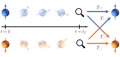
Figure 1: Transition matrices arising from memoryless quantum dynamics. A two-level quantum system prepared initially in one of two perfectly distinguishable states, $|{\uparrow}\rangle$ or $|{\downarrow}\rangle$, undergoes an unknown evolution for time $t_{f}$ after which it is measured in the $\{|{\uparrow}\rangle,|{\downarrow}\rangle\}$ basis. The conditional outcome probabilities, i.e., probabilities $T_{ij}$ of observing $|{i}\rangle$ given that the system started in $|{j}\rangle$ for $i,j\in\{\uparrow,\downarrow\}$, form a transition matrix $T$. One can then ask which observed $T$ can be explained by the underlying time-homogeneous memoryless quantum dynamics. The central problem we investigate in this paper is the generalisation of this question to $d$-dimensional quantum systems.

2 Setting the scene

A state of a $d$-dimensional quantum system is described by a $d\times d$ density matrix $\rho$ that is positive and has unit trace. A general open quantum evolution of such a system is given by a quantum channel ${\mathcal{E}}$, which is a linear map between $d\times d$ matrices that is completely positive and trace-preserving. A channel ${\mathcal{E}}$ is called time-independent embeddable (Markovian) if and only if it is in the closure of the maps of the following form [10]:

$${\mathcal{E}}_{t}=e^{{\mathcal{L}}t},$$ (2)

where $t\in\mathbb{R}_{+}$ denotes a finite time and ${\mathcal{L}}$ is the Lindblad generator satisfying [11, 12]

$${\mathcal{L}}(\cdot)=i[\cdot,H]+\Phi(\cdot)-\frac{1}{2}\{\Phi^{*}(\mathbbm{1}),\cdot\}.$$ (3)

Above, $H$ is Hermitian and physically corresponds to the Hamiltonian of the system that induces the closed unitary dynamics, $\Phi$ is a completely positive (but not necessarily trace-preserving) map that physically describes dissipative open dynamics due to interactions with the environment, $\{\cdot,\cdot\}$ is the anticommutator and $\Phi^{*}$ denotes the dual of $\Phi$, i.e.,

$$\forall{A,B}:~{}~{}\mathrm{Tr}\left(A\Phi(B)\right)=\mathrm{Tr}\left(\Phi^{*}(A)B\right).$$ (4)

To be physically meaningful, ${\mathcal{L}}$ is assumed to have a finite operator norm. Thus, the assumption of closure is necessary in order to include in the set of Markovian channels the non-invertible channels that can be generated by Markovian dynamics with arbitrary precision.

A classical action $T$ of a quantum channel ${\mathcal{E}}$ is defined by a stochastic matrix describing transitions induced by ${\mathcal{E}}$ in a given basis $\{|{i}\rangle\}_{i=1}^{d}$:

$$T_{ij}:=\left\langle i\vphantom{{\mathcal{E}}(\left|j\right\rangle\!\!\left\langle j\right|)i}\right|{\mathcal{E}}(\left|j\right\rangle\!\!\left\langle j\right|)\left|i\vphantom{i{\mathcal{E}}(\left|j\right\rangle\!\!\left\langle j\right|)}\right\rangle.$$ (5)

The set of all $d\times d$ stochastic matrices (i.e., matrices with non-negative entries and columns summing to identity) will be denoted by ${\mathcal{T}}_{d}$. Now, the central notion investigated in this paper is the following time-homogeneous version of quantum-embeddability [9].

Definition 1 (Quantum-embeddable stochastic matrix).

A stochastic matrix $T$ is quantum-embeddable if it is a classical action of some Markovian quantum channel, i.e., if, for any $\delta>0$, there exist a Lindbladian ${\mathcal{L}}$ and a finite time $t_{f}$ such that

$$\max_{i,j}\big{|}T_{ij}-\left\langle i\vphantom{e^{{\mathcal{L}}t_{f}}(\left|j\right\rangle\!\!\left\langle j\right|)i}\right|e^{{\mathcal{L}}t_{f}}(\left|j\right\rangle\!\!\left\langle j\right|)\left|i\vphantom{ie^{{\mathcal{L}}t_{f}}(\left|j\right\rangle\!\!\left\langle j\right|)}\right\rangle\big{|}\leq\delta.$$ (6)

The above definition generalises to the quantum setting the set of classical limit-embeddable stochastic matrices introduced in Ref. [13]. We will denote the set of $d\times d$ quantum-embeddable stochastic matrices by ${\mathcal{Q}}_{d}$ and its complement within the set of $d\times d$ stochastic matrices by ${\mathcal{Q}}_{d}^{c}$. Similarly, the set of classically-embeddable stochastic matrices described in the introduction and its complement will be denoted by ${\mathcal{C}}_{d}$ and ${\mathcal{C}}_{d}^{c}$. Note that both sets ${\mathcal{C}}_{d}$ and ${\mathcal{Q}}_{d}$ are, by definition, closed. Moreover, it is clear that ${\mathcal{C}}_{d}\subset{\mathcal{Q}}_{d}$, since classical processes form a particular subset of quantum processes. This can be shown explicitly by noting that a classically-embeddable $T=e^{Lt_{f}}$ is a classical action of a Markovian quantum channel $e^{{\mathcal{L}}t_{f}}$ with a Lindblad generator defined through Eq. (3) with $H=0$ and

$$\Phi(\cdot)=\sum_{i,j=1}^{d}|L_{ij}|\left|i\right\rangle\!\!\left\langle j\right|(\cdot)\left|j\right\rangle\!\!\left\langle i\right|.$$ (7)

On the other extreme, we can choose $\Phi=0$ and by varying $H$ generate all unitary channels. Thus, ${\mathcal{U}}_{d}\subset{\mathcal{Q}}_{d}$, with ${\mathcal{U}}_{d}$ denoting the set of $d\times d$ unistochastic matrices [14], i.e., matrices $T$ such that $T_{ij}=|U_{ij}|^{2}$ for some unitary matrix $U$. Since there exist matrices in ${\mathcal{U}}_{d}$ but not in ${\mathcal{C}}_{d}$ (e.g., a non-trivial permutation matrix), and there exists matrices in ${\mathcal{C}}_{d}$ and not in ${\mathcal{U}}_{d}$ (e.g., a matrix $T$ with $T_{ij}=\delta_{ik}$ for any fixed $k$), ${\mathcal{Q}}_{d}$ is a strict superset of both ${\mathcal{U}}_{d}$ and ${\mathcal{C}}_{d}$. This lower bounds the set ${\mathcal{Q}}_{d}$ within the set ${\mathcal{T}}_{d}$, and the aim of this paper is to improve this bound, as well as to upper bound ${\mathcal{Q}}_{d}$, i.e., to identify which stochastic matrices are not quantum-embeddable.

3 Results and discussion

Our first result identifies a subset of $2\times 2$ matrices that are not quantum-embeddable.

Theorem 1.

Consider a $2\times 2$ stochastic matrix $T$,

$$T=\begin{pmatrix}a&1-b\\ 1-a&b\end{pmatrix}.$$ (8)

If $a\leq 10^{-6}$ and $f(a)\left(2-f(a)\right)<b<1-g(a)$, then $T\notin{\mathcal{Q}}_{2}$. Here,

$$f(a)= ~{}2\sqrt{2}a^{0.25}+\sqrt{a(2-a)}+a^{0.9}$$ (9a)

$$~{}+\frac{0.01(4\sqrt{a}+a^{0.45})}{1-(8\sqrt{a}+a^{0.45})}+2\sqrt{8\sqrt{a}+a^{0.45}},$$

$$g(a)= ~{}(2-a)(2a+a^{0.1}),$$ (9b)

so that both these functions vanish when $a\to 0$. The same result holds if we swap $a$ for $b$.

The proof of the above theorem can be found in Sec. 4.2, whereas in Sec. 4.1 we present its simplified version that only works for a special case of $a=0$ (or $b=0$ after swapping $a$ for $b$). Here, based on numerical investigations, we note that the bounds on $a$ and $b$ from Theorem 1 are quite loose and most probably can be significantly improved. More precisely, numerically optimising over all Lindblad evolutions of a qubit system (see Appendix A for details), we observe that the numerical bounds on $a$ and $b$ differ by more than four orders of magnitudes from the analytic bounds stated in Theorem 1. We illustrate this in Fig. 2, where in panel (a) the set ${\mathcal{T}}_{2}$ is presented, together with its subsets ${\mathcal{C}}_{2}$ (characterised analytically in Ref. [3]) and ${\mathcal{Q}}_{2}$ (characterised numerically here); whereas in panel (b) we compare the numerical and analytic bounds.

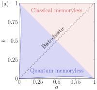
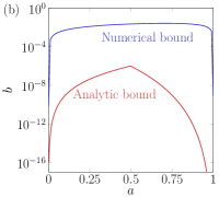
Figure 2: Memoryless dynamics of a two-level system. Every $2\times 2$ stochastic matrix representing the evolution of a two-level system (see Eq. (8)) can be represented as a point inside a square $(a,b)\in[0,1]\times[0,1]$. (a) The upper-right red region contains classically-embeddable matrices, whereas the bottom-left blue region contains those quantum-embeddable matrices that are not classically-embeddable. For transitions described by matrices belonging to the white region (left or below the blue bounding curves obtained through numerical optimisations) there are no memoryless models (classical or quantum) explaining them. (b) Comparison of the analytical and numerical bound for the set ${\mathcal{Q}}_{2}$: above the top blue curve all matrices are quantum-embeddable, whereas below the bottom red curve no matrices are quantum-embeddable. The real boundary between ${\mathcal{Q}}_{2}$ and ${\mathcal{Q}}_{2}^{c}$ lies somewhere between the two curves.

Theorem 1 shows that ${\mathcal{Q}}_{2}^{c}$ occupies a non-zero volume within the set ${\mathcal{T}}_{2}$ and thus upper bounds ${\mathcal{Q}}_{2}$ (note that this is contrary to the case of time-dependent generators, where the entire ${\mathcal{T}}_{2}$ can be generated by time-inhomogeneous quantum Markovian dynamics [9]). Our second result provides such an upper bound for higher dimensional systems. Namely, the following theorem identifies a family of matrices belonging to ${\mathcal{Q}}_{d}^{c}$ and so, since ${\mathcal{Q}}_{d}^{c}$ is non-empty and open, it shows that ${\mathcal{Q}}_{d}^{c}$ has a non-zero measure, which in turn yields an upper bound on ${\mathcal{Q}}_{d}$.

Theorem 2.

Consider a $d\times d$ stochastic matrix $T$. Let ${\mathcal{I}}_{0}\subset\{1,\cdots,d\}$ be a subset of indices such that $T$ invariantly permutes ${\mathcal{I}}_{0}$. Also, let ${\mathcal{I}}_{1}\subset{\mathcal{I}}_{0}^{c}$ denote a subset of the complementary set of ${\mathcal{I}}_{0}$, where for any $i_{1}\in{\mathcal{I}}_{1}$ it holds that $T_{i_{0}i_{1}}=1$ for some fixed $i_{0}\in{\mathcal{I}}_{0}$. Then, $T\in{\mathcal{Q}}_{d}^{c}$ if there exists an index $i$ such that

$$\sum_{i_{1}\in{\mathcal{I}}_{1}}T_{i_{1}i}=1.$$ (10)

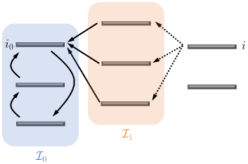
Figure 3: Visualisation of Theorem 2. An example of a transition matrix for a $d=8$ level system that is not quantum-embeddable according to Theorem 2. Solid arrows denote deterministic transitions (with probability 1), dotted arrows denote probabilistic transitions, and a lack of arrows from a given level means that arbitrary transitions from that level are allowed.

The proof of the above theorem can be found in Sec. 4.3, whereas in Fig. 3 we illustrate the sets, states and transitions appearing in the statement of the theorem to better visualise its content. Here, we will unpack Theorem 2 by examining the lowest possible dimensions of $d=3$ and $d=4$. For $d=3$, the structure imposed by the theorem requires ${\mathcal{I}}_{0}$ to be one-dimensional. Thus, $T$ acts trivially on ${\mathcal{I}}_{0}=\{i_{0}\}$, i.e., $T_{i_{0}i_{0}}=1$. Moreover, ${\mathcal{I}}_{1}$ also needs to be one-dimensional. For different choices of $i_{0}$ and $i_{1}$, we then obtain that the following six extreme stochastic matrices are not quantum-embeddable:

$$\left\{\begin{pmatrix}1&1&0\\ 0&0&1\\ 0&0&0\end{pmatrix},\begin{pmatrix}1&0&1\\ 0&0&0\\ 0&1&0\end{pmatrix},\begin{pmatrix}0&0&1\\ 1&1&0\\ 0&0&0\end{pmatrix},\right.$$ (11)

$$\left.~{}~{}\begin{pmatrix}0&0&0\\ 0&1&1\\ 1&0&0\end{pmatrix},\begin{pmatrix}0&1&0\\ 0&0&0\\ 1&0&1\end{pmatrix},\begin{pmatrix}0&0&0\\ 1&0&0\\ 0&1&1\end{pmatrix}\right\}.$$

Therefore, no $3\times 3$ transition matrices in the vicinity of the above matrices can result from time-homogeneous Markovian quantum dynamics. Taking $d=4$ brings more freedom to construct not only a discrete set of extreme stochastic matrices belonging to ${\mathcal{Q}}_{4}^{c}$, but also continuous families of stochastic matrices in ${\mathcal{Q}}_{4}^{c}$ located at the boundaries of ${\mathcal{T}}_{4}$. For example, let us fix ${\mathcal{I}}_{0}=\{1\}$ and ${\mathcal{I}}_{1}=\{m,n\}$ for different choices of $m,n\in\{2,3,4\}$. Then, Theorem 2 yields the following three families of matrices in ${\mathcal{Q}}_{4}^{c}$:

$$\left\{\!\begin{pmatrix}1&1&1&0\\ 0&0&0&p\\ 0&0&0&q\\ 0&0&0&0\end{pmatrix},\!\begin{pmatrix}1&1&0&1\\ 0&0&p&0\\ 0&0&0&0\\ 0&0&q&0\end{pmatrix},\!\begin{pmatrix}1&0&1&1\\ 0&0&0&0\\ 0&p&0&0\\ 0&q&0&0\end{pmatrix}\!\right\},$$ (12)

where $p,q$ are non-negative with $p+q=1$.

Our third result provides a novel lower bound on ${\mathcal{Q}}_{d}$, i.e., it gives constructions of matrices in ${\mathcal{Q}}_{d}$ that were not previously known to belong to ${\mathcal{Q}}_{d}$. We already mentioned that both ${\mathcal{C}}_{d}$ and ${\mathcal{U}}_{d}$, the sets of classically-embeddable and unistochastic matrices, form the subsets ${\mathcal{Q}}_{d}$. Clearly, if $T$ can be written as $T=R_{1}\oplus R_{2}$ such that $R_{1}\in{\mathcal{C}}_{d_{1}}$ and $R_{2}\in{\mathcal{U}}_{d_{2}}$, then $T$ is a quantum-embeddable matrix which does not necessarily lie in ${\mathcal{C}}_{d}$ or ${\mathcal{U}}_{d}$. Moreover, knowing the set of quantum-embeddable stochastic matrices of lower dimensions $d_{1}$ and $d_{2}$, their direct sum gives a quantum-embeddable matrix in a higher dimension $d=d_{1}+d_{2}$. However, as the following theorem shows, one can also non-trivially apply the knowledge of lower-dimensional quantum-embeddable matrices to construct higher-dimensional matrices in ${\mathcal{Q}}_{d}$.

Theorem 3.

Let $R\in{\mathcal{Q}}_{d^{\prime}}$ reside in a diagonal block of a stochastic matrix $T$ of dimension $d\geq d^{\prime}$. Then, $T$ is quantum-embeddable if its columns outside those occupied by $R$ are copies of the columns occupied by $R$.

We present a constructive proof of the above theorem in Sec. 4.4. In order to discuss its scope here, without loss of generality we restrict ourselves to the case where $R$ lives in the corner of $T$. Thus, $T$ has the following block form:

$$T=\left(\begin{array}[]{@{}c|c@{}}\begin{matrix}R\end{matrix}&S\\ \hline\cr 0&\begin{matrix}B\end{matrix}\end{array}\right),$$ (13)

where $R\in{\mathcal{Q}}_{d^{\prime}}$ and $0$ denotes a rectangular matrix of zeros (which must be the case because $R$ is by definition stochastic). Theorem 3 states that if each column of $S$ is a copy of some column of $R$ (so $B=0$), then $T$ is quantum-embeddable. While this theorem only yields a subset of quantum-embeddable matrices lying on the boundaries of the set of stochastic matrices, when one restricts to extreme points (i.e., stochastic matrices with entries equal to either 0 or 1) then it can be shown that Theorems 2 and 3 characterise two complementary sets. This means that a given extreme stochastic matrix is either not quantum-embeddable structured according to Theorem 2, or it is quantum-embeddable and of the form given by Theorem 3. This result is summarised in the following corollary.

Corollary 4.

An extreme stochastic matrix $T$ of size $d$ is quantum-embeddable if and only if it includes a permutation as a diagonal block, and its other columns are given by copies of the columns of this permutation.

The proof of the above corollary is presented in Sec. 4.5. Knowing the necessary and sufficient condition for an extreme stochastic matrix to be quantum-embeddable, one can investigate how their number changes with the dimension. For $d=2$, all four extreme points (two permutations and two non-trivial classically-embeddable matrices sending both states to either 0 or 1) are quantum-embeddable. For $d=3$, among the $27$ extreme stochastic matrices the $6$ matrices specified by Theorem 2 and given in Eq. (LABEL:eq:non_embeddable_3) are not quantum-embeddable. The remaining ones include $6$ unistochastic matrices (permutations), $9$ classically-embeddable matrices ($3$ completely contractive maps on the whole space and $6$ maps completely contractive on a two-dimensional subspace with a fixed orthogonal subspace), and $6$ quantum-embeddable matrices with the structure given by Theorem 3, which are neither in ${\mathcal{C}}_{3}$ nor ${\mathcal{U}}_{3}$. Generally, for dimension $d$, the number $n(d)$ of quantum-embeddable matrices, out of $d^{d}$ extreme points, is given by

$$\!\!\!n(d):=\sum_{m=1}^{d}\binom{d}{m}m!\ m^{d-m}=\sum_{m=1}^{d}\frac{d!}{(d-m)!}m^{d-m},$$ (14)

where, according to Corollary 4, one counts all the ways of inserting an $m\times m$ permutation matrix (with binomial factor counting all possible placements inside a matrix of size $d$ and $m!$ accounting for different permutation matrices) times the number of choices for the remaining $(d-m)$ columns (each of them must be a copy of one of the $m$ columns of the permutation matrix, hence $m^{d-m}$ choices). As a result, the ratio of the number of extreme and not quantum-embeddable stochastic matrices to all extreme stochastic matrices, $1-n(d)/d^{d}$, approaches one as $d$ increases.

4 Derivation of results

In this section, we will first present a simplified proof of Theorem 1, which works only for a special case of $a=0$ (or $b=0$). This will serve as an illustration of the main ideas and intuitions behind the full proof of Theorem 1 that follows. In fact, we will prove a slightly stronger result concerning qubit channels that are Markovian. We will then proceed to proving Theorems 2 and 3 for higher-dimensional quantum systems. Finally, we will explain how Corollary 4 follows from these theorems.

4.1 Simplified proof of Theorem 1

We start by noting that a Markovian channel is infinitely divisible [15]. By definition, an infinitely divisible channel can be written as

$${\mathcal{E}}=({\mathcal{E}}^{1/n})^{n},$$ (15)

for any $n\in\mathbb{N}$ with ${\mathcal{E}}^{1/n}$ being a quantum channel itself. Furthermore, to prove our point we need the following two lemmas.

Lemma 5 (Theorem 4.9 of Ref. [16]).

The image of a qubit channel ${\mathcal{E}}$ contains zero, one, two or all pure states. In the last case, ${\mathcal{E}}$ is a unitary channel.

Lemma 6.

If a qubit channel sends two distinct pure states into a single pure state $\left|\psi\middle\rangle\!\middle\langle\psi\right|$, then it sends all states to $\left|\psi\middle\rangle\!\middle\langle\psi\right|$.

Proof.

Note that if two distinct pure states are mapped to the same pure state $\left|\psi\middle\rangle\!\middle\langle\psi\right|$, then their convex combination, which is a full rank state, is also mapped to $\left|\psi\middle\rangle\!\middle\langle\psi\right|$. It is, however, known that a full rank state is sent by a channel to a pure state if and only if the entire state space is mapped to that pure state [16]. ∎

We will now prove a result that directly yields a version of Theorem 1 restricted to $2\times 2$ stochastic matrices lying on the boundaries of the set ${\mathcal{T}}_{2}$, i.e., such that $a=0$ and $0<b<1$, or $b=0$ and $0<a<1$.

Proposition 7.

If a pure state $\left|\psi\middle\rangle\!\middle\langle\psi\right|$ exists in the image of a Markovian qubit channel ${\mathcal{E}}$, then one of the following holds:

1. ${\mathcal{E}}$ is unitary.

2. ${\mathcal{E}}$ is a non-unital map with $|{\psi}\rangle$ being its fixed point.

3. ${\mathcal{E}}$ is dephasing with respect to the basis $\{|{\psi}\rangle,|{\psi^{\perp}}\rangle\}$, implying that both of them are fixed points of the channel.

Before proceeding with the proof, we emphasise that since non-unital qubit channels have only one fixed state, the second case above implies that the image of ${\mathcal{E}}^{n}$ converges to $\left|\psi\middle\rangle\!\middle\langle\psi\right|$ as $n$ increases.

Proof.

Without loss of generality, let $|{0}\rangle$ be the pure state that is mapped to $|{\psi}\rangle$, i.e, ${\mathcal{E}}(\left|0\middle\rangle\!\middle\langle 0\right|)=\left|\psi\middle\rangle\!\middle\langle\psi\right|$. The proof consists of two separate parts. First, we will assume that $|{\psi}\rangle\neq|{0}\rangle$ and show that either Case 1 or Case 2 holds, with the latter possible only for a maximally contractive ${\mathcal{E}}$, i.e., ${\mathcal{E}}(\rho)=\left|\psi\middle\rangle\!\middle\langle\psi\right|$ for all $\rho$. Then, we will consider $|{\psi}\rangle=|{0}\rangle$ and prove that only Cases 2 and 3 are possible.

Assume $|{\psi}\rangle\neq|{0}\rangle$ and note that, since ${\mathcal{E}}$ is Markovian, Eq. (15) holds for it. In particular, take $n=3$ and for $i\in\{1,2,3\}$ let $\rho_{i}:={\mathcal{E}}^{i/3}(\left|0\middle\rangle\!\middle\langle 0\right|)$ be the image of $\left|0\middle\rangle\!\middle\langle 0\right|$ when acted on by the cube root map once, twice, or thrice. Now, assume it is not the case that $\rho_{1}$ and $\rho_{2}$ are both pure. Thus, for at least one $i\in\{1,2\}$, we have

$$\rho_{i}=\lambda_{i}\left|\phi_{i}\right\rangle\!\!\left\langle\phi_{i}\right|+(1-\lambda_{i})\left|\phi_{i}^{\perp}\right\rangle\!\!\left\langle\phi^{\perp}\right|,$$ (16)

with $\lambda_{i}\in[1/2,1)$. Recalling that, by assumption, we have $\rho_{3}=\left|\psi\middle\rangle\!\middle\langle\psi\right|$, we then get that ${\mathcal{E}}^{(3-i)/3}$ sends $\rho_{i}$ to the pure state $\left|\psi\middle\rangle\!\middle\langle\psi\right|$:

$$\!\!\!\left|\psi\right\rangle\!\!\left\langle\psi\right| =\lambda_{i}{\mathcal{E}}^{\frac{3-i}{3}}(\left|\phi_{i}\right\rangle\!\!\left\langle\phi_{i}\right|)+(1-\lambda_{i}){\mathcal{E}}^{\frac{3-i}{3}}(\left|\phi_{i}^{\perp}\right\rangle\!\!\left\langle\phi_{i}^{\perp}\right|).\!$$ (17)

For the above to hold, we need

$${\mathcal{E}}^{\frac{3-i}{3}}(\left|\phi_{i}\right\rangle\!\!\left\langle\phi_{i}\right|)={\mathcal{E}}^{\frac{3-i}{3}}(\left|\phi_{i}^{\perp}\right\rangle\!\!\left\langle\phi_{i}^{\perp}\right|)=\left|\psi\right\rangle\!\!\left\langle\psi\right|.$$ (18)

However, according to Lemma 6, this means that for at least one $i\in\{1,2\}$ the map ${\mathcal{E}}^{(3-i)/3}$ is maximally contractive. Given infinite divisibility of ${\mathcal{E}}$, this implies that the maps ${\mathcal{E}}^{1/3}$ and ${\mathcal{E}}^{2/3}$ do not have any other point but $\left|\psi\middle\rangle\!\middle\langle\psi\right|$ in their image, contradicting the assumption that $\rho_{1}$ and $\rho_{2}$ are not both pure. Thus, it is only possible to have $\rho_{i}=:\left|\psi_{i}\middle\rangle\!\middle\langle\psi_{i}\right|$ pure for any $i$.

In what follows, we will discuss all possible scenarios that may happen depending on the distinctness of the states $\left|\psi_{i}\middle\rangle\!\middle\langle\psi_{i}\right|$.

1. If all $\left|\psi_{i}\middle\rangle\!\middle\langle\psi_{i}\right|$’s are distinct, then the cube root map ${\mathcal{E}}^{1/3}$ has three pure states in its image, implying it is a unitary map by Lemma 5. Therefore, ${\mathcal{E}}$ is also unitary.

2. If two successive states are the same, i.e., if $\left|\psi_{1}\middle\rangle\!\middle\langle\psi_{1}\right|=\left|\psi_{2}\middle\rangle\!\middle\langle\psi_{2}\right|$ or $\left|\psi_{2}\middle\rangle\!\middle\langle\psi_{2}\right|=\left|\psi_{3}\middle\rangle\!\middle\langle\psi_{3}\right|$, then $\left|\psi_{3}\middle\rangle\!\middle\langle\psi_{3}\right|=\left|\psi\middle\rangle\!\middle\langle\psi\right|$ is a fixed point of ${\mathcal{E}}^{1/3}$ and, consequently, of ${\mathcal{E}}$. Since ${\mathcal{E}}$ sends both $\left|0\middle\rangle\!\middle\langle 0\right|$ and $\left|\psi\middle\rangle\!\middle\langle\psi\right|$ to the latter, it is maximally contractive by Lemma 6. Note that this also means that ${\mathcal{E}}^{1/3}$ is maximally contractive and all the $\left|\psi_{i}\middle\rangle\!\middle\langle\psi_{i}\right|$’s are equal.

3. Finally, we prove by contradiction that it is not possible to have $\left|\psi_{1}\middle\rangle\!\middle\langle\psi_{1}\right|=\left|\psi_{3}\middle\rangle\!\middle\langle\psi_{3}\right|$ with $\left|\psi_{2}\middle\rangle\!\middle\langle\psi_{2}\right|$ being distinct. First, note that since

   $${\mathcal{E}}^{1/3}(\left|0\middle\rangle\!\middle\langle 0\right|)={\mathcal{E}}^{1/3}(\left|\psi_{2}\middle\rangle\!\middle\langle\psi_{2}\right|)=\left|\psi_{3}\middle\rangle\!\middle\langle\psi_{3}\right|,$$ (19)

   we need $\left|\psi_{2}\middle\rangle\!\middle\langle\psi_{2}\right|=\left|0\middle\rangle\!\middle\langle 0\right|$, as otherwise two distinct pure states would be mapped to the same pure state and, by Lemma 6, this would mean all $\left|\psi_{i}\middle\rangle\!\middle\langle\psi_{i}\right|$’s are equal, contradicting that $\left|\psi_{2}\middle\rangle\!\middle\langle\psi_{2}\right|$ is distinct. This, however, means that

   $${\mathcal{E}}^{2/3}(\left|0\middle\rangle\!\middle\langle 0\right|) =\left|0\middle\rangle\!\middle\langle 0\right|,$$ (20a)

   $${\mathcal{E}}^{2/3}(\left|\psi\middle\rangle\!\middle\langle\psi\right|) =\left|\psi\middle\rangle\!\middle\langle\psi\right|.$$ (20b)

   Having two distinct fixed states, ${\mathcal{E}}^{2/3}$ has to be unital which, in turn, implies that its fixed pure states are orthogonal, i.e., $\left|\psi\middle\rangle\!\middle\langle\psi\right|=\left|1\middle\rangle\!\middle\langle 1\right|$. This means ${\mathcal{E}}^{2/3}$ is a dephasing map and any power of a dephasing map is also a dephasing map. Consequently, ${\mathcal{E}}$ is dephasing with $\left|0\middle\rangle\!\middle\langle 0\right|$ as its fixed state, and thus it cannot send it to a distinct state $\left|\psi\middle\rangle\!\middle\langle\psi\right|$, leading to a contradiction.

With the above discussion, we conclude that if $\left|\psi\middle\rangle\!\middle\langle\psi\right|\neq\left|0\middle\rangle\!\middle\langle 0\right|$, then ${\mathcal{E}}$ is either unitary or completely contractive to $\left|\psi\middle\rangle\!\middle\langle\psi\right|$, which completes the first part of the proof.

For the second part, assume $\left|0\middle\rangle\!\middle\langle 0\right|=\left|\psi\middle\rangle\!\middle\langle\psi\right|$. Thus ${\mathcal{E}}(\left|\psi\middle\rangle\!\middle\langle\psi\right|)=\left|\psi\middle\rangle\!\middle\langle\psi\right|$ means that $\left|\psi\middle\rangle\!\middle\langle\psi\right|$ is a fixed point of ${\mathcal{E}}$. If ${\mathcal{E}}$ is non-unital, we already have Case 2. Otherwise, a unital channel ${\mathcal{E}}$ with a fixed point $\left|\psi\middle\rangle\!\middle\langle\psi\right|$ has to have $|{\psi^{\perp}}\rangle\!\langle{\psi^{\perp}}|$ as a fixed point as well. This proves that ${\mathcal{E}}$ is dephasing in the basis $\{|{\psi}\rangle,|{\psi^{\perp}}\rangle\}$ and completes the proof. ∎

The above proposition enables us to directly show that all stochastic matrices in Fig. 2 on the boundaries with $a=0$ and $b=0$ (excluding the end points) belong to ${\mathcal{Q}}_{2}^{c}$. To see that, let $a=0$ and note that such a stochastic matrix is a classical action of some quantum channel ${\mathcal{E}}$ that sends $|{0}\rangle$ to $|{1}\rangle$, i.e., ${\mathcal{E}}(\left|0\middle\rangle\!\middle\langle 0\right|)=\left|1\middle\rangle\!\middle\langle 1\right|$. Since $|{0}\rangle$ is then not a fixed point of ${\mathcal{E}}$, Proposition 7 tells us that for ${\mathcal{E}}$ to be Markovian, it has to be either a unitary channel or a maximally contractive channel into $\left|1\middle\rangle\!\middle\langle 1\right|$. A unitary map sending $|{0}\rangle$ to $|{1}\rangle$ has to send the latter state to the former one, meaning that $b=0$. On the other hand, if ${\mathcal{E}}$ is maximally contractive, then it sends $|{1}\rangle$ to itself, and thus $b=1$. The proof for the boundary with $b=0$ is analogous.

While the above reasoning already shows that there exist some stochastic matrices that are not quantum-embeddable for $d=2$ (which, given ${\mathcal{Q}}_{2}^{c}$ is an open set, proves that ${\mathcal{Q}}_{2}^{c}$ is not of measure zero), one wonders how far away from the boundaries can such non-embeddable matrices exist, i.e., how big the deviation of $a$ or $b$ from zero can be to still get matrices that are not quantum-embeddable. Intuitively, it is expected that for a sufficiently small deviation, a Markovian ${\mathcal{E}}$ should be close to either a unitary map or a completely contractive one. In what follows, we prove this intuition.

4.2 Proof of Theorem 1

In order to prove Theorem 1, we start by introducing the notation for trace distance,

$$D\left(\rho,\sigma\right):=\frac{1}{2}\|\rho-\sigma\|_{1},$$ (21)

and its upper and lower bounds [17, 18]

$$1\!-\!\mathrm{Tr}\left(\rho\sigma\right)\!-\!M(\rho)M(\sigma)\!\leq D\left(\rho,\sigma\right)\leq\sqrt{1-F(\rho,\sigma)},$$ (22)

where $M(\rho)=\sqrt{1-\mathrm{Tr}\rho^{2}}$, and $F(\rho,\sigma)=(\mathrm{Tr}|\sqrt{\rho}\sqrt{\sigma}|)^{2}$ denotes the Uhlmann fidelity. Additionally, we will denote by

$$\rho_{\psi}(t):={\mathrm{e}}^{{\mathcal{L}}t}(\left|\psi\middle\rangle\!\middle\langle\psi\right|)={\mathrm{e}}^{{\mathcal{L}}t}(\psi)$$ (23)

the evolved state of $\psi:=\left|\psi\middle\rangle\!\middle\langle\psi\right|$ after time $t$ under Lindbladian ${\mathcal{L}}$. Furthermore, we define an $\epsilon$-purity-preserving map as follows.

Definition 2.

A dynamical map ${\mathrm{e}}^{{\mathcal{L}}t}$ is called $\epsilon$-purity-preserving on a state $|{\psi}\rangle$ for some time $t_{f}$ if there exists a pure state $|{\psi_{t}}\rangle$ for all $t\in[0,t_{f}]$ such that

$$D\left(\rho_{\psi}(t),\left|\psi_{t}\middle\rangle\!\middle\langle\psi_{t}\right|\right)\leq\epsilon.$$ (24)

Finally, the following lemma will assist us in proving our main point in this section.

Lemma 8.

Assume that a dynamical map ${\mathrm{e}}^{{\mathcal{L}}t}$ is $\epsilon$-purity-preserving on a state $\psi$ for some time $t_{f}$, and denote by $\psi_{t}$ a pure state in $\epsilon$-neighbourhood of the evolved $\psi$ at each moment of time. Then, for all $t_{1},t_{2}$ satisfying $t_{1}+t_{2}\leq t_{f}$, the largest eigenvalue $\lambda$ of $\rho_{\psi_{t_{1}}}\!(t_{2})={\mathrm{e}}^{{\mathcal{L}}t_{2}}(\psi_{t_{1}})$ is restricted to

$$\lambda\left(\rho_{\psi_{t_{1}}}\!(t_{2})\right)\geq 1-2\epsilon.$$ (25)

Proof.

Note that for, any $t_{1}+t_{2}\leq t_{f}$, we have

$$D\left(\rho_{\psi_{t_{1}}}\!(t_{2}),\psi_{t_{1}+t_{2}}\right)$$

$$\quad\leq D\left(\rho_{\psi_{t_{1}}}(t_{2}),\rho_{\psi}(t_{1}+t_{2})\right)+D\left(\rho_{\psi}(t_{1}+t_{2}),\psi_{t_{1}+t_{2}}\right)$$

$$\quad\leq D\left(\psi_{t_{1}},\rho_{\psi}(t_{1})\right)+\epsilon\leq 2\epsilon,$$ (26)

where we first used the triangle inequality, and then the data processing inequality, together with the assumption of $\epsilon$-purity preserving property. The proof is completed by using the fact that, for any state $\rho$, the largest eigenvalue $\lambda$ satisfies

$$1-\lambda=\min_{|{\xi}\rangle}D\left(\rho,\left|\xi\middle\rangle\!\middle\langle\xi\right|\right),$$ (27)

where the minimum is over all pure states $|{\xi}\rangle$. ∎

We will now present and prove the main technical result of this section, from which the proof of Theorem 1 follows almost immediately. Informally, it states that if a dynamical map sends $|{0}\rangle$ approximately to $|{1}\rangle$, then either $|{1}\rangle$ goes approximately to $|{0}\rangle$, or every state goes approximately to $|{1}\rangle$.

Theorem 9.

Consider a qubit dynamical map ${\mathrm{e}}^{{\mathcal{L}}t}$ that, at some time $t_{f}$, sends the state $|{0}\rangle$ to the $\epsilon$-neighbourhood of its orthogonal state $|{1}\rangle$, i.e.,

$$D\left({\mathrm{e}}^{{\mathcal{L}}t_{f}}\left(\left|0\middle\rangle\!\middle\langle 0\right|\right),\left|0\middle\rangle\!\middle\langle 0\right|\right)\geq 1-\epsilon.$$ (28)

Then, for any $\epsilon\leq 10^{-6}$, one of the following two inequalities hold:

$$D\left({\mathrm{e}}^{{\mathcal{L}}t_{f}}\left(\left|1\middle\rangle\!\middle\langle 1\right|\right),\left|1\middle\rangle\!\middle\langle 1\right|\right) \geq 1-f(\epsilon),$$ (29a)

$$D\left({\mathrm{e}}^{{\mathcal{L}}t_{f}}\left(\left|\xi\middle\rangle\!\middle\langle\xi\right|\right),\left|1\middle\rangle\!\middle\langle 1\right|\right) \leq\sqrt{g(\epsilon)},$$ (29b)

where $|{\xi}\rangle$ is any pure state, and $f$ and $g$ are the functions specified by Eqs. (9a)-(9b). Moreover, the equalities hold only if $\epsilon=0$.

Proof.

Let the spectral decomposition of the state $|{0}\rangle$ evolved under $e^{{\mathcal{L}}t}$ at each $t\in[0,t_{f}]$ be given by

$$\!\!\!\!\rho_{0}(t)=\lambda_{t}\left|\psi_{0}(t)\middle\rangle\!\middle\langle\psi_{0}(t)\right|+\left(1\!-\!\lambda_{t}\right)\left|\psi_{1}(t)\middle\rangle\!\middle\langle\psi_{1}(t)\right|\!,$$ (30)

such that $\lambda_{t}\geq 1/2$ denotes the largest eigenvalue. The proof will consist of two parts. First, we will assume

$$\!\!\forall t\in[0,t_{f}]:D\left(\rho_{0}(t),\left|\psi_{0}(t)\middle\rangle\!\middle\langle\psi_{0}(t)\right|\right)=1-\lambda_{t}\leq\epsilon^{0.9},$$ (31)

and prove that it implies Eq. (29a). Then, we will show that when this assumption does not hold, we obtain Eq. (29b).

As proved in Lemma 8, the $\epsilon^{0.9}$-purity-preserving assumption in Eq. (31) implies that for any $t,t^{\prime}\in[0,t_{f}/2]$, the evolution ${\mathrm{e}}^{{\mathcal{L}}t^{\prime}}$ is $2\epsilon^{0.9}$-purity-preserving on a state $|{\psi_{0}(t)}\rangle$. In what follows, we will employ the Stinespring dilation of ${\mathrm{e}}^{{\mathcal{L}}t^{\prime}}$ on states $|{0}\rangle$, $|{1}\rangle$, and $|{\psi_{0}(t)}\rangle$ to prove the first part. Note that, in the Stinespring picture, to realise a quantum channel acting on a $d$-dimensional system, it is enough to take the environment of dimension $d^{2}$. Therefore, we will restrict ourselves to the environments of dimension $4$.

Denote by $U(t^{\prime})$ the unitary operator in a Stinespring dilation of the map ${\mathrm{e}}^{{\mathcal{L}}t^{\prime}}$, so that

$$|{\Psi_{0}(t^{\prime})}\rangle:= \ U(t^{\prime})|{0}\rangle|{0}\rangle=\sqrt{\lambda_{t^{\prime}}}|{\psi_{0}(t^{\prime})}\rangle|{r_{0}(t^{\prime})}\rangle$$ (32a)

$$\qquad\qquad\qquad+\sqrt{1-\lambda_{t^{\prime}}}|{\psi_{1}(t^{\prime})}\rangle|{r_{1}(t^{\prime})}\rangle,$$

$$|{\Psi_{1}(t^{\prime})}\rangle:= \ U(t^{\prime})|{1}\rangle|{0}\rangle$$ (32b)

$$= \ \sum_{i=0}^{1}\sum_{j=0}^{3}s_{ij}(t^{\prime})|{\psi_{i}(t^{\prime})}\rangle|{r_{j}(t^{\prime})}\rangle,$$

$$|{\Psi_{\!\psi_{0}\!(t)}(t^{\prime})}\rangle:= \ U(t^{\prime})|{\psi_{0}(t)}\rangle|{0}\rangle$$ (32c)

$$= \ \sum_{i=0}^{1}\sum_{j=0}^{3}f_{ij}(t,t^{\prime})|{\psi_{i}(t^{\prime})}\rangle|{r_{j}(t^{\prime})}\rangle,$$

where all the states are written in the Schmidt basis of $|{\Psi_{0}(t^{\prime})}\rangle$. Note that for $m=\{0,1,\psi_{0}(t)\}$,

$$\!\!\!\!\rho_{m}(t^{\prime}) \!=\!{\mathrm{e}}^{{\mathcal{L}}t^{\prime}}\!\!(\left|m\middle\rangle\!\middle\langle m\right|)\!=\!\mathrm{Tr}_{2}\!\left(|{\Psi_{m}(t^{\prime})}\rangle\langle{\Psi_{m}(t^{\prime})}|\right).$$ (33)

Now, in Appendix B, we show that the $\epsilon^{0.9}$-purity-preserving assumption bounds the entanglement of the states $|{\Psi_{0}(t^{\prime})}\rangle$ and $|{\Psi_{\!\psi_{0}\!(t)}(t^{\prime})}\rangle$ for any $t,t^{\prime}$ in $[0,t_{f}/2]$. We also show that this implies that $|s_{10}|$ becomes the dominant coefficient. More precisely, we prove in Appendix B that for any $\epsilon\leq 10^{-6}$ we have

$$|s_{00}(t^{\prime})| \leq\sqrt{\epsilon^{0.9}},$$ (34a)

$$|s_{10}(t^{\prime})| \geq 1-4\sqrt{\epsilon}.$$ (34b)

Moreover, the equality holds in the second equation above only if $\epsilon=0$. Since $s_{10}(t^{\prime})$ is the coefficient of $|{\psi_{1}(t^{\prime})}\rangle|{r_{0}(t^{\prime})}\rangle$, being the leading coefficient it implies that any superposition of $|{\Psi_{0}(t^{\prime})}\rangle$ and $|{\Psi_{1}(t^{\prime})}\rangle$ is almost a product state. This, in turn, has two consequences. First, any pure state remains almost pure under ${\mathrm{e}}^{{\mathcal{L}}t^{\prime}}$ at any $t^{\prime}\leq t_{f}/2$ for sufficiently small $\epsilon$. Second, the evolution is also $\epsilon$-orthogonality-preserving, i.e., it preserves the orthogonality of any two initially orthogonal states, up to a function of $\epsilon$ which we introduce in the following.

To prove the above two points, we apply the map ${\mathrm{e}}^{{\mathcal{L}}t^{\prime}}$ on two initially pure orthogonal states $|{\upsilon}\rangle=b|{0}\rangle+b_{\perp}|{1}\rangle$ and $|{\upsilon^{\perp}}\rangle=b^{\ast}_{\perp}|{0}\rangle-b^{\ast}|{1}\rangle$. Employing the same notation as in Eqs. (32a)-(32c), for $m=\{\upsilon,\upsilon^{\perp}\}$ we get

$$|{\Psi_{m}(t^{\prime})}\rangle\!:= \ U(t^{\prime})|{m}\rangle|{0}\rangle$$ (35)

$$= \ \|\tilde{\chi}_{m}(t^{\prime})\|\!\cdot\!|{\chi_{m}(t^{\prime})}\rangle|{r_{0}(t^{\prime})}\rangle\!+\!\|\tilde{\Gamma}_{\!m}(t^{\prime})\|\!\cdot\!|{\Gamma_{\!m}(t^{\prime})}\rangle,$$

where the single party state $|{\chi_{m}(t^{\prime})}\rangle=|{\tilde{\chi}_{m}(t^{\prime})}\rangle/\|\tilde{\chi}_{m}(t^{\prime})\|$ for $m=\{\upsilon,\upsilon^{\perp}\}$ is the normalised form of

$$|{\tilde{\chi}_{\upsilon}(t^{\prime})}\rangle\!=\!(b\sqrt{\lambda}\!+\!b_{\perp}s_{00})|{\psi_{0}(t^{\prime})}\rangle\!+\!b_{\perp}s_{10}|{\psi_{1}(t^{\prime})}\rangle,$$ (36a)

$$|{\tilde{\chi}_{\upsilon^{\perp}}\!(t^{\prime})}\rangle\!=\!(b^{\ast}_{\!\perp}\sqrt{\lambda}\!-\!b^{\ast}s_{00})|{\psi_{0}(t^{\prime})}\rangle\!-\!b^{\ast}s_{10}|{\psi_{1}(t^{\prime})}\rangle.$$ (36b)

The bipartite state $|{\Gamma_{m}(t^{\prime})}\rangle\!=\!|{\tilde{\Gamma}_{\!m}(t^{\prime})}\rangle/\|\tilde{\Gamma}_{\!m}(t^{\prime})\|$ of the system and environment, for both $m=\{\upsilon,\upsilon^{\perp}\}$, contains the remaining terms in the expansion of the state $|{\Psi_{m}(t^{\prime})}\rangle$ in the basis $\{|{\psi_{i}(t^{\prime})}\rangle|{r_{j}(t^{\prime})}\rangle\}$. Note that, by definition $\langle{\Gamma_{m}(t^{\prime})}|\chi_{m}(t^{\prime})\ r_{0}(t^{\prime})\rangle=0$, which implies

$$\|\tilde{\Gamma}_{\!m}(t^{\prime})\|^{2}=1-\|\tilde{\chi}_{m}(t^{\prime})\|^{2}\quad\mathrm{for}\quad m\in\{\upsilon,\upsilon^{\perp}\}.$$ (37)

Using the bounds from Eqs. (31) and (34a)-(34b), one can show that

$$\|\tilde{\chi}_{m}(t^{\prime})\|^{2} \geq 1-(8\sqrt{\epsilon}+\epsilon^{0.45}).$$ (38)

Moreover, $\rho_{m}(t^{\prime})={\mathrm{e}}^{{\mathcal{L}}t^{\prime}}(\left|m\middle\rangle\!\middle\langle m\right|)$ for $m=\{\upsilon,\upsilon^{\perp}\}$ is obtained from $|{\Psi_{m}(t^{\prime})}\rangle$ through Eq. (33).

Now, the proof of both $\epsilon$-purity and $\epsilon$-orthogonality of any $\rho_{\upsilon}$ and $\rho_{\upsilon^{\perp}}$ is straightforward. For the first, we have the following bound on the largest eigenvalue $\eta$ of $\rho_{m}(t^{\prime})$:

$$\eta \geq\langle{\chi_{m}(t^{\prime})}|\rho_{m}(t^{\prime})|{\chi_{m}(t^{\prime})}\rangle=F\left(\chi_{m}(t^{\prime}),\rho_{m}(t^{\prime})\right)$$

$$\geq\big{|}\langle{\chi_{m}(t^{\prime})\ r_{0}(t^{\prime})}|\Psi_{\!m}(t^{\prime})\rangle\big{|}^{2}=\|\tilde{\chi}_{m}(t^{\prime})\|^{2}$$

$$\geq 1-(8\sqrt{\epsilon}+\epsilon^{0.45}),$$ (39)

where the first inequality is based on the fact that the largest eigenvalue of a state is its maximum expectation value with respect to all states, the second is Uhlmann’s theorem stating that the fidelity is the maximum overlap between all purifications, and the last one is because of Eq. (38). On the other hand, for orthogonality the following is obtained (below we drop $t^{\prime}$ for convenience):

$$D\left(\rho_{\upsilon},\rho_{\upsilon^{\perp}}\right)\geq \ D\left(\chi_{\upsilon},\chi_{\upsilon^{\perp}}\right)-D\left(\rho_{\upsilon},\chi_{\upsilon}\right)-D\left(\rho_{\upsilon^{\perp}},\chi_{\upsilon^{\perp}}\right)$$

$$\geq \ \sqrt{1-|\langle{\chi_{\upsilon}}|\chi_{\upsilon^{\perp}}\rangle|^{2}}-\sqrt{1-F\left(\chi_{\upsilon},\rho_{\upsilon}\right)}$$

$$\ -\sqrt{1-F\left(\chi_{\upsilon^{\perp}},\rho_{\upsilon^{\perp}}\right)}$$

$$\geq \ 1-\frac{0.01(4\sqrt{\epsilon}+\epsilon^{0.45})}{1-(8\sqrt{\epsilon}+\epsilon^{0.45})}-2\sqrt{8\sqrt{\epsilon}+\epsilon^{0.45}}$$

$$=: \ 1-h(\epsilon),$$ (40)

where we first used the triangle inequality, then the definition of the trace distance for pure states and its upper bound from Eq. (22), and for the last inequality Eqs. (36a)-(36b), (38) and (4.2) were employed. We also used the fact that through Eqs. (36a)-(36b) and (38), one has

$$\sqrt{1-|\langle{\chi_{\upsilon}}|\chi_{\upsilon^{\perp}}\rangle|^{2}}\geq 1-0.01|\langle{\chi_{\upsilon}}|\chi_{\upsilon^{\perp}}\rangle|$$ (41)

for any $\epsilon\leq 10^{-6}$.

Up until now, using the assumption from Eq. (31), we proved that the map ${\mathrm{e}}^{{\mathcal{L}}t^{\prime}}$ with $t^{\prime}\leq t_{f}/2$ almost preserves the orthogonality of all initially orthogonal pure states. This implies that, for sufficiently small $\epsilon$, the map ${\mathrm{e}}^{{\mathcal{L}}t^{\prime}}$ is close to a unitary channel. Therefore, applying the map two times is also close to a unitary channel. More precisely, for any time $t$ in $[0,t_{f}]$,

$$D\left(\rho_{0}(t),\rho_{1}(t)\right)\geq D\left({\mathrm{e}}^{{\mathcal{L}}\frac{t}{2}}(\psi_{0}(t/2)),{\mathrm{e}}^{{\mathcal{L}}\frac{t}{2}}(\psi_{1}(t/2))\right)$$

$$\quad-D\left(\rho_{0}(t),{\mathrm{e}}^{{\mathcal{L}}\frac{t}{2}}(\psi_{0}(t/2))\right)-D\left(\rho_{1}(t),{\mathrm{e}}^{{\mathcal{L}}\frac{t}{2}}(\psi_{1}(t/2))\right)$$

$$\geq 1-h(\epsilon)-D\left(\rho_{0}(t/2),\psi_{0}(t/2)\right)-D\left(\rho_{1}(t/2),\psi_{1}(t/2)\right)$$

$$\geq 1-\left(h(\epsilon)+\epsilon^{0.9}+2\sqrt{2}{\epsilon^{\frac{1}{4}}}\right)=:1-h^{\prime}(\epsilon),$$ (42)

where we used the triangle inequality, and then applied Eq. (4.2) and the data processing inequality to get the second inequality. Finally, the last inequality was obtained using the fact that $\psi_{0}(t/2)$ is the eigenstate of $\rho_{0}(t/2)$ corresponding to its largest eigenvalue (recall Eq. (31)), and applying the upper bound from Eq. (22), while noting that by Uhlmann’s theorem it holds that $F\left(\rho_{1}(t/2),\psi_{1}(t/2)\right)\geq|s_{10}|^{2}$. Above equation therefore enforces

$$\!\!\!D\left(\rho_{1}(t_{f}),\left|1\middle\rangle\!\middle\langle 1\right|\right) \geq D\left(\rho_{1}(t_{f}),\rho_{0}(t_{f})\right)-D\left(\rho_{0}(t_{f}),\left|1\middle\rangle\!\middle\langle 1\right|\right)$$

$$\geq\!1-\!h^{\prime}(\epsilon)\!-\!\sqrt{\epsilon(2-\epsilon)}=:1\!-\!f(\epsilon),\!$$ (43)

with $f$ being defined in Eq. (9a). Here, we also employed the following

$$D\left(\rho_{0}(t_{f}),\left|1\middle\rangle\!\middle\langle 1\right|\right)\leq\sqrt{\epsilon(2-\epsilon)},$$ (44)

which is a result of Eq. (28) and the upper bound from Eq. (22). Finally, we note that Eq. (4.2) gives a non-trivial bound for any $\epsilon\leq 10^{-6}$ and is saturated only when $\epsilon=0$, which completes the proof of Eq. (29a).

For the second part, where we do not use the assumption on purity from Eq. (31), there exists $t_{\star}<t_{f}$ such that

$$\frac{1}{2}\leq\lambda_{t_{\star}}<1-\epsilon^{0.9}.$$ (45)

Define $\tilde{t}:=t_{f}-t_{\star}$, as well as

$$\!\!\!F_{0}:=\langle{1}|{\mathrm{e}}^{\tilde{t}\mathcal{L}}\left({\psi_{0}(t_{\star})}\right)|{1}\rangle,\quad F_{1}:=\langle{1}|{\mathrm{e}}^{\tilde{t}\mathcal{L}}\left({\psi_{1}(t_{\star})}\right)|{1}\rangle,$$ (46)

so that the fidelity $\mathcal{F}$ between $\rho_{0}(t_{f})$ and $\left|1\right\rangle\!\!\left\langle 1\right|$ reads:

$$\mathcal{F}:=F\left(\rho_{0}(t_{f}),\left|1\middle\rangle\!\middle\langle 1\right|\right)=\lambda_{t_{\star}}F_{0}+(1-\lambda_{t_{\star}})F_{1}.$$ (47)

Due to the bounds on the dominant eigenvalue in Eq. (45), if $F_{0}\leq 1-2\epsilon(2-\epsilon)$ or $F_{1}\leq 1-\epsilon^{0.1}(2-\epsilon)$, then $\mathcal{F}\leq(1-\epsilon)^{2}$. However, by the upper bound of trace distance based on fidelity from Eq. (22), one gets

$$\!\!\!{\mathcal{F}}=1\!-\!\langle{0}|\rho_{0}(t_{f})|{0}\rangle\geq D\left(\rho_{0}(t_{f}),\left|0\middle\rangle\!\middle\langle 0\right|\right)^{2}\geq(1-\epsilon)^{2}.$$ (48)

Therefore, we should have both $F_{0}\geq 1-2\epsilon(2-\epsilon)$ and $F_{1}\geq 1-\epsilon^{0.1}(2-\epsilon)$ to achieve the above bound. With the restriction that $\epsilon$ is less than $10^{-6}$, none of these bounds are trivial. For small enough $\epsilon$, this means that the evolution almost sends both $|{\psi_{0}(t_{\star})}\rangle$ and $|{\psi_{1}(t_{\star})}\rangle$ to the same pure state. More precisely,

$$1-(2-{\epsilon})(\epsilon+{\epsilon^{0.1}}/{2})$$

$$\leq\frac{1}{2}\left(F[{\mathrm{e}}^{\mathcal{L}\tilde{t}}\left({\psi_{0}(t_{\star})}\right),\left|1\middle\rangle\!\middle\langle 1\right|]+F[{\mathrm{e}}^{\mathcal{L}\tilde{t}}\left({\psi_{1}(t_{\star})}\right),\left|1\middle\rangle\!\middle\langle 1\right|]\right)$$

$$=F\left({\mathrm{e}}^{\tilde{t}\mathcal{L}}\left(\frac{\left|\psi_{0}(t_{\star})\middle\rangle\!\middle\langle\psi_{0}(t_{\star})\right|+\left|\psi_{1}(t_{\star})\middle\rangle\!\middle\langle\psi_{1}(t_{\star})\right|}{2}\right),\left|1\middle\rangle\!\middle\langle 1\right|\right)$$

$$=F({\mathrm{e}}^{\tilde{t}\mathcal{L}}\left(\frac{\left|\xi\middle\rangle\!\middle\langle\xi\right|+\left|\xi^{\perp}\middle\rangle\!\middle\langle\xi^{\perp}\right|}{2}\right),\left|1\middle\rangle\!\middle\langle 1\right|)$$

$$=\frac{1}{2}\left(F({\mathrm{e}}^{\tilde{t}\mathcal{L}}(\left|\xi\middle\rangle\!\middle\langle\xi\right|),\left|1\middle\rangle\!\middle\langle 1\right|)+F({\mathrm{e}}^{\tilde{t}\mathcal{L}}(\left|\xi^{\perp}\middle\rangle\!\middle\langle\xi^{\perp}\right|),\left|1\middle\rangle\!\middle\langle 1\right|)\right),$$ (49)

where $|{\xi}\rangle$ and $|{\xi^{\perp}}\rangle$ are any two orthogonal states. The above inequality, together with the facts that fidelity is less than unity and the dynamics is Markovian, implies that for all $t\geq\tilde{t}$ and all $|{\xi}\rangle$ we have

$$F({\mathrm{e}}^{t\mathcal{L}}(\left|\xi\middle\rangle\!\middle\langle\xi\right|),\left|1\middle\rangle\!\middle\langle 1\right|)\geq 1-(2-{\epsilon})(2\epsilon+\epsilon^{0.1}),$$ (50)

which means that the entire subspace almost collapses to the neighbourhood of $\left|1\middle\rangle\!\middle\langle 1\right|$ at $t_{f}\geq\tilde{t}$. Applying the upper bound of trace distance based on fidelity in Eq. (22), one gets

$$\!\!\!D({\mathrm{e}}^{\mathcal{L}t_{f}}(\left|\xi\middle\rangle\!\middle\langle\xi\right|),\left|1\middle\rangle\!\middle\langle 1\right|) \leq\sqrt{(2-{\epsilon})(2\epsilon+\epsilon^{0.1})}=g(\epsilon),$$ (51)

which completes the proof. ∎

We can now apply the above result to prove Theorem 1.

Proof of Theorem 1.

Take any $0<\epsilon\leq 10^{-6}$ and a stochastic matrix $T$ given by Eq. (8) with $a<\epsilon$ and $f(\epsilon)\left(2-f(\epsilon)\right)<b<1-g(\epsilon)$. For such a $T$ to be quantum-embeddable, there has to exist a dynamical map ${\mathrm{e}}^{{\mathcal{L}}t_{f}}$ such that

$$\langle{0}|{\mathrm{e}}^{{\mathcal{L}}t_{f}}(\left|0\middle\rangle\!\middle\langle 0\right|)|{0}\rangle \leq\epsilon,$$ (52a)

$$f(\epsilon)\left(2-f(\epsilon)\right)\leq\langle{1}|{\mathrm{e}}^{{\mathcal{L}}t_{f}}(\left|1\middle\rangle\!\middle\langle 1\right|)|{1}\rangle \leq 1-g(\epsilon),$$ (52b)

so that the resulting classical action lies in the immediate neighbourhood of $T$. Otherwise, one can always find $\delta>0$ such that, for any Lindbladian ${\mathcal{L}}$ and time $t_{f}$, Eq. (6) is violated. To see that, we apply the lower bound on trace distance given in Eq. (22) to Eq. (52a) and get

$$D\left({\mathrm{e}}^{{\mathcal{L}}t_{f}}(\left|0\middle\rangle\!\middle\langle 0\right|),\left|0\middle\rangle\!\middle\langle 0\right|\right)\geq 1-\epsilon.$$

Thus, Theorem 9, along with Eq. (22), implies that for any $0<\epsilon\leq 10^{-6}$ one of the following has to hold

$$F\left({\mathrm{e}}^{{\mathcal{L}}t_{f}}(\left|1\middle\rangle\!\middle\langle 1\right|),\left|1\middle\rangle\!\middle\langle 1\right|\right) <f(\epsilon)\left(2-f(\epsilon)\right),$$ (53a)

$$F\left({\mathrm{e}}^{{\mathcal{L}}t_{f}}(\left|1\middle\rangle\!\middle\langle 1\right|),\left|1\middle\rangle\!\middle\langle 1\right|\right) >1-g(\epsilon).$$ (53b)

Note that in the last equation above, we directly applied Eq. (50). We conclude that Eqs. (53a)-(53b) contradict Eq. (52b), which completes the proof.

∎

4.3 Proof of Theorem 2

We now proceed to proving that for systems of arbitrary dimension $d$ there exist stochastic matrices that are not quantum-embeddable. This will be achieved by Proposition 10 followed by the proof of Theorem 2.

Proposition 10.

Let two states $\rho_{1}$ and $\rho_{2}$ evolve under Markovian quantum dynamics generated by ${\mathcal{L}}$, such that at some time $t_{f}>0$ we have

$$D\left({\mathrm{e}}^{{\mathcal{L}}t_{f}}(\rho_{1}),{\mathrm{e}}^{{\mathcal{L}}t_{f}}(\rho_{2})\right)\geq 1-\epsilon.$$ (54)

Then, for any $t\geq 0$, the following inequality for the Hilbert-Schmidt inner product holds

$$\!\!\!\mathrm{Tr}\left[{\mathrm{e}}^{{\mathcal{L}}(t_{f}+t)}(\rho_{1}){\mathrm{e}}^{{\mathcal{L}}(t_{f}+t)}(\rho_{2})\right]\leq H(d)^{\lceil\frac{(d^{4}-1)t}{t_{f}}\rceil}\epsilon(2-\epsilon),\!$$ (55)

where

$$H(d)\coloneqq\frac{(d^{4}+1)!}{2}d^{d^{4}+4}.$$ (56)

The proof of the above proposition can be found in Appendix C. Note that one can always take $\epsilon$ small enough so that Eq. (55) gives a non-trivial bound. We employ Proposition 10 here to show, by contradiction, that a stochastic matrix $T$ satisfying the conditions stated in Theorem 2 is not quantum-embeddable. More precisely, we will prove that one can always find $\delta>0$ such that Eq. (6) does not hold for such $T$.

Proof of Theorem 2.

Assume that a matrix $T$, satisfying the requirements stated in Theorem 2, is quantum-embeddable. Being an invariant permutation on ${\mathcal{I}}_{0}$ means that for any $\delta>0$ there exist a Lindbladian ${\mathcal{L}}$ and time $t_{f}$ such that for any $i_{0}\in{\mathcal{I}}_{0}$ one can find (not necessarily distinct) indices $j_{0},k_{0}\in{\mathcal{I}}_{0}$ satisfying

$$\langle{i_{0}}|{\mathrm{e}}^{{\mathcal{L}}t_{f}}(\left|j_{0}\middle\rangle\!\middle\langle j_{0}\right|)|{i_{0}}\rangle\geq 1-\delta,$$ (57a)

$$\langle{j_{0}}|{\mathrm{e}}^{{\mathcal{L}}t_{f}}(\left|k_{0}\middle\rangle\!\middle\langle k_{0}\right|)|{j_{0}}\rangle\geq 1-\delta.$$ (57b)

Moreover, there has to exist an index $i_{0}\in{\mathcal{I}}_{0}$ such that

$$\forall i_{1}\in{\mathcal{I}}_{1} :\langle{i_{0}}|{\mathrm{e}}^{{\mathcal{L}}t_{f}}(\left|i_{1}\middle\rangle\!\middle\langle i_{1}\right|)|{i_{0}}\rangle\geq 1-\delta,$$ (58a)

$$\exists i\in\left({\mathcal{I}}_{0}\cup{\mathcal{I}}_{1}\right)^{c} :\!\sum_{i_{1}\in{\mathcal{I}}_{1}}\!\!\langle{i_{1}}|{\mathrm{e}}^{{\mathcal{L}}t_{f}}(\left|i\middle\rangle\!\middle\langle i\right|)|{i_{1}}\rangle\geq 1-m\delta,$$ (58b)

where $m=|{\mathcal{I}}_{1}|$ is the cardinality of ${\mathcal{I}}_{1}$. Using the notation introduced in Eq. (23), Eqs. (57b)-(58b) give

$$\mathrm{Tr}\left(\Pi\rho_{k_{0}}(t_{f})\Pi\right) \geq 1-\delta,$$ (59a)

$$\mathrm{Tr}\left(\Pi_{{\mathcal{I}}_{1}}\rho_{i}(t_{f})\Pi_{{\mathcal{I}}_{1}}\right) \geq 1-m\delta,$$ (59b)

where $\Pi=\left|j_{0}\middle\rangle\!\middle\langle j_{0}\right|$ and $\Pi_{{\mathcal{I}}_{1}}$ is the projector onto the subspace $\mathbb{V}_{{\mathcal{I}}_{1}}=\mathrm{Span}\{|{i_{1}}\rangle\}_{i_{1}\in{\mathcal{I}}_{1}}$. Now, note that, for small enough $\delta$, while the states $\rho_{k_{0}}(t_{f})$ and $\rho_{i}(t_{f})$ are almost orthogonal, if we apply the map ${\mathrm{e}}^{{\mathcal{L}}t_{f}}$ to these states, obtaining $\rho_{k_{0}}(2t_{f})$ and $\rho_{i}(2t_{f})$, then the resulting states both will be very close to the state $\left|i_{0}\middle\rangle\!\middle\langle i_{0}\right|$, and therefore very close to each other. The reason is that the state $\left|j_{0}\middle\rangle\!\middle\langle j_{0}\right|$, as well as the entire subspace $\mathbb{V}_{{\mathcal{I}}_{1}}$, collapses to the close neighbourhood of $\left|i_{0}\middle\rangle\!\middle\langle i_{0}\right|$ because of Eqs. (57a) and (58a) for small enough $\delta$.

However, introducing $\Pi^{\perp}=\mathbbm{1}-\Pi$, for any $t\leq t_{f}$:

$$D\left(\rho_{k_{0}}(t),\rho_{i}(t)\right)\geq D\left(\rho_{k_{0}}(t_{f}),\rho_{i}(t_{f})\right)\geq$$

$$D\!\left(\Pi\rho_{k_{0}}(t_{f})\Pi\!+\!\Pi^{\perp}\rho_{k_{0}}(t_{f})\Pi^{\perp}\!,\Pi\rho_{i}(t_{f})\Pi\!+\!\Pi^{\perp}\rho_{i}(t_{f})\Pi^{\perp}\right)\!=$$

$$D\!\left(\Pi\rho_{k_{0}}\!(t_{f})\Pi,\Pi\rho_{i}(t_{f})\Pi\right)\!+\!D\!\left(\Pi^{\perp}\rho_{k_{0}}\!(t_{f})\Pi^{\perp},\Pi^{\perp}\rho_{i}(t_{f})\Pi^{\perp}\!\right)$$

$$\geq 1-(m+1)\delta,$$ (60)

where we first used the data processing inequality twice, and then we employed Eq. (59). The above, due to Proposition 10, implies

$$\!\!\!\mathrm{Tr}\left(\rho_{k_{0}}(2t_{f})\rho_{i}(2t_{f})\right)\!\leq\!H(d)^{d^{4}\!-\!1}(m\!+\!1)\delta(2\!-\!(m\!+\!1)\delta).\!$$ (61)

This upper bound means that the smaller the $\delta$ is, the farther the states $\rho_{i}(2t_{f})$ and $\rho_{k_{0}}(2t_{f})$ are. This contradicts the discussion following Eqs. (59a)-(59b) and completes the proof of Theorem 2. ∎

4.4 Proof of Theorem 3

We now provide a constructive proof of Theorem 3. Without sacrificing generality, assume that $T$ has the form given in Eq. (13) and $R$ of dimension $d^{\prime}$ is a quantum-embeddable stochastic matrix acting on the levels $\{1,\dots,d^{\prime}\}$. Also, for any $j>d^{\prime}$, let the column $j$ of $T$ be a copy of its column $i_{j}\leq d^{\prime}$. Note that this notation allows for two distinct $j,k>d^{\prime}$ to have $i_{j}=i_{k}$, meaning that the columns $j$ and $k$ are both the same copy. In what follows, we show that such a matrix $T$ is quantum-embeddable, i.e., for any $\delta$ there exist a Lindbladian ${\mathcal{L}}$ and time $t_{f}$ such that Eq. (6) holds.

Denote by $\mathbb{V}_{d^{\prime}}$ the $d^{\prime}$-dimensional subspace spanned by $\{|{i}\rangle\}_{i=1}^{d^{\prime}}$, by $\mathbb{V}_{d^{\prime}}^{\perp}=\mathrm{Span}\{|{i}\rangle\}_{i=d^{\prime}+1}^{d}$ its orthogonal subspace, and by $\Pi_{\mathbb{V}_{d^{\prime}}}$ and $\Pi_{\mathbb{V}_{d^{\prime}}^{\perp}}$ the projectors onto these subspaces, respectively. Since $R$ is assumed to be quantum-embeddable, there has to exist a Lindblad generator ${\mathcal{L}}_{R}$ such that the classical action of ${\mathrm{e}}^{{\mathcal{L}}_{R}t_{f}}$ is arbitrarily close to $R$ for some $t_{f}$. Such a dynamical map can be chosen to have a trivial action on operators acting on $\mathbb{V}_{d^{\prime}}^{\perp}$, i.e., ${\mathcal{L}}_{R}(X)=0$ if $X=\Pi_{\mathbb{V}_{d^{\prime}}^{\perp}}X\ \Pi_{\mathbb{V}_{d^{\prime}}^{\perp}}$. Next, consider a Lindbladian

$${\mathcal{L}}_{S}(\cdot)=\sum_{j>d^{\prime}}\left|i_{j}\right\rangle\!\!\left\langle j\right|(\cdot)\left|j\right\rangle\!\!\left\langle i_{j}\right|-\frac{1}{2}\{\Pi_{\mathbb{V}_{d^{\prime}}^{\perp}},\cdot\}.$$ (62)

The Lindbladian ${\mathcal{L}}_{S}$ generates a completely dissipative dynamics on the subspace $\mathbb{V}_{d^{\prime}}^{\perp}$ that eventually sends each state $|{j}\rangle$ to $|{i_{j}}\rangle$. Trivially, it holds that ${\mathcal{L}}_{S}(Y)=0$ if $Y=\Pi_{\mathbb{V}_{d^{\prime}}}Y\ \Pi_{\mathbb{V}_{d^{\prime}}}$ acts on $\mathbb{V}_{d^{\prime}}$.

Therefore, one infers that the Lindbladian ${\mathcal{L}}={\mathcal{L}}_{R}+\gamma{\mathcal{L}}_{S}$, for sufficiently strong coupling $\gamma\gg 1$, sends the population of the level $\left|j\middle\rangle\!\middle\langle j\right|$ to $\left|i_{j}\middle\rangle\!\middle\langle i_{j}\right|$ with arbitrary precision in arbitrarily short time. It is because, in the limit $\gamma\rightarrow\infty$, this transformation happens exactly right at the beginning of the evolution. Henceforth, $\gamma$ can be set such that, for any demanded precision $1-\epsilon$, there exists an arbitrarily short time $t_{\star}\ll 1$ such that

$${\mathrm{e}}^{{\mathcal{L}}t_{\star}}(\left|j\middle\rangle\!\middle\langle j\right|)=(1-\epsilon)\left|i_{j}\middle\rangle\!\middle\langle i_{j}\right|+\epsilon\xi_{j}(t_{\star}),$$ (63)

where $\xi_{j}(t_{\star})$ is an arbitrary state. Thus, for the remaining time $\tilde{t}=t_{f}-t_{\star}\approx t_{f}$ the level $\left|j\middle\rangle\!\middle\langle j\right|$ undergoes approximately the same evolution as the state $\left|i_{j}\middle\rangle\!\middle\langle i_{j}\right|$. This means that at $t_{f}$ they are arbitrarily close, which completes the proof of Theorem 3.

4.5 Proof of Corollary 4

We will now argue why Corollary 4 is a straightforward consequence of Theorems 2 and 3. This will be achieved through the following lemma.

Lemma 11.

Let $T$ be an extreme stochastic matrix. Then, one can always find a set ${\mathcal{I}}_{0}$ of indices such that $T$ invariantly permutes ${\mathcal{I}}_{0}$ and, when ${\mathcal{I}}_{0}^{c}$ is non-empty, there exists $i\in{\mathcal{I}}_{0}^{c}$ which is sent by $T$ to ${\mathcal{I}}_{0}$.

Proof.

Since $T$ is an extreme stochastic matrix, for any $i_{0}$ one can define the set $S_{i_{0}}$ as the largest possible set of distinct indices obtained by acting with $T$ sequentially on $i_{0}$, i.e., $S_{i_{0}}=\{i_{0},i_{1},\dots,i_{n_{i_{0}}}\}$ where $T^{m}_{i_{m},i_{0}}=1$ for any $m\in\{0,1,\dots,n_{i_{0}}\}$, while $T^{n_{i_{0}}+1}_{j,{i_{0}}}=T_{j,i_{n_{i_{0}}}}=\delta_{j,i_{k}}$ for some $k\leq n_{i_{0}}$. There are two possibilities. If for any $i_{0}$ we get $i_{k}=i_{0}$, i.e., $T_{i_{0},i_{n_{i_{0}}}}=1$, then $T$ is a permutation and proves the lemma. On the other hand, if there exists an $i_{0}$ for which $i_{k}\neq i_{0}$, then $T$ is a permutation on ${\mathcal{I}}_{0}=S_{i_{k}}=\{i_{k},\dots,i_{n_{i_{0}}}\}$ and $i_{k-1}$ is mapped to $S_{i_{k}}$, which completes the proof. ∎

Proof of Corollary 4.

To prove Corollary 4, we note that since $T$ is assumed to be an extreme stochastic matrix, through Lemma 11, there always exists ${\mathcal{I}}_{0}$ which $T$ invariantly permutes. If $T$ is a permutation, then it is quantum-embeddable. If it is not a permutation, then we can use the notation introduced in the proof of Lemma 11 to show that there exist indices $i_{0}$ such that $i_{k}\neq i_{0}$. For these indices, there are only two possibilities. Either for all $i_{0}$ with $i_{k}\neq i_{0}$ we get $k=1$, which is the structure posed by Theorem 3 and gives a quantum-embeddable map as a result. Or, otherwise, there exists an index $i_{0}$ such that $k\geq 2$, implying that $T_{i_{k-1},i_{k-2}}=T_{i_{k},i_{k-1}}=1$, where $i_{k}\in{\mathcal{I}}_{0}$. This is the structure given by Theorem 2 and yields a non-quantum-embeddable map. ∎

5 Conclusions and outlook

In this work, we investigated the set of quantum-embeddable stochastic matrices, i.e., classical state transition maps that arise from time-homogeneous quantum Markov dynamics. For the dimension $d=2$, in Theorem 1, we provided an analytical description of a curve that upper bounds the set ${\mathcal{Q}}_{2}$ of $2\times 2$ quantum-embeddable stochastic matrices (recall Fig. 2). In particular, our result implies that the set of not quantum-embeddable matrices ${\mathcal{Q}}_{2}^{c}$ has non-zero volume within ${\mathcal{T}}_{2}$. For higher dimensions $d>2$, we derived non-trivial upper and lower bounds on the set ${\mathcal{Q}}_{d}$. To achieve this, we bounded a ratio $\epsilon$ at which time-homogeneous memoryless quantum channels $\epsilon$-preserve orthogonality of input states (Proposition 10). As a consequence, in Theorem 2, we were able to characterise some elements of ${\mathcal{Q}}_{d}^{c}$, thus upper bounding ${\mathcal{Q}}_{d}$. Moreover, by mixing dissipative dynamics and unitary evolution, we constructed a new class of quantum-embeddable matrices (Theorem 3) that goes beyond classically-embeddable matrices ${\mathcal{C}}_{d}$ and unistochastic matrices ${\mathcal{U}}_{d}$, and thus provides a new lower bound on ${\mathcal{Q}}_{d}$. Finally, by combining the results from Theorem 2 and Theorem 3, we comprehensively characterised all extreme stochastic matrices that are quantum-embeddable (see Corollary 4).

Concerning our technical results, there is still plenty of room for improvement. First, the numerical investigation provided in Appendix A shows that the boundary of ${\mathcal{Q}}_{2}$ differs from the one derived in Theorem 1 by a few orders of magnitude. One way to improve the theoretical bound could be to prove that the numerically revealed $4$-dimensional family of Lindbladian operators indeed generates the boundary of the set ${\mathcal{Q}}_{2}$. Second, it would be interesting to estimate the volume of ${\mathcal{Q}}_{d}^{c}$ for arbitrary $d$. In Theorem 2, we characterised a particular type of stochastic matrices belonging to ${\mathcal{Q}}_{d}^{c}$ and so, remembering that ${\mathcal{Q}}_{d}$ is closed, one may try to find non-zero balls of non-quantum-embeddable matrices around these matrices, and provide lower bound on the volume of ${\mathcal{Q}}_{d}^{c}$ by estimating the radius of such balls. Finally, one might also try to devise a systematic approach to constructing new families of quantum-embeddable stochastic matrices, which would yield a lower bound on the set ${\mathcal{Q}}_{d}$.

On a more conceptual level, our research reveals the inherent advantages offered by quantum dynamics over the classical dynamics in the context of generating stochastic processes without using memory. On the one hand, one could try to relate these advantages to the ones arising in different frameworks, e.g, to dimensional quantum memory advantages discussed in Ref. [19] or to unitary simulators of non-Markovian processes analysed in Ref. [20]. On the other hand, it is clear that the observed advantages arise from the fact that quantum systems can evolve coherently and thus experience interference effects, and so it would be interesting to quantify the impact of quantum coherence on memory improvements (e.g., how much coherence is necessary to simulate one additional memory state). One idea for that would be to investigate how these improvements behave under decohering noise, e.g., if on top of the Markovianity condition, we require quantum channels generating our stochastic transitions to have a level of noise above some fixed threshold.

Acknowledgements

FS and KK would like to thank Adam Burchardt and Karol Życzkowski for fruitful discussions and comments. KK, FS, RK and ŁP acknowledge financial support by the Foundation for Polish Science through TEAM-NET project (contract no. POIR.04.04.00-00-17C1/18-00). CTC acknowledges support from the Swiss National Science Foundation through the Sinergia grant CRSII5-186364, and for the NCCRs QSIT and SwissMAP. CTC also thanks Jagiellonian University for their hospitality during the realisation of this project.

Appendix A Numerical optimisation over Markovian qubit channels

We obtained the curve defining the region ${\mathcal{Q}}_{2}$ in Fig. 2 by verifying if stochastic matrices

$$T=\begin{pmatrix}a&1-b\\ 1-a&b\end{pmatrix}$$ (64)

defined for $(a,b)\in[0,1]\times[0,1]$ satisfy the condition in Eq. (6) for some Markovian channel $\mathcal{E}$. The fulfillment of this condition has been checked for $\delta=10^{-4}$. For each tested point $(a,b)$, we minimised the expression $\max_{i,j}\big{|}T_{ij}-\left\langle i\vphantom{e^{{\mathcal{L}}t}(\left|j\right\rangle\!\!\left\langle j\right|)i}\right|e^{{\mathcal{L}}t}(\left|j\right\rangle\!\!\left\langle j\right|)\left|i\vphantom{ie^{{\mathcal{L}}t}(\left|j\right\rangle\!\!\left\langle j\right|)}\right\rangle\big{|}$ over all Lindblad generators ${\mathcal{L}}$ of the form shown in Eq. (3) and $t>0$. Without loss of the generality, we parameterised $H$ with a single variable $h\in\mathbb{R}$,

$$H=\begin{pmatrix}\cos h&\sin h\\ \sin h&\cos h\end{pmatrix}.$$ (65)

The map $\Phi$ was chosen by its Choi-Jamiołkowski isomorphism in the form $J_{\Phi}=GG^{\dagger}$, where $G$ is a $4\times 4$ complex matrix, which introduces additional 32 real parameters. We carried out the optimisation using the Nelder-Mead optimisation method with random initialisation. The numerical investigation revealed that the boundary curve in Fig. 2 (b) can be achieved for a particular choice of $H$ and $\Phi$. We observed that it is sufficient to consider the Hermitian operation given by the Pauli $X$ operator, $H=\sigma_{x}$. Moreover, the map $\Phi$ may be defined by a single Kraus operator $A$, $\Phi(\rho)=A\rho A^{\dagger}$, such that $A=\sqrt{\gamma}\left|\psi_{o}\right\rangle\!\!\left\langle\psi_{i}\right|$, where $|{\psi_{o}}\rangle=(\cos(\alpha),i\sin(\alpha))$ and $|{\psi_{i}}\rangle=(\cos(\beta),i\sin(\beta))$ for $\alpha,\beta\in\mathbb{R}$ and $\gamma\in\mathbb{R}_{+}$. This simplification reduces the number of optimisation parameters to $\alpha,\beta\in\mathbb{R}$ and $\gamma,t\in\mathbb{R}_{+}$.

Appendix B Proof of Eq. (34)

To prove Eq. (34), we will exploit the entanglement of a $2\times N$ pure bipartite state $|{\Omega}\rangle=\sum_{i=0}^{1}\sum_{j=0}^{N-1}f_{ij}|{a_{i}}\rangle|{b_{j}}\rangle$, measured by concurrence [21]:

$$E(\Omega)=2\sqrt{\sum_{j<k}\left|{f_{0j}f_{1k}-f_{1j}f_{0k}}\right|^{2}}=2\sqrt{\lambda(1-\lambda)},$$ (66)

where $\lambda$ is an eigenvalue of the marginal state $\mathrm{Tr}_{2}(\Omega)$. Moreover, we will make use of the following technical lemma.

Lemma 12.

Let a qubit dynamical map be $\epsilon$-purity-preserving on a state $|{0}\rangle$ for some time $t_{f}$, with $\psi_{t}$ being the pure state in the neighbourhood of $\rho_{0}(t)$ at each moment of time. Also, consider that this map sends the quantum state $|{0}\rangle$ to the $\epsilon^{\prime}$-neighbourhood of $|{1}\rangle$ at $t_{f}$, i.e.,

$$D\left(\rho_{0}(t_{f}),\left|1\middle\rangle\!\middle\langle 1\right|\right)=D\left({\mathrm{e}}^{{\mathcal{L}}t_{f}}(\left|0\middle\rangle\!\middle\langle 0\right|),\left|1\middle\rangle\!\middle\langle 1\right|\right)\leq\epsilon^{\prime}.$$ (67)

Writing $|{\psi_{t}}\rangle=c_{t}|{0}\rangle+c^{\perp}_{t}|{1}\rangle$, then $|c^{\perp}_{t_{f}/2}|$ belongs to the interval $[\frac{1}{\sqrt{2}}-(2\epsilon+\epsilon^{\prime}),1]$ if $2\epsilon+\epsilon^{\prime}\leq 1/\sqrt{2}$.

Proof.

To prove, we note that at $t=t_{f}/2$

$$\!\!\!\!\!|c_{t_{f}/2}|= \ D\left(\left|1\middle\rangle\!\middle\langle 1\right|,\psi_{t_{f}/2}\right)\leq D\left(\left|1\middle\rangle\!\middle\langle 1\right|,\rho_{0}(t_{f})\right)$$

$$+D(\rho_{0}(t_{f}),\rho_{0}({t_{f}}/{2}))+D(\rho_{0}({t_{f}}/{2}),\psi_{t_{f}/2})$$

$$\leq \ \epsilon^{\prime}+D(\rho_{0}({t_{f}}/{2}),\left|0\middle\rangle\!\middle\langle 0\right|)+D(\rho_{0}({t_{f}}/{2}),\psi_{t_{f}/2})$$

$$\leq \ \epsilon^{\prime}+D\left(\psi_{t_{f}/2},\left|0\middle\rangle\!\middle\langle 0\right|\right)+2D(\rho_{0}({t_{f}}/{2}),\psi_{t_{f}/2})$$

$$\leq \ |c^{\perp}_{t_{f}/2}|+2\epsilon+\epsilon^{\prime},$$ (68)

where the first and the third inequalities are due to the triangle inequality, and the second is a result of the data processing inequality. Applying the above, as long as $2\epsilon+\epsilon^{\prime}\leq 1$, we straightforwardly get

$$\left|{c^{\perp}_{t_{f}/2}}\right|\geq\frac{1}{\sqrt{2}}-(2\epsilon+\epsilon^{\prime}).$$ (69)

However, this is a non-trivial bound for $2\epsilon+\epsilon^{\prime}\leq\frac{1}{\sqrt{2}}$. ∎

Having Eqs. (32a)-(32c) in mind, to prove Eqs. (34a)-(34b), we start by perceiving that due to the orthogonality of $|{\Psi_{0}(t^{\prime})}\rangle$ and $|{\Psi_{1}(t^{\prime})}\rangle$ one has

$$\!\!\!\!\!|s_{00}(t^{\prime})|=\sqrt{\frac{1\!-\!\lambda_{t^{\prime}}}{\lambda_{t^{\prime}}}}|s_{11}(t^{\prime})|\leq\sqrt{\frac{1\!-\!\lambda_{t^{\prime}}}{\lambda_{t^{\prime}}}(1\!-\!|s_{00}(t^{\prime})|^{2})}.\!$$ (70)

The above, together with Eq. (31), results in

$$|s_{00}(t^{\prime})|=\sqrt{1-\lambda_{t^{\prime}}}\leq\sqrt{\epsilon^{0.9}}=:h_{0}(\epsilon),$$ (71)

and proves Eq. (34a). To proceed with the proof, we note that Eq. (31), along with Lemma 8, restricts at any $t,t^{\prime}\in[0,t_{f}/2]$ the concurrence of $|{\Psi_{\!\psi_{0}\!(t)}(t^{\prime})}\rangle$ to

$$E\left(\Psi_{\!\psi_{0}\!(t)}(t^{\prime})\right) =2\sqrt{\lambda_{t,t^{\prime}}\left(1-\lambda_{t,t^{\prime}}\right)}\leq 2\sqrt{2\epsilon^{0.9}},$$ (72)

where we used $\lambda_{t,t^{\prime}}$ to denote the largest eigenvalue of $\rho_{\!\psi_{0}\!(t)}(t^{\prime})$. Recall that through Eq. (66) we also get

$$\!\!E\left(\Psi_{\!\psi_{0}\!(t)}(t^{\prime})\right)\!=\!2\sqrt{\sum_{j<k}\left|{f_{0j}f_{1k}\!-\!f_{1j}f_{0k}}\right|^{2}}\leq 2\sqrt{2\epsilon^{0.9}},$$ (73)

which implies that each term is bounded by

$$\!\!\!\!\left|{f_{0j}(t,t^{\prime})f_{1k}(t,t^{\prime})-f_{1j}(t,t^{\prime})f_{0k}(t,t^{\prime})}\right|\leq\sqrt{2\epsilon^{0.9}},$$ (74)

for any $j,k$ such that $j<k$. On the other hand, writing $|{\psi_{0}(t)}\rangle=c_{t}|{0}\rangle+c^{\perp}_{t}|{1}\rangle$, we can restate Eq. (32c) as

$$|{\Psi_{\!\psi_{0}\!(t)}(t^{\prime})}\rangle=c_{t}|{\Psi_{0}(t^{\prime})}\rangle+c^{\perp}_{t}|{\Psi_{1}(t^{\prime})}\rangle.$$ (75)

Therefore,

$$f_{00}(t,t^{\prime}) =c_{t}\sqrt{\lambda_{t^{\prime}}}+c^{\perp}_{t}s_{00}(t^{\prime}),$$ (76a)

$$f_{11}(t,t^{\prime}) =c_{t}\sqrt{1-\lambda_{t^{\prime}}}+c^{\perp}_{t}s_{11}(t^{\prime}),$$ (76b)

$$f_{jk}(t,t^{\prime}) =c^{\perp}_{t}s_{jk}(t^{\prime}),\qquad\mathrm{otherwise}.$$ (76c)

Hereafter, we may drop writing explicitly the dependence on $t^{\prime}$ through $\lambda_{t^{\prime}}$ and $s_{jk}(t^{\prime})$ for brevity. The above gives six inequalities for different choices of $j<k$ due to Eq. (74), which particularly include the following three for the case of $j=0$:

$$\!\!\!\!\sqrt{2\epsilon^{0.9}}\geq \ \left|{c_{t}^{\perp}}\right|\left|{(c_{t}\sqrt{\lambda}+c_{t}^{\perp}s_{00})s_{1k}-c_{t}^{\perp}s_{10}s_{0k}}\right|,$$ (77a)

$$\!\!\!\!\sqrt{2\epsilon^{0.9}}\geq \ \Big{|}(c_{t}\sqrt{\lambda}+c_{t}^{\perp}s_{00})(c_{t}\sqrt{1-\lambda}+c_{t}^{\perp}s_{11})$$

$$~{}-(c_{t}^{\perp})^{2}s_{10}s_{01}\Big{|},$$ (77b)

where $k=2,3$. The above inequalities are valid for any $t,t^{\prime}\in[0,t_{f}/2]$.

On the other hand, Lemma 12 and Eq. (44), by virtue of continuity of the evolution, imply that there has to exist $t_{\ast}\leq t_{f}/2$ such that for different times in $[0,t_{\ast}]$, the coefficient $|c^{\perp}_{t}|$ can get any value in $[0,a(\epsilon)]$ where

$$a(\epsilon)=\frac{1}{\sqrt{2}}-\left(2\epsilon^{0.9}+\sqrt{\epsilon(2-\epsilon)}\right).$$ (78)

This gives a meaningful interval if $\epsilon\leq 0.1$, which introduces the first bound on $\epsilon$. Thus, the inequalities in Eqs. (77a)-(77) hold for any $t^{\prime}\leq t_{f}/2$ and for any $|c^{\perp}_{t}|\in[0,a(\epsilon)]$. Therefore, from Eq. (77a) we have the following

$$\!\!\!\sqrt{2\epsilon^{0.9}} \geq\left|{c_{t}^{\perp}}\right|\!\cdot\!\left|{(c_{t}\sqrt{\lambda}+c_{t}^{\perp}s_{00})s_{1k}-c_{t}^{\perp}s_{10}s_{0k}}\right|$$

$$\geq\left|{c^{\perp}_{t}}\right|\Big{|}\!\cdot\!\left|{c^{\perp}_{t}(s_{00}s_{1k}-s_{10}s_{0k})}\right|-\sqrt{\lambda}\left|{c_{t}s_{1k}}\right|\Big{|},$$ (79)

where for two specific values, $\left|{c^{\perp}_{t}}\right|=\frac{1}{2}$ and $\left|{c^{\perp}_{t}}\right|=a(\epsilon)$, we get

$$\sqrt{2\epsilon^{0.9}} \geq\frac{\sqrt{3}}{4}\left|{s_{1k}}\right|\sqrt{\lambda}-\frac{1}{4}\left|{s_{00}s_{1k}-s_{10}s_{0k}}\right|,$$ (80a)

$$\sqrt{2\epsilon^{0.9}} \geq a^{2}(\epsilon)\left|{s_{00}s_{1k}-s_{10}s_{0k}}\right|-\frac{1}{2}\left|{s_{1k}}\right|\sqrt{\lambda}.$$ (80b)

Assuming that

$$a^{2}(\epsilon)>\frac{1}{2\sqrt{3}},$$ (81)

which gives the second restriction on $\epsilon$, i.e., $\epsilon\leq 9.7\times 10^{-3}$, we insert Eq. (80b) into Eq. (80a) and get

$$\left|{s_{00}(t^{\prime})s_{1k}(t^{\prime})-s_{10}(t^{\prime})s_{0k}(t^{\prime})}\right|\leq h_{1}(\epsilon),$$ (82)

with

$$h_{1}(\epsilon):=\frac{\sqrt{2\epsilon^{0.9}}(1+\frac{2}{\sqrt{3}})}{a^{2}(\epsilon)-\frac{1}{2\sqrt{3}}}.$$ (83)

This, in turn, bounds $\left|{s_{1k}(t^{\prime})}\right|$ for $k=2,3$ at any $t^{\prime}\leq t_{f}/2$ through Eq. (80a) as

$$|s_{1k}(t^{\prime})|\leq\frac{4\sqrt{2\epsilon^{0.9}}+h_{1}(\epsilon)}{\sqrt{3(1-\epsilon^{0.9})}}=:h_{2}(\epsilon).$$ (84)

The above, along with Eqs. (71) and (82), implies

$$|s_{10}(t^{\prime})s_{0k}(t^{\prime})|\leq h_{1}(\epsilon)+h_{0}(\epsilon)h_{2}(\epsilon)=:h_{3}(\epsilon).$$ (85)

This obliges at least one of the following inequalities for $k=2,3$ and $t^{\prime}\in[0,t_{f}/2]$:

$$\!\!\!|s_{10}(t^{\prime})|\leq\sqrt{h_{3}(\epsilon)},\quad\mathrm{or}\quad|s_{0k}(t^{\prime})|\leq\sqrt{h_{3}(\epsilon)}.$$ (86)

Moreover, from Eq. (77) we obtain

$$\sqrt{2\epsilon^{0.9}} \geq\left|{c_{t}^{\perp}}\right|\big{|}(c_{t}\sqrt{\lambda}+c^{\perp}_{t}s_{00})s_{11}-c^{\perp}_{t}s_{10}s_{01}\big{|}$$

$$-\sqrt{1-\lambda}\left|{c_{t}(c_{t}\sqrt{\lambda}+c^{\perp}_{t}s_{00})}\right|$$

$$\geq\left|{c^{\perp}_{t}}\right|\Big{|}\left|{c^{\perp}_{t}(s_{00}s_{11}-s_{10}s_{01})}\right|-\sqrt{\lambda}\left|{c_{t}s_{11}}\right|\Big{|}$$

$$-\sqrt{\epsilon^{0.9}}\left(|c_{t}|^{2}+|c_{t}c_{t}^{\perp}|h_{0}(\epsilon)\right),$$ (87)

where in the last inequality we applied Eqs. (31) and (71). From that, for two special cases of $\left|{c^{\perp}_{t}}\right|=1/2$ and $\left|{c^{\perp}_{t}}\right|=a(\epsilon)$, we get

$$\!\!\!\!\!\!\sqrt{2\epsilon^{0.9}} \geq\frac{\sqrt{3}}{4}\left|{s_{11}}\right|\sqrt{\lambda}-\!\frac{1}{4}\left|{s_{00}s_{11}\!-s_{10}s_{01}}\right|-\!\sqrt{\epsilon^{0.9}},$$ (88a)

$$\!\!\!\!\!\!\sqrt{2\epsilon^{0.9}} \geq a^{2}(\epsilon)\left|{s_{00}s_{11}\!-s_{10}s_{01}}\right|\!-\!\frac{1}{2}\left|{s_{11}}\right|\sqrt{\lambda}\!-\!\sqrt{\epsilon^{0.9}}.$$ (88b)

Therefore, the same assumption as in Eq. (81) leads to

$$\left|{s_{00}(t^{\prime})s_{11}(t^{\prime})-s_{10}(t^{\prime})s_{01}(t^{\prime})}\right|\leq h_{4}(\epsilon),$$ (89)

where

$$h_{4}(\epsilon):=\frac{(\sqrt{2\epsilon^{0.9}}+\sqrt{\epsilon^{0.9}})(1+\frac{2}{\sqrt{3}})}{a^{2}(\epsilon)-\frac{1}{2\sqrt{3}}}.$$ (90)

The same approach as before gives from Eqs. (71), (88), (89) the following:

$$|s_{11}(t^{\prime})|\leq\frac{4(\sqrt{2\epsilon^{0.9}}+\sqrt{\epsilon^{0.9}})+h_{4}(\epsilon)}{\sqrt{3(1-\epsilon^{0.9})}}=:h_{5}(\epsilon),$$ (91a)

$$|s_{10}(t^{\prime})s_{01}(t^{\prime})|\leq h_{4}(\epsilon)+h_{0}(\epsilon)h_{5}(\epsilon)=:h_{6}(\epsilon),$$ (91b)

which in turn means either

$$|s_{10}(t^{\prime})|\leq\sqrt{h_{6}(\epsilon)},\quad\mathrm{or}\quad|s_{01}(t^{\prime})|\leq\sqrt{h_{6}(\epsilon)}.$$ (92)

However, we show that it is impossible to upper bound $|s_{10}(t^{\prime})|$ by a function of $h_{3}(\epsilon)$ or $h_{6}(\epsilon)$ as in Eqs. (86) and (92). In this order, note that for $i\in\{1,\dots,6\}$ the functions $h_{i}(\epsilon)$ converge to zero as $\epsilon$ goes to zero and $h_{6}(\epsilon)\geq h_{3}(\epsilon)$. Moreover, $s_{ij}(t^{\prime})$ are continuous with respect to time while at $t^{\prime}=0$ we have $s_{10}(0)=1$. Consequently, if there exists $t^{\prime}=t_{\ast}$ when for the first time $|s_{10}|$ takes the value $\sqrt{h_{6}}$, then in the best case scenario, according to Eqs. (85) and (91b), $|s_{01}(t_{\ast})|=\sqrt{h_{6}}$ and $|s_{0k}(t_{\ast})|=\frac{h_{3}}{\sqrt{h_{6}}}$ for $k=2,3$. This, however, means that the moduli of all the coefficients $|s_{ij}(t_{\ast})|$ are upper bounded by some functions of $\epsilon$ that monotonically go to zero as $\epsilon$ does (note that $h_{3}(\epsilon)\leq h_{6}(\epsilon)$). This, for sufficiently small $\epsilon$, contradicts the fact that $|{\Psi_{1}(t_{\ast})}\rangle$ is a normalised state. Thus, it must be that $|s_{10}(t^{\prime})|\geq\sqrt{h_{6}(\epsilon)}\geq\sqrt{h_{3}(\epsilon)}$. More precisely, applying Eqs. (71), (84), (85), and (91) to the normalisation condition,

$$|s_{10}|^{2}=1-\sum_{ij\neq 10}|s_{ij}|^{2},$$ (93)

one can verify that for any $\epsilon\leq 10^{-6}$, which is the third and the strongest restriction on $\epsilon$, we have

$$|s_{10}(t^{\prime})| \geq\sqrt{\frac{1}{2}\left(A+\sqrt{A^{2}-4B^{2}}\right)}$$

$$\geq 1-4\sqrt{\epsilon}\geq\sqrt{h_{6}(\epsilon)},$$ (94)

where $A=1-h_{0}(\epsilon)^{2}-2h_{2}(\epsilon)^{2}-h_{5}(\epsilon)^{2}$ and $B=2h_{3}(\epsilon)^{2}+h_{6}(\epsilon)^{2}$. Thus, $|s_{10}(t^{\prime})|$ is the dominant coefficient for any $t^{\prime}\leq t_{f}/2$ and the equality holds only for $\epsilon=0$, which completes the proof of Eq. (34b).

Appendix C Proof of Proposition 10

To prove the proposition we will use the following technical lemma whose proof can be found in Appendix D.

Lemma 13.

Let $|{v}\rangle\neq 0$ define a $d$-dimensional vector and $A$ be a matrix of the same dimension. Consider the sequence $|{v}\rangle$, $A|{v}\rangle$, $A^{2}|{v}\rangle$, $A^{3}|{v}\rangle$, $\ldots$. Then, there exists $n\leq d$ such that

$$A^{n}|{v}\rangle=\sum_{i=0}^{n-1}\lambda_{i}A^{i}|{v}\rangle$$ (95)

and the vectors $|{v}\rangle,\ldots,A^{n-1}|{v}\rangle$ are linearly independent. Moreover, it holds that

$$\|\vec{\lambda}\|_{1}\leq n\frac{(n+1)!}{2}\max\left[\|A\|_{\infty},\|A\|_{\infty}^{n}\right],$$ (96)

where $\|A\|_{\infty}$ is the operator norm of $A$.

Proof of Proposition 10.

We start by noticing that, through the data processing inequality, Eq. (54) implies

$$\forall t\leq t_{f}:\quad D\left({\mathrm{e}}^{{\mathcal{L}}t}(\rho_{1}),{\mathrm{e}}^{{\mathcal{L}}t}(\rho_{2})\right)\geq 1-\epsilon.$$ (97)

Applying the upper bound from Eq. (22) and the fact that for any two given states the fidelity is lower bounded by their Hilbert-Schmidt inner product, the above gives:

$$\forall t\leq t_{f}:\quad\mathrm{Tr}\left[{\mathrm{e}}^{{\mathcal{L}}t}(\rho_{1}){\mathrm{e}}^{{\mathcal{L}}t}(\rho_{2})\right]\leq\epsilon(2-\epsilon).$$ (98)

Next, recall that for a quantum channel ${\mathcal{E}}$, there is a superoperator representation $\Phi_{\mathcal{E}}$ which is a $d^{2}$-dimensional matrix defined by $\Phi_{\mathcal{E}}|{\rho}\rangle\!\rangle=|{{\mathcal{E}}(\rho)}\rangle\!\rangle$ where for a matrix $X=\sum x_{ij}\left|i\right\rangle\!\!\left\langle j\right|$ the vector $|{X}\rangle\!\rangle=\sum x_{ij}|{ij}\rangle$ is its row-wise vectorised form. Let now $|{v}\rangle:=|{\rho_{1}}\rangle\!\rangle|{\overline{\rho_{2}}}\rangle\!\rangle$, ${\mathcal{E}}_{t}={\mathrm{e}}^{{\mathcal{L}}t}$, and $A_{t}:=\Phi_{{\mathcal{E}}_{t}}\otimes\overline{\Phi}_{{\mathcal{E}}_{t}}$ where overline denotes complex conjugation. Eq. (98) can then be restated as

$$\forall t\leq t_{f}:\quad\langle\!\langle{I}|A_{t}|{v}\rangle\leq\epsilon(2-\epsilon),$$ (99)

where $|{I}\rangle\!\rangle$ is the vectorised form of $d^{2}$-dimensional identity matrix. Also, consider any $t_{\star}\in(0,t_{f}/(d^{4}-1)]$ and denote by $|{v^{\prime}}\rangle:=|{\sigma_{1}}\rangle\!\rangle|{\overline{\sigma_{2}}}\rangle\!\rangle$ where for $i=1,2$

$$\sigma_{i}={\mathrm{e}}^{{\mathcal{L}}\left(t_{f}-(d^{4}-1)t_{\star}\right)}(\rho_{i}).$$ (100)

Therefore, Lemma 13 implies that we can find a vector $\vec{\lambda}\in\mathbb{R}^{d^{4}}$ such that

$$A^{d^{4}}_{t_{\star}}|{v^{\prime}}\rangle=\sum_{i=0}^{d^{4}-1}\lambda_{i}A_{t_{\star}}^{i}|{v^{\prime}}\rangle$$ (101)

and $\|\vec{\lambda}\|_{1}\leq H(d)$ with $H(d)$ given in Eq. (56). The latter is because of the Russo-Dye theorem stating that every positive linear map attains its norm at the identity, i.e., $\|{\mathcal{E}}\|_{\infty}=\|{\mathcal{E}}(\mathbbm{1})\|_{\infty}$. Therefore, one straightforwardly gets $\|\Phi_{\mathcal{E}}\|_{\infty}\leq\sqrt{d}$ for any channel ${\mathcal{E}}$, where the bound is saturated when the map is a complete contraction into a pure state. Thus, we have $\|A_{t}\|_{\infty}=\|\Phi_{{\mathcal{E}}_{t}}\|_{\infty}^{2}\leq d$.

Additionally, Eq. (99) implies that for any $i\in\{0,\dots,d^{4}-1\}$

$$\langle\!\langle{I}|A_{t_{\star}}^{i}|{v^{\prime}}\rangle\leq\epsilon(2-\epsilon).$$ (102)

This in turn means

$$\langle\!\langle{I}|A_{t_{\star}}^{d^{4}}|{v^{\prime}}\rangle\leq H(d)\epsilon(2-\epsilon).$$ (103)

Replacing $\sigma$ by $\rho$ and re-writing the above by matrix notation gives for all $t_{\star}\in(0,\frac{t_{f}}{d^{4}-1}]$

$$\!\!\!\mathrm{Tr}[{\mathrm{e}}^{{\mathcal{L}}(t_{f}+t_{\star})}(\rho_{1}){\mathrm{e}}^{{\mathcal{L}}(t_{f}+t_{\star})}(\rho_{2})]\leq H(d)\epsilon(2-\epsilon).$$ (104)

The latter should be applied as an updated assumption for $t\leq t_{f}+\frac{t_{f}}{d^{4}-1}$ for the next interval, and so on. Thus, we get the bound in Eq. (55), which completes the proof. ∎

Appendix D Proof of Lemma 13

Proof of Lemma 13.

We note that the proof of the first part is obvious. To prove the bound, assume that $A^{n}|{v}\rangle=\sum_{i=0}^{n-1}\lambda_{i}A^{i}|{v}\rangle$ and $|{v}\rangle,\ldots,A^{n-1}|{v}\rangle$ are linearly independent, $|{v}\rangle$ is normalised to $1$ and $A\neq 0$.

In the first case, we consider $\|A\|_{\infty}=1$. Define $|{v_{i}}\rangle=A^{i-1}|{v}\rangle$ for $1\leq i\leq n+1$. Let $\{|{w_{i}}\rangle\}$ for $i=1,\ldots,n$ be an orthonormal set such that $|{w_{1}}\rangle=|{v_{1}}\rangle$ and $|{v_{i}}\rangle=|{z_{i}}\rangle+c_{i}|{w_{i}}\rangle$, where $|{z_{i}}\rangle\in\mathrm{Span}\{|{v_{1}}\rangle,\ldots,|{v_{i-1}}\rangle\}$. We can express the action of $A$ in the basis $|{w_{i}}\rangle$, that is

$$A|{w_{i}}\rangle=\sum_{j=1}^{i+1}a_{j,i}|{w_{j}}\rangle,$$ (105)

for $i<n$, while for $i=n$

$$A|{w_{n}}\rangle=\sum_{j=1}^{n}a_{j,n}|{w_{j}}\rangle,$$ (106)

with $a_{2,1},\ldots,a_{n,n-1}\neq 0$. We can write

$$|{v_{2}}\rangle=A|{w_{1}}\rangle=a_{1,1}|{v_{1}}\rangle+a_{2,1}|{w_{2}}\rangle.$$ (107)

By induction, assume that for all $k\leq k_{0}$, we can write

$$|{v_{k+1}}\rangle=p_{k,1}|{v_{1}}\rangle+\ldots+p_{k,k}|{v_{k}}\rangle+a_{2,1}\cdots a_{k+1,k}|{w_{k+1}}\rangle,$$

where $p_{k,i}$ are polynomials of variables $(a_{j,i})$ satisfying

$$p_{k,i}=\sum_{Z_{k}}\pm a_{j_{1},i_{1}}\cdots a_{j_{r},i_{r}}$$ (108)

for $|Z_{k}|\leq f(k)$. In particular, for $p_{1,1}$ we have $f(1)=1$. By assumption, for $i=2,\ldots,k_{0}+1$ we have

$$|{w_{i}}\rangle=\frac{|{v_{i}}\rangle-p_{i-1,1}|{v_{1}}\rangle-\ldots-p_{i-1,i-1}|{v_{i-1}}\rangle}{a_{2,1}\cdots a_{i,i-1}}.$$ (109)

Then,

$$|{v_{k_{0}+2}}\rangle =A|{v_{k_{0}+1}}\rangle=p_{k_{0},1}|{v_{2}}\rangle+\ldots+p_{k_{0},k_{0}}|{v_{k_{0}+1}}\rangle$$

$$\qquad\qquad\qquad+a_{2,1}\cdots a_{k_{0}+1,k_{0}}A|{w_{k_{0}+1}}\rangle$$

$$=p_{k_{0},1}|{v_{2}}\rangle+\ldots+p_{k_{0},k_{0}}|{v_{k_{0}+1}}\rangle$$

$$\quad+a_{2,1}\cdots a_{k_{0}+1,k_{0}}\sum_{j=1}^{k_{0}+2}a_{j,k_{0}+1}|{w_{j}}\rangle$$

$$\coloneqq p_{k_{0}+1,1}|{v_{1}}\rangle+\ldots+p_{k_{0}+1,k_{0}+1}|{v_{k_{0}+1}}\rangle$$

$$\quad+a_{2,1}\cdots a_{k_{0}+2,k_{0}+1}|{w_{k_{0}+2}}\rangle.$$ (110)

Notice that $f(k_{0}+1)\leq(k_{0}+2)f(k_{0})$. That means we have $f(k)\leq(k+1)!/2$. We continue the induction until we express $|{v_{n}}\rangle$ in the same format and then we can express $A^{n}|{v}\rangle$ as

$$\begin{split}|{v_{n+1}}\rangle&=p_{n-1,1}|{v_{2}}\rangle+\ldots+p_{n-1,n-1}|{v_{n}}\rangle\\ &\quad+a_{2,1}\cdots a_{n,n-1}A|{w_{n}}\rangle\\ &\coloneqq p_{n,1}|{v_{1}}\rangle+\ldots+p_{n,n}|{v_{n}}\rangle.\end{split}$$ (111)

Eventually,

$$\|\vec{\lambda}\|_{1}=\sum_{k=1}^{n}|p_{n,k}|\leq nf(n)\leq n\frac{(n+1)!}{2}.$$ (112)

In the second case, we consider arbitrary $A\neq 0$. Then,

$$\!\!\|A\|_{\infty}^{n}\!\left(\dfrac{A}{\|A\|_{\infty}}\right)^{n}\!\!\!|{v}\rangle =A^{n}|{v}\rangle=\sum_{i=0}^{n-1}\lambda_{i}A^{i}|{v}\rangle$$

$$=\sum_{i=0}^{n-1}\lambda_{i}\|A\|_{\infty}^{i}\left(A/\|A\|_{\infty}\right)^{i}|{v}\rangle.$$ (113)

According to the first case, $\sum_{i=0}^{n-1}|\lambda_{i}|\|A\|_{\infty}^{i-n}\leq n\frac{(n+1)!}{2}$, which implies $\|\vec{\lambda}\|_{1}\leq n\frac{(n+1)!}{2}\max\left[\|A\|_{\infty},\|A\|_{\infty}^{n}\right]$. ∎

References

• [1] G. Elfving. “Zur theorie der Markoffschen Ketten”. Acta Soc. Sci. Fennicae, n. Ser. A2 8, 1–17 (1937).
• [2] E. B. Davies. “Embeddable Markov matrices”. Electron. J. Probab. 15, 1474–1486 (2010).
• [3] J. F. C. Kingman. “The imbedding problem for finite Markov chains”. Probab. Theory Relat. Fields 1, 14–24 (1962).
• [4] J. R. Cuthbert. “The logarithm function for finite-state Markov semi-groups”. J. London Math. Soc. 2, 524–532 (1973).
• [5] S. Johansen. “Some results on the imbedding problem for finite Markov chains”. J. London Math. Soc. 2, 345–351 (1974).
• [6] P. Carette. “Characterizations of embeddable 3$\times$ 3 stochastic matrices with a negative eigenvalue”. New York J. Math 1, 129 (1995). url: https://www.emis.de/journals/NYJM/NYJM/nyjm/j/1995/1-8.pdf.
• [7] M. Casanellas, J. Fernández-Sánchez, and J. Roca-Lacostena. “The embedding problem for Markov matrices” (2020). url: https://arxiv.org/abs/2005.00818.
• [8] G. S. Goodman. “An intrinsic time for non-stationary finite Markov chains”. Probab. Theory Relat. Fields 16, 165–180 (1970).
• [9] K. Korzekwa and M. Lostaglio. “Quantum advantage in simulating stochastic processes”. Phys. Rev. X 11, 021019 (2021).
• [10] M. M. Wolf, J. Eisert, T. S. Cubitt, and J. I. Cirac. “Assessing non-Markovian quantum dynamics”. Phys. Rev. Lett. 101, 150402 (2008).
• [11] V. Gorini, A. Kossakowski, and E. C. G. Sudarshan. “Completely positive dynamical semigroups of N-level systems”. J. Math. Phys. 17, 821–825 (1976).
• [12] G. Lindblad. “On the generators of quantum dynamical semigroups”. Commun. Math. Phys. 48, 119–130 (1976).
• [13] D. H. Wolpert, A. Kolchinsky, and J. A. Owen. “A space–time tradeoff for implementing a function with master equation dynamics”. Nat. Commun. 10, 1727 (2019).
• [14] I. Bengtsson. “The importance of being unistochastic” (2004). url: https://arxiv.org/abs/quant-ph/0403088.
• [15] D. Davalos, M. Ziman, and C. Pineda. “Divisibility of qubit channels and dynamical maps”. Quantum 3, 144 (2019).
• [16] D. Braun, O. Giraud, I. Nechita, C. Pellegrini, and M. Žnidarič. “A universal set of qubit quantum channels”. J. Phys. A 47, 135302 (2014).
• [17] C. A. Fuchs and J. van de Graaf. “Cryptographic distinguishability measures for quantum-mechanical states”. IEEE Trans. Inf. Theory 45, 1216–1227 (1999).
• [18] Z. Puchała and J. A. Miszczak. “Bound on trace distance based on superfidelity”. Phys. Rev. A 79, 024302 (2009).
• [19] F. Ghafari, N. Tischler, J. Thompson, M. Gu, L. K. Shalm, V. B. Verma, S. W. Nam, R. B. Patel, H. M. Wiseman, and G. J. Pryde. “Dimensional quantum memory advantage in the simulation of stochastic processes”. Phys. Rev. X 9, 041013 (2019).
• [20] F. C. Binder, J. Thompson, and M. Gu. “Practical unitary simulator for non-Markovian complex processes”. Phys. Rev. Lett. 120, 240502 (2018).
• [21] S. J. Akhtarshenas. “Concurrence vectors in arbitrary multipartite quantum systems”. J. Phys. A 38, 6777 (2005).