Abstract

Deep probabilistic time series forecasting has gained attention for its superior performance in nonlinear approximation and its capability to offer valuable uncertainty quantification for decision-making. However, existing models often oversimplify the problem by assuming a time-independent error process, overlooking serial correlation. To overcome this limitation, we propose an innovative training method that incorporates error autocorrelation to enhance probabilistic forecasting accuracy. Our method constructs a mini-batch as a collection of $D$ consecutive time series segments for model training. It explicitly learns a time-varying covariance matrix over each mini-batch, encoding error correlation among adjacent time steps. The learned covariance matrix can be used to improve prediction accuracy and enhance uncertainty quantification. We evaluate our method on two different neural forecasting models and multiple public datasets. Experimental results confirm the effectiveness of the proposed approach in improving the performance of both models across a range of datasets, resulting in notable improvements in predictive accuracy.

1 INTRODUCTION

Time series forecasting has gained significant attention in the field of deep learning (DL) due to its wide-ranging applications (Benidis et al.,, 2022). Essentially, the problem of time series forecasting can be classified into deterministic forecasting and probabilistic forecasting. Deterministic forecasting provides point estimates for future time series values, while probabilistic forecasting goes a step further by providing a distribution that quantifies the uncertainty associated with the predictions. As additional information on uncertainty assists users in making more informed decisions, probabilistic forecasting has become increasingly attractive and extensive efforts have been made to enhance uncertainty quantification. In time series analysis, errors can exhibit correlation for various reasons, such as the omission of essential covariates or model inadequacy. Autocorrelation (also known as serial correlation) and contemporaneous correlation are two common types of correlation in time series forecasting. Autocorrelation captures the temporal correlation present in errors, whereas contemporaneous correlation refers to the correlation among different time series at the same time.

This paper primarily investigates the issue of autocorrelation in errors. Modeling error autocorrelation is an important field in the statistical analysis of time series. A widely adopted method for representing autocorrelated errors is assuming the error series follows an autoregressive integrated moving average (ARIMA) process (Hyndman and Athanasopoulos,, 2018). Similar issues may arise in learning nonlinear DL-based forecasting models. Previous studies have attempted to model error autocorrelation in deterministic DL models using the concept of dynamic regression (Sun et al.,, 2021; Zheng et al.,, 2023), assuming that the errors follow a first-order autoregressive process. However, since both neural networks and correlated errors can explain the data, these models may face challenges in balancing the two sources in the absence of an overall covariance structure. More importantly, these methods are not readily applicable to probabilistic DL models, where the model output typically consists of parameters of the predictive distribution rather than the actual time series values.

In this paper, we propose a novel batch structure that allows us to explicitly model error autocorrelation. Each batch comprises multiple mini-batches, with each mini-batch grouping a fixed number of consecutive training instances. Our main idea draws inspiration from the generalized least squares (GLS) method used in linear regression models with dependent errors. We extend the Gaussian likelihood of a univariate model to a multivariate Gaussian likelihood by incorporating a time-varying covariance matrix that encodes error autocorrelation within a mini-batch. The covariance matrix is decomposed into two components, a scale vector and a correlation matrix, that are both time-varying. In particular, we parameterize the correlation matrix using a weighted sum of several base kernel matrices, and the weights are dynamically generated from the output of the base probabilistic forecasting model. This enables us to improve the accuracy of estimated distribution parameters during prediction by using the learned dynamic covariance matrix to account for previously observed residuals. By explicitly modeling dynamic error covariance, our method enhances training flexibility, improves time series prediction accuracy, and provides high-quality uncertainty quantification. Our main contributions are as follows:

• We propose a novel method that enhances the training and prediction of univariate probabilistic time series models by learning a time-varying covariance matrix that captures the correlated errors within a mini-batch.

• We parameterize the dynamic correlation matrix with a weighted sum of several base kernel matrices. This ensures that the correlation matrix is a positive definite symmetric matrix with unit diagonals. This approach allows us to jointly learn the dynamic weights alongside the base model.

• We evaluate the effectiveness of the proposed approach on two base models with distinct architectures, DeepAR and Transformer, on multiple public datasets. Our method effectively captures the autocorrelation in errors and thus offers enhanced prediction quality. Importantly, these improvements are realized through a statistical formulation without substantially increasing the number of parameters in the model.

2 PRELIMINARIES

2.1 Probabilistic Time Series Forecasting

Denote $\mathbf{z}_{t}=\left[z_{1,t},\dots,z_{N,t}\right]^{\top}\in\mathbb{R}^{N}$ the time series variables at time step $t$, where $N$ is the number of time series. Given the observed history $\{\mathbf{z}_{t}\}_{t=1}^{T}$, the task of probabilistic time series forecasting involves formulating the estimation of the joint conditional distribution $p\left(\mathbf{z}_{{T+1}:{T+Q}}\mid\mathbf{z}_{{T-P+1}:{T}};\mathbf{x}_{{T-P+1}:{T+Q}}\right)$. Here, $\mathbf{z}_{{t_{1}}:{t_{2}}}=\left[\mathbf{z}_{t_{1}},\ldots,\mathbf{z}_{t_{2}}\right]$, and $\mathbf{x}_{t}$ represents known time-dependent covariates, such as the time of day and day of the week. Put differently, our focus is on predicting $Q$ future values based on $P$ historical values and covariates. The model can be further decomposed as

$$p\left(\mathbf{z}_{{T+1}:{T+Q}}\mid\mathbf{z}_{{T-P+1}:{T}};\mathbf{x}_{{T-P+1}:{T+Q}}\right)\\ =\prod_{t=T+1}^{T+Q}p\left(\mathbf{z}_{t}\mid\mathbf{z}_{{t-P}:{t-1}};\mathbf{x}_{{t-P}:{t}}\right),$$ (1)

which is an autoregressive model that can be used for performing multi-step-ahead forecasting in a rolling manner. In this case, samples are drawn within the prediction range ($t\geq T+1$) and fed back for the subsequent time step until reaching the end of the prediction range. The conditioning is usually expressed as a state vector $\mathbf{h}_{t}$ of a transition dynamics $f_{\Theta}$ that evolves over time $\mathbf{h}_{t}=f_{\Theta}\left(\mathbf{h}_{t-1},\mathbf{z}_{t-1},\mathbf{x}_{t}\right)$. Hence, Eq. (1) can be expressed in a simplified form as

$$p\left(\mathbf{z}_{{T+1}:{T+Q}}\mid\mathbf{z}_{{T-P+1}:{T}};\mathbf{x}_{{T-P+1}:{T+Q}}\right)\\ =\prod_{t=T+1}^{T+Q}p\left(\mathbf{z}_{t}\mid\mathbf{h}_{t}\right),$$ (2)

where $\mathbf{h}_{t}$ is mapped to the parameters of a specific parametric distribution (e.g., Gaussian, Poisson). When $N=1$, the problem is reduced to a univariate model

$$p\left(\mathbf{z}_{i,T+1:T+Q}\mid\mathbf{z}_{i,T-P+1:T};\mathbf{x}_{i,T-P+1:T+Q}\right)\\ =\prod_{t=T+1}^{T+Q}p\left(z_{i,t}\mid\mathbf{h}_{i,t}\right),$$ (3)

where $i$ is the identifier of a time series.

2.2 Error Autocorrelation

In the majority of probabilistic time series forecasting literature, the data under consideration is typically continuous, and the errors are assumed to follow an independent Gaussian distribution. Consequently, the time series variable associated with this framework is expected to follow a Gaussian distribution:

$$\left.z_{i,t}\mid\mathbf{h}_{i,t}\right.\sim\mathcal{N}\left(\mu(\mathbf{h}_{i,t}),\sigma^{2}(\mathbf{h}_{i,t})\right),$$ (4)

where $\mu(\cdot)$ and $\sigma(\cdot)$ map the state vector $\mathbf{h}_{i,t}$ to the mean and standard deviation of a Gaussian distribution. For instance, the DeepAR model (Salinas et al.,, 2020) adopts $\mu(\mathbf{h}_{i,t})=\mathbf{w}_{\mu}^{\top}\mathbf{h}_{i,t}+b_{\mu}$ and $\sigma(\mathbf{h}_{i,t})=\log(1+\exp(\mathbf{w}_{\sigma}^{\top}\mathbf{h}_{i,t}+b_{\sigma}))$ and both parameters are time-varying. With Eq. (4), we can decompose the time series variable into $z_{i,t}=\mu_{i,t}+\eta_{i,t}$, where $\eta_{i,t}\sim\mathcal{N}(0,\sigma_{i,t}^{2})$. Assuming the errors to be independent corresponds to $\operatorname{Cov}(\eta_{i,t-\Delta},\eta_{i,t})=0$, $\forall\Delta\neq 0.$ In the following of this paper, we focus on this setting with Gaussian errors.

When there exists serial correlation in the error process, we will have $\boldsymbol{\eta}_{T+1:T+Q}=\left[\eta_{i,T+1},\ldots,\eta_{i,T+Q}\right]^{\top}$ follows a multivariate Gaussian distribution $\mathcal{N}(\boldsymbol{0},\boldsymbol{\Sigma})$, where $\boldsymbol{\Sigma}$ is the covariance matrix. Fig. 1 gives an example of residual autocorrelation functions (ACF) calculated using the prediction results from DeepAR on the $\mathtt{m4\_hourly}$ dataset for two time series. The plot reveals a prevalent issue of lag-1 autocorrelation. Ignoring the systematic autocorrelation will undermine the performance of forecasting.

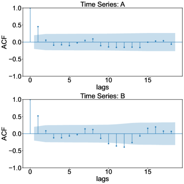
Figure 1: Autocorrelation function (ACF) of the one-step-ahead prediction residuals from two time series in the $\mathtt{m4\_hourly}$ dataset, computed using prediction results of DeepAR. The shaded area highlights the 95% confidence interval, denoting regions where the correlation is statistically insignificant.

3 RELATED WORK

3.1 Probabilistic Time Series Forecasting

Probabilistic forecasting aims to offer the predictive distribution of the target variable rather than producing a single-point estimate, as seen in deterministic forecasting. Essentially, there are two approaches to achieve this: via the probability density function (PDF) or through the quantile function (Benidis et al.,, 2022). For example, MQ-RNN (Wen et al.,, 2017) employs sequence-to-sequence (Seq2Seq) recurrent neural networks (RNNs) to directly output specific quantiles of the predictive distribution.

In contrast, PDF-based models typically use a probabilistic model to describe the distribution of the target variables, with neural networks often employed to generate the parameters of this probabilistic model. For example, DeepAR (Salinas et al.,, 2020) employs RNNs to model the transitions of hidden state. The hidden state at each time step is used to generate the parameters of a Gaussian distribution. Consequently, prediction samples for the target variables can be drawn from this distribution. GPVar (Salinas et al.,, 2019), a multivariate extension of DeepAR, utilizes a Gaussian copula to transform the original observations into Gaussian variables. Subsequently, a multivariate Gaussian distribution is assumed for these transformed variables. State space model (SSM) is also a popular choice for the probabilistic model. For instance, the deep SSM model proposed by Rangapuram et al., (2018) employs RNNs to generate parameters for the state space model, facilitating the generation of prediction samples. The Normalizing Kalman Filter (de Bézenac et al.,, 2020) combines normalizing flows with the linear Gaussian state space model. This integration enables the modeling of nonlinear dynamics using RNNs and a more flexible probability density function for observations with normalizing flows. The deep factor model (Wang et al.,, 2019) employs a deterministic model and a probabilistic model separately to capture the global and local random effects of time series. The probabilistic model could be any classical probabilistic time series model such as a Gaussian noise process. Conversely, the global model, parameterized by neural networks, is dedicated to representing the deterministic patterns inherent in time series.

Various efforts have been undertaken to improve the quality of probabilistic forecasting. One avenue involves enhancing expressive conditioning for probabilistic models. For example, some approaches involve replacing RNNs with Transformer to model latent state dynamics, thus mitigating the Markovian assumption inherent in RNNs (Tang and Matteson,, 2021). Another approach focuses on adopting more sophisticated distribution forms, such as normalizing flows (Rasul et al.,, 2020) and diffusion models (Rasul et al.,, 2021). For a recent and comprehensive review, readers are referred to Benidis et al., (2022).

3.2 Modeling Correlated Errors

Error correlation can be categorized into two main types: autocorrelation and contemporaneous correlation. In time series analysis, autocorrelation occurs when errors in a time series are correlated over different time points, while contemporaneous correlation refers to the correlation between errors at the same time step.

Autocorrelation has been extensively studied in classical time series models (Prado et al.,, 2021; Hyndman and Athanasopoulos,, 2018; Hamilton,, 2020). Statistical frameworks, including autoregressive (AR) and moving average (MA) models, have been well-developed to address autocorrelation. One important method is dynamic regression (Hyndman and Athanasopoulos,, 2018), where errors are assumed to follow an ARIMA process. Recent DL-based models have also attempted to handle autocorrelation, such as re-parameterizing the input and output of neural networks to model first-order error autocorrelation with an AR process (Sun et al.,, 2021). This method enhances the performance of DL-based time series models, and the parameters introduced to model autocorrelation can be jointly optimized with the base DL model. However, it is limited to one-step-ahead forecasting. This method was later extended to multivariate models for Seq2Seq traffic forecasting tasks by Zheng et al., (2023), assuming a matrix AR process for the matrix-valued errors.

Contemporaneous correlation modeling often appears in spatial regression tasks. For instance, Jia and Benson, (2020) proposed using a multivariate Gaussian distribution to model label correlation in the node regression problem, where the predicted label at each node is often considered conditionally independent. This correlation can later be utilized to refine predictions for unknown nodes using information from known node labels. The introduction of Generalized Least Squares (GLS) loss in Zhan and Datta, (2023) captures the spatial correlation of errors in neural networks for geospatial data, bridging deep learning with Gaussian processes. A similar approach, involving the utilization of GLS loss with random forest, was proposed by Saha et al., (2023). Contemporaneous correlation is also modeled in time series forecasting to capture the interdependence between time series. The methods range from using a parametric multivariate Gaussian distribution (Salinas et al.,, 2019) to more expressive generative models such as normalizing flows (Rasul et al.,, 2020) and diffusion models (Rasul et al.,, 2021). In Choi et al., (2022), a dynamic mixture of matrix normal distributions was proposed to characterize spatiotemporally correlated errors in multivariate Seq2Seq forecasting tasks.

To the best of our knowledge, our study presents an innovative training approach to addressing error autocorrelation in probabilistic time series forecasting. Our proposed method is closely related to those introduced in Sun et al., (2021), Zhan and Datta, (2023), and Saha et al., (2023). While Zhan and Datta, (2023), and Saha et al., (2023) primarily concentrate on modeling contemporaneous correlation, and Sun et al., (2021) focuses on modeling autocorrelation in deterministic forecasting. our method concentrates on learning temporally correlated errors in the probabilistic time series forecasting context. We utilize a dynamic covariance matrix to capture autocorrelation within a mini-batch, which is simultaneously learned alongside the base model. The introduction of the error covariance matrix not only provides a statistical framework for characterizing error autocorrelation but also enhances prediction accuracy.

4 OUR METHOD

Our approach is based on the formulation presented in Eq. (3), using an autoregressive model as the base model. Given the primary focus of this paper on univariate models, we will omit the subscript $i$ for the remainder of this paper. In a general sense, an autoregressive probabilistic forecasting model comprises two key components: firstly, a transition model (e.g., an RNN) to characterize state transitions $\mathbf{h}_{t}$, and secondly, a distribution head $\theta$ responsible for mapping $\mathbf{h}_{t}$ to the parameters governing the desired distribution. Furthermore, the encoder-decoder framework is employed to facilitate multi-step forecasting, wherein an input sequence spanning $P$ time steps is used to generate an output sequence spanning $Q$ time steps. The likelihood is expressed as $p\left(z_{t}\mid\theta(\mathbf{h}_{t})\right)$ for an individual observation, and in the case of employing a Gaussian distribution, $\theta(\mathbf{h}_{t})$ takes the form of $(\mu_{t},\sigma_{t})$. In the training batch, the target time series variable can be decomposed as

$$z_{t}=\mu_{t}+\sigma_{t}\epsilon_{t}.$$ (5)

where $\epsilon_{t}$ is the normalized error term, which usually follows the assumption that $\epsilon_{t}=\frac{z_{t}-\mu_{t}}{\sigma_{t}}\overset{\text{iid}}{\sim}\mathcal{N}(0,1)$. This assumption implies that $\epsilon_{t}$ are independent and identically distributed according to a standard normal distribution. Consequently, the parameters of the model can be optimized by maximizing its log-likelihood:

$$\mathcal{L}=\sum_{t=1}^{T}\log p\left(z_{t}\mid\theta\left(\mathbf{h}_{t}\right)\right)\propto\sum_{t=1}^{T}-\frac{1}{2}\epsilon_{t}^{2}-\ln\sigma_{t}.$$ (6)

We adopt a unified univariate model trained across all time series, rather than training individual models for each time series. Moreover, if we assume the error process to be isotropic, the loss function is equivalent to the Mean Squared Error (MSE) commonly employed in training deterministic models (Sun et al.,, 2021). However, this assumption of independence ignores the potential serial correlation in $\epsilon_{t}$.

4.1 Training with Mini-batch

We propose a novel training approach by constructing mini-batches instead of using individual training instances. For most existing deep probabilistic time series models including DeepAR, each training instance consists of a time series segment with a length of $P+Q$, where $P$ represents the conditioning range and $Q$ denotes the prediction range. However, as mentioned, this simple approach cannot characterize the serial correlation of errors among consecutive time steps. To address this issue, we group $D$ consecutive time series segments into a mini-batch, with each segment having a length of $P+1$ (i.e., $Q=1$). In other words, the new training instance (i.e., a mini-batch) becomes a collection of $D$ time series segments with a prediction range $Q=1$. The composition of a mini-batch is illustrated in Fig. 2. An example of the collection of target variables in a mini-batch of size $D$ (the time horizon we use for capturing serial correlation) is given by

$$z_{t} =\mu_{t}+\sigma_{t}\epsilon_{t},$$ (7)

$$z_{t+1} =\mu_{t+1}+\sigma_{t+1}\epsilon_{t+1},$$

$$\ldots$$

$$z_{t+D-1} =\mu_{t+D-1}+\sigma_{t+D-1}\epsilon_{t+D-1},$$

where for time point $t^{\prime}$, $\mu_{t^{\prime}}$ and $\sigma_{t^{\prime}}$ are the output of the model for each time series segment in the mini-batch, and $\epsilon_{t^{\prime}}$ is the normalized error term. We use boldface symbols to denote the vectors of data and parameters in this mini-batch, e.g., $\boldsymbol{z}_{t}^{\text{bat}}=\left[z_{t},z_{t+1},\ldots,z_{t+D-1}\right]^{\top}$ and the same notation applies to $\boldsymbol{\mu}_{t}^{\text{bat}}$ and $\boldsymbol{\sigma}_{t}^{\text{bat}}$.

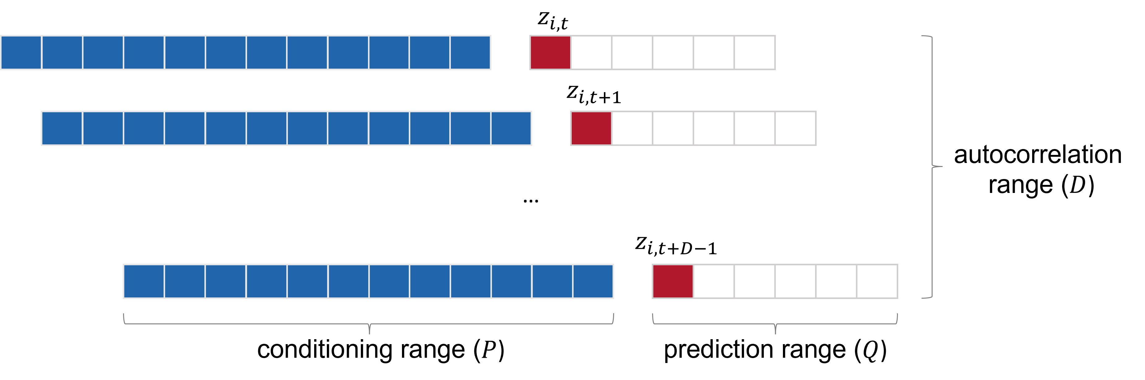
Figure 2: Example of a mini-batch. Colored parts denote the time series segments that construct the mini-batch. Each mini-batch has a time span of $P+D$, and only one-step-ahead prediction is involved during training.

Rather than assuming independence among the normalized errors, we consider modeling the joint distribution of the error vector in a mini-batch $\boldsymbol{\epsilon}_{t}$, denoted as $\boldsymbol{\epsilon}_{t}^{\text{bat}}=\left[{\epsilon}_{t},{\epsilon}_{t+1},\ldots,{\epsilon}_{t+D-1}\right]^{\top}\sim\mathcal{N}\left(\boldsymbol{0},\boldsymbol{C}_{t}\right)$, where $\boldsymbol{C}_{t}$ is a time-varying correlation matrix. To efficiently characterize the time-varying patterns, we parameterize $\boldsymbol{C}_{t}$ as a dynamic weighted sum of several base kernel matrices: $\boldsymbol{C}_{t}=\sum_{m=1}^{M}w_{m,t}\boldsymbol{K}_{m}$, where $w_{m,t}\geq 0$ (with $\sum_{m}w_{m,t}=1$) is the component weight. For each base component, we use a kernel matrix generated from a squared-exponential (SE) kernel function $\boldsymbol{K}^{ij}_{m}=\exp(-\frac{(i-j)^{2}}{l_{m}^{2}})$ with different lengthscales $l_{m}$ (e.g., $l_{m}=1,2,3,\dots$). An identity matrix is included in the additive structure to capture the independent noise process. Taken together, this parameterization ensures that $\boldsymbol{C}_{t}$ is a positive definite symmetric matrix with unit diagonals, thus being a valid correlation matrix. A small neural network is attached to the original model to project the hidden state to the weights by setting the number of nodes in the final hidden layer to $M$ (i.e., the number of components). A softmax layer is used as the output layer to ensure that these weights sum up to 1. The parameters of the small neural network can be learned jointly with the base model.

The utilization of a time-varying correlation matrix, as opposed to a static correlation matrix, offers the advantage of enabling the model to adapt dynamically to the evolving structure of the error process. For example, the model can assign a higher weight to a kernel matrix generated by a kernel function with a lengthscale of $l=3$ when strong and long-range correlations are present in the current context, whereas it can favor the identity matrix when errors become white noise. This parameterization empowers the model to capture positive autocorrelation that diminishes over time lags. Alternatively, one could opt for a fully learnable positive definite symmetric Toeplitz matrix to parameterize the correlation matrix, which can also accommodate negative and complex correlations. With this formulation, the distribution of $\boldsymbol{\epsilon}_{t}$ becomes a multivariate Gaussian, which also leads to $\boldsymbol{z}_{t}^{\text{bat}}\sim\mathcal{N}\left(\boldsymbol{\mu}_{t}^{\text{bat}},\boldsymbol{\Sigma}_{t}^{\text{bat}}\right)$. The $D\times D$ covariance of the associated target variables can be decomposed as $\boldsymbol{\Sigma}_{t}^{\text{bat}}=\operatorname{diag}(\boldsymbol{\sigma}_{t}^{\text{bat}})\boldsymbol{C}_{t}\operatorname{diag}(\boldsymbol{\sigma}_{t}^{\text{bat}})$. As both $\boldsymbol{\mu}_{t}^{\text{bat}}$ and $\boldsymbol{\sigma}_{t}^{\text{bat}}$ are default outputs of the base probabilistic model, the likelihood for a specific time series can be constructed for each mini-batch, and the overall likelihood is given by

$$\mathcal{L}=\sum_{t=1}^{T-D+1}\log p\left(\boldsymbol{z}_{t}^{\text{bat}}\mid\boldsymbol{\mu}_{t}^{\text{bat}},\boldsymbol{\Sigma}_{t}^{\text{bat}}\right).$$ (8)

By allowing overlap, a total of $T-D+1$ mini-batches can be generated for each time series from the training data.

4.2 Multi-step Rolling Prediction

An autoregressive model performs forecasting in a rolling manner by drawing a sample of the target variable at each time step, feeding it to the next time step as input, and continuing this process until the desired prediction range is reached. Our method can provide extra calibration for this process using the proposed correlation matrix $\boldsymbol{C}_{t}$. Assume that we have observations till time step $t$ and recall that the collection of normalized errors in a mini-batch jointly follows a multivariate Gaussian distribution. For the next time step $(t+1)$ to be predicted, we have the conditional distribution of $\epsilon_{t+1}$ given the past $(D-1)$ errors using the conditional distribution properties of jointly Gaussian variables:

$$\epsilon_{t+1}\mid\epsilon_{t},\epsilon_{t-1},\ldots,\epsilon_{t-D+2}\\ \sim\mathcal{N}\left(\boldsymbol{C}_{*}\boldsymbol{C}_{\text{obs}}^{-1}\boldsymbol{\epsilon}_{\text{obs}},1-\boldsymbol{C}_{*}\boldsymbol{C}_{\text{obs}}^{-1}\boldsymbol{C}_{*}^{\top}\right),$$ (9)

where $\boldsymbol{\epsilon}_{\text{obs}}=\left[\epsilon_{t-D+2},\ldots,\epsilon_{t-1},\epsilon_{t}\right]^{\top}\in\mathbb{R}^{D-1}$ represents the set of observed $(D-1)$ residuals at forecasting step $t+1$. Here, $\boldsymbol{C}_{\text{obs}}$ denotes the $(D-1)\times(D-1)$ partition of $\boldsymbol{C}_{t+1}$ that captures the correlations within $\boldsymbol{\epsilon}_{\text{obs}}$, and $\boldsymbol{C}_{*}$ denotes the $1\times(D-1)$ partition of $\boldsymbol{C}_{t+1}$ that captures the correlations between $\epsilon_{t+1}$ and $\boldsymbol{\epsilon}_{\text{obs}}$, i.e., $\boldsymbol{C}_{t+1}=\begin{bmatrix}\boldsymbol{C}_{\text{obs}}&\boldsymbol{C}_{*}^{\top}\\ \boldsymbol{C}_{*}&1\end{bmatrix}$, where the weights for generating $\boldsymbol{C}_{t+1}$ are obtained from the hidden state of the base model at time step $t+1$. Note that we remove the time index in $\boldsymbol{C}_{\text{obs}}$, $\boldsymbol{C}_{*}$ and $\boldsymbol{\epsilon}_{\text{obs}}$ for brevity. To obtain a sample of the target variable $\tilde{z}_{t+1}$, we can first draw a sample of the normalized error $\tilde{\epsilon}_{t+1}$ using Eq. (9). Since both $\mu_{t+1}$ and $\sigma_{t+1}$ are deterministic outcomes from the base model, $\tilde{z}_{t+1}$ can be derived by

$$\tilde{z}_{t+1}=\mu_{t+1}+\sigma_{t+1}\tilde{\epsilon}_{t+1}.$$ (10)

Based on Eq. (9) and Eq. (10), it can be seen that the final distribution for ${z}_{t+1}$ becomes

$$\left.z_{t+1}\mid{\bf{h}}_{t+1},\boldsymbol{\epsilon}_{\text{obs}}\right.\sim\mathcal{N}\left(\bar{\mu}_{t+1},\bar{\sigma}_{t+1}^{2}\right),$$ (11)

where

$$\bar{\mu}_{t+1}=\mu_{t+1}+\sigma_{t+1}\boldsymbol{C}_{*}\boldsymbol{C}_{\text{obs}}^{-1}\boldsymbol{\epsilon}_{\text{obs}},$$ (12)

$$\bar{\sigma}_{t+1}^{2}=\sigma_{t+1}^{2}\left(1-\boldsymbol{C}_{*}\boldsymbol{C}_{\text{obs}}^{-1}\boldsymbol{C}_{*}^{\top}\right).$$

Multi-step rolling prediction can be accomplished by treating the sample $\tilde{\epsilon}_{t+1}$ as a newly observed residual. Following this process for all subsequent time steps results in a trajectory of $\{\tilde{\epsilon}_{t+q}\}_{q=1}^{Q}$.

5 EXPERIMENTS

5.1 Datasets and Models

We apply the proposed framework to two base prediction models: DeepAR (Salinas et al.,, 2020) and an autoregressive decoder-only Transformer (i.e., the GPT model (Radford et al.,, 2018)). A Gaussian distribution head is employed to generate the distribution parameters for probabilistic forecasting based on the hidden state outputted by the model. It should be noted that our approach can be applied to other autoregressive univariate models without any loss of generality, as long as the final prediction follows a Gaussian distribution. We implemented these models using PyTorch Forecasting (Beitner,, 2020). Both models utilize input data consisting of lagged time series values from the preceding time step, accompanied by supplementary features including time of day, day of the week, global time index, and unique time series identifiers. We refer readers to the supplementary material for comprehensive information on the experiment setup.

To assess our method’s effectiveness, we conducted extensive experiments on diverse real-world time series datasets sourced from GluonTS (Alexandrov et al.,, 2020, please refer to supplementary material for dataset details). These datasets serve as important benchmarks in evaluating time series forecasting models. The prediction range ($Q$) and the number of rolling evaluations were acquired from each dataset’s configuration within GluonTS. Sequential splits into training, validation, and testing sets were performed for each dataset, with the validation set’s temporal length matching that of the testing sets. The temporal length of the testing set was computed using the prediction range and the number of rolling evaluations. For example, the testing set for $\mathtt{traffic}$ contains $24+7-1=30$ time steps, indicating 24-step predictions ($Q$) made in a rolling manner across 7 consecutive prediction start timestamps. Standardization of the data was carried out using the mean and standard deviation obtained from each time series within the training set. Predictions were subsequently rescaled to their original values for computing evaluation metrics.

5.2 Evaluation against Baseline

Table 1: Comparison of accuracy using the $\operatorname{CRPS}_{\text{sum}}$ metric (lower values indicate better performance and are highlighted in bold). “w/o” denotes the original model implementation optimized with Gaussian likelihood loss, while “w/” indicates the model enhanced with our method. Mean and standard deviation were calculated from three runs of each model.

	DeepAR			Transformer
	w/o	w/	rel. impr.	w/o	w/	rel. impr.
$\mathtt{m4\_hourly}$	0.1529$\pm$0.0011	0.1421$\pm$0.0003	7.06%	0.1487$\pm$0.0011	0.1431$\pm$0.0009	3.77%
$\mathtt{exchange\_rate}$	0.0069$\pm$0.0001	0.0059$\pm$0.0000	14.49%	0.0081$\pm$0.0001	0.0074$\pm$0.0001	8.64%
$\mathtt{m1\_quarterly}$	0.3767$\pm$0.0006	0.3076$\pm$0.0018	18.34%	0.4449$\pm$0.0034	0.3302$\pm$0.0046	25.78%
$\mathtt{pems03}$	0.0870$\pm$0.0000	0.0811$\pm$0.0000	6.78%	0.0907$\pm$0.0000	0.0845$\pm$0.0001	6.84%
$\mathtt{pems08}$	0.0650$\pm$0.0001	0.0588$\pm$0.0000	9.54%	0.0622$\pm$0.0000	0.0591$\pm$0.0001	4.98%
$\mathtt{solar}$	0.7627$\pm$0.0008	0.7063$\pm$0.0005	7.39%	0.6657$\pm$0.0010	0.5379$\pm$0.0010	19.20%
$\mathtt{traffic}$	0.2765$\pm$0.0001	0.2387$\pm$0.0001	13.67%	0.2422$\pm$0.0002	0.2036$\pm$0.0001	15.94%
$\mathtt{uber\_daily}$	0.0897$\pm$0.0003	0.0890$\pm$0.0001	0.78%	0.0827$\pm$0.0003	0.0827$\pm$0.0002	0.00%
$\mathtt{uber\_hourly}$	0.1549$\pm$0.0007	0.1532$\pm$0.0005	1.10%	0.1503$\pm$0.0007	0.1462$\pm$0.0008	2.73%
		avg. rel. impr.	8.80%		avg. rel. impr.	9.76%

We evaluate the proposed approach by comparing it with models trained using Gaussian likelihood loss. To simplify the comparison and ensure fairness in terms of the data used during training, we set the autocorrelation range ($D$) to be identical to the prediction range ($Q$). This alignment ensures that each mini-batch in our method covers a time horizon of $P+D$, while in the conventional training method, each training instance spans a time horizon of $P+Q$. By setting $D=Q$, we guarantee that both methods involve the same amount of data per batch, given the same batch sizes. Furthermore, we follow the default configuration in GluonTS by setting the context range equal to the prediction range, i.e., $P=Q$.

In our proposed method, we introduce a small number of additional parameters dedicated to projecting the hidden state into component weights $w_{m,t}$, which play a pivotal role in generating the dynamic correlation matrix $\boldsymbol{C}_{t}$. In practice, the selection of base kernels should be data-specific, and one should perform residual analysis to determine the most appropriate structure. For simplicity, we use $M=4$ base kernels—three SE kernels with $l=1,2,3$, respectively, and an identity matrix. The different lengthscales capture different decaying rates of autocorrelation. The time-varying component weights can help the model dynamically adjust to different correlation structures observed at different time points. We use the Continuous Ranked Probability Score (CRPS) (Gneiting and Raftery,, 2007) as the evaluation metric for uncertainty quantification:

$$\operatorname{CRPS}(F,y)=\mathbb{E}_{F}|Y-y|-\frac{1}{2}\mathbb{E}_{F}\left|Y-Y^{\prime}\right|,$$ (13)

where $y$ is the observation, $F$ is the cumulative distribution function (CDF) of a random variable $Y$, which is the target time series variable $z_{t}$ in our case. For a clearer demonstration, we use $\operatorname{CRPS}_{\text{sum}}$ calculated by first summing $\operatorname{CRPS}$ across the entire testing horizon of all time series and then normalizing the result by the sum of the corresponding observations. Detailed information on the calculation of the CRPS is available in the supplementary materials.

In Table 1, we present a comparative analysis of prediction performance using DeepAR and Transformer as base models. The variants combined with our proposed method are compared to their respective original implementations optimized with Gaussian likelihood loss. The results demonstrate the effectiveness of our approach in enhancing the performance of both models across a wide range of datasets, yielding notable improvements in predictive accuracy. Our method yields an average improvement of 8.80% for DeepAR and 9.76% for Transformer. It should be noted that our method exhibits versatile performance improvements that vary across different datasets. This variability can be attributed to a combination of factors, including the inherent characteristics of the data and the baseline performance of the original model on each specific dataset. Notably, when the original model already achieves exceptional performance on a particular dataset, our method could demonstrate minimal enhancement (e.g., $\mathtt{uber\_daily}$ and $\mathtt{uber\_hourly}$). Moreover, the degree of alignment between our kernel assumption and the true error autocorrelation structure significantly impacts the performance of our method. Further analyses with other evaluation metrics (e.g. MSE and quantile loss) are reported in supplementary material.

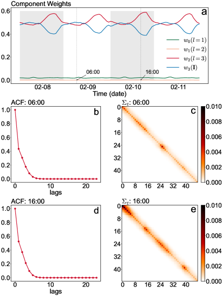
Figure 3: (a) Component weights for generating the correlation matrix of an example time series from the $\mathtt{m4\_hourly}$ dataset. Parameters $w_{0},w_{1},w_{2}$ represent the component weights for kernel matrices associated with lengthscales $l=1,2,3$, respectively, and $w_{3}$ is the component weight for the identity matrix. Shaded areas distinguish different days; (b) and (d): The autocorrelation function (ACF) indicated by the resulting error correlation matrix $\boldsymbol{C}_{t}$ at 6:00 and 16:00. Given the rapid decay of the ACF, we only plot 24 lags to enhance clarity in our visualization; (c) and (e): The corresponding covariance matrix of the associated target variables $\boldsymbol{\Sigma}_{t}=\operatorname{diag}(\boldsymbol{\sigma}_{t})\boldsymbol{C}_{t}\operatorname{diag}(\boldsymbol{\sigma}_{t})$ at 6:00 and 16:00, respectively.

5.3 Interpretation of Correlation

A key element of our method lies in its ability to capture error autocorrelation through the dynamic construction of a covariance matrix. This is achieved by introducing a dynamic weighted sum of kernel matrices with different lengthscales. The choice of lengthscale significantly influences the structure of autocorrelation—a small lengthscale corresponds to short-range positive autocorrelation, while a large lengthscale can capture positive correlation spanning long lags.

In Fig. 3, we present the generated component weights and the resulting autocorrelation function (i.e., the first row in the learned correlation matrix $\boldsymbol{C}_{t}$) of an example time series from the $\mathtt{m4\_hourly}$ dataset over a four-day duration. In particular, we observe that the component weights ($w_{0},w_{1}$), corresponding to the kernel matrices with $l=1$ and $l=2$, consistently remain close to zero across the entire observation period. This suggests that the prevailing autocorrelation structure in this dataset is most effectively characterized by the kernel matrix associated with $l=3$.

Furthermore, we observe the dynamic adjustment of correlation strengths facilitated by the identity matrix over time. Specifically, when $w_{3}$ (weight assigned to the identity matrix) increases, the error process tends to exhibit greater independence. In contrast, when the weight $w_{2}$ for the kernel matrix with $l=3$ is larger, the error process becomes more correlated. Figs. 3 (b, d) reveal that the autocorrelation at 6:00 in the morning is less pronounced compared to that observed at 16:00. Additionally, Fig. 3 (a) demonstrates pronounced daily patterns in autocorrelation, particularly when errors exhibit an increased correlation around 18:00 each day. This underscores the crucial need for our methodology to dynamically adapt the covariance matrix, enabling the effective modeling of these temporal variations. Figs. 3 (c, e) depict the covariance matrix of the respective target variables within the autocorrelation horizon. The diagonal elements represent the variance of the target variables generated by the base model, while the off-diagonal elements depict the covariance of the target variables that are facilitated by our approach.

6 CONCLUSION

This paper introduces an innovative training approach to model error autocorrelation in probabilistic time series forecasting. The method involves using mini-batches in training and learning a time-varying covariance matrix that captures the correlation among normalized errors within a mini-batch. Taken together with the standard deviation provided by the base model, we are able to model and predict a time-varying covariance matrix. We implement and evaluate the proposed method using DeepAR and Transformer on various public datasets, and our results confirm the effectiveness of the proposed solution in improving the quality of uncertainty quantification. The broader impact of our method can be observed in two aspects. First, since Gaussian errors are commonly assumed in probabilistic forecasting models, our method can be applied to enhance the training process of such models. Second, the learned autocorrelation can be leveraged to improve multi-step prediction by calibrating the distribution output at each forecasting step.

There are several directions for future research. First, the kernel-based covariance matrix may be too restrictive for capturing temporal processes. Investigating covariance structures with greater flexibility, such as parameterizing $\boldsymbol{C}_{t}$ as a fully learnable positive definite symmetric Toeplitz matrix (e.g., AR($p$) process has covariance with a Toeplize structure) and directly factorizing the covariance matrix $\boldsymbol{\Sigma}_{t}=\boldsymbol{U}_{t}\boldsymbol{U}_{t}^{\top}$ (e.g., Wishart process as in Wilson and Ghahramani, (2011)) or the precision matrix $\boldsymbol{\Lambda}_{t}=\boldsymbol{\Sigma}_{t}^{-1}=\boldsymbol{V}_{t}\boldsymbol{V}_{t}^{\top}$ (e.g., using Cholesky factorization as in Fortuin et al., (2020)), could be promising avenues. Second, our method can be extended to multivariate models, in which the target output becomes a vector instead of a scalar. A possible solution is to use a matrix Gaussian distribution to replace the multivariate Gaussian distribution used in the current method. This would allow us to learn a full covariance matrix between different target series, thereby capturing any cross-correlations between them.

References

- Alexandrov et al., (2020) Alexandrov, A., Benidis, K., Bohlke-Schneider, M., Flunkert, V., Gasthaus, J., Januschowski, T., Maddix, D. C., Rangapuram, S., Salinas, D., Schulz, J., et al. (2020). Gluonts: Probabilistic and neural time series modeling in python. The Journal of Machine Learning Research, 21(1):4629–4634.
- Beitner, (2020) Beitner, J. (2020). Pytorch forecasting. https://pytorch-forecasting.readthedocs.io.
- Benidis et al., (2022) Benidis, K., Rangapuram, S. S., Flunkert, V., Wang, Y., Maddix, D., Turkmen, C., Gasthaus, J., Bohlke-Schneider, M., Salinas, D., Stella, L., et al. (2022). Deep learning for time series forecasting: Tutorial and literature survey. ACM Computing Surveys, 55(6):1–36.
- Choi et al., (2022) Choi, S., Saunier, N., Trepanier, M., and Sun, L. (2022). Spatiotemporal residual regularization with dynamic mixtures for traffic forecasting. arXiv preprint arXiv:2212.06653.
- de Bézenac et al., (2020) de Bézenac, E., Rangapuram, S. S., Benidis, K., Bohlke-Schneider, M., Kurle, R., Stella, L., Hasson, H., Gallinari, P., and Januschowski, T. (2020). Normalizing kalman filters for multivariate time series analysis. Advances in Neural Information Processing Systems, 33:2995–3007.
- Fortuin et al., (2020) Fortuin, V., Baranchuk, D., Rätsch, G., and Mandt, S. (2020). Gp-vae: Deep probabilistic time series imputation. In International conference on artificial intelligence and statistics, pages 1651–1661. PMLR.
- Gneiting and Raftery, (2007) Gneiting, T. and Raftery, A. E. (2007). Strictly proper scoring rules, prediction, and estimation. Journal of the American statistical Association, 102(477):359–378.
- Hamilton, (2020) Hamilton, J. D. (2020). Time Series Analysis. Princeton University Press.
- Hyndman and Athanasopoulos, (2018) Hyndman, R. J. and Athanasopoulos, G. (2018). Forecasting: Principles and Practice. OTexts.
- Jia and Benson, (2020) Jia, J. and Benson, A. R. (2020). Residual correlation in graph neural network regression. In Proceedings of the 26th ACM SIGKDD International Conference on Knowledge Discovery & Data Mining, pages 588–598.
- Prado et al., (2021) Prado, R., Ferreira, M. A., and West, M. (2021). Time Series: Modeling, Computation, and Inference. CRC Press.
- Radford et al., (2018) Radford, A., Narasimhan, K., Salimans, T., Sutskever, I., et al. (2018). Improving language understanding by generative pre-training.
- Rangapuram et al., (2018) Rangapuram, S. S., Seeger, M. W., Gasthaus, J., Stella, L., Wang, Y., and Januschowski, T. (2018). Deep state space models for time series forecasting. Advances in neural information processing systems, 31.
- Rasul et al., (2021) Rasul, K., Seward, C., Schuster, I., and Vollgraf, R. (2021). Autoregressive denoising diffusion models for multivariate probabilistic time series forecasting. In International Conference on Machine Learning, pages 8857–8868. PMLR.
- Rasul et al., (2020) Rasul, K., Sheikh, A.-S., Schuster, I., Bergmann, U., and Vollgraf, R. (2020). Multivariate probabilistic time series forecasting via conditioned normalizing flows. arXiv preprint arXiv:2002.06103.
- Saha et al., (2023) Saha, A., Basu, S., and Datta, A. (2023). Random forests for spatially dependent data. Journal of the American Statistical Association, 118(541):665–683.
- Salinas et al., (2019) Salinas, D., Bohlke-Schneider, M., Callot, L., Medico, R., and Gasthaus, J. (2019). High-dimensional multivariate forecasting with low-rank gaussian copula processes. Advances in neural information processing systems, 32.
- Salinas et al., (2020) Salinas, D., Flunkert, V., Gasthaus, J., and Januschowski, T. (2020). Deepar: Probabilistic forecasting with autoregressive recurrent networks. International Journal of Forecasting, 36(3):1181–1191.
- Sun et al., (2021) Sun, F.-K., Lang, C., and Boning, D. (2021). Adjusting for autocorrelated errors in neural networks for time series. Advances in Neural Information Processing Systems, 34:29806–29819.
- Tang and Matteson, (2021) Tang, B. and Matteson, D. S. (2021). Probabilistic transformer for time series analysis. Advances in Neural Information Processing Systems, 34:23592–23608.
- Wang et al., (2019) Wang, Y., Smola, A., Maddix, D., Gasthaus, J., Foster, D., and Januschowski, T. (2019). Deep factors for forecasting. In International conference on machine learning, pages 6607–6617. PMLR.
- Wen et al., (2017) Wen, R., Torkkola, K., Narayanaswamy, B., and Madeka, D. (2017). A multi-horizon quantile recurrent forecaster. arXiv preprint arXiv:1711.11053.
- Wilson and Ghahramani, (2011) Wilson, A. G. and Ghahramani, Z. (2011). Generalised wishart processes. In Proceedings of the Twenty-Seventh Conference on Uncertainty in Artificial Intelligence, pages 736–744.
- Zhan and Datta, (2023) Zhan, W. and Datta, A. (2023). Neural networks for geospatial data. arXiv preprint arXiv:2304.09157.
- Zheng et al., (2023) Zheng, V. Z., Choi, S., and Sun, L. (2023). Enhancing deep traffic forecasting models with dynamic regression. arXiv preprint arXiv:2301.06650.