Asynchronous Multiple LiDAR-Inertial Odometry
using Point-wise Inter-LiDAR Uncertainty Propagation

Abstract

In recent years, multiple LiDAR (LiDAR) systems have grown in popularity due to their enhanced accuracy and stability from the increased FOV (FOV). However, integrating multiple LiDARs can be challenging, attributable to temporal and spatial discrepancies. Common practice is to transform points among sensors while requiring strict time synchronization or approximating transformation among sensor frames. Unlike existing methods, we elaborate the inter-sensor transformation using CT (CT) IMU (IMU) modeling and derive associated ambiguity as a point-wise uncertainty. This uncertainty, modeled by combining the state covariance with the acquisition time and point range, allows us to alleviate the strict time synchronization and to overcome FOV difference. The proposed method has been validated on both public and our datasets and is compatible with various LiDAR manufacturers and scanning patterns. We open-source the code for public access at https://github.com/minwoo0611/MA-LIO.

I INTRODUCTION & RELATED WORKS

Over the last decades, robot navigation using LiDAR has made substantial advances in localization and map construction. Although existing methods mostly solve for a single LiDAR system, limited FOV and occlusion lead to a need for multiple LiDARs. When integrating multiple LiDARs in a complementary configuration, two major challenges impede naive integration, namely temporal and spatial discrepancy.

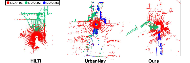
(a) Multi-LiDAR datasets

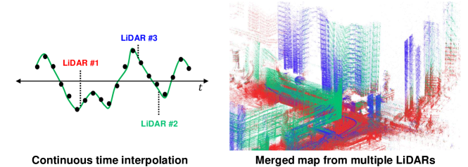
(b) Constructed map using multi-LiDAR

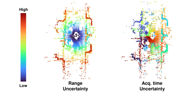
(c) Two types of uncertainties

Figure 1: (a) Example of FOV difference in multi-LiDAR datasets (b) CT IMU interpolation enable us to merge points accurately, thus substantially increasing net FOV in the accumulated map. (c) Two types of uncertainties considered in this paper.

(i) Synchronization: It is straightforward and enticing to secure strict time synchronization among sensors to obtain all measurements at the same time for easy integration. M-LOAM [1] proposed the multiple LiDAR odometry for carefully synchronized LiDAR. In practice, sensors can be synchronized by PPS (PPS) via external hardware for transmitting the PPS signal. Another option is PTP (PTP), yet not all manufacturers support it, thus requiring sensor combinations made by the same manufacturers.

Due to this sophisticated setting for synchronization, some asynchronous public datasets [2, 3, 4, 5] require software solutions to handle temporal discrepancies. For example, LOCUS [6] assumed synchronization to merge pointclouds. Later in LOCUS 2.0 [5], they discarded delayed scans for improved robustness accepting induced information loss. Lin et al. [7] applied decentralized Extended Kalman Filter for asynchronous Livox LiDARs; however, their small FOV could induce the error in degenerate environments when processing each LiDAR separately. Nguyen et al. [8] and Wang et al. [9] exploited the IMU to compensate for temporal discrepancies. The idea of utilizing IMU was affordable; still, the error originating from discrete propagation remains. Some researchers suggested using optimization in continuous-time formulation [10, 11]. While this approach can estimate the entire trajectory at any point in time, intensive computational burden hindered real-time feasibility.

In contrast, our method utilizes all available information, including asynchronous scans, and avoiding linear approximation. We decided not to include the continuous term in the optimization phase for a real-time process. Instead, B-Spline interpolation is leveraged to estimate the trajectory for each LiDAR measurement, enabling a computationally efficient solution for multi-LiDAR SLAM in real-world environments.

(ii) Spatial discrepancy: Another solution for this temporal discrepancy is to apply scan matching and compute necessary correction. However, spatial discrepancy induced from different scanning patterns and FOV among LiDARs hinders scan matching in overcoming the temporal discrepancy. Specifically, sparsity and FOV variance from non-repetitive scanning patterns [2] and obliquely installed spinning pattern [3], may yield a little overlapping area among sensors.

(iii) Uncertainty propagation: From both temporal and spatial discrepancy, we inevitably accumulate ambiguity during the projection of the points among sensors. Regarding this issue, proper uncertainty modeling could capture the transferred ambiguity among multiple LiDARs. The usage of uncertainty in LiDAR has been extensively studied in recent years, mostly focusing on learning-based methods [12, 13, 14, 15].

Yet, like ours, some model-based approaches have been presented. For example, Wang et al. [9] calculated the weight for LiDAR residual based on the difference between IMU and LiDAR odometry. Whereas all points were treated equally in [9], we assign point-wise uncertainty by considering their range and acquisition time. This is particularly important to handle both ambiguities induced by the temporal and spatial discrepancy. M-LOAM [1] propagated the uncertainty in each point by using the extrinsic covariance and the state covariance. This approach is similar to ours in that utilizing state covariance and point-wise uncertainty propagation [16]. Differing from M-LOAM, our method requires no inter-LiDAR overlap for extrinsic covariance update and thus is more generic in handling point-level uncertainty. In [17], authors considered the variance of normal direction using uncertainty to deal with the uneven terrain but without incorporating acquisition time and range ambiguity.

Differing from the existing methods, this paper proposes an asynchronous multiple LiDAR-inertial odometry (Fig. 2). To deal with the abovementioned challenges in multi-LiDAR, we model point-wise uncertainty by considering the range and state covariance at each time. Furthermore, we calculate localization weight using the surrounding environment to determine the weight term during optimization. Handling a large number of points efficiently, we exploit ikd-Tree [18] and an IESKF (IESKF), achieving computational efficiency. Our contributions are as follows:

1. We tackle FOV discrepancy by accurately transferring points among LiDARs, which the scan matching approach failed to solve. Furthermore, by utilizing CT B-spline interpolation, we reduce temporal discrepancy, thus yielding consistency in inter-LiDAR scan alignment even with a significant FOV difference.

2. The proposed point-level uncertainty captures increased ambiguity induced by range and point acquisition time. This point-wise assessment assigns larger uncertainty for points farther in range or later in time, hence handling uncertainty more generically.

3. The proposed localization weight balances the ratio between prior and measurement residual during optimization. This enables to automatic adapt the proportion of each residual in degenerate environments such as tunnels and narrow corridors.

4. Our method is validated on public and our own datasets. It is compatible with any combination of LiDAR with different scanning patterns from various manufacturers.

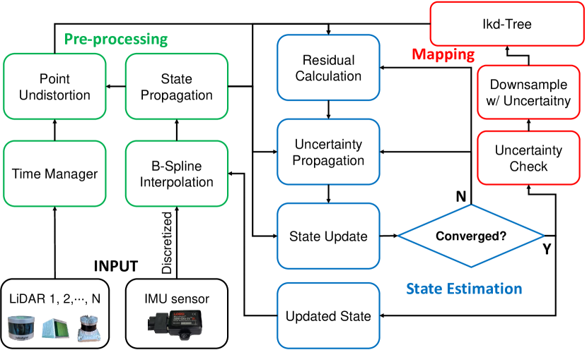
Figure 2: The proposed method consists of three modules: preprocessing, state estimation, and mapping. In the preprocessing stage, the points from each LiDAR are corrected for distortion and merged by B-spline interpolation. The state estimation stage involves point-wise uncertainty propagation and the application of an IESKF until convergence is achieved. Finally, the optimal state is passed to the IMU model for accurate interpolation in subsequent scans. The data points are projected into ikd-Tree after assessing their uncertainty.

II METHOD

II-A The Notion and State

Subscript $A$ in notation $()_{A}$ denotes the representing frame. The frame $B$ in frame $A$ is denoted as $()_{AB}$. The ground truth is represented as $()$, while propagated, error, and optimal state are denoted as $\widehat{()}$, $\tilde{()}$, and $\mathrm{bar}{()}$. For simplicity, we classify $N$ LiDARs as $\{L_{i},i=1,\cdots,N\}$, designating the LiDAR with the latest sample point as $P$ and all other LiDARs as $S$. Our system comprises a state x, input u, and noise w as

$$\mathcal{M} \triangleq SO(3)\times\mathbb{R}^{15}\times\,\Pi_{i=1}^{N}\left(SO(3)\times\mathbb{R}^{3}\right)$$

x $$\triangleq [\textbf{R}_{GI}^{T}\quad\textbf{t}_{GI}^{T}\quad\textbf{v}_{GI}^{T}\quad\textbf{b}_{\omega}^{T}\quad\textbf{b}_{a}^{T}\quad\textbf{g}_{G}^{T}\quad\textbf{R}_{IL_{i}}^{T}\quad\textbf{t}_{IL_{i}}^{T}]^{T}\in\mathcal{M}$$

u $$\triangleq \left[\omega_{m}^{T}\quad a_{m}^{T}\right]^{T},\,\textbf{w}\triangleq\left[n_{\omega}^{T}\quad n_{a}^{T}\quad n_{b\omega}^{T}\quad n_{ba}^{T}\right]^{T}.$$ (1)

For the state x, transformation of the IMU frame (denoted as $I$) in the global frame (denoted as $G$) is $\textbf{T}_{GI}=\left(\textbf{R}^{T}_{GI},\textbf{t}^{T}_{GI}\right)$, which consists of the rotation and translation. Additionally, v, g, and b stand for velocity, bias, and gravity, while $\textbf{T}_{IL}$ denote the extrinsic between LiDAR and IMU. $\{\omega_{m},a_{m}\}$ denotes the angular velocity and linear acceleration from IMU sensor. Finally, w contains the white noise of these variables.

II-B IMU Discrete Model with B-Spline Interpolation

The CT kinematic model can be converted into a discrete model using the $\boxplus$ outlined in [18] as

$$\textbf{x}_{i+1} = \textbf{x}_{i}\boxplus\left(\Delta\textnormal{t}\textbf{f}\left(\textbf{x}_{i},\textbf{u}_{i},\textbf{w}_{i}\right)\right),$$ (2)

$$\textbf{f}\left(\textbf{x},\textbf{u},\textbf{w}\right) = \begin{bmatrix}\omega_{m}-b_{\omega}-n_{\omega}\\ {\textbf{v}}_{GI}+\frac{1}{2}\left({\textbf{R}}_{GI}\left(a_{m}-b_{a}-n_{a}\right)+\textbf{g}_{G}\right)\Delta\textnormal{t}\\ {\textbf{R}}_{GI}\left(a_{m}-b_{a}-n_{a}\right)+\textbf{g}_{G}\\ n_{b\omega}\\ n_{ba}\\ 0_{3\times 1}\\ 0_{3\times{2N}}\end{bmatrix}$$

Here, the function f describes the state of the system to its subsequent state and is parameterized by the discretization interval $\Delta\textnormal{t}$. During the time interval between $(i-1)$ and $(i)^{\text{th}}$ scans, the system estimates the trajectory using the IMU, assuming the $(i-1)^{\text{th}}$ state to be optimal.

$$\widehat{\textbf{x}}_{k+1} = \widehat{\textbf{x}}_{k}\boxplus\left(\Delta\textnormal{t}\textbf{f}\left(\widehat{\textbf{x}}_{k},\textbf{u}_{k},\textbf{0}\right)\right);\,\widehat{\textbf{x}}_{0}=\mathrm{bar}{\textbf{x}}_{i-1}$$ (3)

$$\widehat{\Sigma}_{k+1} = \textbf{F}_{\tilde{\textbf{x}}_{k}}\widehat{\Sigma}_{k}\textbf{F}^{T}_{\tilde{\textbf{x}}_{i}}+\textbf{F}_{\textbf{w}_{k}}\textbf{Q}_{k}\textbf{F}^{T}_{{\textbf{w}}_{i}};\,\widehat{\Sigma}_{0}=\mathrm{bar}{\Sigma}_{i-1},$$ (4)

, where $Q_{k}$ denotes the covariance of $w_{k}$ while the jacobians $\textbf{F}_{\tilde{x}_{k}}$ and $\textbf{F}_{w_{k}}$ represent the derivatives of $\delta\left(\textbf{x}_{k+1}\boxminus\widehat{\textbf{x}}_{k+1}\right)$ with respect to each subscript, under the conditions that $(\tilde{\textbf{x}}_{k},w_{k})=(0,0)$. Also, $\widehat{\textbf{x}}_{k-1}$ can be achieved using the $\boxminus$ operator as detailed in [19]. The accuracy of the interpolation is directly dependent on the accuracy of the discrete model. Since the IMU discrete model before optimization may not be accurate, the IMU state preceding $\mathrm{bar}{\textbf{x}}_{i-1}$ is recalculated via $\boxminus$ operator.

Based on this propagation, B-spline interpolation is performed utilizing four transformations in the world frame, known as control points from $\textbf{T}^{k-1}_{GI}$ to $\textbf{T}^{k+2}_{GI}$ [11]. By this interpolation, the trajectory at any time can be estimated, which is especially beneficial for asynchronous sensor systems. Furthermore, it is highly effective in environments with curved trajectories due to smoothness of spline. The system estimates the transformation at any time $t\in[t_{k},t_{k+1})$ using

$${}^{B}\textbf{T}_{GI}\left(s\left(t\right)\right)=\textbf{T}^{k-1}_{GI}\Pi^{3}_{n=1}\exp\left(\tilde{\textbf{B}}_{j}\left(\mathrm{s}\left(t\right)\right)\Omega_{k+n-1}\right),$$ (5)

, while $t_{k}=k\Delta t$ with $\Delta t=t_{k+1}-t_{k}$, and $s(t)=\left(t-t_{k}\right)/\Delta t$. $\Omega_{k}$ denotes the incremental control pose which is calculated as $\Omega_{k}=\log\left(\left(\textbf{T}^{k-1}_{GI}\right)^{-1}\textbf{T}^{k}_{GI}\right)$. $\tilde{\textbf{B}}_{j}$ is the matrix that includes the square term of $s$, and notation ${}^{B}\textbf{T}$ means that it is calculated by B-spline. Lastly, to obtain the covariance calculated in (4), $\widehat{\Sigma}_{k+1}$ is assigned to the transformation achieved at $t\in[t_{k},t_{k+1})$. The overall process is illustrated in Fig. 3.

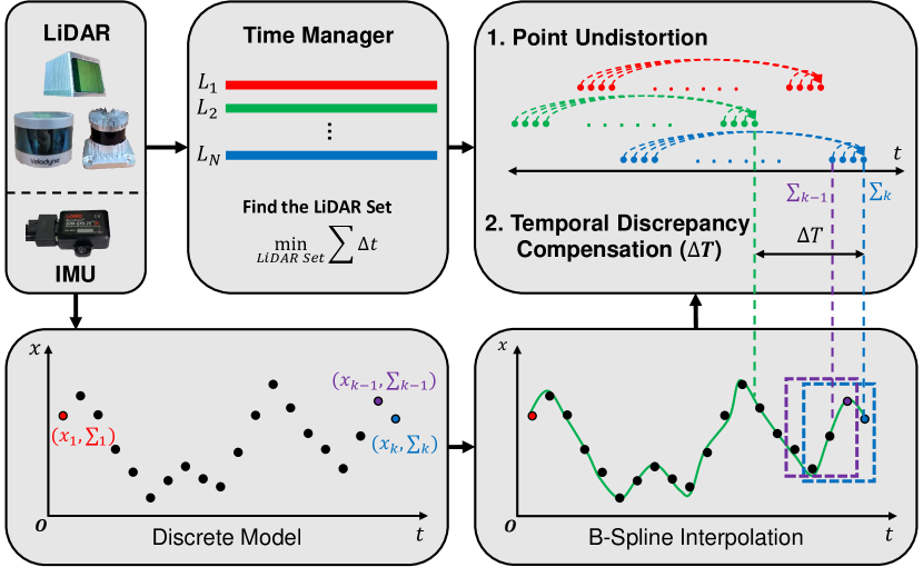
Figure 3: IMU inputs are propagated by a discrete model and fed into B-spline interpolation. We search the LiDAR that satisfies the minimal time differences. Based on the interpolation, (i) a pointcloud from LiDAR is undistorted by transformed into a single frame (the last point) and (ii) the temporal discrepancy is compensated by the relative transformation among the last points in each LiDAR.

II-C Preprocessing of Multi-LiDAR System

Despite the strict interpolation, the interpolated pose accuracy is directly affected by the minimum difference in arrival times among LiDARs. Therefore, a set of LiDAR is chosen to minimize the sum of differences in the arrival times.

For undistortion, we focus on a single LiDAR, $S$, applying the same process to others. The first step of distortion starts with merging points obtained at different times into a single frame. This is achieved by determining the relative transformation between frames. Previous studies have utilized approximate discretized IMU or linear interpolation for the inference. Instead, by using B-spline based interpolation, the point $p_{S^{j}}$ at time $t_{j}$ can be transformed to the frame at $t_{l}$ to obtain undistorted point $p^{u}_{S^{j}}$ as

$$p^{u}_{S^{j}}=\textbf{T}_{IS}^{-1}{}^{B}\textbf{T}_{{I^{l}I^{j}}}\textbf{T}_{IS}p_{S^{j}},$$ (6)

, where $t_{l}$ is the latest arrival time in $S$, and undistorted point is identified by notation $u$. Every LiDAR has different arrival times, and the temporal discrepancies should be compensated individually. When merging, the latest arrival time ($t_{i}$) of the latest LiDAR (P, denoted as blue point in Fig. 3) is leveraged to transform points acquired by other LiDARs.

$$p_{P^{i}S^{j}}=\textbf{T}_{IP}^{-1}{}^{B}\textbf{T}_{{I^{i}I^{l}}}\textbf{T}_{IS}p^{u}_{S^{j}}=\textbf{T}_{IP}^{-1}{}^{B}\textbf{T}_{{I^{i}I^{j}}}\textbf{T}_{IS}p_{S^{j}}.$$ (7)

This transformation incorporates both undistortion and temporal compensation over multiple frame changes, and errors associated with these changes may be accumulated.

II-D Uncertainty Propagation

This uncertainty must be propagated to each point using the covariance to include the errors in the optimization. Covariances of ${{}^{B}}\textbf{T}$ and $\textbf{T}_{IL}$ are achieved by (4) and IESKF. Also, the covariance of inverse transformation is calculated through $\Sigma_{inv}=\mathit{T}\Sigma\mathit{T}^{T}$, where $\mathit{T}$ is the adjoint matrix of $\textbf{T}^{-1}$. With fourth-order approximation, the transformation and covariance can be combined into $\{\textbf{T}_{{P^{i}}{S^{j}}},\Sigma_{{P^{i}}{S^{j}}}\}$ [16]. The trace of $\Sigma_{{P^{i}}{S^{j}}}$ is referred to as the acquisition time uncertainty, which is visualized in Fig. 1.

Three critical improvements beyond previous studies are as follows. Firstly, we distinguish the uncertainty according to the point sampling time, in contrast to assuming the same uncertainty in [1]. Doing so allows a more accurate uncertainty modeling associated with each point. Secondly, the specification of the primary sensor is no longer needed. In [1], because extrinsic covariance is only combined in the secondary LiDAR, the covariance of the secondary LiDAR is always higher than that of the primary LiDAR. Unlike theses, ours is more generic without specifying the primary explicitly. We utilize extrinsic covariances between LiDAR and IMU, resulting in all of the covariances being combined with the extrinsic covariance. This yields the covariances being equally affected by the extrinsic covariance. Finally, in contrast to the [1], which propagates uncertainty in the global frame, our approach propagates uncertainty on a per-point basis by confining it to the LiDAR frame. This decision aimed to account for the uncertainty introduced when fusing individual LiDAR points. By transforming a point into the frame $P$, the transformed point is presented as

$$p_{P^{i}S^{j}} \triangleq \widehat{\textbf{T}}_{{P^{i}}{S^{j}}}\widehat{p}_{S^{j}}=\exp\left(\xi^{\wedge}_{{P^{i}}{S^{j}}}\right)\textbf{T}_{{P^{i}}{S^{j}}}\left({p}_{S^{j}}+D\zeta\right)$$

$$\approx \left(I+\xi^{\wedge}_{{P^{i}}{S^{j}}}\right)\textbf{T}_{{P^{i}}{S^{j}}}\left({p}_{S^{j}}+D\zeta\right)$$

Here, $\xi$ is the error of the transformation and $\zeta\in\mathbb{R}^{3}$ is the perturbation of the LiDAR measurement. Also, $p$ in (II-D) is a $4\times 1$ vector with a scale value $1$ added, and $D$ is the dilation matrix which transforms the dimension from $3\times 1$ to $4\times 1$, with zero terms added. As the second-order error is computationally expensive but has a relatively small effect, we only consider the first-order term, $\widehat{\textbf{T}}\widehat{p}\approx\textbf{q}+\textbf{Q}\theta$.

q $$:=\textbf{T}p,\ \textbf{Q}:=\left[\left(\textbf{T}p\right)^{\odot}\ \textbf{T}D\right],\ \begin{bmatrix}\epsilon\\ \eta\end{bmatrix}^{\odot}:=\begin{bmatrix}\eta\textbf{1}\quad-\epsilon^{\wedge}\\ \textbf{0}^{T}\quad\quad\textbf{0}^{T}\end{bmatrix}$$

$$\theta :=\left[\xi^{T}\quad\zeta^{T}\right]^{T},\ \theta\sim\mathcal{N}\left(\textbf{0},\Xi\right),\ \Xi=\textnormal{diag}\left(\Sigma_{P^{i}S^{j}},\textbf{Z}\right),$$

with the LiDAR measurement covariance Z. Since $p_{P^{i}S^{j}}$ follows the Gaussian distribution, the uncertainty of the point can be obtained through (II-D), as $\Sigma_{p}=Q\Xi Q^{T}$. The resulting uncertainty is derived from the range of point $p$ from $\left(\textbf{T}p\right)^{\odot}$, and the acquisition time from $\Sigma_{P^{i}S^{j}}$. Improved accuracy is achieved by addressing ambiguity from IMU discrete model error over time and noise effects which increase with range from vibration. It is utilized for the optimization with $p_{S^{j}}$.

II-E Measurement Model with Uncertainty

Our system utilizes a surface measurement model without feature extraction under the assumption of local planarity. The points, $\{\textbf{p}_{S^{j}},j=1,\cdots,l\}$ in the LiDAR frame can be transformed to the world frame with the following equation:

$$\textbf{p}_{GS^{j}}=\textbf{T}_{GI^{i}}\textbf{T}_{IP}\textbf{p}_{P^{i}S^{j}}=\textbf{T}_{GI^{i}}{}^{B}\textbf{T}_{{I^{i}I^{l}}}\textbf{T}_{IS}\textbf{p}^{u}_{S^{j}}$$ (10)

For the lastly sampled point LiDAR $P$, ${}^{B}\textbf{T}_{{GI}^{i}}^{-1}{}^{B}\textbf{T}_{{GI}^{l}}$ is equivalent to the identity matrix as there is no temporal discrepancy to be compensated. To approximate the surface, our method selects the five nearest neighbor points from the measurement in the ikd-Tree. In doing so, our system incorporates the associated uncertainty of points in the ikd-Tree into the measurement model. For generality, we use the notation $L$, indicating the LiDAR, $S$, or $P$. The weighted sample covariance of the plane for point $p_{L^{j}}$, $\Sigma_{L^{j}}$ is calculated by

$$\Sigma_{L^{j}}=\sum_{n=1}^{5}w^{2}_{n}\Sigma_{n},\quad w_{n}=\frac{\tau-\textnormal{tr}\left(\Sigma_{n}\right)}{\sum_{n=1}^{5}[\tau-\textnormal{tr}\left(\Sigma_{n}\right)]}$$ (11)

, while $\tau$ represents the uncertainty threshold, which is also utilized in the mapping process in the subsequent section. Based on the normal vector of the plane, $\textbf{v}_{GL^{j}}$, and the plane covariance, $\Sigma_{p}$, the measurement model is calculated as

$$\textbf{0}=\textbf{h}_{L^{j}}\left(\textbf{x}_{i},\,\textbf{n}_{L^{j}}\right)=\frac{\textbf{v}^{T}_{GL^{j}}\left(\textbf{T}_{GI^{i}}{}^{B}\textbf{T}_{{I^{i}I^{l}}}\textbf{T}_{IL}\left(\textbf{p}^{u}_{L^{j}}+\textbf{n}_{L^{j}}\right)-\textbf{q}_{GL^{j}}\right)}{\textnormal{FIC}\left(\textnormal{tr}\left(\Sigma_{L^{j}}\right),s_{max},s_{min}\right)}$$ (12)

Here, $\textbf{n}_{L^{j}}$ represents the noise from the LiDAR, and $\textbf{q}_{GL^{j}}$ is a point located on the plane. Additionally, h represents the measurement model, which is summary of the terms of state, including $\textbf{T}_{GI}$ and $\textbf{T}_{IL}$. We employ FIC (FIC) to bind the uncertainty, which is calculated as

$$\textnormal{FIC}(V,I_{max},I_{min})=\frac{(I_{max}-I_{min})(V-V_{min})}{V_{max}-V_{min}}+I_{min},$$ (13)

with $I_{max}$ and $I_{min}$ to be the rescaling interval. Similarly, $V_{max}$ and $V_{min}$ are the maximum and minimum values in $V$. Utilizing FIC, we balance measurement influence by adjusting the values within set bounds, which regulates performance and reliability without overemphasis or neglect.

II-F Iterated Error State Kalman Filter

Our state estimation comprises three components as in Fig. 2, namely state propagation, residual calculation, and state update. The state propagation component, as represented in equations (3) and (4), is utilized as the prior distribution, and its error state is obtained through

$$\textbf{x}_{i}\boxminus\widehat{\textbf{x}}_{i}=\left(\widehat{\textbf{x}}_{i}^{\kappa}\boxplus\tilde{\textbf{x}}_{i}^{\kappa}\right)\boxminus\widehat{\textbf{x}}_{i}=\widehat{\textbf{x}}_{i}^{\kappa}\boxminus\widehat{\textbf{x}}_{i}+\textbf{J}^{\kappa}\tilde{\textbf{x}}_{i}^{\kappa}\sim\mathcal{N}(\textbf{0},\widehat{\Sigma}_{i}).$$ (14)

$\textbf{J}^{\kappa}$ represents the Jacobian matrix of $\left(\widehat{\textbf{x}}_{i}^{\kappa}\boxplus\tilde{\textbf{x}}_{i}^{\kappa}\right)\boxminus\widehat{\textbf{x}}_{i}$ with the condition that $\tilde{\textbf{x}}_{i}^{\kappa}=0$. When $\kappa=1$, $\textbf{J}^{\kappa}=\textbf{I}$ and transformation term in $\widehat{\textbf{x}}_{i}$ becomes ${}^{B}\textbf{T}_{GI^{i}}$. Further details are as in [19].

In the case of the measurement model, another distribution can be identified through a first-order approximation:

0 $$= \textbf{h}_{L^{j}}\left(\textbf{x}_{i},\textbf{n}_{L^{j}}\right)\simeq\textbf{h}_{L^{j}}\left(\widehat{\textbf{x}}_{i}^{\kappa},\textbf{0}\right)+\textbf{H}^{\kappa}_{L^{j}}\tilde{\textbf{x}}^{\kappa}_{k}+\textbf{v}_{L^{j}}$$ (15)

$$-\textbf{v}_{j} = \textbf{z}^{\kappa}_{L^{j}}+\textbf{H}^{\kappa}_{L^{j}}\tilde{\textbf{x}}^{\kappa}_{k}\sim\mathcal{N}\left(\textbf{0},\Sigma_{L^{j}}\right)$$

, where $\textbf{H}^{\kappa}_{L^{j}}$ is the Jacobian of $\textbf{h}_{L^{j}}\left(\widehat{\textbf{x}}_{i}^{\kappa}\boxplus\tilde{\textbf{x}}_{i}^{\kappa},\textbf{n}_{L^{j}}\right)$ with $\tilde{\textbf{x}}^{\kappa}_{i}$, and $\textbf{v}_{j}$ is the noise with covariance calculated as in (II-D).

Utilizing both prior distribution (14) and measurement distribution (15), the state estimation problem is changed into MAP (MAP):

$$\min\limits_{\tilde{\textbf{x}}^{\kappa}_{i}}\left(\lVert\textbf{x}_{i}\boxminus\widehat{\textbf{x}}_{i}\rVert^{2}_{\widehat{\Sigma}_{i}}+w_{l}^{2}\sum_{L=P,S}\sum^{m}_{j=1}\lVert\textbf{z}^{\kappa}_{L^{j}}+\textbf{H}^{\kappa}_{L^{j}}\tilde{\textbf{x}}^{\kappa}_{i}\rVert^{2}_{\textbf{R}_{L^{j}}}\right)$$ (16)

, while $\textbf{R}_{L^{j}}$ is the output from $\textnormal{FIC}(\textnormal{tr}(\Sigma_{L^{j}}),\textbf{R}_{max},\textbf{R}_{min})$, and $\lVert\textbf{x}\rVert^{2}_{\Sigma}=\textbf{x}^{T}\Sigma^{-1}\textbf{x}$. The localization weight, $w_{l}$, is given to the prior distribution over measurement, especially for the degenerated environment. The value of $w_{l}$ can be determined by taking the ratio of $\sigma_{1}$ to $\sigma_{3}$, which are obtained from SVD (SVD) of the normal vector of the measurement. If $w$ falls outside of the boundary of $({b}_{min},{b}_{max})$, the values of $l_{min}$ and $l_{max}$ are assigned to $w_{l}$, respectively. Otherwise, the value of $w_{l}$ can be obtained as $w_{l}=\textnormal{FIC}(w,l_{max},l_{min})$. An iterated Kalman filter can solve this maximum a posteriori (MAP) problem.

K $$= {\left(\textbf{H}^{T}\textbf{R}^{-1}\textbf{H}+\textbf{P}^{-1}\right)}^{-1}\textbf{H}^{T}\textbf{R}^{-1},$$ (17)

$${\widehat{\textbf{x}}}^{\kappa+1}_{i} = {\widehat{\textbf{x}}}^{\kappa}_{i}\boxplus\left(-\textbf{K}\textbf{z}^{\kappa}_{i}-\left(\textbf{I}-\textbf{KH}\right){\left(\textbf{J}^{\kappa}\right)}^{-1}\left({\widehat{\textbf{x}}}^{\kappa}_{i}\boxminus{\widehat{\textbf{x}}}_{i}\right)\right)$$

with $\small\textbf{H}=w_{l}\times{\left[{\textbf{H}^{\kappa}_{S^{1}}}^{T},\cdots,{\textbf{H}^{\kappa}_{S^{m}}}^{T},{\textbf{H}^{\kappa}_{P^{1}}}^{T},\cdots,{\textbf{H}^{\kappa}_{P^{m}}}^{T}\right]}^{T}$, $\small\textbf{R}=\text{diag}\left(\textbf{R}_{S^{1}},\cdots,\textbf{R}_{S^{m}},\textbf{R}_{P^{1}},\cdots,\textbf{R}_{P^{m}}\right)$, $\small\textbf{P}=\left(\textbf{J}^{\kappa}\right)^{-1}\widehat{\Sigma}_{i}\left(\textbf{J}^{\kappa}\right)^{-T}$, and $\small\textbf{z}^{\kappa}_{i}=w_{l}\times{\left[{\textbf{z}^{\kappa}_{S^{1}}}^{T},\cdots,{\textbf{z}^{\kappa}_{S^{m}}}^{T},{\textbf{z}^{\kappa}_{P^{1}}}^{T},\cdots,{\textbf{z}^{\kappa}_{P^{m}}}^{T}\right]}^{T}$. The iterative process is repeated until the convergence criteria, which $\lVert\widehat{\textbf{x}}_{i}^{\kappa+1}\boxminus\widehat{\textbf{x}}_{i}^{\kappa}\rVert<\epsilon$ is satisfied. The final estimates of the state and its corresponding covariance are as:

$$\mathrm{bar}{\textbf{x}}_{i}=\widehat{\textbf{x}}_{i}^{\kappa+1},\quad\mathrm{bar}{\Sigma}=\left(\textbf{I}-\textbf{K}\textbf{H}\right)\textbf{P}$$ (18)

II-G Mapping with Uncertainty

Using the estimated state, $\mathrm{bar}{\textbf{x}}_{i}$, the pointcloud from LiDAR can be transformed into the world frame,

$$\mathrm{bar}{\textbf{p}}_{L^{j}}=\mathrm{bar}{\textbf{T}}_{GI^{i}}{}^{B}\textbf{T}_{{I^{i}I^{l}}}\mathrm{bar}{\textbf{T}}_{IL}\textbf{p}^{u}_{L^{j}}.$$ (19)

To effectively maintain the ikd-Tree, the uncertainty of the point is first evaluated. If the uncertainty of a point, $\textnormal{tr}(\Sigma_{L^{j}})$, is larger than a predefined $\tau$, that point is not saved in the tree. The saved points are then added to the tree via downsampling. In contrast to the original ikd-Tree, our proposed strategy considers uncertainty during the insertion process. The downsampling process is designed to retain only points close to the center of the tree resolution for accurate mapping. In our implementation, if the insertion point lies within the diagonal value of Z at the center of the tree, points with low uncertainty are retained in the tree.

III experiment

TABLE I: Dataset description

Dataset	Number	LiDAR	IMU	Environment
Hilti	1	OS0-64	200Hz	Indoor & Outdoor
	2	Livox Horizon
UrbanNav	1	HDL-32E	400Hz	Urban with Skyscrapper
	2	VLP-16
	3	LS-16C
Ours	1	OS2-128	100Hz	Urban with Challenges
	2	Livox Avia
	3	Livox Tele

TABLE II: ATE_t for Hilti SLAM Dataset 2021

	Ours	Fast-H	Fast-O	M-LOAM	LOCUS 2.0
Basement	0.036	0.709	0.046	0.115	0.120
Campus	0.046	0.063	0.063	0.386	0.087
Construct	0.063	0.200	0.088	2.647	0.290
LAB	0.024	Err	0.026	0.064	0.040
UZH	0.177	0.233	0.184	0.276	0.177

The best results are in bold and the second-best’s are in italic.

III-A Dataset and Evaluation

III-A1 Dataset

To evaluate the performance of our method in various environments, we conduct experiments on three datasets: Hilti SLAM Dataset 2021 [2], UrbanNav [3], and our dataset. In the Hilti dataset, we evaluate our method for a hand-held system in small-scale indoor and outdoor environments. The UrbanNav dataset is exploited to assess the performance of a method for a vehicle-like system in an urban environment at a large scale. In addition to public datasets, we collect our dataset to assess the performance in challenging environments at a higher speed ($\sim$50 $km/h\text{\,}\mathrm{)}$ including U-turns and tunnels. To synchronize the temporal foundation of each sensor, PTP was employed. However, this does not imply that all sensors were firing simultaneously. The datasets are listed in Table. I, with detailed descriptions of each sequence provided in subsequent sections.

III-A2 Evaluation

Ours is compared with three state-of-the-art methods including Fast-LIO2 (single) [18], M-LOAM (multi) [1], and LOCUS 2.0 (multi) [5]. To ensure the fair comparisons, we employ the following strategies. Fast-LIO2 only supports single LiDAR, and we utilize the central LiDAR as it provides the most points. For the Hilti dataset, we obtain the trajectory from each LiDAR, OS0-64 (denoted as FAST-O) and Livox Horizon (denoted as Fast-H). For M-LOAM, which supports spinning LiDAR, we incorporate the points from Livox LiDAR as a surface feature. For LOCUS 2.0, we readjust the parameters for GICP to adapt to the specific environment. Notably, no odometry input is provided in the dataset. In our method, we select the parameters as $\textbf{Z}=\textnormal{diag}(0.05,0.05,0.05)$, $(s_{min},s_{max})=(1,1.25)$, $(b_{min},b_{max})=(0.2,0.8)$, $(l_{min},l_{max})=(0.5,3)$, $(R_{min},R_{max})=(0.0075,0.0125)$ and $\tau=1$ with little variation.

To quantitatively compare the performance of methods, we calculate the RMSE (RMSE) of the ATE (ATE) and RTE (RTE) using Evo evaluator [20]. The ATE is measured in meters and degrees, while the RTE is measured in percentage and degree per meter. For the Hilti dataset, we leverage the evaluator provided by the dataset to calculate the ATE_t, translation component of the ATE. While for our dataset, the ground truth is obtained using an INS (INS). To ensure the reliability of the results, we only utilize positions with the status, INS_SOLUTION_FREE.

III-B Hilti SLAM Dataset 2021

The results from the Hilti evaluator are presented in Table. II. Among all methods, ours yields the most accurate results in all sequences. Interestingly, Fast-O achieves the second-best performance in most sequences, even without using multi-LiDAR. As expected, M-LOAM and LOCUS 2.0 are less accurate than the others, attributed to the lack of synchronization of inter LiDAR. In the case of LAB and UZH, the impact of asynchrony is minimal since intense movement does not exist in the indoor environment. However, in the case of Campus and Construct, which involve more vigorous movement, the errors are more pronounced due to the inherent asynchrony of the sensors. Despite these challenges, our method exhibits robustness in all sequences owing to its temporal compensation.

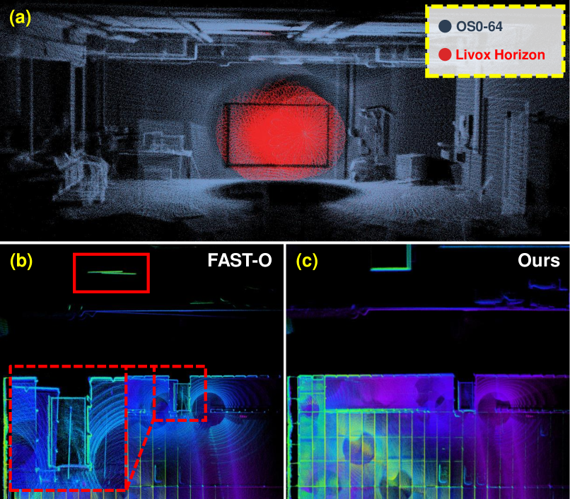
Figure 4: (a) Accumulated scans from LAB. Compared to Ouster (gray), Livox (red) reveals very limited FOV and causes localization failure due to the lack of distinct features. (b-c) show the outputs of Fast-O and our method for the Parking dataset. As shown in the red box in (b), the map produced by Fast-O is misaligned when returning to the starting point, while our result in (c) is well aligned.

Meanwhile, unlike Fast-O, Fast-H is degenerated significantly due to the limited FOV of the LiDAR. The limited FOV of Livox is prone to encounter degenerate cases as depicted in Fig. 4(a). This FOV-induced limitation may yield a substantial tracking deviation even in the presence of a rich feature. In this perspective, Fast-O seems the best choice for most environments, but it is not optimal in all cases, particularly in the Parking. Since the ground truth of Parking is not provided, we examine the reconstructed map for qualitative evaluation as illustrated in Fig. 4(b). In the center of the Parking, a substantial number of points are not detected, causing a tracking error and drift in the map. On the other hand, our method can mitigate these issues by incorporating additional LiDAR as shown in Fig. 4(c), demonstrating the robustness of the multi-LiDAR system.

III-C UrbanNav Dataset

The UrbanNav Dataset consists of three spinning LiDARs with two mounted on both sides in an inclined configuration. This configuration maximizes the scanning area but with minimal overlap, and can detect objects at higher elevations that are invisible to the central LiDAR. However, since this dataset contains multiple dynamic objects at a higher driving speed, inter-LiDAR transformation encompasses significant variations due to temporal discrepancies from asynchrony.

TABLE III: UrbanNav Dataset Evaluation

		Fast-LIO2	M-LOAM	LOCUS 2.0	Ours
Mongok	ATEt	5.917	25.899	6.846	2.579
	ATEr	4.039	9.140	5.616	2.383
	RTEt	0.188	0.632	0.174	0.167
	RTEr	0.749	1.006	0.710	0.736
Whampoa	ATEt	7.066	31.482	18.124	4.236
	ATEr	7.066	8.286	9.404	4.600
	RTEt	0.390	0.710	0.339	0.207
	RTEr	1.034	1.213	1.238	1.033
TST	ATEt	8.783	53.682	33.292	2.342
	ATEr	6.640	21.584	13.367	5.085
	RTEt	0.494	2.177	0.841	0.351
	RTEr	1.264	1.355	1.748	1.261

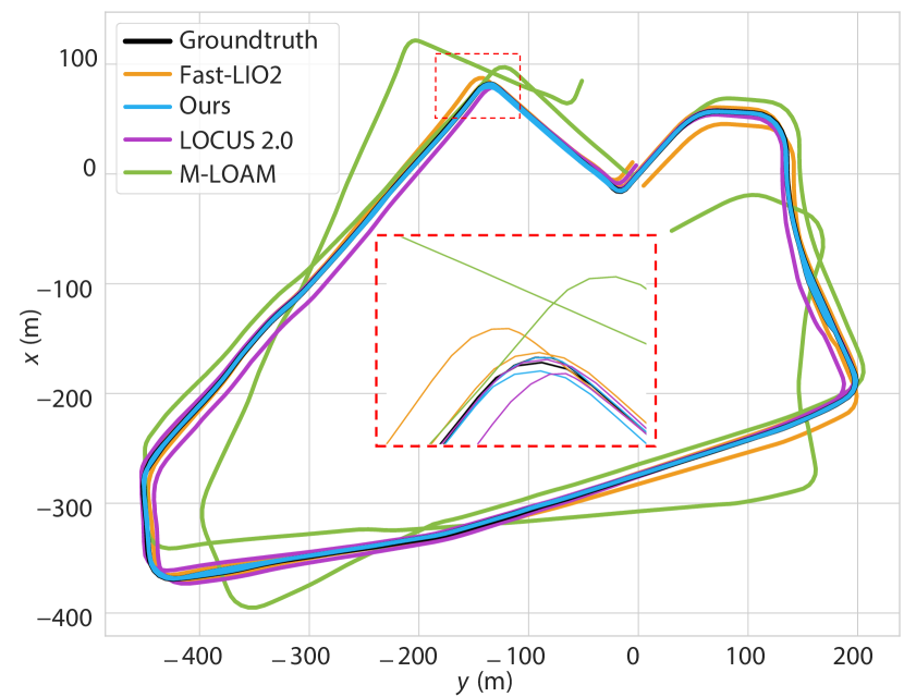
Figure 5: TST results. Our method (blue) demonstrates a highly close alignment with the ground truth (black).

As shown in Table III, our method outperforms all others. In the Mongok, most methods show minor errors due to the repeated traversal of a single loop. However, Whampoa exhibits more significant error in most algorithms as there is an underpass in the middle of the trajectory (Fig. 8(b)). Additionally, the higher vehicle speed in the TST—approximately twice that of the Mongok scenario—has exacerbated the error of the multi-LiDAR system due to the difficulties in merging pointclouds in asynchronous systems. Despite these challenges, the proposed method can effectively suppress significant errors by accurately estimating the relative transformation inter-LiDAR and allowing extensive scanning, which is impossible with a single LiDAR (Fig. 5).

III-D Our Own Dataset

TABLE IV: Private Dataset Evaluation

		Fast-LIO2	M-LOAM	LOCUS 2.0	Ours
City01	ATEt	9.970	33.907	23.998	6.538
	ATEr	4.575	8.792	5.521	3.491
	RTEt	0.292	0.955	0.609	0.266
	RTEr	0.898	1.020	0.895	0.874
City02	ATEt	35.308	72.382	58.211	6.707
	ATEr	7.473	4.683	4.722	3.522
	RTEt	0.608	3.665	1.531	0.565
	RTEr	1.179	1.104	1.167	1.084
City03	ATEt	6.951	33.801	21.753	5.470
	ATEr	4.194	6.657	4.773	3.522
	RTEt	0.996	1.310	1.159	0.565
	RTEr	1.088	1.070	1.089	1.084

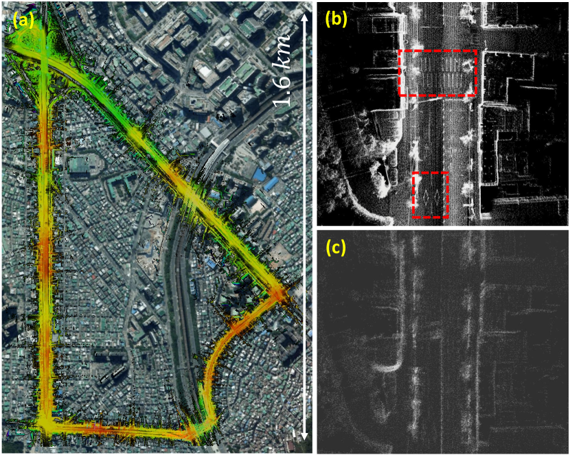
Figure 6: (a) The resulting map of City03. Points are color-coded by their height from low (red) to high (green). On the right, scans of stacks are presented from (b) our method and (c) LOCUS 2.0. Our method effectively compensates for temporal discrepancies, resulting in a low noise level even when markers on the street are present, as in the red box.

Our dataset, City01-03, presents a unique set of challenges, whereas our proposed method achieves superior performance in most cases, as presented in Table. IV. City01 includes many rotations and U-turns. After completing a U-turn, both M-LOAM and LOCUS 2.0 experienced localization failure when attempting to match the previously generated map. This failure is attributed to the lack of an initial estimation in LOCUS 2.0 and the inability to align the scans among LiDARs. As a result, the system resorts to constructing an additional map for localization.

City02 features a tunnel environment with a length of approximately $400\text{\,}\mathrm{m}$. In this sequence, failure to establish correspondences between points in the tunnel interrupts estimating forward motion yielding a significant error.

Lastly, City03 is over $4.3\text{\,}\mathrm{k}\mathrm{m}$ with numerous dynamic objects and no loops until the return to the start point with a large accumulated error. Among others, our method exhibits low error in City03, even in the absence of a loop in the middle of the trajectory. For example, the map is well-aligned after completing a single lap as presented in Fig. 6. Despite using asynchronous LiDAR, our method can generate clarified maps with reduced noise thanks to our temporal compensation and accurate odometry.

III-E The Effect of B-Spline and Uncertainty Propagation

(i) Module-wise comparison: Entire algorithm (FULL) consists of B-spline interpolation (CNT) and uncertainty propagation with localization weight (UNC). We test the baseline that exploits IMU discrete model and the same weight for all points (denoted as RAW). Additionally, we run a method that utilizes only one state covariance for uncertainty propagation, as in the case of M-LOAM (F-UNC). In this case, we exploit the last covariance of the scan as state covariance for point-wise uncertainty propagation. All of the methods are verified using ATE_t.

TABLE V: Component-wise comparison using ATE_t

	RAW	CNT	F-UNC	UNC	FULL
City01	7.345	7.280	7.001	6.831	6.538
City02	7.346	6.835	7.058	6.844	6.707
City03	6.043	5.969	6.547	5.837	5.470
Mongok	2.652	2.597	2.645	2.611	2.579
Whampoa	4.728	4.463	4.657	4.078	4.236
TST	2.721	2.143	2.773	2.752	2.324

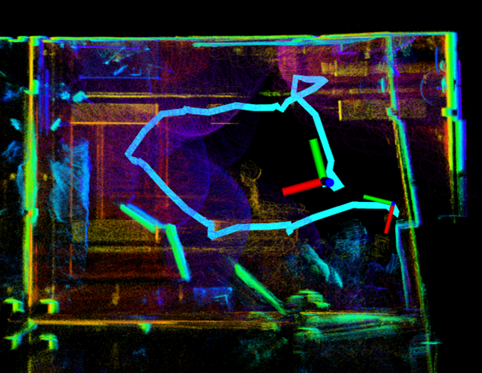
(a) The output of RAW

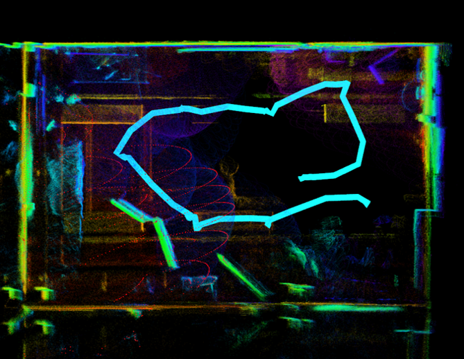
(b) The output of UNC

Figure 7: This map is generated using Livox Horizon after the successful initialization ($60\text{\,}\mathrm{s}\mathrm{e}\mathrm{c}$ from starting) in the LAB. (a) unsuccessful mapping in this degenerate environment. (b) consistent map by the proposed method overcoming the challenges environment.

Table. V presents the ATE_t for each test case. Both RAW and CNT address temporal discrepancies utilizing interpolation techniques; however, the CNT demonstrates slight improvement by using B-spline interpolation. This interpolation is particularly effective for datasets that exhibit highly curved trajectory. As expected, the ATE_t is reduced in the UrbanNav dataset, which has a higher IMU frequency ($400\text{\,}\mathrm{H}\mathrm{z}$) than the our own Dataset ($100\text{\,}\mathrm{H}\mathrm{z}$). This result demonstrates that temporal compensation and undistortion with B-spline interpolation are effective in both cases, regardless of the IMU frequency. The effect of point-wise uncertainty is the most critical, as can be seen from UNC, while F-UNC shows some level of error reduction but not as much as ours.

In City01-03, FULL yields the best results by effectively harnessing the benefits of both methods. However, the UrbanNav dataset shows varied results due to environmental factors. Stationary and low-speed segments lead to less pronounced effects of B-spline interpolation and point-wise uncertainty, resulting in similar performance in Mongok. In TST, the inclined LiDAR occasionally detects fewer points and becomes the primary LiDAR, leading to lower uncertainty compared to the front LiDAR. Consequently, the performance of UNC slightly declines compared to RAW, which subsequently impacts the results of FULL. Conversely, in Whampoa, increased environmental complexity allows for more effective point-wise uncertainty and localization weight, even when the primary LiDAR changed, resulting in significant performance increase in UNC. Although the competing effect between B-spline interpolation and point-wise uncertainty leads to lower performance in FULL compared to UNC, the error is significantly reduced compared to RAW. In conclusion, both proposed methods generally improves performance when uses individually or in combination.

(ii) Mapping capability: A qualitative comparison is given in Fig. 7 when we test RAW and UNC in LAB sequence. Because the small FOV is critically limited in this small indoor environment, this sequence is tricky to localize when equipped only with Livox Horizon. Unlike RAW that fails in consistent mapping, UNC localizes successfully in this confined space. As evidenced by the results in Table. V and Fig. 7, we can infer that the uncertainty model plays a leading factor in the enhancement of performance in our method.

(iii) Localization weights: In Fig. 8, we depict partial maps of the City02 and Whampoa. The narrow nature of these environments can cause a correspondence error, leading to the influence of prior residuals being stronger than measurement residuals. As can be seen from the Fig. 8(a) and (b), localization weight is significantly reduced only at the degenerate surroundings. This reduction is expected and demonstrates the effectiveness of our localization weight in these challenging environments.

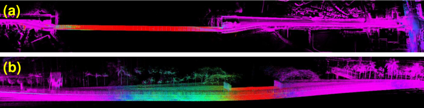
Figure 8: Partial maps of (a) City02 and (b) Whampoa with points color-coded by their localization weight from low (red) to high (purple). For both maps, a noticeable decrease in localization weight (red) only in the tunnel region. (b) the weight decrease is slighter than (a) because the upper part of the underpass is open and being scanned by inclined LiDAR.

III-F The Effect of the Number of LiDAR

To assess the real-time performance, we measure and analyze the average processing time per scan for each module, as in Fig. 9 and Table. VI.

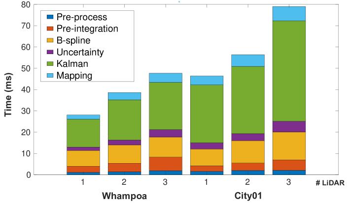
Figure 9: Computation times with respect to the number of LiDARs. Pre-process is the computation time for reformatting the pointcloud. Pre-integration involves integrating IMU measurements and undistorting the point. B-spline is utilized during undistortion and is separately listed from pre-integration. Uncertainty includes time for calculating the point-wise uncertainty and localization weight.

TABLE VI: Time analysis according to the number of LiDAR [ms]. The numbering follows the description in Table. I.

	Whampoa			City01
LiDAR #	1	2	3	1	2	3
Point (Down.) #	4045	5647	6784	8554	10172	12244
LiDAR	HDL-32E	+VLP-16	+LS-C16	OS2-128	+Avia	+Tele
Preprocess	1.1	1.4	1.9	1.6	2.0	2.1
Pre-integration	2.9	4	6.4	2.6	3.5	4.9
B-Spline	7.4	8.6	9.4	7.9	10.5	13.1
Uncertainty	1.6	2.3	3.5	2.9	3.3	5
Kalman Filter	13.1	18.9	22.2	27.2	31.6	47.2
Mapping	2.0	3.4	4.3	4.2	5.5	6.7
Total	28.1	38.6	47.7	46.4	56.4	79

*Specification: Intel i7 CPU@2.50Ghz and 48GB RAM

(i) Time: We analyze the time consumption for Whampoa and City01, which have the most extensive distance among the UrbanNav and our datasets. During all experiments, downsampling with $0.4$m resolution was implemented. Table. VI exhibits the number of points obtained following this operation. As can be seen, our method is light-weight and fully supports real-time performance even for a multi-LiDAR system. One of the modules in our method, uncertainty propagation, can be completed within a maximum of $5\text{\,}\mathrm{m}\mathrm{s}$, even though it significantly improves performance. In contrast, the B-spline interpolation takes longer because undistortion is done without downsampling. However, even in City01 with two Livox and an Ouster LiDAR, our method spends $79\text{\,}\mathrm{m}\mathrm{s}$ fully supporting $10\text{\,}\mathrm{H}\mathrm{z}$). Further improvement is possible by performing downsampling before the undistortion if needed.

(ii) Accuracy: The impact of the number of LiDAR on accuracy is further evaluated using three datasets: TST, Whampoa, and City03. For this test, we compare the results with RAW in City03. The errors decrease as the number of LiDAR increases, and the error range tends to decrease when checking the interquartile range and standard deviation in Fig. 10.

Interestingly, a significant error reduction is observed when the number increases from one to two, while a minor reduction is observed when the number increases from two to three (Fig. 10(a)). We speculate this is because an increment to two LiDARs provides sufficient constraints. Furthermore, as can be seen in the table in Fig. 10(b), it could be a fallacy to posit more LiDARs necessarily improve the performance. However, in City03, adding the second (Livox) and the third (Ouster) LiDARs could not effectively reduce the error because of the narrow FOV and wide overlap of the two LiDAR. Using two LiDARs with FULL outperforms using three LiDARs with RAW. This finding highlights the need for careful consideration of LiDAR placement in a multi-LiDAR system. Simply merging the pointcloud in the overlapping area may not necessarily lead to significant improvements in performance. Leveraging B-spline interpolation to locate points accurately and assign the uncertainty, FULL with three LiDARs gives the best performance.

IV conclusion

In this paper, we proposed a framework for asynchronous multiple LiDAR-inertial systems. The proposed framework utilizes B-spline interpolation in conjunction with an IMU discrete model to mitigate the temporal discrepancy among multiple LiDARs. To mitigate the accumulation of ambiguity during frame changes, a common issue in temporal compensation methods, we proposed a method for propagating point-wise uncertainty based on IMU acquisition time and point distance from sensors. Additionally, we incorporated a localization weight to improve performance in challenging environments. Our method was validated through extensive experimentation on both public datasets and our dataset and achieved real-time performance while surpassing the state-of-the-art in terms of accuracy and robustness.

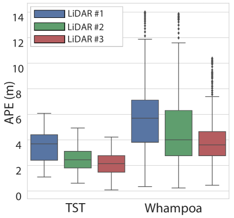
(a) ATE_t in the TST and Whampoa

No.	Median ATEt
1 (RAW)	5.76
1 (FULL)	5.65
2 (RAW)	5.27
2 (FULL)	5.08
3 (RAW)	5.22
3 (FULL)	4.73

(b) City03

Figure 10: 10(a) an evaluation about three cases for two datasets. From left, the median values of ATE_t and standard deviations are: (3.69, 1.22), (2.44, 0.96), (2.14, 0.98), (5.69, 2.53), (4.01, 2.69) and (3.58, 1.93). 10(b) shows the median ATE_t in City03 as a function of the number of LiDARs for the FULL and RAW.

References

- Jiao et al. [2021] J. Jiao, H. Ye, Y. Zhu, and M. Liu, “Robust odometry and mapping for multi-lidar systems with online extrinsic calibration,” IEEE Trans. Robot., vol. 38, no. 1, pp. 351–371, 2021.
- Helmberger et al. [2022] M. Helmberger, K. Morin, B. Berner, N. Kumar, G. Cioffi, and D. Scaramuzza, “The hilti slam challenge dataset,” IEEE Robot. and Automat. Lett., vol. 7, no. 3, pp. 7518–7525, 2022.
- Hsu et al. [2021] L. Hsu, N. Kubo, W. Wen, W. Chen, Z. Liu, T. Suzuki, and J. Meguro, “Urbannav: An open-sourced multisensory dataset for benchmarking positioning algorithms designed for urban areas,” in ION GNSS+, 2021, pp. 226–256.
- Nguyen et al. [2022] T.-M. Nguyen, S. Yuan, M. Cao, Y. Lyu, T. H. Nguyen, and L. Xie, “Ntu viral: A visual-inertial-ranging-lidar dataset, from an aerial vehicle viewpoint,” Intl. J. of Robot. Research, vol. 41, no. 3, pp. 270–280, 2022.
- Reinke et al. [2022] A. Reinke, M. Palieri, B. Morrell, Y. Chang, K. Ebadi, L. Carlone, and A. Agha-Mohammadi, “Locus 2.0: Robust and computationally efficient lidar odometry for real-time 3d mapping,” IEEE Robot. and Automat. Lett., vol. 7, no. 4, pp. 9043–9050, 2022.
- Palieri et al. [2020] M. Palieri, B. Morrell, A. Thakur, K. Ebadi, J. Nash, A. Chatterjee, C. Kanellakis, L. Carlone, C. Guaragnella, and A. Agha-Mohammadi, “Locus: A multi-sensor lidar-centric solution for high-precision odometry and 3d mapping in real-time,” IEEE Robot. and Automat. Lett., vol. 6, no. 2, pp. 421–428, 2020.
- Lin et al. [2020] J. Lin, X. Liu, and F. Zhang, “A decentralized framework for simultaneous calibration, localization and mapping with multiple lidars,” in Proc. IEEE/RSJ Intl. Conf. on Intell. Robots and Sys., 2020, pp. 4870–4877.
- Nguyen et al. [2021] T. Nguyen, S. Yuan, M. Cao, L. Yang, T. Nguyen, and L. Xie, “Miliom: Tightly coupled multi-input lidar-inertia odometry and mapping,” IEEE Robot. and Automat. Lett., vol. 6, no. 3, pp. 5573–5580, 2021.
- Wang et al. [2022] Y. Wang, W. Song, Y. Lou, F. Huang, Z. Tu, and S. Zhang, “Simultaneous localization of rail vehicles and mapping of environment with multiple lidars,” IEEE Robot. and Automat. Lett., vol. 7, no. 3, pp. 8186–8193, 2022.
- Lv et al. [2021] J. Lv, K. Hu, J. Xu, Y. Liu, X. Ma, and X. Zuo, “Clins: Continuous-time trajectory estimation for lidar-inertial system,” in Proc. IEEE/RSJ Intl. Conf. on Intell. Robots and Sys., 2021, pp. 6657–6663.
- Mueggler et al. [2018] E. Mueggler, G. Gallego, H. Rebecq, and D. Scaramuzza, “Continuous-time visual-inertial odometry for event cameras,” IEEE Trans. Robot., vol. 34, no. 6, pp. 1425–1440, 2018.
- Feng et al. [2018] D. Feng, L. Rosenbaum, and K. Dietmayer, “Towards safe autonomous driving: Capture uncertainty in the deep neural network for lidar 3d vehicle detection,” in Proc. IEEE Intell. Transport. Sys. Conf. IEEE, 2018, pp. 3266–3273.
- Meyer and Thakurdesai [2020] G. P. Meyer and N. Thakurdesai, “Learning an uncertainty-aware object detector for autonomous driving,” in 2020 IEEE/RSJ International Conference on Intelligent Robots and Systems (IROS). IEEE, 2020, pp. 10 521–10 527.
- Jung et al. [2021] Y. Jung, M. Jeon, C. Kim, S. Seo, and S. Kim, “Uncertainty-aware fast curb detection using convolutional networks in point clouds,” in Proc. IEEE Intl. Conf. on Robot. and Automat., 2021, pp. 12 882–12 888.
- Jiao et al. [2020] J. Jiao, P. Yun, L. Tai, and M. Liu, “Mlod: Awareness of extrinsic perturbation in multi-lidar 3d object detection for autonomous driving,” in Proc. IEEE/RSJ Intl. Conf. on Intell. Robots and Sys., 2020, pp. 10 556–10 563.
- Barfoot and Furgale [2014] T. Barfoot and P. Furgale, “Associating uncertainty with three-dimensional poses for use in estimation problems,” IEEE Trans. Robot., vol. 30, no. 3, pp. 679–693, 2014.
- Jiang and Shen [2022] B. Jiang and S. Shen, “A lidar-inertial odometry with principled uncertainty modeling,” in Proc. IEEE/RSJ Intl. Conf. on Intell. Robots and Sys., 2022, pp. 13 292–13 299.
- Xu et al. [2022] W. Xu, Y. Cai, D. He, J. Lin, and F. Zhang, “Fast-lio2: Fast direct lidar-inertial odometry,” IEEE Trans. Robot., vol. 38, no. 4, pp. 2053–2073, 2022.
- Xu and Zhang [2021] W. Xu and F. Zhang, “Fast-lio: A fast, robust lidar-inertial odometry package by tightly-coupled iterated kalman filter,” IEEE Robot. and Automat. Lett., vol. 6, no. 2, pp. 3317–3324, 2021.
- Grupp [2017] M. Grupp, “Evo: Python package for the evaluation of odometry and slam.” https://github.com/MichaelGrupp/evo, 2017.