On the Generalization and Approximation Capacities of Neural Controlled Differential Equations

Abstract

Neural Controlled Differential Equations (NCDEs) are a state-of-the-art tool for supervised learning with irregularly sampled time series (Kidger et al., 2020). However, no theoretical analysis of their performance has been provided yet, and it remains unclear in particular how the irregularity of the time series affects their predictions. By merging the rich theory of controlled differential equations (CDE) and Lipschitz-based measures of the complexity of deep neural nets, we take a first step towards the theoretical understanding of NCDE. Our first result is a generalization bound for this class of predictors that depends on the regularity of the time series data. In a second time, we leverage the continuity of the flow of CDEs to provide a detailed analysis of both the sampling-induced bias and the approximation bias. Regarding this last result, we show how classical approximation results on neural nets may transfer to NCDEs. Our theoretical results are validated through a series of experiments.

1 Introduction

Time series are ubiquitous in many domains such as finance, agriculture, economics and healthcare. A common set of tasks consists in predicting an outcome $y\in\mathcal{Y}$, such as a scalar or a label, from a time-evolving set of features. This problem has been addressed with a great variety of methods, ranging from Vector Auto-Regressive (VAR) models (Hamilton, 2020) and Gaussian processes (Roberts et al., 2013), to deep models such as Recurrent Neural Networks (RNN, Elman, 1991) and Long-Short-Term-Memory Networks (LSTM, Hochreiter & Schmidhuber, 1996).

Irregular Time Series.

In real-world scenarios, time series are often irregularly sampled (when data collection is difficult or expensive for instance). Mathematically, for a time series $\mathbf{x}=(\mathbf{x}_{t_{0}},\dots,\mathbf{x}_{t_{K}})\in\mathbb{R}^{d\times(K+1)}$, this means that $\Delta_{j}:=t_{j}-t_{j-1}$ may vary with $j=1,\dots,K$. We are interested in understanding the effect of coarseness of sampling on the learning performance. Intuitively, coarser sampling makes learning harder: bigger gaps between sampling times increase the probability of missing important events - say, a spike in the data - that help predict the outcome. Formally, it is natural to consider that the time series $\mathbf{x}$ is a degraded version - through subsampling - of an unobserved underlying path $x=(x_{t})_{t\in[0,1]}$ which, in turn, determines the outcome $y\in\mathcal{Y}\subset\mathbb{R}$. On a high level perspective, we have that $y=F(x)+\varepsilon$, where $F$ is an operator that maps the space of paths $\{x:[0,1]\to\mathbb{R}^{d}\}$ to $\mathcal{Y}$, and $\varepsilon$ is a noise term. For instance, in healthcare, the value of a vital of interest of a patient is determined by the continuous and unobserved trajectory of her biomarkers, rather than by the discrete measurements made by a physician.

Models for Irregular Time Series.

While many models and approaches have been proposed for learning from irregular time series (see Section 2), a quite fruitful point of view is to view the irregular data and the outcome as being linked through a dynamical system. In this article, we focus on Neural Controlled Differential Equations (NCDE), which take this point of view. NCDEs learn a time-dependant vector field, continuously evolving with the streamed data, that steers a latent state. The terminal value of this latent state is then eventually used for prediction - as one would for instance do with RNNs.

Our setup.

We restrict our attention to a supervised learning setup in which sampling times are arbitrarily spaced. Consider a sample $\{(y^{i},\mathbf{x}^{D,i})\}$, where $y^{i}\in\mathcal{Y}$ is the label of a time series $\mathbf{x}^{D,i}\in\mathbb{R}^{d\times(K+1)}$ discretized on an arbitrary grid $D=\{t_{0},\dots,t_{K}\}$. We will always require that this sampling grid is constant across individuals, and assume that $t_{0}=0$ and $t_{K}=1$. The first restriction can be easily relaxed following Bleistein et al. (2023), at the price of heavier notations. We consider a predictor $\hat{f}^{D}$ obtained by empirical risk minimization (ERM) on this sample.

While NCDE have been proven to yield excellent performance on supervised learning tasks (Kidger et al., 2020; Morrill et al., 2021a; Qian et al., 2021; Seedat et al., 2022; Norcliffe et al., 2023), little is known about their theoretical properties. This article aims at filling this gap by addressing three theoretical questions.

1. How do NCDE generalize i.e. how well does $\hat{f}^{D}$ perform on unseen data drawn from the same distribution that the training data ?

2. How well can NCDE approximate general controlled dynamical systems ?

3. How does the irregular sampling affect generalization and approximation ? Put otherwise, how does the predictor $\hat{f}^{D}$ compare to a theoretical predictor $\hat{f}$ obtained by ERM on the unseen streamed data ?

Our work is, to our knowledge, the first to address these critical questions. The last point is particularly crucial, since it determines how temporal sampling affects prediction performance. This is a central question both from a theoretical perspective and for practitioners, since it could, for instance, justify increasing sampling frequencies of ICU patients (Johnson et al., 2020).

Contribution.

Our contribution is threefold. First, we use a Lipschitz-based argument to obtain a sampling-dependant generalization bound for NCDE. To the best of our knowledge, this is the first bound of this kind. In a second time, we build on a CDE-based well-specified model to obtain a precise decomposition of the approximation and sampling bias. With these techniques at hand, we are able to precisely assess how approximation and generalization are affected by irregular sampling. Our theoretical results are illustrated by experiments on synthetic data.

Overview.

Section 2 covers related works. Section 3 details our setup and assumptions. In Section 4, we state our first result which is a generalization bound for NCDE. Section 5 gives an upper bound on the total risk, which is our second major result. Finally, we provide numerical illustrations in Section 6.

2 Related works

Hybridization of deep learning and differential equations.

The idea of combining differential systems and deep learning algorithms has been around for many years (Rico-Martinez et al., 1992; 1994). The recent work of Chen et al. (2018) has revived this idea by proposing a model which learns a representation of $x\in\mathbb{R}^{d}$ by using it to set the initial condition $z_{0}=\varphi^{\star}_{\xi}(x)$ of the ordinary differential equation (ODE)

$$dz_{t}=\mathbf{G}_{\psi}(z_{t})dt,$$

where $\mathbf{G}_{\psi}$ and $\varphi^{\star}_{\xi}$ are neural networks. The terminal value $z_{1}$ of this ODE is then used as input of any classical machine learning algorithm. Numeral contributions have build upon this idea and studied the connection between deep learning and differential equations in recent years (Dupont et al., 2019; Chen et al., 2019b; 2020; Finlay et al., 2020). Massaroli et al. (2020) and Kidger (2022) offer comprehensive introductions to this topic.

Learning with irregular time series.

Numerous models have been proposed to handle time-dependant irregular data. Che et al. (2018) introduce a modified Gated Recurrent Unit (GRU) with learnt exponential decay of the hidden state between sampling times. Other models hybridizing classical deep learning architectures and ODE include GRU-ODE (De Brouwer et al., 2019) and RNN-ODE (Rubanova et al., 2019).

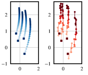
Figure 1: 2D latent state of a CDE driven by the smooth path $x_{t}=(t,t)$, i.e. a regular ResNet, on the left and a CDE driven by a Brownian motion with drift $x_{t}=(t+W^{(1)}_{t},t+W^{(2)}_{t})$ on the right. The square markers indicate the initial values of the latent states. The color gradient indicates evolution through time.

Neural Controlled Differential Equations have been introduced through two distinct frameworks, namely Neural Rough Differential Equations (Morrill et al., 2021b) and NCDEs (Kidger et al., 2020). In this article, we focus on the latter which extends neural ODEs to sequential data by first interpolating a time series $\mathbf{x}^{D}$ with cubic splines. The first value of the time series and the interpolated path $\tilde{\mathbf{x}}$ are then used as initial condition and driving signal of the CDE

$$dz_{t}=\mathbf{G}_{\psi}(z_{t})d\tilde{\mathbf{x}}_{t}$$

or equivalently

$$z_{t}=\varphi^{\star}_{\xi}(x_{0})+\int_{0}^{t}\mathbf{G}_{\psi}(z_{s})d\tilde{\mathbf{x}}_{s}.$$

We refer to Appendix A.1 for a formal definition. As for neural ODEs, the terminal value of this NCDE is then used for classification or regression. Other methods for learning from irregular time series include Gaussian Processes (Li & Marlin, 2016) and the signature transform (Chevyrev & Kormilitzin, 2016; Fermanian, 2021; Bleistein et al., 2023).

Generalization Bounds.

The generalization capacities of recurrent networks have been studied since the end of the 1990s, mainly through bounding their VC dimension (Dasgupta & Sontag, 1995; Koiran & Sontag, 1998). Bartlett et al. (2017) sparked a line of research connecting the Lipschitz constant of neural networks to their generalization capacities. Chen et al. (2019a) leverage this technique to derive generalization bounds for RNN, LSTM and GRU. Fermanian et al. (2021) also obtain generalization bounds for RNN and a particular class of NCDE. However, they crucially impose restrictive regularity conditions which then allow for linearization of the NCDE in the signature space. Generalization bounds are then derived using kernel learning theory. Hanson & Raginsky (2022) consider an encoder-decoder setup involving excess risk bounds on neural ODEs. Closest to our work is the recent work of Marion (2023), which leverages similar tools to study the generalization capacities of a particular class of neural ODE and deep ResNets. Our work is the first one analysing NCDEs. Recent related work is summarized in Table 1, and a detailed comparison between ResNets and NCDEs is given in Appendix F.1 - see also Figure 1 for an illustration.

Approximation Bounds.

The approximation capacities of neural ODEs have notably been studied by Zhang et al. (2020) and Ruiz-Balet & Zuazua (2023). In their seminal work on NCDE, Kidger et al. (2020) show that their are dense in the space of continuous functions acting on time series. In contrast to this work, we provide a precise decomposition of the approximation error when the outcome is generated by an unknown controlled dynamical system.

Article	Data	Model	Proof Technique	Approximation Error
Bartlett et al. (2017)	Static	$H(x)=W_{L}\circ\sigma\circ W_{L-1}\circ\dots\circ W_{1}(x)$	Lipschitz continuity	✗
		(MLP)	w.r.t. to $(W_{i})_{i=1}^{L}$
Chen et al. (2019a)	Sequential	$H_{t+1}=\sigma\big{(}AH_{t}+BX_{t}+C\big{)}$ (RNN)	Bartlett et al. (2017)	✗
Fermanian et al. (2021)	Sequential	$H_{t+1}=H_{t}+\frac{1}{L}\sigma\big{(}AH_{t}+BX_{t}+C\big{)}$	Kernel-based	✗
		(Residual RNN)	generalization bounds
Hanson & Raginsky (2022)	Static	$x\approx e^{a_{m}(x)f_{m}}\circ\dots\circ e^{a_{1}(x)f_{1}}\xi$	Control theory bound	NA
		(ODE-Autoencoder)
Marion (2023)	Static	$dH_{t}=W_{t}\sigma(H_{t})dt$ (Neural ODE)	Bartlett et al. (2017)	✗
		$H_{t+1}=H_{t}+\frac{1}{L}W_{t+1}\sigma(H_{t})$ (ResNet)
This article	Sequential	$dH_{t}=\mathbf{G}_{\theta}(H_{t})dX_{t}$ (Neural CDE)	Bartlett et al. (2017)	✓
		$H_{t+1}=H_{t}+\mathbf{G}_{\theta}(H_{t})\Delta X_{t+1}$	+ Continuity of the flow
		(Controlled ResNet)

Table 1: Summary of recent related works on generalization bounds. We do not include prior results leveraging VC dimensions. We refer to the cited work for precise definitions.

3 Learning with Controlled Differential Equations

3.1 Neural Controlled Differential Equations

We first define Neural Controlled Differential Equations driven by a very general class of paths.

Definition 3.1.

Let $x:=(x_{t})_{t\in[0,1]}\in\mathbb{R}^{d}$ be a continuous path and let $\mathbf{G}_{\psi}:\mathbb{R}^{p}\to\mathbb{R}^{p\times d}$ be a neural vector field parameterized by $\psi$. Consider the solution $z:=(z_{t})_{t\in[0,1]}\in\mathbb{R}^{p}$ of the controlled differential equation

$$dz_{t}=\mathbf{G}_{\psi}(z_{t})dx_{t},$$

with initial condition $z_{0}=\varphi_{\xi}(x_{0})$, where $\varphi_{\xi}:\mathbb{R}^{d}\to\mathbb{R}^{p}$ is a neural network parameterized by $\xi$. We call $z$ the latent space trajectory and

$$\Phi^{\top}z_{1}=:f_{\theta}(x)\in\mathbb{R},$$

for $\Phi\in\mathbb{R}^{p}$, the prediction of the NCDE with parameters $\theta=(\Phi,\psi,\xi)$.

The Picard-Lindelöf Theorem, recalled in Appendix A.2), ensures that the solution of this NCDE is well defined if the path $(x_{t})_{t\in[0,1]}$ is of bounded variation. We make the following hypothesis on $x$ in line with this theorem.

Assumption 1.

The path $(x_{t})_{t\in[0,1]}$ is $L_{x}$-Lipschitz continuous, that is $\left\lVert x_{t}-x_{s}\right\rVert\leq L_{x}\lvert t-s\rvert$ for all $s,t\in[0,1]$.

Assumption 1 indeed implies that $x$ has finite bounded variation, or put otherwise for all $t\in[0,1]$,

$$\left\lVert x\right\rVert_{\textnormal{1-var},[0,t]}:=\sup\limits_{D}\sum\left\lVert x_{t_{i+1}}-x_{t_{i}}\right\rVert\leq L_{x}t\leq L_{x},$$

where the supremum is taken on all finite discretizations $D=\{0=t_{0}<t_{1}<\dots<t_{N}=t\}$ of $[0,t]$, for $N\in\mathbb{N}^{*}$. Turning to our data $\{(\mathbf{x}^{D,i}),y_{i}\}$, we make two assumptions.

Assumption 2.

For every individual $i=1,\dots,n$, the time series $\mathbf{x}^{D,i}$ is a discretization of a path $(x^{i}_{t})_{t\in[0,1]}$ satisfying Assumption 1, i.e. $\mathbf{x}^{D,i}_{t_{k}}=x^{i}_{t_{k}}$ for all $k=0,\dots,K$.

Assumption 3.

There exists a constant $B_{x}>0$ such that for every individual $i=1,\dots,n$, $\left\lVert x^{i}_{0}\right\rVert\leq B_{x}$.

Neural vector fields.

The vector field $\mathbf{G}_{\psi}$ can be any common neural network, since most architectures are Lipschitz continuous with respect to their input (Virmaux & Scaman, 2018). This ensures that the solution of the NCDE is well defined. We restrict our attention to deep feed-forward neural vector fields with $q$ hidden layers of the form

$$\mathbf{G}_{\psi}(z)=\sigma\Big{(}\mathbf{A}_{q}\sigma\Big{(}\mathbf{A}_{q-1}\sigma\Big{(}\dots\sigma\Big{(}\mathbf{A}_{1}z+\mathbf{b}_{1}\Big{)}\Big{)}+\mathbf{b}_{q-1}\Big{)}+\mathbf{b}_{q}\Big{)},$$ (1)

with $L_{\sigma}$-Lipschitz activation function $\sigma:\mathbb{R}\to\mathbb{R}$ acting entry-wise that verifies $\sigma(0)=0$. Our framework can be extended to architectures with different activation functions: in this case, $L_{\sigma}$ will be defined as the maximal Lipschitz constant. Also note that the last activation function can be taken to be the identity. For every $h=1,\dots,q$, $\mathbf{A}_{h}:\mathbb{R}^{p_{h-1}}\to\mathbb{R}^{p_{h}}$ is a linear operator and $\mathbf{b}\in\mathbb{R}^{p_{h}}$ a bias term. Since the neural vector field $\mathbf{G}_{\psi}$ maps $\mathbb{R}^{p}$ to $\mathbb{R}^{p\times d}$, the dimensions of the first and last hidden layer must verify $p_{0}=p$ and $p_{q-1}=dp$. To alleviate notations and without loss of generality, we fix the size of hidden layers (but the last one) to be uniformly equal to $p$. Put otherwise, for every $h=1,\dots,q-1$, $\mathbf{A}_{h}\in\mathbb{R}^{p\times p}$ and $\mathbf{b}_{h}\in\mathbb{R}^{p}$, while $\mathbf{A}_{q}\in\mathbb{R}^{p\times dp}$ and $\mathbf{b}_{q}\in\mathbb{R}^{p\times d}$.

Following Kidger (2022), we restrict ourselves to initializations of the form

$$z_{0}=\varphi^{\star}_{\xi}(x_{0})=\sigma(\mathbf{U}x_{0}+v),$$ (2)

where $\mathbf{U}\in\mathbb{R}^{p\times d}$ and $v\in\mathbb{R}^{p}$. We use the notation $\text{NN}_{\mathbf{U},v}:u\mapsto\sigma\big{(}\mathbf{U}u+v\big{)}$ to refer to this initialization network. The activation function is assumed to be identical for the initialization layer and the neural vector field, but such an assumption can be relaxed. The learnable parameters of the model are therefore the linear readout $\Phi$, the hidden parameters $\psi=\Big{(}\mathbf{A}_{q},\dots,\mathbf{A}_{1},\mathbf{b}_{q},\dots,\mathbf{b}_{1}\Big{)}$, and the initialization weights $\xi=(\mathbf{U},v)$. We write $\theta=\big{(}\Phi,\psi,\xi\big{)}$ for the collection of these parameters.

Learning with time series.

To apply NCDEs to time series $\mathbf{x}^{D}$, one needs to embed $\mathbf{x}^{D}$ into the space of paths of bounded variation. This can be done through any reasonable embedding mapping

$$\rho:\mathbf{x}^{D}\in\big{(}\mathbb{R}^{d}\big{)}^{K+1}\mapsto(\tilde{\mathbf{x}}_{t})_{t\in[0,1]}$$

such as splines, polynomials or linear interpolation. In this work, we focus on the fill-forward embedding, which simply defines the value of $\tilde{\mathbf{x}}$ between two consecutive points of $D$ as the last observed value of $\mathbf{x}^{D}$.

Definition 3.2.

The fill-forward embedding of a time series $\mathbf{x}^{D}=(\mathbf{x}_{t_{0}},\dots,\mathbf{x}_{t_{K}})$ sampled on $D=\{0=t_{0}<\dots<t_{K}=1\}$ is the piecewise constant path $(\tilde{\mathbf{x}}_{t})_{t\in[0,1]}$ defined for every $t\in[t_{k},t_{k+1}[$ as $\tilde{\mathbf{x}}_{t}=\mathbf{x}^{D}_{t_{k}}$ for $k\in\{0,\dots,K-1\}$, and $\tilde{\mathbf{x}}_{1}=\mathbf{x}_{t_{K}}=x_{1}$.

Using this embedding in a NCDE with parameters $\theta=(\Phi,\psi,\xi)$ recovers a piecewise constant latent space trajectory $z^{D}:=(z^{D}_{t})_{t\in[0,1]}$ recursively defined for every $t\in[t_{k},t_{k+1}[$ by

$$z^{D}_{t}=z^{D}_{t_{k-1}}+\mathbf{G}_{\psi}(z_{t_{k-1}})(\mathbf{x}_{t_{k}}-\mathbf{x}_{t_{k-1}})$$ (3)

for $k=1,\dots,K-1$ and initialized as $z_{0}^{D}:=z_{0}=\sigma(\mathbf{U}x_{0}+v)$. Formally, the prediction $\Phi^{\top}z^{D}_{1}$ is equal to

$$\Phi^{\top}z^{D}_{1}=f_{\theta}\circ\rho_{\textnormal{ FF }}\big{(}\mathbf{x}^{D}\big{)},$$

where $\rho_{\textnormal{ FF }}$ is the fill-forward operator. To lighten notations, we simply write $\Phi^{\top}z^{D}_{1}=f_{\theta}(\mathbf{x}^{D})$. This recursive architecture has been studied with random neural vector fields by Cirone et al. (2023) under the name of homogenous controlled ResNet because of its resemblance with the popular weight-tied ResNet (He et al., 2015). We highlight that the latent continuous state $z$ is more informative about the outcome $y$ than its discretized version $z^{D}$. Indeed, it embeds the full trajectory of $x$ while $z^{D}$ embeds a version of $x$ degraded through sampling.

Restrictions on the parameter space.

In order to obtain generalization bounds, we must furthermore restrict the size of parameter space by requiring that the parameters $\theta$ lie in a bounded set $\Theta$. This means that there exist $B_{\Phi},B_{\mathbf{A}},B_{\mathbf{b}},B_{\mathbf{U}},B_{v}$ such that

$$\left\lVert\mathbf{A}_{h}\right\rVert\leq B_{\mathbf{A}},\left\lVert\mathbf{b}_{h}\right\rVert\leq B_{\mathbf{b}},\left\lVert\mathbf{U}\right\rVert\leq B_{\mathbf{U}},\left\lVert v\right\rVert\leq B_{v},\left\lVert\Phi\right\rVert\leq B_{\Phi}$$ (4)

for all $h=1,\dots,q$ and for all NCDEs considered, where $\left\lVert\cdot\right\rVert$ is the Frobenius norm. Such restrictions are classical for deriving generalization bounds (Bartlett et al., 2017; Bach, 2021; Fermanian et al., 2021). We call

$$\mathcal{F}_{\Theta}=\Big{\{}f_{\theta}:(x_{t})_{t\in[0,1]}\mapsto f_{\theta}(x)\in\mathbb{R}\,\,\text{ s.t. }\,\,\theta\in\Theta\Big{\}}$$

this class of predictors. We also write

$$\mathcal{F}^{D}_{\Theta}=\Big{\{}f_{\theta}:\mathbf{x}^{D}\in\mathbb{R}^{d\times\lvert D\rvert}\mapsto f_{\theta}(\mathbf{x}^{D})\in\mathbb{R}\,\,\text{ s.t. }\,\,\theta\in\Theta\Big{\}}$$

for the class of homogenous controlled ResNets. We now state an important lemma, which ensures that the outputs of NCDEs remain bounded. It is a direct consequence of Gronwall’s Lemma, recalled in Lemma A.4.

Lemma 3.3.

One has that $f_{\theta}(x)$ is uniformly upper bounded by

$$M_{\Theta}:=B_{\Phi}L_{\sigma}\exp\big{(}(B_{\mathbf{A}}L_{\sigma})^{q}L_{x}\big{)}\Big{(}B_{\mathbf{U}}B_{x}+B_{v}+\kappa_{\Theta}(\mathbf{0})L_{x}\Big{)}$$

and $f_{\theta}(\mathbf{x}^{D})$ is upper bounded by

$$M_{\Theta}^{D}:=B_{\Phi}L_{\sigma}\Big{(}1+\big{(}L_{\sigma}B_{\mathbf{A}}\big{)}^{q}L_{x}\lvert D\rvert\Big{)}^{K}\Big{(}B_{\mathbf{U}}B_{x}+B_{v}+\kappa_{\Theta}(\mathbf{0})L_{x}\Big{)},$$

where $\kappa_{\Theta}(\mathbf{0})=L_{\sigma}B_{\mathbf{b}}\frac{\big{(}L_{\sigma}B_{\mathbf{A}}\big{)}^{q}-1}{L_{\sigma}B_{\mathbf{A}}-1}$ is an upper bound of $\left\lVert\mathbf{G}_{\psi}(\mathbf{0})\right\rVert_{\textnormal{op}}=:\max\limits_{\left\lVert u\right\rVert=1}\left\lVert\mathbf{G}_{\psi}(0)u\right\rVert$.

Remark 3.4.

In practice, NCDEs are used with shallow neural vector fields, i.e. $q$ is typically chosen to be less than $3$ (Kidger et al., 2020).

Remark 3.5.

It is natural to wonder whether $M_{\Theta}^{D}\to M_{\Theta}$ as $\lvert D\rvert\to 0$. This is indeed true for well-behaved samplings, i.e. when adding more sampling points decreases the mesh size $\lvert D\rvert$ at sufficient speed. Indeed, if $K^{-1}=\mathcal{O}(\lvert D\rvert)$, one can use the fact that $(1+\alpha x^{-1})^{x}\to\exp(\alpha)$ as $x\to 0$ to see that $M_{\Theta}^{D}\to M_{\Theta}$.

3.2 The learning problem

We now detail our learning setup. We consider an i.i.d. sample $\{(y^{i},\mathbf{x}^{D,i})\}_{i=1}^{n}\sim y,x$ with given discretization $D$. For a given predictor $f_{\theta}\in\mathcal{F}_{\Theta}$, define

$$\mathcal{R}^{D}_{n}(f_{\theta})=\frac{1}{n}\sum\limits_{i=1}^{n}\ell(y^{i},f_{\theta}(\mathbf{x}^{D,i}))\quad\text{and }\quad\mathcal{R}^{D}(f_{\theta})=\mathbb{E}_{x,y}\Big{[}\ell(y,f_{\theta}(\mathbf{x}^{D}))\Big{]}$$

as the empirical risk and the expected risk on the discretized data. Similarly, define

$$\mathcal{R}_{n}(f_{\theta})=\frac{1}{n}\sum\limits_{i=1}^{n}\ell(y^{i},f_{\theta}(x^{i}))\quad\text{ and}\quad\mathcal{R}(f_{\theta})=\mathbb{E}_{x,y}\Big{[}\ell(y,f_{\theta}(x))\Big{]}$$

as the empirical risk and expected risk on the continuous data. We stress that $\mathcal{R}_{n}(f_{\theta})$ cannot be optimized, since we do not have access to the continuous data. Let $\hat{f}^{D}\in\operatorname*{arg\,min}\limits_{\theta\in\Theta}\mathcal{R}_{n}^{D}(f_{\theta})$ be an optimal predictor obtained by empirical risk minimization on the discretized data. In order to obtain generalization bounds, the following assumptions on the loss and the outcome are necessary (Mohri et al., 2018).

Assumption 4.

The outcome $y\in\mathbb{R}$ is bounded a.s.

Assumption 5.

The loss $\ell:\mathbb{R}\times\mathbb{R}\to\mathbb{R}_{+}$ is Lipschitz with respect to its second variable, that is there exists $L_{\ell}$ such that for all $u,u^{\prime}\in\mathcal{Y}$ and $y\in\mathcal{Y}$, $\lvert\ell(y,u)-\ell(y,u^{\prime})\rvert\leq L_{\ell}\lvert u-u^{\prime}\rvert$.

This hypothesis is satisfied for most classical losses, such as the the mean squared error, as long as the outcome and the predictions are bounded. This is true by Assumption 4 and Lemma 3.3. The loss function is thus bounded since it is continuous on a compact set, and we let $M_{\ell}$ be a bound on the loss function.

4 A Generalization Bound for NCDE

We now state our main theorem.

Theorem 4.1.

One has, with probability at least $1-\delta$, that the generalization error $\mathcal{R}^{D}(\hat{f}^{D})-\mathcal{R}_{n}(\hat{f}^{D})$ is upper bounded by

$$\frac{24M^{D}_{\Theta}L_{\ell}}{\sqrt{n}}\sqrt{2pU^{D}_{1}+(q-1)p(p+1)U^{D}_{2}+dp(2+p)U^{D}_{3}}+M_{\ell}\sqrt{\frac{\log 1/\delta}{2n}},$$

with $U^{D}_{1}:=\log\sqrt{n}C_{q}K^{D}_{1}$, $U^{D}_{2}:=\log\sqrt{np}C_{q}K^{D}_{2}$, and $U_{3}^{D}=\log\sqrt{ndp}C_{q}K^{D}_{2}$ $C_{q}:=(8q+12)$. $K^{D}_{1}$ and $K^{D}_{2}$ are two discretization and depth dependant constants given in the proof.

This result is similar to results obtained for instance by Bartlett et al. (2017), Chen et al. (2019b) and Marion (2023) for different models. Indeed, the generalization error is upper bounded by a noise induced term and a complexity term which grows with the square root of the model’s complexity measured by the number of hidden layers $q$ and the dimension $p$ of the hidden state. Remark that the constant $M^{D}_{\Theta}$ grows exponentially with $q$ if $B_{\mathbf{A}}L_{\sigma}>1$. This theorem is obtained by upper bounding the covering number of $\mathcal{F}^{D}_{\Theta}$ and the Rademacher complexity of NCDEs.

Proposition 4.2.

When using discretized inputs, the covering number $\mathcal{N}\big{(}\mathcal{F}_{\Theta},\eta;D\big{)}$ of $\mathcal{F}^{D}_{\Theta}$ is bounded from above by

$$\Bigg{(}1+\frac{C_{q}K^{D}_{1}}{2\eta}\sqrt{p}\Bigg{)}^{(q+1)p(1+p)}\Bigg{(}1+\frac{C_{q}K^{D}_{2}}{2\eta}(\sqrt{p}+\sqrt{d})\Bigg{)}^{2dp}\Bigg{(}1+\frac{C_{q}K^{D}_{1}}{2\eta}\sqrt{dp}\Bigg{)}^{dp^{2}}.$$

Furthermore, the empirical Rademacher complexity $\textnormal{Rad}(\mathcal{F}^{D}_{\Theta})$ associated to an i.i.d. sample of size $n$ discretized on $D$ is upper bounded by

$$\frac{4}{n}+\frac{24M^{D}_{\Theta}}{\sqrt{n}}\sqrt{(q+1)p(p+1)U^{D}_{1}+2dpU_{2}^{D}+dp^{2}U_{3}^{D}}.$$

When using continuous inputs, the constants appearing in the upper bound of $\textnormal{Rad}(\mathcal{F}_{\Theta})$ are discretization independent.

This result is obtained by showing that NCDE are Lipschitz with respect to their parameters, such that covering each parameter class yields a covering of the whole class of predictors. In combination with arguments borrowed from Chen et al. (2019a) and Bartlett et al. (2017), one may then upper bound the empirical Rademacher complexity by making use of the Dudley Integral.

5 A Bound on the Total Risk

5.1 A CDE-Based Well-Specified Model

In order to bound the approximation bias, we introduce a model that links the underlying path $x$ to the outcome $y$.

Assumption 6.

There exists a vector field $\mathbf{G}^{*}:\mathbb{R}^{p}\to\mathbb{R}^{p\times d}$, a function $\varphi^{\star}:\mathbb{R}^{d}\to\mathbb{R}^{p}$ and a vector $\Phi_{\star}\in\mathbb{R}^{p}$ that govern a latent state $(z^{\star}_{t})_{t\in[0,1]}$ through the CDE

$$dz^{\star}_{t}=\mathbf{G}^{\star}(z^{\star}_{t})dx_{t}$$ (5)

with initial value $z^{\star}_{0}=\varphi^{\star}(x_{0})$ such that the outcome $y$ is given by

$$y=\Phi_{\star}^{\top}z_{1}^{\star}+\varepsilon,$$

where $\varepsilon$ is a noise term bounded by $M_{\varepsilon}>0$.

Assumption 7.

The parameters of the well-specified model satisfy $\left\lVert\Phi_{\star}\right\rVert\leq B_{\Phi}$, $\varphi^{\star}\in C(\mathbb{R}^{d},\mathbb{R}^{p})$ and $\mathbf{G}^{\star}\in\text{Lip}(\mathbb{R}^{p},\mathbb{R}^{p\times d})$ with Lipschitz constant $L_{\mathbf{G}^{\star}}$.

Remark 5.1.

This is a very general model, which encompasses ODE-based models used for instance in biology or physics. Indeed, by setting $x_{t}=t$ for all $t$, one recovers a generic ODE. It also allows for the modelization of complex dynamical systems whose dynamics depend on external time-dependant data. For instance, Simeoni et al. (2004) model tumor growth kinetics as a CDE driven by a time series recording the intake of anticancer agents, which perturbs the dynamics of the growth of the tumor.

We call the map $\mathbf{f}^{\star}:x\mapsto\Phi_{\star}^{\top}z_{1}^{\star}$ the true predictor. Uniqueness and existence to equation 5 is given by the Picard-Lindelöf theorem stated in Appendix A.2. We have the following important lemma, which ensures that outcomes of the well-specified model are bounded. Its is analogous to Lemma 3.3.

Lemma 5.2.

Let $y$ be generated from the CDE (5) from a $L_{x}$-Lipschitz path $x$. Let $B_{\varphi}^{\star}:=\max\limits_{\left\lVert u\right\rVert\leq B_{x}}\left\lVert\varphi^{\star}(u)\right\rVert$. Then Assumption 4 holds, i.e. $y$ is bounded, and one has

$$\lvert y\rvert\leq B_{\Phi}\Big{(}B_{\varphi}^{\star}+\left\lVert\mathbf{G}^{\star}(0)\right\rVert_{\textnormal{op}}L_{x}\Big{)}\exp\big{(}L_{\mathbf{G}^{\star}}L_{x}\big{)}+M_{\varepsilon}.$$

5.2 Bounding the Total Risk

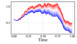
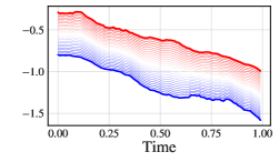
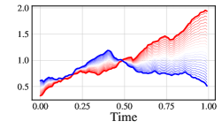
Figure 2: Left: in bold, we plot the solutions of two shallow $(q=1)$ NCDEs who only differ in their vector field $\mathbf{A}^{1}$ and $\mathbf{A}^{2}$. We then plot the solutions of the NCDEs with interpolated vector field $\delta\mathbf{A}^{1}+(1-\delta)\mathbf{A}^{2}$ for $\delta\in[0,1]$ in red-blue gradient. Center: we consider a given NCDE and interpolate linearly between two initial conditions $x^{1}_{0}$ and $x^{2}_{0}$. Right: we consider a given NCDE and drive it with the linear interpolation of two paths $(x^{1}_{t})_{t}$ and $(x^{2}_{t})_{t}$. In all three cases, the solutions evolve continuously as we interpolate between the models.

We first decompose the difference between the expected risk of $\hat{f}^{D}$ learnt from the sample $S$ and the expected risk of $\mathbf{f}^{*}$.

Lemma 5.3.

For all $f_{\theta}\in\mathcal{F}_{\theta}$, the total risk $\mathcal{R}^{D}(\hat{f}^{D})-\mathcal{R}(\mathbf{f}^{*})$ is almost surely bounded from above by

$$\sup\limits_{g\in\mathcal{F}^{D}_{\Theta}}\Big{[}\mathcal{R}^{D}(g)-\mathcal{R}_{n}^{D}(g)\Big{]}+\sup\limits_{g\in\mathcal{F}_{\Theta}}\Big{[}\mathcal{R}(g)-\mathcal{R}_{n}(g)\Big{]}+\underbrace{\mathcal{R}_{n}^{D}(f_{\theta})-\mathcal{R}_{n}(f_{\theta})}_{\textnormal{Discretization bias}}+\underbrace{\mathcal{R}(f_{\theta})-\mathcal{R}(\mathbf{f}^{*})}_{\textnormal{Approximation bias}}.$$

We let

$$\lvert D\rvert:=\max\limits_{j=1,\dots,K-1}\lvert t_{j+1}-t_{j}\rvert$$

be the greatest gap between two sampling times. Turning to the total risk, we get the following result by bounding every term of Lemma 5.3.

Theorem 5.4.

The total risk $\mathcal{R}^{D}(\hat{f}^{D})-\mathcal{R}(\mathbf{f}^{*})$ is bounded from above by

$$4\max\{\textnormal{Rad}(\mathcal{F}_{\Theta}),\textnormal{Rad}(\mathcal{F}^{D}_{\Theta})\}$$ (Worst-case bound)

$$+L_{\ell}B_{\Phi}L_{x}\Bigg{[}1+\big{(}L_{\sigma}B_{\mathbf{A}}\big{)}^{q}\Big{(}\big{(}L_{\sigma}B_{\mathbf{A}}\big{)}^{q}\frac{\min\{M^{D}_{\Theta},M_{\Theta}\}}{B_{\Phi}}+\kappa_{\Theta}(\mathbf{0})\Big{)}L_{x}\Bigg{]}\lvert D\rvert$$ (Discretization Bias)

$$+L_{\ell}B_{\Phi}\exp(L_{\mathbf{G}^{\star}}L_{x})\Big{[}L_{x}\min\limits_{\psi}\max\limits_{u\in\Omega}\left\lVert\mathbf{G}_{\psi}(u)-\mathbf{G}^{\star}(u)\right\rVert_{\textnormal{op}}+\min\limits_{\mathbf{U},v}\max\limits_{\left\lVert u\right\rVert\leq B_{x}}\left\lVert\varphi^{\star}(u)-\textnormal{NN}_{\mathbf{U},v}(u)\right\rVert\Big{]}.$$ (Approximation Bias)

Let us comment the three terms of the bound of Theorem 5.4. The first term is a common worst case bound when deriving generalization bounds and is bounded using Proposition 4.2. The second term corresponds to the discretization bias, and is directly proportional to $\lvert D\rvert$. It therefore vanishes at the same speed as $\lvert D\rvert$. For instance, if we consider the sequence $D_{K}$ of equidistant discretizations of $[0,1]$ with $K$ points, the discretization bias vanishes at linear speed. Finally, observe that the approximation bias writes as the sum of approximation errors on the vector fields and the initial condition, rather than a general approximation error on the true predictor $\mathbf{f}^{\star}$. The diameter of $\Omega$ is upper bounded in Proposition C.2.

Remark 5.5.

This decomposition of the approximation bias allows to leverage approximation results for feed forward neural networks to obtain precise bounds (see for instance Berner et al., 2021; Shen et al., 2021). This is left for future work.

Outline of the proof.

The proof schematically works in two times. We first bound the two sources of bias by leveraging the continuity of the flow of a CDE. Informally, this theorem states that the difference $\Delta(\text{terminal value})$ between the terminal value of two CDEs decomposes as

$$\Delta(\text{vector fields})+\Delta(\text{initial conditions})+\Delta(\text{driving paths}).$$

This neat decomposition allows us to bound the discretization bias since it depends on the terminal value of two CDEs whose driving paths differ. This property is illustrated in Figure 2. Combining these results with Theorem 4.1 gives Theorem 5.4.

6 Numerical Illustrations

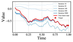
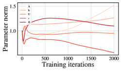
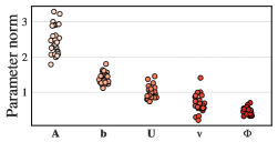
Figure 3: Left: Evolution of the prediction $(\Phi^{\top}z_{t})_{t}$ of a NCDE with shallow neural vector field at different moments of the training process ; the true process $(\Phi_{\star}^{\top}z^{\star}_{t})_{t}$ is shown in red. Center: Evolution of the parameter’s norms, normalized by their value at initialization, during training. Right: Parameters’ norm at the end of training, without normalization, over $25$ training instances of the same model. Training is performed with Adam (Kingma & Ba, 2014).

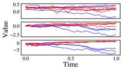
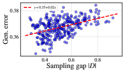
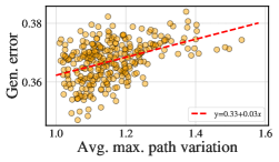
Figure 4: Left: latent state $(\Phi^{\top}z_{t})_{t}$ at initialization (top) and after $10$ (middle) resp. $100$ (bottom) training steps as the NCDE learns to separate rough (in red) from smooth (in blue) paths on a fine grid. The figure shows examples from the test set. Center: Generalization error $\lvert n^{-1}\sum\ell(\mathbf{x}^{D,i},y^{i})-\mathbb{E}_{\mathbf{x}^{D},y}\,\ell(\mathbf{x}^{D},y)\rvert$ vs. sampling gap. Right: Generalization error vs. average maximal path variation. We train $300$ NCDEs, with $\Phi$ and the initialization layer left untrained to isolate the effect of the discretization, with time series downsampled on $K=5$ points randomly chosen in $[0,1]$ for each run. Training is done with Adam with default parameters (Kingma & Ba, 2014).

Training Dynamics.

Our proofs rely on the restriction that all considered predictors, including $\hat{f}^{D}$ obtained by ERM, have parameters lying in a bounded set $\Theta$. To check whether this hypothesis is reasonable, we examine the evolution of the parameters’ norms during training. Figure 3 displays the evolution of the latent state of a shallow model ($q=1$) through training, along with the evolution of the normalized parameter norm, in a teacher-student i.e. well-specified setup. The trained NCDE achieves perfect interpolation of the outcome but also, more surprisingly, almost perfect interpolation of the unobserved latent state. We also observe little dispersion of the parameters’ norm over multiple training instances.

Effect of the Discretization.

Our bounds highlight the effect of the discretization gap $\lvert D\rvert$ on the generalization capacities of NCDEs. In our second experiment, presented in Figure 4, we consider a classification task in which a NCDE is trained to distinguish between rough ($H=0.4$) and smoother ($H=0.6$) discretized sample paths of a fractional Brownian Motion (fBM) with Hurst exponent $H$. We randomly downsample the paths, train the model and compute the generalization error in terms of binary cross entropy loss. We see a clear correlation between the generalization error and the sampling gap $\lvert D\rvert$. Since our bound involving $\lvert D\rvert$ relies on the inequality

$$\max_{k=1,\dots,K}\left\lVert\mathbf{x}^{D,i}_{t_{k+1}}-\mathbf{x}^{D,i}_{t_{k}}\right\rVert\leq\max_{k=1,\dots,K}L_{x}\lvert t_{k+1}-t_{k}\rvert\leq L_{x}\lvert D\rvert,$$

we also check for correlation with the average maximal path variation

$$n^{-1}\sum\limits_{i=1}^{n}\max_{k=0,\dots,K}\left\lVert\mathbf{x}^{D,i}_{t_{k+1}}-\mathbf{x}^{D,i}_{t_{k}}\right\rVert.$$

As predicted, this quantity also correlates with the generalization error. This is consistent with the findings of Marion (2023), who observe that the generalization error of ResNets scales with the Lipschitz constant of the weights (see Appendix F.1 for a detailed discussion). All experimental details are given in Appendix E.

7 Conclusion

We have answered three open theoretical questions on NCDE. First, we have provided a generalization bound for this class of models. In a second time, we have shown that under the hypothesis of CDE-based well-specified model, the approximation bias of NCDE decomposes into a sum of tractable biases. Most importantly, all our results are discretization-dependent and allow to precisely quantify the theoretical impact of the time series sampling on the model’s performance.

Acknowledgements.

We thank Pierre Marion and Adeline Fermanian for proofreading and providing insightful comments and remarks, and Cristopher Salvi for discussions on Controlled ResNets. LB conducted parts of this research while visiting MBZUAI’s Machine Learning Department (UAE).

The appendix is structured as follows. Appendix A gives preliminary results on CDEs and covering numbers. Appendix B.3 collects the proofs of the generalization bound. Appendix C details the proof of the bounds of the approximation and discretization biases and the bound on the total risk. Proofs of Appendix A are given in Appendix D for the sake of clarity. Appendix E gives all experimental details.

Appendix A Mathematical background

A.1 Riemann-Stieltjes integral

Lemma A.1.

Let $f:[0,1]\to\mathbb{R}^{p\times d}$ be a continuous function, and $g:[0,1]\to\mathbb{R}^{d}$ be of finite total variation. Then Riemann-Stieljes integral

$$\int_{0}^{t}f_{s}dg_{s}\in\mathbb{R}^{p},$$

where the product is understood in the sens of matrix-vector multiplication, is well-defined and finite for every $t\in[0,1]$.

We refer to Friz & Victoir (2010) for a thorough introduction to the Riemann-Stieltjes integral.

A.2 Picard-Lindelöf Theorem

Theorem A.2.

Let $x$ be a continuous path of bounded variation, and assume that $\mathbf{G}:\mathbb{R}^{p}\to\mathbb{R}^{p\times d}$ is Lipschitz continuous. Then the CDE

$$dz_{t}=\mathbf{G}(z_{t})dx_{t}$$

with initial condition $z_{0}=\varphi^{\star}(x_{0})$ has a unique solution.

A full proof can be found in Fermanian et al. (2021). Remark that since in our setting, NCDEs are Lipschitz since the neural vector fields we consider are Lipschitz (Virmaux & Scaman, 2018). This ensures that the solutions to NCDEs are well defined.

We also need the following variation, which ensures that the CDE driven by $\tilde{\mathbf{x}}$ is well-defined.

Lemma A.3.

Let $x$ be a piecewise constant and right-continuous path taking finite values in $\mathbb{R}^{d}$, with a finite number of discontinuities at $0<t_{1},\dots,t_{K}=1$, i.e.

$$\lim\limits_{t\to t^{+}_{i}}x_{t}=x_{t_{i}}$$

and

$$x_{t}=x_{t_{i}}$$

for all $t\in[t_{i},t_{i+1}[$, for all $i=1,\dots,K-1$. Assume that $\mathbf{G}:\mathbb{R}^{p}\to\mathbb{R}^{p\times d}$ is Lipschitz continuous. Then the CDE

$$dz_{t}=\mathbf{G}(z_{t})dx_{t}$$

with initial condition $z_{0}=\varphi^{\star}(x_{0})$ has a unique solution.

This result can be obtained by first remarking that since $x$ is piecewise constant, the solution to this CDE will also be piecewise constant, with discontinues at $0<t_{1}<\dots<t_{K}$: indeed, the variations of $x$ between two points of discontinuity being null, the variations of the solution will also be null between these two points. The solution can then be recursively obtained by seeing that for all $t\in[t_{i},t_{i+1}[$

$$z_{t}=z_{t_{i}}=z_{t_{i-1}}+\mathbf{G}(z_{t_{i-1}})(\mathbf{x}_{t_{i}}-\mathbf{x}_{t_{i-1}})$$

with $z_{t}=\varphi^{\star}(z_{0})$ for $t\in[t_{0},t_{1}[$, where $t_{0}=0$, and $z_{t_{K}}=y_{1}=y_{t_{K-1}}+\mathbf{G}(y_{t_{K-1}})(\mathbf{x}_{t_{K}}-\mathbf{x}_{t_{K-1}})$.

A.3 Gronwall’s Lemmas

Lemma A.4 (Gronwall’s Lemma for CDEs).

Let $x:[0,1]\to\mathbb{R}^{d}$ be a continuous path of bounded variations, and $\phi:[0,1]\to\mathbb{R}^{d}$ be a bounded measurable function. If

$$\phi(t)\leq K_{t}+L_{x}\int_{0}^{t}\phi(s)\left\lVert dx_{s}\right\rVert$$

for all $t\in[0,1]$, where $K_{t}$ is a time dependant constant, then

$$\phi(t)\leq K_{t}\exp\big{(}L_{x}\left\lVert x\right\rVert_{\textnormal{1-var},[0,t]}\big{)}$$

for all $t\geq 0$.

See Friz & Victoir (2010) for a proof. Remark that this Lemma does not require $\phi(\cdot)$ to be continuous. We also state a variant of the discrete Gronwall Lemma, which will allow us to obtain the bound for discrete inputs $\mathbf{x}^{D}$.

Lemma A.5 (Gronwall’s Lemma for sequences).

Let $(y_{k})_{k\geq 0},(b_{k})_{k\geq 0}$ and $(f_{k})_{k\geq 0}$ be positive sequences of real numbers such that

$$y_{n}\leq f_{n}+\sum\limits_{l=0}^{n-1}b_{l}y_{l}$$

for all $n\geq 0$. Then

$$y_{n}\leq f_{n}+\sum\limits_{l=0}^{n-1}f_{l}b_{l}\prod\limits_{j=l+1}^{n-1}(1+b_{j})$$

for all $n\geq 0$.

A proof can be found in Holte (2009) and Clark (1987). We finally need a variant of Gronwall’s Lemma for sequences.

Lemma A.6.

Let $(u_{k})_{k\geq 0}$ be a sequence such that for all $k\geq 1$,

$$u_{k}\leq a_{k}u_{k-1}+b_{k}$$

for $(a_{k})_{k\geq 1}$ and $(b_{k})_{k\geq 1}$ two positive sequences. Then for all $k\geq 1$, one has

$$u_{k}\leq\Big{(}\prod\limits_{j=1}^{k}a_{j}\Big{)}u_{0}+\sum\limits_{j=1}^{k}b_{j}\Big{(}\prod\limits_{i=j+1}^{k}a_{i}\Big{)}.$$ (6)

A.4 Dudley’s Entropy Integral

We recall the following Lemma from Bartlett et al. (2017).

Lemma A.7.

Let $\mathcal{H}$ be a class of real-valued functions taking values in $[-M,M]$, for $M>0$, and assume that $0\in\mathcal{H}$. Then the empirical Rademacher complexity associated to a sample of $n$ datapoints verifies

$$\textnormal{Rad}(\mathcal{H})\leq\inf\limits_{\eta>0}\Bigg{[}\frac{4\eta}{\sqrt{n}}+\frac{12}{n}\int_{\eta}^{2M\sqrt{n}}\sqrt{\log\mathcal{N}(\mathcal{H},s)}ds\Bigg{]}.$$ (7)

A.5 Covering numbers

First, we recall the definition of the covering number of a class of functions.

Definition A.8.

Let $\mathcal{H}=\{h:\mathcal{U}\subset\mathbb{R}^{e}\to\mathbb{R}^{f}\}$ be a class of functions. The covering number $\mathcal{N}\big{(}\mathcal{H},\eta\big{)}$ of $\mathcal{H}$ is the minimal cardinality of a subset $C\subset\mathcal{H}$ such that for all $h\in\mathcal{H}$, there exists $\hat{h}\in C$ such that

$$\sup\limits_{x\in\mathcal{U}}\left\lVert h(x)-\hat{h}(x)\right\rVert\leq\eta.$$

We state a Lemma from Chen et al. (2019a) bounding the covering number of sets of linear maps.

Lemma A.9.

Let $\mathcal{G}=\{A\in\mathbb{R}^{f\times e}\text{ s.t. }\left\lVert A\right\rVert\leq\lambda\}$ for a given $\lambda>0$. The covering number $\mathcal{N}(\mathcal{G},\eta)$ is upper bounded by

$$\Bigg{(}1+\frac{2\min(\sqrt{e},\sqrt{f})\lambda}{\eta}\Bigg{)}^{ef}.$$

We now proceed to prove our main results. Let us precisely detail the different steps of our proofs.

1. For the generalization bound, the first step consists in showing that NCDEs are Lipschitz with respect to their parameters, which we do in Theorem B.6. This leverages the continuity of the flow, since we aim at bounding the difference between two NCDEs with different parameters but identical driving paths.

2. Building on Chen et al. (2019a), we then obtain a covering number for NCDE.

3. We connect the covering number of $\mathcal{F}_{\Theta}$ and $\mathcal{F}^{D}_{\Theta}$ to its Rademacher complexity building on arguments made by Bartlett et al. (2017) in Proposition 4.2.

4. Once this last result is obtained, we can obtain the generalization bound by resorting to classical techniques (Mohri et al., 2018).

5. The bound of the discretization bias, stated in Proposition C.1, follows from the continuity of the flow given in Theorem B.5. Indeed, the discretization error depends on the difference between $z_{1}$ and $z_{1}^{D}$, which are solutions to identical CDE, but with different driving paths $x$ and embedded path $\tilde{\mathbf{x}}$.

6. The bound of the approximation bias is obtained in a similar fashion. Indeed, it directly depends on the difference between $z^{\star}_{1}$ and $z_{1}$. However, this time, only the initial condition and the vector fields are different, while the driving paths are identical.

7. The bound on the total risk is obtained by combining all the precedent elements and using a symmetrization argument to upper bound the two worst case bounds.

Appendix B Proof of the Generalization Bound

B.1 Lipschitz Continuity of Neural Vector fields

We first state a series of Lemmas on the Lipschitz continuity of neural vector fields. We first prove Lipschitz continuity with respect to their inputs.

Lemma B.1.

Let $\mathbf{G}_{\psi}$ be a neural vector field of depth $q\geq 1$ as defined in Equation  1. Then one has for all $z,w\in\mathbb{R}^{p}$

$$\left\lVert\mathbf{G}_{\psi}(z)-\mathbf{G}_{\psi}(w)\right\rVert\leq\Big{(}L_{\sigma}B_{\mathbf{A}}\Big{)}^{q}\left\lVert z-w\right\rVert$$ (8)

Our second Lemma shows that the operator norm of neural vector fields grows linearly with $z$.

Lemma B.2.

Let $\mathbf{G}_{\psi}:\mathbb{R}^{p}\to\mathbb{R}^{p\times d}$ be a neural vector field of depth $q$. For all $z\in\mathbb{R}^{p}$, one has

$$\left\lVert\mathbf{G}_{\psi}(z)\right\rVert\leq\big{(}L_{\sigma}B_{\mathbf{A}}\big{)}^{q}\left\lVert z\right\rVert+L_{\sigma}B_{\mathbf{b}}\frac{\big{(}L_{\sigma}B_{\mathbf{A}}\big{)}^{q}-1}{L_{\sigma}B_{\mathbf{A}}-1}$$ (9)

and in particular

$$\left\lVert\mathbf{G}_{\psi}(\mathbf{0})\right\rVert\leq L_{\sigma}B_{\mathbf{b}}\frac{\big{(}L_{\sigma}B_{\mathbf{A}}\big{)}^{q}-1}{L_{\sigma}B_{\mathbf{A}}-1}=\kappa_{\Theta}(\mathbf{0}).$$ (10)

Let $\mathbf{G}_{\psi^{1}}$ and $\mathbf{G}_{\psi^{2}}$ be two deep neural vector fields, as defined in Equation 1, with learnable parameters $\psi^{1}=\big{(}\mathbf{A}^{1}_{q},\dots,\mathbf{A}^{1}_{1},\mathbf{b}^{1}_{q},\dots,\mathbf{b}^{1}_{1}\big{)}$ and $\psi^{2}=\big{(}\mathbf{A}^{2}_{q},\dots,\mathbf{A}^{2}_{1},\mathbf{b}^{2}_{q},\dots,\mathbf{b}^{2}_{1}\big{)}$. We have the following Lemma.

Lemma B.3 (Lipschitz Continuity w.r.t. the parameters).

Let $z\in\mathbb{R}^{p}$ and $\mathbf{G}_{\psi^{1}},\mathbf{G}_{\psi^{2}}:\mathbb{R}^{p}\to\mathbb{R}^{p\times d}$ be two neural vector fields defined as above. Then one has for all $z\in\mathbb{R}^{p}$

$$\left\lVert\mathbf{G}_{\psi^{1}}(z)-\mathbf{G}_{\psi^{2}}(z)\right\rVert_{\textnormal{op}}\leq\sum\limits_{j=1}^{q}\Big{[}C_{\mathbf{b}}^{j}\left\lVert\mathbf{b}_{j}^{1}-\mathbf{b}_{j}^{2}\right\rVert+C_{\mathbf{A}}^{j}(z)\left\lVert\mathbf{A}^{1}_{j}-\mathbf{A}^{2}_{j}\right\rVert\Big{]}$$ (11)

for $(C_{\mathbf{b}}^{j})_{j=1}^{q}$ and $(C_{\mathbf{A}}^{j}(z))_{j=1}^{q}$ two sequences of constants explicitly given in the proof.

B.2 An upper bound on the total variation of the solution of a CDE

We have the following bound on the total variation of the solution to a CDE.

Proposition B.4.

Let $\mathbf{F}:\mathbb{R}^{p\times d}\to\mathbb{R}^{d}$ be a Lipschitz vector field with Lipschitz constant $L_{\mathbf{F}}$ and $x=(x_{t})_{t\in[0,1]}$ be a continuous path of total variation bounded by $L_{x}$. Let $z=(z_{t})_{t\in[0,1]}$ be the solution of the CDE

$$dz_{t}=\mathbf{F}(z_{t})dx_{t}$$

with initial condition $z_{0}\in\mathbb{R}^{p}$. Then for all $t\in[0,1]$, one has

$$\left\lVert z\right\rVert_{\textnormal{1-var},[0,t]}\leq C_{1}(\mathbf{F})\left\lVert x\right\rVert_{\textnormal{1-var},[0,t]}$$

with

$$C_{1}(\mathbf{F}):=\Bigg{[}L_{\mathbf{F}}\big{(}\left\lVert z_{0}\right\rVert+\left\lVert\mathbf{F}(0)\right\rVert_{\textnormal{op}}L_{x}\big{)}\exp(L_{\mathbf{F}}L_{x})+\left\lVert\mathbf{F}(0)\right\rVert_{\textnormal{op}}\Bigg{]}\exp(L_{\mathbf{F}}L_{x}).$$

One also has that the total variations of $z$ and $z^{D}$ are both upper bounded and one has

$$\left\lVert z\right\rVert_{\textnormal{1-var}}\leq\Big{[}\Big{(}L_{\sigma}B_{\mathbf{A}}\Big{)}^{q}\frac{1}{B_{\Phi}}M_{\Theta}+\kappa_{\Theta}(\mathbf{0})\Big{]}\exp((L_{\sigma}B_{\mathbf{A}})^{q}L_{x})L_{x}$$

and

$$\left\lVert z^{D}\right\rVert_{\textnormal{1-var}}\Big{[}\Big{(}L_{\sigma}B_{\mathbf{A}}\Big{)}^{q}\frac{1}{B_{\Phi}}M^{D}_{\Theta}+\kappa_{\Theta}(\mathbf{0})\Big{]}\exp((L_{\sigma}B_{\mathbf{A}})^{q}L_{x})L_{x}.$$ (12)

The proof is given in Appendix D.5.

B.3 Continuity of the flow of a CDE

The following theorem is central for our analysis of the approximation bias. Its core idea is that the difference between the solution of two CDEs can be upper bounded by the sum of the differences between their vector fields, their driving paths and their initial values.

Theorem B.5.

Let $\mathbf{F},\mathbf{G}:\mathbb{R}^{p}\to\mathbb{R}^{p\times d}$ be two Lipschitz vector fields with Lipschitz constants $L_{\mathbf{F}},L_{\mathbf{G}}$. Let $x,r$ be either continuous or piecewise constant paths of total variations bounded by $L_{x}$ and $L_{r}$. Consider the controlled differential equations

$$dw_{t}=\mathbf{F}(w_{t})dx_{t}\,\,\text{ and }\,\,dv_{t}=\mathbf{G}(v_{t})dr_{t}$$

with initial conditions $w_{0}\in\mathbb{R}^{p}$ and $v_{0}\in\mathbb{R}^{p}$ respectively. One has that

$$\left\lVert w_{t}-v_{t}\right\rVert \leq\Bigg{(}\left\lVert w_{0}-v_{0}\right\rVert+\left\lVert x_{0}-r_{0}\right\rVert$$

$$\quad+\left\lVert x-r\right\rVert_{\infty,[0,t]}\big{(}1+L_{\mathbf{F}}L_{r}C_{1}(\mathbf{F})\big{)}+\max_{v\in\Omega}\left\lVert\mathbf{F}(v)-\mathbf{G}(v)\right\rVert_{\textnormal{op}}L_{r}\Bigg{)}$$

$$\quad\times\exp(L_{\mathbf{F}}L_{x}).$$

where the constant $C_{1}(\mathbf{F})$ is given in Proposition B.4 and the set $\Omega$ is defined as

$$\Omega=\big{\{}u\in\mathbb{R}^{p}\,|\,\left\lVert u\right\rVert\leq(\left\lVert v_{0}\right\rVert+\left\lVert\mathbf{G}(0)\right\rVert_{\textnormal{op}}L_{r})\exp(L_{\mathbf{G}}L_{r})\big{\}}.$$

The proof is given in Appendix D.6. We stress that any combination of continuous and piecewise constant paths can be used.

Using this result, we obtain the following theorem on the difference between predictors.

Theorem B.6.

Let $f_{\theta_{1}},f_{\theta_{2}}\in\mathcal{F}_{\Theta}$ two predictors with respective parameters $\theta_{1}=(\psi_{1},\mathbf{U}_{1},v_{1},\Phi_{1})$ and $\theta_{2}=(\psi_{2},\mathbf{U}_{2},v_{2},\Phi_{2})$. One has that

$$\lvert f_{\theta_{1}}(x)-f_{\theta_{2}}(x)\rvert$$

is upper bounded by

$$M_{\Theta}\left\lVert\Phi_{1}-\Phi_{2}\right\rVert+C_{\mathbf{A}}\sum\limits_{j=1}^{q}\left\lVert\mathbf{A}_{j}^{1}-\mathbf{A}_{j}^{2}\right\rVert+C_{\mathbf{b}}\sum\limits_{j=1}^{q}\left\lVert\mathbf{b}_{j}^{1}-\mathbf{b}_{j}^{2}\right\rVert+C_{\mathbf{U}}\left\lVert\mathbf{U}_{1}-\mathbf{U}_{2}\right\rVert+C_{v}\left\lVert v_{1}-v_{2}\right\rVert.$$

In turn,

$$\lvert f_{\theta_{1}}(\mathbf{x}^{D})-f_{\theta_{2}}(\mathbf{x}^{D})\rvert$$

is upper bounded by

$$M^{D}_{\Theta}\left\lVert\Phi_{1}-\Phi_{2}\right\rVert+C^{D}_{\mathbf{A}}\sum\limits_{j=1}^{q}\left\lVert\mathbf{A}_{j}^{1}-\mathbf{A}_{j}^{2}\right\rVert+C^{D}_{\mathbf{b}}\sum\limits_{j=1}^{q}\left\lVert\mathbf{b}_{j}^{1}-\mathbf{b}_{j}^{2}\right\rVert+C_{\mathbf{U}}\left\lVert\mathbf{U}_{1}-\mathbf{U}_{2}\right\rVert+C_{v}\left\lVert v_{1}-v_{2}\right\rVert.$$

The Lipschitz constants are given explicitly in the proof.

The proof is in Appendix D.7.

B.4 Proof of Proposition 4.2 (Covering Number)

We follow the proof strategy of Chen et al. (2019a). Starting from Theorem B.6, one can see that since

$$\sup_{x}\left\lVert f_{\theta_{1}}(x)-f_{\theta_{2}}(x)\right\rVert$$

$$\leq M_{\Theta}\left\lVert\Phi_{1}-\Phi_{2}\right\rVert+C_{\mathbf{A}}\sum\limits_{j=1}^{q}\left\lVert\mathbf{A}_{j}^{1}-\mathbf{A}_{j}^{2}\right\rVert+C_{\mathbf{b}}\sum\limits_{j=1}^{q}\left\lVert\mathbf{b}_{j}^{1}-\mathbf{b}_{j}^{2}\right\rVert+C_{\mathbf{U}}\left\lVert\mathbf{U}_{1}-\mathbf{U}_{2}\right\rVert+C_{v}\left\lVert v_{1}-v_{2}\right\rVert,$$

where the supremum is taken on all $x$ such that $\left\lVert x\right\rVert_{\textnormal{1-var},[0,1]}\leq L_{x}$ and $\left\lVert x_{0}\right\rVert\leq B_{x}$, it is sufficient to have $\hat{\theta}=(\hat{\Phi},\hat{\psi},\hat{\mathbf{U}},\hat{v})$ such that for all $j=1,\dots,q$

$$\left\lVert\mathbf{A}_{j}-\hat{\mathbf{A}}_{j}\right\rVert\leq\frac{\eta}{(2q+3)C_{\mathbf{A}}},\quad\left\lVert\mathbf{b}_{j}-\hat{\mathbf{b}}_{j}\right\rVert\leq\frac{\eta}{(2q+3)C_{\mathbf{b}}},$$ (13)

and

$$\left\lVert\Phi-\hat{\Phi}\right\rVert\leq\frac{\eta}{(2q+3)M_{\Theta}},\quad\left\lVert\mathbf{U}-\hat{\mathbf{U}}\right\rVert\leq\frac{\eta}{(2q+3)C_{\mathbf{U}}},\quad\left\lVert v-\hat{v}\right\rVert\leq\frac{\eta}{(2q+3)C_{v}}$$ (14)

to obtain an $\eta$ covering of $\mathcal{F}_{\Theta}$, since in this case we get that

$$\sup_{x}\left\lVert f_{\theta_{1}}(x)-f_{\hat{\theta}}(x)\right\rVert\leq\eta.$$ (15)

We now use Lemma A.9 and denote by $\mathcal{G}_{\Phi}=\{h:z\mapsto\Phi^{\top}z,\,\left\lVert\Phi\right\rVert\leq B_{\Phi}\}$, and use the corresponding definitions for $\mathcal{G}_{\mathbf{A}_{j}}$, $\mathcal{G}_{\mathbf{b}_{j}}$, $\mathcal{G}_{\mathbf{U}}$ and $\mathcal{G}_{v}$. We first get that

$$\mathcal{N}\Big{(}\mathcal{G}_{\Phi},\frac{\eta}{(2q+3)M_{\Theta}}\Big{)}\leq\Bigg{(}1+\frac{(4q+6)B_{\Phi}M_{\Theta}}{\eta}\Bigg{)}^{p},$$ (16)

$$\mathcal{N}\Big{(}\mathcal{G}_{\mathbf{U}},\frac{\eta}{(2q+3)C_{\mathbf{U}}}\Big{)}\leq\Bigg{(}1+\frac{(4q+6)\min\{\sqrt{p},\sqrt{d}\}B_{\mathbf{U}}C_{\mathbf{U}}}{\eta}\Bigg{)}^{dp}\quad\text{and}$$ (17)

$$\mathcal{N}\Big{(}\mathcal{G}_{v},\frac{\eta}{(2q+3)C_{v}}\Big{)}\leq\Bigg{(}1+\frac{(4q+6)B_{v}C_{v}}{\eta}\Bigg{)}^{p}.$$ (18)

Turning to $\psi$, one has for all $j=1,\dots,q-1$

$$\mathcal{N}\Big{(}\mathcal{G}_{\mathbf{A}_{j}},\frac{\eta}{(2q+3)C_{\mathbf{A}}}\Big{)}\leq\Bigg{(}1+\frac{(4q+6)\sqrt{p}B_{\mathbf{A}}C_{\mathbf{A}}}{\eta}\Bigg{)}^{p^{2}}$$ (19)

$$\mathcal{N}\Big{(}\mathcal{G}_{\mathbf{b}_{j}},\frac{\eta}{(2q+3)C_{\mathbf{b}}}\Big{)}\leq\Bigg{(}1+\frac{(4q+6)\sqrt{p}B_{\mathbf{b}}C_{\mathbf{b}}}{\eta}\Bigg{)}^{p},$$ (20)

and finally, since $A_{q}$ and $b_{q}$ do not have the same dimension as the previous weights and biases,

$$\mathcal{N}\Big{(}\mathcal{G}_{\mathbf{A}_{q}},\frac{\eta}{(2q+3)C_{\mathbf{A}}}\Big{)}\leq\Bigg{(}1+\frac{(4q+6)\sqrt{dp}B_{\mathbf{A}}C_{\mathbf{A}}}{\eta}\Bigg{)}^{dp^{2}},$$ (22)

$$\mathcal{N}\Big{(}\mathcal{G}_{\mathbf{b}_{q}},\frac{\eta}{(2q+3)C_{\mathbf{b}}}\Big{)}\leq\Bigg{(}1+\frac{(4q+6)\min\{\sqrt{d},\sqrt{p}\}B_{\mathbf{b}}C_{\mathbf{b}}}{\eta}\Bigg{)}^{dp}$$ (23)

The covering number of $\mathcal{F}_{\Theta}$ is obtained by multiplying the covering number of each functional class (Chen et al., 2019a). Defining

$$K_{1}:=\max\{B_{\Phi}M_{\Theta},B_{v}C_{v}\},$$ (24)

$$K_{2}:=\max\{B_{\mathbf{b}}C_{\mathbf{b}},B_{\mathbf{A}}C_{\mathbf{A}},B_{\mathbf{U}}C_{\mathbf{U}}\}$$ (25)

and using the fact that $\min\{\sqrt{d},\sqrt{p}\}\leq\sqrt{dp}$,we finally get that $\mathcal{N}(\mathcal{F}_{\Theta},\eta)$ is upper bounded by

$$\Bigg{(}1+\frac{(4q+6)K_{1}}{\eta}\Bigg{)}^{2p}\times\Bigg{(}1+\frac{(4q+6)K_{2}}{\eta}\sqrt{p}\Bigg{)}^{(q-1)p(1+p)}$$ (27)

$$\times\Bigg{(}1+\frac{(4q+6)K_{2}}{\eta}\sqrt{dp}\Bigg{)}^{2dp}\times\Bigg{(}1+\frac{(4q+6)K_{2}}{\eta}\sqrt{dp}\Bigg{)}^{dp^{2}}$$ (28)

which is itself bounded by

$$\Bigg{(}1+\frac{(4q+6)K_{1}}{\eta}\Bigg{)}^{2p}\times\Bigg{(}1+\frac{(4q+6)K_{2}}{\eta}\sqrt{p}\Bigg{)}^{(q-1)p(1+p)}\times\Bigg{(}1+\frac{(4q+6)K_{2}}{\eta}\sqrt{dp}\Bigg{)}^{dp(2+p)}$$ (29)

The proof is identical for inputs $\mathbf{x}^{D}$, but with different constants which we will denote with the exponent $D$. This concludes the proof.

B.5 Proof of Proposition 4.2 (Rademacher Complexity)

We apply Lemma A.7 to the class $\mathcal{F}_{\Theta}$. We trivially have that $\mathbf{0}\in\mathcal{F}$, since this function is recovered by taking $\theta=\mathbf{0}$. By Lemma 3.3, the value of $f_{\theta}$ is bounded by

$$M_{\Theta}=B_{\Phi}L_{\sigma}\exp\big{(}(B_{\mathbf{A}}L_{\sigma})^{q}L_{x}\big{)}\Big{(}B_{\mathbf{U}}B_{x}+B_{v}+\kappa_{\Theta}(\mathbf{0})L_{x}\Big{)}.$$ (30)

In our setup, we get, from Proposition 4.2, that

$$\int_{\eta}^{2M_{\Theta}\sqrt{n}}\sqrt{\log\mathcal{N}(\mathcal{F}_{\Theta},s)}ds$$ (31)

$$\leq\int_{\eta}^{2M_{\Theta}\sqrt{n}}\Bigg{[}2p\log\Big{(}1+\frac{(4q+6)K_{1}}{s}\Big{)}+(q-1)p(p+1)\log\Big{(}1+\frac{(4q+6)\sqrt{p}K_{2}}{s}\Big{)}$$ (32)

$$+dp(2+p)\log\Big{(}1+\frac{(4q+6)\sqrt{dp}K_{1}}{s}\Big{)}\Bigg{]}^{1/2}ds$$ (33)

$$\leq 2M_{\Theta}\sqrt{n}\Bigg{[}2p\log\Big{(}1+\frac{(4q+6)K_{1}}{\eta}\Big{)}+(q-1)p(p+1)\log\Big{(}1+\frac{(4q+6)\sqrt{p}K_{2}}{\eta}\Big{)}$$ (34)

$$+dp(2+p)\log\Big{(}1+\frac{(4q+6)\sqrt{dp}K_{2}}{\eta}\Big{)}\Bigg{]}^{\frac{1}{2}}.$$ (35)

Since for $x>1$, $\log(1+x)\leq\log(2x)$, we have, for $\eta$ small enough that

$$\int_{\eta}^{2M_{\Theta}\sqrt{n}}\sqrt{\log\mathcal{N}(\mathcal{F}_{\Theta},s)}ds$$ (36)

$$\leq 2M_{\Theta}\sqrt{n}\Bigg{[}2p\log\frac{(8q+12)K_{1}}{\eta}+(q-1)p(p+1)\log\frac{(8q+12)\sqrt{p}K_{2}}{\eta}$$ (37)

$$+dp(2+p)\log\frac{(8q+12)\sqrt{dp}K_{2}}{\eta}\Bigg{]}^{\frac{1}{2}}$$ (38)

Taking $\eta=\frac{1}{\sqrt{n}}$, one gets that $\textnormal{Rad}(\mathcal{F}_{\Theta})$ is upper bounded by

$$\frac{4}{n}+\frac{24M_{\Theta}}{\sqrt{n}}\Bigg{[}2p\log\big{(}C_{q}\sqrt{n}K_{1}\big{)}+(q-1)p(p+1)\log\big{(}C_{q}\sqrt{np}K_{2}\big{)}+dp(2+p)\log\big{(}C_{q}\sqrt{ndp}K_{2}\big{)}\Bigg{]}^{\frac{1}{2}}$$

with $C_{q}=(8q+12)$. The proof is identical for discretized inputs but with different constants.

B.6 Proof of Theorem 4.1

We can direcltly apply the results from Mohri et al. (2018), Theorem 11.3. Since our loss is $L_{\ell}$-Lipschitz and bounded by $M_{\ell}$, this gets us that with probability at least $1-\delta$, one has

$$\mathcal{R}^{D}(\hat{f}^{D})\leq\mathcal{R}_{n}(\hat{f}^{D})+\frac{24M^{D}_{\Theta}L_{\ell}}{\sqrt{n}}\sqrt{2pU^{D}_{1}+(q-1)p(p+1)U^{D}_{2}+dp(2+p)U^{D}_{3}}+M_{\ell}\sqrt{\frac{\log 1/\delta}{2n}}$$ (39)

with $U^{D}_{1}:=\log C_{q}\sqrt{n}K^{D}_{1}$, $U^{D}_{2}:=\log C_{q}\sqrt{np}K^{D}_{2}$ and $U^{D}_{3}:=\log C_{q}\sqrt{ndp}K^{D}_{2}$.

Appendix C Proof of bias bounds

C.1 Proof of Lemma 5.3

For all $f\in\mathcal{F}_{\Theta}$, one has the decomposition

$$\mathcal{R}^{D}(\hat{f}^{D})-\mathcal{R}(\mathbf{f}^{*}) =\mathcal{R}^{D}(\hat{f}^{D})-\mathcal{R}_{n}^{D}(\hat{f}^{D})$$ (40)

$$\quad+\mathcal{R}_{n}^{D}(\hat{f}^{D})-\mathcal{R}_{n}^{D}(f)$$ (41)

$$\quad+\mathcal{R}_{n}^{D}(f)-\mathcal{R}_{n}(f)$$ (42)

$$\quad+\mathcal{R}_{n}(f)-\mathcal{R}(f)$$ (43)

$$\quad+\mathcal{R}(f)-\mathcal{R}(\mathbf{f}^{\star}).$$ (44)

By optimality of $\hat{f}^{D}$, one has almost surely

$$\mathcal{R}_{n}^{D}(\hat{f}^{D})-\mathcal{R}_{n}^{D}(f)\leq 0.$$ (45)

One is then left with the inequality

$$\mathcal{R}^{D}(\hat{f}^{D})-\mathcal{R}(\mathbf{f}^{*}) \leq\mathcal{R}^{D}(\hat{f}^{D})-\mathcal{R}_{n}^{D}(\hat{f}^{D})$$ (46)

$$\quad+\mathcal{R}_{n}^{D}(f)-\mathcal{R}_{n}(f)$$ (47)

$$\quad+\mathcal{R}_{n}(f)-\mathcal{R}(f)$$ (48)

$$\quad+\mathcal{R}(f)-\mathcal{R}(\mathbf{f}^{\star}).$$ (49)

Taking the supremum on the two differences between the empirical and expected risk yields that

$$\mathcal{R}^{D}(\hat{f}^{D})-\mathcal{R}(\mathbf{f}^{*}) \leq\sup\limits_{g\in\mathcal{F}_{\Theta}}\Big{[}\mathcal{R}^{D}(g)-\mathcal{R}_{n}^{D}(g)\Big{]}+\sup\limits_{g\in\mathcal{F}_{\Theta}}\Big{[}\mathcal{R}(g)-\mathcal{R}_{n}(g)\Big{]}$$ (50)

$$\quad+\mathcal{R}_{n}^{D}(f)-\mathcal{R}_{n}(f)+\mathcal{R}(f)-\mathcal{R}(\mathbf{f}^{\star}).$$ (51)

This concludes the proof.

C.2 Bounding the Discretization Bias

We have the following bound of the discretization bias.

Proposition C.1.

For any $f_{\theta}\in\mathcal{F}_{\Theta}$, one has

$$\mathcal{R}_{n}^{D}(f_{\theta})-\mathcal{R}_{n}(f_{\theta})\leq C^{1}_{\Theta}\lvert D\rvert,$$

where $C^{1}_{\Theta}$ is equal to

$$L_{\ell}B_{\Phi}L_{x}\Bigg{[}1+\big{(}L_{\sigma}B_{\mathbf{A}}\big{)}^{q}\Big{(}\big{(}L_{\sigma}B_{\mathbf{A}}\big{)}^{q}\frac{\min\{M^{D}_{\Theta},M_{\Theta}\}}{B_{\Phi}}+\kappa_{\Theta}(\mathbf{0})\Big{)}L_{x}\Bigg{]}.$$

Proof.

Take $f_{\theta}\in\mathcal{F}_{\Theta}$. One has

$$\mathcal{R}_{n}^{D}(f_{\theta})-\mathcal{R}_{n}(f_{\theta})=\frac{1}{n}\sum\limits_{i=1}^{n}\Big{[}\ell(y^{i},f_{\theta}(\mathbf{x}^{D,i}))-\ell(y^{i},f_{\theta}(x^{i}))\Big{]}.$$ (52)

Considering a single individual $i\in\{1,\dots,n\}$, one has

$$\ell(y^{i},f_{\theta}(\mathbf{x}^{D,i}))-\ell(y^{i},f_{\theta}(x^{i}))\leq L_{\ell}\lvert f_{\theta}(\mathbf{x}^{D,i})-f_{\theta}(x^{i})\rvert$$ (53)

using the Lipschitz continuity of the loss function with respect to its second argument. From the Cauchy-Schwarz inequality, it follows that

$$\lvert f_{\theta}(\mathbf{x}^{D,i})-f_{\theta}(x^{i})\rvert=\lvert\Phi^{\top}\big{(}z^{D,i}_{1}-z^{i}_{1}\big{)}\rvert\leq B_{\Phi}\left\lVert z^{D,i}_{1}-z^{i}_{1}\right\rVert$$ (54)

where $z^{D,i}$ and $z^{i}_{1}$ refer to the endpoint of the latent space trajectory of the NCDE, resp. with discrete and continuous input, associated to the predictor $f_{\theta}$.

$z^{D,i}_{1}=f_{\theta}(\mathbf{x}^{D,i})$ and $z^{i}_{1}=f_{\theta}({x}^{i})$ correspond to the endpoint of two CDEs with identical vector field and identical initial condition, but whose driving paths differ.

We are now ready to use the continuity of the flow stated in Theorem B.5. $z^{D,i}_{1}=f_{\theta}(\mathbf{x}^{D,i})$ and $z^{i}_{1}=f_{\theta}({x}^{i})$ correspond to the endpoint of two CDEs with identical vector field and identical initial condition, but whose driving paths differ. Theorem B.5 thus collapses to

$$\left\lVert z^{D,i}_{1}-z^{i}_{1}\right\rVert\leq\exp\Big{(}L_{\mathbf{G}_{\psi}}L_{x}\Big{)}\Bigg{(}1+L_{\mathbf{G}_{\psi}}L_{x}C_{1}(\mathbf{G}_{\psi})\Bigg{)}\left\lVert x^{i}-\tilde{\mathbf{x}}^{i}\right\rVert_{\infty,[0,1]},$$ (55)

where $L_{\mathbf{G}_{\psi}}$ is the Lipschitz constant of the neural vector field $\mathbf{G}_{\psi}$. Since, according to Lemmas B.1 and B.2,

$$L_{\mathbf{G}_{\psi}}=\Big{(}L_{\sigma}B_{\mathbf{A}}\Big{)}^{q}$$

and

$$C_{1}(\mathbf{G}_{\psi})=\Big{[}\Big{(}L_{\sigma}B_{\mathbf{A}}\Big{)}^{q}\frac{1}{B_{\Phi}}\min\{M_{\Theta},M^{D}_{\Theta}\}+\kappa_{\Theta}(\mathbf{0})\Big{]}$$

one has the inequality

$$\left\lVert z^{D,i}_{1}-z^{i}_{1}\right\rVert$$ (56)

$$\leq\exp\Big{(}(L_{\sigma}B_{\mathbf{A}})^{q}L_{x}\Big{)}\left\lVert x-\tilde{\mathbf{x}}^{i}\right\rVert_{\infty,[0,1]}\Bigg{[}1+\big{(}L_{\sigma}B_{\mathbf{A}}\big{)}^{q}\Big{(}\big{(}L_{\sigma}B_{\mathbf{A}}\big{)}^{q}\frac{\min\{M^{D}_{\Theta},M_{\Theta}\}}{B_{\Phi}}+\kappa_{\Theta}(\mathbf{0})\Big{)}L_{x}\Bigg{]}$$ (57)

One also has that

$$\left\lVert\mathbf{x}^{D,i}-x^{i}\right\rVert_{\infty,[0,1]}=\max\limits_{j=1,\dots,K}\max\limits_{s\in[t_{j},t_{j+1}]}\left\lVert x^{i}_{t_{j}}-x^{i}_{s}\right\rVert\leq L_{x}\lvert D\rvert$$ (58)

since the discretization is identical between individuals. Putting everything together, this yields for all $i=1,\dots,n$ that

$$\lvert f_{\theta}(\mathbf{x}^{D,i})-f_{\theta}(x^{i})\rvert$$ (59)

$$\leq B_{\Phi}\exp\Big{(}(L_{\sigma}B_{\mathbf{A}})^{q}L_{x}\Big{)}L_{x}\Bigg{[}1+\big{(}L_{\sigma}B_{\mathbf{A}}\big{)}^{q}\Big{(}\big{(}L_{\sigma}B_{\mathbf{A}}\big{)}^{q}\frac{\min\{M^{D}_{\Theta},M_{\Theta}\}}{B_{\Phi}}+\kappa_{\Theta}(\mathbf{0})\Big{)}L_{x}\Bigg{]}\lvert D\rvert$$ (60)

and finally

$$\mathcal{R}_{n}^{D}(f_{\theta})-\mathcal{R}_{n}(f_{\theta})$$ (61)

$$\leq L_{\ell}B_{\Phi}\exp\Big{(}(L_{\sigma}B_{\mathbf{A}})^{q}L_{x}\Big{)}L_{x}\Bigg{[}1+\big{(}L_{\sigma}B_{\mathbf{A}}\big{)}^{q}\Big{(}\big{(}L_{\sigma}B_{\mathbf{A}}\big{)}^{q}\frac{\min\{M^{D}_{\Theta},M_{\Theta}\}}{B_{\Phi}}+\kappa_{\Theta}(\mathbf{0})\Big{)}L_{x}\Bigg{]}\lvert D\rvert$$ (62)

$$=:C^{1}_{\Theta}\lvert D\rvert.$$ (63)

This concludes the proof. ∎

C.3 Bounding the approximation bias

We have the following bound of the approximation bias.

Proposition C.2.

For any $f_{\theta}\in\mathcal{F}_{\Theta}$ with parameters $\theta=(\Phi,\psi,\mathbf{U},v)$ the approximation bias $\mathcal{R}(f_{\theta})-\mathcal{R}(\mathbf{f}^{*})$ is bounded from above by

$$L_{\ell}B_{\Phi}\exp(L_{\mathbf{G}^{\star}}L_{x})L_{x}\left\lVert\mathbf{G}_{\psi}-\mathbf{G}^{\star}\right\rVert_{\infty,\Omega}+L_{\ell}B_{\Phi}\exp(L_{\mathbf{G}^{\star}}L_{x})\left\lVert\varphi^{\star}-\text{NN}_{\mathbf{U},v}\right\rVert_{\infty,B_{x}}$$

$$+\frac{L_{\ell}M_{\Theta}}{B_{\Phi}}\left\lVert\Phi_{\star}-\Phi\right\rVert,$$

where

$$\Omega=\big{\{}u\in\mathbb{R}^{p}\,|\,\left\lVert u\right\rVert\leq(L_{\sigma}(B_{\mathbf{U}}B_{x}+B_{v})+L_{\sigma}B_{\mathbf{b}}L_{x})\exp(L_{\sigma}L_{\mathbf{A}}L_{x})\big{\}}.$$

Proof.

For any $f_{\theta}\in\mathcal{F}_{\Theta}$ with continuous input, the approximation bias writes

$$\mathcal{R}(f_{\theta})-\mathcal{R}(\mathbf{f}^{\star})=\mathbb{E}\Big{[}\ell(y,f_{\theta}(x))-\ell(y,\mathbf{f}^{\star}(x))\Big{]}.$$ (64)

Using the Lipschitz continuity of $\ell$ and the Cauchy-Schwarz inequality, one gets

$$\ell(y,f_{\theta}(x))-\ell(y,\mathbf{f}^{\star}(x))\leq L_{\ell}\left\lVert\Phi_{\star}-\Phi\right\rVert\left\lVert z_{1}\right\rVert+L_{\ell}B_{\Phi}\left\lVert z_{1}^{\star}-z_{1}\right\rVert.$$ (65)

Since $z_{1}^{\star}$ and $z_{1}$ are the solution to two CDEs with different vector fields and different initial conditions, the continuity of the flow stated in Theorem B.5 yields

$$\left\lVert z_{1}^{\star}-z_{1}\right\rVert\leq\exp(L_{\mathbf{G}^{\star}}L_{x})\Big{[}L\max\limits_{u\in\Omega}\left\lVert\mathbf{G}_{\psi}(u)-\mathbf{G}^{\star}(u)\right\rVert+\max\limits_{\left\lVert u\right\rVert\leq B_{x}}\left\lVert\varphi^{\star}(u)-\text{NN}_{\mathbf{U},v}(u)\right\rVert\Big{]}$$ (66)

where

$$\Omega \subset\big{\{}u\in\mathbb{R}^{p}\,|\,\left\lVert u\right\rVert\leq\frac{1}{B_{\Phi}}M_{\Theta}\big{\}}$$

Putting everything together and taking expectations yields

$$\mathcal{R}(f_{\theta})-\mathcal{R}(\mathbf{f}^{\star}) \leq L_{\ell}B_{\Phi}\exp(L_{\mathbf{G}^{\star}}L_{x})\Bigg{[}L_{x}\max\limits_{u\in\Omega}\left\lVert\mathbf{G}_{\psi}(u)-\mathbf{G}^{\star}(u)\right\rVert$$ (67)

$$\quad+\max\limits_{\left\lVert u\right\rVert\leq B_{x}}\left\lVert\varphi^{\star}(u)-\text{NN}_{\mathbf{U},v}(u)\right\rVert\Bigg{]}$$ (68)

$$\quad+\frac{L_{\ell}M_{\Theta}}{B_{\Phi}}\left\lVert\Phi_{\star}-\Phi\right\rVert.$$ (69)

This concludes the proof.

∎

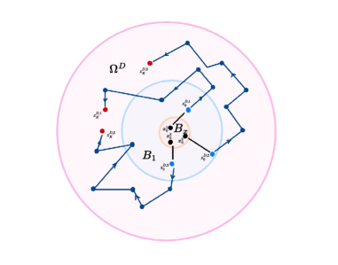
Figure 5: A schematic illustration of the main bounded sets used in the proof. The initial values of the time series used for initializing the NCDE lie in the orange ball of diameter $B_{x}$. The value $z_{0}$ then lies in the blue ball $B_{1}$, whose diameter is upper bounded by a function of $B_{\mathbf{U}},B_{v},B_{x}$ and $L_{\sigma}$. Finally, the trajectories evolves during time but stay within the ball $\Omega^{D}$.

C.4 Proof of Theorem 5.4

We gave bounds for the discretization and approximation biases in Propositions C.1 and C.2. We now have to bound $\sup\limits_{g\in\mathcal{F}_{\Theta}}\Big{[}\mathcal{R}^{D}(g)-\mathcal{R}_{n}^{D}(g)\Big{]}$ and $\sup\limits_{g\in\mathcal{F}_{\Theta}}\Big{[}\mathcal{R}(g)-\mathcal{R}_{n}(g)\Big{]}$ to obtain a bound for the total risk via the total risk decomposition given in Lemma 5.3. It is clear that for any predictor $f_{\theta}$ parameterized by $\theta=(\Phi,\psi,\mathbf{U},v)$ one has

$$\mathcal{R}^{D}(\hat{f}^{D})-\mathcal{R}(\mathbf{f}^{*})$$ (70)

$$\leq\sup\limits_{g\in\mathcal{F}_{\Theta}}\Big{[}\mathcal{R}^{D}(g)-\mathcal{R}_{n}^{D}(g)\Big{]}+\sup\limits_{g\in\mathcal{F}_{\Theta}}\Big{[}\mathcal{R}(g)-\mathcal{R}_{n}(g)\Big{]}$$ (71)

$$\quad+L_{\ell}C^{1}_{\Theta}\lvert D\rvert$$ (72)

$$\quad+L_{\ell}B_{\Phi}\exp(L_{\mathbf{G}^{\star}}L_{x})\Big{[}L_{x}\left\lVert\mathbf{G}_{\psi}-\mathbf{G}^{\star}\right\rVert_{\infty,\Omega}+\left\lVert\varphi^{\star}-\text{NN}_{\mathbf{U},v}\right\rVert_{\infty,B_{x}}\Big{]}$$ (73)

$$\quad+\frac{L_{\ell}M_{\Theta}}{B_{\Phi}}\left\lVert\Phi_{\star}-\Phi\right\rVert.$$ (74)

Now, by a classical symmetrization argument - see for instance Bach (2021), Proposition 4.2 - the obtained bounds on the Rademacher complexity imply that

$$\sup\limits_{g\in\mathcal{F}_{\Theta}}\Big{[}\mathcal{R}(g)-\mathcal{R}_{n}(g)\Big{]}\leq 2\textnormal{Rad}(\mathcal{F}_{\Theta})$$ (75)

and

$$\sup\limits_{g\in\mathcal{F}^{D}_{\Theta}}\Big{[}\mathcal{R}^{D}(g)-\mathcal{R}^{D}_{n}(g)\Big{]}\leq 2\textnormal{Rad}(\mathcal{F}^{D}_{\Theta}).$$ (76)

This gives

$$\sup\limits_{g\in\mathcal{F}_{\Theta}}\Big{[}\mathcal{R}^{D}(g)-\mathcal{R}_{n}^{D}(g)\Big{]}+\sup\limits_{g\in\mathcal{F}_{\Theta}}\Big{[}\mathcal{R}(g)-\mathcal{R}_{n}(g)\Big{]}\leq 4\max\{\textnormal{Rad}(\mathcal{F}^{D}_{\Theta}),\textnormal{Rad}(\mathcal{F}_{\Theta})\}$$ (77)

To finish the proof, notice that since the risk decomposition

$$\mathcal{R}^{D}(\hat{f}^{D})-\mathcal{R}(\mathbf{f}^{*}) \leq\sup\limits_{g\in\mathcal{F}_{\Theta}}\Big{[}\mathcal{R}^{D}(g)-\mathcal{R}_{n}^{D}(g)\Big{]}+\sup\limits_{g\in\mathcal{F}_{\Theta}}\Big{[}\mathcal{R}(g)-\mathcal{R}_{n}(g)\Big{]}$$

$$\quad+\mathcal{R}_{n}^{D}(f)-\mathcal{R}_{n}(f)+\mathcal{R}(f)-\mathcal{R}(\mathbf{f}^{\star})$$

$$\leq 4\max\{\textnormal{Rad}(\mathcal{F}^{D}_{\Theta}),\textnormal{Rad}(\mathcal{F}_{\Theta})\}+C_{\Theta}^{1}\lvert D\rvert$$

$$+L_{\ell}B_{\Phi}\exp(L_{\mathbf{G}^{\star}}L_{x})\Big{[}L_{x}\left\lVert\mathbf{G}_{\psi}-\mathbf{G}^{\star}\right\rVert_{\infty,\Omega}+\left\lVert\varphi^{\star}-\text{NN}_{\mathbf{U},v}\right\rVert_{\infty,B_{x}}\Big{]}$$

$$+\frac{L_{\ell}M_{\Theta}}{B_{\Phi}}\left\lVert\Phi_{\star}-\Phi\right\rVert$$

holds for every $f_{\theta}\in\mathcal{F}_{\Theta}$ parameterized by $(\Phi,\psi,\mathbf{U},v)$, one may take the infimum over all possible predictors in $\mathcal{F}_{\Theta}$. Since this parameter space is compact by definition, the infimum is a minimum and one has

$$\mathcal{R}^{D}(\hat{f}^{D})-\mathcal{R}(\mathbf{f}^{*})$$

$$\leq 4\max\{\textnormal{Rad}(\mathcal{F}^{D}_{\Theta}),\textnormal{Rad}(\mathcal{F}_{\Theta})\}+C_{\Theta}^{1}\lvert D\rvert$$

$$+L_{\ell}B_{\Phi}\exp(L_{\mathbf{G}^{\star}}L_{x})\Big{[}L_{x}\min_{\psi}\left\lVert\mathbf{G}_{\psi}-\mathbf{G}^{\star}\right\rVert_{\infty,\Omega}+\min_{\mathbf{U},v}\left\lVert\varphi^{\star}-\text{NN}_{\mathbf{U},v}\right\rVert_{\infty,B_{x}}\Big{]}$$

$$+\frac{L_{\ell}M_{\Theta}}{B_{\Phi}}\underbrace{\min_{\Phi}\left\lVert\Phi_{\star}-\Phi\right\rVert}_{=0}$$

which concludes the proof.

Appendix D Supplementary proofs

D.1 Proof of Lemma B.1

Take $\mathbf{G}_{\psi}:\mathbb{R}^{p}\to\mathbb{R}^{p\times d}$ a neural vector field and $z,w\in\mathbb{R}^{p}$. Define

$$\mu_{h}(z):=\sigma\Big{(}\mathbf{A}_{h}\sigma\Big{(}\mathbf{A}_{h-1}\sigma\Big{(}\dots\sigma\Big{(}\mathbf{A}_{1}z+\mathbf{b}_{1}\Big{)}\Big{)}+\mathbf{b}_{h-1}\Big{)}+\mathbf{b}_{h}\Big{)}$$

for all $h=2,\dots,q$. One directly has

$$\left\lVert\mathbf{G}_{\psi}(z)-\mathbf{G}_{\psi}(w)\right\rVert =\left\lVert\mu_{q}(z)-\mu_{q}(w)\right\rVert\leq L_{\sigma}\left\lVert\mathbf{A}_{q}\big{(}\mu_{q-1}(z)-\mu_{q-1}(w)\big{)}\right\rVert$$ (78)

$$\leq L_{\sigma}B_{\mathbf{A}}\left\lVert\mu_{q-1}(z)-\mu_{q-1}(w)\right\rVert$$ (79)

$$\leq\dots$$ (80)

$$\leq\Big{(}L_{\sigma}B_{\mathbf{A}}\Big{)}^{q}\left\lVert z-w\right\rVert.$$ (81)

This proves our claim.

D.2 Proof of Lemma B.2

Let $z\in\mathbb{R}^{p}$ and define

$$\mu_{h}(z):=\sigma\Big{(}\mathbf{A}^{1}_{h}\sigma\Big{(}\mathbf{A}^{1}_{h-1}\sigma\Big{(}\dots\sigma\Big{(}\mathbf{A}^{1}_{1}z+\mathbf{b}^{1}_{1}\Big{)}\Big{)}+\mathbf{b}^{1}_{h-1}\Big{)}+\mathbf{b}^{1}_{h}\Big{)}$$

for all $h=2,\dots,q$. One has

$$\left\lVert\mathbf{G}_{\psi}(z)\right\rVert_{\textnormal{op}} =\left\lVert\mu_{q}(z)\right\rVert_{\textnormal{op}}$$ (82)

$$\leq\left\lVert\mu_{q}(z)-\mu_{q}(\mathbf{0})+\mu_{q}(\mathbf{0})\right\rVert$$ (83)

$$\leq\left\lVert\mu_{q}(z)-\mu_{q}(\mathbf{0})\right\rVert+\left\lVert\mu_{q}(\mathbf{0})\right\rVert.$$ (84)

Using Lemma B.1, one has that

$$\left\lVert\mu_{q}(z)-\mu_{q}(\mathbf{0})\right\rVert\leq\Big{(}L_{\sigma}B_{\mathbf{A}}\Big{)}^{q}\left\lVert z\right\rVert.$$ (85)

To finish the proof, one has to bound $\left\lVert\mu_{q}(\mathbf{0})\right\rVert$. Since

$$\left\lVert\mu_{q}(\mathbf{0})\right\rVert=\left\lVert\mu_{q}(\mathbf{0})-\sigma(\mathbf{0})\right\rVert \leq L_{\sigma}\left\lVert\mathbf{A}_{q}\mu_{q-1}(\mathbf{0})\right\rVert+L_{\sigma}B_{\mathbf{b}}$$ (86)

$$\leq L_{\sigma}B_{\mathbf{A}}\left\lVert\mu_{q-1}(\mathbf{0})\right\rVert+L_{\sigma}B_{\mathbf{b}},$$ (87)

using Lemma A.6 yields

$$\left\lVert\mu_{q}(\mathbf{0})\right\rVert \leq\big{(}L_{\sigma}B_{\mathbf{A}}\big{)}^{q-1}\left\lVert\sigma(\mathbf{b}_{1})\right\rVert+L_{\sigma}B_{\mathbf{b}}\sum\limits_{j=0}^{q-2}\big{(}L_{\sigma}B_{\mathbf{A}}\big{)}^{j}$$ (88)

$$\leq L_{\sigma}B_{\mathbf{b}}\sum\limits_{j=0}^{q-1}\big{(}L_{\sigma}B_{\mathbf{A}}\big{)}^{j}$$ (89)

$$=L_{\sigma}B_{\mathbf{b}}\frac{\big{(}L_{\sigma}B_{\mathbf{A}}\big{)}^{q}-1}{L_{\sigma}B_{\mathbf{A}}-1}.$$ (90)

Combining everything yields

$$\left\lVert\mathbf{G}_{\psi}(z)\right\rVert_{\textnormal{op}}\leq\Big{(}L_{\sigma}B_{\mathbf{A}}\Big{)}^{q}\left\lVert z\right\rVert+L_{\sigma}B_{\mathbf{b}}\frac{\big{(}L_{\sigma}B_{\mathbf{A}}\big{)}^{q}-1}{L_{\sigma}B_{\mathbf{A}}-1}.$$ (91)

D.3 Proof of Lemma B.3

Define

$$\mu^{1}_{h}(z):=\sigma\Big{(}\mathbf{A}^{1}_{h}\sigma\Big{(}\mathbf{A}^{1}_{h-1}\sigma\Big{(}\dots\sigma\Big{(}\mathbf{A}^{1}_{1}z+\mathbf{b}^{1}_{1}\Big{)}\Big{)}+\mathbf{b}^{1}_{h-1}\Big{)}+\mathbf{b}^{1}_{h}\Big{)}$$

and

$$\mu^{2}_{h}(z):=\sigma\Big{(}\mathbf{A}^{2}_{h}\sigma\Big{(}\mathbf{A}^{2}_{h-1}\sigma\Big{(}\dots\sigma\Big{(}\mathbf{A}^{2}_{1}z+\mathbf{b}^{2}_{1}\Big{)}\Big{)}+\mathbf{b}^{2}_{h-1}\Big{)}+\mathbf{b}^{2}_{h}\Big{)}$$

for all $h=2\dots,q$. The indice $h$ therefore refers to the depth of the neural vector field.

For the first hidden layer, one has

$$\left\lVert\sigma\Big{(}\mathbf{A}^{1}_{1}z+\mathbf{b}^{1}_{1}\Big{)}-\sigma\Big{(}\mathbf{A}^{2}_{1}z+\mathbf{b}^{2}_{1}\Big{)}\right\rVert \leq L_{\sigma}\left\lVert\mathbf{b}^{1}_{1}-\mathbf{b}^{2}_{1}\right\rVert+L_{\sigma}\left\lVert\mathbf{A}^{1}_{1}z-\mathbf{A}^{2}_{1}z\right\rVert$$ (92)

$$\leq L_{\sigma}\left\lVert\mathbf{b}^{1}_{1}-\mathbf{b}^{2}_{1}\right\rVert+L_{\sigma}\left\lVert\mathbf{A}^{1}_{1}-\mathbf{A}^{2}_{1}\right\rVert\left\lVert z\right\rVert.$$ (93)

Similarly, for any $h=2,\dots,q$, one has

$$\left\lVert\mu^{1}_{h}(z)-\mu^{2}_{h}(z)\right\rVert =\left\lVert\sigma\big{(}\mathbf{A}^{1}_{h}\mu^{1}_{h-1}(z)+\mathbf{b}^{1}_{h}\big{)}-\sigma\big{(}\mathbf{A}^{2}_{h}\mu^{2}_{h-1}(z)+\mathbf{b}^{2}_{h}\big{)}\right\rVert$$ (94)

$$\leq L_{\sigma}\left\lVert\mathbf{A}^{1}_{h}\mu^{1}_{h-1}(z)-\mathbf{A}^{2}_{h}\mu^{2}_{h-1}(z)\right\rVert+L_{\sigma}\left\lVert\mathbf{b}^{1}_{h}-\mathbf{b}^{2}_{h}\right\rVert$$ (95)

$$\leq L_{\sigma}\left\lVert\Big{(}\mathbf{A}^{1}_{h}-\mathbf{A}^{2}_{h}+\mathbf{A}^{2}_{h}\Big{)}\mu^{1}_{h-1}(z)-\mathbf{A}^{2}_{h}\mu^{2}_{h-1}(z)\right\rVert+L_{\sigma}\left\lVert\mathbf{b}^{1}_{h}-\mathbf{b}^{2}_{h}\right\rVert$$ (96)

$$\leq L_{\sigma}\left\lVert\mathbf{A}^{1}_{h}-\mathbf{A}_{h}^{2}\right\rVert\left\lVert\mu^{1}_{h-1}(z)\right\rVert+L_{\sigma}\left\lVert\mathbf{A}_{h}^{2}\right\rVert\left\lVert\mu^{1}_{h-1}(z)-\mu^{2}_{h-1}(z)\right\rVert$$ (97)

$$+L_{\sigma}\left\lVert\mathbf{b}^{1}_{h}-\mathbf{b}^{2}_{h}\right\rVert.$$ (98)

Since we have assumed that $\left\lVert\mathbf{A}^{2}_{q}\right\rVert\leq B_{\mathbf{A}}$, this yields

$$\left\lVert\mu^{1}_{h}(z)-\mu^{2}_{h}(z)\right\rVert \leq L_{\sigma}\left\lVert\mathbf{A}^{1}_{h}-\mathbf{A}_{h}^{2}\right\rVert\left\lVert\mu^{1}_{h-1}(z)\right\rVert+L_{\sigma}B_{\mathbf{A}}\left\lVert\mu^{1}_{h-1}(z)-\mu^{2}_{h-1}(z)\right\rVert$$ (99)

$$+L_{\sigma}\left\lVert\mathbf{b}^{1}_{h}-\mathbf{b}_{h}^{2}\right\rVert.$$ (100)

We may now use Lemma A.6 to get that

$$\left\lVert\mu^{1}_{q}(z)-\mu^{2}_{q}(z)\right\rVert \leq L_{\sigma}\sum\limits_{j=2}^{q}\Big{[}\left\lVert\mathbf{A}_{j}^{1}-\mathbf{A}_{j}^{2}\right\rVert\left\lVert\mu^{1}_{j-1}(z)\right\rVert+\left\lVert\mathbf{b}_{j}^{1}-\mathbf{b}_{j}^{2}\right\rVert\Big{]}\big{(}L_{\sigma}B_{\mathbf{A}}\big{)}^{q-j}$$ (101)

$$+\big{(}L_{\sigma}B_{\mathbf{A}}\big{)}^{q-1}\left\lVert\sigma\Big{(}\mathbf{A}^{1}_{1}z+\mathbf{b}^{1}_{1}\Big{)}-\sigma\Big{(}\mathbf{A}^{2}_{1}z+\mathbf{b}^{2}_{1}\Big{)}\right\rVert$$ (102)

$$\leq L_{\sigma}\sum\limits_{j=2}^{q}\Big{[}\left\lVert\mathbf{A}_{j}^{1}-\mathbf{A}_{j}^{2}\right\rVert\left\lVert\mu^{1}_{j-1}(z)\right\rVert+\left\lVert\mathbf{b}_{j}^{1}-\mathbf{b}_{j}^{2}\right\rVert\Big{]}\big{(}L_{\sigma}B_{\mathbf{A}}\big{)}^{q-j}$$ (103)

$$+L_{\sigma}^{q}B_{\mathbf{A}}^{q-1}\left\lVert\mathbf{b}^{1}_{1}-\mathbf{b}^{2}_{1}\right\rVert+L_{\sigma}^{q}B_{\mathbf{A}}^{q-1}\left\lVert\mathbf{A}^{1}_{1}-\mathbf{A}^{2}_{1}\right\rVert\left\lVert z\right\rVert.$$ (104)

We may now use Lemma B.2. For all $h=1,\dots,q$, one has

$$\left\lVert\mu^{1}_{h}(z)\right\rVert\leq\alpha_{h}\left\lVert z\right\rVert+\beta_{h}$$ (105)

with

$$\alpha_{h}:=\big{(}L_{\sigma}B_{\mathbf{A}}\big{)}^{h}\text{ and }\beta_{h}:=L_{\sigma}B_{\mathbf{b}}\frac{\big{(}L_{\sigma}B_{\mathbf{A}}\big{)}^{h}-1}{L_{\sigma}B_{\mathbf{A}}-1}.$$ (106)

We furthermore let $\alpha_{0}:=1$ and $\beta_{0}=0$. One then has

$$\left\lVert\mu^{1}_{q}(z)-\mu^{2}_{q}(z)\right\rVert$$ (107)

$$\leq L_{\sigma}\sum\limits_{j=1}^{q}\Big{[}\left\lVert\mathbf{A}_{j}^{1}-\mathbf{A}_{j}^{2}\right\rVert\big{(}\alpha_{j-1}\left\lVert z\right\rVert+\beta_{j-1}\big{)}+\left\lVert\mathbf{b}_{j}^{1}-\mathbf{b}_{j}^{2}\right\rVert\Big{]}\big{(}L_{\sigma}B_{\mathbf{A}}\big{)}^{q-j}$$ (108)

and thus

$$\left\lVert\mathbf{G}_{\psi^{1}}(z)-\mathbf{G}_{\psi^{2}}(z)\right\rVert_{\textnormal{op}}\leq\sum\limits_{j=1}^{q}\Big{[}C_{\mathbf{b}}^{j}\left\lVert\mathbf{b}_{j}^{1}-\mathbf{b}_{j}^{2}\right\rVert+C_{\mathbf{A}}^{j}(z)\left\lVert\mathbf{A}^{1}_{j}-\mathbf{A}^{2}_{j}\right\rVert\Big{]}$$ (109)

with $C_{\mathbf{A}}^{j}(z):=\big{(}L_{\sigma}B_{\mathbf{A}}\big{)}^{q-j}L_{\sigma}\Big{(}\alpha_{j-1}\left\lVert z\right\rVert+\beta_{j-1}\Big{)}$ and $C_{\mathbf{b}}^{j}=\big{(}L_{\sigma}B_{\mathbf{A}}\big{)}^{q-j}L_{\sigma}$. This proves our claim.

D.4 Proof of Lemma 3.3 and Lemma 5.2

We recall that $\left\lVert W\right\rVert_{\textnormal{op}}:=\max\limits_{\left\lVert x\right\rVert=1}\left\lVert Wx\right\rVert$, and that $\left\lVert W\right\rVert_{\textnormal{op}}\leq\left\lVert W\right\rVert$, which means that $\left\lVert Wx\right\rVert\leq\left\lVert W\right\rVert\left\lVert x\right\rVert$ for all $x$. We first prove this result for a general CDE

$$dz_{t}=\mathbf{F}(z_{t})dx_{t}$$

with initial condition $z_{0}\in\mathbb{R}^{p}$, where the driving path $x$ is supposed to be continuous of bounded variation (or piecewise constant with a finite number of discontinuities.)

By definition,

$$z_{t}=z_{0}+\int_{0}^{t}\mathbf{F}(z_{t})dx_{t}.$$ (110)

Taking norms, this yields

$$\left\lVert z_{t}\right\rVert\leq\left\lVert z_{0}\right\rVert+\int_{0}^{t}\left\lVert\mathbf{F}(z_{t})\right\rVert_{\textnormal{op}}\left\lVert dx_{t}\right\rVert.$$ (111)

Notice that since we have assumed $\mathbf{F}$ to be Lipschitz, one has for all $z\in\mathbb{R}^{p}$

$$\left\lVert\mathbf{F}(z)\right\rVert_{\textnormal{op}} \leq\left\lVert\mathbf{F}(z)-\mathbf{F}(0)\right\rVert_{\textnormal{op}}+\left\lVert\mathbf{F}(0)\right\rVert_{\textnormal{op}}$$ (112)

$$\leq\left\lVert\mathbf{F}(z)-\mathbf{F}(0)\right\rVert+\left\lVert\mathbf{F}(0)\right\rVert_{\textnormal{op}}$$ (113)

$$\leq L_{\mathbf{F}}\left\lVert z\right\rVert+\left\lVert\mathbf{F}(0)\right\rVert_{\textnormal{op}},$$ (114)

where the last inequality follows from the fact that $\mathbf{F}$ is Lipschitz. It follows that

$$\left\lVert z_{t}\right\rVert\leq\left\lVert z_{0}\right\rVert+\int_{0}^{t}(L_{\mathbf{F}}\left\lVert z_{t}\right\rVert+\left\lVert\mathbf{F}(0)\right\rVert_{\textnormal{op}})\left\lVert dx_{t}\right\rVert.$$ (115)

Using the fact that $\int_{0}^{t}\left\lVert dx_{s}\right\rVert=\left\lVert x\right\rVert_{\textnormal{1-var},[0,t]}$, one gets

$$\left\lVert z_{t}\right\rVert\leq\left\lVert z_{0}\right\rVert+\left\lVert\mathbf{F}(0)\right\rVert_{\textnormal{op}}\left\lVert x\right\rVert_{\textnormal{1-var},[0,t]}+L_{\mathbf{F}}\int_{0}^{t}\left\lVert z_{s}\right\rVert\left\lVert dx_{s}\right\rVert.$$ (116)

Applying Gronwall’s Lemma for CDEs yields

$$\left\lVert z_{t}\right\rVert\leq\Big{(}\left\lVert z_{0}\right\rVert+\left\lVert\mathbf{F}(0)\right\rVert_{\textnormal{op}}\left\lVert x\right\rVert_{\textnormal{1-var},[0,t]}\Big{)}\exp\big{(}L_{\mathbf{F}}\left\lVert x\right\rVert_{\textnormal{1-var},[0,t]}\big{)}.$$ (117)

Now, turning to the generative CDE equation 5, we obtain as a consequence that

$$\lvert y\rvert\leq B_{\Phi}\Big{(}B_{\varphi}^{\star}+\left\lVert\mathbf{G}^{\star}(0)\right\rVert_{\textnormal{op}}L_{x}\Big{)}\exp\big{(}L_{\mathbf{G}^{\star}}L_{x}\big{)}+M_{\varepsilon},$$ (118)

since $y$ is the sum of a linear transformation of the endpoint of a CDE an a noise term $\varepsilon$ bounded by $M_{\varepsilon}$. This proves Lemma 5.2.

Turning now to $f_{\theta}\in\mathcal{F}_{\Theta}$, one has that

$$\lvert f_{\theta}(x)\rvert=\lvert\Phi^{\top}z_{1}\rvert\leq\left\lVert\Phi\right\rVert\left\lVert z_{1}\right\rVert\leq B_{\Phi}\left\lVert z_{1}\right\rVert$$ (119)

and since $z_{1}$ is the solution of a NCDE, we can directly leverage the previous result to bound $\left\lVert z_{1}\right\rVert$, which yields

$$\left\lVert z_{1}\right\rVert\leq L_{\sigma}\exp\big{(}(B_{\mathbf{A}}L_{\sigma})^{q}L_{x}\big{)}\Big{(}B_{\mathbf{U}}B_{x}+B_{v}+\kappa_{\Theta}(\mathbf{0})L_{x}\Big{)}.$$ (120)

As a direct consequence, one has

$$\lvert f_{\theta}(x)\rvert\leq B_{\Phi}L_{\sigma}\exp\big{(}(B_{\mathbf{A}}L_{\sigma})^{q}L_{x}\big{)}\Big{(}B_{\mathbf{U}}B_{x}+B_{v}+\kappa_{\Theta}(\mathbf{0})L_{x}\Big{)}<\infty.$$ (121)

We now turn to $f_{\theta}(\mathbf{x}^{D})$. Bounding the value of $z^{D}_{1}$ can be done by applying this lemma to the values of $z^{D}$ at points in $D$, since it is constant between those points. The proof leverages the discrete version of Gronwall’s Lemma, stated in Lemma A.5. One has

$$\left\lVert z_{t_{k}}\right\rVert\leq\left\lVert z_{0}\right\rVert+\sum\limits_{l=0}^{k-1}\left\lVert\mathbf{G}_{\psi}(z_{t_{l}})\Delta x_{t_{l+1}}\right\rVert\leq\sum\limits_{l=0}^{k-1}\left\lVert\mathbf{G}_{\psi}(z_{t_{l}})\right\rVert\left\lVert\Delta x_{t_{l+1}}\right\rVert,$$ (122)

for all $k=1,\dots,K$. Now, since

$$\left\lVert\mathbf{G}_{\psi}(z_{t_{l}})\right\rVert\leq\big{(}L_{\sigma}B_{\mathbf{A}}\big{)}^{q}\left\lVert z_{t_{l}}\right\rVert+L_{\sigma}B_{\mathbf{b}}\frac{\big{(}L_{\sigma}B_{\mathbf{A}}\big{)}^{q}-1}{L_{\sigma}B_{\mathbf{A}}-1}$$ (123)

one has

$$\left\lVert z_{t_{k}}\right\rVert \leq\left\lVert z_{0}\right\rVert+L_{\sigma}B_{\mathbf{b}}\frac{\big{(}L_{\sigma}B_{\mathbf{A}}\big{)}^{q}-1}{L_{\sigma}B_{\mathbf{A}}}\sum\limits_{l=0}^{k-1}\left\lVert\Delta x_{t_{l+1}}\right\rVert+\big{(}L_{\sigma}B_{\mathbf{A}}\big{)}^{q}\sum\limits_{l=0}^{k-1}\left\lVert z_{t_{l}}\right\rVert\left\lVert\Delta x_{l+1}\right\rVert$$ (124)

$$\leq\left\lVert z_{0}\right\rVert+L_{\sigma}B_{\mathbf{b}}\frac{\big{(}L_{\sigma}B_{\mathbf{A}}\big{)}^{q}-1}{L_{\sigma}B_{\mathbf{A}}}L_{x}+\big{(}L_{\sigma}B_{\mathbf{A}}\big{)}^{q}\sum\limits_{l=0}^{k-1}\left\lVert z_{t_{l}}\right\rVert\left\lVert\Delta x_{l+1}\right\rVert$$ (125)

and one gets by the discrete Gronwall Lemma that

$$\left\lVert z^{D}_{t_{k}}\right\rVert \leq\Big{(}\left\lVert z_{0}\right\rVert+L_{\sigma}B_{\mathbf{b}}\frac{\big{(}L_{\sigma}B_{\mathbf{A}}\big{)}^{q}-1}{L_{\sigma}B_{\mathbf{A}}}L_{x}\Big{)}\prod\limits_{l=0}^{k-1}\Big{(}1+\big{(}L_{\sigma}B_{\mathbf{A}}\big{)}^{q}\left\lVert\Delta x_{t_{l+1}}\right\rVert\Big{)}$$ (126)

$$\leq\Big{(}\left\lVert z_{0}\right\rVert+L_{\sigma}B_{\mathbf{b}}\frac{\big{(}L_{\sigma}B_{\mathbf{A}}\big{)}^{q}-1}{L_{\sigma}B_{\mathbf{A}}}L_{x}\Big{)}\prod\limits_{l=0}^{k-1}\Big{(}1+\big{(}L_{\sigma}B_{\mathbf{A}}\big{)}^{q}L_{x}\lvert D\rvert\Big{)}$$ (127)

since $\left\lVert\Delta x_{t_{l+1}}\right\rVert\leq L_{x}\lvert t_{l+1}-t_{l}\rvert\leq L_{x}\lvert D\rvert$, and finally

$$\left\lVert z^{D}_{t_{k}}\right\rVert \leq\Big{(}L_{\sigma}B_{\mathbf{U}}B_{x}+L_{\sigma}B_{v}+L_{\sigma}B_{\mathbf{b}}\frac{\big{(}L_{\sigma}B_{\mathbf{A}}\big{)}^{q}-1}{L_{\sigma}B_{\mathbf{A}}}L_{x}\Big{)}\prod\limits_{l=0}^{k-1}\Big{(}1+\big{(}L_{\sigma}B_{\mathbf{A}}\big{)}^{q}L_{x}\lvert D\rvert\Big{)}$$ (128)

In the end, this gets us that

$$\lvert f_{\theta}(\mathbf{x}^{D})\rvert \leq B_{\Phi}L_{\sigma}\Big{(}L_{\sigma}B_{\mathbf{U}}B_{x}+B_{v}+L_{\sigma}B_{\mathbf{b}}\frac{\big{(}L_{\sigma}B_{\mathbf{A}}\big{)}^{q}-1}{L_{\sigma}B_{\mathbf{A}}}L_{x}\Big{)}\prod\limits_{l=0}^{K-1}\Big{(}1+\big{(}L_{\sigma}B_{\mathbf{A}}\big{)}^{q}L_{x}\lvert D\rvert\Big{)}$$ (129)

$$=B_{\Phi}L_{\sigma}\Big{(}L_{\sigma}B_{\mathbf{U}}B_{x}+B_{v}+L_{\sigma}B_{\mathbf{b}}\frac{\big{(}L_{\sigma}B_{\mathbf{A}}\big{)}^{q}-1}{L_{\sigma}B_{\mathbf{A}}}L_{x}\Big{)}\Big{(}1+\big{(}L_{\sigma}B_{\mathbf{A}}\big{)}^{q}L_{x}\lvert D\rvert\Big{)}^{K}.$$ (130)

Note that by Gronwall’s Lemma, one also has the less tighter bound

$$\lvert f_{\theta}(\mathbf{x}^{D})\rvert\leq B_{\Phi}L_{\sigma}\exp\big{(}(B_{\mathbf{A}}L_{\sigma})^{q}L_{x}\big{)}\Big{(}B_{\mathbf{U}}B_{x}+B_{v}+\kappa_{\Theta}(\mathbf{0})L_{x}\Big{)}.$$ (131)

This concludes the proof.

D.5 Proof of Proposition B.4

We first consider a general CDE

$$dz_{t}=\mathbf{F}(z_{t})dx_{t}$$ (132)

with initial condition $z_{0}\in\mathbb{R}^{p}$. Take $s,r\in[0,t]$. By definition,

$$\left\lVert z_{r}-z_{s}\right\rVert =\left\lVert\int_{s}^{r}\mathbf{F}(z_{u})dx_{u}\right\rVert$$ (133)

$$=\left\lVert\int_{s}^{r}\mathbf{F}\big{(}z_{u}-z_{s}+z_{s}\big{)}dx_{u}\right\rVert$$ (134)

$$\leq\int_{s}^{r}\big{(}L_{\mathbf{F}}\left\lVert z_{u}-z_{s}+z_{s}\right\rVert+\left\lVert\mathbf{F}(0)\right\rVert_{\textnormal{op}}\big{)}\left\lVert dx_{u}\right\rVert$$ (135)

$$\leq\int_{s}^{r}\big{(}L_{\mathbf{F}}\left\lVert z_{u}-z_{s}\right\rVert+L_{\mathbf{F}}\left\lVert z_{s}\right\rVert+\left\lVert\mathbf{F}(0)\right\rVert_{\textnormal{op}}\big{)}\left\lVert dx_{u}\right\rVert$$ (136)

$$=\big{(}L_{\mathbf{F}}\left\lVert z_{s}\right\rVert+\left\lVert\mathbf{F}(0)\right\rVert_{\textnormal{op}}\big{)}\left\lVert x\right\rVert_{\textnormal{1-var},[s,r]}+L_{\mathbf{F}}\int_{s}^{r}\left\lVert z_{u}-z_{s}\right\rVert\left\lVert dx_{u}\right\rVert.$$ (137)

Now since $z_{s}$ is the solution of a CDE evaluated at $s$, it can be bounded by Lemma 3.3 by

$$\left\lVert z_{s}\right\rVert\leq\big{(}\left\lVert z_{0}\right\rVert+\left\lVert\mathbf{F}(0)\right\rVert_{\textnormal{op}}\left\lVert x\right\rVert_{\textnormal{1-var},[0,s]}\big{)}\exp(L_{\mathbf{F}}\left\lVert x\right\rVert_{\textnormal{1-var},[0,s]}).$$ (138)

This means that

$$\left\lVert z_{r}-z_{s}\right\rVert$$ (139)

$$\leq\Big{[}L_{\mathbf{F}}\big{(}\left\lVert z_{0}\right\rVert+\left\lVert\mathbf{F}(0)\right\rVert_{\textnormal{op}}\left\lVert x\right\rVert_{\textnormal{1-var},[0,s]}\big{)}\exp(L_{\mathbf{F}}\left\lVert x\right\rVert_{\textnormal{1-var},[0,s]})+\left\lVert\mathbf{F}(0)\right\rVert_{\textnormal{op}}\Big{]}\left\lVert x\right\rVert_{\textnormal{1-var},[s,r]}$$ (140)

$$+L_{\mathbf{F}}\int_{s}^{r}\left\lVert z_{u}-z_{s}\right\rVert\left\lVert dx_{u}\right\rVert.$$ (141)

We may now use Gronwall’s Lemma and the fact that $\left\lVert x\right\rVert_{\textnormal{1-var},[0,s]}\leq L_{x}$ for all $s\in[0,1]$ to obtain that

$$\left\lVert z_{r}-z_{s}\right\rVert \leq\Bigg{[}L_{\mathbf{F}}\big{(}\left\lVert z_{0}\right\rVert+\left\lVert\mathbf{F}(0)\right\rVert_{\textnormal{op}}L_{x}\big{)}\exp(L_{\mathbf{F}}L_{x})+\left\lVert\mathbf{F}(0)\right\rVert_{\textnormal{op}}\Bigg{]}\exp(L_{\mathbf{F}}L_{x})\left\lVert x\right\rVert_{\textnormal{1-var},[s,r]}.$$ (142)

and thus

$$\left\lVert z_{r}-z_{s}\right\rVert\leq C_{1}(\mathbf{F})\left\lVert x\right\rVert_{\textnormal{1-var},[s,r]}.$$ (143)

This means that the variations of $z$ on arbitrary intervals $[r,s]$ are bounded by the variations of $x$ on the same interval, times an interval independent constant.

From this, we may immediately conclude that

$$\left\lVert z\right\rVert_{\textnormal{1-var},[0,t]}\leq C_{1}(\mathbf{F})\left\lVert x\right\rVert_{\textnormal{1-var},[0,t]},$$ (144)

which concludes the proof for a general CDE. We now turn to $f_{\theta}\in\mathcal{F}_{\Theta}$. The previous result allows to bound the total variation of a CDE and thus of the trajectory of the latent state. Using this proposition with

$$C_{1}(\mathbf{G}_{\psi}):=$$ (145)

$$\Bigg{[}\big{(}L_{\sigma}B_{\mathbf{A}}\big{)}^{q}\Big{(}L_{\sigma}B_{\mathbf{U}}B_{x}+L_{\sigma}B_{v}+\kappa_{\Theta}(\mathbf{0})L_{x}\Big{)}\exp\big{(}(L_{\sigma}B_{\mathbf{A}})^{q}L_{x})+\kappa_{\Theta}(\mathbf{0})\Bigg{]}\exp\big{(}(L_{\sigma}B_{\mathbf{A}})^{q}L_{x}\big{)}$$ (146)

$$=\Big{[}\Big{(}L_{\sigma}B_{\mathbf{A}}\Big{)}^{q}\frac{1}{B_{\Phi}}M_{\Theta}+\kappa_{\Theta}(\mathbf{0})\Big{]}\exp((L_{\sigma}B_{\mathbf{A}})^{q}L_{x})$$ (147)

yields

$$\left\lVert z\right\rVert_{\textnormal{1-var}}\leq C_{1}(\mathbf{G}_{\psi})L_{x}.$$ (148)

This concludes the proof for $f_{\theta}$ with continuous input. For discretized inputs, the proof follows readily with constant $M_{\Theta}^{D}$.

D.6 Proof of Theorem B.5

For all $t\in[0,1]$, one has the decomposition

$$w_{t}-v_{t} =w_{0}-v_{0}+\int_{0}^{t}\mathbf{F}(w_{s})dx_{s}-\int_{0}^{t}\mathbf{G}(v_{s})dr_{s}$$ (149)

$$=w_{0}-v_{0}+\int_{0}^{t}\big{(}\mathbf{F}(w_{s})-\mathbf{F}(v_{s})\big{)}dx_{s}+\int_{0}^{t}\mathbf{F}(v_{s})dx_{s}-\int_{0}^{t}\mathbf{G}(v_{s})dr_{s}$$ (150)

$$=w_{0}-v_{0}$$ (151)

$$+\int_{0}^{t}\big{(}\mathbf{F}(w_{s})-\mathbf{F}(v_{s})\big{)}dx_{s}$$ (152)

$$+\int_{0}^{t}\mathbf{F}(v_{s})d(x_{s}-r_{s})$$ (153)

$$+\int_{0}^{t}\big{(}\mathbf{F}(v_{s})-\mathbf{G}(v_{s})\big{)}dr_{s}.$$ (154)

We control every one of these terms separately and conclude by applying Gronwall’s Lemma. Writing

$$A:=\left\lVert\int_{0}^{t}\big{(}\mathbf{F}(w_{s})-\mathbf{F}(v_{s})\big{)}dx_{s}\right\rVert,$$

$$B:=\left\lVert\int_{0}^{t}\mathbf{F}(v_{s})d(x_{s}-r_{s})\right\rVert,$$

$$C:=\left\lVert\int_{0}^{t}\big{(}\mathbf{F}(v_{s})-\mathbf{G}(v_{s})\big{)}dr_{s}\right\rVert$$

it is clear that

$$\left\lVert w_{t}-z_{t}\right\rVert\leq\left\lVert w_{0}-z_{0}\right\rVert+A+B+C.$$ (155)

Control of the term $A$.

One has

$$A\leq\int_{0}^{t}\left\lVert\mathbf{F}(w_{s})-\mathbf{F}(v_{s})\right\rVert_{\textnormal{op}}\left\lVert dx_{s}\right\rVert.$$ (156)

Since $F$ is $L_{\mathbf{F}}$-Lipschitz, this gives

$$A\leq L_{\mathbf{F}}\int_{0}^{t}\left\lVert w_{s}-v_{s}\right\rVert\left\lVert dx_{s}\right\rVert.$$ (157)

Control of the term $B$.

One gets using integration by parts

$$\int_{0}^{t}\mathbf{F}(v_{s})d(x_{s}-r_{s})=(x_{t}-r_{t})-(x_{0}-r_{0})-\int_{0}^{t}(x_{s}-r_{s})^{\top}d\mathbf{F}(v_{s}).$$ (158)

This gives

$$B\leq\left\lVert x_{0}-r_{0}\right\rVert+\left\lVert x-r\right\rVert_{\infty,[0,t]}(1+\left\lVert\mathbf{F}(v)\right\rVert_{\textnormal{1-var},[0,t]}).$$ (159)

Since $\mathbf{F}$ is $L_{\mathbf{F}}$-Lipschitz, one gets

$$\left\lVert\mathbf{F}(v)\right\rVert_{\textnormal{1-var},[0,t]}\leq L_{\mathbf{F}}\left\lVert v\right\rVert_{\textnormal{1-var},[0,t]}.$$ (160)

Since $v$ is the solution to a CDE, we can resort to Proposition B.4 to bound its total variation. This yields

$$\left\lVert v\right\rVert_{\textnormal{1-var},[0,t]}\leq C_{1}(L_{\mathbf{F}},\mathbf{F},L_{r})\left\lVert r\right\rVert_{\textnormal{1-var},[0,t]}$$ (161)

and finally

$$B\leq\left\lVert x_{0}-r_{0}\right\rVert+\left\lVert x-r\right\rVert_{\infty,[0,t]}(1+L_{\mathbf{F}}C_{1}(L_{\mathbf{F}},\mathbf{F},L_{x})\left\lVert r\right\rVert_{\textnormal{1-var},[0,t]}).$$ (162)

Control of the term $C$.

Finally, we get that

$$C \leq\int_{0}^{t}\left\lVert\mathbf{F}(v_{s})-\mathbf{G}(v_{s})\right\rVert_{\textnormal{op}}\left\lVert dr_{s}\right\rVert$$ (163)

$$\leq\max_{v\in\Omega}\left\lVert\mathbf{F}(v)-\mathbf{G}(v)\right\rVert_{\textnormal{op}}L_{r}$$ (164)

where we recall that $\Omega$ is the closed ball

$$\Omega=\big{\{}u\in\mathbb{R}^{p}\,|\,\left\lVert u\right\rVert\leq(\left\lVert v_{0}\right\rVert+\left\lVert\mathbf{G}(0)\right\rVert L_{r})\exp(L_{\mathbf{G}}L_{r})\big{\}}.$$

Indeed, since $v$ is the solution of a CDE, its norm at any time $t\in[0,1]$ is bounded as stated in Lemma 3.3. One can therefore bound the difference $\left\lVert\mathbf{F}(v_{s})-\mathbf{G}(v_{s})\right\rVert_{\textnormal{op}}$ by considering all possible values of $v$.

Putting everything together.

Combining the obtained bounds on all terms, one is left with

$$\left\lVert w_{t}-v_{t}\right\rVert \leq\left\lVert w_{0}-v_{0}\right\rVert$$ (165)

$$\quad+\left\lVert x_{0}-r_{0}\right\rVert+\left\lVert x-r\right\rVert_{\infty,[0,t]}(1+L_{\mathbf{F}}L_{r}C_{1}(L_{\mathbf{F}},\mathbf{F},L_{x}))$$ (166)

$$\quad+L_{r}\max_{v\in\Omega}\left\lVert\mathbf{F}(v)-\mathbf{G}(v)\right\rVert_{\textnormal{op}}$$ (167)

$$\quad+L_{\mathbf{F}}\int_{0}^{t}\left\lVert w_{s}-v_{s}\right\rVert\left\lVert dx_{s}\right\rVert.$$ (168)

The proof is concluded by using Gronwall’s Lemma A.4. If the path $(x_{t})$ is continuous, we resort to its continuous version. If it is piecewise constant, we use its discrete version. The path $(\left\lVert w_{t}-v_{t}\right\rVert)_{t}$ only needs to be measurable and bounded. There are no assumptions on its continuity. This finally yields

$$\left\lVert w_{t}-v_{t}\right\rVert \leq\Bigg{(}\left\lVert w_{0}-v_{0}\right\rVert+\left\lVert x_{0}-r_{0}\right\rVert$$ (169)

$$\quad+\left\lVert x-r\right\rVert_{\infty,[0,t]}\big{(}1+L_{\mathbf{F}}L_{r}C_{1}(L_{\mathbf{F}},\mathbf{F},L_{x})\big{)}+\max_{v\in\Omega}\left\lVert\mathbf{F}(v)-\mathbf{G}(v)\right\rVert_{\textnormal{op}}L_{r}\Bigg{)}$$ (170)

$$\quad\times\exp(L_{\mathbf{F}}L_{x}).$$ (171)

Now, notice that in our proof, the two CDEs are exchangeable. This means that we immediately get the alternative bound

$$\left\lVert w_{t}-v_{t}\right\rVert \leq\Bigg{(}\left\lVert w_{0}-v_{0}\right\rVert+\left\lVert x_{0}-r_{0}\right\rVert$$ (172)

$$\quad+\left\lVert x-r\right\rVert_{\infty,[0,t]}\big{(}1+L_{\mathbf{G}}L_{x}C_{1}(L_{\mathbf{G}},\mathbf{G},L_{r})\big{)}+\max_{v\in\Omega}\left\lVert\mathbf{F}(v)-\mathbf{G}(v)\right\rVert_{\textnormal{op}}L_{x}\Bigg{)}$$ (173)

$$\quad\times\exp(L_{\mathbf{G}}L_{r})$$ (174)

where we recall that

$$\Omega=\big{\{}u\in\mathbb{R}^{p}\,|\,\left\lVert u\right\rVert\leq(\left\lVert w_{0}\right\rVert+\left\lVert\mathbf{F}(0)\right\rVert L_{x})\exp(L_{\mathbf{F}}L_{x})\big{\}}.$$

D.7 Proof of Theorem B.6

Proof for continuous inputs.

One has

$$\lvert f_{\theta_{1}}(x)-f_{\theta_{2}}(x)\rvert=\left\lVert\Phi_{1}^{\top}z^{1}_{1}-\Phi_{2}^{\top}z^{2}_{1}\right\rVert\leq\left\lVert\Phi_{1}-\Phi_{2}\right\rVert\left\lVert z^{1}_{1}\right\rVert+B_{\Phi}\left\lVert z_{1}^{1}-z_{1}^{2}\right\rVert.$$ (175)

Using Theorem B.5, one gets that

$$\left\lVert z_{1}^{1}-z_{1}^{2}\right\rVert\leq\exp\big{(}(L_{\sigma}B_{\mathbf{A}})^{q}L_{x}\big{)}\Big{(}\left\lVert z_{0}^{1}-z_{0}^{2}\right\rVert+L_{x}\left\lVert\mathbf{G}_{\psi^{1}}-\mathbf{G}_{\psi^{2}}\right\rVert_{\infty,\Omega}\Big{)},$$ (176)

where

$$\Omega=\big{\{}u\in\mathbb{R}^{p}\,|\,\left\lVert u\right\rVert\leq\big{(}L_{\sigma}(B_{\mathbf{U}}B_{x}+B_{v})+\left\lVert\mathbf{G}_{\psi}(\mathbf{0})\right\rVert_{\textnormal{op}}\big{)}\exp\big{(}(L_{\sigma}B_{\mathbf{A}})^{q}L_{x}\big{)}\big{\}}.$$

The quantity $\left\lVert\mathbf{G}_{\psi}(\mathbf{0})\right\rVert$ is bounded by Lemma B.2. The radius of the ball $\Omega$ is thus bounded by a constant that does not depend on the value of the network’s parameters, but only on the constants defining $\Theta$.

We first bound

$$\left\lVert z_{0}^{1}-z_{0}^{2}\right\rVert\leq L_{\sigma}\left\lVert\mathbf{U}_{1}-\mathbf{U}_{2}\right\rVert B_{x}+L_{\sigma}\left\lVert v_{1}-v_{2}\right\rVert.$$ (177)

One also has that

$$\left\lVert\mathbf{G}_{\psi^{1}}-\mathbf{G}_{\psi^{2}}\right\rVert_{\infty,\Omega}\leq\max\limits_{z\in\Omega}\sum\limits_{j=1}^{q}\Big{[}C_{\mathbf{b}}^{j}\left\lVert\mathbf{b}_{j}^{1}-\mathbf{b}_{j}^{2}\right\rVert+C_{\mathbf{A}}^{j}(z)\left\lVert\mathbf{A}^{1}_{j}-\mathbf{A}^{2}_{j}\right\rVert\Big{]}.$$ (178)

Since $\Omega$ is bounded, $(C_{\mathbf{b}}^{j})$ is bounded and the functions $(C_{\mathbf{A}}^{j}(z))$ are continuous with respect to $z$, they are bounded on $\Omega$. Taking maximas, we get

$$\left\lVert\mathbf{G}_{\psi^{1}}-\mathbf{G}_{\psi^{2}}\right\rVert_{\infty,\Omega}\leq\max\limits_{1\leq i\leq q}C^{i}_{\mathbf{b}}\sum\limits_{j=1}^{q}\left\lVert\mathbf{b}_{j}^{1}-\mathbf{b}_{j}^{2}\right\rVert+\max\limits_{z\in\Omega,1\leq i\leq q}C^{i}_{\mathbf{A}}\sum\limits_{j=1}^{q}\left\lVert\mathbf{A}^{1}_{j}-\mathbf{A}^{2}_{j}\right\rVert.$$ (179)

Since $z_{1}^{1}$ is bounded as the endpoint of a NCDE, one gets using Theorem B.5 that

$$\left\lVert\Phi_{1}-\Phi_{2}\right\rVert\left\lVert z^{1}_{1}\right\rVert\leq B_{\Phi}L_{\sigma}\exp\big{(}(B_{\mathbf{A}}L_{\sigma})^{q}L_{x}\big{)}\Big{(}B_{\mathbf{U}}B_{x}+B_{v}+\kappa_{\Theta}(\mathbf{0})L_{x}\Big{)}\left\lVert\Phi_{1}-\Phi_{2}\right\rVert$$ (180)

Putting everything together, one gets that

$$\left\lVert f_{\theta_{1}}(x)-f_{\theta_{2}}(x)\right\rVert \leq M_{\Theta}\left\lVert\Phi_{1}-\Phi_{2}\right\rVert$$ (181)

$$\quad+C_{\mathbf{A}}\sum\limits_{j=1}^{q}\left\lVert\mathbf{A}_{j}^{1}-\mathbf{A}_{j}^{2}\right\rVert+C_{\mathbf{b}}\sum\limits_{j=1}^{q}\left\lVert\mathbf{b}_{j}^{1}-\mathbf{b}_{j}^{2}\right\rVert+$$ (182)

$$\quad+C_{\mathbf{U}}\left\lVert\mathbf{U}_{1}-\mathbf{U}_{2}\right\rVert+C_{v}\left\lVert v_{1}-v_{2}\right\rVert$$ (183)

with

$$M_{\Theta}:=B_{\Phi}L_{\sigma}\exp\big{(}(B_{\mathbf{A}}L_{\sigma})^{q}L_{x}\big{)}\Big{(}B_{\mathbf{U}}B_{x}+B_{v}+\kappa_{\Theta}(\mathbf{0})L_{x}\Big{)},$$ (184)

$$C_{\mathbf{A}}:=B_{\Phi}L_{x}\exp\big{(}(L_{\sigma}B_{\mathbf{A}})^{q}L_{x}\big{)}\times\max\limits_{z\in\Omega,1\leq i\leq q}C^{i}_{\mathbf{A}}(z)$$ (185)

$$C_{\mathbf{b}}:=B_{\Phi}L_{x}\exp\big{(}(L_{\sigma}B_{\mathbf{A}})^{q}L_{x}\big{)}\times\max\limits_{1\leq i\leq q}C^{i}_{\mathbf{b}}$$ (186)

$$C_{\mathbf{U}}:=B_{\Phi}B_{x}\exp(L_{\sigma}B_{\mathbf{A}}L_{x})L_{\sigma}$$ (187)

$$C_{v}:=B_{\Phi}\exp(L_{\sigma}B_{\mathbf{A}}L_{x})L_{\sigma}.$$ (188)

which concludes our proof.

Proof for discretized inputs.

The proof for $\lvert f_{\theta_{1}}(\mathbf{x}^{D})-f_{\theta_{2}}(\mathbf{x}^{D})\rvert$ follows in a similar fashion, but with discretization dependant constants. Indeed, one has

$$\lvert f_{\theta_{1}}(\mathbf{x}^{D})-f_{\theta_{2}}(\mathbf{x}^{D})\rvert\leq\left\lVert\Phi_{1}^{\top}z^{1}_{1}-\Phi_{2}^{\top}z^{2}_{1}\right\rVert\leq\left\lVert\Phi_{1}-\Phi_{2}\right\rVert\left\lVert z^{D,1}_{1}\right\rVert+B_{\Phi}\left\lVert z^{D,1}_{1}-z^{D,2}_{1}\right\rVert.$$ (189)

By Theorem 3.3, one has

$$\left\lVert z^{D,1}_{1}\right\rVert\leq L_{\sigma}\Big{(}L_{\sigma}B_{\mathbf{U}}B_{x}+B_{v}+L_{\sigma}B_{\mathbf{b}}\frac{\big{(}L_{\sigma}B_{\mathbf{A}}\big{)}^{q}-1}{L_{\sigma}B_{\mathbf{A}}}L_{x}\Big{)}\Big{(}1+\big{(}L_{\sigma}B_{\mathbf{A}}\big{)}^{q}L_{x}\lvert D\rvert\Big{)}^{K}.$$ (190)

To bound the difference $\left\lVert z^{D,1}_{1}-z^{D,2}_{1}\right\rVert$, we resort to Theorem B.5 which gives us

$$\left\lVert z^{D,1}_{1}-z^{D,2}_{1}\right\rVert\leq\exp\big{(}(L_{\sigma}B_{\mathbf{A}})^{q}L_{x}\big{)}\Big{(}\left\lVert z_{0}^{1}-z_{0}^{2}\right\rVert+L_{x}\left\lVert\mathbf{G}_{\psi^{1}}-\mathbf{G}_{\psi^{2}}\right\rVert_{\infty,\Omega^{D}}\Big{)}.$$ (191)

Remark that the ball $\Omega^{D}$ depends on the discretization. Indeed, the diameter of this set upper bounds the value of $z_{1}^{D}$ for all possible controlled ResNets in $\Theta$ and initial values of $\mathbf{x}^{D}$, which depend on the discretization. As for continuous inputs, one has

$$\left\lVert z_{0}^{1}-z_{0}^{2}\right\rVert\leq L_{\sigma}\left\lVert\mathbf{U}_{1}-\mathbf{U}_{2}\right\rVert B_{x}+L_{\sigma}\left\lVert v_{1}-v_{2}\right\rVert.$$ (192)

Now, one also has that

$$\left\lVert\mathbf{G}_{\psi^{1}}-\mathbf{G}_{\psi^{2}}\right\rVert_{\infty,\Omega^{D}}\leq\max\limits_{z\in\Omega^{D}}\sum\limits_{j=1}^{q}\Big{[}C_{\mathbf{b}}^{j}\left\lVert\mathbf{b}_{j}^{1}-\mathbf{b}_{j}^{2}\right\rVert+C_{\mathbf{A}}^{j}(z)\left\lVert\mathbf{A}^{1}_{j}-\mathbf{A}^{2}_{j}\right\rVert\Big{]}$$ (193)

and taking maximas again but this time on $\Omega^{D}$, one is left with

$$\left\lVert f_{\theta_{1}}(x)-f_{\theta_{2}}(x)\right\rVert \leq M_{\Theta}^{D}\left\lVert\Phi_{1}-\Phi_{2}\right\rVert$$ (194)

$$\quad+C^{D}_{\mathbf{A}}\sum\limits_{j=1}^{q}\left\lVert\mathbf{A}_{j}^{1}-\mathbf{A}_{j}^{2}\right\rVert+C^{D}_{\mathbf{b}}\sum\limits_{j=1}^{q}\left\lVert\mathbf{b}_{j}^{1}-\mathbf{b}_{j}^{2}\right\rVert+$$ (195)

$$\quad+C_{\mathbf{U}}\left\lVert\mathbf{U}_{1}-\mathbf{U}_{2}\right\rVert+C_{v}\left\lVert v_{1}-v_{2}\right\rVert$$ (196)

with constants

$$M_{\Theta}^{D}:=L_{\sigma}\Big{(}L_{\sigma}B_{\mathbf{U}}B_{x}+B_{v}+L_{\sigma}B_{\mathbf{b}}\frac{\big{(}L_{\sigma}B_{\mathbf{A}}\big{)}^{q}-1}{L_{\sigma}B_{\mathbf{A}}}L_{x}\Big{)}\Big{(}1+\big{(}L_{\sigma}B_{\mathbf{A}}\big{)}^{q}L_{x}\lvert D\rvert\Big{)}^{K}$$ (197)

$$C^{D}_{\mathbf{A}}:=B_{\Phi}L_{x}\exp\big{(}(L_{\sigma}B_{\mathbf{A}})^{q}L_{x}\big{)}\times\max\limits_{z\in\Omega^{D},1\leq i\leq q}C^{i}_{\mathbf{A}}(z)$$ (198)

$$C^{D}_{\mathbf{b}}:=B_{\Phi}L_{x}\exp\big{(}(L_{\sigma}B_{\mathbf{A}})^{q}L_{x}\big{)}\times\max\limits_{1\leq i\leq q}C^{i}_{\mathbf{b}}$$ (199)

$$C_{\mathbf{U}}:=B_{\Phi}B_{x}\exp(L_{\sigma}B_{\mathbf{A}}L_{x})L_{\sigma}$$ (200)

$$C_{v}:=B_{\Phi}\exp(L_{\sigma}B_{\mathbf{A}}L_{x})L_{\sigma}.$$ (201)

Appendix E Experimental Details

E.1 Experiment 1: Analysing the Training Dynamics

Time series. The paths are $4$-dimensional sample paths from a fBM with Hurst parameter $H=0.7$, sampled at $100$ equidistant time points in the interval $[0,1]$. The paths are generated using the Python package stochastic. We include time as a supplementary channel, as advised in Kidger et al. (2020).

Well-specified model. The output is generated from a shallow teacher NCDE

$$dz^{\star}_{t}=\textnormal{Tanh}\Big{(}\mathbf{A}z^{\star}_{t}+\mathbf{b}\Big{)}dx_{t}$$

initialized with

$$z^{\star}_{0}=\mathbf{U}x_{0}+v$$

with random parameters for which $p=3$.

Model. We train a student NCDE with identical parametrization. The model is initialized with Pytorch’s default initialization. In the first and second figures (starting from the left), the model is trained for $2000$ iterations with Adam. We use the default values for $\alpha,\beta$ and a learning rate of $5\times 10^{-3}$. The size of the training sample is set to $n=100$. For the third figure, we run $25$ training runs on the same dataset, for the same model, with $1000$ training iterations and record the normalized value of the parameters at the end of training.

E.2 Experiment 2: Effect of the Discretization

Time series. We consider a classification task, in which a shallow NCDE is trained to distinguish between two dimensional fBMs with respective Hurst parameters $H=0.4$ ($y=0$) and $H=0.6$ ($y=1$). Time is included as a supplementary channel.

Model. For the first figure, we train a shallow NCDE classifier with $p=3$ on $n=100$ time series sampled at $100$ equidistant time points in $[0,1]$ for $100$ iterations with Binary Cross Entropy (BCE) loss. We use Adam with default settings and a learning rate of $5\times 10^{-2}$. For the second and third figures, we fix the initialization and the last linear layer $\Phi$ of the NCDE and perform $300$ training runs with Adam (default parameters and learning rate of $1\times 10^{-4}$). For each run, we randomly downsample $n=50$ time series by selecting $K=5$ sampling points, which always include $0$ and $1$, among the $200$ initial points. The model is then trained for $600$ iterations, and the expected generalization error is computed on $50$ test samples. We freeze the initialisation layer and $\Phi$ following Marion (2023) to isolate the effect of the discretization on the generalization error.

Appendix F Supplementary Elements

F.1 Comparaison of ResNets and NCDEs

A vanilla ResNet architecture can be described as an embedding of $x\in\mathbb{R}^{d}$ through

$$h_{0}=\mathbf{U}x\in\mathbb{R}^{p}$$ (202)

$$h_{k+1}=h_{k}+\frac{1}{L^{\beta}}\mathbf{W}_{k}\mathbf{G}_{\psi}(h_{k})\textnormal{ for all }k=0,\dots,L$$ (203)

$$\hat{y}=\Phi^{\top}h_{L}$$ (204)

where $U\in\mathbb{R}^{d\times p}$, $(\mathbf{W}_{k})_{k=0}^{L-1}\in\mathbb{R}^{p\times p}$, $\mathbf{G}_{\psi}:\mathbb{R}^{p}\to\mathbb{R}^{p}$ is a neural network parametrized by $\psi$ and $\hat{y}$ is the final prediction of the ResNet. The scaling factor $\beta$ is usually chosen between $1/2$ and $1$.

Consider now the controlled ResNet architecture, which can be described as mentioned earlier as an embedding of a time series $\mathbf{x}=\big{(}\mathbf{x}_{0},\dots,\mathbf{x}_{t_{K}}\big{)}\in\mathbb{R}^{d\times(K+1)}$ through

$$z_{0}=\mathbf{U}x_{0}\in\mathbb{R}^{p}$$ (205)

$$z_{k+1}=z_{k}+\mathbf{G}_{\psi}(z_{k})\Delta\mathbf{x}^{D}_{t_{k+1}}\textnormal{ for all }k=0,\dots,K-1$$ (206)

$$\hat{y}=\Phi^{\top}z_{K}$$ (207)

where we have simplified, for the sake of the analogy, the initialization to be a linear initialization layer.

One can see that, from an architectural point of view, the layer-dependant weights $(\mathbf{W}_{k})_{k=0}^{L-1}$ of the ResNet play a similar role to the increments of the time series $(\Delta\mathbf{x}_{t_{j}})_{j=1}^{K}$. However, in ResNets these weights are learned, whereas in controlled ResNets and NCDEs they are given through the embedded time series. Also remark that while the weights of a ResNet are shared between all inputs (i.e. two inputs $x$ and $x^{\prime}$ are embedded using the same weights), the increments of time series are, by definition, individual specific. This allows NCDEs to have individual-specific dynamics for the latent state.

This allows us to compare our experimental findings with the ones of Marion (2023), who observes that the generalization error correlates with the Lipschitz constant of the weights defined as

$$\max\limits_{0\leq k\leq L_{1}}\left\lVert\mathbf{W}_{k+1}-\mathbf{W}_{k}\right\rVert.$$

In our setting, this translates to the fact that the generalization error is correlated with the average absolute path variation

$$n^{-1}\sum\limits_{i=1}^{n}\max_{k=1,\dots,K-1}\left\lVert\mathbf{x}^{D,i}_{t_{k+1}}-\mathbf{x}^{D,i}_{t_{k}}\right\rVert=n^{-1}\sum\limits_{i=1}^{n}\max_{k=1,\dots,K}\left\lVert\Delta\mathbf{x}^{D}_{t_{k}}\right\rVert.$$

Remark that we have to consider the average over individuals, since the increments are individual specific. Since these increments are not trained, and since we make the assumption that they are bounded by $L_{x}\lvert D\rvert$, we should also observe a correlation with $L_{x}\lvert D\rvert$ - see Figure 4.

References

- Bach (2021) Francis Bach. Learning theory from first principles. Online version, 2021.
- Bartlett et al. (2017) Peter L Bartlett, Dylan J Foster, and Matus J Telgarsky. Spectrally-normalized margin bounds for neural networks. Advances in neural information processing systems, 30, 2017.
- Berner et al. (2021) Julius Berner, Philipp Grohs, Gitta Kutyniok, and Philipp Petersen. The modern mathematics of deep learning. arXiv preprint arXiv:2105.04026, pp. 86–114, 2021.
- Bleistein et al. (2023) Linus Bleistein, Adeline Fermanian, Anne-Sophie Jannot, and Agathe Guilloux. Learning the dynamics of sparsely observed interacting systems. arXiv preprint arXiv:2301.11647, 2023.
- Che et al. (2018) Zhengping Che, Sanjay Purushotham, Kyunghyun Cho, David Sontag, and Yan Liu. Recurrent neural networks for multivariate time series with missing values. Scientific reports, 8(1):6085, 2018.
- Chen et al. (2019a) Minshuo Chen, Xingguo Li, and Tuo Zhao. On generalization bounds of a family of recurrent neural networks. arXiv preprint arXiv:1910.12947, 2019a.
- Chen et al. (2018) Ricky TQ Chen, Yulia Rubanova, Jesse Bettencourt, and David K Duvenaud. Neural ordinary differential equations. Advances in neural information processing systems, 31, 2018.
- Chen et al. (2019b) Ricky TQ Chen, Jens Behrmann, David K Duvenaud, and Jörn-Henrik Jacobsen. Residual flows for invertible generative modeling. Advances in Neural Information Processing Systems, 32, 2019b.
- Chen et al. (2020) Ricky TQ Chen, Brandon Amos, and Maximilian Nickel. Learning neural event functions for ordinary differential equations. arXiv preprint arXiv:2011.03902, 2020.
- Chevyrev & Kormilitzin (2016) Ilya Chevyrev and Andrey Kormilitzin. A primer on the signature method in machine learning. arXiv preprint arXiv:1603.03788, 2016.
- Cirone et al. (2023) Nicola Muca Cirone, Maud Lemercier, and Cristopher Salvi. Neural signature kernels as infinite-width-depth-limits of controlled resnets. arXiv preprint arXiv:2303.17671, 2023.
- Clark (1987) Dean S Clark. Short proof of a discrete gronwall inequality. Discrete applied mathematics, 16(3):279–281, 1987.
- Dasgupta & Sontag (1995) Bhaskar Dasgupta and Eduardo Sontag. Sample complexity for learning recurrent perceptron mappings. Advances in Neural Information Processing Systems, 8, 1995.
- De Brouwer et al. (2019) Edward De Brouwer, Jaak Simm, Adam Arany, and Yves Moreau. Gru-ode-bayes: Continuous modeling of sporadically-observed time series. Advances in neural information processing systems, 32, 2019.
- Dupont et al. (2019) Emilien Dupont, Arnaud Doucet, and Yee Whye Teh. Augmented neural odes. Advances in neural information processing systems, 32, 2019.
- Elman (1991) Jeffrey L Elman. Distributed representations, simple recurrent networks, and grammatical structure. Machine learning, 7:195–225, 1991.
- Fermanian (2021) Adeline Fermanian. Embedding and learning with signatures. Computational Statistics & Data Analysis, 157:107148, 2021.
- Fermanian et al. (2021) Adeline Fermanian, Pierre Marion, Jean-Philippe Vert, and Gérard Biau. Framing rnn as a kernel method: A neural ode approach. Advances in Neural Information Processing Systems, 34:3121–3134, 2021.
- Finlay et al. (2020) Chris Finlay, Jörn-Henrik Jacobsen, Levon Nurbekyan, and Adam Oberman. How to train your neural ode: the world of jacobian and kinetic regularization. In International conference on machine learning, pp. 3154–3164. PMLR, 2020.
- Friz & Victoir (2010) Peter K Friz and Nicolas B Victoir. Multidimensional stochastic processes as rough paths: theory and applications, volume 120. Cambridge University Press, 2010.
- Hamilton (2020) James D Hamilton. Time series analysis. Princeton university press, 2020.
- Hanson & Raginsky (2022) Joshua Hanson and Maxim Raginsky. Fitting an immersed submanifold to data via sussmann’s orbit theorem. In 2022 IEEE 61st Conference on Decision and Control (CDC), pp. 5323–5328. IEEE, 2022.
- He et al. (2015) Kaiming He, Xiangyu Zhang, Shaoqing Ren, and Jian Sun. Deep residual learning for image recognition. arxiv 2015. arXiv preprint arXiv:1512.03385, 14, 2015.
- Hochreiter & Schmidhuber (1996) Sepp Hochreiter and Jürgen Schmidhuber. Lstm can solve hard long time lag problems. Advances in neural information processing systems, 9, 1996.
- Holte (2009) John M Holte. Discrete gronwall lemma and applications. In MAA-NCS meeting at the University of North Dakota, volume 24, pp. 1–7, 2009.
- Johnson et al. (2020) Alistair Johnson, Lucas Bulgarelli, Tom Pollard, Steven Horng, Leo Anthony Celi, and Roger Mark. Mimic-iv. PhysioNet. Available online at: https://physionet. org/content/mimiciv/1.0/(accessed August 23, 2021), 2020.
- Kidger (2022) Patrick Kidger. On neural differential equations. arXiv preprint arXiv:2202.02435, 2022.
- Kidger et al. (2020) Patrick Kidger, James Morrill, James Foster, and Terry Lyons. Neural controlled differential equations for irregular time series. Advances in Neural Information Processing Systems, 33:6696–6707, 2020.
- Kingma & Ba (2014) Diederik P Kingma and Jimmy Ba. Adam: A method for stochastic optimization. arXiv preprint arXiv:1412.6980, 2014.
- Koiran & Sontag (1998) Pascal Koiran and Eduardo D. Sontag. Vapnik-chervonenkis dimension of recurrent neural networks. Discrete Applied Mathematics, 86(1):63–79, 1998.
- Li & Marlin (2016) Steven Cheng-Xian Li and Benjamin M Marlin. A scalable end-to-end gaussian process adapter for irregularly sampled time series classification. Advances in neural information processing systems, 29, 2016.
- Marion (2023) Pierre Marion. Generalization bounds for neural ordinary differential equations and deep residual networks. arXiv preprint arXiv:2305.06648, 2023.
- Massaroli et al. (2020) Stefano Massaroli, Michael Poli, Jinkyoo Park, Atsushi Yamashita, and Hajime Asama. Dissecting neural odes. Advances in Neural Information Processing Systems, 33:3952–3963, 2020.
- Mohri et al. (2018) Mehryar Mohri, Afshin Rostamizadeh, and Ameet Talwalkar. Foundations of machine learning. MIT press, 2018.
- Morrill et al. (2021a) James Morrill, Patrick Kidger, Lingyi Yang, and Terry Lyons. Neural controlled differential equations for online prediction tasks. arXiv preprint arXiv:2106.11028, 2021a.
- Morrill et al. (2021b) James Morrill, Cristopher Salvi, Patrick Kidger, and James Foster. Neural rough differential equations for long time series. In International Conference on Machine Learning, pp. 7829–7838. PMLR, 2021b.
- Norcliffe et al. (2023) Alexander Luke Ian Norcliffe, Lev Proleev, Diana Mincu, F Lee Hartsell, Katherine A Heller, and Subhrajit Roy. Benchmarking continuous time models for predicting multiple sclerosis progression. Transactions on Machine Learning Research, 2023.
- Qian et al. (2021) Zhaozhi Qian, William Zame, Lucas Fleuren, Paul Elbers, and Mihaela van der Schaar. Integrating expert odes into neural odes: pharmacology and disease progression. Advances in Neural Information Processing Systems, 34:11364–11383, 2021.
- Rico-Martinez et al. (1994) R Rico-Martinez, JS Anderson, and IG Kevrekidis. Continuous-time nonlinear signal processing: a neural network based approach for gray box identification. In Proceedings of IEEE Workshop on Neural Networks for Signal Processing, pp. 596–605. IEEE, 1994.
- Rico-Martinez et al. (1992) Ramiro Rico-Martinez, K Krischer, IG Kevrekidis, MC Kube, and JL Hudson. Discrete-vs. continuous-time nonlinear signal processing of cu electrodissolution data. Chemical Engineering Communications, 118(1):25–48, 1992.
- Roberts et al. (2013) Stephen Roberts, Michael Osborne, Mark Ebden, Steven Reece, Neale Gibson, and Suzanne Aigrain. Gaussian processes for time-series modelling. Philosophical Transactions of the Royal Society A: Mathematical, Physical and Engineering Sciences, 371(1984):20110550, 2013.
- Rubanova et al. (2019) Yulia Rubanova, Ricky TQ Chen, and David K Duvenaud. Latent ordinary differential equations for irregularly-sampled time series. Advances in neural information processing systems, 32, 2019.
- Ruiz-Balet & Zuazua (2023) Domenec Ruiz-Balet and Enrique Zuazua. Neural ode control for classification, approximation, and transport. SIAM Review, 65(3):735–773, 2023.
- Seedat et al. (2022) Nabeel Seedat, Fergus Imrie, Alexis Bellot, Zhaozhi Qian, and Mihaela van der Schaar. Continuous-time modeling of counterfactual outcomes using neural controlled differential equations. arXiv preprint arXiv:2206.08311, 2022.
- Shen et al. (2021) Zuowei Shen, Haizhao Yang, and Shijun Zhang. Neural network approximation: Three hidden layers are enough. Neural Networks, 141:160–173, 2021.
- Simeoni et al. (2004) Monica Simeoni, Paolo Magni, Cristiano Cammia, Giuseppe De Nicolao, Valter Croci, Enrico Pesenti, Massimiliano Germani, Italo Poggesi, and Maurizio Rocchetti. Predictive pharmacokinetic-pharmacodynamic modeling of tumor growth kinetics in xenograft models after administration of anticancer agents. Cancer research, 64(3):1094–1101, 2004.
- Virmaux & Scaman (2018) Aladin Virmaux and Kevin Scaman. Lipschitz regularity of deep neural networks: analysis and efficient estimation. Advances in Neural Information Processing Systems, 31, 2018.
- Zhang et al. (2020) Han Zhang, Xi Gao, Jacob Unterman, and Tom Arodz. Approximation capabilities of neural odes and invertible residual networks. In International Conference on Machine Learning, pp. 11086–11095. PMLR, 2020.