Strange Random Topology of the Circle

Abstract.

We characterise high-dimensional topology arising from a random Cech complex constructed on the circle. We explicitly compute expected Euler characteristic curve, where we observe plateaus and limiting spikes. The plateaus correspond to odd-dimensional spheres, and the spikes correspond to bouquets of even-dimensional spheres. In particular, the bouquets have arbitrarily large Betti number as the sample size grows larger. By departing from the conventional practice of scaling down filtration radii as the sample size grows large, our findings indicate that the full breadth of filtration radii leads to interesting systematic behaviour that cannot be regarded as "topological noise".

1. Introduction

A conventional wisdom in topological data analysis says the following: if we construct a simplicial complex from a random sample drawn from a manifold, then the topology of the simplicial complex approximates the topology of the manifold. Indeed this is true if we scale down the connectivity radius smaller as the sample size grows larger, but what happens when the connectivity radius stays the same?

We study the strange random topology of the circle and characterise its high-dimensional topology. Our main tool is expected Euler characteristics. We find intervals of radii in which the random Cech complex constructed from the circle is homotopy equivalent to bouquets of spheres, with positive probabilities. Here, a bouquet of spheres is the wedge sum $\vee^{a}\mathbb{S}^{b}$. It was known that only $a=1$ is allowed if $b$ is odd, and all $a\geq 1$ are allowed if $b$ is even [4]. The single odd sphere $\mathbb{S}^{2b+1}$ appears with high probability over long intervals of filtration radii. Bouquets of even sphere $\vee^{a}\mathbb{S}^{2b}$ appears with a smaller but positive probability over shrinking intervals of radii, with arbitrarily large $a$. Let’s now describe the setup.

Setup. Define the circle $\mathbb{S}^{1}$ as the quotient space $\mathbb{S}^{1}=[0,1]/\sim$, as the interval of length 1, glued along endpoints: $0\sim 1$. A bouquet of spheres $\vee^{a}\mathbb{S}^{k}$ is defined as the wedge sum of $a$ copies of $\mathbb{S}^{k}$. For a positive integer $n$, let $\mathbf{X}_{n}$ be the i.i.d. sample of size $n$, drawn uniformly from $\mathbb{S}^{1}$. The Cech complex of filtration radius $\leq r$ is denoted by $\text{\v{C}}(\mathbf{X}_{n},r)$. In doing this construction, we always use the intrinsic topology of the circle, i.e. the Cech complex is a nerve complex constructed from arcs. We denote the expected Euler characteristic and expected Betti number as follows: $$\bar{\chi}(n,r)=\mathbb{E}_{\mathbf{X}_{n}}\bigg{[}\chi(\text{\v{C}}(\mathbf{X}_{n},r))\bigg{]},\quad\bar{b}_{k}(n,r)=\mathbb{E}_{\mathbf{X}_{n}}\bigg{[}\dim H_{k}(\text{\v{C}}(\mathbf{X}_{n},r))\bigg{]}$$

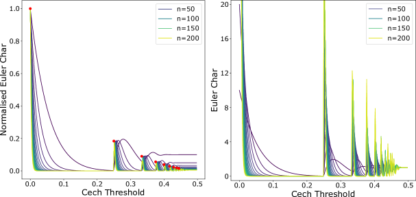
Figure 1. Left: Graphs of normalised expected Euler characteristics, $y=n^{-1}\cdot\bar{\chi}(n,x)$, for $n\in\{10,20,\ldots 200\}$ and $x\in[0,1]$. Right: Same as left, but we plot $y=\bar{\chi}(n,x)$, which are (un-normalised) expected Euler characteristics. Yellow curves correspond to larger $n$. Red circles are the limiting spikes, given by $\left(\frac{k}{2k+2},\frac{(k/e)^{k}}{(k+1)!}\right)$ for all $k\geq 0$.

Theorem A (Expected Euler Characteristic).

The following are true.
(1) $\bar{\chi}(n,r)$ is a continuous piecewise-polynomial function in $r$, given explicitly as follows for $n>0$ and $r\in(0,1)$: $$\bar{\chi}\left(n,\frac{1-r}{2}\right)=\sum_{k=1}^{\lfloor 1/r\rfloor}\binom{n}{k}(1-kr)^{k-1}(kr)^{n-k}$$ (2) Normalised Euler charactreristics have the following peak values for all $k\geq 0$: $\displaystyle\lim_{n\rightarrow\infty}\max_{r\in I_{k}}\frac{\bar{\chi}(n,r)}{n}=\frac{(k/e)^{k}}{(k+1)!}$ where $I_{k}=\left(\frac{k}{2k+2},\frac{k+1}{2k+4}\right)$. (3) Let $k\geq 1$. Given $\epsilon>0$, the following uniform bounds hold for all $r\in\left[\frac{k}{2k+2},\frac{k+1}{2k+4}\right)$ when $n$ is sufficiently large: $$\frac{\bar{\chi}(n,r)}{n}-\epsilon\leq\frac{\bar{b}_{2k}(n,r)}{n}\leq\frac{\bar{\chi}(n,r)}{n}$$

Theorem A allows us to plot exact values of the expected Euler characteristic curves. The left side of Figure 1 shows graphs of $f_{n}(r)=n^{-1}\cdot\bar{\chi}(n,r)$, which are normalised versions of $\bar{\chi}$. We stress that these curves are not empirically obtained from a method like Monte Carlo; they are plots of the formula in Theorem A1. As $n$ becomes larger, $f_{n}(r)$ shows peaks that converge to a sequence of narrow spikes, as Theorem A2 predicts. The right side of the same figure shows the non-normalised graphs of $\bar{\chi}(n,r)$, where we see that the limiting peaks of Theorem A2 will peak into infinity as $n\rightarrow\infty$.

Meanwhile all homotopy types arising from nerve complexes of circular arcs were completely classified in [4]: they are either $\mathbb{S}^{2k+1}$ for some $k\geq 0$, or $\vee^{a}\mathbb{S}^{2k}$ for some $a,k\geq 0$. We observe that $\chi(\mathbb{S}^{2k+1})=0$, whereas $\chi(\vee^{a}\mathbb{S}^{2k})=a+1$. Therefore in Figure 1, limiting spikes indicate contribution from the even-dimensional sphere bouquets $\vee^{a}\mathbb{S}^{2k}$ with large $a$, and the plateaus indicate contribution from the odd-dimensional spheres. Recalling that $\mathbf{X}_{n}$ is an i.i.d. sample of size $n$ drawn from $\mathbb{S}^{1}$, we have:

Theorem B (Odd Spheres).

Let $k\geq 0$ be an integer, and also let $\epsilon,\delta>0$. Suppose that $|r-\nu_{k}|\leq\tau_{k}-\epsilon$. Then for sufficiently large $n$, the following homotopy equivalence holds with probability at least $1-\delta$: $$\text{\v{C}}(\mathbf{X}_{n},r)\simeq\SS^{2k+1}$$ where $$\nu_{k}=\frac{2k^{2}+4k+1}{4(k+1)(k+2)},\quad\tau_{k}=\frac{1}{4(k+1)(k+2)}$$

Theorem C (Even Spheres).

Let $k\geq 2$, $\eta\in(0,1)$. Suppose that $|r-\rho_{k,n}|\leq\sigma_{k,\eta}/n$. Then for sufficiently large $n$, the following homotopy equivalence holds with probability at least $\eta\cdot k\omega_{k}$: $$\text{\v{C}}(\mathbf{X}_{n},r)\simeq\vee^{a}\mathbb{S}^{2k-2},\quad\text{for some }\frac{(1-\eta)\omega_{k}\cdot n}{2}\leq a+1\leq\frac{n}{k}$$ where $\displaystyle\rho_{k,n}=\frac{n(k+1)}{2k(n-1)},\quad\sigma_{k,\eta}=\frac{(1-\eta)^{3}(k\omega_{k})^{3}}{320\sqrt{k+2}},\quad\omega_{k}=\frac{(k-1)^{k-1}}{k!e^{k-1}}$

Remark 1. In Theorem B, we note that $\nu_{k}=\frac{1}{2}(\frac{k+1}{2k+4}+\frac{k}{2k+2})$ and $\tau_{k}=\frac{1}{2}(\frac{k+1}{2k+4}-\frac{k}{2k+2})$, so that Theorem B covers most of each interval $r\in[\frac{k}{2k+2},\frac{k+1}{2k+4}]$. Also to see Theorem C in action, one may simply set $\eta=1/2$ to obtain results.

Remark 2. Although all of the above results are proven for the Cech complex of circular arcs on the circle, similar behaviour are observed in the Rips complex constructed on the circle as well. Indeed, modifying Theorem B for the Rips complex immediately yields the following: for the Rips complex constructed from a finite random sample on a circle, all odd-dimensional spheres appear with positive persistence and probability approaching 1. Analogues of Theorems A and C for the Rips complex could not be immediately obtained with methods in this paper.

Structure of the paper. In Section 2 we prove Theorem A1, i.e. compute the expected Euler characteristic precisely. In Section 3 we prove Theorem A2 (Proposition 3.4), by analysing the limiting spikes of the expected Euler characteristics. In Section 4 we prove Theorem A3 and Theorem C, by using the classification of homotopy types arising from a nerve complex of circular arcs, thereby giving constraints on homotopy types and compute probabilistic bounds. In Section 5 we prove Theorem B, by using the classical method of stability of persistence diagram; this section works separately and doesn’t use the Euler characteristic method.

Theorem C takes the most work to prove. It is a simplified version of Theorem 4.8, which has a few more parameters that can be tweaked to obtain similar variants of Theorem C. Theorem 4.8 is obtained by combining three ingredients: Propositions 3.4, 4.5, and 4.7.

Related works.

The classical result of Hausmann shows that the Vietoris-Rips complex constructed from the manifold with a small scale parameter recovers the homotopy type of the manifold [12]. Another classical result of Niyogi, Smale, Weinberger shows that if a Cech complex of small filtration radius is constructed from a finite random sample of a Euclidean submanifold, then the homotopy type of the manifold is recovered with high confidence [15].

Much work has been done for recovering topology of a manifold from its finite sample, when connectivity radius is scaled down with the sample size at a specific rate [9] [11] [13] [10]. A central theme of this body of work is the existence of phase transitions when parameters controlling the scaling of connectivity radius are changed. For a comprehensive survey, see [17] and [8].

In comparison, the setting when connectivity radius is not scaled down with sample size is studied much less. Results on convergence of the topological quantities have been studied [16] [19], but not much attention has been devoted to analysing specific manifolds.

This paper builds on two important works that characterised the Vietoris-Rips and Cech complexes of subsets of the circle: [4] and [1]. Several variants of these ideas were studied, for ellipse [6], regular polygon [7], and hypercube graph [2]. Randomness in these systems were studied using dynamical systems in [5]. One key tool to further study the topology of Vietoris-Rips and Cech complexes arising from a manifold is metric thickening [3]. Using this tool, the Vietoris-Rips complex of the higher-dimensional sphere has been characterised up to small filtration radii [14].

Acknowledgements

The author is grateful to Henry Adams and Tadas Temčinas for valuable discussions that led up to this paper. The author would also like to thank Vidit Nanda and Harald Oberhauser for their contributions during initial stages of this research.
Uzu Lim is supported by the Korea Foundation for Advanced Studies.

2. Expected Euler characteristic

In this section we compute the expected Euler characteristic precisely. We start with a simple calculation that also briefly considers the Vietoris-Rips complex, but soon after we only work with the Cech complex. Let $\operatorname{VR}(\mathbf{X}_{n},r)$ denote the Vietoris-Rips complex of threshold $r$. The following proposition reduces computation of expected values to the quantities $T_{k}$ and $Q_{k}$, defined below:

Proposition 2.1.

For each $n>0$, let $\mathbf{X}_{n}$ be the iid sample drawn uniformly from $\mathbb{S}^{1}$. Then we have that:

$$\mathbb{E}[\chi(\operatorname{VR}(\mathbf{X}_{n},r))]= \sum_{k=1}^{n}(-1)^{k-1}\binom{n}{k}T_{k}(r)$$

$$\mathbb{E}[\chi(\text{\v{C}}(\mathbf{X}_{n},r))]= 1+\sum_{k=1}^{n}(-1)^{k}\binom{n}{k}Q_{k}(1-2r)$$

where $T_{k}(r)$ is the probability that every pair of points in $\mathbf{X}_{k}$ are within distance $r$, and $Q_{k}(r)$ is the probability that open arcs of length $r$ centered at points of $\mathbf{X}_{k}$ cover $\mathbb{S}^{1}$. Expectation is taken over the iid sample $\mathbf{X}_{n}$.

Proof.

Denoting by $s_{k}(K)$ the number of $k$-simplices in a simplicial complex $K$, we have that:

$$\mathbb{E}[s_{k}(\operatorname{VR}(\mathbf{X}_{n},r))]=\binom{n}{k}T_{k}(r)$$

and thus

$$\mathbb{E}[\chi(\operatorname{VR}(\mathbf{X}_{n},r))]=\sum_{k=0}^{n-1}(-1)^{k}\mathbb{E}[s_{k}(\operatorname{VR}(\mathbf{X}_{n},r))]=\sum_{k=1}^{n}(-1)^{k-1}\binom{n}{k}T_{k}(r)$$

The relation for the Cech complex is derived in the same way, except we note the following: the probability that arcs of radius $r$ centered at points of $\mathbf{X}_{k}$ intersects nontrivially is equal to $1-Q_{k}(1-2r)$. This is by De Morgan’s Law: for any collection of sets $\{U_{j}\subseteq\mathbb{S}^{1}\}_{j\in J}$, we have $\cap_{j\in J}U_{j}=\emptyset$ iff $\cup_{j\in J}U_{j}^{\operatorname{c}}=\mathbb{S}^{1}$. In the case of circle (of circumference 1), complement of a closed arc of radius $r$ is an open arc of length $1-2r$. Applying this logic, we obtain:

$$\mathbb{E}[\chi(\text{\v{C}}(\mathbf{X}_{n},r))]=\sum_{k=1}^{n}(-1)^{k-1}\binom{n}{k}(1-Q_{k}(1-2r))$$

which is easily seen to be the same as the asserted expression (note that $\sum_{k=1}^{n}(-1)^{k-1}\binom{n}{k}=1$.) ∎

The $Q_{k}$ were computed by Stevens in 1939 [18]. We reproduce the proof for completeness.

Theorem 2.2 (Stevens).

If $k$ arcs of fixed length $a$ are independently, identically and uniformly sampled from the circle of circumference 1, then the probability that these arcs cover the circle is equal to the following:

$$Q_{k}(a)=\sum_{l=0}^{\lfloor 1/a\rfloor}(-1)^{l}\binom{k}{l}(1-la)^{k-1}$$

Proof.

The proof is an application of inclusion-exclusion principle. Consider the set $E=\{(x_{1},\ldots x_{k})|0\leq x_{1}<\cdots<x_{k}<1\}$. For each collection of indices $J\subseteq\{1,\ldots k\}$, define $\bar{E}_{J}$ and $E_{J}$ as the following subsets of $E$:

$$E_{J}= \{(x_{1},\ldots x_{k})\in E|j\in J\iff x_{j+1}-x_{j}>a\}$$

$$\bar{E}_{J}= \{(x_{1},\ldots x_{k})\in E|j\in J\implies x_{j+1}-x_{j}>a\}=\bigsqcup_{J^{\prime}\supseteq J}E_{J^{\prime}}$$

By definition, we have $\operatorname{Vol}(E_{\emptyset})=Q_{k}(a)$. To compute it, we apply the inclusion-exclusion principle for the membership of each $E_{J}$ over $\bar{E}_{J^{\prime}}$ whenever $J^{\prime}\supseteq J$. Noting the relation $\sum_{l=1}^{k}(-1)^{l+1}\binom{k}{l}=1$, we see that:

$$1=\sum_{J\subseteq\{1,\ldots k\}}\operatorname{Vol}(E_{J})=\operatorname{Vol}(E_{\emptyset})-\sum_{\emptyset\neq J\subseteq\{1,\ldots k\}}(-1)^{\#J}\operatorname{Vol}(\bar{E}_{J})$$

Finally, if $l=\#J$ and $l\leq\lfloor 1/a\rfloor$, then $\operatorname{Vol}(\bar{E}_{J})=(1-la)^{n-1}$. This is because demanding gap conditions $x_{i+1}-x_{i}>a$ at $l$ places is equivalent to sampling $n-1$ points from an interval of length $1-la$. Meanwhile if $l>\lfloor 1/a\rfloor$, then we always have $\operatorname{Vol}(\bar{E}_{J})=0$. Plugging these into the above equation, we get:

$$\operatorname{Vol}(E_{\emptyset})=1+\sum_{l=1}^{\lfloor 1/a\rfloor}(-1)^{l}\binom{k}{l}(1-la)^{n-1}$$

as desired. ∎

We then get the following:

Theorem 2.3 (Theorem A).

Expected Euler characteristic of random Cech complex on a circle of unit circumference obtained from $n$ points and filtration radius $(1-r)/2$ is:

$$\bar{\chi}\left(n,\frac{1-r}{2}\right)=\sum_{k=1}^{\lfloor 1/r\rfloor}\binom{n}{k}(1-kr)^{k-1}(kr)^{n-k}$$

In particular, $\bar{\chi}(n,r)$ is a continuous piecewise-polynomial function in $r$.

Proof.

Substituting the $Q_{k}$ expression in, we get:

$$\bar{\chi}\left(n,\frac{1-r}{2}\right)= 1+\sum_{k=1}^{n}(-1)^{k}\binom{n}{k}Q_{k}(r)$$

$$= 1+\sum_{l=0}^{\lfloor 1/r\rfloor}\sum_{k=1}^{n}(-1)^{k+l}\binom{n}{k}\binom{k}{l}(1-rl)^{k-1}$$

$$= \sum_{l=1}^{\lfloor 1/r\rfloor}\sum_{k=1}^{n}(-1)^{k+l}\binom{n}{k}\binom{k}{l}(1-rl)^{k-1}$$

where we switched the order of summation in the second equality, and isolating the $l=0$ part cancels out the $1$ in the third equality. Noting that $\binom{n}{k}\binom{k}{l}=\binom{n}{l}\binom{n-l}{k-l}$, we further get:

$$\bar{\chi}\left(n,\frac{1-r}{2}\right)= \sum_{l=1}^{\lfloor 1/r\rfloor}(-1)^{l}\binom{n}{l}(1-rl)^{-1}\sum_{k=l}^{n}\binom{n-l}{k-l}(rl-1)^{k}$$

$$= \sum_{l=1}^{\lfloor 1/r\rfloor}\binom{n}{l}(1-rl)^{l-1}\sum_{k=0}^{n-l}\binom{n-l}{k}(rl-1)^{k}$$

$$= \sum_{l=1}^{\lfloor 1/r\rfloor}\binom{n}{l}(1-rl)^{l-1}(rl)^{n-l}$$

∎

3. Limit behaviour of Euler characteristic

We prove a sequence of lemmas in this section to characterise the limiting spikes in Figure 1. The main idea is that only one summand in the expected Euler characteristic contributes mainly to the spike, and this is a polynomial term that can be studied with calculus. The main results of this section are Propositions 3.3 and 3.4. The two lemmas leading up to it are exercises in calculus that explain the specific situation of our expected Euler characteristic.

Lemma 3.1.

For $a,b\geq 1$, the function $f(t)=t^{a}(1-t)^{b}$ satisfies the following:

(a) In the range $0\leq t\leq 1$, $f(t)$ achieves the unique maximum value at $t=a/(a+b)$:

$$\max_{0\leq t\leq 1}f(t)=f\left(\frac{a}{a+b}\right)=\frac{a^{a}b^{b}}{(a+b)^{a+b}}$$

Also, $f(t)$ is increasing on $t\in(0,a/(a+b))$ and decreasing on $t\in(a/(a+b),1)$.

(b) The following linear lower bounds hold:

$$f(t)\geq u\bigg{(}(a+b)vt-av+1\bigg{)}\text{, when }0<t<\frac{a}{a+b}$$

$$f(t)\geq u\bigg{(}-(a+b)vt+av+1\bigg{)}\text{, when }\frac{a}{a+b}<t<1$$

where

$$u=\frac{a^{a}b^{b}}{(a+b)^{a+b}},\quad v=\sqrt{\frac{a+b}{ab}}$$

(c) For each $\lambda\in[0,1]$, we have that:

$$\left|t-\frac{a}{a+b}\right|<\frac{(1-\lambda)\sqrt{ab}}{(a+b)^{3/2}}\implies t^{a}(1-t)^{b}>\lambda u$$

Proof.

The first two derivatives are:

$$f^{\prime}(t)= \bigg{(}a-(a+b)t\bigg{)}t^{a-1}(1-t)^{b-1}$$

$$f^{\prime\prime}(t)= \bigg{(}(a+b)(a+b-1)t^{2}+2a(1-a-b)t+a(a-1)\bigg{)}t^{a-2}(1-t)^{b-2}$$

The first derivative vanishes at $t\in\{a/(a+b),0,1\}$ and the second derivative vanishes at $t\in\{t_{0}\pm\eta_{0},0,1\}$ where

$$t_{0}=\frac{a}{a+b},\quad\eta_{0}=\frac{1}{a+b}\sqrt{\frac{ab}{a+b-1}}>\frac{\sqrt{ab}}{(a+b)^{3/2}}=\eta_{1}$$

The first derivative is positive at $(0,a/(a+b))$ and negative at $(a/(a+b),1)$. Thus the maximum at $t\in[0,1]$ is given by:

$$f(t_{0})=\frac{a^{a}b^{b}}{(a+b)^{a+b}}$$

Thus

$$f(t)\geq\frac{f(t_{0})}{\eta_{1}}(t-t_{0})+f(t_{0})\text{, when }0<t<t_{0}$$

$$f(t)\geq\frac{-f(t_{0})}{\eta_{1}}(t-t_{0})+f(t_{0})\text{, when }t_{0}<t<1$$

and

$$\pm\frac{f(t_{0})}{\eta_{1}}(t-t_{0})+f(t_{0})= \frac{a^{a}b^{b}}{(a+b)^{a+b}}\left(\pm\frac{(a+b)^{3/2}}{\sqrt{ab}}\left(t-\frac{a}{a+b}\right)+1\right)$$

(c) follows from the linear bound of (b). ∎

Lemma 3.2.

Let $m,n\geq 1$ be integers and define:

$$f_{m,n}(t)=\binom{n}{m}(mt)^{m-1}(1-mt)^{n-m}$$

Then $f_{m,n}$ satisfies the following:

(a) $f_{m,n}(t)$ is increasing when $0<t<t_{0}$ and decreasing when $t_{0}<t<1/m$ where $t_{0}=\frac{1}{n-1}(1-\frac{1}{m})$.

(b) The maximum over $0<t<1/m$ is given by:

$$\max_{0<mt<1}f_{m,n}(t)=f_{m,n}(t_{0})=\binom{n}{m}\frac{(m-1)^{m-1}(n-m)^{n-m}}{(n-1)^{n-1}}$$

(c) For each $\lambda\in[0,1]$, we have that:

$$|t-t_{0}|<\frac{(1-\lambda)\sqrt{(m-1)(n-m)}}{m(n-1)^{3/2}}\implies f_{m,n}(t)>\lambda f_{m,n}(t_{0})$$

(d) The normalised limit of maximum as $n\rightarrow\infty$ is given by:

$$\lim_{n\rightarrow\infty}\frac{\max_{0<t<1/m}f_{m,n}(t)}{n}=\frac{(m-1)^{m-1}}{m!e^{m-1}}$$

Proof.

(a)-(c) follow from the previous lemma. For (d), we compute:

$$\lim_{n\rightarrow\infty}\frac{\max_{0<t<1/m}f_{m,n}(t)}{n}= \frac{(m-1)^{m-1}}{m!}\lim_{n\rightarrow\infty}(n-1)(n-2)\cdots(n-m+1)\frac{(n-m)^{n-m}}{(n-1)^{n-1}}$$

$$= \frac{(m-1)^{m-1}}{m!}\lim_{n\rightarrow\infty}\frac{(n-m)^{n-m}}{(n-1)^{n-m}}$$

and also

$$\lim_{n\rightarrow\infty}\frac{(n-m)^{n-m}}{(n-1)^{n-m}}=\lim_{n\rightarrow\infty}\left(1-\frac{m-1}{n-1}\right)^{n-m}=\lim_{n\rightarrow\infty}\left(1-\frac{m-1}{n-1}\right)^{n-1}=\frac{1}{e^{m-1}}$$

which gives the desired expression. ∎

Proposition 3.3.

Suppose that $m,n$ are integers with $2\leq m<\sqrt{n}$. The following holds for $\bar{\chi}(n,r)$.

(a) The following bounds hold:

$$a_{m,n}\leq\frac{\bar{\chi}(n,s_{m,n})}{n}\leq M\leq a_{m,n}+b_{m,n}$$

where

$$M= \max\left\{\frac{1}{n}\bar{\chi}\left(n,\frac{1-r}{2}\right)\>\bigg{|}\>r\in\left(\frac{1}{m+1},\frac{1}{m}\right)\right\}$$

$$s_{m,n}= \frac{(m-1)n}{2(n-1)m}$$

$$a_{m,n}= \binom{n}{m}\frac{(m-1)^{m-1}(n-m)^{n-m}}{n(n-1)^{n-1}}$$

$$b_{m,n}= en^{m-1}\left(1-\frac{1}{m+1}\right)^{n-1}$$

(b) We have the following limits:

$$\lim_{n\rightarrow\infty}a_{m,n}=\frac{(m-1)^{m-1}}{m!e^{m-1}},\quad\lim_{n\rightarrow\infty}b_{m,n}=0$$

(c) Suppose additionally that $n>2m^{2}$. Then for each $\lambda\in[0,1]$, we have that:

$$\left|r-\frac{n-m}{(n-1)m}\right|<\frac{(1-\lambda)\sqrt{(m-1)(n-m)}}{m(n-1)^{3/2}}\implies\frac{1}{n}\bar{\chi}\left(n,\frac{1-r}{2}\right)>\lambda a_{m,n}$$

This condition for $r$ in particular satisfies $r\in\left(\frac{1}{m+1},\frac{1}{m}\right]$.

Proof.

Let $r\in\left(\frac{1}{m+1},\frac{1}{m}\right]$ and also write $r=\frac{1}{m}-t$, with $t\in\left[0,\frac{1}{m(m+1)}\right]$. Then we may rewrite the normalised expected Euler characteristic as follows:

$$\bar{\chi}\left(n,\frac{1-r}{2}\right)= \sum_{k=1}^{m}\binom{n}{k}(1-kr)^{k-1}(kr)^{n-k}$$

$$= \sum_{k=1}^{m}\binom{n}{k}\left(1-\frac{k}{m}+kt\right)^{k-1}\left(\frac{k}{m}-kt\right)^{n-k}$$

We now claim that the $k=m$ term is the dominant one among the above summands. As such, we split the above sum as:

$$\bar{\chi}\left(n,\frac{1-r}{2}\right)=f_{m,n}(t)+E$$

where

$$f_{m,n}(t)= \binom{n}{m}(mt)^{m-1}(1-mt)^{n-m},$$

$$E= \sum_{k=1}^{m-1}\binom{n}{k}\left(1-\frac{k}{m}+kt\right)^{k-1}\left(\frac{k}{m}-kt\right)^{n-k}$$

Since $m<\sqrt{n}$, we have $s_{m,n}=\frac{1}{n-1}(1-\frac{1}{m})<\frac{1}{m(m+1)}$. Therefore, the previous Lemma tells us that $f_{m,n}(t)$ achieves (global) maximum at $\tilde{s}\in\left(0,\frac{1}{m(m+1)}\right]$, with the maximum value given by:

$$f_{m,n}(\tilde{s})=n\cdot a_{m,n}\text{, where }a_{m,n}=\binom{n}{m}\frac{(m-1)^{m-1}(n-m)^{n-m}}{n(n-1)^{n-1}}$$

We also bound $E$ as follows, using the inequality $\frac{m}{m+1}<1-mt\leq 1$:

$$E= \sum_{k=1}^{m-1}\binom{n}{k}\left(1-\frac{k}{m}(1-mt)\right)^{k-1}\left(\frac{k}{m}(1-mt)\right)^{n-k}$$

$$\leq \sum_{k=1}^{m-1}\binom{n}{k}\left(1-\frac{1}{m+1}\right)^{k-1}\left(1-\frac{1}{m}\right)^{n-k}$$

$$\leq \sum_{k=1}^{m-1}\frac{n^{k}}{k!}\left(1-\frac{1}{m+1}\right)^{n-1}$$

$$\leq en^{m-1}\left(1-\frac{1}{m+1}\right)^{n-1}$$

This shows (a). Now (b) follows from the previous Lemma and the fact that $(1-\frac{1}{m+1})^{n}$ term causes exponential decay for $b_{m,n}$.

(c) follows from (c) of the previous Lemma. We additionally impose the condition $n>2m^{2}$, so that the endpoints of $t$ satisfying the condition fall in the interval $t\in\left[0,\frac{1}{m(m+1)}\right)$. ∎

The following yields Theorem A2.

Proposition 3.4.

Let $m\geq 2$, $\epsilon>0$. The following holds for sufficiently large $n$:

$$r\in\left[\alpha^{-},\alpha^{+}\right]\implies\frac{1}{n}\bar{\chi}\left(n,\frac{1-r}{2}\right)\in\bigg{[}(1-\epsilon)\omega_{m},(1+\epsilon)\omega_{m}\bigg{]}$$

where

$$\alpha^{\pm}= \frac{n-m}{(n-1)m}\left(1\pm\frac{\epsilon\sqrt{m-1}}{n}\right),\quad\omega_{m}=\frac{(m-1)^{m-1}}{m!e^{m-1}}$$

Proof.

This follows directly from the previous Proposition. $\alpha^{\pm}$ are slight relaxations of the interval in (c), where we set $\lambda=1-\epsilon$:

$$\left[\frac{n-m}{(n-1)m}-\epsilon R_{1},\frac{n-m}{(n-1)m}+\epsilon R_{1}\right]\supseteq\left[\frac{n-m}{(n-1)m}(1-\epsilon R_{2}),\frac{n-m}{(n-1)m}(1+\epsilon R_{2})\right]$$

$$\text{where }R_{1}=\frac{\epsilon\sqrt{(m-1)(n-m)}}{m(n-1)^{3/2}},\quad R_{2}=\frac{\sqrt{m-1}}{n}$$

∎

4. Random homotopy types

4.1. Constraints on homotopy types

Let $\mathbf{U}_{n}=\{i/n\>|\>i=0,1,\ldots n-1\}\subset{\mathbb{S}^{1}}$ be the set of $n$ equally spaced points. Let $\mathcal{N}(n,k)$ be the nerve complex on $\mathbf{U}_{n}$ defined by the open cover consisting of closed intervals $[i/n,(i+k)/n]$.

Lemma 4.1.

We have that:

$$\text{\v{C}}(\mathbf{U}_{n},r)=\text{\v{C}}\bigg{(}\mathbf{U}_{n},\frac{\lfloor 2rn\rfloor}{2n}\bigg{)}=\mathcal{N}(n,\lfloor 2rn\rfloor)$$

The following result is from [4]:

Proposition 4.2.

$$\mathcal{N}(n,k)\simeq\begin{cases}\vee^{n-k-1}\mathbb{S}^{2l}&\text{if }\frac{k}{n}=\frac{l}{l+1}\\ \mathbb{S}^{2l+1}&\text{if }\frac{k}{n}\in\left(\frac{l}{l+1},\frac{l+1}{l+2}\right)\end{cases}$$

Note that if $(k,n)=(jl,j(l+1))$, then $n-k-1=j-1$, so that $\vee^{n-k-1}\mathbb{S}^{2l}=\vee^{j-1}\mathbb{S}^{2l}$.

Using the above, we easily show that:

Proposition 4.3.

Given $r\in(0,1/2)$, the following two subsets of $\mathbb{Z}^{3}$ are equal:

$$\bigg{\{}(n,a,b)\>\bigg{|}\>\text{\v{C}}(\mathbf{U}_{n},r)\simeq\vee^{a}\mathbb{S}^{2b}\bigg{\}}=\bigg{\{}((a+1)(b+1),a,b)\>\bigg{|}\>b+1\leq\tilde{r}^{-1},\>a+1\leq\frac{1}{1-(b+1)\tilde{r}}\bigg{\}}$$

where $\tilde{r}=1-2r$. In particular, if $\tilde{r}^{-1}\in[k,k+1)$, then $b\in\{0,1,2,\ldots k-1\}$ and we have $a\leq k-1$ when $b\leq k-2$.

Proof.

To have $\mathcal{N}(n,\lfloor 2rn\rfloor)=\text{\v{C}}(\mathbf{U}_{n},r)\simeq\vee^{a}\mathbb{S}^{2b}$, we see from the previous Proposition that the condition is given by $(\lfloor 2rn\rfloor,n)=((a+1)b,(a+1)(b+1))$. This determines $n$ from $(a,b)$. The condition on $\lfloor 2rn\rfloor$ is then:

$$(a+1)b\leq 2r(a+1)(b+1)<(a+1)b+1$$

$$\iff \tilde{r}(b+1)\leq 1,\>a<\tilde{r}(a+1)(b+1)$$

$$\iff (b+1)\leq\tilde{r}^{-1},\>(a+1)<(1-\tilde{r}(b+1))^{-1}$$

as desired. ∎

Remark. At fixed $l$, let $k=b+k_{0}$. Then $\frac{1}{1-(b+1)/k}=1+\frac{b+1}{k_{0}-1}$ and changing $k_{0}$ by a single value can have a heavy effect on the upper bound.

Proposition 4.4.

Let $r\in(0,1/2)$ and $n$ be given; define $\tilde{r}=1-2r$ and let $k=\lfloor\tilde{r}^{-1}\rfloor$. We have the following relations between subsets of $\mathbb{Z}^{2}$:

$$\bigg{\{}(a,b)\>\bigg{|}\>\text{\v{C}}(\mathbf{Y},r)\simeq\vee^{a}\mathbb{S}^{2b},\>\mathbf{Y}\subset\mathbb{S}^{1},\>\#\mathbf{Y}=n\bigg{\}}$$

$$= \bigg{\{}(a,b)\>\bigg{|}\>\text{\v{C}}(\mathbf{U}_{m},r)\simeq\vee^{a}\mathbb{S}^{2b},\>m\leq n\bigg{\}}$$

$$\subseteq \bigg{\{}(a,b)\>\bigg{|}\>b+1\leq k,\>a+1\leq\min\bigg{(}\frac{n}{b+1},\frac{1}{1-(b+1)\tilde{r}}\bigg{)}\bigg{\}}$$

$$\subseteq \bigg{\{}(a,b)\>\bigg{|}\>b+1\leq k-1,\>a+1\leq\frac{k}{k-b-1}\bigg{\}}\cup\bigg{\{}(a,k-1)\>\bigg{|}\>a+1\leq\frac{n}{k}\bigg{\}}$$

where in the final expression, $k/0=\infty$ by convention.

Proof.

The first equality holds because for every $\mathbf{Y}\subset\mathbb{S}^{1}$, there exists $\mathbf{Y}^{\prime}\subset\mathbf{Y}$ such that $\text{\v{C}}(\mathbf{Y},r)\simeq\text{\v{C}}(\mathbf{Y}^{\prime},r)\simeq\text{\v{C}}(\mathbf{U}_{m},r)$, where $m=\#\mathbf{Y}^{\prime}$ [4]. The first inclusion follows from the previous Proposition. The second inclusion follows from separating the two cases $b+1<k$ and $b+1=k$. ∎

4.2. Probabilistic bounds

For a topological space $K$, we define the following notation for probability:

$$p(K,n,r)=\mathbb{P}[\text{\v{C}}(\mathbf{X}_{n},r)\simeq K]$$

We generally have the following:

$$\bar{\chi}(n,r)=\mathbb{E}[\chi(\text{\v{C}}(\mathbf{X}_{n},r))]=\sum_{K}\chi(K)\cdot p(K,n,r)$$

where the sum is well-defined because there are only finitely many combinatorial structures that $\text{\v{C}}(\mathbf{X}_{n},r)$ can take. Furthermore if we let $k=\lfloor(1-2r)^{-1}\rfloor$, then Proposition 4.4 tells us that:

$$\{K\>|\>p(K,n,r)>0\}\subseteq\bigg{\{}\vee^{a}\mathbb{S}^{2b}\>\bigg{|}\>b+1\leq k-1,a+1\leq\frac{k}{k-b-1}\bigg{\}}\cup\bigg{\{}\vee^{a}\mathbb{S}^{2k-2}\>\bigg{|}\>a+1\leq\frac{n}{k}\bigg{\}}$$

From this we infer that:

$$\bar{\chi}(n,r)= A_{<k}+A_{k}$$

$$\text{where }A_{<k}= \sum_{\begin{subarray}{c}0\leq b\leq k-2\\ (a+1)(k-b-1)\leq k\end{subarray}}(a+1)\cdot p(\vee^{a}\mathbb{S}^{2b},n,r)$$

$$A_{k}= \sum_{1<a+1\leq n/k}(a+1)\cdot p(\vee^{a}\mathbb{S}^{2k-2},n,r)$$

where we used $\chi(\vee^{a}\mathbb{S}^{2b})=a+1$. Since sum of probabilities is $1$, applying the constraint $(a+1)(k-b-1)\leq k$ implies that $A_{<k}\leq k$. This implies the following:

Proposition 4.5.

The following holds:

$$A_{k}\leq\bar{\chi}(n,r)\leq k+A_{k}$$

where

$$A_{k}=\sum_{1<a+1\leq n/k}(a+1)\cdot p(\vee^{a}\mathbb{S}^{2k-2},n,r)$$

Corollary 4.6 (Theorem A3).

Let $k\geq 2$. Given $\epsilon>0$, the following hold for sufficiently large $n$:

$$1-2r\in\left(\frac{1}{k+1},\frac{1}{k}\right]\implies\frac{\bar{\chi}(n,r)}{n}-\epsilon\leq\frac{\bar{b}_{2k-2}(n,r)}{n}\leq\frac{\bar{\chi}(n,r)}{n}$$

Now we’re interested in controlling probabilities that $\vee^{a}\mathbb{S}^{2k-2}$ appear, with large $n$. For this, we further define following:

$$p_{a}= p(\vee^{a}\mathbb{S}^{2k-2},n,r)$$

$$l= \lfloor n/k\rfloor-1$$

$$\tilde{\delta}= \lceil\delta n/k\rceil-1$$

$$A_{k,\delta}:= \sum_{\tilde{\delta}\leq a\leq l}(a+1)\cdot p_{a}=\sum_{\delta n/k\leq a+1\leq n/k}(a+1)\cdot p_{a}$$

$$B_{k,\delta}:= \sum_{\tilde{\delta}\leq a\leq l}p_{a}$$

To produce bounds for $B_{k,\delta}$, we split $A_{k}$ into two parts:

$$A_{k}=\bigg{(}2p_{1}+3p_{2}+\cdots+\tilde{\delta}p_{\tilde{\delta}-1}\bigg{)}+\bigg{(}(\tilde{\delta}+1)p_{\tilde{\delta}}+\cdots+(l+1)p_{l}\bigg{)}$$

from which it directly follows that:

$$(\tilde{\delta}+1)B_{k,\delta}\leq A_{k}\leq\tilde{\delta}(1-B_{k,\delta})+(l+1)B_{k,\delta}$$

and therefore

$$\implies (\tilde{\delta}+1)B_{k,\delta}\leq A_{k}\leq\tilde{\delta}+(l+1-\tilde{\delta})B_{k,\delta}$$

$$\implies \frac{A_{k}-\tilde{\delta}}{l+1-\tilde{\delta}}\leq B_{k,\delta}\leq\frac{A_{k}}{\tilde{\delta}+1}$$

$$\implies \frac{A_{k}-\lceil\delta n/k\rceil+1}{\lfloor n/k\rfloor-\lceil\delta n/k\rceil+1}\leq B_{k,\delta}\leq\frac{A_{k}}{\lceil\delta n/k\rceil}$$

$$\implies \frac{A_{k}-\delta n/k}{(1-\delta)(n/k)+1}\leq B_{k,\delta}\leq\frac{A_{k}}{\delta n/k}$$

In summary, we have the following:

Proposition 4.7.

Let $n\in\mathbb{Z}^{+}$, $\delta\in(0,1)$, $r\in(0,1/2)$ be given, and let $k=\lfloor(1-2r)^{-1}\rfloor$. The following holds:

$$\frac{kA_{k}-\delta n}{(1-\delta)n+k}\leq B_{k,\delta}\leq\frac{kA_{k}}{\delta n}$$

where

$$A_{k}= \sum_{1<a+1\leq n/k}(a+1)p_{a},\quad B_{k,\delta}:=\sum_{\delta n/k\leq a+1\leq n/k}p_{a},\quad p_{a}:=p(\vee^{a}\mathbb{S}^{2k-2},n,r)$$

Now Propositions 3.4, 4.5, 4.7 imply the following, which is a more general version of Theorem C:

Theorem 4.8.

Let $r\in[\frac{1}{4},\frac{1}{2})$ and let $k=\lfloor(1-2r)^{-1}\rfloor$. Given $\epsilon,\delta\in(0,1)$, the following implication holds for large enough $n$:

$$1-2r\in[\alpha^{-},\alpha^{+}]\implies B_{k,\delta}\in[\beta^{-}-\epsilon,\beta^{+}+\epsilon]$$

where

$$\alpha^{\pm}= \frac{1}{k}\frac{n-k}{n-1}\bigg{(}1\pm\frac{\sqrt{k-1}}{n}\cdot\frac{\delta(1-\delta)}{5}\cdot\epsilon\bigg{)},$$

$$\beta^{-}= \frac{k\omega_{k}-\delta}{1-\delta},\quad\beta^{+}=\frac{k\omega_{k}}{\delta}$$

$$\omega_{k}= \frac{(k-1)^{k-1}}{k!e^{k-1}}$$

$$B_{k,\delta}:= \sum_{\delta n/k\leq a+1\leq n/k}p(\vee^{a}\mathbb{S}^{2k-2},n,r)$$

The bounds $\beta^{\pm}$ satisfy $\beta^{-}\leq k\omega_{k}\leq\beta^{+}$. Also $\beta^{-}>0$ iff $\delta<k\omega_{k}$ and $\beta^{+}<1$ iff $\delta>k\omega_{k}$.

Proof.

We first describe the heuristic reasoning for the bounds, which is rather simple. Proposition 4.7 gives us:

$$\frac{kA_{k}-\delta n}{(1-\delta)n+k}\leq B\leq\frac{kA_{k}}{\delta n}$$

By Proposition 3.4 and 4.5, the upper bound has the following approximations:

$$\frac{kA_{k}}{\delta n}\approx\frac{k\bar{\chi}}{\delta n}\approx\frac{k\omega_{k}}{\delta}$$

and similarly the lower bound has the following approximations:

$$\frac{kA_{k}-\delta n}{(1-\delta)n+k}\approx\frac{kA_{k}-\delta n}{(1-\delta)n}\approx\frac{k\bar{\chi}-\delta}{1-\delta}\approx\frac{k\omega_{k}-\delta}{1-\delta}$$

The actual proof becomes more complicated due to using a different choice of $\epsilon$ in applying Proposition 3.4.

Let $\epsilon^{\prime}=\delta(1-\delta)\cdot\epsilon/5$. We apply Proposition 3.4 with $\epsilon^{\prime}$ taking the role of $\epsilon$, and this gives the choice of $\alpha^{\pm}$ in the theorem. Therefore $r\in[\alpha^{-},\alpha^{+}]$ implies the following:

(4.1) $$(1-\epsilon^{\prime})\omega_{k}\leq\frac{\bar{\chi}}{n}\leq(1+\epsilon^{\prime})\omega_{k}$$

Before going further, we note the following inequalities for $\epsilon^{\prime}$, which we will use later:

$$\epsilon^{\prime}=\frac{\delta(1-\delta)\epsilon}{4+1}\leq\frac{\delta(1-\delta)\epsilon}{4+\delta(1-\delta)\epsilon}$$

$$\implies \frac{\epsilon^{\prime}}{1-\epsilon^{\prime}}\leq\frac{\delta(1-\delta)\epsilon}{4}$$

(4.2) $$\implies \frac{\epsilon^{\prime}}{1-\epsilon^{\prime}}\leq\min\bigg{(}4\delta,\delta^{-1}-1,1\bigg{)}\cdot\frac{\epsilon}{4}$$

Upper bound.

By Equation (4.1) and Proposition 4.5, we have:

$$\frac{k\omega_{k}}{\delta}\geq\frac{1}{1+\epsilon^{\prime}}\frac{k\bar{\chi}}{\delta n}\geq\frac{1}{1+\epsilon^{\prime}}\frac{kA_{k}}{\delta n}$$

By Equation (4.2), we have that:

$$\frac{1}{1+\epsilon^{\prime}}\frac{kA_{k}}{\delta n}\geq\frac{kA_{k}}{\delta n}-\epsilon$$

Then Proposition 4.7 applies and we have the upper bound.

Lower bound.

By Equation (4.1) and Proposition 4.5, we have:

$$\frac{k\omega_{k}-\delta}{1-\delta}\leq\frac{1}{1-\delta}\bigg{(}\frac{1}{1-\epsilon^{\prime}}\frac{k\bar{\chi}}{n}-\delta\bigg{)}\leq\frac{1}{1-\delta}\bigg{(}\frac{1}{1-\epsilon^{\prime}}\frac{k^{2}+kA_{k}}{n}-\delta\bigg{)}$$

Let $L_{0}$ be the right hand side. We rewrite it as follows:

$$L_{0}=L_{1}+E_{1}=L_{2}+E_{1}+E_{2}$$

where

$$L_{1}= \frac{kA_{k}-\delta n}{(1-\delta)(1-\epsilon^{\prime})n},\>E_{1}=\frac{\delta\epsilon^{\prime}+k^{2}/n}{(1-\delta)(1-\epsilon^{\prime})}$$

$$L_{2}= \frac{kA_{k}-\delta n}{(1-\delta)n+k},\>E_{2}=\frac{kA_{k}-\delta n}{(1-\delta)(1-\epsilon^{\prime})n}\cdot\frac{k+(1-\delta)n\epsilon^{\prime}}{(1-\delta)n+k}$$

By Equation (4.2), the relation $kA_{k}\leq n$ and by taking $n$ large enough, we see that

$$E_{1},E_{2}\leq\epsilon/2$$

This implies that:

$$\frac{k\omega_{k}-\delta}{1-\delta}-\epsilon\leq L_{0}-\epsilon=L_{2}+E_{1}+E_{2}-\epsilon\leq L_{2}$$

Then again Proposition 4.7 applies and we have the lower bound.

∎

We remark that Theorem C is obtained by setting $\epsilon=\delta=(1-\alpha)k\omega_{k}/2$. The gap $\alpha^{+}-\alpha^{-}$ is replaced by a smaller but simpler quantity.

5. Odd spheres

We prove Theorem B using the stability of persistence diagram. In this case, we will be using the Cech complex constructed from the full set of the circle, and then bound the Gromov-Hausdorff distance between the full circle and a finite sample of it. We use the following result from [1]:

Theorem 5.1.

The homotopy types of the Rips and Cech complexes on the circle of unit circumference are as follows:

$$\operatorname{VR}(\SS^{1},r) \simeq\begin{cases}\SS^{2l+1}&\text{,if }\frac{l}{2l+1}<r<\frac{l+1}{2l+3}\\ \bigvee^{\mathfrak{c}}\SS^{2l}&\text{,if }r=\frac{l}{2l+1}\end{cases}$$

$$\text{\v{C}}(\SS^{1},r) \simeq\begin{cases}\SS^{2l+1}&\text{,if }\frac{l}{2l+2}<r<\frac{l+1}{2l+4}\\ \bigvee^{\mathfrak{c}}\SS^{2l}&\text{,if }r=\frac{l}{2l+2}\end{cases}$$

where $\mathfrak{c}$ is the cardinality of the continuum.

We also note the stability of persistence:

Theorem 5.2 (Stability of Persistence).

If $X,Y$ are metric spaces and $\mathcal{D}_{k}M$ is the $k$-dimensional persistence diagram of persistence module $M$, then

$$\operatorname{d}_{B}(\mathcal{D}_{k}\mathbf{VR}(X),\mathcal{D}_{k}\mathbf{VR}(Y)) \leq\operatorname{d}_{GH}(X,Y)$$

$$\operatorname{d}_{B}(\mathcal{D}_{k}\text{\v{C}}(X),\mathcal{D}_{k}\text{\v{C}}(Y)) \leq\operatorname{d}_{GH}(X,Y)$$

where $\operatorname{d}_{GH}$ denotes the Gromov-Hausdorff distance.

The following proposition is a more precise version of Theorem B, which specifies an explicit lower bound for the probabilities of homotopy equivalence:

Proposition 5.3.

For each $l\geq 0$ and $t\in(\frac{l}{2l+2},\frac{l+1}{2l+4})$, the following holds with probability at least $Q_{n}(r^{\prime}/2)$:

$$\text{\v{C}}(\mathbf{X}_{n},t)\simeq\SS^{2l+1}$$

where $r^{\prime}$ is:

$$r^{\prime}=\frac{1}{4(l+1)(l+2)}-\left|t-\frac{2l^{2}+4l+1}{4(l+1)(l+2)}\right|$$

Proof.

Consider a random sample $\mathbf{X}_{n}=(X_{1},\ldots X_{n})$. Then with probability $Q_{n}(r/2)$, arcs of radius $r$ centered at $\mathbf{X}_{n}$ covers $\SS^{1}$, so that $\operatorname{d}_{GH}(\mathbf{X}_{n},\SS^{1})\leq\operatorname{d}_{H}(\mathbf{X}_{n},\SS^{1})\leq r$. This implies:

$$\operatorname{d}_{B}(\mathcal{D}_{k}\text{\v{C}}(\mathbf{X}_{n}),\mathcal{D}_{k}\text{\v{C}}(\SS^{1}))\leq\operatorname{d}_{GH}(\mathbf{X}_{n},\SS^{1})\leq r$$

For each $l\geq 0$, we have that:

$$\mathcal{D}_{2l+1}\text{\v{C}}(\SS^{1})=\left\{\left(\frac{l}{2l+2},\frac{l+1}{2l+4}\right)\right\}$$

so that the definition of the bottleneck distance implies that

$$\exists(u,v)\in\mathcal{D}_{2l+1}\text{\v{C}}(\mathbf{X}_{n})$$

with $$\frac{l}{2l+2}-r\leq u\leq\frac{l}{2l+2}+r$$

$$\frac{l+1}{2l+4}-r\leq v\leq\frac{l+1}{2l+4}+r$$

This implies that whenever $\frac{l}{2l+2}+r\leq t\leq\frac{l+1}{2l+4}-r$, we have:

$$1\leq\dim H_{2l+1}\text{\v{C}}(\mathbf{X}_{n},t)$$

and due to the enumeration of possible homotopy types, we have that:

$$\text{\v{C}}(\mathbf{X}_{n},t)\simeq\SS^{2l+1}$$

The condition translates to $\left|t-\frac{1}{2}\left(\frac{l}{2l+2}+\frac{l+1}{2l+4}\right)\right|<\frac{1}{2}\left(\frac{l+1}{2l+4}-\frac{l}{2l+2}\right)-r$, or equivalently

$$\left|t-\frac{2l^{2}+4l+1}{4(l+1)(l+2)}\right|<\frac{1}{4(l+1)(l+2)}-r$$

and thus we obtain the proof.

∎

References

• [1] M.ย Adamaszek and H.ย Adams. The vietorisโ€“rips complexes of a circle. Pacific Journal of Mathematics, 290(1):1โ€“40, 2017.
• [2] M.ย Adamaszek and H.ย Adams. On vietorisโ€“rips complexes of hypercube graphs. Journal of Applied and Computational Topology, 6(2):177โ€“192, 2022.
• [3] M.ย Adamaszek, H.ย Adams, and F.ย Frick. Metric reconstruction via optimal transport. SIAM Journal on Applied Algebra and Geometry, 2(4):597โ€“619, 2018.
• [4] M.ย Adamaszek, H.ย Adams, F.ย Frick, C.ย Peterson, and C.ย Previte-Johnson. Nerve complexes of circular arcs. Discrete & Computational Geometry, 56:251โ€“273, 2016.
• [5] M.ย Adamaszek, H.ย Adams, and F.ย Motta. Random cyclic dynamical systems. Advances in Applied Mathematics, 83:1โ€“23, 2017.
• [6] M.ย Adamaszek, H.ย Adams, and S.ย Reddy. On vietorisโ€“rips complexes of ellipses. Journal of Topology and Analysis, 11(03):661โ€“690, 2019.
• [7] H.ย Adams, S.ย Chowdhury, A.ย Q. Jaffe, and B.ย Sibanda. Vietoris-rips complexes of regular polygons. arXiv preprint arXiv:1807.10971, 2018.
• [8] O.ย Bobrowski and M.ย Kahle. Topology of random geometric complexes: a survey. Journal of applied and Computational Topology, 1:331โ€“364, 2018.
• [9] O.ย Bobrowski and G.ย Oliveira. Random ฤech complexes on riemannian manifolds. Random Structures & Algorithms, 54(3):373โ€“412, 2019.
• [10] O.ย Bobrowski and S.ย Weinberger. On the vanishing of homology in random ฤech complexes. Random Structures & Algorithms, 51(1):14โ€“51, 2017.
• [11] H.-L. deย Kergorlay, U.ย Tillmann, and O.ย Vipond. Random ฤech complexes on manifolds with boundary. Random Structures & Algorithms, 61(2):309โ€“352, 2022.
• [12] J.-C. Hausmann etย al. On the vietoris-rips complexes and a cohomology theory for metric spaces. Annals of Mathematics Studies, 138:175โ€“188, 1995.
• [13] M.ย Kahle. Random geometric complexes. Discrete & Computational Geometry, 45:553โ€“573, 2011.
• [14] S.ย Lim, F.ย Memoli, and O.ย B. Okutan. Vietoris-rips persistent homology, injective metric spaces, and the filling radius. arXiv preprint arXiv:2001.07588, 2020.
• [15] P.ย Niyogi, S.ย Smale, and S.ย Weinberger. Finding the homology of submanifolds with high confidence from random samples. Discrete & Computational Geometry, 39:419โ€“441, 2008.
• [16] T.ย Paik and O.ย van Koert. Expected invariants of simplicial complexes obtained from random point samples. Archiv der Mathematik, 120(4):417โ€“429, 2023.
• [17] M.ย Penrose. Random geometric graphs, volumeย 5. OUP Oxford, 2003.
• [18] W.ย Stevens. Solution to a geometrical problem in probability. Annals of Eugenics, 9(4):315โ€“320, 1939.
• [19] A.ย M. Thomas and T.ย Owada. Functional limit theorems for the euler characteristic process in the critical regime. Advances in Applied Probability, 53(1):57โ€“80, 2021.