UDPM: Upsampling Diffusion Probabilistic Models

Abstract

In recent years, Denoising Diffusion Probabilistic Models (DDPM) have caught significant attention. By composing a Markovian process that starts in the data domain and then gradually adds noise until reaching pure white noise, they achieve superior performance in learning data distributions. Yet, these models require a large number of diffusion steps to produce aesthetically pleasing samples, which is inefficient. In addition, unlike common generative adversarial networks, the latent space of diffusion models is not interpretable. In this work, we propose to generalize the denoising diffusion process into an Upsampling Diffusion Probabilistic Model (UDPM), in which we reduce the latent variable dimension in addition to the traditional noise level addition. As a result, we are able to sample images of size $256\times 256$ with only 7 diffusion steps, which is less than two orders of magnitude compared to standard DDPMs. We formally develop the Markovian diffusion processes of the UDPM, and demonstrate its generation capabilities on the popular FFHQ, LSUN horses, ImageNet, and AFHQv2 datasets. Another favorable property of UDPM is that it is very easy to interpolate its latent space, which is not the case with standard diffusion models. Our code is available online https://github.com/shadyabh/UDPM

1 Introduction

In recent years, Denoising Diffusion Probabilistic Models (DDPMs) have become a popular method for image generation due to their ability to learn complex data distributions and generate high-quality images. The basic principle behind these models is to start with data samples and gradually add noise through a Markovian process until reaching pure white noise. This process is known as the forward diffusion process and is defined by the joint distribution $q(x_{0:L})$. The reverse diffusion process, which is used for generating new samples, is defined by the learned reverse process $p_{\theta}(x_{0:L})$ using a deep neural network. This process allows them to achieve impressive performance in learning data distributions.

While DDPMs have shown impressive results in image generation, they have some limitations. One major limitation is that they require a large number of diffusion steps to produce aesthetically pleasing samples. This can be quite computationally intensive, making the training process slow and resource-intensive. While current state-of-the-art methods significantly reduce the number of sampling steps, when it is lowered below 10 steps, the performance is significantly impacted [28, 34, 23, 24, 10].

Additionally, the latent space of these models is not interpolatable, which limits their utility for certain types of image generation tasks such as video generation or animation, especially when they are used in an unconditional setting. Note that the vast majority of editing works used for editing using diffusion models rely on manipulating the CLIP [27] embeddings used with these models and not the latent space itself.

Therefore, in this work, we propose a generalization scheme for the denoising diffusion probabilistic model called the Upsampling Diffusion Probabilistic Model (UDPM). Instead of constraining the forward diffusion model to noise increasing, we generalize it to subsampling in addition to increasing the noise level, as demonstrated in Figure 1. We thoroughly formulate the generalized model and derive the assumptions required for obtaining a viable scheme.

Using our approach we are able to train diffusion models with 7 diffusion steps in order to sample superb looking $256\times 256$ images from the AFHQv2 [7] dataset. This is less than two orders of magnitude compared to standard DDPMs. Note that guided diffusion [9] typically requires $1000$ iterations, denoising diffusion implicit models [35] require $250$ iterations, the popular stable diffusion [28] requires at least 50 iterations on resolution with an additional decoder, and the recent acceleration to diffusion models by [19] can reduce the number of steps to 39 and even to 10-20 network evaluations as proposed by [23, 24, 10], which is still considerably more than UDPM that can generate very pleasing looking images of $256\times 256$, $128\times 128$ and $64\times 64$ sizes, with as low as 7, 6 and 5 network evaluations respectively.

Overall, our proposed model offers a significant improvement over current state-of-the-art methods by reducing the number of diffusion steps required to generate high-quality images while also increasing the interpolability of the latent space. Our approach opens up new possibilities for efficient image generation using diffusion models. Our training code and models will be released upon acceptance.

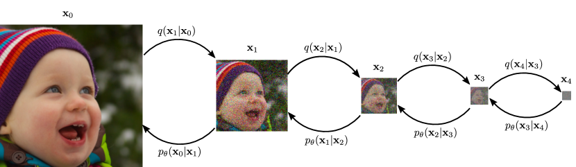
Figure 1: Upsampling Diffusion Probabilistic Model scheme for 5 diffusion steps ($L=4$).

2 Related Work

Diffusion models are latent variable models defined through a diffusion probabilistic model. Where on one side we have the data $\mathbf{x}_{0}\sim q_{\mathbf{x}_{0}}$ and on the far side we have pure noise $\mathbf{x}_{L}\sim q_{\mathbf{x}_{L}}$, both are related to each other using a Markovian diffusion process, where the forward process is defined by the joint distribution $q(\mathbf{x}_{0:L})$ and the learned reverse process by $p_{\theta}(\mathbf{x}_{0:L})$.

Using the Markov chain property we have

$$p_{\theta}(\mathbf{x}_{0:L})=p(\mathbf{x}_{L})\prod_{l=1}^{L}p_{\theta}(\mathbf{x}_{l-1}|\mathbf{x}_{l}),$$ (1)

and

$$q(\mathbf{x}_{1:L}|\mathbf{x}_{0})=\prod_{l=1}^{L}q(\mathbf{x}_{l}|\mathbf{x}_{l-1}),$$ (2)

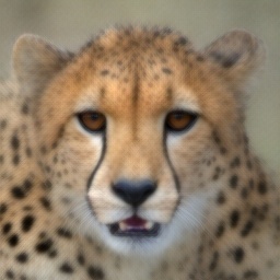
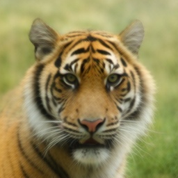
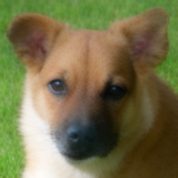
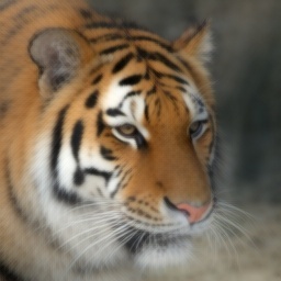
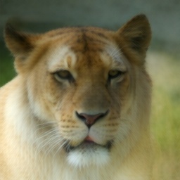
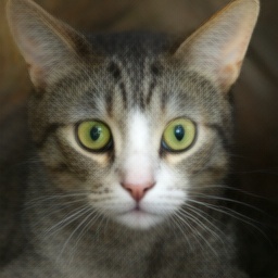
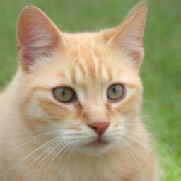
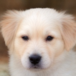
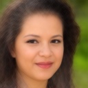
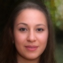
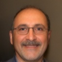
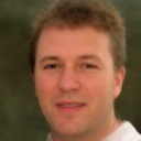
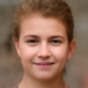
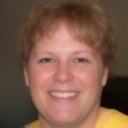
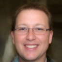
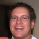
Figure 2: Generated $256\times 256$ images of AFHQ [7] (Top two rows) and $128\times 128$ images of FFHQ [20] (bottom two rows) using unconditional UDPM. UDPM requires only $6$ and $7$ diffusion steps for generating images from FFHQ and AFHQv2 respectively.

As stated in previous literature [14, 9, 33], the common approach is to assume that the Markov chain is constructed by normal distributions defined by

$$p_{\theta}(\mathbf{x}_{l-1}|\mathbf{x}_{l}):=\mathcal{N}(\mu^{(l)}_{\theta}(\mathbf{x}_{l}),\Sigma^{(l)}_{\theta}(\mathbf{x}_{l})),$$ (3)

and

$$q(\mathbf{x}_{l}|\mathbf{x}_{l-1}):=\mathcal{N}(\sqrt{1-\beta_{l}}\mathbf{x}_{l-1},\beta_{l}\mathbf{I}),$$ (4)

where $\beta_{1},\beta_{2},\ldots\beta_{L}$ are hyper-parameters that control the diffusion process noise levels.

By learning the reverse process $p_{\theta}(\mathbf{x}_{l-1}|\mathbf{x}_{l})$ using a deep neural network, one may generate samples from the data distribution by running the reverse process. Starting from pure noise $\mathbf{x}\sim\mathcal{N}(0,\mathbf{I})$ then progressively predicting the next step of the reverse process until reaching $\mathbf{x}_{0}$.

This principle has shown over the past couple of years marvelous performance in generating realistic-looking images [9, 28, 14, 33, 25, 21, 12, 32, 1]. However, as noted by [14], the number of diffusion steps $L$ is required to be large in order for the model to produce please looking images.

In recent years, many works utilized diffusion models for image manipulation and reconstruction tasks [36, 30], where a denoising network is trained to learn the prior distribution of the data. At test time, some conditioning mechanism is combined with the learned prior to solving very challenging imaging tasks [3, 2, 8]. Note that our novel adaptive diffusion ingredient can be incorporated into any conditional sampling scheme that is based on diffusion models.

The works in [36, 30] addressed the problems of deblurring and super-resolution using diffusion models. These works try to deblur [36] or increase the resolution [30] of an input blurry or low-res image. They do so by adding blur or downsampling to each noise step. Yet, unlike our work, their goal is not image generation but rather image reconstruction from a given degraded image. Therefore, their trained model is significantly different from ours despite the fact that they bear similarity to our work in the sense that they do not only denoise the image in each step but perform a reconstruction step.

Cold diffusion [4] performs diffusion steps by replacing the steps of noise addition with steps of blending with another image or other general steps. Also, that work is very different from our work as the goal here is to show that it is possible to replace denoising with other operations and not to show that it is possible to make the process more efficient computationally. In the supplementary material, we present an ablation study where we reduce the added noise during the forward process.

A concurrent effort [13, 18] suggests replacing the denoising steps by learning the wavelet coefficients of the high frequencies and they show it can reduce the number of diffusion steps. Our work differs from theirs by the fact that we rely on an upsampling with additive noise step, we show more datasets in our experiments and we also exhibit an interpretable latent space, which is a lacking component in many of the recent diffusion models.

Many works tried to accelerate the sampling procedure of denoising diffusion model [35, 19, 23, 24, 10], they focus only on reducing the number of sampling steps, while ignoring the diffusion structure itself. By contrast, in this work, we propose to not only degrade the signal over the noise domain but also in the spatial domain and therefore “dissolve” the signal much faster.

3 Method

Traditional denoising diffusion models assume that the probabilistic Markov process is defined by (3) and (4). These equations construct forward and backward processes that progress by adding and removing noise respectively. In this work, we generalize this scheme by adding an additional degradation element to the forward process, in which we subsample the variable spatial dimension when proceeding in the forward process, and upsample it when reversing the process.

3.1 Upsampling Diffusion Probabilistic Model

We begin by redefining the marginal distributions of the forward and reverse processes

$$q(\mathbf{x}_{l}|\mathbf{x}_{l-1}):=\mathcal{N}(\sqrt{1-\beta_{l}}\mathcal{H}\mathbf{x}_{l-1},\beta_{l}\mathbf{I}),$$ (5)

and

$$p_{\theta}(\mathbf{x}_{l-1}|\mathbf{x}_{l}):=\mathcal{N}(\mu_{\theta}(\mathbf{x}_{l},l),\Sigma_{l}),$$ (6)

where in contrast to previous diffusion models that used $\mathcal{H}=I$, in this work we define the operator $\mathcal{H}$ as a downsampling operator, defined by applying a blur filter $\mathcal{W}$ followed by subsampling with stride $\gamma$. As a result, the forward diffusion process decreases the variables dimensions in addition to the increased noise levels.

In diffusion models, the goal is to maximize the expected value of the marginal distribution $p_{\theta}(\mathbf{x}_{0})$, which is applicable when bounded via the Evidence Lower Bound (ELBO). Formally,

$$\mathbb{E}[-\log p_{\theta}(\mathbf{x}_{0})] \leq\mathbb{E}_{q}\left[-\log\frac{p_{\theta}(\mathbf{x}_{0:L})}{q(\mathbf{x}_{1:L}|\mathbf{x}_{0})}\right]$$

$$=\mathbb{E}_{q}[D_{\text{KL}}(p(\mathbf{x}_{L})||q(\mathbf{x}_{L}|\mathbf{x}_{0}))$$

$$+\sum_{l=2}^{L}D_{\text{KL}}(p_{\theta}(\mathbf{x}_{l-1}|\mathbf{x}_{l})||q(\mathbf{x}_{l-1}|\mathbf{x}_{l},\mathbf{x}_{0})$$

$$-\log p_{\theta}(\mathbf{x}_{1}|\mathbf{x}_{0})],$$ (7)

where the last equality is shown in Appendix A.1. The right hand side of (7) can be minimized stochastically w.r.t. $\theta$ using gradient descent, where at each step a random $t$ is chosen and therefore a single term of (7) is optimized.

In order to be able to use (7) for training $p_{\theta}(\cdot)$, one needs to explicitly find $q(\mathbf{x}_{l-1}|\mathbf{x}_{l},\mathbf{x}_{0})$, for which we need to obtain $q(\mathbf{x}_{l}|\mathbf{x}_{0})$ first, and then using the Bayes theorem, we can derive $q(\mathbf{x}_{l-1}|\mathbf{x}_{l},\mathbf{x}_{0})$. To do so, we first present the following lemma 1 (see Appendix A.2)

Lemma 1.

Let $\mathbf{e}\stackrel{{\scriptstyle iid}}{{\sim}}\mathcal{N}(0,\mathbf{I})\in\mathbb{R}^{N}$ and $\mathcal{H}=\mathcal{S}_{\gamma}\mathcal{W}$, where $\mathcal{S}_{\gamma}$ is a subsampling operator with stride $\gamma$ and $\mathcal{W}$ is a blur operator with blur kernel $\mathbf{w}$. Then if the support of $\mathbf{w}$ is at most $\gamma$ we have $\mathcal{H}\mathbf{e}\stackrel{{\scriptstyle iid}}{{\sim}}\mathcal{N}(0,\|\mathbf{w}\|_{2}^{2}\mathbf{I})$.

If Lemma 1 holds, then by assuming that $\|\mathbf{w}\|_{2}^{2}=1$, we get the following result (see Appendix A.3)

$$q(\mathbf{x}_{l}|\mathbf{x}_{0})=\mathcal{N}(\sqrt{\bar{\alpha}_{l}}\mathcal{H}^{l}\mathbf{x}_{0},(1-\bar{\alpha}_{l})\mathbf{I}),$$ (8)

where $\alpha_{l}=1-\beta_{l}$, and $\bar{\alpha}_{l}=\prod_{k=0}^{l}\alpha_{k}$. Using (8), we can obtain $\mathbf{x}_{t}$ from $\mathbf{x}_{0}$ simply by applying $\mathcal{H}$ $l$-times on $\mathbf{x}_{0}$, then using the traditional denoising diffusion noising scheme.

Given $q(\mathbf{x}_{l}|\mathbf{x}_{0})$, we can use the Bayes theorem and utilize the Markov chain property to get

$$q(\mathbf{x}_{l-1}|\mathbf{x}_{l},\mathbf{x}_{0})=\frac{q(\mathbf{x}_{l}|\mathbf{x}_{l-1})q(\mathbf{x}_{l-1}|\mathbf{x}_{0})}{q(\mathbf{x}_{l}|\mathbf{x}_{0})},$$

which as we show in Appendix A.4, is of the following form

$$q(\mathbf{x}_{l-1}|\mathbf{x}_{l},\mathbf{x}_{0})=\mathcal{N}(\mu(\mathbf{x}_{l},\mathbf{x}_{0},l),\Sigma_{l}),$$ (9)

where

$$\Sigma_{l}=\left(\frac{\alpha_{l}}{\beta_{l}}\mathcal{H}^{T}\mathcal{H}+\frac{1}{1-\bar{\alpha}_{l-1}}\mathbf{I}\right)^{-1},$$ (10)

and

$$\mu(\mathbf{x}_{l},\mathbf{x}_{0},l)=\Sigma_{l}\left(\frac{\sqrt{\alpha_{l}}}{\beta_{l}}\mathcal{H}^{T}\mathbf{x}_{l}+\frac{\sqrt{\bar{\alpha}_{l-1}}}{1-\bar{\alpha}_{l-1}}\mathcal{H}^{l-1}\mathbf{x}_{0}\right).$$ (11)

Although expression (10) seems to be implacable, in practice it can be implemented efficiently using the Discrete Fourier Transform and the poly-phase filtering identity used in [16, 5], where $\mathcal{H}^{T}\mathcal{H}$ is equivalent to convolution between $\mathbf{w}$ and its flipped version, followed by subsampling with stride $\gamma$ (see Appendix A.5 for more details.)

As can be obtained by (9), the true posterior $q(\mathbf{x}_{l-1}|\mathbf{x}_{l},\mathbf{x}_{0})$ in this setup is normal with parameters $(\mu(\mathbf{x}_{l},\mathbf{x}_{0},l),\Sigma_{l})$. Therefore, we assume that $p_{\theta}(\cdot)$ is also a normal distribution with parameters $(\mu_{\theta},\Sigma_{l})$, where $\mu_{\theta}$ is parameterized by a deep neural network with learned parameters $\theta$. We use this for minimizing (7) stochastically.

For normal distributions, a single term of the bound (7) is equivalent to

$$\ell^{(l)} =D_{\text{KL}}(p_{\theta}(\mathbf{x}_{l-1}|\mathbf{x}_{l})||q(\mathbf{x}_{l-1}|\mathbf{x}_{l},\mathbf{x}_{0})$$

$$=C_{l}+\frac{1}{2}(\mu_{\theta}-\mu_{l})^{T}\Sigma_{l}^{-1}(\mu_{\theta}-\mu_{l}),$$ (12)

where $C_{l}$ is a constant values not depending on $\theta$.

From our experiments and following [9, 14], training $p_{\theta}$ to predict $\mu$ directly leads to worse results. Therefore, we train the network to predict the second term in (11), i.e. to estimate $\mathcal{H}^{l-1}\mathbf{x}_{0}$ from $\mathbf{x}_{l}$. As a result, minimizing (12) can be simplified to minimizing the following term

$$\tilde{\ell}^{(l)}_{\text{simple}}=(f_{\theta}(\mathbf{x}_{l})-\mathcal{H}^{t-1}\mathbf{x}_{0})^{T}\Sigma(\mathbf{f}_{\theta}(\mathbf{x}_{l})-\mathcal{H}^{t-1}\mathbf{x}_{0}),$$ (13)

where $f_{\theta}(\cdot)$ is a deep neural network. By the definition of $\Sigma_{l}$, it is easy to show that it is a diagonal positive matrix, therefore it can be dropped. Furthermore, we found it better to predict $\mathbf{x}_{0}$ instead of its downsampled version $\mathcal{H}^{l-1}\mathbf{x}_{0}$. As a result, one may simplify the objective to the following term

$$\ell^{(l)}_{\text{simple}}=\|f_{\theta}(\mathbf{x}_{l})-\mathbf{x}_{0}\|_{2}^{2},$$ (14)

An overview of the training scheme is presented in Algorithm 1 and Figure 3.

Algorithm 1 UDPM training algorithm

0:  $f_{\theta}(\cdot),L,q(\mathbf{x})$

1:  while Not converged do

2:     $\mathbf{x}_{0}\sim q(\mathbf{x})$

3:     $l\in{1,2,\ldots,L}$

4:     $\mathbf{e}\sim N(0,I)$

5:     $\mathbf{x}_{l}=\sqrt{\bar{\alpha}_{l}}\mathcal{H}^{l}\mathbf{x}_{0}+\sqrt{1-\bar{\alpha_{l}}}\mathbf{e}$

6:     $\ell_{\text{simple}}=\|f_{\theta}(\mathbf{x}_{l})-\mathbf{x}_{0}\|_{2}^{2}$

7:     Adam step on $\ell_{\text{simple}}$

8:  end while

9:  return $\mathbf{x}_{0}$

3.2 Image Generation using UDPM

The Upsampling Diffusion Probabilistic Model (UDPM) presented in the previous section proposes a new ingredient for capturing the true implicit data distribution $q_{\mathbf{x}_{0}}$ of a given dataset. The remaining question is how it can be utilized for sampling from $q_{\mathbf{x}_{0}}$.

Given a deep neural network $f_{\theta}$ trained to predict $\mathbf{x}_{0}$ from $\mathbf{x}_{l}$, we begin with a pure normal noise sample $\mathbf{x}_{L}\sim\mathcal{N}(0,I)$. Subsequently, by substituting $\hat{\mathbf{x}}_{0}:=f_{\theta}(\mathbf{x}_{l})$ into equation (11), we can estimate $\mu_{L}$. Then the next reverse diffusion step $\mathbf{x}_{L-1}$ can be obtained by sampling from $\mathcal{N}(\mu_{L},\Sigma_{L})$. By iteratively repeating these steps $L$ times, we can acquire a sample $\mathbf{x}_{0}\sim p_{\theta}(\mathbf{x}_{0})$, as outlined in Algorithm 2.

Sampling the posterior requires parameterizing $\mathcal{N}(\mu_{l},\Sigma_{l})$ in the form of

$$\mathbf{x}_{l-1}=\mu_{l}+\Sigma_{l}^{\frac{1}{2}}\mathbf{e}$$

where $\mathbf{e}\sim\mathcal{N}(0,I)$ with the same dimensions as $\mathbf{x}_{l-1}$. This requires having access to $\Sigma^{\frac{1}{2}}_{l}$, which due to the structure of $\Sigma_{l}$, it is possible to apply it on $\mathbf{e}$ efficiently, as shown in A.6. The sampling procedure is summarized in Algorithm 2. The overview of both the training and sampling procedure is provided in Figure 3.

Algorithm 2 UDPM sampling algorithm

0:  $f_{\theta}(\cdot),L$

1:  $\mathbf{x}_{L}\sim\mathcal{N}(0,I)$

2:  for all $l=L,\ldots,1$ do

3:     $\Sigma=\left(\frac{\alpha_{l}}{\beta_{l}}\mathcal{H}^{T}\mathcal{H}+\frac{1}{1-\bar{\alpha}_{l}}\mathbf{I}\right)^{-1}$

4:     $\mu_{\theta}=\Sigma\left[\frac{\sqrt{\alpha_{l}}}{\beta_{l}}\mathcal{H}^{T}\mathbf{x}_{l}+\frac{\sqrt{\bar{\alpha}_{l-1}}}{1-\bar{\alpha}_{l-1}}\mathcal{H}^{l-1}f^{(l)}_{\theta}(\mathbf{x}_{l})\right]$

5:     $\mathbf{x}_{l-1}\sim\mathcal{N}(\mu_{\theta},\Sigma)$

6:  end for

7:  return $\mathbf{x}_{0}$

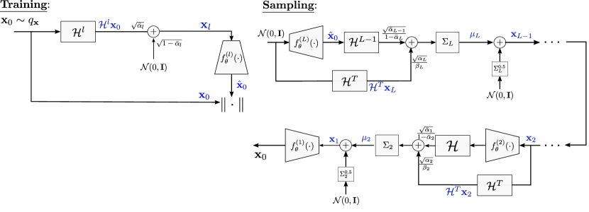
Figure 3: The training and sampling procedures of UDPM. During the training phase, an image $\mathbf{x}_{0}$ is randomly selected from the dataset $q_{\mathbf{x}_{0}}$. It is then corrupted using (8) to obtain a downsampled noisy version $\mathbf{x}_{l}$. Which is then plugged into a deep neural network $f_{\theta}^{(l)}(\cdot)$ for training it to predict $\mathbf{x}_{0}$. In the sampling phase, a pure white Gaussian noise $\mathbf{x}_{L}\sim\mathcal{N}(0,\mathbf{I})$ is generated. This noise is passed through the network $f_{\theta}^{(L)}(\cdot)$ to estimate $\mathbf{x}_{0}$. The estimated $\mathbf{x}_{0}$ is then downsampled $L-1$ times, and equation (11) is used to compute $\mu_{L}$, with $\Sigma_{L}$ obtained from equation (10). Afterwards, $\mathbf{x}_{L-1}$ is drawn from $\mathcal{N}(\mu_{L},\Sigma_{L})$ using the technique described in Appendix A.6. By repeating this procedure for $L$ iterations, the final sample $\mathbf{x}_{0}$ is obtained.

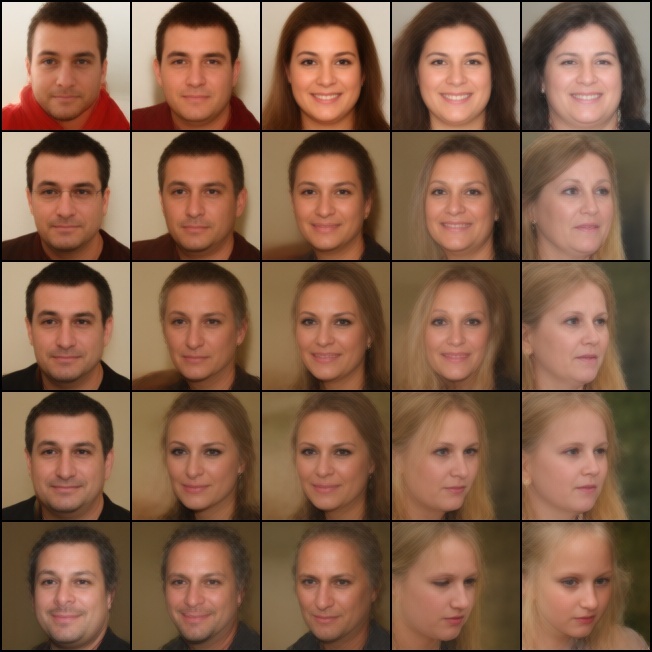
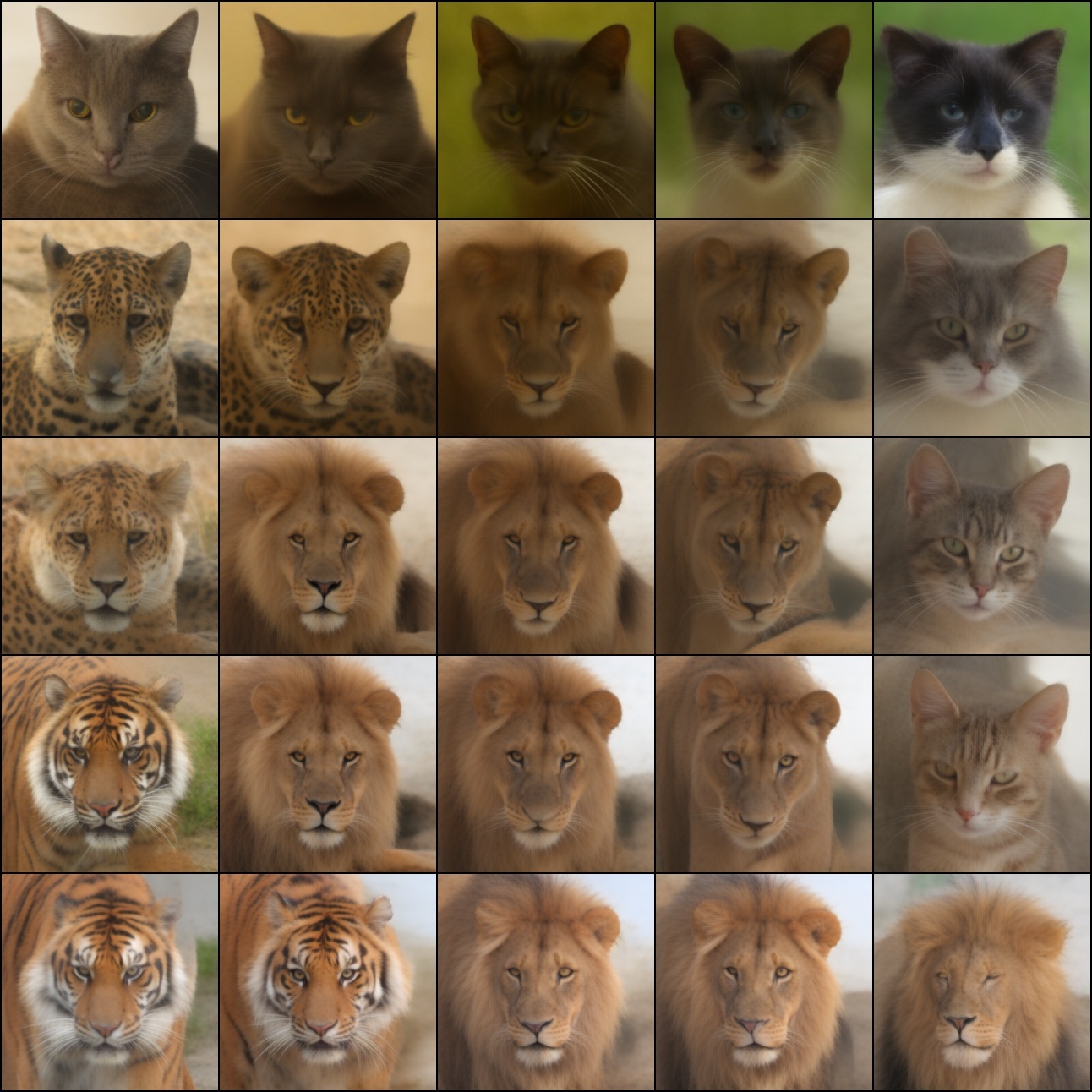
Figure 4: Latent space interpolation example. The four corner images are interpolated by a weighted mixture of their latent noises, such that the other images are “in-between” images from the latent perspective, similar to what has been done in GANs [20].

4 Experiments

In this section, we present the evaluation of our method UDPM under multiple scenarios. We tested our method on FFHQ [20], AFHQv2 [7], LSUN horses [37], and imagenet [29] datasets. Here we focus on the qualitative performance of UDPM and demonstrate its interpolatable latent space. In the sup. mat. we provide more results.

In all of our tests, we set the number of diffusion steps $L$ such that the dimensions of $\mathbf{x}_{L}$ are $2\times 2$, that is $L=\log_{\gamma}(\min\{H,W\})-1$, where $H$ and $W$ denote the dataset images height and width respectively.

We set $\gamma=2$ and use a uniform box filter of size $2\times 2$ as the downsampling kernel $\mathbf{w}$. We then normalize using its norm $\|\mathbf{w}\|$ and use it to construct the downsampling operator $\mathcal{H}$.

We follow the continuous-time scheme shown by [6], where instead of constraining the training of $f_{\theta}(\cdot)$ on $L$ noise levels we train using infinite noise levels, i.e. we generalize $l$ to be a continuous variable in the interval $[0,1]$, where $l=0$ is the real data domain and $l=1$ is the pure noise domain. We found this step to be very significant, as it improved the results dramatically. Under this setup, we define the down-sampling factor of $\mathcal{H}$ by $s(l)=\gamma^{\lceil L*l\rceil}$, in other words, we divide the interval $[0,1]$ into $L$ intervals and relate each interval to a single scaling factor.

Similar to [6] we set the noise scheduler by choosing $\bar{\alpha}_{l}$ and then derive the other noise parameters $\alpha_{l}$ and $\beta_{l}$ from it. Specifically, we chose

$$\bar{\alpha_{l}}=\frac{1-\sin(0.5\pi l)}{(\sum_{i}w_{i})^{2s(l)}}$$ (15)

where the denominator normalizes the SNR (Signal-to-Noise Ratio) such that it becomes invariant to the scaling of $\sum_{i}w_{i}$ obtained when applying $\mathcal{H}$.

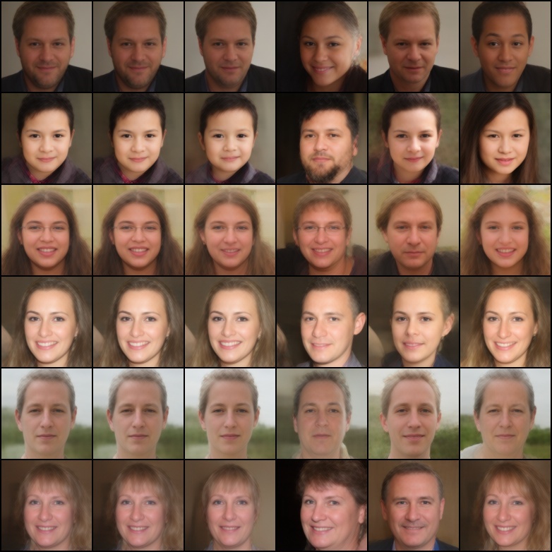
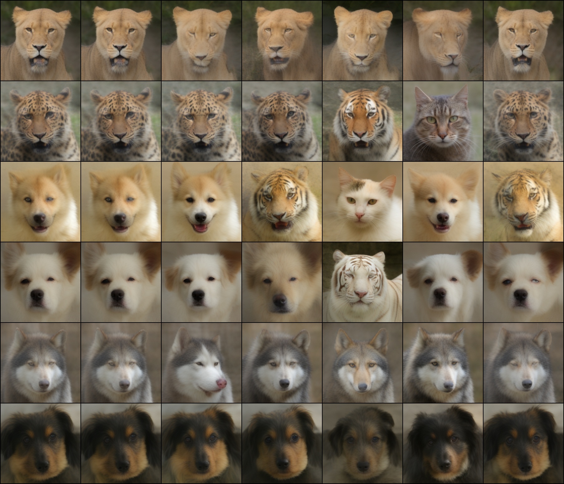
Figure 5: Latent space perturbation. The original images are on the left, then the images generated by adding a small noise to the latent noise from diffusion step $l$, starting from diffusion step $l=L$ (second images from the left) to the first diffusion step $l=1$ (the images on the right). Along each column, the same noise was used in order to give a better understanding of the representation

4.1 Unconditional Generation

In the unconditional scheme we evaluate our method UDPM on three different datasets, FFHQ, AFHQv2 and LSUN horses datasets, where each dataset contains $50K$, $14K$, and $2M$ images respectively. For FFHQ we train UDPM to generate $256\times 256$ and $128\times 128$ face images with $L=7$ and $L=6$ respectively. Similarly, for AFHQv2 we train UDPM to generate $256\times 256$ animal images with $L=7$. While for LSUN horses dataset UDPM is trained to generate $64\times 64$ images with $L=5$.

We use a variant of the UNet architecture used in [28], where we use six scales with self-attention in the lower three scales. Specifically, we set “block_out_channels” to $(128,128,256,256,512,512)$ and “attention_head_dim” to $64$, and leave all the remaining hyper-parameters to their default values. For enabling the network to receive an arbitrary input size, we add a bilinear upsampling layer that resamples the input to the desired shape. As a result, the total number of learned parameters in the network is 120.25M. We train the network for $300K$ Adam [22] steps to minimize (14) in addition to the VGG perceptual term from [38] weighted by $0.1$. We set the batch size and learning rate to $256$ and $10^{-4}$ respectively, and follow previous literature by using weight exponential moving averaging (EMA) with parameter 0.9999. The generation results of UDPM on FFHQ and AFHQv2 can be seen in Figure 2 as well as many other examples in the supplementary material where we provide generation results of the LSUN horses dataset as well.

One major benefit of our method compared to the traditional denoising diffusion setup is the significant decrease in the number of iterations, which as a result enables us to interpolate the latent space and therefore generate “intermediate” images of two generated images, similar to what can be done in Generative Adversarial Networks [20, 17]. As can be seen in Figure 4, where the images in the corners of each sub-figure are generated randomly, and by averaging their noise maps we can generate interpolating images (the middle ones). By controlling the averaging weight one may control how much the image should look like the image on the left or the right.

Another advantage of our method compared to standard denoising diffusion models is that we can better interpret the latent space by perturbing each diffusion step on its own and examining the results. Note that one may modify the noise map in one direction to modify the age of the person, expression, color, etc. Examples of that are presented in Figures 5. Note that the dominant diffusion steps that significantly control the pose, expression, or general look of the generated images are steps 4 and 3. By choosing a direction in the latent space one may be able to modify the characteristics of the generated output, for instance, make the person smile, change the pose, modify the gender, etc., which are features yet to be explored in diffusion models. Notice that these are just initial results and we believe that the latent space of UDPM should be further analyzed.

4.2 Classes conditional generation

We also propose a conditional generation scheme for UDPM, where we use the label encoding block from [11, 26] combined with the cross-attention mechanism from [28] in order to control the generation class. We evaluate our method UDPM on the popular ImageNet dataset [29], which consists of 1.3M images of 1000 different classes. In this case, we train UDPM to generate $64\times 64$ images with $L=5$.

Similar to the unconditional scenario, we use a variant of the UNet architecture used in [28], with the same hyper-parameters except for the attention layers, which we replace with cross-attention layers [28] for the conditioning mechanism, where we encode the class into a 1024 dimension vector used for cross-attention. Here we also use the same bilinear upsampling layer that resamples the input to the desired shape as in the unconditional case. Under these circumstances, the total number of learned parameters is 186.91M. We train the network for $700K$ Adam [22] steps to minimize (14) in addition to the VGG perceptual term. We set the batch size to $256$, the learning rate to $10^{-4}$, and use EMA similar to the unconditional training case.

When sampling we follow the classifier-free approach [15], where at training time we drop 0.1 of the classes and use traditional classifier-free sampling conditioning. The results for this case with multiple guidance scale values are presented in the supplementary material.

4.3 Limitation

Note that the results we get with our approach are softer than other diffusion models. Yet, we believe that this is due to our computational constraints. During training, we see that our model continues to improve and gets sharper results when we increase the batch size and number of iterations. Yet, due to a lack of resources, we are limited in the number of training iterations and the size of the data we can use. In the sup. mat. we show results on additional datasets such as ImageNet, but also there we are limited to a resolution of $64\times 64$. Yet, we believe that our method can be easily applied given the necessary computational resources to the full resolution and that our work provides a proof of concept for the UDPM strategy. Notice that once our method is trained, it is expected to accelerate image generation and editing due to two important reasons: (i) it uses much fewer iterations; and (ii) it has an interpolatable latent space, which is lacking in other diffusion models. Overall, our approach has the potential to enable much faster image generation and editing than what is currently possible and we hope that it will be used to train on large datasets such as LION-400, which contains 400 million images, or LION-5B [31], which contains 5.85 Billion images.

5 Conclusion

We have proposed a new diffusion-based generative model called the Upsampling Diffusion Probabilistic Model (UPDM). Our approach reduces the number of diffusion steps required to produce high-quality images, making it significantly more efficient than previous solutions.

We have demonstrated the effectiveness of our approach on four different datasets, FFHQ, AFHQ, LSUN horses, and ImageNet, showing that it is capable of producing high-quality images with only 7 diffusion steps for the largest images ($256\times 256$), and 5 diffusion steps for the smallest ($64\times 64$), which is two orders of magnitude better compared to the original diffusion models work and significantly better than current state-of-the-art works dedicated to diffusion sampling acceleration.

Furthermore, we have shown that our interpolatable latent space has potential for further exploration, particularly in the realm of image editing. Based on the initial results shown in the paper, it contains semantic directions, such as making people smile or changing their age. We believe that it can be used to perform editing operations like the ones performed in styleGAN while maintaining better generation capabilities and favorable properties of diffusion.

Acknowledgement. This work is partially supported by ERC-StG (No. 757497). S. Abu-Hussein is thankful to the Neubauer family foundation for their gracious support.

UDPM: Upsampling Diffusion Probabilistic Models – Supplementary Material

We provide here the extended derviation of our UDPM model in Section A, an ablation study on the noise scheduler in Section B and additional visual results that include ImageNet in Section C

Appendix A Extended Derivations

A.1 Evidence Lower Bound

From the traditional Evidence Lower Bound (ELBO) we have $\mathbb{E}[-\log p_{\theta}(\mathbf{x}_{0})]\leq\mathbb{E}_{q}\left[\log\frac{p_{\theta}(\mathbf{x}_{0:L})}{q(\mathbf{x}_{1:L}|\mathbf{x}_{0})}\right]$, therefore

$$\mathbb{E}[-\log p_{\theta}(\mathbf{x}_{0})] \leq\mathbb{E}_{q}\left[\log\frac{p_{\theta}(\mathbf{x}_{0:L})}{q(\mathbf{x}_{1:L}|\mathbf{x}_{0})}\right]=\mathbb{E}_{q}\left[-\log p(\mathbf{x}_{T})-\sum_{l=1}^{L}\log\frac{p_{\theta}(\mathbf{x}_{l-1}|\mathbf{x}_{l})}{q(\mathbf{x}_{l}|\mathbf{x}_{l-1})}\right]$$

$$=\mathbb{E}_{q}\left[-\log p(\mathbf{x}_{T})-\sum_{l=2}^{L}\log\frac{p_{\theta}(\mathbf{x}_{l-1}|\mathbf{x}_{l})}{q(\mathbf{x}_{l}|\mathbf{x}_{l-1})}-\log\frac{p_{\theta}(\mathbf{x}_{0}|\mathbf{x}_{1})}{q(\mathbf{x}_{1}|\mathbf{x}_{0})}\right]$$

$$\stackrel{{\scriptstyle(\star)}}{{=}}\mathbb{E}_{q}\left[-\log p(\mathbf{x}_{T})-\sum_{l=2}^{L}\log\frac{p_{\theta}(\mathbf{x}_{l-1}|\mathbf{x}_{l})q(x_{l-1}|\mathbf{x}_{l})}{q(\mathbf{x}_{l-1}|\mathbf{x}_{l},\mathbf{x}_{0})q(\mathbf{x}_{l}|\mathbf{x}_{0})}-\log\frac{p_{\theta}(\mathbf{x}_{0}|\mathbf{x}_{1})}{q(\mathbf{x}_{1}|\mathbf{x}_{0})}\right]$$

$$=\mathbb{E}_{q}\left[-\log p(\mathbf{x}_{T})-\sum_{l=2}^{L}\log\frac{p_{\theta}(\mathbf{x}_{l-1}|\mathbf{x}_{l})}{q(\mathbf{x}_{l-1}|\mathbf{x}_{l},\mathbf{x}_{0})}-\sum_{l=2}^{L}\log q(\mathbf{x}_{l-1}|\mathbf{x}_{l})+\sum_{l=2}^{L}q(\mathbf{x}_{l}|\mathbf{x}_{0})-\log\frac{p_{\theta}(\mathbf{x}_{0}|\mathbf{x}_{1})}{q(\mathbf{x}_{1}|\mathbf{x}_{0})}\right]$$

$$=\mathbb{E}_{q}\left[-\log p(\mathbf{x}_{T})-\sum_{l=2}^{L}\log\frac{p_{\theta}(\mathbf{x}_{l-1}|\mathbf{x}_{l})}{q(\mathbf{x}_{l-1}|\mathbf{x}_{l},\mathbf{x}_{0})}-\cancel{\log q(\mathbf{x}_{1}|\mathbf{x}_{0})}+\log q(\mathbf{x}_{L}|\mathbf{x}_{0})-\log\frac{p_{\theta}(\mathbf{x}_{0}|\mathbf{x}_{1})}{\cancel{q(\mathbf{x}_{1}|\mathbf{x}_{0})}}\right]$$

$$=\mathbb{E}_{q}\left[-\log\frac{p(\mathbf{x}_{T})}{q(\mathbf{x}_{L}|\mathbf{x}_{0})}-\sum_{l=2}^{L}\log\frac{p_{\theta}(\mathbf{x}_{l-1}|\mathbf{x}_{l})}{q(\mathbf{x}_{l-1}|\mathbf{x}_{l},\mathbf{x}_{0})}-\log p_{\theta}(\mathbf{x}_{0}|\mathbf{x}_{1})\right]$$

$$=\mathbb{E}_{q}\left[D_{\text{KL}}(p(\mathbf{x}_{T})||q(\mathbf{x}_{L}|\mathbf{x}_{0}))+\sum_{l=2}^{L}D_{\text{KL}}(p_{\theta}(\mathbf{x}_{l-1}|\mathbf{x}_{l})||q(\mathbf{x}_{l-1}|\mathbf{x}_{l},\mathbf{x}_{0}))-\log p_{\theta}(\mathbf{x}_{0}|\mathbf{x}_{1})\right]$$

where in $(\star)$ Bayes was used, particularly

$$q(\mathbf{x}_{l}|\mathbf{x}_{l-1},\mathbf{x}_{0})=\frac{q(\mathbf{x}_{l-1},\mathbf{x}_{l}|\mathbf{x}_{0})}{q(\mathbf{x}_{l-1}|\mathbf{x}_{0})}=\frac{q(\mathbf{x}_{l-1}|\mathbf{x}_{l},\mathbf{x}_{0})q(\mathbf{x}_{l}|\mathbf{x}_{0})}{q(\mathbf{x}_{l-1}|\mathbf{x}_{0})}$$

A.2 Lemma 1

Proof.

The characteristic function of a Normal vector $\mathbf{e}\sim\mathcal{N}(\mu,\Sigma)$ is in the form

$$\phi_{\mathbf{e}}(\mathbf{t})=\mathbb{E}[\exp(i\mathbf{t}^{T}\mathbf{e})]=\exp(i\mathbf{t}^{T}\mu-\frac{1}{2}\mathbf{t}^{T}\Sigma\mathbf{t})$$ (16)

when $\mu=0$ and $\Sigma=\mathbf{I}$ we get

$$\phi_{\mathbf{e}}(\mathbf{t})=\exp(-\frac{1}{2}\mathbf{t}^{T}\mathbf{t})$$

Therefore to prove the first claim of the lemma, it is sufficient to prove that $\mathcal{H}\mathbf{e}$ has a characteristic function of the form (16). Denote the transpose operator of $\mathcal{H}$ by $\mathcal{H}^{T}$, which is defined as zero padding operator followed by applying a flipped version the kernel of $\mathcal{H}$, denoted by $\mathbf{w}$, Then

$$\phi_{\mathcal{H}\mathbf{e}}(\mathbf{t}) =\mathbb{E}[\exp(i\mathbf{t}^{T}(\mathcal{H}\mathbf{e})]=\mathbb{E}[\exp(i(\mathcal{H}^{T}\mathbf{t})^{T}\mathbf{e}]=\exp(i(\mathcal{H}^{T}\mathbf{t})^{T}\mu-\frac{1}{2}(\mathcal{H}^{T}\mathbf{t})^{T}\Sigma(\mathcal{H}^{T}\mathbf{t}))$$

$$=\exp(i\mathbf{t}^{T}\mathcal{H}\mu-\frac{1}{2}\mathbf{t}^{T}\mathcal{H}\Sigma\mathcal{H}^{T})\mathbf{t})\stackrel{{\scriptstyle\{\mu=0,\Sigma=I\}}}{{=}}\exp(-\frac{1}{2}\mathbf{t}^{T}\mathcal{H}\mathcal{H}^{T})\mathbf{t})$$

$$\Rightarrow\mathcal{H}\mathbf{e}\sim\mathcal{N}(0,\mathcal{H}\mathcal{H}^{T})$$

All that remains is to express $\mathcal{H}\mathcal{H}^{T}$ under the assumption on the downsampling kernel support. The operator $\mathcal{H}$ is defined as applying blur kernel $\mathbf{w}=[w_{-\lfloor\alpha/2\rfloor+1},\ldots,w_{0},\ldots w_{\lfloor\alpha/2\rfloor}]$ followed by subsampling with stride $\alpha$, which can be represented in matrix form by $\mathcal{H}=\mathcal{S}_{\alpha}\mathcal{W}$, where $\mathcal{S}_{\alpha}\in\mathbb{R}^{M\times N}$ and $\mathcal{W}\in\mathbb{R}^{N\times N}$. Specifically

$$\mathcal{S}_{\alpha}=\begin{pmatrix}1\ 0\ \ldots\ 0\ 0\ \ldots\ 0&\ldots&0\\ \underbrace{0\ \ldots\ 0}_{\alpha}\ 1\ 0\ \ldots\ 0&\ldots&0\\ \underbrace{0\ \ldots\ 0}_{\alpha}\ \underbrace{0\ \ldots\ 0}_{\alpha}\ 1&\ldots&0\\ \vdots&\vdots&\vdots\end{pmatrix}\\$$

$$\mathcal{W}_{\alpha}=\begin{pmatrix}w_{0}&w_{1}&\ldots&w_{\lfloor\alpha/2\rfloor}&0&\ldots&w_{-\lfloor\alpha/2\rfloor+1}&w_{-\lfloor\alpha/2\rfloor+2}&\ldots&w_{-1}\\ w_{-1}&w_{0}&\ldots&w_{\lfloor\alpha/2\rfloor}&0&\ldots&0&w_{-\lfloor\alpha/2\rfloor+1}&\ldots&w_{-2}\\ \vdots&&&\vdots&&&\vdots&&&\vdots\end{pmatrix}$$

Therefore we have

$$\mathcal{S}_{\alpha}\mathcal{W}=\begin{pmatrix}w_{0}&\ldots&w_{\lfloor\alpha/2\rfloor}&0&\ldots&0&\ldots&0&w_{-\lfloor\alpha/2\rfloor+1}&\ldots\\ 0&\ldots&0&w_{-\lfloor\alpha/2\rfloor+1}&\ldots&w_{\lfloor\alpha/2\rfloor}&\ldots&0&0&\ldots\\ \vdots&&&\vdots&&&\vdots&&&\vdots\end{pmatrix}$$ (17)

as can be observed from (17), the rows of $\mathcal{S_{\alpha}\mathcal{W}}$ do not intersect with each other, as a result we get

$$\mathcal{H}\mathcal{H}^{T}=\mathcal{S}_{\alpha}\mathcal{W}(\mathcal{S}_{\alpha}\mathcal{W})^{T}=\begin{pmatrix}\|\mathbf{w}\|_{2}^{2}&0&0&\ldots&0\\ 0&\|\mathbf{w}\|_{2}^{2}&0&\ldots&0\\ \vdots&\vdots&\vdots&\ldots&\vdots\\ 0&0&0&\ldots&\|\mathbf{w}\|_{2}^{2}\end{pmatrix}=\|\mathbf{w}\|_{2}^{2}\mathbf{I}$$ (18)

∎

A.3 Efficient representation of the forward process

Similar to earlier works, for efficient training, one would like to sample $\mathbf{x}_{l}$ directly using $\mathbf{x}_{0}$. Which is viable when assuming that the support of $\mathbf{w}$ is at most $\alpha$ and $\|w\|_{2}^{2}=1$

$$\mathbf{x}_{l} \stackrel{{\scriptstyle\eqref{eq:q_theta_def}}}{{=}}\sqrt{1-\beta_{l}}\mathcal{H}\mathbf{x}_{l-1}+\sqrt{\beta_{l}}\mathbf{e}_{1}=\sqrt{1-\beta_{l}}\mathcal{H}(\sqrt{1-\beta_{l-1}}\mathcal{H}\mathbf{x}_{l-2}+\sqrt{\beta_{l-1}}\mathbf{e}_{2})+\sqrt{\beta_{l}}\mathbf{e}_{1}$$

$$=\sqrt{1-\beta_{l}}\sqrt{1-\beta_{l-1}}\mathcal{H}^{2}\mathbf{x}_{l-2}+\sqrt{1-\beta_{l}}\sqrt{\beta_{l-1}}\mathcal{H}\mathbf{e}_{2}+\sqrt{\beta_{l}}\mathbf{e}_{1}$$

$$\stackrel{{\scriptstyle\eqref{lemma:sampled_gauss}}}{{=}}\sqrt{1-\beta_{l}}\sqrt{1-\beta_{l-1}}\mathcal{H}^{2}\mathbf{x}_{l-2}+\sqrt{1-\beta_{l}}\sqrt{\beta_{l-1}}\tilde{\mathbf{e}}_{2}+\sqrt{\beta_{l}}\mathbf{e}_{1}$$

$$=\sqrt{\gamma_{l}}\sqrt{\gamma_{l-1}}\mathcal{H}^{2}\mathbf{x}_{l-2}+\sqrt{\gamma_{l}}\sqrt{\beta_{l-1}}\tilde{\mathbf{e}}_{2}+\sqrt{\beta_{l}}\mathbf{e}_{1}$$

where $\gamma_{l}=1-\beta_{l}$, $\mathbf{e}_{1}\sim\mathcal{N}(0,\mathbf{I})$, and $\mathbf{e}_{2}\sim\mathcal{N}(0,\mathbf{I})$. By definition, $\mathbf{e}_{1}$ and $\mathbf{e}_{2}$ are independent identically distributed vectors, therefore

$$\mathbf{x}_{l} =\sqrt{\gamma_{l}}\sqrt{\gamma_{l-1}}\mathcal{H}^{2}\mathbf{x}_{l-2}+(\sqrt{\gamma_{l}}\sqrt{\beta_{l-1}}+\sqrt{\beta_{l}})\mathbf{e}$$

repeating the opening $l-2$ times similar to [14] gives

$$\mathbf{x}_{l}=\sqrt{\bar{\gamma}_{l}}\mathcal{H}^{l}\mathbf{x}_{0}+\sqrt{1-\bar{\gamma}_{l}}\mathbf{e}$$

where $\bar{\gamma}_{l}=\prod_{k=1}^{L}\gamma_{k}$ and $\mathbf{e}\sim\mathcal{N}(0,\mathbf{I})$.

A.4 Derivation of the posterior

Using Bayes theorem, we have for $l>1$

$$q(\mathbf{x}_{l-1}|\mathbf{x}_{l},\mathbf{x}_{0}) =\frac{q(\mathbf{x}_{l-1},\mathbf{x}_{l}|\mathbf{x}_{0})}{q(\mathbf{x}_{l}|\mathbf{x}_{0})}=\frac{q(\mathbf{x}_{l}|\mathbf{x}_{l-1},\cancel{\mathbf{x}}_{0})q(\mathbf{x}_{l-1}|\mathbf{x}_{0})}{q(\mathbf{x}_{l}|\mathbf{x}_{0})}\stackrel{{\scriptstyle\text{Markov}}}{{=}}\frac{q(\mathbf{x}_{l}|\mathbf{x}_{l-1})q(\mathbf{x}_{l-1}|\mathbf{x}_{0})}{q(\mathbf{x}_{l}|\mathbf{x}_{0})}$$

$$\stackrel{{\scriptstyle(\star\star)}}{{\propto}}\exp\left(-\frac{1}{2\beta_{l}}\|\mathbf{x}_{l}-\sqrt{\gamma_{l}}\mathcal{H}\mathbf{x}_{l-1}\|_{2}^{2}-\frac{1}{2(1-\bar{\gamma}_{l-1})}\|\mathbf{x}_{l-1}-\sqrt{\bar{\gamma}}_{l-1}\mathcal{H}^{l-1}\mathbf{x}_{0}\|_{2}^{2}\right)$$

$$=\exp(-\frac{1}{2\beta_{l}}(\mathbf{x}_{l}^{T}\mathbf{x}_{l}-2\sqrt{\gamma_{l}}\mathbf{x}_{l-1}^{T}\mathcal{H}^{T}\mathbf{x}_{l}+\gamma_{l}\mathbf{x}_{l-1}^{T}\mathcal{H}^{T}\mathcal{H}\mathbf{x}_{t-1})$$

$$-\frac{1}{2(1-\bar{\gamma}_{l-1})}(\mathbf{x}_{t-1}^{T}\mathbf{x}_{l-1}-2\sqrt{\bar{\gamma}_{l-1}}\mathbf{x}_{l-1}^{T}\mathcal{H}^{l-1}\mathbf{x}_{0}+\bar{\gamma}_{l-1}\mathbf{x}_{0}^{T}(\mathcal{H}^{l-1})^{T}\mathcal{H}^{l-1}\mathbf{x}_{0}))$$

$$\stackrel{{\scriptstyle(\star\star)}}{{\propto}}\exp\left\{-\frac{1}{2}\left[\mathbf{x}_{l-1}^{T}\left(\frac{\gamma_{t}}{\beta_{t}}\mathcal{H}^{T}\mathcal{H}+\frac{1}{1-\bar{\gamma}_{l-1}}\mathbf{I}\right)\mathbf{x}_{l-1}-2\mathbf{x}_{l-1}^{T}\left(\frac{\sqrt{\gamma}_{l}}{\beta_{l}}\mathcal{H}^{T}\mathbf{x}_{l}+\frac{\sqrt{\bar{\gamma}_{l-1}}}{1-\bar{\gamma}_{l}}\mathcal{H}^{l-1}\mathbf{x}_{0}\right)\right]\right\}$$

which is a Normal distribution form w.r.t. the random vector $\mathbf{x}_{l-1}$. Note that in $(\star\star)$ the proportional equivalence is with relation to $\mathbf{x}_{l-1}$. As a result, let $q(\mathbf{x}_{l-1}|\mathbf{x}_{l},\mathbf{x}_{0})=\mathcal{N}(\mu,\Sigma)$, then

$$\Sigma^{-1}=\frac{\gamma_{l}}{\beta_{l}}\mathcal{H}^{T}\mathcal{H}+\frac{1}{1-\bar{\gamma}_{l-1}}\mathbf{I}$$ (19)

and

$$\Sigma^{-1}\mu=\frac{\sqrt{\gamma_{l}}}{\beta_{l}}\mathcal{H}^{T}\mathbf{x}_{l}+\frac{\sqrt{\bar{\gamma}_{l-1}}}{1-\bar{\gamma}_{l-1}}\mathcal{H}^{l-1}\mathbf{x}_{0}$$ (20)

A.5 Mean and variance of the posterior

The terms in (19) and (20) seem hard to evaluate, however, in the following we present an efficient way to compute them. By definition $\mathcal{H}$ is structured from a circular convolution with a blur filter followed by a subsampling with stride $\alpha$. Therefore, one may use the poly-phase identity used in [16, 5], which states that $\mathcal{H}^{T}\mathcal{H}$ in this case is a circular convolution between the blur kernel $\mathbf{w}$ and its flipped version $\tilde{\mathbf{w}}$ followed by subsampling with factor $\alpha$, formally

$$\mathbf{h}=(\mathbf{w}\circledast flip(\mathbf{w}))\downarrow_{\alpha}$$

therefore, one may write $\mathcal{H}^{T}\mathcal{H}$ in the following form

$$\mathcal{H}^{T}\mathcal{H}=\mathcal{F}^{\star}\Lambda_{\mathbf{h}}\mathcal{F}$$ (21)

where $\mathcal{F}$ is the Discrete Fourier Transform (DFT), $\mathcal{F}^{\star}$ is the inverse DFT, and $\Lambda_{\mathbf{h}}$ is a diagonal operator representing the DFT transform of $\mathbf{h}$. By plugging (21) into (19) we get

$$\Sigma^{-1}=\frac{\gamma_{l}}{\beta_{l}}\mathcal{F}^{\star}\Lambda_{\mathbf{h}}\mathcal{F}+\frac{1}{1-\bar{\gamma}_{l-1}}\mathbf{I}=\frac{\gamma_{l}}{\beta_{l}}\mathcal{F}^{\star}\Lambda_{\mathbf{h}}\mathcal{F}+\frac{1}{1-\bar{\gamma}_{l-1}}\mathcal{F}^{\star}\mathcal{F}=\mathcal{F}^{\star}\left(\frac{\gamma_{l}}{\beta_{l}}\Lambda_{\mathbf{h}}+\frac{1}{1-\bar{\gamma}_{l-1}}\mathbf{I}\right)\mathcal{F}$$

equivalently

$$\Sigma=\mathcal{F}^{\star}\left(\frac{\gamma_{l}}{\beta_{l}}\Lambda_{\mathbf{h}}+\frac{1}{1-\bar{\gamma}_{l-1}}\mathbf{I}\right)^{-1}\mathcal{F}$$ (22)

Therefore, as can be observed from (22), applying $\Sigma$ is equivalent to applying the inverse of the filter $\left(\frac{\gamma_{l}}{\beta_{l}}\Lambda_{\mathbf{h}}+\frac{1}{1-\bar{\gamma}_{l-1}}\mathbf{I}\right)$, which can be performed efficiently using Fast Fourier Transform (FFT). As a result we have

$$\mu=\Sigma\left(\frac{\sqrt{\gamma_{l}}}{\beta_{l}}\mathcal{H}^{T}\mathbf{x}_{l}+\frac{\sqrt{\bar{\gamma}_{l-1}}}{1-\bar{\gamma}_{l-1}}\mathcal{H}^{l-1}\mathbf{x}_{0}\right)$$ (23)

A.6 Sampling the posterior

As discussed in section 3.2, the proposed generation scheme requires to sample from $\mathcal{N}(\mu_{l},\Sigma_{l})$ at each diffusion step, which due to the structure of $\Sigma_{l}$ is not naive, since $\Sigma_{l}^{0.5}$ is needed in order to use the parameterization $\mathbf{x}_{l-1}|\mathbf{x}_{l}=\mu_{l}(\mathbf{x}_{l})+\Sigma_{l}^{0.5}\mathbf{e}$ where $\mathbf{e}\sim\mathcal{N}(0,I)$. However, as we saw in section A.5, the operator $\Sigma_{l}$ is equivalent to applying a linear filter $\mathbf{h}$, therefore one may seek to find a filter $\mathbf{d}$ such that

$$\Sigma=\mathcal{F}^{\star}\Lambda_{\mathbf{h}}\mathcal{F}=\mathcal{F}^{\star}\Lambda_{\mathbf{d}}^{2}\mathcal{F}$$

equivalently, we can break the DFT of filter $\mathbf{h}$ to magnitude and phase such that

$$\text{DFT}\{\mathbf{h}\}=|\text{DFT}\{\mathbf{h}\}|e^{i\phi_{h}}=|\text{DFT}\{\mathbf{d}\}|^{2}e^{i2\phi_{h}}$$

therefore

$$|\text{DFT}\{\mathbf{d}\}|=\sqrt{|\text{DFT}\{\mathbf{h}\}|},\ \measuredangle|\text{DFT}\{\mathbf{d}\}|=\frac{1}{2}\arctan\frac{Im\{\text{DFT}\{\mathbf{h}\}\}}{Re\{\text{DFT}\{\mathbf{h}\}\}}$$ (24)

As a result, applying $\Sigma^{0.5}$ can be performed by employing the filter $\mathbf{d}$ defined in (24).

Appendix B Noise scheduler ablation

In addition to the noise scheduler in (15), we examined other choices used in previous literature [14, 9, 6]. For instance a cosine scheduler, where $\bar{\gamma}_{l}=\cos(0.5\pi l)$, or a linear scheduler with $\bar{\gamma}_{l}=1-l$. However, we saw that when training with less noise the results tend to look over-smoothed, as can be seen in Figure 6, where we compare our noise scheduler (15) to the cosine scheduler used in previous works. The usage of a less noisy scheduler can lead to smooth results, lacking fine details, particularly in heterogeneous regions such as in the background.

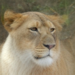
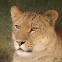
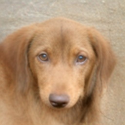
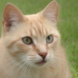
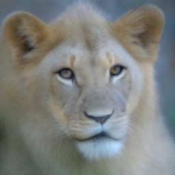
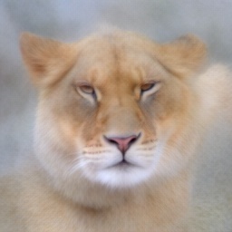
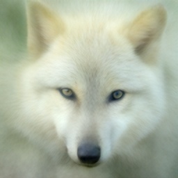
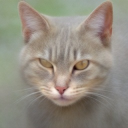
Figure 6: Top row: $256\times 256$ Images generated using UDPM trained on the AFHQv2 dataset [7] with the noise scheduler presented in (15). Bottom row: UDPM results trained on the same dataset with cosine noise scheduler $\bar{\gamma}_{l}=\cos(0.5\pi l)$. As can be seen, the results when using a weaker noise model tend to be smooth, especially in the background where the details are less homogeneous.

Appendix C Additional results

C.1 Latent space interpolation

As shown previously by [20], generative models have a very interesting property, where one may modify the latent variable of the generative model in order to control the “style” of the generated result, or for instance, given the latent variables of two images, one may interpolate the latent space and get an “in-between” images that in contrast to the pixel-domain interpolation, transition smoothly and naturally, as can be seen in Figures 7 and 8.

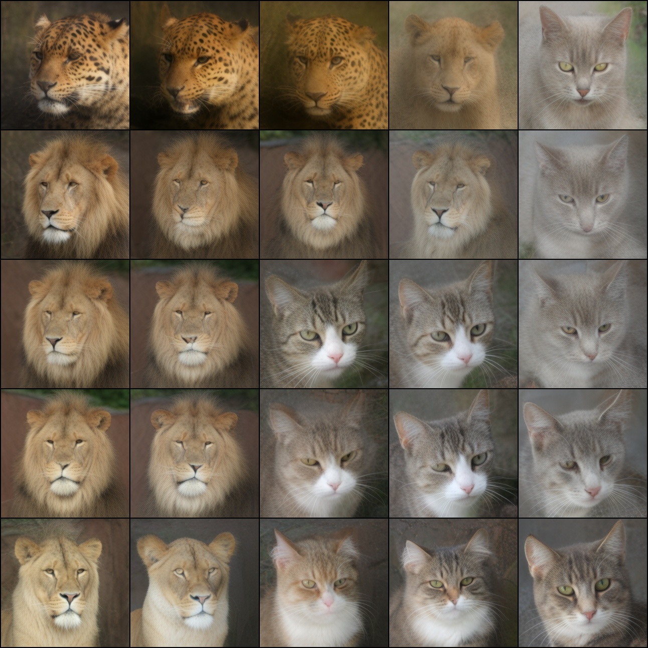
Figure 7: AFHQv2 [7] latent space interpolation example. The four corner images are interpolated by a weighted mixture of their latent noises, such that the other images are “in-between” images from the latent perspective, similar to what has been done in GANs [20]. All the images are of size $256\times 256$.

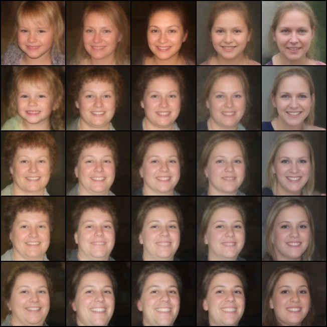
Figure 8: FFHQv2 [7] latent space interpolation example. The four corner images are interpolated by a weighted mixture of their latent noises, such that the other images are “in-between” images from the latent perspective, similar to what has been done in GANs [20]. All the images are of size $128\times 128$.

C.2 Latent space perturbation

Similar to what is presented in the main paper, we show additional latent variable perturbation in order to obtain better understanding of the latent space, where we add a small noise to a single diffusion step and see how it affects the generated result, as can be seen in Figures 9 and 10.

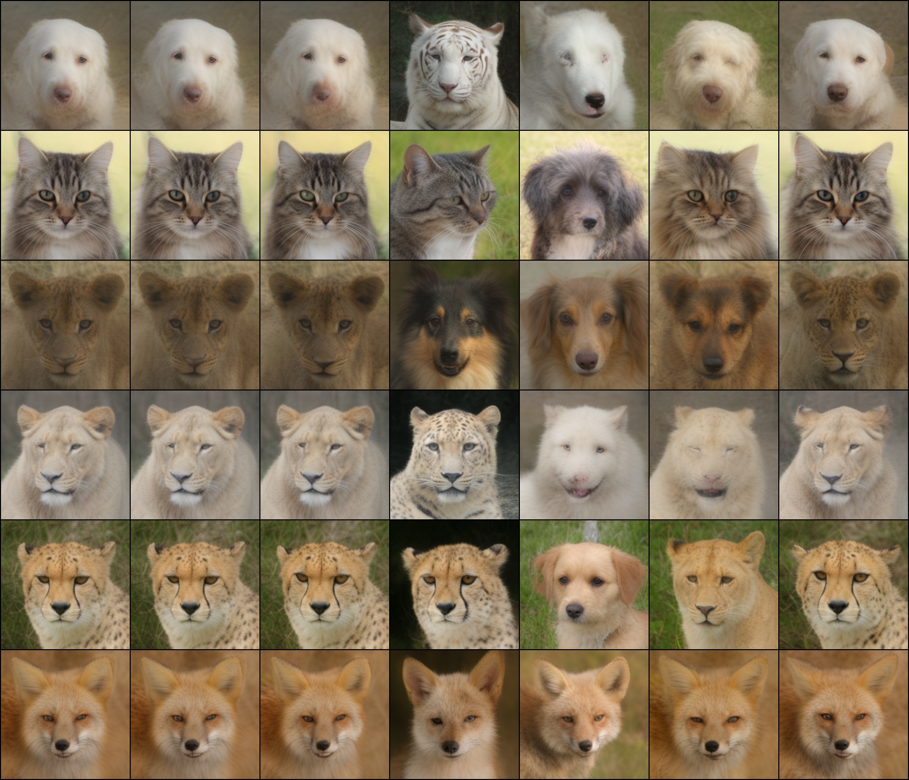
Figure 9: AFHQ latent space perturbation example. Each noise map of the images on the left is perturbed with a small noise in order to generate the images next to it, where in the second image from the left corresponds to the first diffusion step, i.e. $l=1$, and the first image from the right corresponds to perturbation of the last diffusion step, i.e. $l=L$. All the images are of size $256\times 256$.

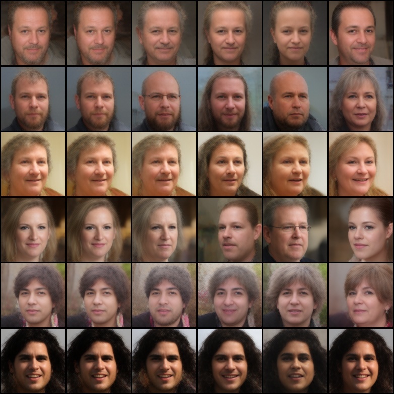
Figure 10: FFHQ latent space perturbation example. Each noise map of the images on the left is perturbed with a small noise in order to generate the images next to it, where in the second image from the left corresponds to the first diffusion step, i.e. $l=1$, and the first image from the right corresponds to perturbation of the last diffusion step, i.e. $l=L$. All the images are of size $128\times 128$.

C.3 Generation Results

We provide below additional generation results.

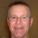
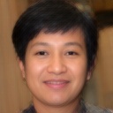
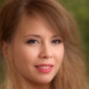
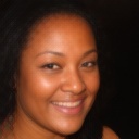
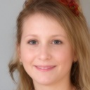
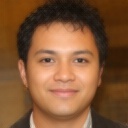
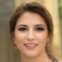
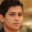
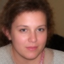
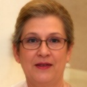
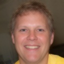
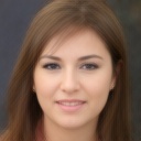
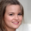
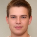
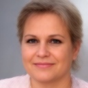
Figure 11: Unconditionally generated images using UDPM from the FFHQ128 dataset [20] using 6 network evaluations.

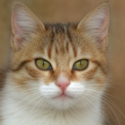
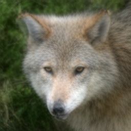
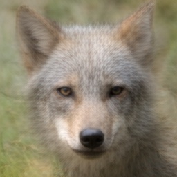
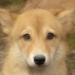
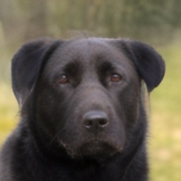
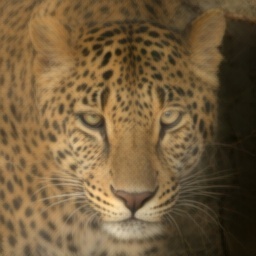
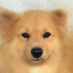
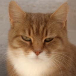
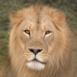
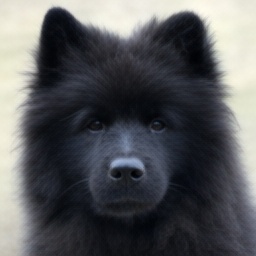
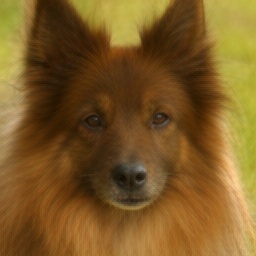
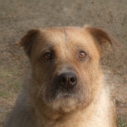
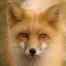
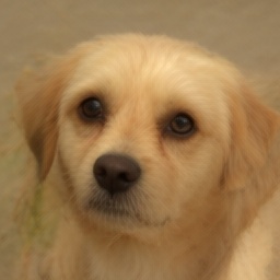
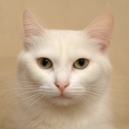
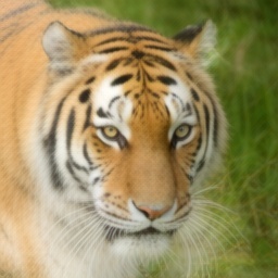
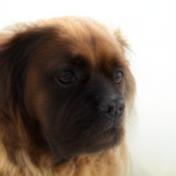
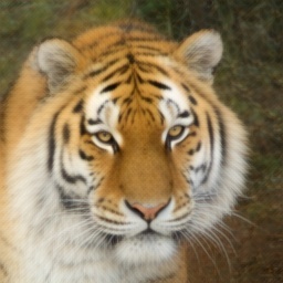
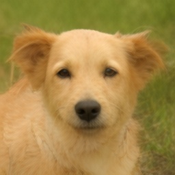
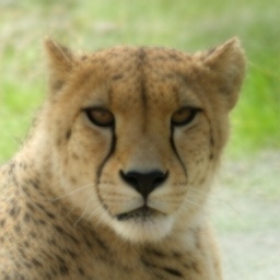
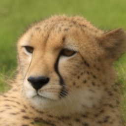
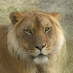
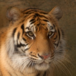
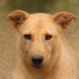
Figure 12: $256\times 256$ images generated using UDPM from the AFHQv2 dataset [20] using 7 network evaluations.

Figure 13: $64\times 64$ random images generated using UDPM from ImageNet dataset [29] using 5 network evaluations, with 1.5 classifier-free guidance scale.

Figure 14: $64\times 64$ random images generated using UDPM from ImageNet dataset [29] using 5 network evaluations, with 3.0 classifier-free guidance scale.

Figure 15: $64\times 64$ random images generated using UDPM from ImageNet dataset [29] using 5 network evaluations, with 3.0 classifier-free guidance scale.

References

- [1] Shady Abu-Hussein, Tom Tirer, and Raja Giryes. Adir: Adaptive diffusion for image reconstruction. 2022.
- [2] Omri Avrahami, Ohad Fried, and Dani Lischinski. Blended latent diffusion. arXiv preprint arXiv:2206.02779, 2022.
- [3] Omri Avrahami, Dani Lischinski, and Ohad Fried. Blended diffusion for text-driven editing of natural images. In Proceedings of the IEEE/CVF Conference on Computer Vision and Pattern Recognition, pages 18208–18218, 2022.
- [4] Arpit Bansal, Eitan Borgnia, Hong-Min Chu, Jie S. Li, Hamid Kazemi, Furong Huang, Micah Goldblum, Jonas Geiping, and Tom Goldstein. Cold diffusion: Inverting arbitrary image transforms without noise. arXiv:2208.09392, 2022.
- [5] Stanley H Chan, Xiran Wang, and Omar A Elgendy. Plug-and-play admm for image restoration: Fixed-point convergence and applications. IEEE Transactions on Computational Imaging, 3(1):84–98, 2016.
- [6] Ting Chen. On the importance of noise scheduling for diffusion models. arXiv preprint arXiv:2301.10972, 2023.
- [7] Yunjey Choi, Youngjung Uh, Jaejun Yoo, and Jung-Woo Ha. Stargan v2: Diverse image synthesis for multiple domains. In Proceedings of the IEEE/CVF conference on computer vision and pattern recognition, pages 8188–8197, 2020.
- [8] Hyungjin Chung, Eun Sun Lee, and Jong Chul Ye. Mr image denoising and super-resolution using regularized reverse diffusion. arXiv preprint arXiv:2203.12621, 2022.
- [9] Prafulla Dhariwal and Alexander Nichol. Diffusion models beat GANs on image synthesis. Advances in Neural Information Processing Systems, 34:8780–8794, 2021.
- [10] Tim Dockhorn, Arash Vahdat, and Karsten Kreis. Genie: Higher-order denoising diffusion solvers. arXiv preprint arXiv:2210.05475, 2022.
- [11] Shanghua Gao, Pan Zhou, Ming-Ming Cheng, and Shuicheng Yan. Masked diffusion transformer is a strong image synthesizer. arXiv preprint arXiv:2303.14389, 2023.
- [12] Giorgio Giannone, Didrik Nielsen, and Ole Winther. Few-shot diffusion models. 10.48550/ARXIV.2205.15463, 2022.
- [13] Florentin Guth, Simon Coste, Valentin De Bortoli, and Stephane Mallat. Wavelet score-based generative modeling, 2022.
- [14] Jonathan Ho, Ajay Jain, and Pieter Abbeel. Denoising diffusion probabilistic models. Advances in Neural Information Processing Systems, 33:6840–6851, 2020.
- [15] Jonathan Ho and Tim Salimans. Classifier-free diffusion guidance. arXiv preprint arXiv:2207.12598, 2022.
- [16] Shady Abu Hussein, Tom Tirer, and Raja Giryes. Correction filter for single image super-resolution: Robustifying off-the-shelf deep super-resolvers. In Proceedings of the IEEE/CVF Conference on Computer Vision and Pattern Recognition, pages 1428–1437, 2020.
- [17] Shady Abu Hussein, Tom Tirer, and Raja Giryes. Image-adaptive gan based reconstruction. In Proceedings of the AAAI Conference on Artificial Intelligence, volume 34, pages 3121–3129, 2020.
- [18] Zahra Kadkhodaie, Florentin Guth, Stéphane Mallat, and Eero P Simoncelli. Learning multi-scale local conditional probability models of images, 2023.
- [19] Tero Karras, Miika Aittala, Timo Aila, and Samuli Laine. Elucidating the design space of diffusion-based generative models. In NeurIPS, 2022.
- [20] Tero Karras, Samuli Laine, and Timo Aila. A style-based generator architecture for generative adversarial networks. In Proceedings of the IEEE/CVF conference on computer vision and pattern recognition, pages 4401–4410, 2019.
- [21] Bahjat Kawar, Shiran Zada, Oran Lang, Omer Tov, Huiwen Chang, Tali Dekel, Inbar Mosseri, and Michal Irani. Imagic: Text-based real image editing with diffusion models. arXiv preprint arXiv:2210.09276, 2022.
- [22] Diederik P Kingma and Jimmy Ba. Adam: A method for stochastic optimization. arXiv preprint arXiv:1412.6980, 2014.
- [23] Cheng Lu, Yuhao Zhou, Fan Bao, Jianfei Chen, Chongxuan Li, and Jun Zhu. Dpm-solver: A fast ode solver for diffusion probabilistic model sampling in around 10 steps. arXiv preprint arXiv:2206.00927, 2022.
- [24] Cheng Lu, Yuhao Zhou, Fan Bao, Jianfei Chen, Chongxuan Li, and Jun Zhu. Dpm-solver++: Fast solver for guided sampling of diffusion probabilistic models. arXiv preprint arXiv:2211.01095, 2022.
- [25] Alexander Quinn Nichol and Prafulla Dhariwal. Improved denoising diffusion probabilistic models. In International Conference on Machine Learning, pages 8162–8171. PMLR, 2021.
- [26] William Peebles and Saining Xie. Scalable diffusion models with transformers. arXiv preprint arXiv:2212.09748, 2022.
- [27] Alec Radford, Jong Wook Kim, Chris Hallacy, Aditya Ramesh, Gabriel Goh, Sandhini Agarwal, Girish Sastry, Amanda Askell, Pamela Mishkin, Jack Clark, et al. Learning transferable visual models from natural language supervision. In International Conference on Machine Learning, pages 8748–8763. PMLR, 2021.
- [28] Robin Rombach, Andreas Blattmann, Dominik Lorenz, Patrick Esser, and Björn Ommer. High-resolution image synthesis with latent diffusion models. In Proceedings of the IEEE/CVF Conference on Computer Vision and Pattern Recognition, pages 10684–10695, 2022.
- [29] Olga Russakovsky, Jia Deng, Hao Su, Jonathan Krause, Sanjeev Satheesh, Sean Ma, Zhiheng Huang, Andrej Karpathy, Aditya Khosla, Michael Bernstein, et al. Imagenet large scale visual recognition challenge. International journal of computer vision, 115(3):211–252, 2015.
- [30] Chitwan Saharia, Jonathan Ho, William Chan, Tim Salimans, David J Fleet, and Mohammad Norouzi. Image super-resolution via iterative refinement. IEEE Transactions on Pattern Analysis and Machine Intelligence, 2022.
- [31] Christoph Schuhmann, Romain Beaumont, Richard Vencu, Cade W Gordon, Ross Wightman, Mehdi Cherti, Theo Coombes, Aarush Katta, Clayton Mullis, Mitchell Wortsman, Patrick Schramowski, Srivatsa R Kundurthy, Katherine Crowson, Ludwig Schmidt, Robert Kaczmarczyk, and Jenia Jitsev. LAION-5b: An open large-scale dataset for training next generation image-text models. In Conference on Neural Information Processing Systems Datasets and Benchmarks Track, 2022.
- [32] Shelly Sheynin, Oron Ashual, Adam Polyak, Uriel Singer, Oran Gafni, Eliya Nachmani, and Yaniv Taigman. Knn-diffusion: Image generation via large-scale retrieval. arXiv:2204.02849, 2022.
- [33] Jascha Sohl-Dickstein, Eric Weiss, Niru Maheswaranathan, and Surya Ganguli. Deep unsupervised learning using nonequilibrium thermodynamics. In International Conference on Machine Learning, pages 2256–2265. PMLR, 2015.
- [34] Jiaming Song, Chenlin Meng, and Stefano Ermon. Denoising diffusion implicit models. In International Conference on Learning Representations, 2020.
- [35] Jiaming Song, Chenlin Meng, and Stefano Ermon. Denoising diffusion implicit models. In ICLR, 2022.
- [36] Jay Whang, Mauricio Delbracio, Hossein Talebi, Chitwan Saharia, Alexandros G Dimakis, and Peyman Milanfar. Deblurring via stochastic refinement. In Proceedings of the IEEE/CVF Conference on Computer Vision and Pattern Recognition, pages 16293–16303, 2022.
- [37] Fisher Yu, Ari Seff, Yinda Zhang, Shuran Song, Thomas Funkhouser, and Jianxiong Xiao. Lsun: Construction of a large-scale image dataset using deep learning with humans in the loop. arXiv preprint arXiv:1506.03365, 2015.
- [38] Richard Zhang, Phillip Isola, Alexei A Efros, Eli Shechtman, and Oliver Wang. The unreasonable effectiveness of deep features as a perceptual metric. In Proceedings of the IEEE conference on computer vision and pattern recognition, pages 586–595, 2018.