Fast Online Node Labeling for Very Large Graphs

Abstract

This paper studies the online node classification problem under a transductive learning setting. Current methods either invert a graph kernel matrix with $\mathcal{O}(n^{3})$ runtime and $\mathcal{O}(n^{2})$ space complexity or sample a large volume of random spanning trees, thus are difficult to scale to large graphs. In this work, we propose an improvement based on the online relaxation technique introduced by a series of works (Rakhlin et al., 2012; Rakhlin & Sridharan, 2015, 2017). We first prove an effective regret $\mathcal{O}(\sqrt{n^{1+\gamma}})$ when suitable parameterized graph kernels are chosen, then propose an approximate algorithm FastONL enjoying $\mathcal{O}(k\sqrt{n^{1+\gamma}})$ regret based on this relaxation. The key of FastONL is a generalized local push method that effectively approximates inverse matrix columns and applies to a series of popular kernels. Furthermore, the per-prediction cost is $\mathcal{O}(\operatorname{vol}\left(\mathcal{S}\right)\log 1/\epsilon)$ locally dependent on the graph with linear memory cost. Experiments show that our scalable method enjoys a better tradeoff between local and global consistency.

1 Introduction

This paper explores the online node labeling problem within a transductive learning framework. Specifically, we consider the scenario where multi-category node labels $\bm{y}_{t}$ enter online, and our goal is to predict future labels $\bm{y}_{t+1}$ under constraints imposed by an underlying graph. To illustrate this, consider the example of online product recommendations on platforms such as Amazon. At each time step $t$, the task is to recommend one of $k$ products to a user (node) based on their relationships (edges) with other users. The success of these recommendations is gauged by whether the user proceeds to purchase the recommended product. In this context, leveraging local information, such as recommendations from friends, becomes a viable strategy. However, this presents a significant challenge as we need to generate per-iteration predictions within microseconds while managing large-scale graphs comprising millions or even billions of nodes. Due to their computational complexity, traditional methods that require solving linear systems of order $\mathcal{O}\left(n^{3}\right)$ are ill-suited for this task where $n$ is the number of nodes. This issue is not only critical in web-spam classification (Herbster et al., 2008b), product recommendation (Ying et al., 2018), and community detection (Leung et al., 2009), but also permeates many other graph-based applications.

Previous studies in this area have fallen into two categories. The first involves sampling the spanning tree from the graph and then predicting labels via a weighted majority-like method (Herbster et al., 2008b; Cesa-Bianchi et al., 2009, 2013). Such methods require repeated spanning tree samplings and often suffer a large variance issue. The second family of methods designs a loss function and builds feature vectors from different graph kernels (Herbster et al., 2005; Herbster & Pontil, 2006; Herbster & Lever, 2009; Herbster et al., 2015; Gentile et al., 2013; Rakhlin & Sridharan, 2015, 2016b, 2017). These kernel-based methods can successfully capture the label smoothness of graphs but need to invert the graph kernel matrices, severely limiting their scalability.

Several classical and modern graph representation learning works (Zhu et al., 2003; Blum et al., 2004; Kipf & Welling, 2017) suggest that graph kernel-based methods are more effective in real-world applications. We focus on a significant line of work based on online relaxation (Rakhlin & Sridharan, 2015, 2016a, 2016b, 2017), which achieves linear time per-iteration cost. However, two challenges remain. First, the choice of the used graph kernel matrix affects performance, and it is unclear how to make this choice optimally and obtain an effective regret. Second, the previous relaxation method (Rakhlin & Sridharan, 2017) assumes that the inverse of the graph kernel matrix is readily available, which is not reasonable in practice. Note that a vanilla approach to computing a matrix inverse of a graph kernel involves $\mathcal{O}(n^{3})$ computational cost and $\mathcal{O}(n^{2})$ space complexity. Approximate matrix inverse techniques are required, but the regret guarantee for utilizing such schemes does not yet exist. The key question, then, is whether there exists an online node labeling method which accounts for the kernel matrix inversion, where the per-iteration cost is independent of the whole graph and the overall method is nearly-linear time.

In this paper, we propose such a solution by extending the online relaxation method (Rakhlin & Sridharan, 2015, 2016b, 2017, 2016a) via a fast local matrix inverse approximation method. Specifically, the inversion technique is based on the Approximate PageRank (APPR) method (Andersen et al., 2006), which is particularly effective and efficient when the magnitudes of these kernel vectors follow a power-law distribution, often found in real-world graphs. Our proposed Fast Online Node Labeling algorithm FastONL approximates the kernel matrix inverse via variants of APPR. Moreover, we compute an effective regret bound of $\mathcal{O}(k\sqrt{n^{1+\gamma}})$, which accounts for the matrix inversion steps. While we focus on static graphs, the method can naturally be extended to the dynamic graph setting.

Our contributions. 

• For the first time, we show that online relaxation-based methods with suitable graph kernel parametrization enjoy an effective regret when the graph is highly structured; specifically, the regret can be bounded by $\mathcal{O}(\sqrt{n^{1+\gamma}})$ if the graph Laplacian is regularized by $\mathcal{O}(n^{\gamma})$ for some $\gamma\in(0,1)$. This is generalized to several parameterized graph kernels.

• To overcome the $\mathcal{O}(n^{3})$ time and $\mathcal{O}(n^{2})$ space complexity of the large matrix inversion barrier, we consider the APPR approach, which gives a per-iteration cost of $\mathcal{O}(\operatorname{vol}\left(\mathcal{S}\right)\log(1/\epsilon))$. This locally linear bound is exponentially superior to the previous $\mathcal{O}(1/\epsilon)$ bound for general graphs (Andersen et al., 2006).

• On graphs between 1000 and 1M nodes, FastONL shows a better empirical tradeoff between local and global consistency. For a case study on the English Wikipedia graph with 6.2M nodes and 178M edges, we obtain a low error rate with a per-prediction run time of less than a second.

Our code and datasets have been provided as supplementary material and is publicly available at https://github.com/baojian/FastONL. All proofs have been postponed to the appendix.

2 Related Work

Online node labeling. 

Even binary labeling of graph nodes in the online learning setting can be challenging. A series of works on online learning over graphs is considered (Herbster et al., 2005; Herbster, 2008; Herbster et al., 2008b; Herbster & Lever, 2009; Herbster & Robinson, 2019; Herbster et al., 2021). Initially, Herbster et al. (2005) considered learning graph node labels using a perceptron-based algorithm, which iteratively projected a sequence of points over a closed convex set. This initial method already requires finding the pseudoinverse of the unnormalized Laplacian matrix. Moreover, the total mistakes is bounded by $4\Phi_{\mathcal{G}}(\bm{y})D_{\mathcal{G}}\operatorname{bal}(\bm{y})$ where $\Phi_{\mathcal{G}}$ is the graph cut, $D_{\mathcal{G}}$ is the diameter, and $\operatorname{bal}(\bm{y})$ is the label balance ratio. This mistake bound, which is distinct from the regret bound in this paper, vanishes when the label is imbalanced. Subsequent works, such as PUNCE (Herbster, 2008) and Seminorm (Herbster & Lever, 2009), also admitted mistake bounds. To remedy this issue, following works (Herbster & Pontil, 2006; Herbster et al., 2008a; Herbster, 2008) proposed different methods to avoid these large bounds. However, to the best of our knowledge, their effectiveness has not been validated on large-scale graphs. Additionally, it is unclear whether these methods can be effective under multi-category label settings.

The algorithms proposed in Herbster et al. (2008a); Herbster & Lever (2009); Cesa-Bianchi et al. (2009); Vitale et al. (2011); Cesa-Bianchi et al. (2013) accelerate per-prediction by working on trees and paths of the graph; see also (Gentile et al., 2013) for evolving graphs. However, the total time complexity of the proposed method is quadratic w.r.t the graph size. Additionally, Herbster et al. (2015) considered the setting of predicting a switching sequence over multiple graphs, and Gu & Han (2014) explored an online spectral learning framework. All these works fundamentally depend on the inverse of the graph Laplacian.

More generally, the problem of transductive learning on graphs has been extensively studied over past years (Ng et al., 2001; Zhou et al., 2003; Zhu et al., 2003; Ando & Zhang, 2006; Johnson & Zhang, 2007; El Alaoui et al., 2016; Kipf & Welling, 2017). Under batch transductive learning setting, the basic assumption is that nodes with same labels are well-clustered together. In this case, the quadratic form of the graph Laplacian kernel (2) or even $p$-Laplacian-based (El Alaoui et al., 2016; Fu et al., 2022) should be small. However, different from batch settings, this paper considers online learning settings based on kernel computations.

Personalized PageRank and approximation.  Personalized PageRank (PPR) as an important graph learning tool has been used in classic graph applications (Jeh & Widom, 2003; Andersen et al., 2008) and modern graph neural networks (Gasteiger et al., 2019; Bojchevski et al., 2020; Epasto et al., 2022) due its scalable approach to matrix inversion. The local push method has been proposed in a seminal work of Andersen et al. (2006) as an efficient and localized approach toward computing PPR vectors; it was later shown to be a variant of coordinate descent (Fountoulakis et al., 2019), and related to Gauss-Seidel iteration (Sun & Ye, 2021). This paper introduces a new variant of the local push to approximate many other graph kernel inverses.

3 Preliminaries

This section introduces notation and problem setup and presents the online relaxation method with surrogate loss.

3.1 Notations and problem formulation

Notations.  We consider an undirected weighted graph $\mathcal{G}=\left(\mathcal{V},\mathcal{E},\bm{W}\right)$ where $\mathcal{V}\triangleq\{1,2,\ldots,n\}$ is the set of nodes, $\mathcal{E}\subseteq\mathcal{V}\times\mathcal{V}$ is the set of $m=|\mathcal{E}|$ edges, and $\bm{W}\in{\mathbb{R}}_{+}^{n\times n}$ is the nonnegative weighted adjacency matrix where each edge $(u,v)\in\mathcal{E}$ has weight $W_{uv}>0$. The unnormalized and normalized graph Laplacian is defined as $\mathcal{{\bm{L}}}\triangleq\bm{D}-\bm{W}$ and $\bm{L}\triangleq{\bm{D}}^{-1/2}\mathcal{{\bm{L}}}{\bm{D}}^{-1/2}$, respectively. The set of neighbors of $u$ is denoted as $\mathcal{N}{(u)}\triangleq\{v:(u,v)\in\mathcal{E}\}$ and the degree $d_{u}=\left|\mathcal{N}{(u)}\right|$. The weighted degree matrix is defined as a diagonal matrix $\bm{D}$ where $D_{uu}=\sum_{v\in\mathcal{N}(u)}W_{uv}$. Following the work of Chung (1997), for $\mathcal{S}\subseteq\mathcal{V}$, the volume of $\mathcal{S}$ is defined as $\operatorname{vol}\left(\mathcal{S}\right)\triangleq\sum_{v\in\mathcal{S}}d_{v}$.

Given $k$ labels, each node $v$ has a label $y_{v}\in\{1,2,\ldots,k,\}$. For convenience, we use the binary form ${\bm{y}}_{t}\in\{{\bm{e}}_{1},{\bm{e}}_{2},\ldots,{\bm{e}}_{k}\}=:\mathcal{Y}$ where $\bm{e}_{i}$ is the one-hot encoding vector. $\bm{X}_{:,i}\in\mathbb{R}^{n}$ is the $i$-th column vector of matrix $\bm{X}\in{\mathbb{R}}^{n\times n}$ and $\bm{X}_{i,:}\in\mathbb{R}^{n}$ is the transpose of $i$-th row vector of $\bm{X}$. The support of $\bm{x}\in\mathbb{R}^{n}$ is $\operatorname{supp}\left(\bm{x}\right)\triangleq\{v:x_{v}\neq 0,v\in\mathcal{V}\}$. The trace of a square matrix $\bm{M}$ is defined as $\operatorname{tr}\left(\bm{M}\right)=\sum_{i=1}^{n}m_{ii}$ where $m_{ii}$ is the $i$-th diagonal. For a symmetric matrix $\bm{M}$, denote $\lambda(\bm{M})$ as the eigenvalue function of $\bm{M}$.

Table 1: The parameterized graph kernel matrices with their basic kernel presentation

ID	$\bm{K}_{\beta}^{-1}$	$\alpha$	Basic Kernel Presentation	Paper
1	$\mathcal{L}$	$\frac{\lambda}{n}$	$\bm{M}_{\lambda,\beta}=2\lambda\bm{X}_{\mathcal{L}}$	(Rakhlin & Sridharan, 2017)
2	${\bm{L}}$	$\frac{\lambda}{n+\lambda}$	$\bm{M}_{\lambda,\beta}=2n{\bm{D}}^{-1/2}\bm{X}_{\bm{L}}{\bm{D}}^{1/2}$	(Rakhlin & Sridharan, 2017)
3	$\bm{I}-\beta\bm{D}^{-1/2}\bm{W}\bm{D}^{-1/2}$	$\frac{n+\lambda-\beta n}{n+\lambda}$	$\bm{M}_{\lambda,\beta}=\frac{2\lambda n}{n+\lambda-\beta n}{\bm{D}}^{-1/2}\bm{X}_{\bm{L}}{\bm{D}}^{1/2}$	(Zhou et al., 2003)
4	$\beta{\bm{I}}+{\bm{S}}^{-1/2}\mathcal{\bm{L}}{\bm{S}}^{-1/2}$	$\frac{n\beta+\lambda}{n}$	$\bm{M}_{\lambda,\beta}=2\lambda{\bm{S}}^{-1/2}\bm{X}_{\mathcal{L}}{\bm{S}}^{1/2}$	(Johnson & Zhang, 2008)
5	${\bm{S}}^{-1/2}(\beta{\bm{I}}+\mathcal{\bm{L}}){\bm{S}}^{-1/2}$	$2\lambda$	$\bm{M}_{\lambda,\beta}=\big{(}\frac{\bm{S}^{1/2}}{4n\lambda}+\frac{\beta\bm{S}^{-1/2}}{4\lambda^{2}}\big{)}^{-1}\bm{X}_{\mathcal{L}}{\bm{S}}^{1/2}$	(Johnson & Zhang, 2007)
6	$\mathcal{\bm{L}}+b\cdot\bm{1}\bm{1}^{\top}+\beta\bm{I}$	$\beta+\frac{\lambda}{n}$	$\bm{M}_{\lambda,\beta}=2\lambda\bm{X}_{\mathcal{L}}\big{(}\bm{I}-\frac{b\bm{1}\bm{1}^{\top}}{\alpha+nb}\big{)}$	(Herbster et al., 2005)

Problem formulation.  This paper considers the following online learning paradigm on $\mathcal{G}$: At each time $t=1,2,\ldots,n$, a learner picks a node $v$ and makes a prediction $\hat{\bm{y}}_{v}\in\mathcal{Y}$. The true label $\bm{y}_{v}$ is revealed by the adversary with a corresponding 0-1 loss $\ell(\hat{\bm{y}}_{v},\bm{y}_{v})=1-{\bm{y}}_{v}^{\top}\hat{\bm{y}}_{v}$ back to the learner. The goal is to design an algorithm, so the learner makes as few mistakes as possible. Denote a prediction of $\mathcal{V}$ as $\widehat{\bm{Y}}=\left[\hat{\bm{y}}_{1},\hat{\bm{y}}_{2},\ldots,\hat{\bm{y}}_{n}\right]\in\mathcal{F}$ and true label configuration as ${\bm{Y}}=\left[{\bm{y}}_{1},{\bm{y}}_{2},\ldots,{\bm{y}}_{n}\right]\in\mathcal{F}$ from the allowed label configurations $\mathcal{F}\in\left\{\bm{F}\in\{0,1\}^{k\times n}:{\bm{F}}_{:,j}^{\top}\cdot{\bm{1}}=1,\forall j\in\mathcal{V}\right\}$. Without further restrictions, the adversary could always select a $\bm{Y}$ so that the learner makes the maximum ($n$) mistakes by always providing $\bm{y}_{v}\neq\hat{\bm{y}}_{v}$. Therefore, to have learnability, often the set $\mathcal{F}$ is restricted to capture label smoothness (Blum & Mitchell, 1998; Blum & Chawla, 2001; Zhu et al., 2003; Zhou et al., 2003; Blum et al., 2004). Formally, given an algorithm $\mathcal{A}$, the learner’s goal is to minimize the regret defined as

$$\mathop{\operatorname{Reg}}_{\widehat{\bm{Y}}\sim\mathcal{A}}:=\sum_{t=1}^{n}\ell(\hat{\bm{y}}_{t},\bm{y}_{t})-\min_{\bm{F}\in\mathcal{F}_{\lambda,\beta}}\sum_{t=1}^{n}\ell(\bm{F}_{:,t},\bm{y}_{t}),$$ (1)

where

$$\mathcal{F}_{\lambda,\beta}=\left\{\bm{F}\in\mathcal{F}:\sum_{i=1}^{k}{{\bm{F}}_{i,:}}^{\top}{\bm{K}}_{\beta}^{-1}{\bm{F}}_{i,:}\leq\lambda\right\},$$ (2)

and $\bm{K}_{\beta}$ is a positive definite kernel parameterized by $\beta$, and $\lambda$ is a label smoothing parameter controlling the range of allowed label configurations. For example, assume $\bm{K}_{\beta}^{-1}=\bm{D}-\bm{W}$ for a unit weight graph; then if $\lambda=1$, $\mathbf{y}_{i}=\mathbf{y}_{j}$ whenever $(i,j)\in\mathcal{E}$ for all $\mathbf{Y}\in\mathcal{F}$; clearly in this case the labeling is learnable. On the other hand, if $\lambda>n$, then $\mathbf{Y}$ can be any labeling and is not learnable. If $\ell$ is convex with a closed convex set $\mathcal{F}$, typical online convex optimization methods such as online gradient descent or Follow-The-Regularized-Leader could provide sublinear regret (Shalev-Shwartz et al., 2012; Hazan et al., 2016) for minimizing the regret (1). However, when $\ell$ is the 0-1 loss, the combinatorial nature of $\mathcal{F}$ makes directly applying these methods difficult. Inspired by Rakhlin & Sridharan (2017), we propose the following convex relaxation of $\mathcal{F}_{\lambda,\beta}$ to

$$\bar{\mathcal{F}}_{\lambda,\beta}=\left\{{\bm{F}}\in\mathbb{R}^{k\times n}:\sum_{i=1}^{k}{\bm{F}}_{i,:}^{\top}\bm{M}_{\lambda,\beta}{\bm{F}}_{i,:}\leq 1\right\},$$

where $\mathcal{F}_{\lambda,\beta}\subseteq\bar{\mathcal{F}}_{\lambda,\beta}$ and the regularized kernel matrix is

$$\bm{M}_{\lambda,\beta}=\left(\frac{{\bm{K}}_{\beta}^{-1}}{2\lambda}+\frac{\bm{I}_{n}}{2n}\right)^{-1}.$$ (3)

3.2 Online relaxation and surrogate loss

Algorithm 1 Relaxation$(\mathcal{G},\lambda,D)$(Rakhlin & Sridharan)

1:  Compute $\bm{M}=\bm{M}_{\lambda,\beta}$

2:  $T_{1}=\operatorname{tr}\left(\bm{M}\right),A_{1}=0,\bm{G}=[\bm{0},\ldots,\bm{0}]\in\mathbb{R}^{k\times n}$

3:  for $t=1,\ldots,n$ do

4:     $\bm{\psi}_{t}=-\bm{G}\bm{M}_{:,t}/\sqrt{A_{t}+D^{2}\cdot T_{t}}$

5:     Predict $\hat{\bm{y}}_{t}\sim\bm{q}_{t}(\bm{\psi}_{t})$, $\bm{\nabla}_{t}=\bm{\nabla}\phi_{\bm{\psi}_{t}}(\cdot,\bm{y})$

6:     Update $\bm{G}_{:,t}=\bm{\nabla}_{t}$

7:     $A_{t+1}=A_{t}+2\bm{\nabla}_{t}^{\top}\bm{G}\bm{M}_{:,t}+m_{tt}\cdot\|\bm{\nabla}_{t}\|_{2}^{2}$

8:     $T_{t+1}=T_{t}-m_{tt}$

9:  end for

In the online relaxation framework (Alg.1), a key step of prediction node $t$ is to choose a suitable $\bm{\psi}_{t}$ strategy so that the regret defined in (1) can be bounded. Specifically, the prediction $\hat{\bm{y}}_{t}$ is randomly generated according to distribution $\bm{q}_{t}(\bm{\psi}_{t})$ where the score $\bm{\psi}_{t}\in\mathbb{R}^{k}$ is a scaling of $-\sum_{i<t}\bm{\nabla}_{i}M_{i,t}$, computed in an online fashion. The distribution, $q_{i}=\max(\psi_{i}-\tau,0)$ for the choice of $\tau$ such that $\sum_{i=1}^{k}q_{i}=1$. This technique corresponds to minimizing the surrogate convex loss

$$\phi_{\bm{\psi}}(\bm{g},\bm{y})=\begin{cases}\frac{1+\max_{r:\bm{e}_{r}\neq\bm{y}}\left\{\bm{g}^{\top}\bm{e}_{r}-\bm{g}^{\top}\bm{y}\right\}}{1+1/|S(\bm{\psi})|}&\bm{y}\notin{S}(\bm{\psi})\\ 1-\bm{g}^{\top}\bm{y}+\frac{\bm{g}^{\top}\bm{1}_{S(\bm{\psi})}-1}{|S(\bm{\psi})|}&\bm{y}\in S(\bm{\psi})\end{cases}$$ (4)

where $S\left(\bm{\psi}\right)$ is the support of $\bm{\psi}$, and $\bm{\nabla}_{t}$ is the gradient of $\phi(\cdot,\bm{y})$ of the first variable. Specifically, $y_{t}\notin S(\bm{\psi})$ means the learner receives loss $\phi_{\bm{\psi}}(\bm{g},\bm{y})\geq 1$. Note that the per-iteration cost of Alg.1 is $\mathcal{O}(kn)$ once the $\bm{\psi}_{t}$ is computed.

We now define an admissible relaxation function.

Definition 3.1 (Admissible function (Rakhlin et al., 2012)).

Let $\bm{\nabla}_{i}\in\mathbb{R}^{k}$, $\|\bm{\nabla}_{i}\|_{2}\leq D$ for some $D>0$. A real-valued function $\operatorname{Rel}({\bm{\nabla}}_{1:t})$ is said to be admissible if, for all $t\in\mathcal{V}$, it satisfies recursive inequalities

$$\inf_{\bm{\psi}_{t}\in\mathbb{R}^{k}}\sup_{\|\bm{\nabla}_{t}\|_{2}\leq D}\left\{\bm{\nabla}_{t}^{\top}\bm{\psi}_{t}+\operatorname{Rel}({\bm{\nabla}}_{1:t})\right\}\leq\operatorname{Rel}({\bm{\nabla}}_{1:t-1}),$$

with $\operatorname{Rel}(\bm{\nabla}_{1:n})\geq-\inf_{\bm{F}\in\mathcal{F}_{\lambda,\beta}}\sum_{t=1}^{n}\bm{\nabla}_{t}^{\top}\bm{F}_{:,t}$.

It was shown in Rakhlin et al. (2012) (and later (Rakhlin & Sridharan, 2015, 2016b, 2017)) that if there exists an admissible function $\operatorname{Rel}$ for some $\bm{\psi}_{t}$, then the regret of Alg.1 is upper bounded by $\operatorname{Rel}(\emptyset)=\sqrt{D\cdot\operatorname{tr}\left(\bm{M}\right)}$, providing an upper bound of the regret. Here $\bm{M}$ is either $(\tfrac{\mathcal{L}}{2\lambda}+\tfrac{\bm{I}}{2n})^{-1}$ or $(\tfrac{\bm{L}}{2\lambda}+\tfrac{\bm{I}}{2n})^{-1}$ for the binary case. Note that in both cases, since $\lambda_{\max}(\bm{M})\leq n$, then in the worst case, the regret could be $\mathcal{O}(n)$ (vanishing in general). Thus, two questions remain.

1. Does there exist $\bm{K}_{\beta}^{-1}$ that not only captures label smoothness but also has regret smaller than $\mathcal{O}(n)$?

2. How do we reconcile the kernel computation overhead $\mathcal{O}(n^{3})$ but still provide an effective regret bound?

These two main problems motivate us to study this online relaxation framework further. Sec. 4 answers the second question by showing that solving many popular kernel matrices is equivalent to solving two basic kernel matrices, and we explore local approximate methods for both. We then answer the first question in Sec. 5 by proving effective bounds when the parameterized kernel matrix is computed exactly or approximated.

4 Local approximation of kernel $\bm{M}_{\lambda,\beta}$

Section 4.1 presents how popular kernels can be evaluated from simple transformations of the inverse approximations computed via FIFOPush, whose convergence is described in Section 4.2.

4.1 Basic kernel presentations of $\bm{M}_{\lambda,\beta}$

The regularized kernel matrix is defined in (3) for various instances of $\bm{K}_{\beta}^{-1}$ as listed in Tab. 1. As shown in the table, a key observation is that several existing online labeling methods involve the inverse of two basic kernel forms. We present this in Thm. 4.

Theorem 4.1.

Let $\bm{K}_{\beta}^{-1}$ be the inverse of the symmetric positive definite kernel matrix defined in Tab. 1. Then $\bm{M}_{\lambda,\beta}$ can be decomposed into $\bm{M}_{\lambda,\beta}=a\bm{A}^{-1}\bm{X}\bm{B}$, which is easily computed once $\bm{X}$ available. $\bm{X}$ represents two basic kernels

$$\bm{X}_{\mathcal{L}}=\left(\alpha\bm{I}+\mathcal{L}\right)^{-1},\quad\bm{X}_{\bm{L}}=\alpha\left(\bm{I}-(1-\alpha)\bm{W}\bm{D}^{-1}\right)^{-1}$$

corresponding to the inverse of variant matrices of $\mathcal{L}$ and $\bm{L}$, respectively.

In Tab. 1, the column “Basic Kernel Presentation” shows how $\bm{M}_{\lambda,\beta}$ can then be efficiently computed from either $\bm{X}_{\bm{L}}$ or $\bm{X}_{\mathcal{L}}$, using minimal post-processing overhead. As in the online relaxation framework, for any time $t$ of node $v_{t}$, it requires to access the $v_{t}$-th column of $\bm{M}_{\lambda,\beta}$. Therefore, we need to solve the following two basic equations

$$\text{Type-}\mathcal{L}\text{:\quad}{\bm{x}}_{v_{t}} =\bm{X}_{\mathcal{L}}{\bm{e}}_{v_{t}},$$ (5)

$$\text{Type-}\bm{L}\text{:\quad}{\bm{x}}_{v_{t}} =\bm{X}_{\bm{L}}{\bm{e}}_{v_{t}}.$$ (6)

For the second case, note ${\bm{x}}_{v_{t}}=\bm{X}_{\bm{L}}{\bm{e}}_{v_{t}}$ gives the Personalized PageRank Vector (PPV) (Page et al., 1999; Jeh & Widom, 2003). For example, using $\alpha=\tfrac{n}{n+\kappa}$, we compute $\bm{M}_{\lambda,\beta}=2n{\bm{D}}^{-1/2}\bm{X}_{\bm{L}}{\bm{D}}^{1/2}$ where $\bm{X}_{\bm{L}}$ is the Personalized PageRank matrix (See the second row of Tab. 1). We now discuss the inversion for computing $\bm{X}_{\bm{L}}$ and $\bm{X}_{\mathcal{L}}$.

Algorithm 2 $\textsc{FIFOPush}(\mathcal{G},\epsilon,\alpha,s)$

1:  $\bm{r}=\begin{cases}\text{Type-}{\mathcal{L}}:\tfrac{\bm{e}_{s}}{\alpha}\\ \text{Type-}{\bm{L}}:\bm{e}_{s}\end{cases}$

2:  $\bm{x}=\bm{0},\mathcal{Q}=[s]$

3:  while $\mathcal{Q}\neq\emptyset$ do

4:     $u=\mathcal{Q}\text{.pop()}$

5:     if $r_{u}<\epsilon\cdot d_{u}$ then

6:        continue

7:     end if

8:     $x_{u}=\begin{cases}\text{Type-}{\mathcal{L}}\text{: }x_{u}+\tfrac{\alpha r_{u}}{\alpha+D_{u}}\\ \text{Type-}{\bm{L}}\text{: }x_{u}+\alpha r_{u}\end{cases}$

9:     for $v\in\mathcal{N}(u)$ do

10:        $r_{v}=\begin{cases}\text{Type-${\mathcal{L}}$: }r_{v}+\tfrac{r_{u}}{\alpha+D_{u}}\cdot w_{uv}\\ \text{Type-${\bm{L}}$: }r_{v}+\frac{(1-\alpha)r_{u}}{D_{u}}\cdot w_{uv}\end{cases}$

11:        if $v\notin\mathcal{Q}$ then

12:           $\mathcal{Q}\text{.push}(v)$

13:        end if

14:     end for

15:     $r_{u}=0$

16:  end while

17:  Return $\bm{x},\bm{r}$

Before introducing the FIFOPush inversion method, let us consider the more commonly used power iteration for matrix inversion. $\bm{M}_{\lambda,\beta}$ can be approximated by a series of matrix multiplications. Take $\bm{K}_{\beta}^{-1}=\bm{I}-\bm{D}^{-1/2}\bm{W}\bm{D}^{-1/2}$ as an example. Then a truncated power iteration gives

$$\bm{M}_{\lambda,\beta} \approx\frac{2n\lambda}{n+\lambda}\sum_{i=0}^{p}\Big{(}\frac{n}{n+\lambda}\bm{D}^{-1/2}\bm{W}\bm{D}^{-1/2}\Big{)}^{i}$$ (7)

assuming that $\|\tfrac{n}{n+\lambda}\bm{D}^{-1/2}\bm{W}\bm{D}^{-1/2}\|_{2}<1$ (See Lemma 2.3.3 of Golub & Van Loan (2013)). When $p$ is small, this method often produces a reasonable and efficient approximation of $\bm{M}_{\lambda,\beta}$, and is especially efficient if $\bm{W}$ is sparse. However, as $p$ gets large, the intermediate iterates quickly become dense matrices, creating challenges for online learning algorithms where the per-kernel vector operator is preferred ( See also Fig. 15 on real-world graphs ). Thus, the situation is even worse when we only need to access one column at each time $t$ under the online learning setting.

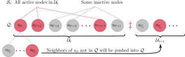
Figure 1: The illustration of $t$-th epoch of FIFOPush. At the initial of $t$-th epoch, $\mathcal{Q}=[u_{t^{\prime}},\ldots,u_{t^{\prime}+i}]$ contains all active nodes (red) $\mathcal{S}_{t}$ and part of inactive nodes (gray). After the first active node $u_{t^{\prime}}$ has been processed, the neighbors of $u_{t^{\prime}}$ that are not in $\mathcal{Q}$ will be pushed into $\mathcal{Q}$ for next $(t+1)$-th epoch. ${\color[rgb]{1,0,0}{\ddagger}}$ is a dummy node to mark the end of an epoch.

For these reasons, we introduce FIFOPush (Alg. 2), which reduces to the well-known APPR algorithm (Andersen et al., 2006) when the goal is to approximate $\bm{X}_{\bm{L}}$. Specifically, it is a local push method for solving either (5) or (6) based on First-In-First-Out (FIFO) queue. Each node $u_{t}\in\mathcal{S}_{t}$ is either active, i.e., $r_{u_{t}}\geq\epsilon d_{u_{t}}$, or inactive otherwise. As illustrated in Fig. 1, at a higher level, it maintains a set of nonzero residual nodes $\mathcal{U}_{t}$ and active nodes $\mathcal{S}_{t}\subseteq\mathcal{U}_{t}$ in each epoch $t$. FIFOPush updates the solution column $\bm{x}$ and residual $\bm{r}$ (corresponding to the “gradient”) by shifting mass from a high residual node (an active node) to its neighboring nodes in $\bm{x}$ and $\bm{r}$. This continues until all residual nodes are smaller than a tolerance $\epsilon$. This method essentially retains the linear invariant property introduced in Appendix A.2.

4.2 Local linear convergence of FIFOPush

(a) Labeled Karate

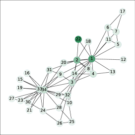
(b) $\bm{x}_{22,\epsilon}$ on $\mathcal{G}$

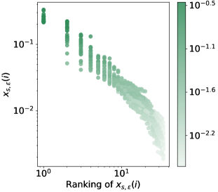
(c) Power law of $\bm{X}_{\epsilon}$

Figure 2: Power law distribution of $|(\bm{X}_{\bm{L}}\bm{e}_{s})_{i}|$ on Karate graph (Girvan & Newman, 2002). (a) The Karate contains 34 nodes and 78 edges forming four communities ($w_{uv}$ is the 2-dimensional Euclidean distance.); (b) We run FIFOPush$(\mathcal{G},\epsilon,\alpha,s)$ on $s=22$ with $\alpha=0.2$ and $\epsilon=10^{-12}$. Neighbors of $s=22$ have large magnitudes of $\bm{x}_{s}$; (c) The power law distribution of entries of $\bm{x}_{s}$ for all 34 nodes.

For calculating $\bm{X}_{\bm{L}}$, Andersen et al. showed that FIFOPush gives a time complexity $\mathcal{O}(\tfrac{1}{\alpha\epsilon})$ for precision level $\epsilon>0$. This bound is local sublinear, meaning the bound is locally dependent of $\mathcal{G}$ and sublinear to the precision $\epsilon$. Moreover, the rate’s independence on $\mathcal{G}$ is a key advantage of FIFOPush over other numerical methods such as Power Iteration, which is similar to FIFOPush (Wu et al., 2021) when $\epsilon<\mathcal{O}(m^{-1})$ (recall $m=|\mathcal{E}|$). Specifically, the Power Iteration typically needs $\mathcal{O}(\tfrac{m}{\alpha}\log\tfrac{1}{\epsilon})$ operations. However, when $m$ is large, and $\epsilon$ is very small, the advantage of the local sublinear bound is lost, and the time complexity bound is not optimal.

It is natural to ask whether any method achieves a locally dependent and logarithmically related bound to $\epsilon$. We answer this question positively. Specifically, we notice that in most real-world sparse graphs, the columns of $\bm{X}$ have magnitudes following a power law distribution (See Karate graph in Fig. 2, real-world graphs shown in Fig. 17 and 18 for $\bm{X}_{\bm{L}}$ and $\bm{X}_{\mathcal{L}}$, respectively.), suggesting that local approximations are sufficient in computing high fidelity approximate inverses. Note that this greatly improves computational complexity and preserves memory locality, reducing graph access time for large-scale graphs.

We now provide our local linear and graph independent complexity bound. Denote the estimation matrix $\bm{X}_{\epsilon}=\left[\bm{x}_{1,\epsilon},\ldots,\bm{x}_{n,\epsilon}\right]$ and the residual matrix $\bm{R}_{\epsilon}=\left[\bm{r}_{1,\epsilon},\ldots,\bm{r}_{n,\epsilon}\right]$ where $(\bm{x}_{s,\epsilon},\bm{r}_{s,\epsilon})=\textsc{FIFOPush}(\mathcal{G},\epsilon,\alpha,s)$ for all $s\in\mathcal{V}$. Denote $\mathcal{I}_{t}=\operatorname{supp}\left(\bm{r}_{t}\right)$ as the support of residual after $t$-th epoch, and $\mathcal{S}_{t}$ as the set of active nodes.

Theorem 4.2 (Local linear convergence of FIFOPush for $\bm{X}_{\bm{L}}$).

Let $\bm{x}_{s}=\bm{X}_{\bm{L}}\bm{e}_{s}$. Denote $T$ as the total epochs executed by FIFOPush, and $\mathcal{S}_{t}:=\{v:r_{t}(v)\geq\epsilon\cdot d_{v},v\in\mathcal{I}_{t}\}$ as the set of active nodes in $t$-th epoch. Then, the total operations of $\textsc{FIFOPush}(\mathcal{G},\epsilon,\alpha,s)$ is dominated by

$$R_{T}:=\sum_{t=1}^{T}\sum_{u_{t}\in{\mathcal{S}}_{t}}d_{u_{t}}\leq\frac{\operatorname{vol}\left(\mathcal{S}_{1:T}\right)}{\alpha\cdot\eta_{1:T}}\log\left(\frac{C_{\alpha,T}}{\epsilon}\right),$$ (8)

where $\operatorname{vol}\left(\mathcal{S}_{1:T}\right)=\sum_{t=1}^{T}\operatorname{vol}\left(\mathcal{S}_{t}\right)/T$ is the average volume of $\mathcal{S}_{t}$. Additionally, $\eta_{1:T}=\sum_{t=1}^{T}\eta_{t}/T$ is the average of local convergence factors $\eta_{t}\triangleq\sum_{u\in\mathcal{S}_{t}}d_{u}/\sum_{v\in\mathcal{I}_{t}}d_{v}$, and $C_{\alpha,T}=1/(\sum_{v\in\mathcal{I}_{T}}(1-\alpha)d_{u}w_{uv}/D_{u})$. For $s,i\in\mathcal{V}$, we have $\bm{x}_{s}=\bm{x}_{s,\epsilon}+\bm{X}_{\bm{L}}\bm{r}_{s,\epsilon},r_{s,\epsilon}(i)\leq[0,\epsilon d_{i})$.

Thm. 4.2 provides a local linear convergence of FIFOPush where both $\operatorname{vol}\left(\mathcal{S}_{1:T}\right)$ and ${\eta}_{1:T}$ are locally dependent on $\mathcal{G}$, $\alpha$, and $\epsilon$. For unweighted $\mathcal{G}$, the bound in (8) can be simplified as $\tfrac{\operatorname{vol}\left(\mathcal{S}_{1:T}\right)}{\alpha\cdot\eta_{1:T}}\log\tfrac{1}{\epsilon(1-\alpha)|\mathcal{I}_{T}|}$. The key of Thm. 4.2 is to evaluate $\operatorname{vol}\left(\mathcal{S}_{1:T}\right)$ and $\eta_{1:T}$. To estimate $\operatorname{vol}\left(\mathcal{S}_{1:T}\right)$, since each active node appears at most $T$ times and at least once in all $T$ epochs, after FIFOPush terminates, we have

$$\frac{\operatorname{vol}\left(\operatorname{supp}\left(\bm{x}_{s,\epsilon}\right)\right)}{T}\leq\operatorname{vol}\left(\mathcal{S}_{1:T}\right)\leq\operatorname{vol}\left(\operatorname{supp}\left(\bm{x}_{s,\epsilon}\right)\right),$$

where for $\alpha$ and $\epsilon$ such that $\mathcal{O}(|\operatorname{supp}\left(\bm{x}_{s,\epsilon}\right)|)\ll n$ means $\mathcal{O}(\operatorname{vol}\left(\operatorname{supp}\left(\bm{x}_{s,\epsilon}\right)\right))\ll m$ in expectation. More importantly, compared with $\mathcal{O}(1/\alpha\epsilon)$ of Andersen et al. (2006), Thm. 4.2 provides a better bound when $\epsilon\leq\mathcal{O}(m^{-1})$. The work of Fountoulakis et al. (2019) shows APPR is equivalent to the coordinate descent method, and the total time complexity is comparable to $\tilde{\mathcal{O}}(\tfrac{1}{\alpha\epsilon})$.

The average of the linear convergence factor $\eta_{1:T}$ is always $>0$ by noticing that at least one active node is processed in each epoch. One can find more quantitative discussion in Appendix A.2. The above theorem is a refinement of (Wu et al., 2021) where $\mathcal{O}(m\log\frac{1}{\epsilon})$ is obtained (only effective when $\epsilon<1/2m$). However, our proof shows that obtaining $m$ independent bound is possible by showing that local magnitudes are reduced by a constant factor. The above theorem gives a way to approximate $\bm{M}_{\lambda,\beta}$, and we will build an approximate online algorithm based on FIFOPush. We close this section by introducing our local linear convergence for $\bm{X}_{\mathcal{L}}\bm{e}_{s}$ as the following.

Theorem 4.3 (Local convergence of FIFOPush for $\bm{X}_{\mathcal{L}}$).

Let $\bm{x}_{s}=\bm{X}_{\mathcal{L}}\bm{e}_{s}$ and run Aglo. 2 for $\bm{X}_{\mathcal{L}}$. For $s,i\in\mathcal{V}$, we have $\bm{x}_{s}=\bm{x}_{s,\epsilon}+\alpha\bm{X}_{\mathcal{L}}\bm{r}_{s,\epsilon},\text{ with }r_{s,\epsilon}(i)\leq[0,\epsilon d_{i}),\forall i\in\mathcal{V}$. The main operations of FIFOPush for $\bm{X}_{\mathcal{L}}$ is bounded as

$$R_{T}\leq\frac{\operatorname{vol}\left(\mathcal{S}_{1:T}\right)(\alpha+D_{\max})}{\alpha\cdot\eta_{1:T}}\log\left(\frac{C_{\alpha,T}}{\epsilon}\right),$$ (9)

where $\operatorname{vol}\left(\mathcal{S}_{1:T}\right)$ and $\eta_{1:T}$ are the same as in Thm. 4.2, $\eta_{t}\triangleq\tfrac{\sum_{u\in\mathcal{S}_{t}}d_{u}/(\alpha+D_{u})}{\sum_{v\in\mathcal{I}_{t}}d_{v}/(\alpha+D_{v})}$, $C_{\alpha,T}=1/\sum_{v\in\mathcal{I}_{T}}\frac{d_{u}w_{uv}}{\alpha+D_{u}}$, and $D_{\max}=\max_{v\in\operatorname{supp}\left(\bm{x}_{s,\epsilon}\right)}D_{v}$.

Remark 4.4.

We obtain a similar local linear convergence for solving $\bm{X}_{\mathcal{L}}$ by FIFOPush. The additional factor $(\alpha+D_{\max})$ appears in Equ. (9) due to the upper bound of the maximal eigenvalue of $\mathcal{L}$.

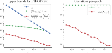
Figure 3: The bounds comparison of $R_{T}$. To see if there is a true advantage of our bound, we compare two bounds of FIFOPush, $\mathcal{O}(\tfrac{1}{\alpha\epsilon})$ (Andersen et al., 2006) and $\mathcal{O}(m\frac{m}{\alpha}\log\frac{1}{\epsilon m}+m)$ (Wu et al., 2021) with Ours. Each vertical line with its left part is when $\epsilon$ satisfies Cor. 10

5 Fast Online Node Labelling: FastONL

This section shows how we can obtain a meaningful regret using parameterized graph kernels for the original online relaxation method. We then design approximated methods based on FIFOPush.

5.1 Regret analysis for online relaxation method

As previously discussed, simply applying $\bm{M}_{\lambda,\beta}^{-1}=\mathcal{L}$ or $\bm{L}$ will not yield a meaningful regret as the maximal eigenvalue of $\bm{M}_{\lambda,\beta}$ depends on the minimal eigenvalue of $\bm{M}_{\lambda,\beta}^{-1}$. In particular, for a connected graph $\mathcal{G}$, the second smallest eigenvalue of $\bm{L}$ is lower bounded by $\operatorname{diam}(\mathcal{G})\geq\frac{4}{\lambda_{2}n}$ (Mohar, 1991), and is tight for a chain graph; this yields a $\mathcal{O}(n^{2})$ bound which is non-optimal. Instead, our key idea of producing a method with improved bounds is to “normalize” the kernel matrix $\bm{K}_{\beta}^{-1}$ so that $\operatorname{tr}\left(\bm{M}_{\lambda,\beta}\right)\ll\mathcal{O}(n^{2})$, yielding a more meaningful bound. We state the regret bound as in the following theorem.

Theorem 5.1 (Regret of Relaxation with parameterized $\bm{M}_{\beta}^{-1}$).

Let $\hat{\bm{Y}}$ be the prediction matrix returned by Relaxation, if the true label sequences $\bm{Y}\in\mathcal{F}_{\lambda,\beta}$ with parameter $\lambda=n^{\gamma}$ and $\gamma\in(0,1)$. Then choosing $\beta=n^{\gamma-1}$ for kernel $\bm{K}_{\beta}^{-1}=\bm{I}-\beta\bm{D}^{-1/2}\bm{W}{\bm{D}}^{-1/2}$ and $\beta=1-\frac{\lambda}{n}$ for $\bm{K}_{\beta}^{-1}=\beta\bm{I}+\bm{S}^{-1/2}\mathcal{L}\bm{S}^{-1/2}$, we have the following regret

$$\operatorname{Reg}=\mathop{\mathbb{E}}_{\widehat{\bm{Y}}\sim\mathcal{A}}\sum_{t=1}^{n}\ell(\hat{\bm{y}}_{t},\bm{y}_{t})-\frac{2k-1}{k}\min_{\bm{F}\in\mathcal{F}_{\lambda,\beta}}\sum_{t=1}^{n}\ell(\bm{f}_{t},\bm{y}_{t}),$$

which is bounded i.e., $\operatorname{Reg}\leq D\sqrt{2n^{1+\gamma}}$.

Remark 5.2.

The constant $D$ involved in the bound is the assumption of the bounded gradient of $\bm{\nabla}_{t}$, which is always $\leq 2$ for the loss chosen in (4). The above Thm. 5.1 is an improvement upon the regret given in Rakhlin & Sridharan (2017) of $\mathcal{O}(n)$. Note that this rate does not take into account the run time $\mathcal{O}(n^{3})$ required to invert $\bm{M}_{\lambda,\beta}$ in Relaxation. In the rest, we give the regret of FastONL, which implements Relaxation using FIFOPush, and show that the regret is still small.

5.2 Fast approximation algorithm FastONL

We describe the approximated method, FastONL in Alg. 3 as follows, and recall that $m_{tt}=(M_{\epsilon})_{t:t}$.

Algorithm 3 FastONL($\mathcal{G},\epsilon,\bm{K}_{\beta}^{-1},\lambda$)

1:  $\bm{G}=[\bm{0},\bm{0},\ldots,\bm{0}]\in\mathbb{R}^{k\times n}$

2:  $A_{1}=0$

3:  $\bm{M}_{\epsilon}$ is obtained via FIFOPush$(\mathcal{G},\epsilon,\alpha,s)$ $\forall s\in\mathcal{V}$

4:  $T_{1}=\sum_{t=1}^{n}m_{t,t}$

5:  for $t=1,2,\ldots,n$ do

6:     $\bm{v}=\bm{G}(\bm{M}_{\epsilon})_{:,t}+\bm{G}(\bm{M}_{\epsilon})_{t,:}$

7:     $\bm{\psi}_{t}=-\bm{v}/\sqrt{A_{t}+k\cdot T_{t}}$

8:     Update gradient $\bm{G}_{:,t}=\bm{\nabla}_{t}=\bm{\nabla}\phi(\cdot,\bm{y})$

9:     $A_{t+1}=A_{t}+\bm{\nabla}_{t}^{\top}\bm{v}+m_{tt}\cdot\|\bm{\nabla}_{t}\|_{2}^{2}$

10:     $T_{t+1}=T_{t}-m_{tt}$

11:  end for

Theorem 5.3 (Regret analysis of FastONL with approximated parameterized kernel).

Consider the similar residual matrix $\tilde{\bm{R}}_{\epsilon}=\bm{D}^{-1/2}\bm{R}_{\epsilon}\bm{D}^{1/2}$. Given $\lambda=n^{\gamma}$ for $\gamma\in(0,1)$, picking $\epsilon$ so that $\|\tilde{\bm{R}}_{\epsilon}\|_{2}\leq\frac{1}{\alpha}$ yields

$$\operatorname{Reg}\leq D\sqrt{(1+k^{2})n^{1+\gamma}},$$

where the restriction on $\epsilon$ is due to maintaining the positive semidefiniteness of $\left(\bm{M}_{\epsilon}+\bm{M}_{\epsilon}^{\top}\right)/2$.

Based on Thm. 5.3, we have the following runtime requirement for FastONL.

Corollary 5.4 (Per-iteration complexity of FIFOPush).

Based on the conditions of Thm. 5.3, the number of operations required in one iteration of FastONL is bounded by

$$\mathcal{O}\left(\frac{{\mathcal{S}}_{1:T}}{\alpha\cdot\eta_{1:T}}\log^{3/2}\left(n\right)\right).\vspace{-5mm}$$ (10)

Fig. 3 illustrates the advantage of our local bound by plotting all constants for the PubMed graph (Similar trends are observed in other graphs in Appendix A.2). In practice, we observe that $\epsilon\sim\mathcal{O}(n^{-1})\gg\mathcal{O}(n^{-3/2})$, given from a pessimistic estimation of $\|\bm{D}^{-1/2}\bm{R}_{\epsilon}\bm{D}^{1/2}\|_{2}$. In particular, we notice a significant improvement of our bound over the previous ones when $\alpha$ is large.

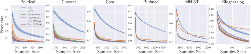
Figure 4: Error rate as the function of samples seen on six small-scale graphs.

Practical implementation. 

A caveat of approximate inversion in FastONL is that $\bm{M}_{\epsilon}$ is not in general symmetric; therefore, for analysis, we require $\bm{\psi}_{t}$ to be computed using the symmetrized $\bm{M}_{\epsilon}[:,t]+\bm{M}_{\epsilon}[t,:]$, which requires row and column access at time $t$; effectively, this requires that $\bm{M}_{\epsilon}$ is fully pre-computed. While this does not affect our overall bounds, the memory requirements may be burdensome. However, when $\bm{M}_{\epsilon}\approx\bm{M}$ (which is symmetric), then $(\bm{M}_{\epsilon})_{:,t}\approx(\bm{M}_{\epsilon})_{t,:}$ and in practice, we use the column to represent the row; our experiments show that this does not incur noticeable performance drop. To avoid pre-computing diagonal elements of $\bm{M}_{\epsilon}$, we estimate $\sum_{t=1}^{n}m_{tt}\approx kn^{2}$; experiments show this works well in practice.

Dynamic setting. 

An extension of our current setting is the dynamic setting, in which newly labeled nodes and their edges are dynamically added or deleted. As is, FastONL is well-suited to this extension; the key idea is to use an efficient method to keep updating FIFOPush, which can quickly keep track of these kernel vectors (Zhang et al., 2016, e.g.). The regret analysis of the dynamic setting is more challenging, and we will consider it as future work.

6 Experiments

In this section, we conduct extensive experiments on the online node classification for different-sized graphs and compare FastONL with baselines. We address the following questions: 1) Do these parameterized kernels work and capture label smoothness?; 2) How does FastONL compare in terms of classification accuracy and run time with baselines?

Experimental setup.  We collect ten graph datasets where nodes have true labels (Tab. 4) and create one large-scale Wikipedia graph where chronologically-order node labels are from ten categories of English Wikipedia articles. We consider four baselines, including 1) Weighted Majority (WM), where we predict each node $u$ by its previously labeled neighbors (a purely local but strong baseline described in Appendix D); 2) Relaxation (Rakhlin & Sridharan, 2017), a globally guaranteed method; 3) Weighted Tree Algorithm (WTA) (Cesa-Bianchi et al., 2013), a representative method based on sampling random spanning trees; and 4) Approximate, the power iteration-based method defined by Equ. (7). We implemented these baselines using Python. For FastONL, we chose the first two kernels defined in Tab. 1 and named them as FastONL-$\bm{K}_{1}$ and FastONL-$\bm{K}_{2}$, respectively. All experimental setups, including parameter tuning, are further discussed in Appendix D.

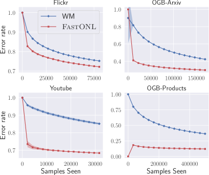
Figure 5: The comparison of error rate of FastONL and WM on middle-scale graphs.

Table 2: Run time of online node labeling methods over six graphs (seconds) averaged over 10 trials.

	Political	Citeseer	Cora	Pubmed	MNIST	Blogcatalog
WM	0.01	0.01	0.01	0.08	0.09	0.05
WTA	66.61	146.97	213.00	2177.49	10726.67	5108.45
Approximate	1.47	0.66	0.97	159.48	43.83	68.52
Relaxation	0.78	1.66	2.94	122.45	976.69	154.32
FastONL-$\bm{K}_{1}$	1.12	1.10	1.73	4.86	22.42	22.14
FastONL-$\bm{K}_{2}$	1.21	1.12	2.57	7.27	33.00	12.03

Online node labeling performance.  The online labeling error rates over 10 trials on small-scale graphs are presented in Fig. 4 where we pick $\epsilon=10^{-5}$. As we can see from Fig. 4, the approximated performance is almost the same as of Relaxation but with great improvements on runtime as shown in Tab. 2. The WM can be treated as a strong baseline. For middle and large-scale graphs, matrix inversion is infeasible, and these baselines are unavailable. We compare FastONL with the local method WM. Fig. 5 and 7 present the error rate as a function of the number of seen nodes. FastONL outperforms the local WM by a large margin. This indicates that FastONL has a better tradeoff between local and global consistency. The average run time of these methods is presented in Tab. 2. The local method WM has the lowest run time per iteration. Our method is between Relaxation and WTA.

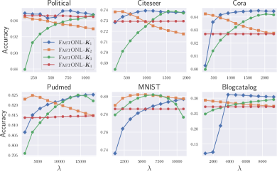
Figure 6: The accuracy of applying the first four kernel matrices for FastONL on six small graphs.

Performance of parameterized kernels.  In our theory, we showed what the effect of parameters $(\lambda,\beta)$ is on the regret (see Thm.5.1). The parameter $\lambda$ is a label smoothing parameter controlling the range of allowed label configurations while $\beta$ is the kernel parameter. We tested the first four kernels where kernels $\bm{K}_{1}$ and $\bm{K}_{2}$ solely depend on $\lambda$, while kernels $\bm{K}_{3}$ and $\bm{K}_{4}$ involve both $\lambda$ and $\beta$. However, for $\bm{K}_{3},\beta$ is defined as $\lambda/n$, and for $\bm{K}_{4}$, it is defined as $\beta=1-\lambda/n$, as established in Thm.5.1. By defining $\beta$ this way, our theorem ensures an effective regret. We experimented with various values of $\lambda$, selecting from $0.1\cdot n,0.2\cdot n,\ldots,0.9\cdot n,n$. Fig. 6 shows how different kernels perform over different graphs. All of the kernels successfully captured label smoothing but exhibited differing performances with varying $\lambda$. We consider the first four kernels as listed in Tab. 1, sweeping $\lambda$. To answer our first question, we find that all kernels can capture the label smoothing well but perform differently with different $\lambda$. Overall, the normalized kernel of $\bm{K}_{2}$ enjoys a large range of $\lambda$, while $\bm{K}_{1}$ and $\bm{K}_{3}$ tend to prefer big $\lambda$.

Case study of labeling Wikipedia articles.  We apply our method to a real-world Wikipedia graph, which contains 6,216,199 nodes where corresponding labels appear chronically and unweighted 177,862,656 edges (edges are hyperlinks among these Wikipedia articles). Each node may have a label (downloaded from DBpedia (2021), about 50% percentage of nodes have labels, we use the first 150,000 labeled nodes) belonging to ten categories describing the Wikipedia articles, such as people, places, etc. Fig. 7 presents our results on this large-scale graph. Compared with the strong baseline WM, our FastONL truly outperforms it by a large margin with only about 0.3 seconds for each article.

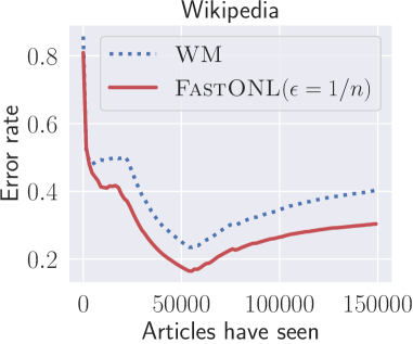
Figure 7: The comparison of error rate of FastONL and WM on one large-scale graph.

7 Conclusion

We study the online relaxation framework for the node labeling problem. We propose, for the first time, a fast approximate method that yields effective online regret bounds, filling a significant gap in the theoretical analysis of this online learning problem. We then design a general FIFOPush algorithm to quickly compute an approximate column of the kernel matrix in an online fashion that does not require large local memory storage. Therefore, the actual computational complexity per-iteration is truly local and competitive to other baseline methods. The local analysis of FIFOPush is challenging when the acceleration is added to the algorithm. It is interesting to see if there is any local analysis for accelerated algorithms (See the open question (Fountoulakis & Yang, 2022)). It is also interesting to see whether our work can be extended to directed or dynamic graph settings.

The appendix is organized as follows: Section A presents all missing proofs for graph kernel matrices computation and approximation. Section B proves the bounds of eigenvalues of $\bm{M}_{\epsilon}$ and $\bm{R}_{\epsilon}$. Section C provides the regret analysis. Section D presents more experimental details and results.

Appendix A Proofs

A.1 Graph kernel matrices and their equivalence: The proof of Thm. 4

Recall that our goal is to compute the following augmented kernel matrix

$$\bm{M}_{\lambda,\beta}=\left(\frac{{\bm{K}}_{\beta}^{-1}}{2\lambda}+\frac{\bm{I}_{n}}{2n}\right)^{-1}$$

for various instances of $\bm{K}_{\beta}^{-1}$ as listed in Table 1. The unnormalized Laplacian is defined as $\mathcal{\bm{L}}\triangleq\bm{D}-\bm{W}$ where $\bm{W}$ is the nonnegative symmetric weighted adjacency matrix, and $\bm{D}$ is the corresponding weighted degree matrix defined as $\mathbf{diag}{(\bm{W}\bm{1})}$. The normalized graph Laplacian is $\bm{L}\triangleq{\bm{D}}^{-1/2}\mathcal{\bm{L}}{\bm{D}}^{-1/2}$. Using FIFOPush, we can approximate the following two basic matrices

$$\text{Type-}\bm{L}:\quad\bm{X}_{\bm{L}}=\alpha\left(\bm{I}_{n}-(1-\alpha)\bm{W}\bm{D}^{-1}\right)^{-1},\quad\quad\quad\text{Type-}\mathcal{L}:\quad\bm{X}_{\mathcal{L}}=\left(\alpha\bm{I}_{n}+\bm{D}-\bm{W}\right)^{-1}.$$ (11)

We repeat our theorem in the following

Theorem 4.

Let $\bm{K}_{\beta}^{-1}$ be the inverse of the symmetric positive definite kernel matrix defined in Table 1. Then $\bm{M}_{\lambda,\beta}$ can be decomposed into $\bm{M}_{\lambda,\beta}=a\bm{A}^{-1}\bm{X}\bm{B}$, which is easily computed once $\bm{X}$ available. $\bm{X}$ represents two basic kernel inverse

$$\bm{X}_{\mathcal{L}}=\left(\alpha\bm{I}+\mathcal{L}\right)^{-1},\quad\bm{X}_{\bm{L}}=\alpha\left(\bm{I}-(1-\alpha)\bm{W}\bm{D}^{-1}\right)^{-1}$$

corresponding to inverse of regularized $\bm{L}$ and $\mathcal{L}$, respectively.

Proof.

We now show how each of these kernels $\bm{K}$ can be efficiently computed given either $\bm{X}_{\bm{L}}$ or $\bm{X}_{\mathcal{L}}$ as follows:

Instance 1. 

For the kernel $\bm{K}_{\beta}^{-1}=\mathcal{\bm{L}}$, we have

$$\left(\frac{\bm{K}_{\beta}^{-1}}{2\lambda}+\frac{\bm{I}_{n}}{2n}\right)^{-1} =\left(\frac{\mathcal{\bm{L}}}{2\lambda}+\frac{\bm{I}_{n}}{2n}\right)^{-1}$$

$$=\left(\frac{\bm{D}-\bm{W}}{2\lambda}+\frac{\bm{I}_{n}}{2n}\right)^{-1}$$

$$=2\lambda\left(\alpha\bm{I}_{n}+\bm{D}-\bm{W}\right)^{-1}$$

$$=2\lambda\bm{X}_{\mathcal{\bm{L}}},$$

where we let $\alpha=\tfrac{\lambda}{n}$.

Instance 2. 

For the kernel $\bm{K}_{\beta}^{-1}=\bm{I}-\bm{D}^{-1/2}\bm{W}{\bm{D}}^{-1/2}$, we have

$$\left(\frac{\bm{K}_{\beta}^{-1}}{2\lambda}+\frac{\bm{I}_{n}}{2n}\right)^{-1} =\left(\frac{\bm{I}_{n}-{\bm{D}}^{-1/2}{\bm{W}}{\bm{D}}^{-1/2}}{2\lambda}+\frac{\bm{I}_{n}}{2n}\right)^{-1}$$

$$=\left(\frac{1}{2\lambda}+\frac{1}{2n}\right)^{-1}\cdot\left(\bm{I}_{n}-\frac{\left(\frac{1}{2\lambda}+\frac{1}{2n}\right)^{-1}}{2\lambda}{\bm{D}}^{-1/2}{\bm{W}}{\bm{D}}^{-1/2}\right)^{-1}$$

$$=\frac{2n\lambda}{n+\lambda}{\bm{D}}^{-1/2}\left(\bm{I}_{n}-\frac{n}{n+\lambda}\bm{W}{\bm{D}}^{-1}\right)^{-1}{\bm{D}}^{1/2}$$

$$=2n\alpha{\bm{D}}^{-1/2}\left(\bm{I}_{n}-(1-\alpha)\bm{W}{\bm{D}}^{-1}\right)^{-1}{\bm{D}}^{1/2}$$

$$=2n{\bm{D}}^{-1/2}\bm{X}_{\bm{L}}{\bm{D}}^{1/2},$$

where $\alpha=\frac{\lambda}{n+\lambda}$.

Instance 3. 

The kernel $\bm{K}_{\beta}^{-1}=\bm{I}-\beta\bm{D}^{-1/2}\bm{W}{\bm{D}}^{-1/2}$. Different from Instance 2, the kernel is now parameterized. Specifically, we have

$$\left(\frac{\bm{K}_{\beta}^{-1}}{2\lambda}+\frac{\bm{I}_{n}}{2n}\right)^{-1} =\left(\frac{\bm{I}_{n}-\beta{\bm{D}}^{-1/2}{\bm{W}}{\bm{D}}^{-1/2}}{2\lambda}+\frac{\bm{I}_{n}}{2n}\right)^{-1}$$

$$=\left(\frac{1}{2\lambda}+\frac{1}{2n}\right)^{-1}\cdot\left(\bm{I}_{n}-\frac{\beta\left(\frac{1}{2\lambda}+\frac{1}{2n}\right)^{-1}}{2\lambda}{\bm{D}}^{-1/2}{\bm{W}}{\bm{D}}^{-1/2}\right)^{-1}$$

$$=\frac{2n\lambda}{n+\lambda}{\bm{D}}^{-1/2}\left(\bm{I}_{n}-\frac{\beta n}{n+\lambda}\bm{W}{\bm{D}}^{-1}\right)^{-1}{\bm{D}}^{1/2}$$

$$=\frac{2n\lambda}{(n+\lambda)\alpha}{\bm{D}}^{-1/2}\alpha\left(\bm{I}_{n}-(1-\alpha)\bm{W}{\bm{D}}^{-1}\right)^{-1}{\bm{D}}^{1/2}=\frac{2\lambda n}{n+\lambda-n\beta}{\bm{D}}^{-1/2}\bm{X}_{\bm{L}}{\bm{D}}^{1/2},$$

where $1-\alpha=\frac{n\beta}{n+\lambda}$, and the parameter $\beta\in(0,\frac{n+\lambda}{n})$.

Instance 4. 

The kernel $\bm{K}_{\beta}^{-1}=\beta{\bm{I}}+{\bm{S}}^{-1/2}\mathcal{\bm{L}}{\bm{S}}^{-1/2}$ was initially considered in Johnson & Zhang (2008) where $\bm{S}$ is a positive diagonal matrix. Typical examples of $\bm{S}$ could be $\bm{D}$, $\bm{I}$, etc. Note that

$$\left(\frac{\bm{K}_{\beta}^{-1}}{2\lambda}+\frac{\bm{I}_{n}}{2n}\right)^{-1} =\left(\frac{\beta{\bm{I}}+{\bm{S}}^{-1/2}{\mathcal{L}}{\bm{S}}^{-1/2}}{2\lambda}+\frac{\bm{I}_{n}}{2n}\right)^{-1}$$

$$=\left(\frac{1}{b}\left(ab{\bm{I}}+{\bm{S}}^{-1/2}(\bm{D}-\bm{W}){\bm{S}}^{-1/2}\right)\right)^{-1}\text{\quad\quad// let $a=\left(\frac{\beta}{2\lambda}+\frac{1}{2n}\right),b=2\lambda$}$$

$$=b{\bm{S}}^{1/2}\left(ab{\bm{S}}+\bm{D}-\bm{W}\right)^{-1}{\bm{S}}^{1/2}$$

$$=b{\bm{S}}^{-1/2}\left(ab{\bm{I}}+\left(\bm{D}-\bm{W}\right)\bm{S}^{-1}\right)^{-1}{\bm{S}}^{1/2}$$

$$=b{\bm{S}}^{-1/2}\left(ab{\bm{I}}+\left(\bm{D}-\bm{W}\right)\bm{S}^{-1}\right)^{-1}{\bm{S}}^{1/2}$$

$$=2\lambda{\bm{S}}^{-1/2}\bm{X}_{\mathcal{L}}{\bm{S}}^{1/2},$$

where $\alpha=\frac{\beta n+\lambda}{n}$. Note $\left(\bm{D}-\bm{W}\right)\bm{S}^{-1}$ is a positive semidefinite matrix as $\bm{D}-\bm{W}$ is positive semidefinite and $\bm{S}^{-1}$ is positive definite, then applying $\bm{D}^{{}^{\prime}}=\bm{D}\bm{S}^{-1}$ and $\bm{W}^{{}^{\prime}}=\bm{W}\bm{S}^{-1}$. Therefore, it is essential to solve $(\alpha\bm{I}+\bm{D}^{\prime}-\bm{W}^{\prime})^{-1}$ because $\bm{D}^{\prime}-\bm{W}^{\prime}$ has nonnegative eigenvalues and $D^{\prime}_{u}=\sum_{v\in\mathcal{N}{(u)}}W^{\prime}_{uv}$ for all $u\in\mathcal{V}$. Therefore, it belongs to Type-II. Here, we abuse notations where we let $\bm{D}=\bm{D}^{\prime}$ and $\bm{W}=\bm{W}^{\prime}$.

Instance 5. 

The normalized kernel matrix $\bm{K}_{\beta}^{-1}={\bm{S}}^{-1/2}{\left(\beta{\bm{I}}+\mathcal{L}\right)}{\bm{S}}^{-1/2}$, the $\bm{S}$ is the normalization matrix (Ando & Zhang, 2006; Johnson & Zhang, 2007). Just like Instance 4, we could have different choices for $\bm{S}$: $\bm{I}$, $\bm{D}$, or $(\beta\bm{I}+\mathcal{L})^{-1}$ (for the last case, the kernel is then normalized with unit diagonal), etc. Note

$$\left(\frac{\bm{K}_{\beta}^{-1}}{2\lambda}+\frac{\bm{I}_{n}}{2n}\right)^{-1} =\left(\frac{{\bm{S}}^{-1/2}(\beta{\bm{I}}+\mathcal{L}){\bm{S}}^{-1/2}}{2\lambda}+\frac{\bm{I}_{n}}{2n}\right)^{-1}$$

$$={\bm{S}}^{1/2}\left(\tilde{\bm{S}}+\frac{\mathcal{L}}{2\lambda}\right)^{-1}{\bm{S}}^{1/2}\text{\quad\quad\quad// let $\tilde{\bm{S}}=\frac{\beta\bm{I}}{2\lambda}+\frac{\bm{S}}{2n}$}$$

$$=2\lambda{\bm{S}}^{1/2}\left(2\lambda\tilde{\bm{S}}+\mathcal{L}\right)^{-1}{\bm{S}}^{1/2}$$

$$=2\lambda{\bm{S}}^{1/2}\tilde{\bm{S}}^{-1}\left(2\lambda\bm{I}+(\bm{D}-\bm{W})\tilde{\bm{S}}^{-1}\right)^{-1}{\bm{S}}^{1/2},$$

where $(\bm{D}-\bm{W})\tilde{\bm{S}}^{-1}$ is a transformed version of $\mathcal{L}$. We continue to have

$$\left(\frac{\bm{K}_{\beta}^{-1}}{2\lambda}+\frac{\bm{I}_{n}}{2n}\right)^{-1} =2\lambda{\bm{S}}^{1/2}\tilde{\bm{S}}^{-1}\left(2\lambda\bm{I}+(\bm{D}-\bm{W})\tilde{\bm{S}}^{-1}\right)^{-1}{\bm{S}}^{1/2}$$

$$=2\lambda{\bm{S}}^{1/2}{\left(\frac{\beta\bm{I}}{2\lambda}+\frac{\bm{S}}{2n}\right)}^{-1}\left(2\lambda\bm{I}+(\bm{D}-\bm{W})\tilde{\bm{S}}^{-1}\right)^{-1}{\bm{S}}^{1/2}$$

$$=\left(\frac{\bm{S}^{1/2}}{4n\lambda}+\frac{\beta\bm{S}^{-1/2}}{4\lambda^{2}}\right)^{-1}\bm{X}_{\mathcal{L}}{\bm{S}}^{1/2},$$

where $\alpha=2\lambda$. Similar to Instance 4, $(\bm{D}-\bm{W})\tilde{\bm{S}}^{-1}$ is transformed Laplacian matrix. Let $\bm{D}^{\prime}=\bm{D}\tilde{\bm{S}}^{-1}$ and $\bm{W}^{\prime}=\bm{W}\tilde{\bm{S}}^{-1}$. We abuse of notations of $\bm{D},\bm{W}$ and let $\bm{D}=\bm{D}^{\prime}$ and $\bm{W}=\bm{W}^{\prime}$.

Instance 6.  The augmented kernel $\bm{K}_{\lambda}=\mathcal{\bm{L}}+b\cdot\bm{1}\bm{1}^{\top}+\beta\bm{I}$ (Herbster et al., 2005) can be reformulated as

$$\left(\frac{\bm{K}_{\beta}^{-1}}{2\lambda}+\frac{\bm{I}_{n}}{2n}\right)^{-1} =\left(\frac{\mathcal{\bm{L}}+b\cdot\bm{1}\bm{1}^{\top}+\beta\bm{I}}{2\lambda}+\frac{\bm{I}}{2n}\right)^{-1}$$

$$=\left(\frac{\mathcal{\bm{L}}+\beta\bm{I}}{2\lambda}+\frac{\bm{I}}{2n}+\frac{b\cdot\bm{1}\bm{1}^{\top}}{2\lambda}\right)^{-1}$$

$$=2\lambda\bm{X}_{\mathcal{L}}\left(\bm{I}-\frac{b\bm{1}\bm{1}^{\top}\bm{X}_{\mathcal{L}}}{1+b\bm{1}^{\top}\bm{X}_{\mathcal{L}}\bm{1}}\right),$$

where $\alpha=\beta+\frac{\lambda}{n}$ and we use the similar method as in Instance 4 but plus a rank one matrix $\bm{1}\bm{1}^{\top}$. The last equality is from the fact that, for any invertible matrix $\bm{X}$, by the Sherman–Morrison formula, we have

$$(\bm{X}+\bm{1}\bm{1}^{\top})^{-1}=\bm{X}^{-1}-\frac{\bm{X}^{-1}\bm{1}\bm{1}^{\top}\bm{X}^{-1}}{1+\bm{1}^{\top}\bm{X}^{-1}\bm{1}}.$$

Furthermore, note the summation of each column of $(\alpha\bm{I}+\mathcal{L})^{-1}$ is a constant $1/\alpha$, then $\bm{1}^{\top}\bm{X}_{\mathcal{L}}\bm{1}=n/\alpha$. Then, we continue to have

$$\left(\frac{\bm{K}_{\beta}^{-1}}{2\lambda}+\frac{\bm{I}_{n}}{2n}\right)^{-1} =2\lambda\bm{X}_{\mathcal{L}}\left(\bm{I}-\frac{b\bm{1}\bm{1}^{\top}\bm{X}_{\mathcal{L}}}{1+b\bm{1}^{\top}\bm{X}_{\mathcal{L}}\bm{1}}\right)$$

$$=2\lambda\bm{X}_{\mathcal{L}}\left(\bm{I}-\frac{\alpha b\bm{1}\bm{1}^{\top}\bm{X}_{\mathcal{L}}}{\alpha+nb}\right)$$

$$=2\lambda\bm{X}_{\mathcal{L}}\left(\bm{I}-\frac{b\bm{1}\bm{1}^{\top}}{\alpha+nb}\right),$$

where note that $\bm{1}\bm{1}^{\top}\bm{X}_{\mathcal{L}}=\bm{1}\bm{1}^{\top}/\alpha$. ∎

A.2 Local linear convergence of FIFOPush for $\alpha\left(\bm{I}-(1-\alpha)\bm{W}\bm{D}^{-1}\right)^{-1}\bm{e}_{s}$: The proof of Thm. 4.2

Given any $\alpha\in(0,1),\epsilon>0$, Algorithm 4 is to approximate $\alpha\left(\bm{I}-(1-\alpha)\bm{W}\bm{D}^{-1}\right)^{-1}\bm{e}_{s}$. Before the proof of Theorem 4.2, we provide an equivalent version of FIFOPush as presented in Algorithm 4 where time index $t$ of $\bm{r},\bm{x}$ and time index $t^{\prime}$ of processed nodes $u$ are added. Our proof is based on this equivalent version. Compared with Algorithm 2, the only difference is that we added a dummy node ${\color[rgb]{1,0,0}{\ddagger}}$. Still, Algorithm 4 is essentially the same as Algorithm 2. The chronological order of processed nodes $u_{t^{\prime}}$ by FIFOPush can then be represented as the following order

Algorithm 4 $\textsc{FIFOPush}(\mathcal{G},\epsilon,\alpha,s)$(Andersen et al., 2006) with a dummy node ${\color[rgb]{1,0,0}{\ddagger}}$

1:  Initialize: $\bm{r}_{t}=\bm{e}_{s},\ \ \bm{x}_{t}=\bm{0},\ \ t=1,\ \ t^{\prime}=1$

2:  $\mathcal{Q}=[s,{\color[rgb]{1,0,0}{\ddagger}}]$          // At the initial stage, $\mathcal{Q}$ contains $s$ and a dummy node ${\color[rgb]{1,0,0}{\ddagger}}$.

3:  while $\mathcal{Q}\text{.size}()\neq 1$ do

4:     $u_{t^{\prime}}=\mathcal{Q}\text{.pop()}$

5:     if $u_{t^{\prime}}=={\color[rgb]{1,0,0}{\ddagger}}$ then

6:        $t=t+1$       // Nodes in $\mathcal{U}_{t}$ has been processed. Go to the next epoch.

7:        $\mathcal{Q}\text{.push}(u_{t^{\prime}})$

8:        continue

9:     end if

10:     if $r_{u_{t^{\prime}}}<\epsilon\cdot d_{u_{t^{\prime}}}$ then

11:        $t^{\prime}=t^{\prime}+1$        // $u_{t^{\prime}}$ is an “inactive” node

12:        continue

13:     end if

14:     $x_{u_{t^{\prime}}}=x_{u_{t^{\prime}}}+\alpha r_{u_{t^{\prime}}}$    // $u_{t^{\prime}}$ is an “active” node

15:     for $v\in\mathcal{N}(u_{t^{\prime}})$ do

16:        $r_{v}=r_{v}+\frac{(1-\alpha)r_{u_{t^{\prime}}}}{D_{u_{t^{\prime}}}}\cdot w_{u_{t^{\prime}}v}$

17:        if $v\notin\mathcal{Q}$ then

18:           $\mathcal{Q}\text{.push}(v)$

19:        end if

20:     end for

21:     $r_{u_{t^{\prime}}}=0$

22:     $t^{\prime}=t^{\prime}+1$

23:  end while

24:  Return $(\bm{x}_{t},\bm{r}_{t})$

$$\ {\color[rgb]{1,0,0}{\ddagger}}\ \underbrace{u_{1}}_{\mathcal{U}_{1}}\ {\color[rgb]{1,0,0}{\ddagger}}\ \underbrace{u_{2},u_{3},\ldots}_{\mathcal{U}_{2}}\ {\color[rgb]{1,0,0}{\ddagger}}\ \cdots\ {\color[rgb]{1,0,0}{\ddagger}}\ \underbrace{u_{t^{\prime}},u_{t^{\prime}+1},u_{t^{\prime}+2},\ldots,u_{t^{\prime}+i}}_{\mathcal{U}_{t}}\ {\color[rgb]{1,0,0}{\ddagger}}\ \cdots,$$ (12)

where $\mathcal{U}_{t}=\{u_{t^{\prime}},u_{t^{\prime}+1},\ldots,u_{t^{\prime}+i}\}$ is the set of nodes processed in $t$-th epoch. Hence, (12) defines super epochs indexed by $t$ where $\mathcal{U}_{t}$ will be processed. From epoch $t$, new nodes will be added into $\mathcal{Q}$ for the next epoch as illustrated in Fig. 1. $\mathcal{U}_{t}$ contains: 1) a set of active nodes $\mathcal{S}_{t}\triangleq\left\{u_{t^{\prime}}:r_{u_{t^{\prime}}}\geq\epsilon\cdot d_{u_{t^{\prime}}},u_{t^{\prime}}\in\mathcal{U}_{t}\right\}$; and 2) a set of inactive nodes $\left\{u_{t^{\prime}}:0<r_{u_{t^{\prime}}}<\epsilon\cdot d_{u_{t^{\prime}}},u_{t^{\prime}}\in\mathcal{U}_{t}\right\}=\mathcal{U}_{t}\backslash\mathcal{S}_{t}$. FIFOPush terminates only when $\mathcal{Q}$ contains the dummy node ${\color[rgb]{1,0,0}{\ddagger}}$.

Define $\bm{X}=\alpha\left(\bm{I}-(1-\alpha)\bm{W}\bm{D}^{-1}\right)^{-1}$. Denote the estimation matrix $\bm{X}_{\epsilon}=\left[\bm{x}_{1,\epsilon},\ldots,\bm{x}_{n,\epsilon}\right]$ and the residual matrix $\bm{R}_{\epsilon}=\left[\bm{r}_{1,\epsilon},\ldots,\bm{r}_{n,\epsilon}\right]$ where $(\bm{x}_{s,\epsilon},\bm{r}_{s,\epsilon})=\textsc{FIFOPush}(\mathcal{G},\epsilon,\alpha,s)$ for all $s\in\mathcal{V}$. The next lemma shows that $\bm{X}_{\epsilon}$ is a good approximation of $\bm{X}$ from the bottom when $\epsilon$ is small.

Lemma A.1.

Let $\bm{X}=\alpha\left(\bm{I}-(1-\alpha)\bm{W}\bm{D}^{-1}\right)^{-1}$ and denote $s$-th column of $\bm{X}$ as $\bm{x}_{s}=\alpha\left(\bm{I}-(1-\alpha)\bm{W}\bm{D}^{-1}\right)^{-1}{\bm{e}}_{s}$. Let $({\bm{x}}_{s,\epsilon},\bm{r}_{s,\epsilon})=\textsc{FIFOPush}(\mathcal{G},\epsilon,\alpha,s)$ be the pair of vectors returned by Alg. 4 where $\bm{x}_{s,\epsilon}$ is an estimate of $\bm{x}_{s}$ and $\bm{r}_{s,\epsilon}$ is the corresponding residual vector. Denote the estimation matrix $\bm{X}_{\epsilon}=\left[\bm{x}_{1,\epsilon},\ldots,\bm{x}_{n,\epsilon}\right]$ and the residual matrix $\bm{R}_{\epsilon}=\left[\bm{r}_{1,\epsilon},\ldots,\bm{r}_{n,\epsilon}\right]$ by calling FIFOPush for all $s\in\mathcal{V}$. For any $\epsilon>0$, we have

$$\bm{X}=\bm{X}_{\epsilon}+\bm{X}\bm{R}_{\epsilon},$$

where $\bm{R}_{\epsilon}$ satisfies $\bm{0}_{n\times n}\leq\bm{R}_{\epsilon}<\epsilon\cdot\mathbf{diag}{(d_{1},\ldots,d_{n})}\cdot\bm{1}\bm{1}^{\top}$.

Proof.

Let us assume $t=t^{\prime}$ at the beginning of $t$-th epoch. During the $t$-th epoch, FIFOPush updates $t$ to $t+1$ and updates $t^{\prime}$ from $t^{\prime}=t_{0}^{\prime},t_{1}^{\prime},t_{2}^{\prime},\ldots$ to $t_{|\mathcal{S}_{t}|}^{\prime}=t+1$ where $t_{i}^{\prime}$ is the time after the update of node $u_{t_{i}^{\prime}}$. Recall $\mathcal{S}_{t}$ is the set of processed active nodes (at the beginning of $t$-th epoch, we do not know how many nodes in $\mathcal{S}_{t}$ since some inactive nodes could be active after some push operations). For each active node $u_{t_{i}^{\prime}}$ ($i=1,2,\ldots,|\mathcal{S}_{t}|$) at $t$-th epoch, we denote $\bm{x}_{u_{t_{i}^{\prime}}}$ and $\bm{r}_{u_{t_{i}^{\prime}}}$ as the updated vectors of $\bm{x}_{t}$ and $\bm{r}_{t}$, respectively. After all active nodes $u_{t_{i}^{\prime}}\in\mathcal{S}_{t}$ have been processed, $\bm{x}$ is updated from $\bm{x}_{t}$ to $\bm{x}_{t+1}$ and $\bm{r}$ from $\bm{r}_{t}$ to $\bm{r}_{t+1}$ as the following

$$\bm{x}_{t} =\bm{x}_{u_{t_{0}^{\prime}}}\xrightarrow[]{u_{t_{1}^{\prime}}}{\bm{x}}_{t_{1}^{\prime}}\xrightarrow[]{u_{t_{2}^{\prime}}}{\bm{x}}_{t_{2}^{\prime}}\quad\cdots\quad\xrightarrow[]{u_{t_{|\mathcal{S}_{t}|}^{\prime}}}{\bm{x}}_{t_{|\mathcal{S}_{t}|}^{\prime}}=\bm{x}_{t+1}$$

$$\bm{r}_{t} =\bm{r}_{u_{t_{0}^{\prime}}}\xrightarrow[]{u_{t_{1}^{\prime}}}{\bm{r}}_{u_{t_{1}^{\prime}}}\xrightarrow[]{u_{t_{2}^{\prime}}}{\bm{r}}_{u_{t_{2}^{\prime}}}\quad\cdots\quad\xrightarrow[]{u_{t_{|\mathcal{S}_{t}|}^{\prime}}}{\bm{r}}_{u_{{|\mathcal{S}_{t}|}}^{\prime}}=\bm{r}_{t+1}.$$

For each $i$-th active node $u_{t_{i}^{\prime}}$, the updates are from Line 14 to Line 21 of Alg. 4 give us the following iterations

$${\bm{x}}_{t_{i}^{\prime}} =\bm{x}_{t_{i-1}^{\prime}}\underbrace{+\alpha r_{u_{t_{i-1}^{\prime}}}\cdot\bm{e}_{u_{t_{i-1}^{\prime}}}}_{\text{Line 14}}$$ (13)

$${\bm{r}}_{t_{i}^{\prime}} =\bm{r}_{t_{i-1}^{\prime}}\underbrace{+(1-\alpha)r_{u_{t_{i-1}^{\prime}}}\cdot\bm{W}\bm{D}^{-1}\bm{e}_{u_{t_{i-1}^{\prime}}}}_{\text{Line 15,16}}\ \underbrace{-r_{u_{t_{i-1}^{\prime}}}\cdot\bm{e}_{u_{t_{i-1}^{\prime}}}}_{\text{Line 21}}.$$ (14)

These two iterations (13) and (14) essentially moves residual $r_{u_{t_{i-1}^{\prime}}}$ out of node $u_{t_{i-1}^{\prime}}$ to its estimate vector $\bm{x}$ and residual entries of its neighbors. Specifically, the first iteration (13) moves $\alpha$ times magnitude of $r_{u_{t_{i-1}^{\prime}}}$ to $\bm{x}$ and the second iteration (14) moves $(1-\alpha)$ times of $r_{u_{t_{i-1}^{\prime}}}$ to neighbors spread the magnitude by the distribution vector $\bm{W}\bm{D}^{-1}\bm{e}_{u_{t_{i-1}^{\prime}}}$. The last term $-r_{u_{t_{i-1}^{\prime}}}\cdot\bm{e}_{u_{t_{i-1}^{\prime}}}$ is to remove $r_{u_{t_{i-1}^{\prime}}}$ from node $u_{t_{i-1}^{\prime}}$. Rearrange (14), we have

$${\bm{r}}_{t_{i}^{\prime}} =\bm{r}_{t_{i-1}^{\prime}}+(1-\alpha)r_{u_{t_{i-1}^{\prime}}}\cdot\bm{W}\bm{D}^{-1}\bm{e}_{u_{t_{i-1}^{\prime}}}-r_{u_{t_{i-1}^{\prime}}}\cdot\bm{e}_{u_{t_{i-1}^{\prime}}}$$

$${\bm{r}}_{t_{i}^{\prime}} =\bm{r}_{t_{i-1}^{\prime}}-\left(\bm{I}-(1-\alpha)\bm{W}\bm{D}^{-1}\right)r_{u_{t_{i-1}^{\prime}}}\cdot\bm{e}_{u_{t_{i-1}^{\prime}}}$$

$$\alpha r_{u_{t_{i-1}^{\prime}}}\cdot\bm{e}_{u_{t_{i-1}^{\prime}}} =\alpha\left(\bm{I}-(1-\alpha)\bm{W}\bm{D}^{-1}\right)^{-1}\left(\bm{r}_{t_{i-1}^{\prime}}-{\bm{r}}_{t_{i}^{\prime}}\right).$$ (15)

Use (15) and (13), we have

$${\bm{x}}_{t_{i}^{\prime}} =\bm{x}_{t_{i-1}^{\prime}}+\alpha r_{u_{t_{i-1}^{\prime}}}\cdot\bm{e}_{u_{t_{i-1}^{\prime}}}$$

$$=\bm{x}_{t_{i-1}^{\prime}}+\alpha\left(\bm{I}-(1-\alpha)\bm{W}\bm{D}^{-1}\right)^{-1}\left(\bm{r}_{t_{i-1}^{\prime}}-{\bm{r}}_{t_{i}^{\prime}}\right)$$

Since $i=1,2,\ldots,|\mathcal{S}_{t}|$, we sum above equation over all active nodes $\mathcal{S}_{t}$, we have

$${\bm{x}}_{t+1} ={\bm{x}}_{t_{|\mathcal{S}_{t}|^{\prime}}}$$

$$=\bm{x}_{t_{{|\mathcal{S}_{t}|-1}^{\prime}}}+\alpha\left(\bm{I}-(1-\alpha)\bm{W}\bm{D}^{-1}\right)^{-1}\left(\bm{r}_{t_{|\mathcal{S}_{t}|-1}^{\prime}}-{\bm{r}}_{t_{|\mathcal{S}_{t}|}^{\prime}}\right)$$

$$\vdots$$

$$=\bm{x}_{t_{0^{\prime}}}+\alpha\left(\bm{I}-(1-\alpha)\bm{W}\bm{D}^{-1}\right)^{-1}\sum_{i=1}^{|\mathcal{S}_{t}|}\left(\bm{r}_{t_{i-1}^{\prime}}-{\bm{r}}_{t_{i}^{\prime}}\right)$$

$$=\bm{x}_{t_{0^{\prime}}}+\alpha\left(\bm{I}-(1-\alpha)\bm{W}\bm{D}^{-1}\right)^{-1}\left(\bm{r}_{t_{0}^{\prime}}-{\bm{r}}_{t_{|\mathcal{S}_{t}|}^{\prime}}\right)$$

$$=\bm{x}_{t}+\alpha\left(\bm{I}-(1-\alpha)\bm{W}\bm{D}^{-1}\right)^{-1}\left(\bm{r}_{t}-{\bm{r}}_{t+1}\right)$$

On the other hand, for all epochs, we continue to use the last equation to have

$$\bm{x}_{t+1} =\bm{x}_{t}+\alpha\left(\bm{I}-(1-\alpha)\bm{W}\bm{D}^{-1}\right)^{-1}\left(\bm{r}_{t}-\bm{r}_{t+1}\right)$$

$$=\alpha\left(\bm{I}-(1-\alpha)\bm{W}\bm{D}^{-1}\right)^{-1}\sum_{i=1}^{t}\left(\bm{r}_{i}-\bm{r}_{i+1}\right)$$

$$=\alpha\left(\bm{I}-(1-\alpha)\bm{W}\bm{D}^{-1}\right)^{-1}\left(\bm{r}_{1}-\bm{r}_{t+1}\right)$$

$$=\bm{X}(\bm{e}_{s}-\bm{r}_{t+1}).$$ (16)

Since $\bm{x}_{s,\epsilon}$ is an estimate of $\bm{x}_{s}$ returned by FIFOPush, for any node $s\in\mathcal{V}$ and by (16), we have

$$\bm{X}\bm{e}_{s}={\bm{x}}_{s,\epsilon}+\bm{X}\bm{r}_{s,\epsilon},\quad\forall s\in\mathcal{V}.$$

Write the above equation as a matrix form; we obtain $\bm{X}=\bm{X}_{\epsilon}+\bm{X}\bm{R}_{\epsilon}$. Notice that each $u$-th element of $\bm{r}_{s,\epsilon}$ satisfies $0\leq r_{s,\epsilon}(u)<\epsilon d_{u}$. Hence we have ${\bm{0}}_{n\times n}\leq\bm{R}_{\epsilon}<\epsilon\cdot\mathbf{diag}{(d_{1},\ldots,d_{n})}\cdot\bm{1}\bm{1}^{\top}$. ∎

Remark A.2.

The above lemma is essentially the linear invariant property (Andersen et al., 2006). Here, we show a relation between the estimation and residual vectors. Recall that for any subset of nodes $\mathcal{S}\subseteq\mathcal{V}$, the volume of $\mathcal{S}$ is defined $\operatorname{vol}\left(\mathcal{S}\right)=\sum_{v\in\mathcal{S}}d_{v}$. We are ready to prove Thm. 4.2.

Theorem 4.2 (Local linear convergence of FIFOPush for $\bm{X}_{\bm{L}}$).

Let $\bm{x}_{s}=\bm{X}_{\bm{L}}\bm{e}_{s}$. Denote $T$ as the total epochs executed by FIFOPush, and $\mathcal{S}_{t}:=\{v:r_{t}(v)\geq\epsilon\cdot d_{v},v\in\mathcal{I}_{t}\}$ as the set of active nodes in $t$-th epoch. Then, the total operations of $\textsc{FIFOPush}(\mathcal{G},\epsilon,\alpha,s)$ is dominated by

$$R_{T}:=\sum_{t=1}^{T}\sum_{u_{t}\in{\mathcal{S}}_{t}}d_{u_{t}}\leq\frac{\operatorname{vol}\left(\mathcal{S}_{1:T}\right)}{\alpha\cdot\eta_{1:T}}\log\left(\frac{C_{\alpha,T}}{\epsilon}\right),$$ (17)

where $\operatorname{vol}\left(\mathcal{S}_{1:T}\right)=\sum_{t=1}^{T}\operatorname{vol}\left(\mathcal{S}_{t}\right)/T$ is the average volume of $\mathcal{S}_{t}$. Additionally, $\eta_{1:T}=\sum_{t=1}^{T}\eta_{t}/T$ is the average of local convergence factors $\eta_{t}\triangleq\sum_{u\in\mathcal{S}_{t}}d_{u}/\sum_{v\in\mathcal{I}_{t}}d_{v}$, and $C_{\alpha,T}=1/(\sum_{v\in\mathcal{I}_{T}}(1-\alpha)d_{u}w_{uv}/D_{u})$. For $s,i\in\mathcal{V}$, we have $\bm{x}_{s}=\bm{x}_{s,\epsilon}+\bm{X}_{\bm{L}}\bm{r}_{s,\epsilon},r_{s,\epsilon}(i)\leq[0,\epsilon d_{i})$.

Proof of Theorem 4.2.

From Lemma A.1, we know that for $s,i\in\mathcal{V}$, we have $\bm{x}_{s}=\bm{x}_{s,\epsilon}+\bm{X}_{\bm{L}}\bm{r}_{s,\epsilon},r_{s,\epsilon}(i)\leq[0,\epsilon d_{i})$. At epoch $t\geq 1$, recall $\mathcal{Q}$ contains a set of active nodes $\mathcal{S}_{t}$ and a set of inactive nodes $\mathcal{U}_{t}\backslash\mathcal{S}_{t}$. After FIFOPush processed the last node $u_{t^{\prime}+i}$ in $\mathcal{U}_{t}$, it is easy to see that the total operations of $t$-th epoch are dominated by the volume of $\mathcal{S}_{t}$, i.e., $\operatorname{vol}\left(\mathcal{S}_{t}\right)$ (from Line 13 to Line 16). Hence, the total time complexity is dominated by $R_{T}=\sum_{t=1}^{T}\operatorname{vol}\left(\mathcal{S}_{t}\right)$. In the rest, we shall provide two upper bounds of $R_{T}$.

1. The first is to prove an upper bound $1/\alpha\epsilon$, which is directly followed from Andersen et al. (2006). We repeat the main idea here. For each active iteration of Algo. 4, we have $r_{u_{t^{\prime}}}\geq\epsilon\cdot d_{u_{t^{\prime}}}$, which indicates $r_{u_{t^{\prime}}}$ was at least $\epsilon\cdot d_{u_{t^{\prime}}}$; hence $\|\bm{r}_{t}\|_{1}$ decreased by at least $\alpha\epsilon\cdot d_{u_{t^{\prime}}}$ with total $d_{u_{t^{\prime}}}$ operations. Hence, overall $u_{t^{\prime}}\in\mathcal{S}_{t}$, we have

   $$\alpha\epsilon\sum_{u_{t^{\prime}}\in\mathcal{S}_{t}}d_{u_{t^{\prime}}}\leq\alpha\sum_{u_{t^{\prime}}\in\mathcal{S}_{t}}r_{u_{t^{\prime}}}=\|\bm{r}_{t}\|_{1}-\|\bm{r}_{t+1}\|_{1}.$$

   Summing the above inequality over $t$, we have the total operations of FIFOPush bounded by

   $$R_{T}=\sum_{t=1}^{T}\operatorname{vol}\left(\mathcal{S}_{t}\right)=\sum_{t=1}^{T}\sum_{u\in\mathcal{S}_{t}}d_{u}\leq\frac{1}{\alpha\epsilon}\sum_{t=1}^{T}\left(\|\bm{r}_{t}\|_{1}-\|\bm{r}_{t+1}\|_{1}\right)=\frac{1-\|\bm{r}_{T+1}\|_{1}}{\alpha\epsilon}\leq\frac{1}{\alpha\epsilon},$$ (18)

   where note that $\|\bm{r}_{1}\|_{1}=1$.

2. The sublinear bound $\mathcal{O}(\tfrac{1}{\alpha\epsilon})$ in (18) is independent of the graph size which is the key advantage of FIFOPush over other numerical methods such as Power Iteration where $\mathcal{O}(\tfrac{m}{\alpha}\log(\tfrac{1}{\epsilon}))$ operations needed, where $m$ is the number of edges in the graph. However, when $\epsilon$ becomes small, $\mathcal{O}(\tfrac{1}{\alpha\epsilon})$ is too pessimistic. It is natural to ask whether there exists any bound that takes advantage of both FIFOPush and PowerIter. We answer this question positively by providing a local linear convergence. There are two key components in our proof: 1) residuals left in $\bm{r}_{T}$ are relatively significant so that total epochs $T$ can be bound by $\mathcal{O}(\log\tfrac{1}{\epsilon})$; 2) the average operations of $t$ epochs is equal to $\operatorname{vol}\left(\mathcal{S}_{1:T}\right)$, which is independent of $m$.

   After the $T$-th epoch finished, the set of all inactive nodes is exactly $\mathcal{I}_{T+1}$, i.e., $\mathcal{I}_{T+1}=\{v:0<r_{T+1}(v)<\epsilon\cdot d_{v},v\in\mathcal{V}\}$. For each $v\in\mathcal{I}_{T+1}$, note that there exists at least one of its neighbor $u_{t^{\prime}}\in\mathcal{N}{(v)}$ such that $r_{u_{t^{\prime}}}\geq\epsilon\cdot d_{u_{t^{\prime}}}$ had happened in a previous active iteration. Combine with Line 12 of Algorithm 4, we have

   $$\forall v\in\mathcal{I}_{T+1},\quad\frac{(1-\alpha)r_{u}}{D_{u}}w_{uv}\geq\frac{(1-\alpha)\epsilon d_{u}}{D_{u}}w_{uv}\triangleq\tilde{r}_{v},$$ (19)

   where $\tilde{r}_{v}$ is the residual pushed into $v$ but never popped out. From (19), note that $\sum_{v\in\mathcal{I}_{T+1}}\tilde{r}_{v}$ is an estimate of $\|\bm{r}_{T+1}\|_{1}$ from bottom. That is

   $$\sum_{v\in\mathcal{I}_{T+1}}\tilde{r}_{v}=\sum_{v\in\mathcal{I}_{T+1}}\frac{(1-\alpha)\epsilon d_{u}}{D_{u}}w_{uv}\leq\|\bm{r}_{T+1}\|_{1}.$$ (20)

   Next, we show a significant amount of residual that has been pushed out from $\bm{r}_{t}$ to $\bm{r}_{t+1}$. For $t$-th epoch, the total amount of residual that had been pushed out is $\alpha\sum_{u_{t^{\prime}}\in\mathcal{S}_{t}}r_{u_{t^{\prime}}}$ (Line 10). That is,

   $$\|\bm{r}_{t}\|_{1}-\|\bm{r}_{t+1}\|_{1}\geq\alpha\sum_{u_{t^{\prime}}\in\mathcal{S}_{t}}r_{u_{t^{\prime}}}.$$ (21)

   On the other hand, by the activation condition, we have

   $$\forall u_{t^{\prime}}\in\mathcal{S}_{t},r_{u_{t^{\prime}}}\geq\epsilon\cdot d_{u_{t^{\prime}}},\quad\quad\forall v\in\mathcal{I}_{t}\backslash\mathcal{S}_{t},0<r_{t}(v)<\epsilon\cdot d_{v}.$$

   Summation above inequalities over all active nodes $u_{t^{\prime}}$ and inactive nodes $v$, we have

   $$\frac{\sum_{u_{t^{\prime}}\in\mathcal{S}_{t}}r_{u_{t^{\prime}}}}{\sum_{u_{t^{\prime}}\in\mathcal{S}_{t}}d_{u_{t^{\prime}}}}\geq\epsilon>\frac{\sum_{v\in\mathcal{I}_{t}\backslash\mathcal{S}_{t}}r_{v}}{\sum_{v\in\mathcal{I}_{t}\backslash\mathcal{S}_{t}}d_{v}},$$

   which indicates

   $$\frac{\sum_{u_{t^{\prime}}\in\mathcal{S}_{t}}r_{u_{t^{\prime}}}}{\sum_{u_{t^{\prime}}\in\mathcal{S}_{t}}d_{u_{t^{\prime}}}}>\frac{\sum_{u_{t^{\prime}}\in\mathcal{S}_{t}}r_{u_{t^{\prime}}}+\sum_{v\in\mathcal{I}_{t}\backslash\mathcal{S}_{t}}r_{v}}{\sum_{u_{t^{\prime}}\in\mathcal{S}_{t}}d_{u_{t^{\prime}}}+\sum_{v\in\mathcal{I}_{t}\backslash\mathcal{S}_{t}}d_{v}}=\frac{\sum_{v\in\mathcal{I}_{t}}r_{v}}{\sum_{v\in\mathcal{I}_{t}}d_{v}}=\frac{\|\bm{r}_{t}\|_{1}}{\sum_{v\in\mathcal{I}_{t}}d_{v}},$$ (22)

   where the last equality is due to the fact that $\mathcal{I}_{t}$ indexes all nonzero entries of $\bm{r}_{t}$, i.e., $\|\bm{r}_{t}\|_{1}=\sum_{v\in\mathcal{I}_{t}}r_{t}(v)$. Combine (21) and (22), for $t=1,2,\ldots,T$, we have

   $$\|\bm{r}_{t+1}\|_{1}<\left(1-\frac{\alpha\sum_{u\in\mathcal{S}_{t}}d_{u}}{\sum_{v\in\mathcal{I}_{t}}d_{v}}\right)\|\bm{r}_{t}\|_{1}.$$ (23)

   Notice that $\|\bm{r}_{T+1}\|_{1}$ is lower bounded by (20). Use (23) from $t=1$ to $t=T$, we obtain

   $$\epsilon(1-\alpha)\tilde{C}_{T}\leq\|\bm{r}_{T+1}\|_{1}\leq\prod_{t=1}^{T}\left(1-\frac{\alpha\sum_{u\in\mathcal{S}_{t}}d_{u}}{\sum_{v\in\mathcal{I}_{t}}d_{v}}\right),$$ (24)

   where $\tilde{C}_{T}=\sum_{v\in\mathcal{I}_{T+1}}\frac{d_{u}w_{uv}}{D_{u}}$. Take the logarithm on both sides of (24) and use the fact that $\log(1-x)\leq-x,\forall x\geq 0$. We reach

   $$\alpha\sum_{t=1}^{T}\frac{\sum_{u\in\mathcal{S}_{t}}d_{u}}{\sum_{v\in\mathcal{I}_{t}}d_{v}}\leq\log\left(\frac{1}{\epsilon(1-\alpha)\tilde{C}_{T}}\right).$$ (25)

   Let $\eta_{t}=\tfrac{\sum_{u\in\mathcal{S}_{t}}d_{u}}{\sum_{v\in\mathcal{I}_{t}}d_{v}}$ be the active ratio at $t$-th epoch. The average of all $\eta_{t}$ is then defined as ${\eta}_{1:T}=\tfrac{1}{T}\sum_{t=1}^{T}\eta_{t}$. Note both $\eta_{t}$ and ${\eta}_{1:T}$ are in $(0,1]$. Then by (25), the total number of epochs can be bounded by

   $$T\leq\frac{1}{\alpha\cdot{\eta}_{1:T}}\log\left(\frac{1}{\epsilon(1-\alpha)\tilde{C}_{T}}\right).$$

   The total operations for processing active nodes is $R_{T}$, which can be represented as

   $$R_{T}=\sum_{t=1}^{T}\sum_{u\in\mathcal{S}_{t}}d_{u}=\sum_{t=1}^{T}\operatorname{vol}\left(\mathcal{S}_{t}\right)=T\cdot\operatorname{vol}\left(\mathcal{S}_{1:T}\right)\leq\frac{\operatorname{vol}\left(\mathcal{S}_{1:T}\right)}{\alpha\cdot{\eta}_{1:T}}\log\left(\frac{1}{\epsilon(1-\alpha)\tilde{C}_{T}}\right)$$ (26)

Combine two bounds in (18) and (26), we have

$$R_{T}\leq\min\left\{\frac{1}{\alpha\epsilon},\frac{\operatorname{vol}\left(\mathcal{S}_{1:T}\right)}{\alpha\cdot{\eta}_{1:T}}\log\left(\frac{1}{\epsilon(1-\alpha)\tilde{C}_{T}}\right)\right\}.$$

Let $C_{\alpha,T}=1/((1-\alpha)\tilde{C}_{T})$, we finish the proof. ∎

Remark A.3.

One of the key components in our proof is the local convergence factor $\eta_{t}$ in (23), which is inspired by a critical observation in Lemma 4.4 of Wu et al. (2021). The authors show that FIFOPush is similar to a variant of Power Iteration when $\epsilon<\frac{1}{2m}$ with admitted time complexity $\mathcal{O}(\frac{m}{\alpha}\log(\frac{1}{\epsilon m}))$. There is no bound for $\epsilon>\frac{1}{2m}$. However, our provided bound works for all $\epsilon>0$. We first show that there is a relatively significant amount of residual left in $\bm{r}_{t}$, which makes us bound the total epochs $T$ by $\mathcal{O}(\tfrac{1}{\alpha\cdot{\eta}_{1:T}}\log(\tfrac{1}{\epsilon(1-\alpha)})$. The other critical component is that we show the number of operations of each epoch mainly depends on $\mathcal{O}(\operatorname{vol}\left(\mathcal{S}_{t}\right))$ instead of $\mathcal{O}(m)$.

To see the effectiveness of the local linear convergence bound, we apply FIFOPush with $\alpha=0.1,0.5,0.9$ where the results as illustrated in Fig. 8, 9, and 10 of Cora dataset. We also include the results of Citeseer dataset as shown in Fig. 11, 12, and 13. Our bound is much better, especially when $\alpha$ is large. We find similar patterns on other graph datasets.

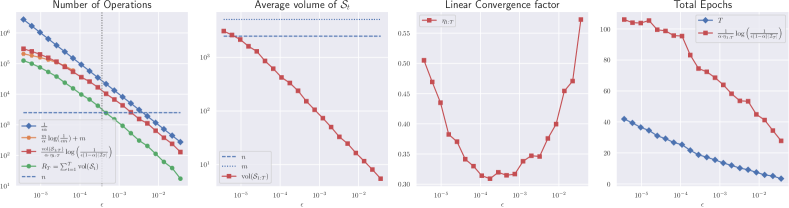
Figure 8: The illustration of operations on the Cora dataset. We run FIFOPush$(\mathcal{S},\epsilon,\alpha,s)$ for $\alpha=0.1$ and $\epsilon\in\left[10^{-2},10^{2}\right]*\sqrt{\frac{1-\alpha}{1+\alpha}}/n$. Compared with the linear bound $1/\alpha\epsilon$ in Andersen et al. (2006) and power-iteration bound $\frac{m}{\alpha}\log\left(\frac{1}{\epsilon m}\right)+m$ provided in Wu et al. (2021), our bound is better and shows the “locality” property of FIFOPush. Note that the bound $\frac{m}{\alpha}\log\left(\frac{1}{\epsilon m}\right)+m$ only works when $\epsilon<1/2m$.

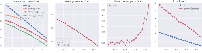
Figure 9: The illustration of our bound and parameters on the Cora dataset. We run FIFOPush$(\mathcal{S},\epsilon,\alpha,s)$ with $\alpha=0.5$.

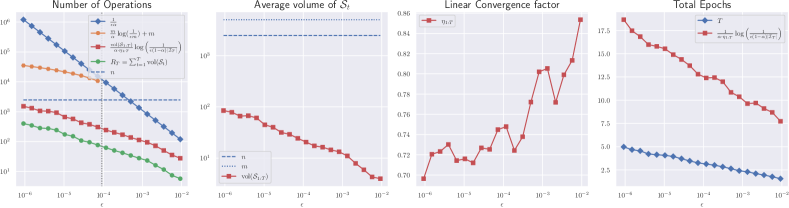
Figure 10: The illustration of our bound and parameters on the Cora dataset. We run FIFOPush$(\mathcal{S},\epsilon,\alpha,s)$ with $\alpha=0.9$.

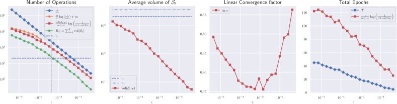
Figure 11: The illustration of operations on the Citeseer dataset. We run FIFOPush$(\mathcal{S},\epsilon,\alpha,s)$ for $\alpha=0.1$ and $\epsilon\in\left[10^{-2},10^{2}\right]*\sqrt{\frac{1-\alpha}{1+\alpha}}/n$. Compared with the linear bound $1/\alpha\epsilon$ in Andersen et al. (2006) and power-iteration bound $\frac{m}{\alpha}\log\left(\frac{1}{\epsilon m}\right)+m$ provided in Wu et al. (2021), our bound is better and shows the “locality” property of FIFOPush. Note that the bound $\frac{m}{\alpha}\log\left(\frac{1}{\epsilon m}\right)+m$ only works when $\epsilon<1/2m$.

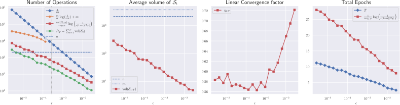
Figure 12: The illustration of our bound on the Citeseer dataset. We run FIFOPush$(\mathcal{S},\epsilon,\alpha,s)$ with $\alpha=0.5$.

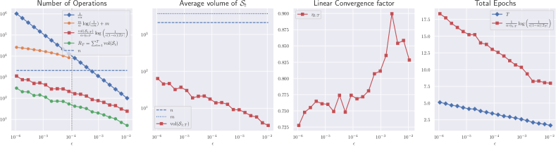
Figure 13: The illustration of our bound on the Citeseer dataset. We run FIFOPush$(\mathcal{S},\epsilon,\alpha,s)$ with $\alpha=0.9$.

A.3 Local linear convergence of FIFOPush for $(\alpha\bm{I}+\bm{D}-\bm{W})^{-1}$: The proof of Thm. 4.3

Given any $\alpha>0,\epsilon>0$, Algo. 5 is to approximate $(\alpha\bm{I}+\bm{D}-\bm{W})^{-1}$

Algorithm 5 $\textsc{FIFOPush}(\mathcal{G},\epsilon,\alpha,s)$ with a dummy node ${\color[rgb]{1,0,0}{\ddagger}}$

1:  Initialize: $\bm{r}_{t}=\tfrac{\bm{e}_{s}}{\alpha},\ \ \bm{x}_{t}=\bm{0},\ \ t=1,\ \ t^{\prime}=1$

2:  $\mathcal{Q}=[s,{\color[rgb]{1,0,0}{\ddagger}}]$          // At the initial stage, $\mathcal{Q}$ contains $s$ and a dummy node ${\color[rgb]{1,0,0}{\ddagger}}$.

3:  while $\mathcal{Q}\text{.size}()\neq 1$ do

4:     $u_{t^{\prime}}=\mathcal{Q}\text{.pop()}$

5:     if $u_{t^{\prime}}=={\color[rgb]{1,0,0}{\ddagger}}$ then

6:        $t=t+1$       // Nodes in $\mathcal{U}_{t}$ has been processed. Go to the next epoch.

7:        $\mathcal{Q}\text{.push}(u_{t^{\prime}})$

8:        continue

9:     end if

10:     if $r_{u_{t^{\prime}}}<\epsilon\cdot d_{u_{t^{\prime}}}$ then

11:        $t^{\prime}=t^{\prime}+1$        // $u_{t^{\prime}}$ is an “inactive” node

12:        continue

13:     end if

14:     $x_{u_{t^{\prime}}}=x_{u_{t^{\prime}}}+\frac{\alpha r_{u_{t^{\prime}}}}{\alpha+D_{u_{t^{\prime}}}}$    // $u_{t^{\prime}}$ is an “active” node

15:     for $v\in\mathcal{N}(u_{t^{\prime}})$ do

16:        $r_{v}=r_{v}+\frac{r_{u_{t^{\prime}}}w_{vu_{t^{\prime}}}}{\alpha+D_{u_{t^{\prime}}}}$

17:        if $v\notin\mathcal{Q}$ then

18:           $\mathcal{Q}\text{.push}(v)$

19:        end if

20:     end for

21:     $r_{u_{t^{\prime}}}=0$

22:     $t^{\prime}=t^{\prime}+1$

23:  end while

24:  Return $(\bm{x}_{t},\bm{r}_{t})$

Theorem 4.3 (Local convergence of FIFOPush for $\bm{X}_{\mathcal{L}}$).

Let $\bm{x}_{s}=\bm{X}_{\mathcal{L}}\bm{e}_{s}$ and run Aglo. 2 for $\bm{X}_{\mathcal{L}}$. For $s,i\in\mathcal{V}$, we have $\bm{x}_{s}=\bm{x}_{s,\epsilon}+\alpha\bm{X}_{\mathcal{L}}\bm{r}_{s,\epsilon},\text{ with }r_{s,\epsilon}(i)\leq[0,\epsilon d_{i}),\forall i\in\mathcal{V}$. The main operations of FIFOPush for $\bm{X}_{\mathcal{L}}$ is bounded as

$$R_{T}\leq\frac{\operatorname{vol}\left(\mathcal{S}_{1:T}\right)(\alpha+D_{\max})}{\alpha\cdot\eta_{1:T}}\log\left(\frac{C_{\alpha,T}}{\epsilon}\right),$$ (27)

where $\operatorname{vol}\left(\mathcal{S}_{1:T}\right)$ and $\eta_{1:T}$ are the same as in Thm. 4.2, $\eta_{t}\triangleq\tfrac{\sum_{u\in\mathcal{S}_{t}}d_{u}/(\alpha+D_{u})}{\sum_{v\in\mathcal{I}_{t}}d_{v}/(\alpha+D_{v})}$, $C_{\alpha,T}=1/\sum_{v\in\mathcal{I}_{T}}\frac{d_{u}w_{uv}}{\alpha+D_{u}}$, and $D_{\max}=\max_{v\in\operatorname{supp}\left(\bm{x}_{s,\epsilon}\right)}D_{v}$.

Proof.

The key of Alg. 5 is to maintain $\bm{x}_{t}$ and $\bm{r}_{t}$ so that $1/\alpha$ magnitudes will move from $\bm{r}$ to $\bm{x}$. For each active node $u_{t}$, $\bm{x}_{t}$ updates to $\tilde{{\bm{x}}}_{t+1}$ and $\bm{r}_{t}$ updates to $\tilde{{\bm{r}}}_{t+1}$ as the following

$$\tilde{\bm{x}}_{t+1} =\bm{x}_{t}+\frac{\alpha r_{u}}{\alpha+D_{u}}\bm{e}_{u}$$

$$\tilde{\bm{r}}_{t+1} =\bm{r}_{t}+\frac{r_{u}}{\alpha+D_{u}}\bm{W}\bm{e}_{u}-r_{u}\bm{e}_{u}=\bm{r}_{t}-\left(\bm{I}+\frac{\bm{D}-\bm{W}}{\alpha}\right)\frac{\alpha r_{u}}{\alpha+D_{u}}\bm{e}_{u}$$

$$\frac{\alpha r_{u}}{\alpha+D_{u}}\bm{e}_{u} =\left(\bm{I}+\frac{\bm{D}-\bm{W}}{\alpha}\right)^{-1}\left(\bm{r}_{t}-\tilde{\bm{r}}_{t+1}\right)$$

Bring back $t^{\prime}$ for $u$. After all active nodes in $t$-th epoch have been updated, we have

$${\bm{x}}_{t+1} =\bm{x}_{t}+\sum_{u_{t^{\prime}}\in\mathcal{S}_{t}}\frac{\alpha r_{u_{t^{\prime}}}}{\alpha+D_{u_{t^{\prime}}}}\bm{e}_{u_{t^{\prime}}}$$

$$=\bm{x}_{t}+\left(\bm{I}+\frac{\bm{D}-\bm{W}}{\alpha}\right)^{-1}\left(\bm{r}_{t}-{\bm{r}}_{t+1}\right)=\bm{x}_{1}+\left(\bm{I}+\frac{\bm{D}-\bm{W}}{\alpha}\right)^{-1}\sum_{i=1}^{t}\left(\bm{r}_{i}-{\bm{r}}_{i+1}\right)$$

$$=\left(\bm{I}+\frac{\bm{D}-\bm{W}}{\alpha}\right)^{-1}\left(\frac{\bm{e}_{s}}{\alpha}-{\bm{r}}_{t+1}\right),$$

where $\bm{r}_{t}=\tilde{\bm{r}}_{t}\rightarrow\tilde{\bm{r}}_{t^{\prime}+1}\rightarrow\tilde{\bm{r}}_{t^{\prime}+2}\rightarrow\cdots\tilde{\bm{r}}_{t^{\prime}+|\mathcal{S}_{t}|}={\bm{r}}_{t+1}$. Denote $\bm{x}_{t+1}$ as $\bm{x}_{s,\epsilon}$ and $\bm{r}_{t+1}$ as $\bm{r}_{s,\epsilon}$, then we have

$$\bm{x}_{s}=\bm{x}_{s,\epsilon}+\alpha\bm{X}\bm{r}_{s,\epsilon}.$$ (28)

After the $T$-th epoch finished, $\mathcal{I}_{T+1}=\operatorname{supp}\left(\bm{r}_{s,\epsilon}\right)$. For each $v\in\mathcal{I}_{T+1}$, note that there exists at least one of its neighbor $u\in\mathcal{N}{(v)}$ such that $r_{u}\geq\epsilon\cdot d_{u}$ had happened in a previous active iteration.

$$\forall v\in\mathcal{I}_{T+1},\quad\frac{r_{u}w_{uv}}{\alpha+D_{u}}\geq\frac{\epsilon d_{u}w_{uv}}{\alpha+D_{u}}\triangleq\tilde{r}_{v},$$

where $\tilde{r}_{v}$ is the residual pushed into $v$ but never popped out; hence $\sum_{v\in\mathcal{I}_{T+1}}\tilde{r}_{v}$ is an estimate of $\|\bm{r}_{T+1}\|_{1}$ from bottom. That is

$$\sum_{v\in\mathcal{I}_{T+1}}\tilde{r}_{v}=\sum_{v\in\mathcal{I}_{T+1}}\frac{\epsilon d_{u}w_{uv}}{\alpha+D_{u}}\leq\|\bm{r}_{T+1}\|_{1}.$$ (29)

The operation bounds are similar to that of 4.2. Note that for each epoch, the updates of $\bm{r}$ satisfies

$$\|\bm{r}_{t}\|_{1}-\|\bm{r}_{t+1}\|_{1}\geq\sum_{u_{t^{\prime}}\in\mathcal{S}_{t}}\frac{\alpha r_{u_{t^{\prime}}}}{\alpha+D_{u_{t^{\prime}}}}.$$ (30)

By the condition, we have $\forall u_{t^{\prime}}\in\mathcal{S}_{t},r_{u_{t^{\prime}}}\geq\epsilon\cdot d_{u_{t^{\prime}}},\forall v\in\mathcal{I}_{t}\backslash\mathcal{S}_{t},0<r_{t}(v)<\epsilon\cdot d_{v}$. Summation above inequalities over all active $u_{t^{\prime}}$ and inactive $v$, multiply $\tfrac{\alpha}{\alpha+D_{u}}$ on both sides, we have

$$\frac{\sum_{u_{t^{\prime}}\in\mathcal{S}_{t}}\frac{\alpha r_{u_{t^{\prime}}}}{\alpha+D_{u_{t^{\prime}}}}}{\sum_{u_{t^{\prime}}\in\mathcal{S}_{t}}\frac{\alpha d_{u_{t^{\prime}}}}{\alpha+D_{u_{t^{\prime}}}}}\geq\epsilon>\frac{\sum_{v\in\mathcal{I}_{t}\backslash\mathcal{S}_{t}}\frac{\alpha r_{v}}{\alpha+D_{v}}}{\sum_{v\in\mathcal{I}_{t}\backslash\mathcal{S}_{t}}\frac{\alpha d_{v}}{\alpha+D_{v}}},$$

which indicates

$$\frac{\sum_{u_{t^{\prime}}\in\mathcal{S}_{t}}\frac{\alpha r_{u_{t^{\prime}}}}{\alpha+D_{u_{t^{\prime}}}}}{\sum_{u_{t^{\prime}}\in\mathcal{S}_{t}}\frac{\alpha d_{u_{t^{\prime}}}}{\alpha+D_{u_{t^{\prime}}}}}\geq\frac{\sum_{u_{t^{\prime}}\in\mathcal{S}_{t}}\frac{\alpha r_{u_{t^{\prime}}}}{\alpha+D_{u_{t^{\prime}}}}+\sum_{v\in\mathcal{I}_{t}\backslash\mathcal{S}_{t}}\frac{\alpha r_{v}}{\alpha+D_{v}}}{\sum_{u_{t^{\prime}}\in\mathcal{S}_{t}}\frac{\alpha d_{u_{t^{\prime}}}}{\alpha+D_{u_{t^{\prime}}}}+\sum_{v\in\mathcal{I}_{t}\backslash\mathcal{S}_{t}}\frac{\alpha d_{v}}{\alpha+D_{v}}}\geq\frac{\frac{\alpha}{\alpha+D_{\max}}\|\bm{r}_{t}\|_{1}}{\sum_{v\in\mathcal{I}_{t}}\frac{\alpha d_{v}}{\alpha+D_{v}}}$$ (31)

where the last equality is due to the fact that $\mathcal{I}_{t}$ indexes all nonzero entries of $\bm{r}_{t}$, i.e., $\|\bm{r}_{t}\|_{1}=\sum_{v\in\mathcal{I}_{t}}r_{t}(v)$. Combine (30) and (31), for $t=1,2,\ldots,T$, we have

$$\|\bm{r}_{t+1}\|_{1}<\left(1-\frac{\alpha}{\alpha+D_{\max}}\frac{\sum_{u\in\mathcal{S}_{t}}d_{u}/(\alpha+D_{u})}{\sum_{v\in\mathcal{I}_{t}}d_{v}/(\alpha+D_{v})}\right)\|\bm{r}_{t}\|_{1}.$$

From $t=1$ to $t=T$, we obtain

$$\sum_{v\in\mathcal{I}_{T+1}}\frac{\epsilon d_{u}w_{uv}}{\alpha+D_{u}}\leq\|\bm{r}_{T+1}\|_{1}\leq\prod_{t=1}^{T}\left(1-\frac{\alpha}{\alpha+D_{\max}}\frac{\sum_{u\in\mathcal{S}_{t}}d_{u}/(\alpha+D_{u})}{\sum_{v\in\mathcal{I}_{t}}d_{v}/(\alpha+D_{v})}\right).$$

Denote $C_{T}=1/\sum_{v\in\mathcal{I}_{T+1}}\frac{d_{u}w_{uv}}{\alpha+D_{u}}$. Take the logarithm on both sides of the above and we reach

$$\frac{\alpha}{\alpha+D_{\max}}\sum_{t=1}^{T}\frac{\sum_{u\in\mathcal{S}_{t}}d_{u}/(\alpha+D_{u})}{\sum_{v\in\mathcal{I}_{t}}d_{v}/(\alpha+D_{v})}\leq\log\left(\frac{C_{T}}{\epsilon}\right).$$ (32)

Then by (32), the total number of epochs can be bounded by $T\leq\tfrac{\alpha+D_{\max}}{\alpha\cdot{\eta}_{1:T}}\log\left(\tfrac{C_{T}}{\epsilon}\right)$. The total operations for processing active nodes is $R_{T}=\sum_{t=1}^{T}\operatorname{vol}\left(\mathcal{S}_{t}\right)$, which is bounded as

$$R_{T}\leq\frac{(\alpha+D_{\max})\operatorname{vol}\left(\mathcal{S}_{1:T}\right)}{\alpha\cdot{\eta}_{1:T}}\log\left(\frac{C_{T}}{\epsilon}\right).$$

∎

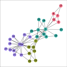
(a) Labeled Karate

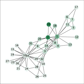
(b) $\bm{x}_{22,\epsilon}$ on $\mathcal{G}$

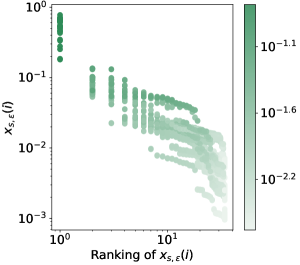
(c) Power law of $\bm{X}_{\epsilon}$

Figure 14: Power law distribution of $\bm{X}_{\mathcal{L}}\bm{e}_{s}$ on Karate graph (Girvan & Newman, 2002). (a) The Karate contains 34 nodes and 78 edges forming four communities ($w_{uv}$ is the 2-dimensional Euclidean distance.); (b) We run FIFOPush$(\mathcal{G},\epsilon,\alpha,s)$ on $s=22$ with $\alpha=0.85$ and $\epsilon=10^{-12}$. Neighbors of $s=22$ have large magnitudes of $\bm{x}_{s}$; (We changed the magnitude of $\bm{x}_{s}(22)$ to the largest magnitude of rest for better visibility.) (c) The power law distribution of entries of $\bm{x}_{s}$ for all 34 nodes.

A.4 Approximation kernels and their residuals

Table 3: The parameterized graph kernel matrices with their kernel approximation

ID	$\alpha$	Basic Kernel Presentation	Approximation $\bm{M}_{\epsilon}$	Residual Matrix $\bm{E}_{\epsilon}$
1	$\frac{\lambda}{n}$	$\bm{M}_{\lambda,\beta}=2\lambda\bm{X}_{\mathcal{L}}$	$2\lambda\bm{X}_{\epsilon}$	$2\lambda\alpha\bm{X}_{\mathcal{\bm{L}}}\bm{R}_{\epsilon}$
2	$\frac{\lambda}{n+\lambda}$	$\bm{M}_{\lambda,\beta}=2n{\bm{D}}^{-1/2}\bm{X}_{\bm{L}}{\bm{D}}^{1/2}$	$2n\bm{D}^{-1/2}{\bm{X}}_{\epsilon}\bm{D}^{1/2}$	$2n\bm{D}^{-1/2}\bm{X}_{\bm{L}}\bm{R}_{\epsilon}\bm{D}^{1/2}$
3	$\frac{n+\lambda-\beta n}{n+\lambda}$	$\bm{M}_{\lambda,\beta}=\frac{2\lambda n}{n+\lambda-\beta n}{\bm{D}}^{-1/2}\bm{X}_{\bm{L}}{\bm{D}}^{1/2}$	$\frac{2\lambda n}{n+\lambda-\beta n}\bm{D}^{-1/2}{\bm{X}}_{\epsilon}\bm{D}^{1/2}$	$\frac{2\lambda n}{n+\lambda-\beta n}\bm{D}^{-1/2}\bm{X}_{\bm{L}}\bm{R}_{\epsilon}\bm{D}^{1/2}$
4	$\frac{n\beta+\lambda}{n}$	$\bm{M}_{\lambda,\beta}=2\lambda{\bm{S}}^{-1/2}\bm{X}_{\mathcal{L}}{\bm{S}}^{1/2}$	$2\lambda\bm{S}^{-1/2}\bm{X}_{\epsilon}\bm{S}^{1/2}$	$2\lambda\bm{S}^{-1/2}\alpha\bm{X}_{\mathcal{\bm{L}}}\bm{R}_{\epsilon}\bm{S}^{1/2}$
5	$2\lambda$	$\bm{M}_{\lambda,\beta}=\left(\frac{\bm{S}^{1/2}}{4n\lambda}+\frac{\beta\bm{S}^{-1/2}}{4\lambda^{2}}\right)^{-1}\bm{X}_{\mathcal{L}}{\bm{S}}^{1/2}$	$\left(\frac{\bm{S}^{1/2}}{4n\lambda}+\frac{\beta\bm{S}^{-1/2}}{4\lambda^{2}}\right)^{-1}\bm{X}_{\epsilon}{\bm{S}}^{1/2}$	$\alpha\left(\frac{\bm{S}^{1/2}}{4n\lambda}+\frac{\beta\bm{S}^{-1/2}}{4\lambda^{2}}\right)^{-1}\bm{X}_{\mathcal{L}}\bm{R}_{\epsilon}{\bm{S}}^{1/2}$
6	$\beta+\frac{\lambda}{n}$	$\bm{M}_{\lambda,\beta}=2\lambda\bm{X}_{\mathcal{L}}\left(\bm{I}-\frac{b\bm{1}\bm{1}^{\top}}{\alpha+nb}\right)$	$\bm{M}_{\lambda,\beta}=2\lambda\bm{X}_{\epsilon}\left(\bm{I}-\frac{b\bm{1}\bm{1}^{\top}}{\alpha+nb}\right)$	$2\lambda\alpha\bm{X}_{\mathcal{L}}\bm{R}_{\epsilon}\left(\bm{I}-\frac{b\bm{1}\bm{1}^{\top}}{\alpha+nb}\right)$

Recall two types of matrix presentation and their approximations

$$\bm{X}_{\bm{L}} =\alpha(\bm{I}-(1-\alpha)\bm{W}\bm{D}^{-1})^{-1}=\bm{X}_{\epsilon}+\bm{X}_{\bm{L}}\bm{R}_{\epsilon},$$

$$\bm{X}_{\mathcal{\bm{L}}} =(\alpha\bm{I}+\bm{D}-\bm{W})^{-1}=\bm{X}_{\epsilon}+\alpha\bm{X}_{\mathcal{\bm{L}}}\bm{R}_{\epsilon}.$$

Based on the above lemmas, we list the approximation kernels in Tab. 3. $\bm{X}_{\epsilon}=[\bm{x}_{1,\epsilon},\bm{x}_{2,\epsilon},\ldots,\bm{x}_{n,\epsilon}]$ be the matrix obtained by applying FIFOPush as described in Algorithm 2. We only show the first two cases to see how to represent these matrices in terms of $\bm{X}_{\epsilon}$ and $\bm{R}_{\epsilon}$. For example, in the first case, we have

$$\bm{M}_{\lambda,\beta}=\left(\frac{\bm{D}-\bm{W}}{2\lambda}+\frac{\bm{I}_{n}}{2n}\right)^{-1}=2\lambda\left(\alpha\bm{I}_{n}+{\mathcal{\bm{L}}}\right)^{-1}=2\lambda\bm{X}_{\mathcal{\bm{L}}}=2\lambda(\bm{X}_{\epsilon}+\alpha\bm{X}_{\mathcal{\bm{L}}}\bm{R}_{\epsilon}).$$

For the second case, the kernel matrix can be rewritten as $\bm{M}=2n{\bm{D}}^{-1/2}\bm{X}_{\bm{L}}{\bm{D}}^{1/2}$. By Lemma A.1, we have

$$\bm{X}_{\bm{L}} ={\bm{X}}_{\epsilon}+\bm{X}_{\bm{L}}\bm{R}_{\epsilon}$$

$$2n\bm{D}^{-1/2}\bm{X}_{\bm{L}}\bm{D}^{1/2} =2n\bm{D}^{-1/2}({\bm{X}}_{\epsilon}+\bm{X}_{\bm{L}}\bm{R}_{\epsilon})\bm{D}^{1/2}$$

$$\bm{M} =2n\bm{D}^{-1/2}{\bm{X}}_{\epsilon}\bm{D}^{1/2}+2n\bm{D}^{-1/2}\bm{X}_{\bm{L}}\bm{R}_{\epsilon}\bm{D}^{1/2}$$

$$\bm{M} =2n\bm{D}^{-1/2}{\bm{X}}_{\epsilon}\bm{D}^{1/2}+\bm{M}\bm{D}^{-1/2}\bm{R}_{\epsilon}\bm{D}^{1/2}.$$

For all these cases, we have the relationship that $\bm{M}=\bm{M}_{\epsilon}+\bm{E}_{\epsilon}$.

Appendix B Eigenvalues of $\bm{M}_{\lambda,\beta}$ and quadratic approximation guarantees of $\bm{M}_{\epsilon}$

$\bm{M}_{\lambda,\beta}$ is the matrix we want to approximate. Recall $\bm{X}_{\epsilon}$ be the approximated matrix by FIFOPush. $\bm{M}_{\epsilon}$ be the matrix built upon $\bm{X}_{\epsilon}$ (See 3rd column of Table 3). In the following, we will construct the relaxation function based on $\bm{M}_{\epsilon}$. The following lemma shows that if $\bm{M}_{\epsilon}$ is a good approximation of $\bm{M}$ then we can define a relaxation function based $\bm{M}_{\epsilon}$. Before we present the theorem, let us characterize the eigenvalues of $\bm{X}_{\bm{L}}$ and $\bm{X}_{\mathcal{L}}$.

Lemma B.1.

The eigenvalue functions of these two basic kernel matrices $\bm{X}_{\bm{L}}$ and $\bm{X}_{\mathcal{\bm{L}}}$ satisfy

$$\lambda(\bm{X}_{\bm{L}})=\lambda\left(\alpha\left(\bm{I}-(1-\alpha)\bm{W}\bm{D}^{-1}\right)^{-1}\right) \in\left[\frac{\alpha}{2-\alpha},1\right],$$

$$\lambda(\bm{X}_{\mathcal{\bm{L}}})=\lambda\left(\left(\alpha\bm{I}+\bm{D}-\bm{W}\right)^{-1}\right) \in\left[\frac{1}{\alpha+2D_{\max}},\frac{1}{\alpha}\right],$$

where $D_{\max}$ is the maximum weighted degree among $\mathcal{V}$. For $\bm{X}_{\bm{L}}$, we assume $\alpha\in(0,1)$, and for $\bm{X}_{\mathcal{\bm{L}}}$, $\alpha>0$.

Proof.

Notice that since the magnitude of the eigenvalues of the column stochastic matrix $\bm{W}\bm{D}^{-1}$ is bounded by $1$, i.e., $|\lambda(\bm{W}\bm{D}^{-1})|\leq 1$, then we have

$$\lambda(\bm{I}-(1-\alpha)\bm{W}\bm{D}^{-1}) \in\left[\alpha,2-\alpha\right]$$

$$\lambda\left(\left(\bm{I}-(1-\alpha)\bm{W}\bm{D}^{-1}\right)^{-1}\right) \in\left[\frac{1}{2-\alpha},\frac{1}{\alpha}\right]$$

$$\lambda\left(\alpha\left(\bm{I}-(1-\alpha)\bm{W}\bm{D}^{-1}\right)^{-1}\right) \in\left[\frac{\alpha}{2-\alpha},1\right].$$

Hence, we have the first bounding inequality. To show the second inequality, notice that if $\bm{x}$ is an eigenvalue of $\bm{D}-\bm{W}$, then

$$(\bm{D}-\bm{W})\bm{x} =\lambda\bm{x}$$

$$\bm{x}^{\top}(\bm{D}-\bm{W})\bm{x} =\lambda\bm{x}^{\top}\bm{x}$$

$$\sum_{(u,v)\in\mathcal{E}}w_{uv}(x_{u}-x_{v})^{2} =\lambda\bm{x}^{\top}\bm{x}.$$

Hence $\lambda\geq 0$, and the lower bound is achieved when $\bm{x}=\bm{1}$. On the other hand, a well-known result (Anderson Jr & Morley, 1985) of the upper bound is

$$\lambda(\bm{D}-\bm{W})\leq\max_{(u,v)\in\mathcal{E}}D_{u}+D_{v}\leq 2D_{\max}.$$

where $D_{\max}$ is the maximum weighted degree among all nodes. It follows that

$$\lambda(\bm{D}-\bm{W}) \in\left[0,2D_{\max}\right]$$

$$\lambda(\alpha\bm{I}+\bm{D}-\bm{W}) \in\left[\alpha,\alpha+2D_{\max}\right]$$

$$\lambda\left(\left(\alpha\bm{I}+\bm{D}-\bm{W}\right)^{-1}\right) \in\left[\frac{1}{\alpha+2D_{\max}},\frac{1}{\alpha}\right].$$

∎

Lemma B.2.

Let $\bm{M}$ be a symmetric positive definite matrix and $\bm{D}$ be a positive diagonal matrix. Then, for any nonnegative real matrix $\bm{R}\in{\mathbb{R}}_{+}^{n\times n}$ and $\bm{x}\neq\bm{0}$, we have

$$\frac{1}{2}\frac{\bm{x}^{\top}(\bm{M}\bm{D}^{-1/2}\bm{R}\bm{D}^{1/2}+\bm{D}^{1/2}\bm{R}^{\top}\bm{D}^{-1/2}\bm{M})\bm{x}}{\bm{x}^{\top}\bm{M}\bm{x}}\leq\|\bm{D}^{-1/2}\bm{R}\bm{D}^{1/2}\|_{2}.$$ (33)

Proof.

Since $\bm{M}$ is a symmetric positive definite matrix, one can write $\bm{M}=\bm{B}\bm{B}^{\top}$ and $\bm{B}$ are invertible. The decomposition of $\bm{M}$ is $\bm{M}=\bm{Q}\bm{\Lambda}\bm{Q}^{\top}=\bm{Q}\bm{\Lambda}^{1/2}\bm{\Lambda}^{1/2}\bm{Q}^{\top}$ where we can let $\bm{B}=\bm{Q}\bm{\Lambda}^{1/2}$ and $\bm{Q}$ is an orthonormal matrix. Let $\bm{y}=\bm{B}^{\top}\bm{x}$, then $\bm{x}^{\top}\bm{M}\bm{x}=\bm{y}^{\top}\bm{y}$ and $\bm{x}=(\bm{B}^{\top})^{-1}\bm{y}$. Let $\bm{Z}=\bm{D}^{-1/2}\bm{R}\bm{D}^{1/2}$. We have

$$(*) =\frac{1}{2}\frac{\bm{x}^{\top}\left(\bm{M}\bm{D}^{-1/2}\bm{R}\bm{D}^{1/2}+\bm{D}^{1/2}\bm{R}^{\top}\bm{D}^{-1/2}\bm{M}\right)\bm{x}}{\bm{x}^{\top}\bm{M}\bm{x}}$$

$$=\frac{1}{2}\frac{\bm{x}^{\top}\left(\bm{M}\bm{Z}+\bm{Z}^{\top}\bm{M}\right)\bm{x}}{\bm{y}^{\top}\bm{y}}$$

$$=\frac{1}{2}\frac{\bm{y}^{\top}\bm{B}^{-1}\left(\bm{B}\bm{B}^{\top}\bm{Z}+\bm{Z}^{\top}\bm{B}\bm{B}^{\top}\right)(\bm{B}^{\top})^{-1}\bm{y}}{\bm{y}^{\top}\bm{y}}$$

$$=\frac{1}{2}\frac{\bm{y}^{\top}\left(\bm{B}^{\top}\bm{Z}(\bm{B}^{\top})^{-1}+\bm{B}^{-1}\bm{Z}^{\top}\bm{B}\right)\bm{y}}{\bm{y}^{\top}\bm{y}}$$

$$=\frac{1}{2}\frac{\bm{y}^{\top}\left(\bm{\Lambda}^{1/2}\bm{Q}^{\top}\bm{Z}(\bm{Q}^{\top})^{-1}\bm{\Lambda}^{-1/2}+{\bm{\Lambda}}^{-1/2}\bm{Q}^{-1}\bm{Z}^{\top}\bm{Q}{\bm{\Lambda}}^{1/2}\right)\bm{y}}{\bm{y}^{\top}\bm{y}}$$

$$\leq\frac{1}{2}\left\|\bm{\Lambda}^{1/2}\bm{Q}^{\top}\bm{Z}(\bm{Q}^{\top})^{-1}\bm{\Lambda}^{-1/2}+{\bm{\Lambda}}^{-1/2}\bm{Q}^{-1}\bm{Z}^{\top}\bm{Q}{\bm{\Lambda}}^{1/2}\right\|_{2}$$

where the inequality follows Rayleigh’s quotient property, that is, any matrix norm bounds the maximal absolute eigenvalue, and the spectral radius is less than any matrix norm. Denoting $\mathbf{A}=\mathbf{Q}^{\top}\mathbf{Z}(\mathbf{Q}^{\top})^{-1}$, we may write

$$2(*) = \left\|\bm{\Lambda}^{1/2}\bm{Q}^{\top}\bm{Z}(\bm{Q}^{\top})^{-1}\bm{\Lambda}^{-1/2}+{\bm{\Lambda}}^{-1/2}\bm{Q}^{-1}\bm{Z}^{\top}\bm{Q}{\bm{\Lambda}}^{1/2}\right\|_{2}$$

$$= \max_{u|\|u\|_{2}=1}|u^{T}\bm{\Lambda}^{1/2}\bm{A}\bm{\Lambda}^{-1/2}u+u^{T}{\bm{\Lambda}}^{-1/2}\bm{A}{\bm{\Lambda}}^{1/2}u|_{2}$$

and denoting $\bm{w}=\bm{\Lambda}^{1/2}\bm{u},\bm{v}=\bm{\Lambda}^{-1/2}\bm{u}$

$$|\bm{u}^{\top}\bm{\Lambda}^{1/2}\bm{A}\bm{\Lambda}^{-1/2}\bm{u}+\bm{u}^{\top}{\bm{\Lambda}}^{-1/2}\bm{A}{\bm{\Lambda}}^{1/2}\bm{u}| =2|\bm{w}^{\top}\bm{A}\bm{v}|=2|\operatorname{tr}\left(\bm{v}\bm{w}^{\top}\bm{A}\right)| \overset{(\circ)}{\leq}2|\bm{w}^{\top}\bm{v}|\|\bm{A}\|_{2},$$

where the inequality $(\circ)$ is due to Holder’s $p=1$ inequality applied to the matrix singular values. Since $\bm{w}^{\top}\bm{v}=\bm{u}^{\top}\bm{u}=1$, $(*)\leq\|\bm{Q}^{\top}\bm{Z}(\bm{Q}^{T})^{-1}\|_{2}=\|\bm{Z}\|_{2}$. ∎

The next lemma shows FIFOPush provides good approximations. Here we only show Instance 3 and Instance 4.

Lemma B.3.

Let ${\bm{X}}_{\epsilon}$ and ${\bm{R}}_{\epsilon}$ be the approximate and the residual matrix obtained by applying $\textsc{FIFOPush}(\mathcal{G},\epsilon,\alpha,s)$ $\forall s\in\mathcal{V}$. Then we have the following inequalities

$$\bm{x}^{\top}\left(\frac{\bm{M}_{\epsilon}+\bm{M}_{\epsilon}^{\top}}{2}\right)\bm{x} \geq\bm{x}^{\top}\bm{M}\bm{x}\left(1-\|\bm{D}^{-1/2}\bm{R}_{\epsilon}\bm{D}^{1/2}\|_{2}\right)\text{ for }\bm{M}=\frac{2\lambda n}{n+\lambda-\beta n}{\bm{D}}^{-1/2}\bm{X}_{\bm{L}}{\bm{D}}^{1/2},$$

$$\bm{x}^{\top}\left(\frac{\bm{M}_{\epsilon}+\bm{M}_{\epsilon}^{\top}}{2}\right)\bm{x} \geq\bm{x}^{\top}\bm{M}\bm{x}\left(1-\|\bm{S}^{-1/2}\bm{R}_{\epsilon}\bm{S}^{1/2}\|_{2}\right)\text{ for }\bm{M}=2\lambda\bm{S}^{-1/2}\bm{X}_{\mathcal{L}}{\bm{D}}^{1/2}.$$

Proof.

The inequality is trivially true when $\bm{x}=\bm{0}$. In the rest, we assume $\bm{x}\neq\bm{0}$. For ease of notation, we simply write $\bm{M}=\bm{M}_{\lambda,\beta}$, and

$$\bm{M}=\bm{M}_{\epsilon}+\bm{E}_{\epsilon},\qquad\bm{X}_{\bm{L}}=\bm{X}_{\epsilon}+\bm{X}_{\bm{L}}\bm{R}_{\epsilon}.$$

We consider two parameterized kernels as follows

1. $\bm{M}=c{\bm{D}}^{-1/2}\bm{X}_{\bm{L}}{\bm{D}}^{1/2}$ where $c=\frac{2\lambda n}{n+\lambda-\beta n}$. Here,

   $$\bm{X}_{\bm{L}}=\alpha(\bm{I}-(1-\alpha)\bm{W}\bm{D}^{-1})^{-1},\qquad\bm{M}_{\epsilon}=c\bm{D}^{-1/2}{\bm{X}}_{\epsilon}\bm{D}^{1/2},\qquad\bm{E}_{\epsilon}=c\bm{D}^{-1/2}\bm{X}_{\bm{L}}\bm{R}_{\epsilon}\bm{D}^{1/2}.$$

   We have

   $$\bm{x}^{\top}\bm{M}\bm{x} =\bm{x}^{\top}\bm{M}_{\epsilon}\bm{x}+\bm{x}^{\top}\bm{E}_{\epsilon}\bm{x}$$

   $$=\bm{x}^{\top}\left(\frac{\bm{M}_{\epsilon}+\bm{M}_{\epsilon}}{2}^{\top}\right)\bm{x}+\frac{1}{2}\bm{x}^{\top}\left(\bm{M}\bm{D}^{-1/2}\bm{R}_{\epsilon}\bm{D}^{1/2}+\bm{D}^{1/2}\bm{R}_{\epsilon}^{\top}\bm{D}^{-1/2}\bm{M}\right)\bm{x}$$

   $$=\bm{x}^{\top}\left(\frac{\bm{M}_{\epsilon}+\bm{M}_{\epsilon}}{2}^{\top}\right)\bm{x}+\bm{x}^{\top}\bm{M}\bm{x}\cdot\frac{\bm{x}^{\top}\left(\bm{M}\bm{D}^{-1/2}\bm{R}_{\epsilon}\bm{D}^{1/2}+\bm{D}^{1/2}\bm{R}_{\epsilon}^{\top}\bm{D}^{-1/2}\bm{M}\right)\bm{x}}{2\bm{x}^{\top}\bm{M}\bm{x}}$$

   $$\leq\bm{x}^{\top}\left(\frac{\bm{M}_{\epsilon}+\bm{M}_{\epsilon}}{2}^{\top}\right)\bm{x}+\bm{x}^{\top}\bm{M}\bm{x}\cdot\|\bm{D}^{-1/2}\bm{R}\bm{D}^{1/2}\|_{2},$$

   where the last inequality follows from Lemma 33 of (33). Rearrange the above; we finish the first case.

2. $\bm{M}=2\lambda{\bm{S}}^{-1/2}\bm{X}_{\mathcal{L}}{\bm{S}}^{1/2}$. Here,

   $$\bm{X}_{\mathcal{\bm{L}}}=(\alpha\bm{I}+\bm{D}-\bm{W})^{-1}\qquad\bm{M}_{\epsilon}=2\lambda\bm{S}^{-1/2}\bm{X}_{\epsilon}\bm{S}^{1/2},\qquad\bm{E}_{\epsilon}=2\lambda\bm{S}^{-1/2}\alpha\bm{X}_{\mathcal{\bm{L}}}\bm{R}_{\epsilon}\bm{S}^{1/2}.$$

   Then

   $$\bm{x}^{\top}\bm{M}\bm{x} =\bm{x}^{\top}(\bm{M}_{\epsilon}+\bm{E}_{\epsilon})\bm{x}$$

   $$=\bm{x}^{\top}\left(\frac{\bm{M}_{\epsilon}+\bm{M}_{\epsilon}}{2}^{\top}\right)\bm{x}+\frac{\alpha}{2}\bm{x}^{\top}\left(\bm{M}\bm{S}^{-1/2}\bm{R}_{\epsilon}\bm{S}^{1/2}+\bm{S}^{1/2}\bm{R}_{\epsilon}^{\top}\bm{S}^{-1/2}\bm{M}\right)\bm{x}$$

   $$=\bm{x}^{\top}\left(\frac{\bm{M}_{\epsilon}+\bm{M}_{\epsilon}}{2}^{\top}\right)\bm{x}+\bm{x}^{\top}\bm{M}\bm{x}\cdot\frac{\alpha\bm{x}^{\top}\left(\bm{M}\bm{S}^{-1/2}\bm{R}_{\epsilon}\bm{S}^{1/2}+\bm{S}^{1/2}\bm{R}_{\epsilon}^{\top}\bm{S}^{-1/2}\bm{M}\right)\bm{x}}{2\bm{x}^{\top}\bm{M}\bm{x}}$$

   $$\leq\bm{x}^{\top}\left(\frac{\bm{M}_{\epsilon}+\bm{M}_{\epsilon}}{2}^{\top}\right)\bm{x}+\bm{x}^{\top}\bm{M}\bm{x}\cdot\alpha\|\bm{S}^{-1/2}\bm{R}\bm{S}^{1/2}\|_{2},$$

   by applying Lemma 33 with $\bm{D}=\bm{S}^{1/2}$.

Rearrange the above; we finish the proof. ∎

Remark B.4.

The above theorem allows us to control the error of $\bm{M}_{\epsilon}$. Next, we show that if $\frac{\bm{M}_{\epsilon}+\bm{M}_{\epsilon}^{\top}}{2}$ is a positive semidefinite matrix, then we can find an approximate relaxation function.

Lemma B.5.

Let $\bm{G}^{t}=[\bm{\nabla}_{1},\ldots,\bm{\nabla}_{t},\bm{0},\ldots,\bm{0}]\in\mathbb{R}^{k\times n}$ with $\|\bm{\nabla}_{t}\|_{2}\leq D$. Let $\bm{M}_{\epsilon}$ be the approximation built upon $\bm{X}_{\epsilon}$ as defined in Table 3 such that $\left(\frac{\bm{M}_{\epsilon}+\bm{M}_{\epsilon}^{\top}}{2}\right)$ is positive semidefinite. If we provide the following score

$$\bm{\psi}_{t}=-\frac{\bm{G}^{t-1}(\bm{M}_{\epsilon})_{:,t}+\bm{G}^{t-1}(\bm{M}_{\epsilon})_{t,:}^{\top}}{\sqrt{Q_{t-1}+D^{2}\sum_{j=t}^{n}(M_{\epsilon})_{j,j}}},$$

where $Q_{t}\triangleq\sum_{i=1}^{k}\left(\bm{G}_{i}^{t}\right)^{\top}\left(\frac{\bm{M}_{\epsilon}+\bm{M}_{\epsilon}^{\top}}{2}\right)\bm{G}_{i}^{t}$, then the relaxation function defined

$$\operatorname{Rel}_{t}\left(\bm{\nabla}_{1},\ldots,\bm{\nabla}_{t};\bm{M}_{\epsilon}\right)\triangleq\sqrt{Q_{t}+D^{2}\sum_{j=t+1}^{n}(M_{\epsilon})_{j,j}}$$

is admissible; that is, for all $t=1,2,\ldots,n$,

$$\inf_{\bm{\psi}_{t}\in\mathbb{R}^{k}}\sup_{\|\bm{\nabla}_{t}\|\leq D}\left\{\bm{\nabla}_{t}^{\top}\bm{\psi}_{t}+\operatorname{Rel}_{t}\left(\bm{\nabla}_{1}\ldots,\bm{\nabla}_{t};\bm{M}_{\epsilon}\right)\right\}\leq\operatorname{Rel}_{t-1}(\bm{\nabla}_{1},\ldots,\bm{\nabla}_{t-1};\bm{M}_{\epsilon})$$

where $\operatorname{Rel}_{0}(\emptyset;\bm{M}_{\epsilon})=\sqrt{D^{2}\cdot\operatorname{tr}\left(\bm{M}_{\epsilon}\right)}$.

Proof.

Define $\bm{b}_{i}^{t}=\left[0,\ldots,\nabla_{t}(i),0,\ldots,0\right]^{\top}\in{\mathbb{R}}^{n}$. Note that $(\bm{G}_{i}^{t})^{\top}=(\bm{G}_{i}^{t-1}+\bm{b}_{i}^{t})^{\top}$ where $i=1,2,\ldots,k$ indexing label id and $t=1,2,\ldots,n$ indexing node id. We define the following quadratic based on $\bm{M}_{\epsilon}$

$$Q_{t} \triangleq\sum_{i=1}^{k}\left(\bm{G}_{i}^{t}\right)^{\top}\left(\frac{\bm{M}_{\epsilon}+\bm{M}_{\epsilon}^{\top}}{2}\right)\bm{G}_{i}^{t}$$

$$=\sum_{i=1}^{k}\left(\bm{G}_{i}^{t-1}+\bm{b}_{i}^{t}\right)^{\top}\left(\frac{\bm{M}_{\epsilon}+\bm{M}_{\epsilon}^{\top}}{2}\right)\left(\bm{G}_{i}^{t-1}+\bm{b}_{i}^{t}\right)$$

$$=\sum_{i=1}^{k}\left\{\left(\bm{G}_{i}^{t-1}\right)^{\top}\left(\frac{\bm{M}_{\epsilon}+\bm{M}_{\epsilon}^{\top}}{2}\right)\bm{G}_{i}^{t-1}+\left(\bm{G}_{i}^{t-1}\right)^{\top}\left(\bm{M}_{\epsilon}+\bm{M}_{\epsilon}^{\top}\right)\bm{b}_{i}^{t}+(\bm{b}_{t}^{i})^{\top}\left(\frac{\bm{M}_{\epsilon}+\bm{M}_{\epsilon}^{\top}}{2}\right)\bm{b}_{t}^{i}\right\}$$

$$=Q_{t-1}+\sum_{i=1}^{k}\left\{\left(\bm{G}_{i}^{t-1}\right)^{\top}\bm{M}_{\epsilon}\bm{b}_{i}^{t}+(\bm{b}_{i}^{t})^{\top}\bm{M}_{\epsilon}\bm{G}_{i}^{t-1}+\left(\nabla_{t}(i)\right)^{2}(M_{\epsilon})_{t,t}\right\}$$

$$=Q_{t-1}+\sum_{i=1}^{k}\left(\nabla_{t}(i)((\bm{G}_{i}^{t-1})^{\top}(\bm{M}_{\epsilon})_{:,t}+(\bm{M}_{\epsilon})_{t,:}^{\top}\bm{G}_{i}^{t-1})+(\nabla_{t}(i))^{2}(M_{\epsilon})_{t,t}\right),$$

where ${(\bm{M}_{\epsilon})}_{t,:}^{\top}$ is the transpose of $t$-th row vector of $\bm{M}_{\epsilon}$ and ${(\bm{M}_{\epsilon})}_{:,t}$ is $t$-th column vector of $\bm{M}_{\epsilon}$. When $t=1$, we initialize $Q_{0}=0$ and $\bm{G}^{0}=\bm{0}_{k\times n}$. Finally, the recursion of the above is,

$$Q_{t} =Q_{t-1}+\bm{\nabla}_{t}^{\top}\bm{G}^{t-1}{(\bm{M}_{\epsilon})}_{:,t}+\bm{\nabla}_{t}^{\top}\bm{G}^{t-1}{(\bm{M}_{\epsilon})}_{t,:}^{\top}+(M_{\epsilon})_{t,t}\cdot\|\bm{\nabla}_{t}\|_{2}^{2},$$

where $t=1,2,\ldots,n$. Now we can obtain an upper bound of the relaxation function $\operatorname{Rel}_{t}$ as the following ($t=0,1,2,\ldots,n-1$)

$$\operatorname{Rel}_{t}\left(\bm{\nabla}_{1},\ldots,\bm{\nabla}_{t};\bm{M}_{\epsilon}\right) \triangleq\sqrt{Q_{t}+D^{2}\sum_{j=t+1}^{n}(M_{\epsilon})_{j,j}}$$

$$=\sqrt{Q_{t-1}+\bm{\nabla}_{t}^{\top}\bm{G}^{t-1}{(\bm{M}_{\epsilon})}_{:,t}+\bm{\nabla}_{t}^{\top}\bm{G}^{t-1}{(\bm{M}_{\epsilon})}_{t,:}^{\top}+(M_{\epsilon})_{t,t}\cdot\|\bm{\nabla}_{t}\|^{2}+D^{2}\sum_{j=t+1}^{n}(M_{\epsilon})_{j,j}}$$

$$\leq\sqrt{Q_{t-1}+\bm{\nabla}_{t}^{\top}\bm{G}^{t-1}{(\bm{M}_{\epsilon})}_{:,t}+\bm{\nabla}_{t}^{\top}\bm{G}^{t-1}{(\bm{M}_{\epsilon})}_{t,:}^{\top}+D^{2}\sum_{j=t}^{n}M_{\epsilon}(j,j)},$$

where the above inequality step is due to $\|\bm{\nabla}_{t}\|_{2}^{2}\leq D^{2}$. Hence, we have

$$\inf_{\bm{\psi}_{t}\in\mathbb{R}^{k}}\sup_{\|\bm{\nabla}_{t}\|\leq D}\left\{\bm{\nabla}_{t}^{\top}\bm{\psi}_{t}+\operatorname{Rel}_{n}\left(\bm{\nabla}_{1},\ldots,\bm{\nabla}_{t};\bm{M}_{\epsilon}\right)\right\}$$

$$\leq\inf_{\bm{\psi}_{t}\in\mathbb{R}^{k}}\sup_{\|\bm{\nabla}_{t}\|\leq D}\left\{\bm{\nabla}_{t}^{\top}\bm{\psi}_{t}+\sqrt{Q_{t-1}+\bm{\nabla}_{t}^{\top}\bm{G}^{t-1}{(\bm{M}_{\epsilon})}_{:,t}+\bm{\nabla}_{t}^{\top}\bm{G}^{t-1}{(\bm{M}_{\epsilon})}_{t,:}^{\top}+D^{2}\sum_{j=t}^{n}(M_{\epsilon})_{j,j}}\right\}$$

$$\leq\sup_{\left\|\bm{\nabla}_{t}\right\|\leq D}\left\{-\frac{\bm{\nabla}_{t}^{\top}\bm{G}^{t-1}{(\bm{M}_{\epsilon})}_{:,t}+\bm{\nabla}_{t}^{\top}\bm{G}^{t-1}{(\bm{M}_{\epsilon})}_{t,:}^{\top}}{\sqrt{Q_{t-1}+D^{2}\sum_{j=t}^{n}M_{\epsilon}(j,j)}}+\sqrt{Q_{t-1}+\bm{\nabla}_{t}^{\top}\bm{G}^{t-1}{(\bm{M}_{\epsilon})}_{:,t}+\bm{\nabla}_{t}^{\top}\bm{G}^{t-1}{(\bm{M}_{\epsilon})}_{t,:}^{\top}+D^{2}\sum_{j=t}^{n}(M_{\epsilon})_{j,j}}\right\}$$

$$\leq\sqrt{Q_{t-1}+D^{2}\sum_{j=t}^{n}M_{\epsilon}(j,j)}=\operatorname{Rel}_{n}(\bm{\nabla}_{1},\ldots,\bm{\nabla}_{t-1};\bm{M}_{\epsilon}),$$

where the first inequality is due to the upper bound of $\operatorname{Rel}_{n}$, and the second is that we replace $\bm{\psi}_{t}$ by its definition. To see the last inequality, we can prove it in the following way: Letting $\bm{v}=\bm{G}^{t-1}{(\bm{M}_{\epsilon})}_{:,t}+\bm{G}^{t-1}{(\bm{M}_{\epsilon})}_{t,:}^{\top},a=Q_{t-1}+D^{2}\sum_{j=t}^{n}M_{\epsilon}(j,j)$, we can simplify the above equality as

$$\sup_{\|\bm{\nabla}_{t}\|\leq D}\left\{h(\bm{\nabla}_{t}):=-\frac{\bm{\nabla}_{t}^{\top}\bm{v}}{\sqrt{a}}+\sqrt{a+2\bm{\nabla}_{t}^{\top}\bm{v}}\right\}.$$ (34)

The function $h$ is concave in $\bm{\nabla}_{t}$, and setting its gradient to 0 gives

$$\frac{\bm{v}}{\sqrt{a}}=\frac{\bm{v}}{\sqrt{a+\bm{\nabla}_{t}^{T}\bm{v}}}\iff\bm{\nabla}_{t}^{T}\bm{v}=0$$

which is feasible in the domain $\|\bm{\nabla}_{t}\|\leq D$. In other words, $h(\bm{\nabla}_{t})\leq\sqrt{a}$, for all $\bm{\nabla}_{t}\in{\mathbb{R}}^{k}$. This upper bound is always achievable by noticing that there exists $\bm{\nabla}_{t}$ such that $\bm{\nabla}_{t}^{\top}\bm{v}=0$. ∎

Remark B.6.

The main argument of the above proof follows from Rakhlin & Sridharan (2017). However, this proof differs in a way that unlike in Rakhlin & Sridharan (2017), we assume $\frac{\bm{M}_{\epsilon}+\bm{M}_{\epsilon}^{\top}}{2}$ is the one such that all eigenvalues are nonnegative. Even if $\bm{M}_{\epsilon}$ is asymmetric, we can still find a relaxation function accordingly.

Appendix C Regret based on the estimation of $\bm{M}_{\lambda,\beta}$

Recall we consider the following online learning paradigm on $\mathcal{G}$: At each time $t$, a learner picks up a node $v$ and makes a prediction $\hat{y}_{v}\in\mathcal{Y}$; then the true label $y_{v}$ is revealed with a cost of corresponding 0-1 loss as $\ell(\hat{\bm{y}},\bm{y})=1-{\bm{y}}^{\top}\hat{\bm{y}}$, the goal is to design an algorithm so that the learner makes as few mistakes as possible. Denote a prediction of $\mathcal{V}$ as $\widehat{\bm{Y}}=\left[\hat{\bm{y}}_{1},\hat{\bm{y}}_{2},\ldots,\hat{\bm{y}}_{n}\right]\in\mathcal{F}$ and true label configuration as ${\bm{Y}}=\left[{\bm{y}}_{1},{\bm{y}}_{2},\ldots,{\bm{y}}_{n}\right]\in\mathcal{F}$ where the set of allowed label configurations $\mathcal{F}\triangleq\left\{\bm{F}\in\{0,1\}^{k\times n}:{\bm{F}}_{:,j}^{\top}\cdot{\bm{1}}=1,\forall j\in\mathcal{V}\right\}$. Formally, the goal is to find an algorithm $\mathcal{A}$, which minimizes the following regret

$$\mathop{\operatorname{Reg}}_{\mathcal{A},\bm{Y}}(\mathcal{F}):=\mathop{\mathbb{E}}_{\widehat{\bm{Y}}\sim\mathcal{A}}\sum_{t=1}^{n}\ell(\hat{\bm{y}}_{t},\bm{y}_{t})-\min_{\bm{F}\in\mathcal{F}}\sum_{t=1}^{n}\ell(\bm{f}_{t},\bm{y}_{t}),$$

where the graph Laplacian constraint set is defined as $\mathcal{F}\triangleq\mathcal{F}_{\lambda,\bm{K}}=\left\{\bm{F}\in\mathcal{F}:\sum_{i=1}^{k}{\bm{F}}_{i}^{\top}{\bm{K}}^{-1}{\bm{F}}_{i}\leq\lambda\right\}$.

Before we present the main theorem, we shall state the important properties of $\phi(\cdot,\bm{y})$ defined in (4). We repeat these lemmas and their proofs as the following. In the rest, we denote $\xi$ for $\phi$ when $y_{t}\notin S(\bm{\psi}_{t}))$.

Lemma C.1.

(Rakhlin & Sridharan, 2017) If we use the loss $\phi$ defined in (4), then we have the regret upper bounded by

$$\mathop{\operatorname{Reg}}_{\mathcal{A},\bm{Y}}(\mathcal{F}) \leq\sum_{t=1}^{n}\phi_{\bm{\psi}_{t}}\left(\bm{\psi}_{t},\bm{y}_{t}\right)-\inf_{\bm{f}\in\mathcal{F}}\sum_{t=1}^{n}\phi_{\bm{\psi}_{t}}\left(\bm{f}_{t},\bm{y}_{t}\right)$$

$$\leq\sum_{t=1}^{n}\bm{\nabla}\phi_{\bm{\psi}_{t}}\left(\bm{\psi}_{t},\bm{y}_{t}\right)^{\top}\bm{\psi}_{t}-\inf_{f\in\mathcal{F}}\sum_{t=1}^{n}\bm{\nabla}\phi_{\psi_{t}}\left(\bm{\psi}_{t},\bm{y}_{t}\right)^{\top}\bm{f}_{t}\triangleq B_{n}$$ (35)

Proof.

For any time $t$, we have $\phi_{\bm{\psi}_{t}}(\bm{\psi}_{t},\bm{y}_{t})$ satisfies the following inequality (Rakhlin & Sridharan, 2017)

$$\mathbb{E}_{\widehat{\bm{y}}_{t}\sim\bm{q}_{t}(\bm{\psi}_{t})}\left[{1}\{\widehat{\bm{y}}_{t}\neq\bm{y}_{t}\}\right]-\left[\xi\left(\bm{f}_{t},\bm{y}_{t}\right){1}\{\bm{y}_{t}\notin\mathcal{S}(\bm{\psi}_{t})\}+{1}\left\{\bm{y}\neq\bm{f}_{t}\right\}{1}\{\bm{y}_{t}\in\mathcal{S}(\bm{\psi}_{t})\}\right]$$

$$\quad\leq\phi_{\bm{\psi}_{t}}(\bm{\psi}_{t},\bm{y}_{t})-\phi_{\bm{\psi}_{t}}\left(\bm{f}_{t},\bm{y}_{t}\right),$$

where $\xi(\cdot,\cdot)$ denote $\phi$ when $\bm{y}_{t}\notin S(\bm{\psi}_{t})$ Summing over $t$ from 1 to $n$, we obtain the first inequality of (35). Notice $\phi_{\psi}(\bm{g},\bm{y})$ is a convex function over $\bm{g}$. Specifically, for any $\bm{\psi}$ and $\bm{y}$ and any $\bm{g},\bm{h}\in\mathbb{R}^{k}$, we have that

$$\phi_{\bm{\psi}}(\bm{g},\bm{y})-\phi_{\psi}(\bm{h},\bm{y})\leq\bm{\nabla}_{\bm{g}}\phi_{\psi}(\bm{g},\bm{y})^{\top}(\bm{g}-\bm{h}).$$

Let $\bm{g}=\bm{\psi}_{t}$ and $\bm{h}=\bm{f}_{t}$, we obtain the following

$$\sum_{t=1}^{n}\phi_{\bm{\psi}_{t}}\left(\bm{\psi}_{t},\bm{y}_{t}\right)-\sum_{t=1}^{n}\phi_{\bm{\psi}_{t}}\left(\bm{f}_{t},\bm{y}_{t}\right)\leq\sum_{t=1}^{n}\nabla\phi_{\bm{\psi}_{t}}\left(\bm{\psi}_{t},\bm{y}_{t}\right)^{\top}\left(\bm{\psi}_{t}-\bm{f}_{t}\right).$$

Taking the sup over both sides, we have

$$\sup_{\bm{F}\in\mathcal{F}}\left\{\sum_{t=1}^{n}\phi_{\psi_{t}}\left(\bm{\psi}_{t},\bm{y}_{t}\right)-\sum_{t=1}^{n}\phi_{\bm{\psi}_{t}}\left(\bm{f}_{t},\bm{y}_{t}\right)\right\} \leq\sup_{\bm{F}\in\mathcal{F}}\left\{\sum_{t=1}^{n}\bm{\nabla}\phi_{\bm{\psi}_{t}}\left(\bm{\psi}_{t},\bm{y}_{t}\right)^{\top}\left(\bm{\psi}_{t}-\bm{f}_{t}\right)\right\}$$

$$\sum_{t=1}^{n}\phi_{\bm{\psi}_{t}}\left(\bm{\psi}_{t},\bm{y}_{t}\right)-\inf_{\bm{F}\in\mathcal{F}}\sum_{t=1}^{n}\phi_{\bm{\psi}_{t}}\left(\bm{f}_{t},\bm{y}_{t}\right) \leq\sup_{\bm{F}\in\mathcal{F}}\left\{\sum_{t=1}^{n}\bm{\nabla}\phi_{\psi_{t}}\left(\bm{\psi}_{t},\bm{y}_{t}\right)^{\top}\left(\bm{\psi}_{t}-\bm{f}_{t}\right)\right\}$$

$$\sum_{t=1}^{n}\phi_{\bm{\psi}_{t}}\left(\bm{\psi}_{t},\bm{y}_{t}\right)-\inf_{\bm{F}\in\mathcal{F}}\sum_{t=1}^{n}\phi_{\bm{\psi}_{t}}\left(\bm{f}_{t},\bm{y}_{t}\right) \leq\sum_{t=1}^{n}\bm{\nabla}\phi_{\bm{\psi}_{t}}\left(\bm{\psi}_{t},\bm{y}_{t}\right)^{\top}\bm{\psi}_{t}-\inf_{\bm{F}\in\mathcal{F}}\sum_{t=1}^{n}\bm{\nabla}\phi_{\bm{\psi}_{t}}\left(\bm{\psi}_{t},\bm{y}_{t}\right)^{\top}\bm{f}_{t}.$$

We finish the proof. ∎

The above lemma tells us that there is a way to use surrogate loss $\phi_{\psi}$ to possibly obtain a regret if $\sum_{t=1}^{n}\bm{\nabla}_{t}^{\top}(\bm{\psi}_{t}-\bm{F}_{:,t})$ can be properly bounded. The next lemma tells us that if we can properly choose a method such that $\bm{\psi}_{t}$ satisfies the above lemma, then we have the following lemma. Following the notation in (Rakhlin & Sridharan, 2017), we define $B_{n}$ as in (35).

Lemma C.2.

(Rakhlin & Sridharan, 2017) If the loss is defined in (4), we obtain the regret bound

$$\sum_{t=1}^{n}\underset{\widehat{\bm{y}}_{t}\sim\bm{q}\left(\bm{\psi}_{t}\right)}{\mathbb{E}}1\left\{\widehat{\bm{y}}_{t}\neq\bm{y}_{t}\right\}\leq\inf_{\bm{F}\in\mathcal{F}}\left\{2\left(1-\frac{1}{k}\right)\sum_{t:\bm{y}_{t}\notin S\left(\bm{\psi}_{t}\right)}1\left\{\bm{f}_{t}\neq\bm{y}_{t}\right\}+\sum_{t:\bm{y}_{t}\in S\left(\bm{\psi}_{t}\right)}1\left\{\bm{f}_{t}\neq\bm{y}_{t}\right\}\right\}+B_{n}.$$

Proof.

From the Lemma C.1, we have

$$\sum_{t=1}^{n}\underset{\widehat{\bm{y}}_{t}\sim\bm{q}\left(\bm{\psi}_{t}\right)}{\mathbb{E}}1\left\{\widehat{\bm{y}}_{t}\neq\bm{y}_{t}\right\} \leq\inf_{\bm{F}\in\mathcal{F}}\left\{\sum_{t:\bm{y}_{t}\notin S\left(\bm{\psi}_{t}\right)}\xi\left(\bm{f}_{t},\bm{y}_{t}\right)+\sum_{t:\bm{y}_{t}\in S\left(\bm{\psi}_{t}\right)}1\left\{\bm{f}_{t}\neq\bm{y}_{t}\right\}\right\}+B_{n}$$

$$=\inf_{\bm{F}\in\mathcal{F}}\left\{\sum_{t:\bm{y}_{t}\notin S\left(\bm{\psi}_{t}\right)}\xi\left(\bm{f}_{t},\bm{y}_{t}\right)\underset{\widehat{\bm{y}}_{t}\sim\bm{q}\left(\bm{\psi}_{t}\right)}{\mathbb{E}}1\left\{\widehat{\bm{y}}_{t}\neq\bm{y}_{t}\right\}+\sum_{t:\bm{y}_{t}\in S\left(\bm{\psi}_{t}\right)}1\left\{\bm{f}_{t}\neq\bm{y}_{t}\right\}\right\}+B_{n},$$

where the equality holds is due to the fact that $\underset{\widehat{\bm{y}}_{t}\sim\bm{q}\left(\bm{\psi}_{t}\right)}{\mathbb{E}}1\left\{\widehat{\bm{y}}_{t}\neq\bm{y}_{t}\right\}=1$ when $\bm{y}_{t}\notin S(\bm{\psi}_{t})$. Furthermore, when $\bm{y}_{t}\notin S(\bm{\psi}_{t})$, $\xi(\bm{f}_{t},\bm{y}_{t})\geq 1$ and for any $j\in\mathcal{Y},\bm{y}_{t}\notin S(\bm{\psi}_{t})$, we have

$$\xi\left(\bm{f}_{t},\bm{y}_{t}\right) =\frac{1+\max_{r:\bm{e}_{r}\neq\bm{y}_{t}}\left\{\bm{f}_{t}^{\top}\bm{e}_{r}-\bm{f}_{t}^{\top}\bm{y}_{t}\right\}}{1+1/|S(\bm{\psi}_{t})|}$$

$$=\frac{2\cdot 1\{\bm{f}_{t}\neq\bm{y}_{t}\}}{1+1/|S(\bm{\psi}_{t})|}$$

$$\leq 2\left(1-\frac{1}{k}\right)1\left\{\bm{f}_{t}\neq\bm{y}_{t}\right\},$$

where the last inequality is due to $|S(\bm{\psi}_{t})|\leq k-1$ when $\bm{y}_{t}\notin S(\bm{\psi}_{t})$. ∎

Algorithm 6 Relaxation$(\mathcal{G},\lambda,\bm{K}_{\beta}^{-1})$ (Rakhlin & Sridharan, 2017)

1:  $T_{1}=\operatorname{tr}\left((\bm{M})\right),A_{1}=0,\bm{G}=[\bm{0},\bm{0},\ldots,\bm{0}]\in\mathbb{R}^{k\times n},\bm{M}_{\lambda,\beta}=\left(\frac{\bm{K}_{\beta}^{-1}}{2\lambda}+\frac{\bm{I}}{2n}\right)^{-1}$

2:  for $t=1,\ldots,n$ do

3:     $\bm{\psi}_{t}=-\bm{G}^{t}\bm{M}[:,t]/\sqrt{A_{t}+D^{2}\cdot T_{t}}$

4:     Predict $\hat{y}_{t}\sim q_{t}(\bm{\psi}_{t})$ and get loss gradient $\bm{\nabla}_{t}=\begin{cases}\frac{\max_{r:\bm{e}_{r}\neq\bm{y}}\left\{\bm{e}_{r}-\bm{y}\right\}}{1+1/|\mathcal{S}(\psi)|}&\text{ if }y_{t}\notin\mathcal{S}\left(\psi_{t}\right)\\ \frac{1}{\left|\mathcal{S}\left(\psi_{t}\right)\right|}\mathbf{1}_{\mathcal{S}\left(\psi_{t}\right)}-\bm{y}_{t}&\text{ otherwise }\end{cases}$

5:     Update $\bm{G}[:,t]=\bm{\nabla}_{t}$

6:     $A_{t+1}=A_{t}+2\bm{\nabla}_{t}^{\top}\bm{G}^{t}\bm{M}[:,t]+m_{tt}\cdot\|\bm{\nabla}_{t}\|^{2}$

7:     $T_{t+1}=T_{t}-m_{tt}$

8:  end for

If we use the above Algorithm 6, then we have the following lemmas directly from (Rakhlin & Sridharan, 2017)

Lemma C.3.

(Rakhlin & Sridharan, 2017) Let $\bm{G}=[\bm{\nabla}_{1},\ldots,\bm{\nabla}_{n}]\in\mathbb{R}^{k\times n}$. We have the following

$$-\inf_{{\bm{F}}\in\bar{\mathcal{F}}_{\lambda,\bm{K}}}\sum_{t=1}^{n}{\bm{\nabla}}_{t}^{\top}{\bm{f}}_{t}=\sqrt{\sum_{i=1}^{k}{\bm{G}}_{i}^{\top}\bm{M}_{\lambda,\beta}{\bm{G}}_{i}},$$ (36)

where the pre-computed matrix is $\bm{M}_{\lambda,\beta}=\left(\frac{{\bm{K}}_{\beta}^{-1}}{2\lambda}+\frac{\bm{I}_{n}}{2n}\right)^{-1}$. Then we could have

$$-\inf_{\bm{F}\in\mathcal{F}_{\lambda,\bm{K}}}\sum_{t=1}^{n}{\bm{\nabla}}_{t}^{\top}\bm{f}_{:,t}\leq-\inf_{\bm{F}\in\bar{\mathcal{F}}_{\lambda,{\bm{K}}}}\sum_{t=1}^{n}\bm{\nabla}_{t}^{\top}\bm{F}_{:,t}.$$ (37)

The above lemma is from the following fact:

Lemma C.4.

Consider the following optimization problem

$$\min_{\bm{F}\in\mathbb{R}^{k\times n}}\operatorname{tr}\left(\bm{F}\bm{Y}^{\top}\right)\text{ subject to }\operatorname{tr}\left(\bm{F}\bm{M}^{-1}\bm{F}^{\top}\right)\leq 1,$$ (38)

where $\bm{M}\in\mathbb{R}^{n\times n}$ is a symmetric positive definite matrix and $\bm{Y}\in\mathbb{R}^{k\times n}$. (38) obtains the optimal at $F^{*}=-\frac{\bm{Y}\bm{M}}{\sqrt{\operatorname{tr}\left(\bm{Y}\bm{M}\bm{Y}^{\top}\right)}}$, that is

$$\min_{\bm{F}\in\mathbb{R}^{k\times n}}\operatorname{tr}\left(\bm{F}\bm{Y}^{\top}\right)\geq-\sqrt{\operatorname{tr}\left(\bm{Y}\bm{M}\bm{Y}^{\top}\right)}\text{ with equality holds at }\bm{F}^{*}.$$ (39)

Proof.

A possible Lagrangian can be defined as

$$\mathcal{L}(\bm{F};\lambda)=\operatorname{tr}\left(\bm{F}\bm{Y}^{T}\right)+\lambda(\operatorname{tr}\left(\bm{F}\bm{M}^{-1}\bm{F}^{T}\right)-1)$$ (40)

and differentiating and setting the gradient to be 0, we have

$$\nabla_{F}\mathcal{\bm{missing}}L =\bm{Y}+2\lambda\bm{F}\bm{M}^{-1}$$

$$\bm{Y} =-2\lambda\bm{F}\bm{M}^{-1}.$$

Denote $\lambda^{*}=\frac{\sqrt{\operatorname{tr}\left(\bm{Y}\bm{M}\bm{Y}^{\top}\right)}}{2},\bm{F}^{*}=-\frac{\bm{Y}\bm{M}}{2\lambda^{*}}$. The rest of the proof is to show $(\bm{F}^{*},\lambda^{*})$ satisfies the KKT conditions. First of all, $\bm{0}_{k\times n}\in\bm{\nabla}_{F}\mathcal{L}$ when $\bm{F}=\bm{F}^{*}$ hence stationarity is satisfied. $\lambda^{*}>0$, so it is dual feasible. $\lambda^{*}\left(\operatorname{tr}\left(\bm{F}^{*}\bm{M}^{-1}{\bm{F}^{*}}^{\top}\right)-1\right)=0$, so it satisfies complementary slackness. Clearly, $\operatorname{tr}\left(\bm{F}^{*}\bm{M}^{-1}{F^{*}}^{\top}\right)-1\leq 0$, so it is primal feasible. Hence the problem obtains the optimal at $\bm{F}^{*}$.

By applying $\bm{Y}=\bm{G}$, we have that $\bm{F}^{*}=-\frac{\bm{Y}_{n}\bm{M}}{\sqrt{\operatorname{tr}\left(\bm{Y}_{n}\bm{M}\bm{Y}_{n}^{\top}\right)}}$. ∎

From the above lemma C.4, we have the following upper bound of the defined regret.

Lemma C.5.

(Rakhlin & Sridharan, 2017) The regret has the following bound

$$\mathop{\mathbb{E}}_{\widehat{\bm{Y}}\sim\mathcal{A}}\sum_{t=1}^{n}\ell(\hat{\bm{y}}_{t},\bm{y}_{t})-2\left(1-\frac{1}{k}\right)\min_{\bm{F}\in\mathcal{F}_{\lambda,\bm{K}}}\sum_{t=1}^{n}\ell(\bm{f}_{t},\bm{y}_{t})\leq\sup_{\bm{F}\in\mathcal{F}_{\lambda,\bm{K}}}\left\{\sum_{t=1}^{n}\bm{\nabla}_{1}\ell(\bm{\psi}_{t},\bm{y}_{t})^{\top}(\bm{\psi}_{t}-\bm{f}_{t})\right\}$$

We are ready to prove our main theorem.

Theorem 5.1 (Regret of Relaxation with parameterized Kernel matrix $\bm{M}_{\beta}^{-1}$).

Let $\hat{\bm{Y}}$ be the prediction matrix returned by Relaxation, if the input label sequence $\bm{Y}$ has good pattern, meaning a strong assumption $\lambda=n^{\gamma}$ with $\gamma\in(0,1)$, then choosing $\beta=n^{\gamma-1}$ for kernel $\bm{K}_{\beta}^{-1}=\bm{I}-\beta\bm{D}^{-1/2}\bm{W}{\bm{D}}^{-1/2}$ and $\beta=1-\frac{\lambda}{n}$ for $\bm{K}_{\beta}^{-1}=\beta\bm{I}+\bm{S}^{-1/2}\mathcal{L}\bm{S}^{-1/2}$, we have the following regret bound

$$\mathop{\mathbb{E}}_{\widehat{\bm{Y}}\sim\mathcal{A}}\sum_{t=1}^{n}\ell(\hat{\bm{y}}_{t},\bm{y}_{t})-2\left(1-\frac{1}{k}\right)\min_{\bm{F}\in\mathcal{F}_{\lambda,\bm{K}}}\sum_{t=1}^{n}\ell(\bm{f}_{t},\bm{y}_{t})\leq D\sqrt{2n^{1+\gamma}}.$$ (41)

Proof.

Since $\mathcal{F}_{\lambda,\beta}\subseteq\bar{\mathcal{F}}_{\lambda,\beta}$, we continue to have an upper bound of the regret as

$$\sup_{\bm{F}\in\mathcal{F}_{\lambda,\beta}}\left\{\sum_{t=1}^{n}\bm{\nabla}_{1}\ell(\bm{\psi}_{t},\bm{y}_{t})^{\top}(\bm{\psi}_{t}-\bm{f}_{t})\right\} \leq\sup_{\bm{F}\in\bar{\mathcal{F}}_{\lambda,\beta}}\left\{\sum_{t=1}^{n}\bm{\nabla}_{1}\ell(\bm{\psi}_{t},\bm{y}_{t})^{\top}(\bm{\psi}_{t}-\bm{f}_{t})\right\}$$

$$=\sum_{t=1}^{n}\bm{\nabla}_{1}\ell(\bm{\psi}_{t},\bm{y}_{t})^{\top}\bm{\psi}_{t}-\inf_{\bm{F}\in\bar{\mathcal{F}}_{\lambda,\beta}}\left\{\sum_{t=1}^{n}\bm{\nabla}_{1}\ell(\bm{\psi}_{t},\bm{y}_{t})^{\top}\bm{f}_{t}\right\}$$

$$=\sum_{t=1}^{n}\bm{\nabla}_{t}^{\top}\bm{\psi}_{t}-\inf_{\bm{F}\in\bar{\mathcal{F}}_{\lambda,\beta}}\sum_{t=1}^{n}\bm{\nabla}_{t}^{\top}\bm{f}_{t},$$

where we denote $\bm{\nabla}_{1}\ell(\bm{\psi}_{t},\bm{y}_{t})$ as $\bm{\nabla}_{t}$ in the last equality. For the term $\sum_{t=1}^{n}\bm{\nabla}_{t}^{\top}\bm{\psi}_{t}$, from Lemma B.5, we know that if we choose

$$\bm{\psi}_{t}=-\frac{\bm{G}^{t-1}\bm{M}[t,:]}{\sqrt{\sum_{i=1}^{k}\left(\bm{G}_{i}^{t-1}\right)^{\top}\bm{M}\bm{G}_{i}^{t-1}+D^{2}\sum_{j=t}^{n}M(j,j)}},$$

where relaxation is defined as

$$\operatorname{Rel}_{t}\left(\bm{\nabla}_{1},\ldots,\bm{\nabla}_{t};\bm{M}\right)=\sqrt{\sum_{i=1}^{k}\left(\bm{G}_{i}^{t-1}\right)^{\top}\bm{M}\bm{G}_{i}^{t-1}+D^{2}\sum_{j=t}^{n}M(j,j)}$$

satisfies

$$\bm{\nabla}_{t}^{\top}\bm{\psi}_{t}\leq\operatorname{Rel}_{t-1}(\bm{\nabla}_{1},\ldots,\bm{\nabla}_{t-1};\bm{M})-\operatorname{Rel}_{t}(\bm{\nabla}_{1},\ldots,\bm{\nabla}_{t};\bm{M}),\quad\forall t=1,2,\ldots,n.$$

q Then we continue to have

$$\sum_{t=1}^{n}\bm{\nabla}_{t}^{\top}\bm{\psi}_{t} \leq\sum_{t=1}^{n}\left\{\operatorname{Rel}_{t-1}(\bm{\nabla}_{1},\ldots,\bm{\nabla}_{t-1};\bm{M})-\operatorname{Rel}_{t}(\bm{\nabla}_{1},\ldots,\bm{\nabla}_{t};\bm{M})\right\}$$

$$=\operatorname{Rel}_{0}(\emptyset;\bm{M})-\operatorname{Rel}_{n}(\bm{\nabla}_{1},\ldots,\bm{\nabla}_{n};\bm{M})$$

$$=D\sqrt{\sum_{i=1}^{n}m_{ii}}-\sqrt{\sum_{i=1}^{k}\left(\bm{G}_{i}^{n}\right)^{\top}\bm{M}G_{i}^{n}}.$$

We are ready to provide the whole bound

$$\operatorname{Reg}(\mathcal{F}_{\lambda,{\bm{K}}}) \leq\sum_{t=1}^{n}\bm{\nabla}_{t}^{\top}\bm{\psi}_{t}-\inf_{\bm{F}\in\bar{\mathcal{F}}_{\lambda,\bm{K}}}\left\{\sum_{t=1}^{n}\bm{\nabla}_{t}^{\top}\bm{f}_{t}\right\}$$

$$\leq D\sqrt{\sum_{i=1}^{n}m_{ii}}-\sqrt{\sum_{i=1}^{k}\left(\bm{G}_{i}^{n}\right)^{\top}\bm{M}\bm{G}_{i}^{n}}-\inf_{\bm{F}\in\bar{\mathcal{F}}_{\lambda,\beta}}\left\{\sum_{t=1}^{n}\bm{\nabla}_{t}^{\top}\bm{f}_{t}\right\}$$

$$=D\sqrt{\sum_{i=1}^{n}m_{ii}}-\sqrt{\sum_{i=1}^{k}\left(\bm{G}_{i}^{n}\right)^{\top}\bm{M}\bm{G}_{i}^{n}}+\sqrt{\sum_{i=1}^{k}\left(\bm{G}_{i}^{n}\right)^{\top}\bm{M}\bm{G}_{i}^{n}}$$

$$=D\sqrt{\sum_{i=1}^{n}m_{ii}}.$$

1. For the first parameterized kernel $\bm{K}_{\beta}^{-1}=\bm{I}-\beta\bm{D}^{-1/2}\bm{W}{\bm{D}}^{-1/2}$, we have $\bm{M}_{\lambda,\beta}=\frac{2\lambda n}{n+\lambda-n\beta}{\bm{D}}^{-1/2}\bm{X}_{\bm{L}}{\bm{D}}^{1/2}$ where $1-\alpha=\frac{n\beta}{n+\lambda}$, and the parameter $\beta\in(0,\frac{n+\lambda}{n})$. Note that the eigenvalue of $\bm{X}_{\bm{L}}$ be

   $$\lambda(\bm{X}_{\bm{L}})=\lambda\left(\alpha\left(\bm{I}-(1-\alpha)\bm{W}\bm{D}^{-1}\right)^{-1}\right)\in\left[\frac{\alpha}{2-\alpha},1\right]$$ (42)

   We have

   $$\lambda(\bm{M}_{\lambda,\beta}) =\frac{2\lambda n}{n+\lambda-n\beta}\lambda(\bm{X}_{\bm{L}})\in\frac{2\lambda n}{n+\lambda-n\beta}\left[\frac{\alpha}{2-\alpha},1\right].$$

   Notice that when $\lambda=n^{\gamma}$ with $\gamma\in(0,1)$, there always exists such $\beta$ so that $\lambda(\bm{M}_{\lambda,\beta})$ could be bounded by $2n^{\gamma}$, that is

   $$\lambda(\bm{M}_{\lambda,\beta}) \leq\frac{2\lambda n}{n+\lambda-n\beta}$$ (43)

   $$=\frac{2\lambda}{1+\lambda/n-\beta}=\frac{2n^{\gamma}}{1+n^{\gamma}/n-\beta}=2n^{\gamma},$$ (44)

   where we always choose $\beta=n^{\gamma-1}$. Note $\beta$ is a valid parameter for our problem setting where the kernel matrix requires $\beta\in(0,1)$ and $\beta\in(0,1+\frac{\lambda}{n})$. Notice that the trace of $\bm{M}$ is then bounded by

   $$\operatorname{tr}\left((\bm{M}_{\lambda,\beta})\right)\leq 2n^{1+\gamma}.$$ (45)

   Therefore, we have

   $$\operatorname{Reg}(\mathcal{F}_{\lambda,\bm{K}})\leq D\sqrt{\sum_{i=1}^{n}m_{ii}}\leq D\sqrt{2n^{1+\gamma}}.$$ (46)

2. Notice that our kernel matrix is $\bm{K}_{\beta}^{-1}=\beta\bm{I}+\bm{S}^{-1/2}\bm{L}\bm{S}^{-1/2}$ and corresponding ${\bm{M}}_{\lambda,\beta}=2\lambda\bm{S}^{-1/2}\bm{X}_{\mathcal{L}}\bm{S}^{1/2}$ with $\alpha=\tfrac{n\beta+\lambda}{n}$ (see Table 1). By Lemma B.1, we have

   $$\lambda(\bm{X}_{\mathcal{\bm{L}}}) =\lambda\left(\left(\alpha\bm{I}+\bm{D}-\bm{W}\right)^{-1}\right)\in\left[\frac{1}{\alpha+2D_{\max}},\frac{1}{\alpha}\right]$$

   $$\lambda(\bm{M}_{\lambda,\beta}) =\lambda\left(2\lambda\bm{S}^{-1/2}\bm{X}_{\mathcal{L}}\bm{S}^{1/2}\right)\in\left[\frac{2\lambda}{\alpha+2D_{\max}},\frac{2\lambda}{\alpha}\right].$$

   Whenever $\lambda=n^{\gamma}$ with $\gamma\in(0,1)$, we choose $\beta=1-\frac{\lambda}{n}$ so that $\alpha=1$ and $\beta\in(0,1)$. Hence, the trace of $\bm{M}_{\lambda,\beta}$ can be bound by

   $$\operatorname{tr}\left((\bm{M}_{\lambda,\beta})\right)=\sum_{i=1}^{n}\lambda_{i}(\bm{M}_{\lambda,\beta}) \in\left[\frac{2n\lambda}{\alpha+2D_{\max}},\frac{2n\lambda}{\alpha}\right]$$

   $$\in\left[\frac{2n\lambda}{1+2D_{\max}},2n\lambda\right].$$

   Therefore, we have

   $$\operatorname{Reg}(\mathcal{F}_{\lambda,\bm{K}})\leq D\sqrt{\sum_{i=1}^{n}m_{ii}}\leq D\sqrt{2n^{1+\gamma}}.$$

∎

Our final step is to prove the approximated bound for FastONL. We state it as in the following theorem. In the rest, we simply define $M_{\epsilon}(i,i)=m_{ii}$.

Theorem 5.3 (Regret analysis of FastONL with approximated parameterized kernel).

Consider FastONL presented in Algo. 3. If we call FastONL$(\mathcal{G},\epsilon,\bm{K}_{\beta},\lambda=n^{\gamma})$ and $\epsilon$ is chosen such that

$$\left\|\bm{D}^{-1/2}\bm{R}_{\epsilon}\bm{D}^{1/2}\right\|_{2}\leq 1,\quad\alpha\left\|\bm{D}^{-1/2}\bm{R}_{\epsilon}\bm{D}^{1/2}\right\|_{2}\leq 1,$$

then we have the following regret bounded by

$$\operatorname{Reg}:=\mathop{\mathbb{E}}_{\widehat{\bm{Y}}\sim\mathcal{A}}\sum_{t=1}^{n}\ell(\hat{\bm{y}}_{t},\bm{y}_{t})-\frac{2k-1}{k}\min_{\bm{F}\in\mathcal{F}_{\lambda,\bm{K}}}\sum_{t=1}^{n}\ell(\bm{f}_{t},\bm{y}_{t})\leq D\sqrt{(1+k^{2})n^{1+\gamma}}$$ (47)

Proof.

Since $\mathcal{F}_{\lambda,\bm{K}}$ has been relaxed to $\bar{\mathcal{F}}_{\lambda,\bm{K}}$, we have $\mathcal{F}_{\lambda,\bm{K}}\subseteq\bar{\mathcal{F}}_{\lambda,\bm{K}}$, the surrogate loss has been chosen, we continue to have an upper bound of the regret as

$$\sup_{\bm{F}\in\mathcal{F}_{\lambda,\bm{K}}}\left\{\sum_{t=1}^{n}\bm{\nabla}_{1}\ell(\bm{\psi}_{t},\bm{y}_{t})^{\top}(\bm{\psi}_{t}-\bm{f}_{t})\right\} \leq\sup_{\bm{F}\in\bar{\mathcal{F}}_{\lambda,\bm{K}}}\left\{\sum_{t=1}^{n}\bm{\nabla}_{1}\ell(\bm{\psi}_{t},\bm{y}_{t})^{\top}(\bm{\psi}_{t}-\bm{f}_{t})\right\}$$

$$=\sum_{t=1}^{n}\bm{\nabla}_{1}\ell(\bm{\psi}_{t},\bm{y}_{t})^{\top}\bm{\psi}_{t}-\inf_{\bm{F}\in\bar{\mathcal{F}}_{\lambda,\bm{K}}}\left\{\sum_{t=1}^{n}\bm{\nabla}_{1}\ell(\bm{\psi}_{t},\bm{y}_{t})^{\top}\bm{f}_{t}\right\}$$

$$=\sum_{t=1}^{n}\bm{\nabla}_{t}^{\top}\bm{\psi}_{t}-\inf_{\bm{F}\in\bar{\mathcal{F}}_{\lambda,\bm{K}}}\sum_{t=1}^{n}\bm{\nabla}_{t}^{\top}\bm{f}_{t},$$

where we denote $\bm{\nabla}_{1}\ell(\bm{\psi}_{t},\bm{y}_{t})$ as $\bm{\nabla}_{t}$ in the last equality. For the term $\sum_{t=1}^{n}\bm{\nabla}_{t}^{\top}\bm{\psi}_{t}$, from Lemma B.5, we know that if we choose

$$\bm{\psi}_{t}=-\frac{\bm{G}^{t-1}{(\bm{M}_{\epsilon})}_{:,t}+\bm{G}^{t-1}{(\bm{M}_{\epsilon})}_{t,:}^{\top}}{\sqrt{\sum_{i=1}^{k}\left(\bm{G}_{i}^{t-1}\right)^{\top}\bm{M}_{\epsilon}\bm{G}_{i}^{t-1}+D^{2}\sum_{j=t}^{n}M_{\epsilon}(j,j)}},$$

where relaxation is defined as

$$\operatorname{Rel}_{t}\left(\bm{\nabla}_{1},\ldots,\bm{\nabla}_{t};\bm{M}_{\epsilon}\right)=\sqrt{\sum_{i=1}^{k}\left(\bm{G}_{i}^{t-1}\right)^{\top}\bm{M}_{\epsilon}\bm{G}_{i}^{t-1}+D^{2}\sum_{j=t}^{n}M_{\epsilon}(j,j)}$$

satisfies

$$\bm{\nabla}_{t}^{\top}\bm{\psi}_{t}\leq\operatorname{Rel}_{t-1}(\bm{\nabla}_{1},\ldots,\bm{\nabla}_{t-1};\bm{M}_{\epsilon})-\operatorname{Rel}_{t}(\bm{\nabla}_{1},\ldots,\bm{\nabla}_{t};\bm{M}_{\epsilon}),\quad\forall t=1,2,\ldots,n.$$

Then we continue to have

$$\sum_{t=1}^{n}\bm{\nabla}_{t}^{\top}\bm{\psi}_{t} \leq\sum_{t=1}^{n}\left\{\operatorname{Rel}_{t-1}(\bm{\nabla}_{1},\ldots,\bm{\nabla}_{t-1};\bm{M}_{\epsilon})-\operatorname{Rel}_{t}(\bm{\nabla}_{1},\ldots,\bm{\nabla}_{t};\bm{M}_{\epsilon})\right\}$$

$$=\operatorname{Rel}_{0}(\emptyset;\bm{M}_{\epsilon})-\operatorname{Rel}_{n}(\bm{\nabla}_{1},\ldots,\bm{\nabla}_{n};\bm{M}_{\epsilon})$$

$$=\sqrt{D^{2}\sum_{j=t}^{n}M_{\epsilon}(j,j)}-\sqrt{\sum_{i=1}^{k}\left(\bm{G}_{i}^{n}\right)^{\top}\bm{M}_{\epsilon}G_{i}^{n}}.$$

We are ready to provide the whole bound

$$\operatorname{Reg}(\mathcal{F}_{\lambda,\mathcal{K}}) \leq\sum_{t=1}^{n}\bm{\nabla}_{t}^{\top}\bm{\psi}_{t}-\inf_{\bm{F}\in\bar{\mathcal{F}}_{\lambda,\bm{K}}}\left\{\sum_{t=1}^{n}\bm{\nabla}_{t}^{\top}\bm{f}_{t}\right\}$$

$$\leq D\sqrt{\sum_{i=1}^{n}M_{\epsilon}(i,i)}-\sqrt{\sum_{i=1}^{k}\left(\bm{G}_{i}^{n}\right)^{\top}\bm{M}_{\epsilon}\bm{G}_{i}^{n}}-\inf_{\bm{F}\in\bar{\mathcal{F}}_{\lambda,\beta}}\left\{\sum_{t=1}^{n}\bm{\nabla}_{t}^{\top}\bm{f}_{t}\right\}$$

$$=D\sqrt{\sum_{i=1}^{n}M_{\epsilon}(i,i)}\underbrace{-\sqrt{\sum_{i=1}^{k}\left(\bm{G}_{i}^{n}\right)^{\top}\bm{M}_{\epsilon}\bm{G}_{i}^{n}}+\sqrt{\sum_{i=1}^{k}\left(\bm{G}_{i}^{n}\right)^{\top}\bm{M}\bm{G}_{i}^{n}}}_{E}.$$

Notice that when $E\leq 0$, we have the regret $D\sqrt{\sum_{i=1}^{n}M_{\epsilon}(i,i)}$, which is less than $D\sqrt{\sum_{i=1}^{n}m_{ii}}$. In the rest, we will assume $E>0$ and show $E$ is not too large when $\bm{R}_{\epsilon}$ is small enough.

$$E \leq\sqrt{\sum_{i=1}^{k}\left(\bm{G}_{i}^{n}\right)^{\top}\left(\bm{M}_{\lambda,\beta}-\bm{M}_{\epsilon}\right)\bm{G}_{i}^{n}}$$

$$=\sqrt{\sum_{i=1}^{k}(\bm{G}_{i}^{n})^{\top}\bm{G}_{i}^{n}\cdot\frac{\left(\bm{G}_{i}^{n}\right)^{\top}\left(\bm{M}_{\lambda,\beta}-\bm{M}_{\epsilon}\right)\bm{G}_{i}^{n}}{(\bm{G}_{i}^{n})^{\top}\bm{G}_{i}^{n}}}$$

$$\leq\sqrt{knD^{2}\cdot\sum_{i=1}^{k}\frac{\left(\bm{G}_{i}^{n}\right)^{\top}\left(\bm{M}_{\lambda,\beta}-\bm{M}_{\epsilon}\right)\bm{G}_{i}^{n}}{(\bm{G}_{i}^{n})^{\top}\bm{G}_{i}^{n}}},$$ (48)

where the first inequality is because $\|\bm{\nabla}_{t}\|_{2}^{2}\leq D^{2}$. Hence, $\|\bm{G}_{i}^{n}\|_{2}^{2}\leq nD^{2}$. The last inequality is due to the Rayleigh quotient property. Recall from Thm. B.3, we have

$$\bm{x}^{\top}\bm{M}\bm{x}-\bm{x}^{\top}\bm{M}_{\epsilon}\bm{x}\leq\bm{x}^{\top}\bm{M}\bm{x}\cdot\sqrt{\frac{\lambda_{\max}(\bm{M})}{\lambda_{\min}(\bm{M})}}\|\bm{D}^{-1/2}\bm{R}\bm{D}^{1/2}\|_{2}\leq\bm{x}^{\top}\bm{M}\bm{x},$$

which means

$$\sum_{i=1}^{k}\frac{{\bm{G}_{i}^{n}}^{\top}\bm{M}{\bm{G}_{i}^{n}}-{\bm{G}_{i}^{n}}^{\top}\bm{M}_{\epsilon}{\bm{G}_{i}^{n}}}{{\bm{G}_{i}^{n}}^{\top}{\bm{G}_{i}^{n}}}\leq\sum_{i=1}^{k}\frac{{\bm{G}_{i}^{n}}^{\top}\bm{M}{\bm{G}_{i}^{n}}}{{\bm{G}_{i}^{n}}^{\top}{\bm{G}_{i}^{n}}}\leq k\lambda_{\max}(\bm{M})\leq kn^{\gamma}.$$ (49)

Combine (48) and (49), we have

$$\operatorname{Reg}(\mathcal{F}_{\lambda,\bm{K}})\leq\sqrt{D^{2}\sum_{i=1}^{n}M_{\epsilon}(i,i)+D^{2}k^{2}n^{1+\gamma}}\leq D\sqrt{(1+k^{2})n^{1+\gamma}}.$$

∎

C.1 Practice Implementation

In practice, we use $T_{0}=k\cdot n^{2}$ and use $\bm{x}_{t}$ to estimate the both $t$-th column and row vector of $(\bm{M}_{\epsilon}+\bm{M}_{\epsilon}^{\top})/2$. This upper bound works well in all our experiments. In the following, $m_{tt}=(M_{\epsilon})_{tt}$.

Algorithm 7 FastONL($\mathcal{G},\epsilon,\bm{K}_{\beta}^{-1},\lambda,\Gamma$)

1:  $\bm{G}^{0}=[\bm{0},\bm{0},\ldots,\bm{0}]\in\mathbb{R}^{k\times n}$

2:  $A_{1}=0$ and let $\alpha,\bm{M}_{\epsilon}$ be defined in Table 3

3:  $T_{1}=\Gamma$ // Big enough

4:  for $t=1,2,\ldots,n$ do

5:     $\bm{x}_{t},\bm{r}_{t}=$FIFOPush$(\mathcal{G},\epsilon,\alpha,t)$

6:     Compute $(\bm{M}_{\epsilon})_{:,t}$ on based on Tab. 1

7:     $\bm{\psi}_{t}=-\bm{G}^{t}{(\bm{M}_{\epsilon})}_{:,t}/\sqrt{A_{t}+k\cdot T_{t}}$

8:     $\bm{\nabla}_{t}=\begin{cases}\frac{\max_{r:\bm{e}_{r}\neq\bm{y}}\left\{\bm{e}_{r}-\bm{y}\right\}}{1+1/|\mathcal{S}(\psi)|}&\text{ if }y_{t}\notin\mathcal{S}\left(\psi_{t}\right)\\ \frac{1}{\left|\mathcal{S}\left(\psi_{t}\right)\right|}\mathbf{1}_{\mathcal{S}\left(\psi_{t}\right)}-\bm{y}_{t}&\text{ otherwise }\end{cases}$

9:     Update gradient $\bm{G}^{t}_{:,t}=\bm{\nabla}_{t}$

10:     $A_{t+1}=A_{t}+2\bm{\nabla}_{t}^{\top}\bm{v}+m_{tt}\cdot\|\bm{\nabla}_{t}\|_{2}^{2}$

11:     $T_{t+1}=T_{t}-m_{tt}$

12:  end for

Appendix D More experimental details and results

D.1 Experimental setups

We implemented all methods using Python and used the inverse function of scipy library to compute the matrix inverse. All experiments are conducted on a server with 40 cores and 250GB of memory.

D.2 Dataset Description

Table 4: Datasets Statistics

	$|\mathcal{V}|$	$\left|\mathcal{L}\right|$	$|\mathcal{E}|$	$|\mathcal{Y}|$	Weighted
Political	1,222	1,222	16,717	2	No
Cora	2,485	2,485	5,069	7	No
Citeseer	2,110	2,110	3,668	6	No
PubMed	19,717	19,717	44,324	3	No
MNIST	12,000	12,000	97,089	10	Yes
BlogCatalog	10,312	10,312	333,983	39	No
Flickr	80,513	80,513	5,899,882	195	No
OGB-Arxiv	169,343	169,343	1,157,799	40	No
YouTube	1,134,890	31,684	2,987,624	47	No
OGB-Products	2,385,902	500,000	61,806,303	47	No
Wikipedia	6,216,199	150,000	177,862,656	10	No

We list all ten graph datasets in Tab. 4. where $|\mathcal{L}|$ is the number of available labeled nodes.

1. Political (Adamic & Glance, 2005). This political blog graph contains 1,490 nodes and 16,715 edges. Each node represents a web blog on US politics, and the label belongs to either Democratic or Republican. We collect the largest connected component, including 1,222 nodes and 16,717 edges.

2. Cora (Sen et al., 2008). The Cora graph has 2,708 nodes and 5,278 edges. The label of each node belongs to a set of 7 categories of computer science research areas, including Neural Networks, Rule Learning, Reinforcement Learning, Probabilistic Methods, Theory, Genetic Algorithms, Case Based.

3. Citeseer (Sen et al., 2008). The Citeseer graph contains 3,312 nodes, including label sets (Agents, IR, DB, AI, HCI, ML). Since it contains many small connected components, we remain the largest connected component with 2,110 nodes and 3,668 edges as the input graph.

4. PubMed (Namata et al., 2012). The PubMed graph includes 19,717 edges and 44,324 edges. Each node belongs to one of three types of diabetes.

5. MNIST (Rakhlin & Sridharan, 2017). We downloaded MNIST with background noise images from https://sites.google.com/a/lisa.iro.umontreal.ca/public_static_twiki/variations-on-the-mnist-digits, which includes 12,000 noisy images from digit 0 to 9. To create edges between these images, we first create a 10-nearest neighbors graph and then create the edge weights by using the averaged $\ell_{2}$ distance as suggested in Cesa-Bianchi et al. (2013).

6. BlogCataglog, Flickr, and Youtube datasets are found in (Perozzi et al., 2014).

7. OGB-Arix and OGB-Products are from OGB dataset (Hu et al., 2020)

8. Wikipedia. We download the raw corpus of English Wikipedia from https://dumps.wikimedia.your.org/enwiki/20220820/ until the end of the year 2020. We create the inner-line edges for each Wikipedia article by checking the interlinks from these articles. Thus, we created the Wikipedia graph with 6,216,199 nodes and 177M edges. We then collect labels from https://dbpedia.org/ontology/ where we can get 3,448,908 available node labels (only use first 150,000 nodes in our experiments) from ten categories including, Person, Place, Organisation, Work, MeanOfTransportation, Event, Species, Food, TimePeriod, Device.

D.3 Baseline Methods

We describe all four baseline methods and our method as follows

1. Relaxation (Rakhlin & Sridharan, 2017). It has a parameter $\lambda$. To have the best performance, we choose $\bm{M}_{\lambda,\beta}=2n\bm{D}^{-1/2}\bm{L}\bm{D}^{1/2}$ as the underlying kernel matrix. In our experiments, we tune the parameter $\lambda$ from $\{0.1*n,0.2*n,\ldots,0.9*n\}$.

2. Approximate as defined in (7). It has parameter $p=5$ in our small graph experiments. The reason that Approximate works well is that we use our FastONL framework to predict labels. In other words, the only difference from our method is that Approximate use (7) to obtain kernel vectors. In contrast, we use FIFOPush to obtain kernel vectors. Similarly, we find the second kernel works great. Hence, we choose the second kernel as the underlying kernel to approximate. We found memory issues when we apply this approximation method to middle-scale graphs. As illustrated in Fig. 15, the approximated matrix becomes dense when $p\geq 10$ for most of the small graphs. For example, the approximated solution for the Blogcatalog dataset becomes dense only after 3 iterations. This suggests that Approximate is unsuitable for large-scale networks.

3. WM is the weighted-majority method. We implemented it as follows: 1) If $u_{t}$ is the target node to be predicted, then the algorithm first finds all its available neighbors (nodes that have been seen in some previous iterations). Based on its neighbors, one can create a distribution of it. We just the maximal likelihood to choose the prediction label. We randomly select a label from the true label sets if no neighbors are found.

4. WTA is the weighted tree algorithm (Cesa-Bianchi et al., 2013). The essential idea of WTA is that the algorithm first constructs a random spanning tree (in our implementation, we choose to implement Wilson’s algorithm described in Wilson (1996) to generate a random spanning tree. In expectation, the run time is linear to the number of nodes. One important parameter of WTA, we use $s=5$ for all small-scale graphs. Our Python implementation is too slow for middle-scale graphs to finish one graph without several hours. However, we still see a large gap between WTA and ours.

5. FastONL has two important parameter, including the label smoothness parameter $\lambda$ where we choose the same as did in Relaxation, and the precision $\epsilon$ to control the quality of kernel vectors. Except for the small-scale graphs. In all middle-scale graphs, we choose $\epsilon=.1/n$, which is good enough for node labeling tasks. To see this $\epsilon$ works well in general, we fix to use the second kernel and set $\lambda$ based on the best value shown in Fig. 6. The results are shown in Fig. 16. This precision setting is good enough for most of these small datasets. In Fig. 6, we use the first 4 kernel matrices defined in Tab. 1. We name these kernels as $\bm{K}_{1},\bm{K}_{2},\bm{K}_{3}$, and $\bm{K}_{4}$, respectively. For $\bm{K}_{3}$ and $\bm{K}_{4}$, we directly use the defined $\beta$ for our experiments.

Run time comparison between FastONL and Relaxation. 

We conduct the experiment to compare these two methods. The table below shows the run time (in seconds) where the total time is to predict all $n$ nodes. Recall the size of the graph is between $n=1,222$ (Political) to $n=169,343$ (OGB-Arxiv). We fix $\lambda=0.15n,\alpha=1-\frac{n}{n+\lambda}$, and use $\bm{K}_{2}$. The parameter $\epsilon=0.1/n$. We perform experiments per data 10 times and take the average. As presented in Tab. 5 and 6, it is evident that FastONL is more efficient in most of datasets. Importantly, this increased efficiency does not come with a significant trade-off in accuracy.

Table 5: Run time of two methods in seconds

	Political	Citeseer	Cora	Blogcatalog	MNIST	Pubmed	OGB-Arxiv
Relaxation	0.1417	1.0222	1.5480	87.8246	135.3061	585.3558	Out of Memory
FastONL	0.1557	0.5883	1.0971	5.9510	60.0465	50.7256	3199.6773

Table 6: Accuracy of two methods

	Political	Citeseer	Cora	Blogcatalog	MNIST	Pubmed	OGB-Arxiv
Relaxation	0.9493	0.7415	0.8404	0.2192	0.7930	0.8254	-
FastONL	0.9418	0.7404	0.8420	0.2921	0.7960	0.8257	0.7089

Power law of magnitudes of $\bm{x}_{s}$. 

We close up this section by showing the magnitudes of $\bm{x}_{s}$ of both $\bm{X}_{\mathcal{L}}$ and $\bm{X}_{\bm{L}}$ follow the power law distribution as we illustrate in Fig. 17 and 18.

Method	Regret	Per-Iteration	Total-Time	Memory
WM	-	$\mathcal{O}\left(d_{u}\right)$	$\mathcal{O}(m)$	$\mathcal{O}(m)$
Perceptron	$\Phi G(\mathbf{y})\cdot\left(\frac{n}{n^{\dagger}n^{-}}\right)^{2}$	$\mathcal{O}(n)$	$\mathcal{O}\left(n^{3}\right)$	$\mathcal{O}\left(n^{2}\right)$
WTA	$\Phi G(\mathbf{y})\cdot\log n$	$\mathcal{O}(s)$	$\mathcal{O}(s\cdot n\log n)$	$\mathcal{O}(s\cdot n)$
RELAXATION	$\mathcal{O}(\sqrt{\operatorname{tr}(\mathbf{M})})$	$\mathcal{O}(n)$	$\mathcal{O}\left(n^{3}\right)$	$\mathcal{O}\left(n^{2}\right)$
Ours	$\mathcal{O}(\sqrt{n^{1+\gamma}})$	$\mathcal{O}\left(\frac{\mathcal{S}_{T}}{\alpha\cdot\eta T}\log^{3/2}n\right)$	$\mathcal{O}\left(\frac{n\cdot\mathcal{S}_{T}}{\alpha\cdot\eta T}\log^{3/2}n\right)$	$\mathcal{O}(\operatorname{supp}(\mathbf{x})\cdot n)$

Table 7: Comparison of time and memory complexity between these online node labeling algorithms.

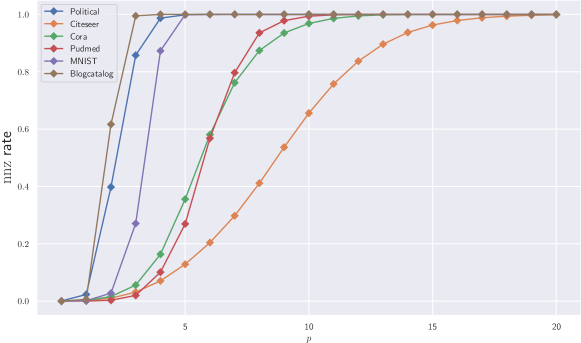
Figure 15: The $\operatorname{nnz}$ rate as a function of iteration $p$ for Approximate. The $\operatorname{nnz}$ rate, i.e., the sparsity rate of the approximated matrix, is defined as $\operatorname{nnz}{(\bm{M}_{p})}/n^{2}$ where $\operatorname{nnz}{(\bm{M}_{p})}$ is the number of nonzero entries in $\bm{M}_{p}$ after $p$ iterations. Most of these approximations become dense after 10 iterations.

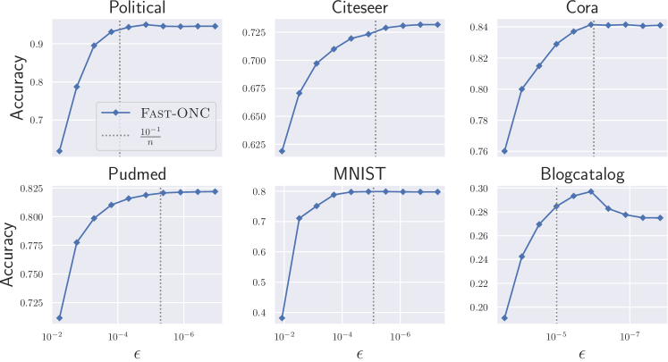
Figure 16: The overall node labeling accuracy as a function of $\epsilon$ over all six small graphs. The vertical line is when $\epsilon=\frac{10^{-1}}{n}$ corresponding to the $\epsilon$ we set in our experiments. This rough parameter estimation is good enough for most of the datasets.

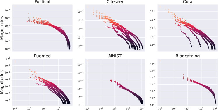
Figure 17: The power law distribution of magnitudes of $\bm{X}_{\bm{L}}$ on six small graphs. We set $\epsilon=10^{-1}/m$ and fix $\alpha=0.2$. We then randomly select 20 nodes corresponding to 20 columns of $\bm{X}_{\bm{L}}$, sort the magnitudes of $\bm{x}_{s}$, and plot them according to their rankings. These magnitudes follow the power law distribution.

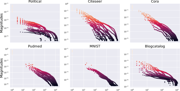
Figure 18: The power law distribution of magnitudes in $\bm{X}_{\mathcal{L}}$ on six small graphs. We set $\epsilon=10^{-1}/m$ and fix $\alpha=0.2$. We then randomly select 20 nodes corresponding to 20 columns of $\bm{X}_{\mathcal{L}}$, sort the magnitudes of $\bm{x}_{s}$, and plot them according to their rankings. These magnitudes follow the power law distribution.

References

- Adamic & Glance (2005) Adamic, L. A. and Glance, N. The political blogosphere and the 2004 us election: divided they blog. In Proceedings of the 3rd international workshop on Link discovery, pp. 36–43, 2005.
- Andersen et al. (2006) Andersen, R., Chung, F., and Lang, K. Local graph partitioning using pagerank vectors. In 2006 47th Annual IEEE Symposium on Foundations of Computer Science (FOCS’06), pp. 475–486. IEEE, 2006.
- Andersen et al. (2008) Andersen, R., Borgs, C., Chayes, J., Hopcroft, J., Jain, K., Mirrokni, V., and Teng, S. Robust pagerank and locally computable spam detection features. In Proceedings of the 4th international workshop on Adversarial information retrieval on the web, pp. 69–76, 2008.
- Anderson Jr & Morley (1985) Anderson Jr, W. N. and Morley, T. D. Eigenvalues of the laplacian of a graph. Linear and multilinear algebra, 18(2):141–145, 1985.
- Ando & Zhang (2006) Ando, R. and Zhang, T. Learning on graph with laplacian regularization. Advances in neural information processing systems, 19, 2006.
- Berkhin (2006) Berkhin, P. Bookmark-coloring algorithm for personalized pagerank computing. Internet Mathematics, 3(1):41–62, 2006.
- Blum & Chawla (2001) Blum, A. and Chawla, S. Learning from labeled and unlabeled data using graph mincuts. In Proceedings of the Eighteenth International Conference on Machine Learning, pp. 19–26, 2001.
- Blum & Mitchell (1998) Blum, A. and Mitchell, T. Combining labeled and unlabeled data with co-training. In Proceedings of the eleventh annual conference on Computational learning theory, pp. 92–100, 1998.
- Blum et al. (2004) Blum, A., Lafferty, J., Rwebangira, M. R., and Reddy, R. Semi-supervised learning using randomized mincuts. In Proceedings of the twenty-first international conference on Machine learning, pp. 13, 2004.
- Bojchevski et al. (2020) Bojchevski, A., Klicpera, J., Perozzi, B., Kapoor, A., Blais, M., Rózemberczki, B., Lukasik, M., and Günnemann, S. Scaling graph neural networks with approximate pagerank. In Proceedings of the 26th ACM SIGKDD International Conference on Knowledge Discovery & Data Mining, pp. 2464–2473, 2020.
- Cesa-Bianchi et al. (2009) Cesa-Bianchi, N., Gentile, C., and Vitale, F. Fast and optimal prediction on a labeled tree. In Annual Conference on Learning Theory, pp. 145–156. Omnipress, 2009.
- Cesa-Bianchi et al. (2013) Cesa-Bianchi, N., Gentile, C., Vitale, F., and Zappella, G. Random spanning trees and the prediction of weighted graphs. Journal of Machine Learning Research, 14(1):1251–1284, 2013.
- Chung (1997) Chung, F. R. Spectral graph theory, volume 92. American Mathematical Soc., 1997.
- DBpedia (2021) DBpedia. The DBpedia ontology. https://www.dbpedia.org/resources/ontology/, 2021. [Online; accessed 25-Jan-2023].
- El Alaoui et al. (2016) El Alaoui, A., Cheng, X., Ramdas, A., Wainwright, M. J., and Jordan, M. I. Asymptotic behavior ofell_p-based laplacian regularization in semi-supervised learning. In Conference on Learning Theory, pp. 879–906. PMLR, 2016.
- Epasto et al. (2022) Epasto, A., Mirrokni, V., Perozzi, B., Tsitsulin, A., and Zhong, P. Differentially private graph learning via sensitivity-bounded personalized pagerank. In NeurIPS 2022 Workshop: New Frontiers in Graph Learning, 2022.
- Fountoulakis & Yang (2022) Fountoulakis, K. and Yang, S. Open problem: Running time complexity of accelerated -regularized pagerank. In Conference on Learning Theory, pp. 5630–5632. PMLR, 2022.
- Fountoulakis et al. (2019) Fountoulakis, K., Roosta-Khorasani, F., Shun, J., Cheng, X., and Mahoney, M. W. Variational perspective on local graph clustering. Mathematical Programming, 174(1):553–573, 2019.
- Fu et al. (2022) Fu, G., Zhao, P., and Bian, Y. -laplacian based graph neural networks. In International Conference on Machine Learning, pp. 6878–6917. PMLR, 2022.
- Gasteiger et al. (2019) Gasteiger, J., Bojchevski, A., and Günnemann, S. Combining neural networks with personalized pagerank for classification on graphs. In International Conference on Learning Representations, 2019.
- Gentile et al. (2013) Gentile, C., Herbster, M., and Pasteris, S. Online similarity prediction of networked data from known and unknown graphs. In Conference on Learning Theory, pp. 662–695. PMLR, 2013.
- Girvan & Newman (2002) Girvan, M. and Newman, M. E. Community structure in social and biological networks. Proceedings of the national academy of sciences, 99(12):7821–7826, 2002.
- Golub & Van Loan (2013) Golub, G. H. and Van Loan, C. F. Matrix computations. JHU press, 2013.
- Gu & Han (2014) Gu, Q. and Han, J. Online spectral learning on a graph with bandit feedback. In 2014 IEEE International Conference on Data Mining, pp. 833–838. IEEE, 2014.
- Hazan et al. (2016) Hazan, E. et al. Introduction to online convex optimization. Foundations and Trends® in Optimization, 2(3-4):157–325, 2016.
- Herbster (2008) Herbster, M. Exploiting cluster-structure to predict the labeling of a graph. In International Conference on Algorithmic Learning Theory, pp. 54–69. Springer, 2008.
- Herbster & Lever (2009) Herbster, M. and Lever, G. Predicting the labelling of a graph via minimum p-seminorm interpolation. In NIPS Workshop 2010: Networks Across Disciplines: Theory and Applications, 2009.
- Herbster & Pontil (2006) Herbster, M. and Pontil, M. Prediction on a graph with a perceptron. Advances in neural information processing systems, 19, 2006.
- Herbster & Robinson (2019) Herbster, M. and Robinson, J. Online prediction of switching graph labelings with cluster specialists. Advances in Neural Information Processing Systems, 32, 2019.
- Herbster et al. (2005) Herbster, M., Pontil, M., and Wainer, L. Online learning over graphs. In Proceedings of the 22nd international conference on Machine learning, pp. 305–312, 2005.
- Herbster et al. (2008a) Herbster, M., Lever, G., and Pontil, M. Online prediction on large diameter graphs. Advances in Neural Information Processing Systems, 21, 2008a.
- Herbster et al. (2008b) Herbster, M., Pontil, M., and Galeano, S. Fast prediction on a tree. Advances in Neural Information Processing Systems, 21, 2008b.
- Herbster et al. (2015) Herbster, M., Pasteris, S., and Pontil, M. Predicting a switching sequence of graph labelings. J. Mach. Learn. Res., 16:2003–2022, 2015.
- Herbster et al. (2021) Herbster, M., Pasteris, S., Vitale, F., and Pontil, M. A gang of adversarial bandits. Advances in Neural Information Processing Systems, 34, 2021.
- Hu et al. (2020) Hu, W., Fey, M., Zitnik, M., Dong, Y., Ren, H., Liu, B., Catasta, M., and Leskovec, J. Open graph benchmark: Datasets for machine learning on graphs. Advances in neural information processing systems, 33:22118–22133, 2020.
- Jeh & Widom (2003) Jeh, G. and Widom, J. Scaling personalized web search. In Proceedings of the 12th international conference on World Wide Web, pp. 271–279, 2003.
- Johnson & Zhang (2007) Johnson, R. and Zhang, T. On the effectiveness of laplacian normalization for graph semi-supervised learning. Journal of Machine Learning Research, 8(7), 2007.
- Johnson & Zhang (2008) Johnson, R. and Zhang, T. Graph-based semi-supervised learning and spectral kernel design. IEEE Transactions on Information Theory, 54(1):275–288, 2008.
- Kipf & Welling (2017) Kipf, T. N. and Welling, M. Semi-supervised classification with graph convolutional networks. In International Conference on Learning Representations, 2017. URL https://openreview.net/forum?id=SJU4ayYgl.
- Leung et al. (2009) Leung, I. X., Hui, P., Lio, P., and Crowcroft, J. Towards real-time community detection in large networks. Physical Review E, 79(6):066107, 2009.
- Mohar (1991) Mohar, B. Eigenvalues, diameter, and mean distance in graphs. Graphs and combinatorics, 7(1):53–64, 1991.
- Namata et al. (2012) Namata, G., London, B., Getoor, L., Huang, B., and Edu, U. Query-driven active surveying for collective classification. In 10th International Workshop on Mining and Learning with Graphs, volume 8, pp. 1, 2012.
- Ng et al. (2001) Ng, A., Jordan, M., and Weiss, Y. On spectral clustering: Analysis and an algorithm. Advances in neural information processing systems, 14, 2001.
- Page et al. (1999) Page, L., Brin, S., Motwani, R., and Winograd, T. The PageRank citation ranking: Bringing order to the web. Technical Report 1999-66, Stanford InfoLab, November 1999.
- Perozzi et al. (2014) Perozzi, B., Al-Rfou, R., and Skiena, S. Deepwalk: Online learning of social representations. In Proceedings of the 20th ACM SIGKDD international conference on Knowledge discovery and data mining, pp. 701–710, 2014.
- Rakhlin & Sridharan (2015) Rakhlin, A. and Sridharan, K. Hierarchies of relaxations for online prediction problems with evolving constraints. In Conference on Learning Theory, pp. 1457–1479. PMLR, 2015.
- Rakhlin & Sridharan (2016a) Rakhlin, A. and Sridharan, K. Bistro: An efficient relaxation-based method for contextual bandits. In International Conference on Machine Learning, pp. 1977–1985. PMLR, 2016a.
- Rakhlin & Sridharan (2016b) Rakhlin, A. and Sridharan, K. A tutorial on online supervised learning with applications to node classification in social networks. arXiv preprint arXiv:1608.09014, 2016b.