Proof.

Moravian University
Bethlehem, PA

On the $n$-attack Roman Dominating Number of a Graph

Garrison Koch

Advisor: Dr. Nathan Shank
Liaison: Dr. Ben Coleman

2023

Copyright 2023 Garrison L. Koch

Abstract

The Roman Dominating number is a widely studied variant of the dominating number on graphs. Given a graph $G=(V,E)$, the dominating number of a graph is the minimum size of a vertex set, $V^{\prime}\subseteq V$, so that every vertex in the graph is either in $V^{\prime}$ or is adjacent to a vertex in $V^{\prime}$. A Roman Dominating function of $G$ is defined as $f:V\rightarrow\{0,1,2\}$ such that every vertex with a label of 0 in $G$ is adjacent to a vertex with a label of 2. The Roman Dominating number of a graph is the minimum total weight over all possible Roman Dominating functions. In this paper, we analyze a new variant: $n$-attack Roman Domination, particularly focusing on 2-attack Roman Domination $(n=2)$. An $n$-attack Roman Dominating function of $G$ is defined similarly to the Roman Dominating function with the additional condition that, for any $j\leq n$, any subset $S$ of $j$ vertices all with label 0 must have at least $j$ vertices with label 2 in the open neighborhood of $S$. The $n$-attack Roman Dominating number is the minimum total weight over all possible $n$-attack Roman Dominating functions. We introduce properties as well as an algorithm to find the 2-attack Roman Domination number. We also consider how to place dominating vertices if you are only allowed a finite number of them through the help of a python program. Finally, we discuss the 2-attack Roman Dominating number of infinite regular graphs that tile the plane. We conclude with open questions and possible ways to extend these results to the general $n$-attack case.

I would like to thank my wonderful advisor Dr. Shank who spent countless hours, planned and impromptu, working with me to ensure this project and paper could be done at our fullest capability. Without his guidance and willingness to push me, this project would not be what it is. Thank you to my liaison and honors panel for their advice and diligent feedback. Lastly, thank you to my mother, Dr. Pam Koch, for providing support throughout, as well as an occasional ear to vent to.

Contents

1. 1 $n$-Attack Roman Domination
   1. 1.1 Background and Motivation
   2. 1.2 Introduction
      1. 1.2.1 Public and Private Neighbors
   3. 1.3 Complete Graphs and Star Graphs
2. 2 Optimality
   1. 2.1 Notation
   2. 2.2 What Graphs are Optimal?
   3. 2.3 Finding the Minimum labeling
3. 3 Density and Infinite Graphs
   1. 3.1 Density
   2. 3.2 Infinite Graphs
   3. 3.3 Graphs that Tile the Plane
4. 4 Properties, Connections, and Applications
   1. 4.1 Exterior Private Neighbors and Minimum Weight Labelings
   2. 4.2 Connections To Other Results
      1. 4.2.1 Maximum Degree Bound
      2. 4.2.2 Menger’s Theorem Connection
   3. 4.3 Applications
      1. 4.3.1 Using The Programs
5. 5 Conclusion
   1. 5.1 Future Work

Chapter 1 $n$-Attack Roman Domination

1.1. Background and Motivation

Roman Domination ($RD$) is a variation on the common graph property - dominating number. Recall that given a finite simple graph $G:=(V,E)$ where $V$ is a vertex set and $E$ is a set of edges between these vertices, a set $V^{\prime}\subseteq V$ is a dominating set if every vertex $v\in V$ is in $V^{\prime}$ or adjacent to a vertex in $V^{\prime}$. The minimum size of all the dominating sets is called the dominating number of the graph and is denoted $\gamma(G)$. Any dominating set, $V^{\prime}$ with $|V^{\prime}|=\gamma(G)$ is called a minimum dominating set. Thus $\gamma(G)=\min\{|V^{\prime}|:V^{\prime}\text{ is a dominating set for }G\}$. For other common graph theory notation and terminology used throughout, we refer the reader to [2].

The Roman Domination number of a graph acts similarly to a dominating number, in that the goal is to find the least domination required for every vertex on the graph to be dominated. Roman Domination is said to be derived from the Emperor Constantine who had to decide where to station his four army units to protect eight regions [4]. In this context, Roman Domination places 0, 1, or 2 armies at each region in such a way so that any region with 0 armies must be adjacent to a region with 2 armies, thus providing protection to the abandoned region. The minimum number of armies to protect the entire country is the Roman Dominating number, denoted $\gamma_{R}(G)$. This will be formally defined in Section 1.2.

Xu in [6] provided multiple bounds for the Roman Dominating number of graphs. The most simple bound she discusses is that $\gamma(G)\leq\gamma_{R}(G)\leq 2\gamma(G)$ as letting all of the vertices in the minimum dominating set of $G$ have a label of 2 will be a valid labeling for the Roman Dominating function. This bound does not hold for our new 2-attack Roman Dominating number, as we will soon see. Xu continues on to find the general Roman Dominating number for simple graphs like paths, trees, and cycles, which we will explore for the 2-attack case, as well.

Roman Domination has since been extended to Double and even Triple Roman Domination. In 2016, Beeler et. al. published a thorough paper on Double Roman Domination, properties of the function and a comparison to Roman Domination [1]. Double Roman Domination allows for the use of 3, 2, 1, or 0 as vertex labels. In [1], they prove that you never need to label a vertex 1 in the minimum weight Double Roman Domination labeling. We see an analogous property occur in 2-attack, but only in some special cases and for infinite graphs.

Roman Domination is a variant on dominating number as it increases how dominated vertices are. Double and Triple Roman Domination continue with this idea of finding ways to increase the fortification on vertices (ports). Continuing with the army semantic theme, we have created $n$-attack Roman Domination ($nRD$) under the idea of how many of our vertices (ports) are being attacked. The $n$ in this case is the number of enemy armies which are attacking. Thus, 1-attack Roman Domination means our enemy has one army and will attack in one spot, so the original Roman Domination would suffice. If however, we consider 2-attack Roman Domination, we must fortify against two armies simultaneously attacking. So a structure like the one in Figure 1.1 would be defended in a 1-attack Roman Domination (i.e. satisfy a Roman Domination labeling), but not a 2-attack Roman Domination. If both unfortified ports (the vertices with value 0) were attacked, the other port cannot defend both while still maintaining a presence at its own port.

Figure 1.1. Valid Roman Domination labeling but not valid for $2RD$

Note, however, if we change one of the labels from 0 to 1, then Figure 1.1 would be defended in a 2-attack Roman Domination.

Optimization problems like these have many more practical applications than army semantics, and thus are a very pragmatic area to study. In this paper, we will introduce some simple finite and infinite graph classes and examine their $2RD$ number or density. We will also unpack several properties of our dominating variant as well as provide an algorithm to find the $2RD$ number for any finite graph.

1.2. Introduction

Roman Domination was introduced by Cockayne et al. [4] in 2004. Let $G=(V,E)$ be a simple graph. Cockayne defines a Roman Dominating function on $G$ as $f_{G}:V\rightarrow\{0,1,2\}$ such that every vertex with a label of 0 in $G$ is adjacent to a vertex with a label of 2. The weight of a Roman Dominating function, $f_{G}$, is $\displaystyle w(f_{G})=\sum_{v\in V(G)}f_{G}(v)$. When the underlying graph $G$ is well understood, we will write $f=f_{G}$ and $w(f)=w(f_{G})$. The Roman Domination number of a graph $G$, denoted $\gamma_{R}(G)$, is the minimum weight of all possible Roman Dominating functions on $G$. If $w(f_{G})=\gamma_{R}(G)$ we will say that $f$ is a minimum weight Roman Dominating function. Xu in [6] introduced bounds for the Roman Dominating function using dominating function as well as the maximum and minimum degree in the graph. More recently, Shao et al. in [8] considered how taking cartesian products of known graph classes affects the $RD$ number of the resulting graphs.

Beeler et al. in [1] considered an expansion on Roman Domination, $n$-Roman Domination. In the case when $n=2$, Beeler et al. analyzed Double Roman Domination defined as a function $f_{G}:V\rightarrow\{0,1,2,3\}$ on graph $H=(V,E)$ such that if $f(v)=0$, then $v$ must be adjacent to at least two vertices with label 2 or one vertex with label 3.

Let $N(v)$ denote the open neighborhood of the vertex $v$, i.e the vertices in which $v$ is adjacent to. The open neighborhood of a set of vertices $S\subset V(G)$, is represented as $\displaystyle N(S)=\left(\bigcup_{v\in S}N(v)\right)\backslash S$, i.e. $N(S)$ consists of all vertices not in $S$, but adjacent to a vertex in $S$.

In this paper, we define a new measure of domination called the $n$-attack Roman Domination.

Definition 1.1.

Let $G=(V,E)$ be a simple graph. A $n$-attack Roman Domination function of $G$ is defined as $f_{G}:V\rightarrow\{0,1,2\}$ such that any vertex $v$ where $f_{G}(v)=0$ is adjacent to a vertex $u$ where $f_{G}(u)=2$. Additionally, for any $j\leq n$, any subset $S$ of $j$ vertices all with label 0, must have at least $j$ vertices with label 2 in $N(S)$.

Similar to $RD$, we let the weight of an $n$-attack Roman Dominating function, $f_{G}$, be $\displaystyle w(f_{G})=\sum_{v\in V(G)}f_{G}(v)$. When the underlying graph $G$ is well understood, we will write $f=f_{G}$ and $w(f)=w(f_{G})$. The $n$-attack Roman Domination number of a graph $G$, denoted $\gamma_{nR}(G)$, is the minimum weight of all possible $n$-attack Roman Dominating functions on $G$. If $w(f_{G})=\gamma_{nR}(G)$ we will say that $f$ is a minimum weight $n$-attack Roman Dominating function.

As defined, 1-attack Roman Domination is equivalent to the original Roman Domination. In this paper, we will primarily focus on 2-attack Roman Domination, but will make generalizations to $n$-attack Roman Domination when relevant.

1.2.1. Public and Private Neighbors

Given a function $f$ on $G$, we will henceforth denote the set of vertices in a graph $G$ with label 0 as $V_{0}(f)$, the set of vertices in $G$ with label 1 as $V_{1}(f)$, and the set of vertices in $G$ with label 2 as $V_{2}(f)$. So

$$f(v)=\begin{cases}0,\text{ if }v\in V_{0}(f)\\ 1,\text{ if }v\in V_{1}(f)\\ 2,\text{ if }v\in V_{2}(f).\\ \end{cases}$$

We understand the above idea of $f$ is somewhat circular. However, it illustrates the point that we will sometimes define $f$ directly or we can define $f$ based on a partitioning of the vertex set. This notion of partitioning the vertex set by their labels can be extended so that $v\in V_{i}(f)$ if and only if $f(v)=i$. We will often use $V_{0},V_{1},$ and $V_{2}$ when the labeling $f$ is well understood or if we are defining a labeling in terms of a partition of the vertices.

In addition, we will use similar terminology as was done with dominating number and dominating sets. For example, if $f$ is a $n$-attack Roman Dominating function of $G$, then the vertices in $V_{2}(f)$ $nR$ Dominate the vertices in $V_{0}(f)$. Vertices in $V_{1}(f)$ are still considered part of the dominating set, but as discussed, these vertices cannot dominate any vertex other than itself.

Note that $V_{0}\cup V_{1}\cup V_{2}=V(G)$. We say a vertex $v\in V_{2}$ has a private neighbor $u$ with respect to the set $V_{2}$ if $uv\in E(G)$ but $u$ is not adjacent to any other vertex in $V_{2}$. While these neighbors could have any label, in this paper when we discuss private neighbors of $V_{2}$ we are specifically referring to vertices with label 0. We will examine the implications of these private neighbors on the $n$-attack Roman Domination Number of graphs. Private neighbors have been extensively studied and are well understood and their importance is extremely valuable when studying domination in graphs. Haynes [5] defines the private neighbor of a vertex $v$ relative to a set $S$ of vertices as $pn(v,S)=\{u\in V:N(u)\cap S=\{v\}\}$. For example, $u$ is a private neighbor of $v$ with respect to the set $S$ if $u$ is adjacent to $v$ and $u$ is not adjacent to any other vertex in $S$. Haynes goes on to define exterior private neighbors as $epn(v,S)=pn(v,S)\cap(V-S)$. That is to say, if $u$ is a private neighbor of $v$ with respect to $S$, $u$ is also an exterior private neighbor if $u\notin S$.

We now define the public neighborhood of a set $S\subseteq V$ as $\overline{p}n(S)=\{u\in V:|N(u)\cap S|\geq 2\}$. For example, $u$ is in the public neighborhood of the set of vertices $S$ if $u$ is adjacent to at least two vertices in $S$. We define the exterior public neighborhood of a set $S$ as $\overline{ep}n(S)=\overline{p}n(v,S)\cap(V-S)$.

We can extend the private neighbor definition to be defined solely on a set, analogous to the public neighborhood definition we have just outlined.

Definition 1.2.

A vertex $v$ is an exterior private neighbor of a set $S$ if $v\notin S$ and $v$ is adjacent to exactly one vertex in $S$. A vertex $u$ is an exterior public neighbor of a set $S$ if $u\notin S$ and $u$ is adjacent to more than one vertex in $S$.

Exterior public and exterior private neighborhoods will be necessary as we will distinguish between vertices in $V_{0}$ which are (exterior) private neighbors of $V_{2}$ and vertices in $V_{0}$ that are (exterior) public neighbors of $V_{2}$.

1.3. Complete Graphs and Star Graphs

When one begins studying the dominating function, complete graphs and star graphs are often used to demonstrate the efficiency of small dominating sets. While those graph classes also have small Roman Dominating numbers, that is not the case for $2RD$. For a complete graph of order $n$, denoted $K_{n}$, note that $\gamma(K_{n})=1$ and $\gamma_{R}(K_{n})=2$. Consider a $K_{3}$ and note that the minimum $2RD$ labeling is either a 0,1,2 or a 1,1,1 labeling of the three vertices. If we consider a $K_{4}$, there are more minimum $2RD$ labelings (0,2,0,2 or 1,1,1,1 for instance), all of which have a weight of 4. Notice that for any $K_{n}$ where $n\geq 4$, we have $\gamma_{2R}(K_{n})=4$, as two vertices with label 2 are sufficient to $2R$ Dominate the rest of the vertices. Note that if we only have one vertex with label 2, we can only have one vertex of label 0, and the rest of the vertices will have a label of 1. With two vertices of label 2, they can sufficiently $2R$ Dominate the rest of the vertices in the graph. A $2RD$ labeling of $K_{6}$ is demonstrated in figure 1.2 to illustrate this point.

Figure 1.2. Minimum Weight $2RD$ labeling of $K_{6}$

This proves the following simple results:

Theorem 1.1.

Let $K_{n}$ be a complete graph on $n$ vertices, then

$$\gamma_{2R}(K_{n})=\begin{cases}n,\text{ if }n<4\\ 4,\text{ if }n\geq 4.\\ \end{cases}$$

Moving on to star graphs, we begin by noting that once again $\gamma(K_{1,n})=1$ and $\gamma_{R}(K_{1,n})=2$. If we wanted to find a minimum weight $2RD$ labeling, we can begin by letting the center vertex have a label of 2. However, we will quickly note that while we can let one leaf vertex have a label of 0, all the other leaves must have a label of 1. With some exploration, we can easily show the following:

Theorem 1.2.

Let $K_{1,n}$ be a star graph on $n+1$ vertices, then

$$\gamma_{2R}(K_{1,n})=n+1.$$

An example $K_{1,4}$ is shown in Figure 1.3 to illustrate the three different dominating functions.

(a) Dominating

(b) Roman Dominating

(c) 2-attack $RD$

Figure 1.3. Different dominating functions on $K_{1,4}$

As exemplified by the example above, it is not uncommon for a graph’s $2RD$ number to be equal to the order of the graph. In the next chapter, we will introduce the idea of optimality to articulate this point.

Chapter 2 Optimality

For most non-trivial graphs, the dominating and Roman Dominating numbers are less than the order of the graph. For example, simple reasoning leads us to the following conclusions. The size of $G$ is at least one if and only if $\gamma(G)<|V(G)|$. Similarly, $\Delta(G)\geq 2$ if and only if $\gamma_{R}(G)<|V(G)|$. Note that $\Delta(G)$ is the maximum degree of $G$. This is not so simple for the 2-attack Roman Dominating number as we saw in Section 1.3. We noted that there is a simple upper bound for $2RD$, which is formally stated below.

Proposition 2.1.

For any graph $G$, $\gamma_{nR}(G)\leq|V(G)|$.

We can let $V_{1}=V(G)$, thus $w(f_{G})=|V(G)|$. This will always be a valid $nRD$ labeling. ∎ Now, we want to differentiate between graphs for which $\gamma_{nR}(G)<|V(G)|$ and $\gamma_{nR}(G)=|V(G)|$. So, we define optimality and optimal number below.

Definition 2.1.

For a finite graph $G$, if $\gamma_{nR}(G)=|V(G)|$, then $G$ is called sub-optimal. If $\gamma_{nR}(G)<|V(G)|$, then $G$ is called optimal. If a graph is optimal, the difference, $|V(G)|-\gamma_{nR}(G)$, is called the optimal number.

For the original domination function, the star graph is dominated by 1 single vertex who has the ability to dominate all the adjacent vertices. As seen in Section 1.3, the same can not be said for $2RD$. There is, however, a similar graph class for $2RD$ that, like the star, can be 2-attack Roman Dominated by just two vertices: $K_{2,n}$ as shown in figure 2.1. Note, like the star, $n$ can be large and the labeling is still valid.

Figure 2.1. $K_{2,n}$ with the minimum weight $2RD$ labeling

Note that this graph resembles a star graph, but instead we have two vertices that dominate the rest of the graph instead of only one.

2.1. Notation

In order to explore the conditions a graph needs to be optimal as well as how to find the graphs optimal number, we must introduce some notation. As we have mentioned on a few occasions, we are often interested in the minimum weight $2RD$ labeling on a graph. While some graphs, like the one in Figure 2.1 have a unique minimum labeling, many graphs (see Figure 2.2) have several.

Figure 2.2. A graph with multiple minimum labelings (two shown here)

So, we introduce a way to denote all of the minimum labelings of a particular graph.

Definition 2.2.

Let $\Gamma_{2R}(G)$ be the set of all valid minimum labelings on $G$:

$$\Gamma_{2R}(G)=\{f_{G}:w(f_{G})=\gamma_{2R}(G)\}.$$

Notice that both labelings in Figure 2.2 are minimum and thus would be elements of $\Gamma_{2R}(G)$. Throughout we will assume that $\ell_{G}:V(G)\rightarrow\{0,1,2\}$ will denote a labeling in $\Gamma_{2R}(G)$. So $w(\ell_{G})=\gamma_{2R}(G)$. When discussing labels of sequential vertices in a graph, we will use dashes to delineate the subpath of vertices we wish to highlight. For instance, the graph in Figure 2.3 has a subgraph labeled 0-2-1 and a subgraph labeled 1-1-2-0, but they are not disjoint subpaths.

Figure 2.3. A graph with labeling 0-2-1-1

Lastly, recall Definition 1.2. We noted following that definition that exterior public and exterior private neighborhoods will be useful when discussing how $V_{2}(f)$ interacts with $V_{0}(f)$.

Definition 2.3.

Given a graph $G$ and labeling $f_{G}$, if a vertex $v\in V_{0}(f_{G})$ is adjacent to exactly one vertex in $V_{2}(f_{G})$, then we say $v\in epn(V_{2}(f_{G}))$. If a vertex $u\in V_{0}(f_{G})$ is adjacent to more than one vertex in $V_{2}(f_{G})$, then we say $u\in\overline{ep}n(V_{2}(f_{G}))$.

For emphasis, we are only referring to vertices with label 0 for these neighborhoods. A vertex with label 1 will never be considered in the exterior public or private neighborhood of $V_{2}$. Since neighborhoods are sets of vertices, the cardinality of the set (i.e $|epn(V_{2}(f_{G}))|$) refers to the number of vertices in the exterior private neighborhood.

2.2. What Graphs are Optimal?

In this section, we will discuss what properties a graph must have to be optimal, and how to find the 2-attack Roman Dominating number of any graph. The following proposition is intuitive but important for the subsequent theorem.

Proposition 2.2.

A finite graph $G$ is optimal if and only if there is a $2RD$ labeling $\ell\in\Gamma_{2R}(G)$ so that $|V_{2}(\ell)|<|V_{0}(\ell)|$.

Note that if there exists a $2RD$ labeling $\ell\in\Gamma_{2R}(G)$ with $|V_{2}(\ell)|<|V_{0}(\ell)|$ then $|V_{0}(\ell)|-|V_{2}(\ell)|=|V(G)|-\gamma_{2R}(G)$. Thus any other $2RD$ labeling $\ell^{\prime}\in\Gamma_{2R}(G)$ will have $|V_{2}(\ell^{\prime})|<|V_{0}(\ell^{\prime})|$. We use this idea to help prove the following theorem.

Theorem 2.3.

A graph $G$ is optimal if and only if for every labeling $\ell_{G}\in\Gamma_{2R}(G)$, there exists a $P_{5}$ subgraph in $G$ labeled 0-2-0-2-0 under $\ell_{G}$.

Part 1: ($\Leftarrow$) If $G$ has a $P_{5}$ subgraph with such a labeling, $G$ is optimal.

Assume $G$ has a $P_{5}$ subgraph, $abcde$, which is labeleled 0-2-0-2-0 under $\ell$. Let $f(a)=f(c)=f(e)=0$. Let $f(b)=f(d)=2$. Let $f(v)=1$ for all other $v\in V(G)$. This is a valid $2RD$ labeling, where $w(\ell)\leq w(f_{G})<|V(G)|$. Since the weight of any valid $2RD$ labeling is greater than or equal to $\gamma_{2R}(G)$, it follows that $\gamma_{2R}(G)<|V(G)|$ and thus $G$ is optimal.

Part 2: ($\Rightarrow$) If $G$ is optimal, $G$ has a $P_{5}$ subgraph labeled 0-2-0-2-0 in $\ell$.

Let $\ell\in\Gamma_{2R}(G)$. By Proposition 2.2, we know $|V_{0}|>|V_{2}|$. Since $V_{0}$ is non-empty, then $V_{2}$ must also be non-empty for the labeling to be valid. If every $v\in V_{2}$ is only adjacent to one vertex with label 0, then $|V_{0}|=|V_{2}|$ which is a contradiction. So, there must be a $b\in V_{2}$ where $b$ is adjacent to at least two vertices with label 0 (call them $a$ and $c$). Since $\ell$ is a valid labeling, either $a$ or $c$ ($wlog$ assume it is $c$) must be adjacent to another vertex with label 2 (call this vertex $d$). If $d$ is adjacent to another 0, we have found a $P_{5}$ with a 0-2-0-2-0 labeling and we are done. If not, relabel $d$ and $c$ to both have a label of 1 (as shown in Figure 2.4). Call this labeling $\ell^{1}$. Note, $w(\ell)=w(\ell^{1})$ so $\ell^{1}\in\Gamma_{2R}(G)$, which tells us that $|V_{0}(\ell^{1})|=|V_{0}(\ell)|-1$ and $|V_{2}(\ell^{1})|=|V_{2}(\ell)|-1$ and so $|V_{0}(\ell^{1})|-|V_{2}(\ell^{1})|=|V_{0}(\ell)|-|V_{2}(\ell)|>0$.

Note that $\ell$ and $\ell^{1}$ are equal on all vertices in $V_{0}(\ell^{1})\cup V_{2}(\ell^{1})$. So, if there is a 0-2-0-2-0 $P_{5}$ subgraph in $G$ under $\ell^{1}$, then the same $P_{5}$ subgraph and labeling will exists under $\ell$. Find another vertex, $b^{1}\in V_{2}(\ell^{1})$ that has two adjacent vertices with label 0 (call them $a^{1}$ and $c^{1}$) and repeat this process. If we reach a point where every vertex in $V_{2}(\ell^{n})$ is adjacent to at most one vertex with label 0, as stated previously there is no way to have $|V_{0}(\ell)|>|V_{2}(\ell)|$, which violates our assumption that $G$ is optimal.

Figure 2.4. Turning a 2-0 pair into a 1-1 pair

Theorem 2.3 is incredibly useful, as it is a quick way not only to tell whether a graph is optimal or not, but gives us a start for what an optimal $2RD$ labeling would look like. In the next section, we will consider how to find the minimum $2RD$ labeling of any graph.

2.3. Finding the Minimum labeling

In order to reach a discussion on finding a minimum $2RD$ labeling of a graph $G$, $\ell_{G}$, we must first introduce the concept of end-coupled center disjoint $P_{5}$ subgraphs. First, we will formally define end-coupled center disjoint ($eccd$) $P_{5}$ subgraphs, and then look at an example to understand each condition.

Definition 2.4.

Let $S$ be a set of $P_{5}$ subgraphs of $G$. For $S$ to be a valid set of end-coupled center disjoint $P_{5}$ subgraphs:

• Let $v_{a}-v_{b}-v_{c}-v_{d}-v_{e}$ be some $P_{5}$ in $S$. If $v_{a}$ or $v_{b}$ is a vertex in some other $P^{\prime}_{5}$ in $S$, then $v_{a}v_{b}\in E(P^{\prime}_{5})$, where $v_{a}$ is a leaf. Analogously, if $v_{e}$ or $v_{d}$ is a vertex in some other $P^{\prime\prime}_{5}$ in $S$, then $v_{e}v_{d}\in E(P^{\prime\prime}_{5})$, where $v_{e}$ is a leaf.

• Let $v_{a}-v_{b}-v_{c}-v_{d}-v_{e}$ be some $P_{5}$ in $S$. No other $P_{5}$ in $S$ may use the vertex $v_{c}$.

So, if every $eccd$ in $S$ is completely disjoint, $S$ is a valid set of $eccd$’s. If there is overlap (vertices appear in multiple subgraphs in $S$), then the overlap must be done “correctly” in the manner described.

Figure 2.5. A graph with several possible $eccd$ sets

Consider the graph in Figure 2.5 as we walk through various valid and invalid $eccd$ sets. Most obviously, $v_{1}-v_{2}-v_{3}-v_{4}-v_{5}$ and $v_{6}-v_{7}-v_{8}-v_{9}-v_{10}$ would make up a valid set of $eccd$’s as they are completely disjoint. However, $v_{1}-v_{2}-v_{8}-v_{4}-v_{5}$ and $v_{6}-v_{7}-v_{8}-v_{9}-v_{10}$ would not be a valid $eccd$ set as it violates the center disjoint criteria. Additionally, we notice that $v_{1}-v_{2}-v_{3}-v_{4}-v_{5}$ and $v_{6}-v_{7}-v_{8}-v_{4}-v_{5}$ do make a valid set of $eccd$’s as they overlap on $v_{4}-v_{5}$, but that end coupling is held through both subgraphs. Alternatively, the subgraphs $v_{1}-v_{2}-v_{3}-v_{4}-v_{5}$ and $v_{10}-v_{9}-v_{8}-v_{5}-v_{4}$ would not be a valid $eccd$ set as $v_{4}-v_{5}$ are coupled in both, but appear in the wrong order ($v_{5}$ is a leaf in one subgraph and $v_{4}$ is a leaf in the other subgraph). So in summary, Definition 2.4 is saying that a set of $P_{5}$ subgraphs form a set, $S$, of end-coupled center disjoint subgraphs if no two subgraphs in $S$ have the same center and if two $P_{5}$’s in $S$ intersect they can only intersect on the end edges and the intersection must be in the correct order.

For the graph in Figure 2.5, there are several valid sets of $eccd$ subgraphs, the largest sets having size 2. With some exhaustion we can convince ourselves that no set of 3 $eccd$’s exists for this graph, though it is not immediately apparent. This is one reason why having a computer program to find this answer more efficiently is useful (discussed more in Section 4.3).

Before implementing the use of $eccd$’s in a graph, we must first consider the following proposition and lemma on how the label 0 and 2 vertex sets of a graph interact.

Proposition 2.4.

Given a finite graph $G$ with $\ell_{G}\in\Gamma_{2R}(G)$, every vertex in $V_{2}$ is adjacent to at least one vertex in $V_{0}$.

Consider a finite graph $G$ with a minimum $2RD$ labeling $\ell_{G}$. Assume, by way of contradiction, there exists a vertex $v\in V_{2}$ that does not have any neighbors in $V_{0}$. We can relabel $v$ to be in $V_{1}$, which produces a valid $2RD$ labeling with a smaller weight than $\ell_{G}$. Thus $\ell_{G}$ was not of minimum weight, which is a contradiction. This proposition informs the following lemma.

Lemma 2.5.

Given a finite graph $G$ with minimum $2RD$ labeling $\ell_{G}\in\Gamma_{2R}(G)$, there exists a spanning subgraph $G^{\prime}$ with induced labeling $\ell_{G^{\prime}}=\ell_{G}$, where every $v\in V_{2}$ has an $epn$ in $G^{\prime}$. In other words, there exists a bijection between $V_{2}$ and some $V^{\prime}_{0}\subseteq V_{0}$.

Consider a finite graph $G$ with $\ell_{G}\in\Gamma_{2R}(G)$. Consider a matching, $M$, in $G$ so that every vertex in $V_{2}$ which has an $epn$ is matched with its $epn$. Now, label all the remaining vertices in $V_{2}$ as $t_{1},t_{2},\ldots,t_{k}$. Note that each $t_{i}$ has no $epn$ but must be adjacent to at least one vertex in $V_{0}$ by Proposition 2.4. Now, pick a $v_{1}\in V_{0}$ adjacent to $t_{1}$ and remove the edges from $v_{1}$ to any vertex in $V_{2}\backslash t_{1}$. Call this spanning subgraph $G^{1}$. Notice in $G^{1}$, $v_{1}$ is the $epn$ of $t_{1}$. The induced labeling, $\ell_{G^{1}}$ on $G^{1}$ is valid by construction and has the same weight as $\ell_{G}$ thus is still minimum. Note Proposition 2.4 still holds for $G^{1}$. Now, pick a $v_{2}\in V_{0}$ adjacent to $t_{2}$ in $G^{1}$ and remove the edges from $v_{2}$ to any vertex in $V_{2}\backslash t_{2}$. Call this spanning subgraph $G^{2}$. Notice that in $G^{2}$, the vertex $v_{2}$ is an $epn$ of $t_{2}$. Repeat this process for every vertex $t_{i}$ for $1\leq i\leq k$. We will end with a subgraph $G^{k}$ with a minimum $2RD$ labeling $\ell_{G^{k}}$ where every vertex in $V_{2}$ has an $epn$ in $G^{k}$.

Now that we have a more precise understanding of how the label sets 0 and 2 interact in a minimum labeling, we can use the number of $eccd$’s subgraphs in a graph to indicate the graph’s optimal number. While it may seem that the two properties are completely unrelated, we discuss a similar theorem in Section 4.2.2. For notation, if $S$ is a set of end-coupled center disjoint $P_{5}$ subgraphs of $G$, we will say $S$ is an $ECCD{(G)}$. Given a graph $G$, let $\mathbb{S}=\{S:S\text{ is an }ECCD{(G)}\}$. So $\mathbb{S}$ is the set of all subsets of end-coupled center disjoint $P_{5}$ subgraphs of $G$.

Theorem 2.6.

The optimal number (recall Definition 2.1) of a finite graph $G$ is equal to the maximum number of distinct end-coupled center disjoint $P_{5}$ subgraphs in $G$:

$$|V(G)|-\gamma_{2R}(G)=\max\{|S|:S\in\mathbb{S}\}.$$

Before we prove this theorem, it is helpful to note that a labeling constructed from a set of $eccd$ $P_{5}$ subgraphs is valid.

Lemma 2.7.

Given a graph $G$ and a set of $S$ of $eccd$ subgraphs in $G$. Define a labeling $e_{G}$ where we label every $eccd$ subgraph in $S$ $0-2-0-2-0$ (some vertices may receive a label more than once, but each time it will be the same value by construction). Give every vertex in $G\backslash S$ a label of 1. $e_{G}$ is a valid labeling

Let $e_{G}$ be a labeling on $G$ as described. We can break down the definition of $2RD$ into two components. Every 0 must be adjacent to a 2. Every pair of two 0’s must be adjacent to at least two 2’s. So, if $e_{G}$ was to be an invalid labeling, it would fail one of these criteria. Notice that if you label $eccd$’s in the manner described, and those are the only vertices in $V_{0}(e)$, every 0 will be adjacent to at least one 2. Now, assume for the sake of contradiction, there are two vertices $a,b\in V_{0}(e)$ which are both only adjacent to $c\in V_{2}(e)$. Neither $a$ or $b$ can be a center vertex of an $eccd$ (or else they would be adjacent to two 2’s on their own), which implies that $c$ was coupled with two vertices, which contradicts how $eccd$’s are picked.

Now, to prove Theorem 2.6, it is equivalent to show that the maximum number of distinct $eccd$ $P_{5}$ subgraphs is equal to the difference $|V_{0}|-|V_{2}|$ of $\ell_{G}$. For ease of notation, let $\max\{|S|:S\in\mathbb{S}\}=\mathbf{E}(G)$. (Proof of Theorem 2.6)

Given a finite graph $G$ with labeling $\ell_{G}$, construct a spanning subgraph $G^{\prime}$ with $\ell_{G^{\prime}}=\ell_{G}$ for all $v\in V(G^{\prime})$, such that every $v\in V_{2}(\ell_{G^{\prime}})$ has an $epn$. Let $V^{\prime}_{0}(\ell_{G^{\prime}})$ denote the set of $epn$’s of $V_{2}(\ell_{G^{\prime}})$ noting that $|V_{0}^{\prime}(\ell_{G^{\prime}})|=|V_{2}(\ell_{G^{\prime}})|$. This construction is possible by Lemma 2.5. Now let $V^{\prime\prime}_{0}(\ell_{G^{\prime}})=V_{0}(\ell_{G^{\prime}})\backslash V^{\prime}_{0}(\ell_{G^{\prime}})$. By construction, every vertex in $V^{\prime\prime}_{0}(\ell_{G^{\prime}})$ is a public neighbor of $V_{2}(\ell_{G^{\prime}})$. Recall that the optimal number of $G$ is $|V_{0}(\ell_{G})|-|V_{2}(\ell_{G})|$ and $|V_{0}(\ell_{G})|-|V_{2}(\ell_{G})|=|V^{\prime\prime}_{0}(\ell_{G^{\prime}})|+|V^{\prime}_{0}(\ell_{G^{\prime}})|-|V_{2}(\ell_{G^{\prime}})|$. Therefore, the optimal number of $G$ is $|V^{\prime\prime}_{0}(\ell_{G^{\prime}})|$.

So, we now will show that $|V^{\prime\prime}_{0}(\ell_{G^{\prime}})|$ is equal to the number of $eccd$ $P_{5}$ subgraphs in $G$. First, note we can take the $\max\{|S|:S\in\mathbb{S}\}$ and use said $S$ to create a labeling $e_{G^{\prime}}$ in the manner described in Lemma 2.7. We know this labeling is valid, and can deduce that $|V(G^{\prime})|-w(e_{G^{\prime}})=\mathbf{E}(G)$. Therefore if $\mathbf{E}(G)$ was greater than $V^{\prime\prime}_{0}(\ell_{G^{\prime}})$, then $w(e_{G^{\prime}})<w(\ell_{G^{\prime}})$, which is a contradiction as $\ell_{G^{\prime}}$ is assumed to be minimum. This implies $|V^{\prime\prime}_{0}(\ell_{G^{\prime}})|\geq\mathbf{E}(G)$.

Note that every vertex in $V^{\prime\prime}_{0}(\ell_{G^{\prime}})$ is the center of a $P_{5}$ since each vertex in $V^{\prime\prime}_{0}(\ell_{G^{\prime}})$ must be adjacent to at least two vertices in $V_{2}(\ell_{G^{\prime}})$ and each vertex in $V_{2}(\ell_{G^{\prime}})$ is coupled with a vertex in $V^{\prime}_{0}(\ell_{G^{\prime}})$. Therefore, each of these $P_{5}$ are center disjoint. Also, each of these $P_{5}$’s is end-coupled by construction. This implies $|V^{\prime\prime}_{0}(\ell_{G^{\prime}})|\leq\mathbf{E}(G)$. Therefore, $|V^{\prime\prime}_{0}(\ell_{G^{\prime}})|=\mathbf{E}(G)$.

We have shown that finding the maximum number of $eccd$ subgraphs tells us the optimal number of a graph, but in fact, it does more than that. Lemma 2.7 tells us that we can construct a valid labeling where every $eccd$ subgraph is labeled $0-2-0-2-0$ (with every other vertex receiving a label of 1). Not only will a labeling of this manner be valid, but it will also be minimal.

Corollary 2.8.

The maximum set of $eccd$ $P_{5}$ subgraphs of a graph $G$ gives us a minimum weight $2RD$ labeling of $G$, $\ell^{*}_{G}$, where $w(\ell^{*}_{G})=\gamma_{2R}(G)$.

Given a graph $G$ we can use lemma 2.7 to create a labeling $\ell^{*}_{G}$. Let $\ell^{*}_{G}$ be a labeling where we take the largest set $S$ of $eccd$’s in $G$ and label each $0-2-0-2-0$ with every other vertex receiving a label of 1. Lemma 2.7 ensures this labeling is valid. As discussed in the proof of theorem 2.6, we know $|V(\ell^{*}_{G})|-w(\ell^{*}_{G})=|S|$. (Recall $|V(\ell^{*}_{G})|-w(\ell^{*}_{G})=|V_{0}(\ell^{*}_{G})|-|V_{2}(\ell^{*}_{G})|$ and every $eccd$ adds one to the latter difference.) Since $S$ is the maximum set of $eccd$’s in $G$, it follows that

$$|V(G)|-\gamma_{2R}(G) =|V(\ell^{*}_{G})|-w(\ell^{*}_{G})$$

$$\gamma_{2R}(G) =w(\ell^{*}_{G}).$$

Often, the minimum weight labeling is not unique, so this provides one valid minimum labeling to any graph. We will discuss the nature of this labeling in Section 5.1.

Chapter 3 Density and Infinite Graphs

In this section, we will discuss the $2RD$ density of a graph, another way to describe the nature of how the $2RD$ function behaves on a graph. We will consider how the $2RD$ density of a graph allows us to consider infinite graphs. Following Theorem 2.6, we can very quickly find that the optimal number for both paths and cycles is $\left\lfloor\frac{n}{5}\right\rfloor$. For example, consider $C_{17}$. We can label three consecutive disjoint $P_{5}$ subgraphs $0-2-0-2-0$ and then place a 1 on the remaining two vertices. Using this logic and Corollary 2.8, we find that

$$\gamma_{2R}(C_{n})=\gamma_{2R}(P_{n}) =4\left\lfloor\frac{n}{5}\right\rfloor+\left(n\mod\text{ }5\right)$$

$$=4\left\lfloor\frac{n}{5}\right\rfloor+\left(n-5\left\lfloor\frac{n}{5}\right\rfloor\right)$$

$$=n-\left\lfloor\frac{n}{5}\right\rfloor.$$

Now we ask the question, what happens if you take an infinitely long path or an infinitely large cycle. We know that the optimal number, and by extension, the $2RD$ number, are simply infinity as there are infinitely many $eccd$ subgraphs. So, we need another way to characterize how efficient certain graphs are.

3.1. Density

As the name density suggests, we can further observe how the the $2RD$ number of a graph behaves when we compare it to the order of the graph. In this way, we are able to answer the question of how dense the $2RD$ dominating vertices in a graph must be to produce a valid labeling.

Definition 3.1.

The $2RD$ density of a finite graph $G$ is defined as

$$\mathbf{D}(G)=\frac{\gamma_{2R}(G)}{|V(G)|}.$$

Intuitively, a graph like the one in Figure 2.1 will have a low density, as we can have a large order graph with a label sum of 4. Ultimately, a low density is desirable as that is indicative of how efficient a minimum labeling can be. But, how low can the $2RD$ dominating density be?

Theorem 3.1.

The $2RD$ dominating density of a finite graph $G$ is bounded below by

$$\mathbf{D}(G)\geq\frac{4}{\Delta(G)+3}.$$

In order to prove this theorem, we first need two short lemmas:

Lemma 3.2.

Given a finite graph $G$ with density $\mathbf{D}(G)$ and minimum labeling $\ell_{G}$, let $G^{\prime}$ be an induced subgraph $G$ in which $V(G^{\prime})=V(G)\backslash V_{1}(\ell_{G})$. Then, the induced labeling from $G$ is a minimum labeling of $G^{\prime}$.

Let $f_{G^{\prime}}$ be the induced labeling from $\ell_{G}$. Note $f_{G^{\prime}}$ is a valid $2RD$ labeling since $G^{\prime}$ is created by removing only vertices of label 1 in $\ell_{G}$. Now, for the sake of contradiction, assume there exists a labeling $f^{\prime}_{G^{\prime}}$ such that $w(f^{\prime}_{G^{\prime}})<w(f_{G^{\prime}})$. So, define a new labeling on $G$,

$$h_{G}(v)=\begin{cases}f^{\prime}_{G^{\prime}}(v),\text{ if }v\in G^{\prime}\\ \ell_{G}(v)=1,\text{ if }v\notin G^{\prime}.\\ \end{cases}$$

Note $h_{G}(v)$ is a valid $2RD$ labeling because $f^{\prime}_{G^{\prime}}(v)$ is valid by assumption. Note also that $w(h_{G})=w(f^{\prime}_{G^{\prime}})+|V_{1}(\ell_{G})|$ while $w(\ell_{G})=w(f_{G^{\prime}})+|V_{1}(\ell_{G})|$. So $w(h_{G})<w(\ell_{G})$, which is a contradiction.

Using this idea, we are able to prove another property of our induced $G^{\prime}$ subgraph. The following lemma shows that if we have a graph with a minimum labeling and remove all the vertices which have a label 1, then the density can not increase. This seems intuitive since the maximum value for the density of any graph is 1 (by Proposition 2.1). But this is often not the minimum labeling, which would only decrease the density, since $\gamma_{2R}(G)\leq|V(G)|$.

Lemma 3.3.

Given a graph $G$ with density $\mathbf{D}(G)$ and minimum labeling $\ell_{G}$, let $G^{\prime}$ be an induced subgraph with the induced labeling of $G$ in which $V(G^{\prime})=V(G)\backslash V_{1}(\ell_{G})$. Then, $\mathbf{D}(G^{\prime})\leq\mathbf{D}(G)$.

Consider the case where $G$ is sub-optimal. Thus $\mathbf{D}(G)=1$. Since $\gamma_{2R}(H)\leq|V(G)|$ for any graph $H$, we know $\mathbf{D}(H)\leq 1$. Thus $\mathbf{D}(G^{\prime})\leq 1=\mathbf{D}(G)$.

Assume that $G$ is optimal, thus $\mathbf{D}(G)<1$. Since $G^{\prime}$ is obtained by removing every vertex in $G$ that is labeled a 1 in $\ell_{G}$,

(3.1) $$\mathbf{D}(G^{\prime})=\frac{\gamma_{2R}(G)-|V_{1}(\ell_{G})|}{|V(G)|-|V_{1}(\ell_{G})|}.$$

Note that

(3.2) $$0\leq|V_{1}(\ell_{G})|\leq\gamma_{2R}(G)<|V(G)|.$$

For ease of notation, let $\gamma_{2R}(G)=a$, $|V(G)|=n$, and $|V_{1}(\ell_{G})|=b$. So, by equation 3.1 and 3.2, it is sufficient to show $\frac{a}{n}\geq\frac{a-b}{n-b}$, when $0\leq b\leq a<n$.

Note that

$$ab \leq nb,$$

which implies

$$-ab \geq-nb.$$

Adding $$an$$ to both sides of the previous inequality and factoring gives

$$-ab+an \geq-nb+an$$

$$a(n-b) \geq n(a-b).$$

Dividing both sides of the previous equation by $n(n-b)$, which is positive, gives

$$\frac{a}{n}\geq\frac{a-b}{n-b}.$$

So, Lemmas 3.2 and 3.3 inform us that we can remove the vertices with label 1 in some $\ell_{G}$, and the resulting labeling is valid, minimal, and will have not have a greater density than the original graph. Using this, we are now ready to prove Theorem 3.1. Recall that $\Delta(G)$ is the maximum degree of $G$. For ease of notation in the proof below, let $k=\Delta(G)$. (Proof of Theorem 3.1)

Part 3: The setup

Let $G$ be a graph with $\ell_{G}\in\Gamma_{2R}(G)$. Let $G^{\prime}$ be the induced subgraph with the induced labeling of $G$ in which $V(G^{\prime})=V(G)\backslash V_{1}(\ell_{G})$. By Lemma 3.3, showing that $\mathbf{D}(G^{\prime})\geq\frac{4}{k+3}$ is sufficient to prove that $\mathbf{D}(G)\geq\frac{4}{k+3}$ since $\mathbf{D}(G^{\prime})\leq\mathbf{D}(G)$. Now, let $|V_{2}(\ell_{G^{\prime}})|=j$.

Note that

(3.3) $$\mathbf{D}(G^{\prime})=\frac{\gamma_{2R}(G^{\prime})}{|V(G^{\prime})|}=\frac{2j}{j+|V_{0}(\ell_{G^{\prime}})|}.$$

Notice that

$$\frac{4}{k+3} =\frac{2}{\frac{1}{2}(k-1)+1+1}$$

$$=\frac{2j}{\frac{j}{2}(k-1)+j+j}.$$

By equation 3.3, it is sufficient to show

$$\frac{2j}{j+|V_{0}(\ell_{G^{\prime}})|}\geq\frac{2j}{\frac{j}{2}(k-1)+j+j}.$$

With a little bit of algebra, we can simplify the above inequality to be

(3.4) $$\frac{j}{2}(k-1)+j\geq|V_{0}(\ell_{G^{\prime}})|.$$

Part 4: Proving Inequality 3.4

We concluded Part 1 of the proof with a sufficient condition based upper bound on how large $|V_{0}(\ell_{G^{\prime}})|$ can be given $|V_{2}(\ell_{G^{\prime}})|=j$. But why must this upper bound be?

To show this, consider the maximum number of edges that can exist between vertices with label 2’s and vertices with label 0’s, and how that dictates the size of $V_{0}(\ell_{G^{\prime}})$. Since every vertex with a label 2 has at most degree $k$, then there are at most $jk$ edges from $V_{2}(\ell_{G^{\prime}})$ to $V_{0}(\ell_{G^{\prime}})$. We begin with the “best case” and assume that every vertex in $V_{2}(\ell_{G^{\prime}})$ has an exterior private neighbor in $V_{0}(\ell_{G^{\prime}})$, i.e $|epn(V_{2}(\ell_{G^{\prime}}))|=j$. In this case, we are left with $(k-1)(j)$ edges between $V_{2}(\ell_{G^{\prime}})$ and $V_{0}(\ell_{G^{\prime}})$. However, every vertex with a label 0 now must be a public neighbor of $V_{2}(\ell_{G^{\prime}})$, as we have already assumed that each vertex with a label 2 has an $epn$. So, each vertex with a label 0 requires at least two edges to a vertex in $V_{2}(\ell_{G^{\prime}})$. Thus, $|\overline{ep}n(V_{2}(\ell_{G^{\prime}}))|\leq\frac{(k-1)(j)}{2}$. So in total, $|V_{0}(\ell_{G^{\prime}})|\leq\frac{j}{2}(k-1)+j$ for the labeling to be valid. Figure 3.1 demonstrates an example of this maximum, where $j=6$ and $k=5$.

Figure 3.1. Graph which achieves the minimum density.

However, we cannot guarantee that there will be $j$ vertices with label 0’s that are private neighbors. So, assume instead that $G^{\prime}$ has $|epn(V_{2}(\ell_{G^{\prime}}))|=m$, for $0\leq m\leq j$. Note that

$$m \leq j$$

$$\frac{m}{2} \leq\frac{j}{2}$$

$$\frac{-m}{2}+m \leq\frac{-j}{2}+j$$

$$\frac{jk-m}{2}+m \leq\frac{jk-j}{2}+j.$$

Note that the left side of the above inequality is equal to the maximum size of $V_{0}(\ell_{G^{\prime}})$ given $|epn(V_{2}(\ell_{G^{\prime}})|=m$. Therefore, we have shown that $\frac{j}{2}(k-1)+j\geq|V_{0}(\ell_{G^{\prime}})|$ in order for the labeling to be valid. Recall that we assumed that $|V_{1}(\ell_{G})|\geq 0$ in the proof for Lemma 3.3. If we assume $|V_{1}(\ell_{G})|>0$, that is, there are vertices with label 1 in the minimum labeling, then we will arrive at a strict inequality $\frac{a}{b}>\frac{a-n}{b-n}$ at the end of the proof for Lemma 3.3. Thus, the following corollary emerges.

Corollary 3.4.

If a graph $G$ is optimal, and there exists a minimum labeling of $G$, $\ell_{G}$ such that $|V_{1}(\ell_{G})|>0$, then $\mathbf{D}(G)>\frac{4}{\Delta(G)+3}.$

Follows from the proof of Lemma 3.3. This bound is certainly helpful for finite graphs, and the resulting bound on $\gamma_{2R}(G)$ is discussed in Section 4.2.1. However, we ultimately wish to use this density bound to provide us with more tools to analyze infinite graphs.

3.2. Infinite Graphs

So far we have only considered the density for finite graphs. We will now extend this idea to infinite graphs. To do this, we will consider densities on particular subgraphs since limits of finite graphs is a somewhat ambiguous idea. Throughout this section, we will only be considering locally finite graphs, which means every vertex has finite degree.

Given an infinite graph, $G$, and a vertex $r$, define a subgraph $G_{n}(r)$ as the induced subgraph on $V_{n}=\{v\in V(G):d(r,v)\leq n\},$ where $d(x,y)$ denotes the distance between $x$ and $y$. Since $G$ is locally finite, this implies that $G_{n}(r)$ must be a finite graph. This is easy to see if you notice that if $G_{n}(r)$ were an infinite graph, then there must be a vertex, a distance at most $n$ from $r$, which has infinite degree.

We can now define the $2RD$ dominating density of $G$ with respect to $r$.

Definition 3.2.

Assume $G$ is an infinite graph and $r\in V(G)$. Define

$$\mathbf{D}(G,r)=\lim_{n\to\infty}{\mathbf{D}(G_{n}(r))}$$

as the $2RD$ dominating density of $G$ with respect to $r$.

Will will now define the $2RD$ dominating density for an infinite graph.

Definition 3.3.

The $2RD$ density of an infinite graph $G$ is defined as

$$\mathbf{D}(G)=\inf\{\mathbf{D}(G,r):r\in V(G)\}$$

where the infimum is taken over all $r\in V(G)$.

This means that the $2RD$ dominating density of an infinite graph is defined as the “minimum” $2RD$ dominating density on particular subgraphs. This definition could be generalized to other graph limits, but that is beyond the scope of this paper. In fact, we will focus on graphs, $G$, where $G_{n}(r)$ are isomorphic for all $r$.

To begin, we will note that the bound given by Theorem 3.1 can be extended to infinite graphs.

Theorem 3.5.

The $2RD$ dominating density of an infinite locally finite graph $G$, is bounded below by

$$\mathbf{D}(G)\geq\frac{4}{\Delta(G)+3}.$$

Assume by way of contradiction that there is an infinite locally finite graph $G$ so that

(3.5) $$\mathbf{D}(G)<\frac{4}{\Delta(G)+3}.$$

Let $\epsilon=\frac{4}{\Delta(G)+3}-\mathbf{D}(G)>0$. By the definition of $\mathbf{D}(G)$, there exists a vertex $r$ so that

$$\mathbf{D}(G)=\mathbf{D}(G,r)=\lim_{n\to\infty}\mathbf{D}(G_{n}(r)).$$

Note that for all positive integers $n$ and vertices $r$, we know $G_{n}(r)$ is a subgraph of $G$, which implies that $\Delta(G_{n}(r))\leq\Delta(G)$. Therefore,

(3.6) $$\frac{4}{\Delta(G)+3}\leq\frac{4}{\Delta(G_{n}(r))+3}.$$

Since $\displaystyle\lim_{n\to\infty}\mathbf{D}(G_{n}(r))=\mathbf{D}(G)$ there exists a positive integer $N$ such that for all $n\geq N$

$$\left|\mathbf{D}(G_{n}(r))-\mathbf{D}(G)\right|<\frac{\epsilon}{2}.$$

Notice that by Theorem 3.1, the definition of $\epsilon$, and equation 3.5, we have

$$\frac{4}{\Delta(G_{N}(r))+3} \leq\mathbf{D}(G_{N}(r))$$

$$\leq\mathbf{D}(G)+\frac{\epsilon}{2}$$

$$<\mathbf{D}(G)+\epsilon$$

$$=\frac{4}{\Delta(G)+3}.$$

However, this contradicts equation 3.6, which completes the proof.

Notice that we would love to directly extend the density definition and bound from finite to infinite graphs; however, Theorem 3.1 relies on removing vertices with label 1, which could be an infinite number of vertices in an infinite graph. Thus, we need Theorem 3.5, which allows us to extend Theorem 3.1 correctly to the infinite graph case. However, it makes intuitive sense that if a graph has a finite maximum degree, there is a limit to how many vertices a given dominator can $2R$ Dominate.

In what follows, we will focus on different infinite graph structures starting with paths. We will then consider different tilings of the plane to see how the $2RD$ dominating density changes.

In our case, we will find a way to label an infinite graph so that we attain the minimum density given by Theorem 3.5. This way we know it must be the $2RD$ dominating density for our infinite graph.

We used Corollary 2.8 to find $\gamma_{2R}(P_{n})=n-\lfloor\frac{n}{5}\rfloor$. We now have the tools to find the density of infinite paths. Here the finite path could will be a two-way infinite path. Note that a one-way infinite path would have the same result.

Theorem 3.6.

The density of an infinite path is

$$\mathbf{D}(P_{\infty})=\frac{4}{5}.$$

We start by noting that the bound given by Theorem 3.5 tells us that $\mathbf{D}(P_{\infty})\geq\frac{4}{5}$ since the maximum degree is two. Notice that $G_{n}(r)$ for $P_{\infty}$ will be another path graph on $2n+1$ vertices. Now, using the result for $\gamma_{2R}(P_{n})$ stated above, we can rewrite the densities as

$$\mathbf{D}(P_{\infty}) =\lim_{n\to\infty}\mathbf{D}(P_{n}(r))$$

$$=\lim_{n\to\infty}\frac{(2n+1)-\left\lfloor\frac{2n+1}{5}\right\rfloor}{2n+1}$$

$$=\lim_{n\to\infty}\frac{2n+1}{2n+1}-\lim_{n\to\infty}\frac{\left\lfloor\frac{2n+1}{5}\right\rfloor}{2n+1}$$

if both limits converge. We solve $\displaystyle\lim_{n\to\infty}\frac{\left\lfloor\frac{2n+1}{5}\right\rfloor}{2n+1}$ via the squeeze theorem, noticing that

$$\frac{\frac{2n+1}{5}-1}{2n+1}\leq\frac{\left\lfloor\frac{2n+1}{5}\right\rfloor}{2n+1}\leq\frac{\frac{2n+1}{5}}{2n+1}.$$

Note that

$$\lim_{n\to\infty}\frac{\frac{2n+1}{5}-1}{2n+1}=\lim_{n\to\infty}\frac{\frac{2n+1}{5}}{2n+1}=\frac{1}{5}.$$

Therefore

$$\lim_{n\to\infty}\frac{(2n+1)-\left\lfloor\frac{2n+1}{5}\right\rfloor}{2n+1}=1-\frac{1}{5}=\frac{4}{5}.$$

We can verify this by realizing that in an infinite path if we continue the $0-2-0-2-0-0-2-0-2-0$ pattern, we get a label sum of 4 every 5 vertices. Hence, the density of $\frac{4}{5}$ aligns with our intuition when visualizing the graph. We use this process of finding a finite block of $\Delta(G)+3$ vertices whose label sum is 4, that can be used to cover the entire graph, which shows the density of the infinite graph achieves the lower bound of $\frac{4}{\Delta(G)+3}$. This process will be used in Section 3.3.

We need the infinite graph to be locally finite for our definitions to apply. To see why, consider $K_{\infty}$. Any subgraph $G_{n}(r)$ will be an infinite graph, and therefore we will have a circular definition for $\mathbf{D}(K_{\infty})$.

We began to apply this to other graph classes, particularly focusing on $k$-regular graphs that tile the plane. For finite grid graphs, we can find efficient ways to label the center of the grid. However, as we approach the peripheral vertices, we resort to “filling them in with 1’s.” The graph in Figure 3.2 shows a minimum labeling on a $5\times 5$ grid graph.

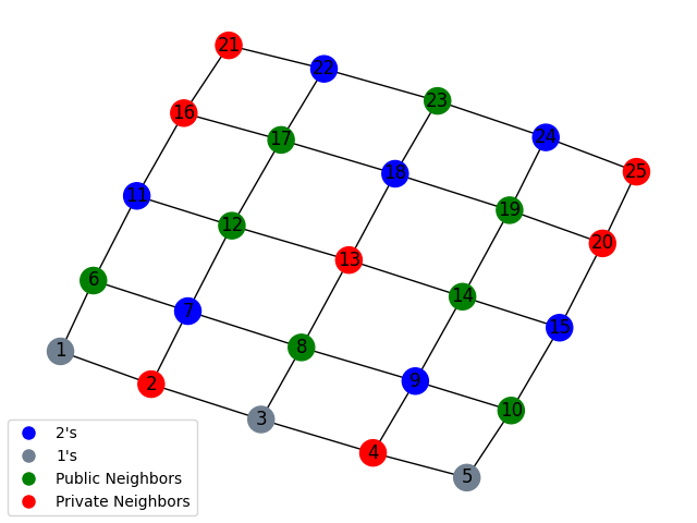
Figure 3.2. Minimum labeling of a $5\times 5$ Grid

Notice the peripheral vertices 1,3, and 5 of Figure 3.2 are the only vertices with a label of 1, and as we continue to make the grid larger, we begin to see a pattern emerge until the peripheral vertices are reached. Given this, our intuition would tell us that a graph with no peripheral vertices; i.e an infinite tiling would produce a “nice” labeling.

3.3. Graphs that Tile the Plane

Chavey [3] provides us with a list of different $k$-regular graphs that tile the plane, three of which we will look at here. We continue our discussion on grid graphs and ask the question of what is the $2RD$ dominating density of an infinite grid graph. It is not as apparent as an infinite path, so we began labeling a finite section of the infinite grid in search of a pattern. Figure 3.3 shows an example of beginning such an optimal labeling. Just as above, green zeroes are public neighbors and red zeroes are private neighbors. Notice that this pattern works for the center of the grid but breaks as you hit the peripheral of the grid.

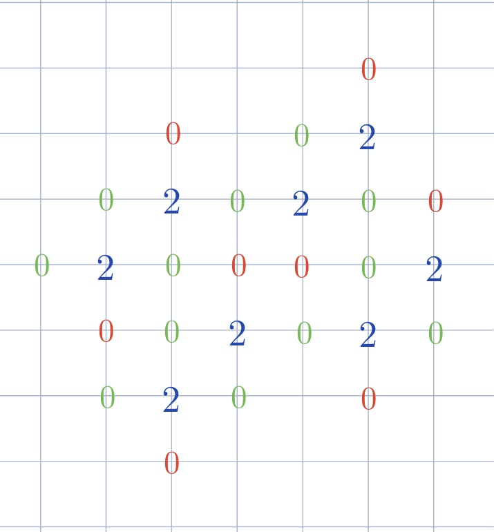
Figure 3.3. Beginning to label an infinite grid graph

Luckily, the bound for dominating density given by Theorem 3.5 provides us with some valuable information and direction. Since the maximum degree of the infinite grid is 4, we conclude $\mathbf{D}(G_{\infty})\geq\frac{4}{7}$. Much like with the $P_{5}$ subgraphs of an infinite path, if we can find a subgraph of the infinite grid which has order 7 and a label sum of 4 which tiles the grid, then we have a minimum labeling.

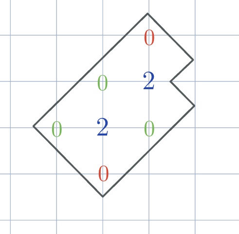
Figure 3.4. Block in infinite grid

Figure 3.4 shows such a subgraph block as described above. In Figure 3.5, we see how this subgraph can tile the infinite grid and produces a valid labeling.

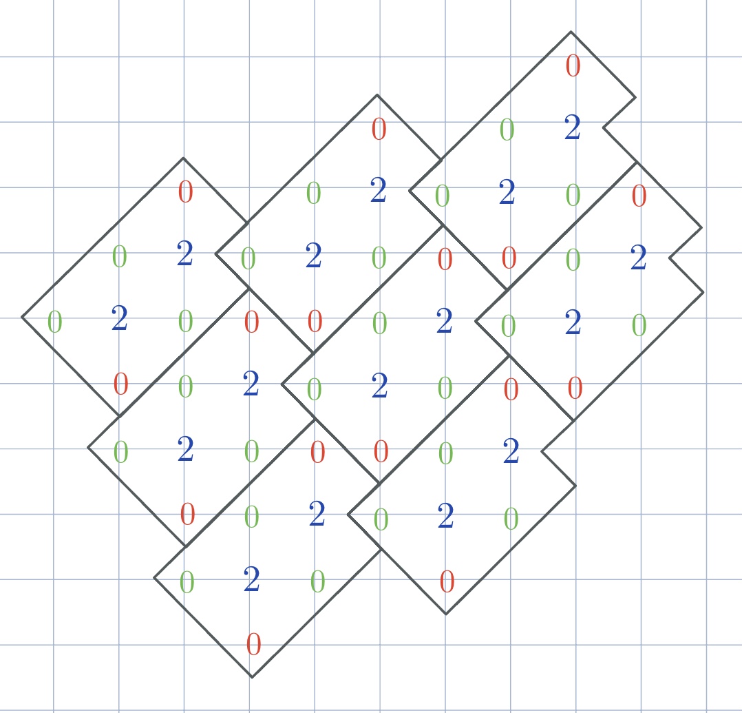
Figure 3.5. Minimum Infinite 4-Regular labeling

We now move to another regular polygon tiling of the plane; a 3-regular hexagonal tiling. Since the labeling pattern is more rigid, we display it in Figure 3.6 and examine two ways to see that the $2RD$ dominating density is indeed the minimum $\frac{2}{3}$.

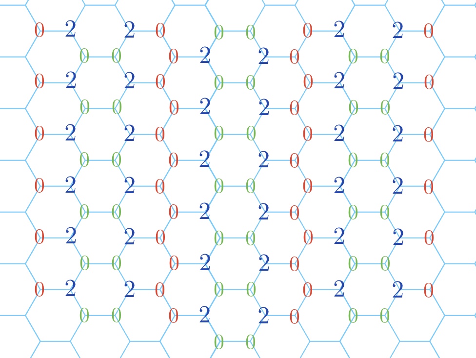
Figure 3.6. Minimum Infinite 3-regular labeling

A quick visual way to verify that the labeling density here is $\frac{2}{3}$ is to consider that every three “columns” there is a pattern of all 0 labels, followed by two columns of alternating 2 and 0 labels. So, if we think of the density of the all 0 label column as 0 and the density of the other two columns as 1, we get a density of $\frac{2}{3}$ every three columns as shown:

$$1\cdot\frac{1}{3}+1\cdot\frac{1}{3}+0\cdot\frac{1}{3}=\frac{2}{3}.$$

Alternatively, we note that the labeling follows a 0-0-0-2-2-0 repeating pattern every row. This can be seen in Figure 3.6 by starting with the left most green 0 label (see Figure 3.7). Thus, a density of $\frac{2}{3}$ (which is the theoretical minimum) is obtained for the entire graph.

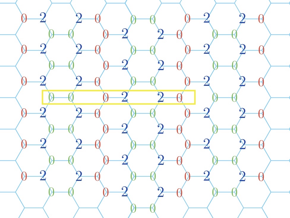
Figure 3.7. Minimum Infinite 3-regular labeling showing repeating pattern with density $\frac{2}{3}$

The third regular polygon tiling of the plane is a 6-regular triangular tiling. A minimum labeling for a 6-regular tiling of the plane os shown in figure 3.8

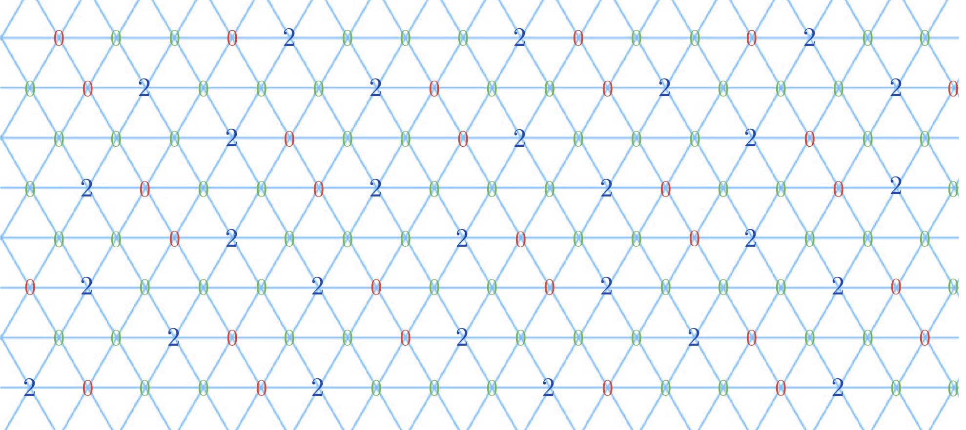
Figure 3.8. Minimum Infinite 6-Regular labeling

We confirm that this labeling pattern realizes the minimum in a similar way to what we did for the 3-regular tiling. Note that the labels that fall along the top left to bottom right diagonals follow a pattern every three “columns.” There is a column of all zeroes followed by a column that has two 0s then a 2 repeating. We also find a horizontal pattern in the labeling of 0-0-0-0-2-0-0-0-2 as seen in Figure 3.9. This pattern repeats to cover the entire plane. So the density will be $\displaystyle\frac{4}{9}$.

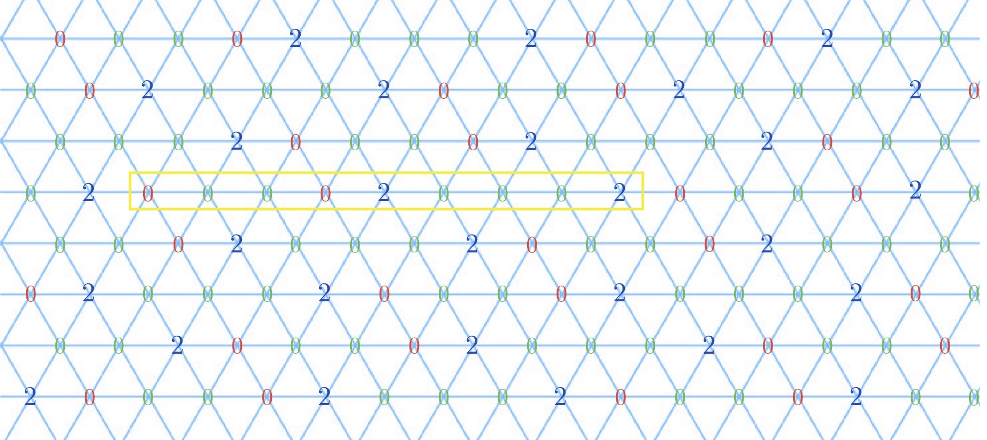
Figure 3.9. Minimum Infinite 6-Regular labeling showing repeating pattern with density $\frac{4}{9}$

Notice that in every infinite graph, we have found a labeling that agrees with the theoretical minimum density for the graph. We have found more complex patterns for labeling other semi-regular tilings of the plane, but these labelings do not reach the theoretical minimum density. We have not been able to prove that their densities simply do not hit the theoretical minimum density, so we cannot show that our labeling is indeed the most optimal. This may be due to the fact that with semi-regular tilings, not all edges incident to a particular vertex are the same. So our choice of labels may vary depending on which edges we use. It may also be that the theoretical minimum is not actually attainable. This would mean that there is “wasted” domination happening on the board. This could be where a vertex does not have an exterior private neighbor.

Chapter 4 Properties, Connections, and Applications

As we continue to explore the various properties and expansions of $2RD$, it is helpful to zoom out and consider how this variation on domination compares with other variations and even with the dominating function itself. In this chapter, we observe such comparisons and in the process uncover more properties. We also consider what real world applications $2RD$ can have, as well as introduce a python program that can assist with such applications. First, we clarify a possible misconception about the nature of minimum-weight labels.

4.1. Exterior Private Neighbors and Minimum Weight Labelings

We have discussed throughout that we typically strive to label a graph such that vertices with label 2 have exterior private neighbors, as it extends the reach that dominating vertices have on the graph. However, this is not always achievable with certain graphs; for example, the graphs in Figure 2.1 and Figure 2.2 both have minimum weight $2RD$ labelings with no $epn$’s. So, we cannot argue that a minimum weight labeling implies 2’s have $epn$’s. But one may want to argue that the converse is true: If every vertex in some $f$ on $G$ with label 2 has an $epn$, then $f$ is a minimum weight labeling. However, we can see that this is not the case in the following example.

Figure 4.1. A labeling on $G$ where every $v\in V_{2}$ has an $epn$

In the graph in Figure 4.1, all three vertices with label 2 have an exterior private neighbor (highlighted in red). However, this labeling is not minimum.

Figure 4.2. A minimum labeling of the graph in Figure 4.1 where no $v\in V_{2}$ has an $epn$

Note the labeling of the graph in Figure 4.2 has a smaller weight than the labeling of the same graph in Figure 4.1 but has no vertices in $V_{2}$ with exterior private neighbors. So, our brief analysis tells us that although exterior private neighbors can be helpful, and in cases result in a minimum labeling, there is no relationship between maximizing the number of 2’s which have $epn$’s and minimizing the weight of the $2RD$ function on a graph.

4.2. Connections To Other Results

Aside from introducing and defining the dominating and Roman Domination functions, we have not returned to these functions in the larger scope of comparing them to our $2RD$ function. We use this section to draw such comparisons.

4.2.1. Maximum Degree Bound

It can be shown simply that given a finite graph $G$ with order $n$, then $\gamma(G)\geq\frac{n}{\Delta(G)+1}$. This is a rather simple concept to understand because every vertex that is in the dominating set is adjacent to at most $\Delta(G)$ vertices, which means that a vertex can dominate at most $\Delta(G)+1$ vertices, which includes itself. Therefore, the minimum number of vertices we need in a dominating set is the order of the graph divided by $\Delta(G)+1$.

While Xu in [6] eventually proves an even better lower bound for Roman Domination, she also proves that $\gamma_{R}(G)\geq\frac{2n}{\Delta(G)+1}$. Now, if we re-write the lower bound for density as shown in Theorem 3.1, we get that $\gamma_{2R}(G)\geq\frac{4n}{\Delta(G)+3}$. Observing these three lower bounds in sequence makes the progression clear, and said progression makes intuitive sense when we unpack how each dominating variant behaves differently than the last. Under Roman Domination, a vertex with label 2 can fully dominate as many vertices as are adjacent to it. Whereas in $2RD$, a vertex with label 2 can only partially dominate as many vertices are adjacent to it, but it needs the help of another vertex of label 2 to make the labeling valid. So, we see how, much like the jump from domination to Roman Domination, we need almost double the amount of dominating vertices to fully $2R$ Dominate our graph. Alas, the extra two vertices in the denominator, as seen more clearly by rewriting the bound for $\gamma_{2R}(G)$ as $\gamma_{2R}(G)\geq\frac{4n}{\Delta(G)+1+2}$ come from the fact that each 2 can fully dominate at most one vertex (their $epn$).

4.2.2. Menger’s Theorem Connection

Throughout our analysis, we introduced two main ways to quantify how the $2RD$ function behaves on a graph. Theorem 2.6 showed that the optimality of a graph was dependent on the maximum number of $eccd$’s that existed in the graph. This idea of counting how many times something happens in a graph to define a global graph property is very important. A similar result is related to counting disjoint paths and the connectivity of a graph; Menger’s Theorem.

Theorem 4.1.

Menger’s Theorem [7]: If $a$ and $b$ are disjoint non-adjacent vertices in a connected graph $G$, then the maximum number of internally disjoint paths connecting $a$ and $b$ is the minimum number of vertices in a set that, when removed from $G$, disconnects $a$ and $b$.

Menger’s Theorem has several important consequences related to the connectivity of a graph. For example, if we let $g(a,b)$ denote the maximum number of internally disjoint paths connecting $a$ and $b$, then the connectivity of $G$ is equal to the maximum $k$ such that $g(x,y)\geq k$ for all $x,y\in V(G)$. So finding a global parameter, connectivity of $G$, comes down to finding the maximum number of disjoint paths between vertices.

Thus Menger’s Theorem shows that connectivity is related to the maximum number of disjoint paths in a graph. Notice that this is almost parallel to the process of finding a minimum $2RD$ labeling by finding the maximum number of $eccd$’s through a graph.

4.3. Applications

Roman Domination was created as a graph theory explanation for why the Roman Empire fell, and a way to quantify how dominating a vertex in the dominating set can be. While Roman Domination assumed there was only one attacker, we created $n$-attack Roman Domination to ask how this graph structure might change if there are $n$ attackers. While army semantics are certainly a real world application, there are other more practical applications that can be extrapolated. One such application is using $2RD$ to help model how and where to place factories, warehouses, and headquarters in a new country. For example purposes, imagine a new company wants to be able to ship all around the country. The headquarters, with more product and staff on hand can ship locally and have a reach to other cities or states nearby. These may represent the 2’s in our $2RD$ graph. The company may also have smaller factories with warehouses that can only ship locally. They do not have the reach of the headquarters, but they can be self-sufficient. These may be represented by 1’s in our graph.

We have constructed a Python program, as seen in Appendix II, which can provide the optimal $2RD$ labeling of a given graph. To further extend our analogy, assume that building headquarters is much more expensive than smaller factories, so the company wants to limit itself to three headquarters. The program also has a feature (we call finite resources) to provide the minimum labeling given an added limitation on the number of 2’s you are allowed to use.

4.3.1. Using The Programs

As mentioned in the section above, it is not always trivial to find the minimum weight labeling for certain graphs, especially when order gets large. In fact, given a labeling, it is not always easy to decide whether the said labeling is valid or not. When we began our research we found many programs exist to tell you whether a graph’s labeling is a valid dominating labeling. However, no such program exists to decide whether a labeling is a valid Roman Domination labeling. Appendix I does just that. The code in Appendix II can be modified to do this, but it is actually a much more robust program. Using the method outlined in Corollary 2.8, the program in Appendix II outputs and displays the minimum $2RD$ labeling of a graph.

Provide the program in Appendix I with a txt file like the example graph in Appendix IIIa, where the categories separated by semicolons are as follows “vertex number: label: adjacencies”. The program then outputs whether the current labeling is valid or not. For the $2RD$ labeling program in Appendix II, provide it with a txt file like the example graph in Appendix IIIb, where the categories separated by semicolons are vertex number: label (we are giving the program an unlabeled graph so make this an arbitrary -1): adjacencies. When the program is running, a terminal similar to the one displayed in Appendix IIIc will allow the user to customize the type of analysis they wish to run on the given graph (see Section 5.1 for more). Note that much refactoring has been done to increase the maximum order graph that the program can handle (which is about 30-40 depending on the size of the graph). The program can be modified to give bounds for very large order graphs.

Chapter 5 Conclusion

In our analysis, we expanded upon a well-studied variation of the dominating function, Roman Domination. While our analysis mainly dove into $2$-attack Roman Domination, we have defined it for a general $n$ case. In Chapter 2, we discussed the classification we call optimality to measure how “good” we can label a graph. In Chapter 3, we note that said optimality is helpful for finite graphs, but we need a different type of classification for infinite graphs. We used $2RD$ density and the proven lower bound to decide whether the infinite labelings we found for such graphs were minimum. In Chapter 4, we related our findings back to Roman Domination, and domination itself, as well as other graph theory properties that use similar techniques. We also introduced a program which provides different minimum labelings of a given graph.

5.1. Future Work

As mentioned above, we defined a general $n$-attack Roman Domination variation. As we only explored the 2-attack case, a natural continuation of the problem would be to analyze whether the properties and methods we discussed can be augmented to fit higher attack cases. Furthermore, the algorithmic way to find a minimum labeling described in Corollary 2.8 does so in a very particular way. The algorithm will always output the minimum labeling with the fewest number of 2’s used. For example, observe $P_{4}$ below with two minimum labelings.

Figure 5.1. Two minimum labelings

The algorithm will always output the left labeling. If we call this type of labeling optimal 2-minimized, we naturally ask if there is a similar formula that obtains the optimal 2-maximized labeling. Our program, shown in Appendix II, which uses aspects of the algorithm can find both the $2RD$ 2-minimized and 2-maximized minimum labelings of a graph through brute force. Applicationally speaking, if limiting the number of 2’s is the goal, the optimal 2-minimized labeling is preferred. But fewer 2’s means more overall dominating vertices, so if you want the dominating set to be as small as possible, an optimal 2-maximized labeling is preferred. Note that a $P_{4}$ can also be labeled $0-2-1-1$, which is yet another minimum weight labeling. So, a $P_{4}$ can be minimally labeled using zero, one, or two 2’s. However, if we consider a $K_{6,6}$, as shown in Figure 2.2, minimum weight labelings exist using two or four 2’s; however, there is no minimum weight labeling we can create that uses three 2’s. Using the two customization options in the $2RD$ program, we can find all possible minimum weight labelings. Other continuations of our problem could include deducing which graphs, or which graph properties, lead to certain minimum weight labelings existing.

As explained in Section 3.3, there are certain semi-regular tilings of the plane for which we have not been able to find a minimum labeling for, as their density does not hit the theoretical lower bound. However, we have not been able to argue if and why certain semi-regular tilings simply cannot hit this bound. This is another possible continuation of the problem. Similar to infinite tilings, we could also explore fractal graphs such as the Sierpinski Triangle. Figure 5.2 depicts the minimum weight $2RD$ labeling for the $3\textsuperscript{rd}$ iteration of the Triangle.

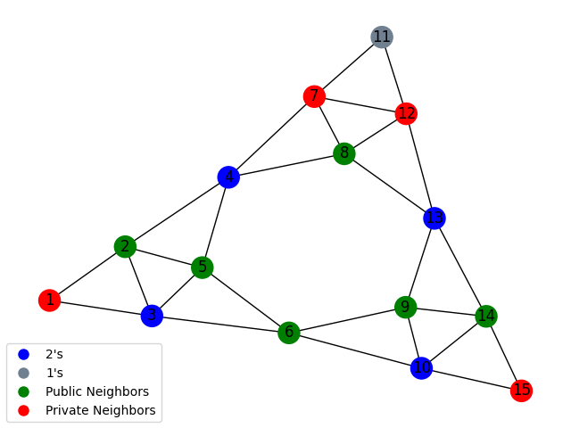
Figure 5.2. Minimum labeling of $3\textsuperscript{rd}$ iteration of the Sierpinski Triangle

The program tells us that the 2-minimized and 2-maximized $2RD$ labelings are the same, which indicates that the labeling in Figure 5.2 is unique. Further research could continue examining the later iterations of the Triangle to find a labeling pattern, or even to find if later iterations also have unique labelings.

There are many possible continuations to our problem, either through exploring new graph classes, different infinite tilings, or even examining higher attack cases. Many applications exist for these extensions, which make them practical problems to study.

Appendix

Appendix I
$RD$ Validation

⬇

1"""

2This program takes a LABELED graph and determines whether it follows the rules for Roman Domination. It also

3returns a graphical representation color-coded by vertex labelling.

4

5Code by Garrison Koch

6"""

7import matplotlib.pyplot as plt

8import networkx as nx

9

10

11def read_graph(filename):

12 """

13 This is the function that reads the .txt file and converts it into two comprehensive dictionaries that store the information

14 needed for the rest of the program to interpret and

15 :param filename: .txt graph

16 :return: two dictionaries: one of the vertices with their labels (this will currently be -1 for every vertex but will get updated

17 the other dict has the graphs vertices as the keys and the vertices that key is adjacent to are the values

18 """

19 file = open(filename)

20 labels = {}

21 graph_adjacencies = {}

22 for line in file:

23 line = line.strip()

24 vertex, label, adjacencies = line.split(’:’)

25 vertex = int(vertex)

26 label = int(label)

27 if len(adjacencies) > 0:

28 adjacencies = adjacencies.split(’,’)

29 for i in range(len(adjacencies)):

30 adjacencies[i] = int(adjacencies[i])

31 labels[vertex] = label

32 graph_adjacencies[vertex] = adjacencies

33 return labels, graph_adjacencies

34

35

36def is_RD(labels, graph_adjacencies):

37 """

38 This function takes the labels and adjacencies of the graph and determines whether it follows the Roman Dominating

39 rules.

40 It returns true if the graph is properly Roman Dominated and False if it is not.

41 """

42 for item in labels:

43 dominated = 1

44 if labels[item] == 0:

45 dominated = 0

46 for adjacency in graph_adjacencies[item]:

47 if labels[adjacency] == 2:

48 dominated += 1

49 if dominated == 0:

50 return False

51 return True

52

53

54def graph_in_nx(graph_labels, graph_adjacencies):

55 """

56 This function graphs the given graph with the updated labels. It color codes the vertices for ease of viewing.

57 """

58 edge_list = []

59 for item in graph_adjacencies:

60 for i in range(len(graph_adjacencies[item])):

61 edge_list.append((item, graph_adjacencies[item][i]))

62 G = nx.Graph()

63 for i in range(1, len(graph_adjacencies)):

64 G.add_node(i)

65 for edge in edge_list:

66 G.add_edge(*edge)

67 color_key = []

68 for node in G:

69 if graph_labels[node] == 0:

70 color_key.append(’red’)

71 elif graph_labels[node] == 2:

72 color_key.append(’green’)

73 else:

74 color_key.append(’blue’)

75 plt.figure()

76 nx.draw(G, labels=graph_labels, node_color=color_key, with_labels=True)

77 plt.show()

78

79

80def main():

81 graph_selection = input(’Enter your graph name (with .txt at end): ’)

82 labels, adjacencies = read_graph(graph_selection)

83 print(f’Under the labelling {labels}’)

84 x = is_RD(labels, adjacencies)

85 if x:

86 print(’This is a valid Roman Domination labelling’)

87 else:

88 print(’This is not a valid Roman Domination labelling’)

89 graph_in_nx(labels, adjacencies)

90

91

92if __name__ == "__main__":

93 main()

Appendix II
$2RD$ Minimum labeling

⬇

1"""

2This program takes an unlabelled graph and returns 2-attack roman dominating number and the most optimal labeling

3that realises this dominating number. You can also do the "limited resource" mode which emulates only wanting to

4place n number of headquarters. It also renders the graph with color coded vertices and labels.

5

6Code by Garrison Koch

7"""

8

9import matplotlib.pyplot as plt

10from matplotlib.lines import Line2D

11import networkx as nx

12import time

13import itertools

14

15

16def read_graph(filename):

17 """

18 This is the function that reads the .txt file and converts it into two comprehensive dictionaries that store the information

19 needed for the rest of the program to interpret and

20 :param filename: .txt graph

21 :return: two dictionaries: one of the vertices with their labels (this will currently be -1 for every vertex but will get updated

22 the other dict has the graphs vertices as the keys and the vertices that key is adjacent to are the values

23 """

24 file = open(filename)

25 labels = {}

26 graph_adjacencies = {}

27 for line in file:

28 line = line.strip()

29 vertex, label, adjacencies = line.split(’:’)

30 vertex = int(vertex)

31 label = int(label)

32 if len(adjacencies) > 0:

33 adjacencies = adjacencies.split(’,’)

34 for i in range(len(adjacencies)):

35 adjacencies[i] = int(adjacencies[i])

36 labels[vertex] = label

37 graph_adjacencies[vertex] = adjacencies

38 file.close()

39 return labels, graph_adjacencies

40

41

42def all_supply_sets_minimized(labels, supplies):

43 """

44 This function finds all sets of the vertices with supply_size supply down to 0. It returns a list of lists of all

45 possible dominating sets with size supply_size down to 0.

46 """

47 supply_sets = []

48 supply_size = min(len(labels) // 2 + 1, supplies) # The largest supply size will ever need to be

49 for i in range(0, supply_size + 1):

50 supply_sets_of_size_i = list(

51 itertools.combinations(labels.keys(), supply_size - i)) # goes from largest to smallest "two sets"

52 for item in supply_sets_of_size_i:

53 supply_sets.append(item)

54 return supply_sets

55

56

57def all_supply_sets_maximized(labels, supplies):

58 """

59 This function finds all sets of the vertices with supply_size supply down to 0. It returns a list of lists of all

60 possible dominating sets with size 0 up to supply_size.

61 """

62 supply_sets = []

63 supply_size = min(len(labels) // 2 + 1, supplies) # The largest supply size will ever need to be

64 for i in range(0, supply_size + 1):

65 supply_sets_of_size_i = list(

66 itertools.combinations(labels.keys(), i)) # goes from smallest to largest "two sets"

67 for item in supply_sets_of_size_i:

68 supply_sets.append(item)

69 return supply_sets

70

71

72def list_intersection(list1, list2):

73 """

74 This function returns the intersection of two lists

75 """

76 intersection = []

77 for item in list1:

78 if item in list2:

79 intersection.append(item)

80 return intersection

81

82

83def find_neighborhoods(adjacencies, supply_set):

84 """

85 This function takes a set of vertices and finds their public neighborhood (vertices adjacent to at least 2

86 vertices in the set) and their private neighborhood (only one per vertex in set). It returns the public neighborhood

87 as a list, and the private neighbors as a dictionary where the keys are vertices in the set and the values are their

88 unique private neighbor if they have one.

89 """

90 public_neighborhood = []

91 private_neighbors = {}

92

93 if len(supply_set) == 0:

94 return public_neighborhood, private_neighbors

95 for vertex in adjacencies:

96 if vertex not in supply_set and len(list_intersection(adjacencies[vertex], supply_set)) >= 2:

97 public_neighborhood.append(vertex)

98 for vertex in adjacencies:

99 if vertex not in supply_set and len(list_intersection(adjacencies[vertex], supply_set)) == 1:

100 for item in adjacencies[vertex]:

101 if item in supply_set:

102 private_neighbors[item] = vertex

103

104 return public_neighborhood, private_neighbors

105

106

107def number_saved(public, private, current_set):

108 """

109 This function computes the difference in the sum of the labels and the number of vertices in the graph. We want this

110 number to be as large as possible

111 """

112 saved = len(public) + len(private) - len(current_set)

113 return saved

114

115

116def find_optimal_set(labels, adjacencies, supply_count, supply_style):

117 """

118 This is the head function that carries out the finding of the most optimal labeling and returns the "labels"

119 dictionary with the updated labels.

120 """

121 if supply_style == 2:

122 supply_sets = all_supply_sets_maximized(labels, supply_count) ## CHANGE FOR MAXIMIZED

123 else:

124 supply_sets = all_supply_sets_minimized(labels, supply_count)

125 two_set = []

126 two_set_public, two_set_private = find_neighborhoods(adjacencies, two_set)

127 for supply_set in supply_sets:

128 public, private = find_neighborhoods(adjacencies, supply_set)

129 if number_saved(public, private, supply_set) >= number_saved(two_set_public, two_set_private, two_set):

130 two_set = supply_set

131 two_set_public, two_set_private = find_neighborhoods(adjacencies, two_set)

132 if len(two_set) > 0:

133 print(f’The most optimal set of vertices with label 2 will be: {list(two_set)}’)

134

135 ## Making Labels ##

136

137 zero_set = []

138 for item in two_set_public:

139 zero_set.append(item)

140 for item in two_set_private.values():

141 zero_set.append(item)

142 for vertex in labels:

143 if vertex in two_set:

144 labels[vertex] = 2

145 elif vertex in zero_set:

146 labels[vertex] = 0

147 else:

148 labels[vertex] = 1

149 return labels, two_set_public, two_set_private

150

151

152def find_TwoRD_number(new_labels):

153 twoRD_number = 0

154 for label in new_labels.values():

155 twoRD_number += label

156 return twoRD_number

157

158

159def graph_in_nx(graph_labels, public, private, graph_adjacencies):

160 """

161 This function graphs the given graph with the updated labels. It color codes the vertices for ease of viewing.

162 """

163 edge_list = []

164 for item in graph_adjacencies:

165 for i in range(len(graph_adjacencies[item])):

166 edge_list.append((item, graph_adjacencies[item][i]))

167 G = nx.Graph()

168 for i in range(1, len(graph_adjacencies)):

169 G.add_node(i)

170 for edge in edge_list:

171 G.add_edge(*edge)

172 color_key = []

173 for node in G:

174 if graph_labels[node] == 0 and node in public:

175 color_key.append(’green’)

176 elif graph_labels[node] == 0 and node in private.values():

177 color_key.append(’red’)

178 elif graph_labels[node] == 2:

179 color_key.append(’blue’)

180 else:

181 color_key.append(’slategray’)

182 plt.figure()

183 nx.draw(G, node_color=color_key, with_labels=True)

184 # To make legend #

185 legend_elements = [Line2D([0], [0], marker=’o’, color=’w’, label=’2\’s’,

186 markerfacecolor=’blue’, markersize=10),

187 Line2D([0], [0], marker=’o’, color=’w’, label=’1\’s’,

188 markerfacecolor=’slategray’, markersize=10),

189 Line2D([0], [0], marker=’o’, color=’w’, label=’Public Neighbors’,

190 markerfacecolor=’green’, markersize=10),

191 Line2D([0], [0], marker=’o’, color=’w’, label=’Private Neighbors’,

192 markerfacecolor=’red’, markersize=10)]

193 plt.legend(handles=legend_elements, loc=’lower left’)

194 plt.show()

195

196

197## Below here is for user interaction, to decide what they want to do and pick which graph they would like to look at ##

198def ask_multiple_choice_question(question, options):

199 """

200 This is the input validation for multiple choice questions. It will only accept answer choices that are choices

201 for the question.

202 """

203 print(question)

204 answers = [’1’, ’2’]

205 available_answers = answers[0:len(options)]

206 for i in range(len(options)):

207 print(f’{answers[i]}. {options[i]}’)

208 answer = input("Enter your choice: ").lower()

209 while answer not in available_answers:

210 answer = input(’That\’s not an option. Try again: ’).lower()

211 return answer

212

213

214def limited_resources(labels):

215 """

216 This function asks the user whether they would like to find the 2-attack RD number or observe the 2RD labelling

217 and number if you are only allowed to place a limited number of 2’s (headquaters) i.e., how many supplies you

218 would like to allow.

219 Note that you will never allow more supplies than you have vertices.

220 """

221 response = ask_multiple_choice_question(’Which type of analysis would you like to conduct on this graph?’,

222 [’Unlimited Resources (Just find 2-attack RD number)’, ’Limited Resources’])

223 if response == ’1’:

224 return len(labels)

225 else:

226 supplies = input(’How many resources (supplies) would you like to allow? ’)

227 while not supplies.isdigit() or int(supplies) < 1 or int(supplies) > len(labels):

228 supplies = input(’Invalid. How many resources (supplies) would you like to allow? ’)

229 return int(supplies)

230

231

232def dominating_style(labels):

233 """

234 This function asks the user whether they would like to find the minimum labeling using 2RD 2-minimized or 2RD

235 2 - maximized

236 """

237 response = ask_multiple_choice_question(’Which dominating style would you like to use?’,

238 [’2RD 2-minimized’, ’2RD 2-maximized’])

239 if response == ’1’:

240 return 1

241 else:

242 return 2

243

244

245def main():

246 graph_selection = input(’Enter your graph name (with .txt at end): ’)

247 labels, adjacencies = read_graph(graph_selection)

248 supply_selection = limited_resources(labels)

249 supply_style = dominating_style(labels)

250 new_labels1, public1, private1 = find_optimal_set(labels, adjacencies,

251 supply_selection,

252 supply_style)

253 print(’The optimal vertex labels: ’, new_labels1)

254 print(’The 2-attack Roman Dominating number is:’, find_TwoRD_number(new_labels1))

255 time.sleep(1)

256 graph_in_nx(new_labels1, public1, private1, adjacencies)

257

258

259if __name__ == "__main__":

260 main()

Appendix IIIa
$RD$ Graph

⬇

11:2:2,3,4,5

22:0:1

33:0:1

44:0:1

55:0:1

66:0:7

77:1:6

Appendix IIIb
$2RD$ Graph

⬇

11:-1:2,3

22:-1:1,3,4

33:-1:1,2,5

44:-1:2,5,7,8

55:-1:2,3,4,6

66:-1:3,5,9,10

77:-1:4,8,11,12

88:-1:4,7,12,13

99:-1:6,10,13,14

1010:-1:6,9,14,15

1111:-1:7,12

1212:-1:7,8,11,13

1313:-1:8,9,12,14

1414:-1:9,10,13,15

1515:-1:10,14

Appendix IIIc
Example terminal and output for $2RD$ program

Bibliography

- [1] R. A. Beeler, T. W. Haynes, and S. T. Hedetniemi. Double Roman domination. Discrete Appl. Math., 211:23–29, 2016.
- [2] F. Buckley and M. Lewinter. Introductory Graph Theory with Applications. Waveland Press, Long Grove, IL, 2013.
- [3] D. Chavey. Tilings by regular polygons—ii: A catalog of tilings. Computers and Mathematics with Applications, 17(1):147–165, 1989.
- [4] E. J. Cockayne, O. Favaron, and C. M. Mynhardt. Secure domination, weak Roman domination and forbidden subgraphs. Bull. Inst. Combin. Appl., 39:87–100, 2003.
- [5] T. W. Haynes and M. A. Henning. Total domination good vertices in graphs. Australas. J Comb., 26:305–, 2002.
- [6] X. Linfeng. Roman domination. http://math.uchicago.edu/~may/REU2015/REUPapers/Xu,Linfeng.pdf, 2015. [Online; accessed 10-January-2023].
- [7] K. Menger. Zur allgemeinen kurventheorie. Fundamenta Mathematicae, 10(1):96–115, 1927.
- [8] Z. Shao, S. Klavžar, Z. Li, P. Wu, and J. Xu. On the signed Roman -domination: complexity and thin torus graphs. Discrete Appl. Math., 233:175–186, 2017.