Hadronic Structure, Conformal Maps, and Analytic Continuation

Abstract

We present a method for analytic continuation of retarded Green functions, including Euclidean Green functions computed using lattice QCD. The method is based on conformal maps and construction of an interpolation function which is analytic in the upper half plane. A novel aspect of our treatment is rigorous bounding of systematic uncertainties, which are handled by constructing the full space of interpolating functions (at each point in the upper half-plane) consistent with the given Euclidean data and the constraints of analyticity. The resulting Green function in the upper half-plane has an appealing interpretation as a smeared spectral function.

I Introduction

Current-current correlation functions in quantum chromodynamics (QCD) encode fundamental features of hadronic structure. For example, the hadronic vacuum polarization tensor is defined as the vacuum expectation value of the commutator of the electromagnetic currents [1, 2]:

$$\rho_{\mu\nu}(q) =\frac{1}{2\pi}\int d^{4}x\,e^{iq\cdot x}\langle\emptyset|[j_{\mu}^{\rm EM}(x),j_{\nu}^{\rm EM}(0)]|\emptyset\rangle,$$ (1)

with $\rho_{\mu\nu}(q)=(q_{\mu}q_{\nu}-q^{2}g_{\mu\nu})\rho(q^{2})$, where $\rho(q^{2})$ is the spectral density. The spectral density is related to the experimentally measured $R$-ratio,

$$\rho(s)=\frac{R(s)}{12\pi^{2}} R(s)=\frac{\sigma(e^{+}e^{-}\to{\rm hadrons})}{4\pi\alpha^{2}/3s},$$ (2)

where the denominator is the tree-level QED cross section for $e^{+}e^{-}\to\mu^{+}\mu^{-}$ in the massless limit ($m_{\mu}^{2}\ll s$). The experimental data for $R(s)$, reproduced in Fig. 1 from the compilation of Ref. [3], show a rich resonance structure, with prominent peaks near the masses of vector resonances. These resonant peaks are the hadronic structure of the vacuum polarization.

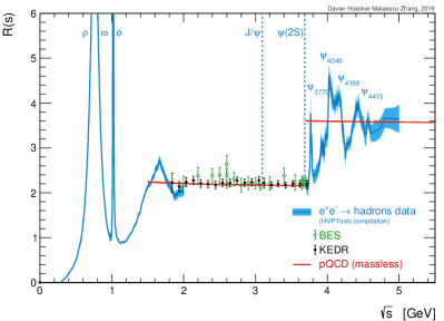
Figure 1: Compilation of experimental data for $R(s)$, reproduced with permission from Ref. [3].

The hadronic tensor of unpolarized inclusive electron-proton scattering has a similar form [4],

$$W_{\mu\nu}(p,q)=\int\frac{d^{4}x}{4\pi}e^{iq\cdot x}\langle p|[j_{\mu}^{\rm EM}(x),j_{\nu}^{\rm EM}(0)]|p\rangle,$$ (3)

where the external states correspond to a proton with four-momentum $p$ and $q=k-k^{\prime}$ is the momentum transfer between the initial and final electrons with momenta $k$ and $k^{\prime}$, respectively. The Lorentz covariant decomposition of the hadronic tensor is given by

$$\begin{split}W_{\mu\nu}&=F_{1}\left(-g_{\mu\nu}+\frac{q_{\mu}q_{\nu}}{q^{2}}\right)\\ &+\frac{F_{2}}{p\cdot q}\left(p_{\mu}-\frac{p\cdot qq_{\mu}}{q^{2}}\right)\left(p_{\nu}-\frac{p\cdot qq_{\nu}}{q^{2}}\right),\end{split}$$ (4)

where $F_{1}$ and $F_{2}$ are so-called structure functions. Similar to the case of the hadronic vacuum polarization above, $F_{1}$ and $F_{2}$ can also be interpreted as spectral densities. Moreover, as shown in Fig. 2 for $F_{2}$, the experimentally measured structure functions exhibit conspicuous resonant peaks. These structures encode the non-perturbative response of the proton to electromagnetic probes. To date, essentially no first-principles understanding (e.g., from lattice QCD) of the structure functions exists in the resonance region. For neutrino-nucleon scattering at similar energies, the analogue of Eq. 3 arises with flavor-changing vector and axial currents. Compared to the electromagnetic case, the axial structure functions are especially poorly known. Improved understanding of the axial structure functions would have important consequences for upcoming neutrino experiments like DUNE.

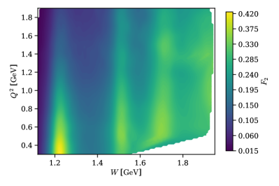
Figure 2: Interpolation of experimental data, taken from the CLAS Physics Database [5], for the structure function $F_{2}$ in the resonance region as a function of the momentum transfer $Q^{2}$ and the invariant mass $W$ of the hadronic system. Large resonant contributions are clearly visible states including $\Delta(1232)$ $N(1520)$, $N(1535)$, and $N(1720)$. In Ref. [6], at least a dozen open channels were used to model the experimental data.

Euclidean-time analogues of Eqs. 2 and 3 are calculable using lattice QCD. Extracting a spectral density from a zero-temperature Euclidean correlation function $\mathscr{G}_{E}(\tau)$ requires inverting a Laplace transform,

$$\mathscr{G}_{E}(\tau)=\int_{0}^{\infty}d\omega\,e^{-\omega\tau}\rho(\omega).$$ (5)

Lattice QCD calculations provide $\mathscr{G}_{E}(\tau)$ at a discrete set of Euclidean times. Without further assumptions, this problem is famously ill posed. Efforts to solve Eq. 5 have typically focused on the Laplace transform’s structure as a linear integral equation, approximated by the discretized linear system $\mathscr{G}_{E}(\tau_{i})=K_{ij}\rho(\omega_{j})$ where $K_{ij}=\int d\omega\,e^{-\tau_{i}\omega_{j}}$ and summation is implied. Suitably regularized linear methods are then employed to extract the spectral density. Much recent interest in the lattice community has been generated by the inversion algorithm of Ref. [7], independently rediscovered and applied to lattice gauge theory for the first time in Ref. [8]. The general inverse problem has seen many approaches a broad literature spanning many fields [9, 10, 11, 12, 13, 14, 15, 16, 17, 18, 19, 20, 21, 22, 23, 24, 25, 26]; existing approaches used in the lattice community have recently been reviewed in Refs.  [27, 28, 29].

Equation 5 amounts to analytic continuation, a connection which is particularly clear in frequency space (see Section III below),

$$G(i\omega_{\ell})=\int_{0}^{\beta}d\tau e^{i\omega_{\ell}\tau}\mathscr{G}_{E}(\tau),$$ (6)

where the retarded Green function on the left-hand side is evaluated on the positive imaginary axis. Meanwhile, the spectral density is related to its imaginary part evaluated on the positive real axis: $\rho(\omega)=\frac{1}{\pi}\operatorname{Im}G(\omega)$. Therefore, the task of analytic continuation is to compute the behavior of $G(z)$ on the real line given finite data on the positive imaginary axis.

In the present work, we propose a method for solving this problem which differs from familiar approaches in three important regards. First, the method is inherently nonlinear, based on special properties of certain conformal maps. Second, the method works by constraining the behavior of $G(\omega+i\epsilon)$ directly in the upper half-plane, with the spectral density arising in the limit $\epsilon\to 0^{+}$. Third, the method explicitly constructs, at each point in the upper half-plane, the full space of analytic functions consistent with the given Euclidean data. Intuitively, one anticipates that this space ought to be small for points near the Euclidean data on the positive imaginary axis and large for points on the real line, where the problem becomes ill posed. At each point $z\in\mathbb{C}^{+}$, this bounding space gives a rigorous bound on the systematic uncertainty associated with the analytic continuation.

The fact that lattice QCD calculations occur in a finite spatial volume raises important conceptual questions. Ref. [30] has convincingly argued that infinite-volume spectral densities may, as a matter of principle, be recovered from finite-volume calculations via the ordered limiting procedure

$$\rho(\omega) =\lim_{\epsilon\to 0}\lim_{L\to\infty}\int d\omega^{\prime}\,\delta_{\epsilon}(\omega,\omega^{\prime})\rho_{L}(\omega^{\prime})$$ (7)

$$\equiv\lim_{\epsilon\to 0}\lim_{L\to\infty}\rho^{\epsilon}_{L}(\omega),$$ (8)

where $\rho_{L}(\omega)$ is a finite-volume spectral density, $\rho^{\epsilon}_{L}(\omega)$ is a smeared spectral density, and $\delta_{\epsilon}(\omega,\omega^{\prime})$ is a smearing kernel. An important practical upshot is that computing smeared spectral densities is typically a well-posed, albeit numerically delicate, problem. Below we show that analytic continuation at a finite distance $\epsilon$ above the real line has a natural interpretation in terms of a smeared spectral density. Essentially the same point seems to have been observed in Ref. [31], where the usual $i\epsilon$ prescription for computing scattering amplitudes was replaced by a suitable smearing in a proposal to compute scattering amplitudes using lattice gauge theory.

Recently a similar set of ideas to the method we propose was applied to fermionic thermal Green functions in the context of condensed matter problems [32, 33]. Bosonic Green functions are of particular interest in lattice gauge theory. One approach to bosonic Green functions has been given in Ref. [34]. The present work gives an alternative treatment of bosonic Green functions. Our rigorous treatment of the uncertainty in the analytic continuation is another novel feature of the present work.

The rest of this article is organized as follows. Section II reviews some well-known analytic properties of thermal Green functions in the upper half-plane. Section III specializes the results of Section II to the case of a finite spatial volume, where the spectrum is discrete. Section IV transforms, by suitable conformal maps, the problem of analytic continuation from the upper half-plane to the open unit disk. Section V constructs a rational-function approximation for $G(z)$ using the theory of Nevanlinna–Pick interpolation; Section V.4 collects the technical pieces and summarizes the complete algorithm for the method. Section VI provides a recipe for computing $G(i\omega_{\ell})$ given values for $\mathscr{G}_{E}(\tau)$, e.g., from a lattice QCD calculation. Section VII provides a series of numerical examples illustrating how the new method works in practice. Section VIII provides some discussion of the results and presents our conclusions.

II Thermal Green functions in the complex plane

Consider a finite-temperature quantum field theory defined by an equilibrium density matrix

$$\hat{\rho}=\frac{1}{\mathcal{Z}}e^{-\beta H},$$ (9)

with partition function $\mathcal{Z}$, Hamiltonian $H$, and inverse temperature $\beta$. Expectation values are defined with respect to the density matrix as $\langle\mathcal{O}_{1}\dots\mathcal{O}_{n}\rangle\equiv\operatorname{Tr}\left\{\hat{\rho}\,\mathcal{O}_{1}\dots\mathcal{O}_{n}\right\}$. Although many applications of interest occur at zero temperature, the formalism we present holds for arbitrary temperatures. Moreover, as a matter of principle, lattice QCD calculations employ large but finite $\beta$.

Let $A$ be an operator. We define the following correlation functions

$$\mathscr{G}(t) =\langle A(t)A^{\dagger}(0)\rangle,$$ (10)

$$\mathscr{G}_{\pm}(t) =i\langle\{A(t),A^{\dagger}(0)\}_{\pm}\rangle,$$ (11)

where the commutator $(-)$ arises for bosonic operators, while the anti-commutator $(+)$ is for fermionic operators. The Euclidean Green function is defined via analytic continuation to the lower-half plane as

$$\mathscr{G}_{E}(\tau)\equiv\mathscr{G}(-i\tau),$$ (12)

where $\tau\in\mathbb{R}$ is the Euclidean time. The retarded, or causal, correlator is defined as

$$G_{\pm}(\omega) \equiv\int_{0}^{\infty}dt\,e^{i\omega t}\mathscr{G}_{\pm}(t).$$ (13)

Nominally, $\omega$ is a real number. When $\omega$ is replaced by a complex number, Eq. 13 defines an analytic function $G_{\pm}(z)$ in the upper half plane, $\operatorname{Im}z>0$. The retarded correlator plays a key role in linear response theory [35]; its importance to the current discussion arises from its close connection to the Euclidean correlator. The Fourier coefficients of the Euclidean correlator are defined as

$$G_{E}^{(\ell)}\equiv\int_{0}^{\beta}d\tau\,e^{i\omega_{\ell}\tau}\mathscr{G}_{E}(\tau),$$ (14)

where the $\omega_{\ell}$ are the Matsubara frequencies, $2\ell\pi/\beta$ for bosons and $(2\ell+1)\pi/\beta$ for fermions, with $\ell\in\mathbb{Z}$. In Section III below, we will rederive the familiar result that

$$G_{E}^{(l)}=G_{\pm}(i\omega_{\ell}),\,\ell\neq 0.$$ (15)

In other words, the analytic continuation of the retarded correlator is the frequency-space Euclidean correlator.

Finally, the spectral density is defined as

$$\rho_{\pm}(\omega) =\frac{1}{2\pi i}\int_{-\infty}^{\infty}dt\,e^{i\omega t}\mathscr{G}_{\pm}(t)$$ (16)

$$=\frac{1}{2\pi i}\left(G_{\pm}(\omega)-G_{\pm}(\omega)^{*}\right)$$ (17)

$$=\frac{1}{\pi}\operatorname{Im}G_{\pm}(\omega),\,\omega\in\mathbb{R}.$$ (18)

where the second line follows using time-translation invariance and the reality condition. The final line gives the familiar result: for diagonal correlators, the spectral density is the imaginary part of the retarded Green function.

Symbol	Description	Definition
$\mathscr{G}(t)$	Real-time Green function	Eq. 11
$\mathscr{G}_{E}(\tau)$	Euclidean-time Green function	Eq. 12
$G(\omega)$	Retarded Green function, $\omega\in\mathbb{R}$	Eq. 13
$G(z)$	Retarded Green function, $z\in\mathbb{C}^{+}$	Eq. 13
$\mathcal{G}(z)$	Retarded Green function, $z\in\mathbb{D}$	Eqs. 33 and 35

Table 1: The different Green functions appearing in this work. Bosonic and fermionic Green functions are distinuished by the sign of the commutator or anti-commutator, e.g., $G_{\pm}(z)$.

III Finite-volume Green functions

The definitions of the preceding section were generic, in the sense that they made no particular assumption about the dynamics or spectrum of the theory. We now specialize to the case of a thermal field theory in a finite spatial volume $V=L^{3}$, for which the spectrum is discrete.

Inserting complete sets of states in Eq. 11 gives

$$\mathscr{G}_{\pm}(t) =\frac{i}{\mathcal{Z}}\sum_{n,m}e^{-iE_{nm}t}|A_{mn}|^{2}\left(e^{-\beta E_{m}}\pm e^{-\beta E_{n}}\right),$$ (19)

where $E_{mn}\equiv E_{m}-E_{n}$ and $A_{mn}\equiv\langle m|A|n\rangle$. Similarly, the retarded correlator in the upper half-plane $z\in\mathbb{C}^{+}$ becomes

$$G_{\pm}(z)=\frac{1}{\mathcal{Z}}\sum_{n,m}|A_{mn}|^{2}\left(e^{-\beta E_{m}}\pm e^{-\beta E_{n}}\right)\frac{-1}{z-E_{nm}},$$ (20)

where we have used

$$\int_{0}^{\infty}dt\,e^{izt}e^{-iE_{nm}t}=\frac{i}{z-E_{nm}}$$ (21)

for $E_{mn}\in\mathbb{R}$ and $z\in\mathbb{C}^{+}$. This confirms the statement from above that $G_{\pm}(z)$ is analytic in the upper half plane. To extract the spectral density, we evaluate the pole in the upper half-plane at $z=\omega+i\epsilon$ with $\omega,\epsilon\in\mathbb{R}$. It follows that

$$\frac{1}{\pi}\operatorname{Im}\frac{-1}{(\omega+i\epsilon)-E_{nm}} =\frac{1}{\pi}\frac{\epsilon}{(\omega-E_{nm})^{2}+\epsilon^{2}}$$ (22)

$$\equiv\delta_{\epsilon}(\omega-E_{nm}),$$ (23)

where $\delta_{\epsilon}(x)$ is the Poisson kernel, which approaches the Dirac delta function in the usual distributional sense:

$$\lim_{\epsilon\to 0^{+}}\delta_{\epsilon}(x)=\delta(x).$$ (24)

Combining this result with Eqs. 18 and 20 confirms that the spectral density is a discrete sum of delta functions:

$$\rho_{\pm}(\omega) =\frac{1}{\mathcal{Z}}\sum_{n,m}|A_{mn}|^{2}\left(e^{-\beta E_{m}}\pm e^{-\beta E_{n}}\right)\delta(\omega-E_{nm})$$ (25)

$$\stackrel{{\scriptstyle\beta\to\infty}}{{=}}\sum_{n}|A_{0n}|^{2}\big{(}\delta(\omega-E_{n})\pm\delta(\omega+E_{n})\big{)}.$$ (26)

For all temperatures, the spectral density is evidently an even function for fermions and an odd function for bosons. The second line follows in the zero-temperature limit. At zero temperature, and for a given fixed set of overlap factors $|A_{0n}|$ and energies $E_{n}$, the only difference between $\rho_{+}(\omega)$ and $\rho_{-}(\omega)$ is the relative minus sign on the negative real line.

Using the Poisson kernel, we define a “smeared” spectral density via

$$\rho^{\epsilon}_{\pm}(\omega)=\int d\omega^{\prime}\delta_{\epsilon}(\omega-\omega^{\prime})\rho_{\pm}(\omega^{\prime}).$$ (27)

Substituting the explicit form for the spectral density in Eq. 25 then gives a useful generalization of Eq. 18:

$$\rho^{\epsilon}_{\pm}(\omega)=\frac{1}{\pi}\operatorname{Im}G_{\pm}(\omega+i\epsilon),$$ (28)

which is valid for arbitrary $z=\omega+i\epsilon$ in the upper half-plane. It is worth emphasizing that Eq. 28 does not require $\epsilon$ to be small. This result is noteworthy because it says that the smeared finite-volume spectral function, defined with the Poisson kernel, is the analytic continuation of the retarded Green function $G_{\pm}(\omega)$. In particular, this formula establishes the close connection between the present work and recent work in Refs. [8, 31, 30]. This smearing is also in the spirit of the classic work of Ref. [36].

It remains to relate the Euclidean Green function to the retarded Green function and the spectral density. From Eqs. 12 and 19, it immediately follows that the spectral decomposition of $\mathscr{G}_{E}(\tau)$ is given by

$$\mathscr{G}_{E}(\tau)=\frac{1}{\mathcal{Z}}\sum_{n,m}e^{-\beta E_{m}}e^{-E_{nm}\tau}|A_{mn}|^{2}.$$ (29)

From the definition of Fourier coefficients $G_{E}^{(l)}$ in Eq. 14, it follows that $G_{E}^{(l)}=G_{\pm}(i\omega_{l})$ at the appropriate bosonic or fermionic Matsubara frequencies. Finally, comparison with Eq. 25 delivers the relation between $\mathscr{G}_{E}(t)$ and the spectral density

$$\mathscr{G}_{E}(\tau) =\int_{0}^{\infty}d\omega\,\rho_{\pm}(\omega)\left[\frac{e^{-\omega\tau}+e^{-\omega(\beta-\tau)}}{1\pm e^{-\omega\beta}}\right]$$ (30)

$$\stackrel{{\scriptstyle\beta\to\infty}}{{=}}\int_{0}^{\infty}d\omega\,\rho_{\pm}(\omega)e^{-\omega\tau}.$$ (31)

As anticipated in Section I, the second line shows that the zero-temperature Euclidean Green function is the Laplace transform of the spectral density. For large but finite $\beta$, the backward-propagating contribution $e^{-\omega(\beta-\tau)}$ should be retained, while the denominator can be safely neglected. For generic $\beta$, the denominator is related to the Fermi–Dirac ($+$) or Bose–Einstein ($-$) distribution. The notation in Eq. 31 echoes Eq. 26, where zero-temperature fermionic and bosonic spectral densities agree for $\omega>0$.

IV Transforming Green functions to the unit disk

As discussed above, the retarded Green function is analytic in the upper half plane. In a finite volume, Eq. 20 shows that it consists of a sum of pairs of poles at $\omega=\pm E_{nm}$. The associated spectral densities in Eq. 25 have definite parity: $\rho_{+}(\omega)$ is an even function, while $\rho_{-}(\omega)$ is an odd function.

The even parity of the fermionic spectral density implies that the retarded correlator is a function $G_{+}:\mathbb{C}^{+}\to\mathbb{C}^{+}$, a fact also manifest directly in Eq. 20. In other words, the retarded correlator satisfies a positivity condition in the upper half-plane: $\operatorname{Im}G_{+}(z)>0$ for all $z\in\mathbb{C}^{+}$. Functions satisfying this condition are known as Nevanlinna functions and have been studied extensively in complex analysis. This property of fermionic Green functions was a key insight in Refs. [32, 33]. It will prove useful to define an associated function on the unit disk $\mathbb{D}$. To this end, and as in Refs. [32, 33], the Cayley transform is defined as the map $C:\mathbb{C}^{+}\to\mathbb{D}$

$$C(z)=\frac{z-i}{z+i} C^{-1}(\zeta)=-i\left(\frac{\zeta+1}{\zeta-1}\right).$$ (32)

Here and below, we reserve the variable $\zeta$ for complex numbers in the unit disk; the variable $z$ will be used for complex numbers in the upper half-plane. The Cayley transform is summarized visually in Fig. 3. Composition with the Cayley transform maps the domain and co-domain to $\mathbb{D}$, yielding the desired function $\mathcal{G}_{+}:\mathbb{D}\to\mathbb{D}$,

$$\mathcal{G}_{+}(\zeta)=(C\circ G_{+}\circ C^{-1})(\zeta).$$ (33)

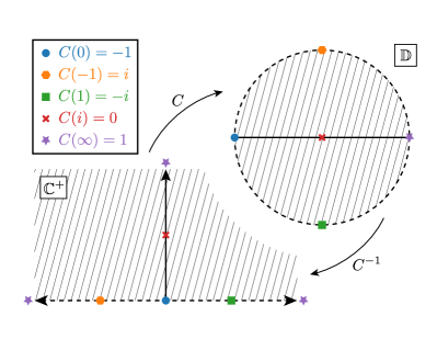
Figure 3: Diagramatic representation of the Cayley transform $C:\mathbb{C}^{+}\to\mathbb{D}$ and the inverse transform $C^{-1}:\mathbb{D}\to\mathbb{C}^{+}$. The real line is mapped to boundary of the unit disk, while the upper half-plane is mapped to its interior.

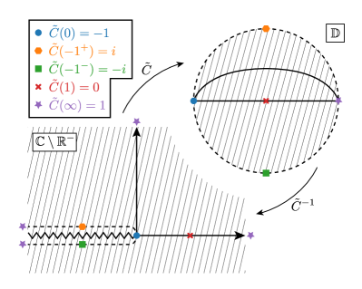
Figure 4: Diagrammatic representation of the transform $\widetilde{C}:\mathbb{C}\setminus R^{-}\to\mathbb{D}$ and the inverse transform $\widetilde{C}^{-1}:\mathbb{D}\to\mathbb{C}\setminus R^{-}$. The branch cut on the negative real line is mapped to the boundary of the unit disk. The positive real and imaginary axes are mapped to the indicated solid lines in the interior of the disk.

Since the bosonic spectral density is an odd function, $G_{-}$ is not a Nevanlinna function. Indeed, Eq. 20 shows that $\operatorname{Im}G_{-}$ is positive in the first quadrant and negative in the second quadrant. By symmetry, $\operatorname{Im}G_{-}$ only vanishes in the upper half plane along the positive imaginary axis, where the real part is strictly positive, $\operatorname{Re}G_{-}(iy)>0$ for $y>0$. In other words, $G_{-}:\mathbb{C}^{+}\to\mathbb{C}\setminus\mathbb{R}^{-}$, where $\mathbb{R}^{-}$ is the negative real line. This motivates defining a modified transform $\widetilde{C}:\mathbb{C}\setminus\mathbb{R}^{-}\to\mathbb{D}$ via

$$\widetilde{C}(z)=\frac{\sqrt{z}-1}{\sqrt{z}+1}, \widetilde{C}^{-1}(\zeta)=\left(\frac{1+\zeta}{1-\zeta}\right)^{2},$$ (34)

with the usual branch cut along the negative real line. The transformation $\tilde{C}$ is summarized visually in Fig. 4. Similar to the fermionic case, composition with $\widetilde{C}$ and the Cayley transorm then yields an associated function on the unit disk $\mathcal{G}_{-}:\mathbb{D}\to\mathbb{D}$:

$$\mathcal{G}_{-}(\zeta)=(\widetilde{C}\circ G_{R-}\circ C^{-1})(\zeta)$$ (35)

The functions $\mathcal{G}_{\pm}(\zeta)$ are members of the Schur class $\mathscr{S}$,

$$\mathscr{S}=\{f:\mathbb{D}\to\overline{\mathbb{D}}:f~{}\text{is analytic}\}.$$ (36)

The Schur class consists of non-constant analytic functions $f:\mathbb{D}\to\mathbb{D}$ as well as constant functions taking values in $\overline{\mathbb{D}}$. Viewed as elements of the Schur class, the functions $\mathcal{G}_{\pm}(\zeta)$ play a key role in the construction of interpolating functions below.

V Nevanlinna interpolation

The basic idea to constrain an analytic function starting from an interpolation problem in the complex plane dates back more than a century, to work from Pick [37] and Nevalinna [38, 39]. Most of the fundamental results needed for the present work were recently reviewed with modern terminology and notation in recent lectures by Nicolau [40], whose discussion we follow closely. Additional technical details and context are accessibly presented in Refs. [41, 42]. To keep the discussion self contained, we reproduce proofs for most of the necessary mathematical results. Although these results are well known to experts, we think it is valuable to collect them here with a consistent notation. The idea to use Nevanlinna interpolation for fermionic correlators was recently presented in Refs. [32, 33]. To our knowledge, Refs. [32, 33] were the first to apply the recursive approach to Nevanlinna interpolation, which we also follow, to problems in field theory.

V.1 An Interpolating Function on the Disk

In the preceding sections, we showed how the retarded Green functions $G_{\pm}(z)$ can be transformed into functions $\mathcal{G}_{\pm}(\zeta):\mathbb{D}\to\mathbb{D}$. We suppose that the Matsubara frequencies and Euclidean data have been mapped to the sets

$$\{i\omega_{\ell}\}\mapsto\{\zeta_{\ell}\}\subset\mathbb{D}$$ (37)

$$\{G_{\pm}(i\omega_{\ell})\}\mapsto\{w_{\ell}\}\subset\mathbb{D}$$ (38)

using Eqs. 32 and 34. Figure 5 summarizes the setup for the Matsubara frequencies, which are mapped to the interior of the unit disk. The task now is to construct a rational function $f(\zeta):\mathbb{D}\to\mathbb{D}$ which interpolates these points, i.e., satisfying $f(\zeta_{l})=w_{l}$. By construction, $f(\zeta)$ will be analytic on the unit disk and an element of the Hardy space $H^{\infty}$ (see, e.g., Ref. [43] for a discussion of Hardy spaces). To begin, it is useful to establish some notation. First, Blaschke factors are defined according to

$$b_{a}(\zeta)=\frac{|a|}{a}\frac{a-\zeta}{1-\bar{a}\zeta} a\in\mathbb{D}\setminus\{0\},$$ (39)

with $b_{0}(\zeta)\equiv\zeta=\mathrm{id}_{\mathbb{D}}$. Within particle physics, Blaschke factors play a familiar role in the conformal maps of the $z$-expansion used, for instance in the study of semileptonic decays of mesons [44, 45, 46, 47, 48, 49]. Blaschke factors enjoy several useful properties relevant for the present discussion. First, for $|a|<1$, Blaschke factors are automorphisms of the unit disk. Second, they clearly satisfy $b_{a}(a)$ = 0. Combining these properties with the maximum modulus principle means that any analytic function $g:\mathbb{D}\to\mathbb{D}$ with a zero at $a\in\mathbb{D}$ can be written in the factorized form $g(\zeta)=b_{a}(\zeta)\tilde{g}(\zeta)$ where $\tilde{g}(\zeta):\mathbb{D}\to\mathbb{D}$ is another analytic function [41, 42]. Finally, the following matrix notation for Möbius maps will prove very convenient,

$$\begin{pmatrix}a(\zeta)&b(\zeta)\\ c(\zeta)&d(\zeta)\end{pmatrix}h(\zeta)\equiv\frac{a(\zeta)h(\zeta)+b(\zeta)}{c(\zeta)h(\zeta)+d(\zeta)},$$ (40)

where $h(\zeta)$ is a function. One of the chief utilities of this notation is that function composition corresponds to matrix multiplication, with the matrix inverse coinciding to the function inverse.

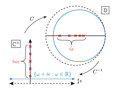
Figure 5: Mapping the Matsubara frequencies from the upper half-plane to the unit disk using the Cayley transform defined in Eq. 32. The blue line a distance $\epsilon$ above the real line is mapped to the blue circle in $\mathbb{D}$. We emphasize that the same mapping to the disk has been considered, for fermionic correlators, in Refs [32, 33] (cf. Fig 1 in Ref. [32]).

Let us now apply these ideas to the interpolation problem, proceeding by induction. For the base case, imposing $f(\zeta_{1})-w_{1}=0$ allows one to write

$$\frac{f(\zeta)-w_{1}}{1-\overline{w_{1}}f(\zeta)}=b_{\zeta_{1}}(\zeta)f_{1}(\zeta)$$ (41)

for some $f_{1}(\zeta)\in H^{\infty}$, since the left-hand side is an analytic function from the disk onto itself with zero at $w_{1}$. Solving for $f(\zeta)$ gives

$$f(\zeta) =\frac{b_{\zeta_{1}}(\zeta)f_{1}(\zeta)+w_{1}}{1+\overline{w_{1}}b_{\zeta_{1}}(\zeta)f_{1}(\zeta)}$$ (42)

$$=\frac{1}{\sqrt{1-|w_{1}|^{2}}}\begin{pmatrix}b_{\zeta_{1}}(\zeta)&w_{1}\\ \overline{w}_{1}b_{\zeta_{1}}(\zeta)&1\end{pmatrix}f_{1}(\zeta)$$ (43)

$$\equiv U_{1}(\zeta)f_{1}(\zeta),$$ (44)

where the normalization of the matrix $U_{1}(\zeta)$ has been chosen for later convenience so that $\det U_{1}(\zeta)=b_{\zeta_{1}}(\zeta)$. Imposing the interpolation condition $f(\zeta_{2})=w_{2}$ provides a constraint on the function $f_{1}(\zeta)$. Namely, Eq. 41 says that

$$f_{1}(\zeta_{2})=\frac{1}{b_{\zeta_{1}}(\zeta_{2})}\frac{w_{2}-w_{1}}{1-\overline{w}_{1}w_{2}}\equiv w_{2}^{(1)}$$ (45)

Thus, a Blaschke factor may be again be factored out to give

$$\frac{f_{1}(\zeta)-w_{2}^{(1)}}{1-\overline{w}_{2}^{(1)}f_{1}(\zeta)}=b_{z_{2}}(\zeta)f_{2}(\zeta),$$ (46)

in terms of some $f_{2}(\zeta)\in H^{\infty}$. Solving for $f_{1}(\zeta)$ then gives

$$f_{1}(\zeta)=\frac{b_{\zeta_{2}}(\zeta)f_{2}(\zeta)+w_{2}^{(1)}}{1+\overline{w}_{2}^{(1)}b_{\zeta_{2}}(\zeta)f_{2}(\zeta)}\equiv U_{2}(\zeta)f_{2}(\zeta),$$ (47)

with $U_{2}(\zeta)$ defined analogously to $U_{1}(\zeta)$. With this result, the inductive step now becomes obvious. Using all $N$ points,

$$f(\zeta) =U_{1}(\zeta)U_{2}(\zeta)\cdots U_{N}(\zeta)f_{N}(\zeta)$$ (48)

$$\equiv\begin{pmatrix}P_{N}(\zeta)&Q_{N}(\zeta)\\ R_{N}(\zeta)&S_{N}(\zeta)\\ \end{pmatrix}f_{N}(\zeta)$$ (49)

with $f_{N}(\zeta)\in H^{\infty}$. The functions $P_{N}$, $Q_{N}$, $R_{N}$, $S_{N}$ are call the Nevalinna coefficients. The matrices $U_{n}(\zeta)$ are defined according to

$$U_{n}(\zeta)=\frac{1}{\sqrt{1-\bigl{|}w_{n}^{(n-1)}\bigr{|}^{2}}}\begin{pmatrix}b_{\zeta_{n}}(\zeta)&w_{n}^{(n-1)}\\ \overline{w}_{n}^{(n-1)}b_{\zeta_{n}}(\zeta)&1\end{pmatrix}$$ (50)

where $w_{m}^{(n)}$ is the value of $f_{n}$ evaluated at the $m$th zero: $w_{m}^{(n)}\equiv f_{n}(\zeta_{m})$. An explicit formula for $w_{m}^{(n)}$ follows from imposing the interpolation condition

$$f(\zeta_{m}) =U_{1}(\zeta_{m})...U_{n}(\zeta_{m})w_{m}^{(n)}=w_{m}$$ (51)

$$w_{m}^{(n)} =U_{n}^{-1}(\zeta_{m})U_{n-1}^{-1}(\zeta_{m})\cdots U_{1}^{-1}(\zeta_{m})w_{m}$$ (52)

Since $f_{N}(\zeta)\in H^{\infty}$ is an arbitrary function, Eq. 49 actually parameterizes the full space of possible analytic continuations of the given finite data. Since freedom generically exists to include more points in the interpolation, the analytic continuation is not unique. Remarkably, the size of the solution space can quantified sharply.

To see this, consider space of solutions to the $N$-point interpolation problem evaluated at $\zeta$:

$$\Delta_{N}(\zeta)=\Bigl{\{}f(\zeta):f\in H^{\infty},f(\{\zeta_{n}\})=\{w_{n}\}\Bigr{\}}.$$ (53)

The size of this set determines the ambiguity in the analytic continuation at the point $\zeta$. For fixed $\zeta\in\overline{}\mathbb{D}$, the set can be written explicitly. The idea is to view Eq. 49 as a function of the undetermined $f_{N}(\zeta)\in\mathbb{D}$. From this viewpoint, it immediately follows that

$$\Delta_{N}(\zeta)=\{T_{N,\zeta}(w):w\in\mathbb{D}\},$$ (54)

where $T_{N,\zeta}:\mathbb{D}\to\mathbb{D}$ is the function

$$T_{N,\zeta}(w)=\frac{P_{N}(\zeta)w+Q_{N}(\zeta)}{R_{N}(\zeta)w+S_{N}(\zeta)}.$$ (55)

This parameterization makes it clear that $\Delta_{N}(\zeta)$ is a disk, since Möbius transformation map circles to circles. As proven in Appendix A, this function is into for all $|\zeta|<1$. Moreover, the function is onto when $|\zeta|=1$. We can also compute the center and radius of the disk $\Delta_{N}(\zeta)$. Since $T_{N,\zeta}(-S_{N}(\zeta)/R_{N}(\zeta))=\infty$, the reflection property of Möbius transformations implies that is $\Delta_{N}(\zeta)$ centered at

$$c_{N}(\zeta) =\frac{P_{N}(\zeta)\overline{(-R_{N}(\zeta)/S_{N}(\zeta))}+Q_{N}(\zeta)}{R_{N}(\zeta)\overline{(-R_{N}(\zeta)/S_{N}(\zeta))}+S_{N}(\zeta)}$$ (56)

$$=\frac{Q_{N}(\zeta)\overline{S}_{N}(\zeta)-P_{N}(\zeta)\overline{R}_{N}(\zeta)}{|S_{N}(\zeta)|^{2}-|R_{N}(\zeta)|^{2}}.$$ (57)

The radius of $\Delta_{N}(\zeta)$ can be computed by evaluating the distance between the center and its boundary. A brief calculation shows that the radius is given by

$$r_{N}(\zeta)=\frac{|B_{N}(\zeta)|}{|S_{N}(\zeta)|^{2}-|R_{N}(\zeta)|^{2}},$$ (58)

where $B_{N}(\zeta)=P_{N}(\zeta)S_{N}(\zeta)-Q_{N}(\zeta)R_{N}(\zeta)$. Collecting all the results, we see that $\Delta_{N}(\zeta)\subseteq\mathbb{D}$ is a disk of radius $r_{N}(\zeta)$ centered at $c_{N}(\zeta)$. Following the original work Nevanlinna [38, 39], this disk is sometimes known in the complex analysis literature as the Wertevorrat. The Wertevorrat $\Delta_{N}(\zeta)$ rigorously contains the full infinite family of all possible analytic continuations at each point $\zeta\in\mathbb{D}$.

V.2 The Pick Criterion

Given distinct $\zeta_{1},\zeta_{2},\dots,\zeta_{n}\in\mathbb{D}$ and any $w_{1},w_{2},\dots,w_{n}\in\mathbb{D}$, there exists a function in the Schur class $f\in\mathscr{S}$ which interpolates the points $f(\zeta_{i})=w_{i}$ for all $i$ if and only if the Pick matrix

$$\left[\frac{1-w_{i}\overline{w}_{j}}{1-\zeta_{i}\overline{\zeta}_{j}}\right]_{1\leq i,j\leq n}$$ (59)

is positive semidefinite  [40, 38, 39, 37, 41, 42]. If this criterion fails to hold, $f\notin\mathscr{S}$. For problems of physical interest, we expect the Pick criterion always to hold, at least if the Euclidean data are specified with sufficient precision. In practice, the Pick criterion may not be satisfied by noisy Monte Carlo data. This observation was also made in Refs. [32, 33]. In this case, the formal bounding guarantees may not hold. However, we expect the Wertevorrat will likely still provide quantitatively useful guidance. A promising idea is to apply a numerical “projection,” in the same spirit at SVD cuts or shrinkage in standard least-squares fitting, to restore the Pick criterion. Conceivably, this step could be done in such a way the “projection” data would be statistically consistent with the original data. Important work on robust spectral reconstructions in the presence of statistical noise has recently been given in Ref. [50].

V.3 Results Mapped to the Upper Half-plane

For physical interpretation, it now remains to translate the results of the preceding section back to the upper half-plane. The interpolating functions are readily mapped back by inverting Eqs. 33 and 35:

$$\begin{split}&G_{+}:\mathbb{C}^{+}\to\mathbb{C}^{+}\\ &G_{+}(z)=(C^{-1}\circ\mathcal{G}_{+}\circ C)(z)\end{split}$$ (60)

$$\begin{split}&G_{-}:\mathbb{C}^{+}\to\mathbb{C}\setminus\mathbb{R}^{-}\\ &G_{-}(z)=(\widetilde{C}^{-1}\circ\mathcal{G}_{-}\circ C)(z).\end{split}$$ (61)

Similarly, the Wertevorräte in the upper half-plane are given by

$$\mathcal{D}_{N}(z)\equiv\begin{cases}(C^{-1}\circ\Delta_{N}\circ C)(z)\text{ for }G_{+}\\ (\widetilde{C}^{-1}\circ\Delta_{N}\circ C)(z)\text{ for }G_{-}\end{cases}z\in\mathbb{C}^{+}.$$ (62)

Using the interpolating function, the smeared spectral density Eq. 28 can be computed via

$$\rho^{\epsilon}_{\pm}(\omega)=\frac{1}{\pi}\operatorname{Im}G_{\pm}(\omega+i\epsilon),$$ (63)

using the interpolating function for $G_{\pm}(z)$. Since $\Delta_{N}(\zeta)$ is an open set, so too is $\mathcal{D}_{N}(z)$, by invariance of domain. Let $\partial\mathcal{D}_{N}(z)$ denote its boundary. The uncertainty in the smeared spectral density is given by the full width of the imaginary part of the boundary of the Wertevorrat,

$$\begin{split}\delta\rho^{\epsilon}_{\pm}(\omega)=&\frac{1}{\pi}\left[\max\operatorname{Im}\partial\mathcal{D}_{N}(\omega+i\epsilon)\right.\\ &\left.-\min\operatorname{Im}\partial\mathcal{D}_{N}(\omega+i\epsilon)\right].\end{split}$$ (64)

The setup for $\rho^{\epsilon}_{\pm}(\omega)$ and $\delta\rho^{\epsilon}_{\pm}(\omega)$ is summarized in Fig. 6.

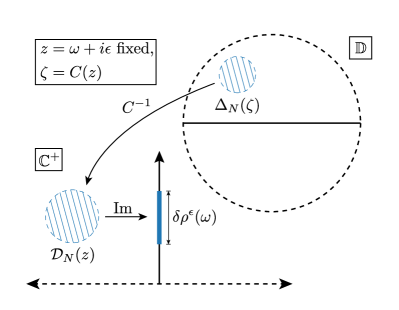
Figure 6: Mapping the Wertevorrat to $\mathbb{C}^{+}$ to evaluate the uncertainty in the smeared spectral density $\delta\rho^{\epsilon}(\omega)$.

Equation 64 has an appealing interpretation for $\epsilon=0$. As argued above, the Wertevorrat actually fills the full unit disk for boundary values:

$$|\zeta|=1\implies\Delta_{N}(\zeta)=\overline{\mathbb{D}}.$$ (65)

Since $C^{-1}(\overline{}\mathbb{D})=\overline{\mathbb{C}^{+}}$, the unsmeared spectral density is effectively unconstrained by the analytic continuation procedure:

$$\left.\delta\rho^{\epsilon}_{\pm}(\omega)\right|_{\epsilon=0}=\infty.$$ (66)

In other words, the ill-posed nature of unsmeared spectral reconstructions is manifest in the Wertevorrat formalism. However, given Euclidean data $G(i\omega_{l})$ at sufficiently many Matsubara frequencies, which amounts to large spatial volumes, $\rho^{\epsilon}_{\pm}(\omega)$ can be constrained tightly for $\epsilon>0$.

V.4 The Complete Algorithm

The method to compute smeared spectral densities $\rho^{\epsilon}(\omega)$ consists of the following steps:

1. Compute the Fourier coefficients $G_{E}^{(\ell)}$ via Eq. 14. These numbers constitute the Euclidean data.

2. Map Matsubara frequencies and Euclidean data to the unit disk using Eq. 32 and/or Eq. 34.

3. Solve the interpolation problem by computing the Nevanlinna coefficients and then compute the boundary of the Wertevorrat using Eq. 58.

4. Map the Wertevorrat from the disk back to the upper half-plane using Eq. 62.

5. Evaluate the space of smeared spectral densities using Eq. 64. The true smeared spectral function is rigorously bounded within this space.

Aside from incidental details, the algorithm is the same for both fermionic and bosonic quantities. Indeed, apart from the choice of conformal maps to transform the problem to the unit disk, all of the arguments from complex analysis are identical. Operationally, the two cases are distinguished by the choice of whether to compute Fourier coefficients using the bosonic or fermionic Matsubara frequencies in Item 1 above. This observation has a useful practical consequence.

Recall from Eq. 26 that, for a given set of energies and overlap factors, the zero-temperature spectral densities satisfy

$$\rho_{+}(\omega)=\operatorname{sgn}(\omega)\rho_{-}(\omega).$$ (67)

In particular, this implies that the smeared spectral densities converge to the same numerical result,

$$\lim_{\epsilon\to 0}\rho^{\epsilon}_{+}(\omega)=\operatorname{sgn}(\omega)\lim_{\epsilon\to 0}\rho^{\epsilon}_{-}(\omega).$$ (68)

In practice, this means that both the bosonic and fermionic methods define valid smeared spectral densities for zero-temperature Green functions in the sense of Eq. 8 as $\epsilon\to 0$. The choice of which one to use when analyzing zero-temperature data therefore becomes a question of convenience and expediency. In practice, it will likely prove useful to analyze both and construct the joint limit as $\epsilon$ approaches zero. A numerical example of this idea is given below.

Another way to see that $\rho^{\epsilon}_{\pm}(\omega)$ both define valid smeared spectral functions at zero temperature, in the sense of Eq. 8, is to note that experimental data can be smeared equally well to give $\rho^{\epsilon}_{+}(\omega)$ or $\rho^{\epsilon}_{-}(\omega)$, which can be compared to the result of spectral reconstruction.

With all the technical pieces now assembled, it is useful to highlight some similarities and important differences with recent work in the literature. The first difference has to do with the mapping of the Green functions to the unit disk. In Refs [32, 33], the insightful observation was made that fermionic Green functions have the Nevanlinna property ($\operatorname{Im}G_{+}(z)>0$ for all $z\in C^{+}$), which allowed the problem to be mapped to $\mathbb{D}$ with the Cayley transform in Eq. 32. The present treatment maps fermionic Green functions to the disk in precisely the same way. A new observation in the present work is that essentially the same idea holds for bosonic Green functions, provided the conformal map of Eq. 34 is used. In this sense, our perspective is that the Nevalinna property was a sufficient, but not necessary, condition to enable the use of the interpolation techniques for the unit disk in Ref. [32, 33] and Section V. Our treatment of bosonic Green functions differs from that of Ref. [34], where an auxiliary fermionic problem was constructed using the “hyperbolic tangent trick” [51, 11] to enable the use of the Cayley transform. The hyperbolic tanget trick appears to be related to the fluctuation dissipation theorem (cf. Eq. (39) in Ref. [35]) and holds in the unsmeared limit $\epsilon\to 0$. It would be interesting to explore its generalization to generic finite $\epsilon$ as well as the combination with error bounds from the Wertevorrat. Since fermionic spectral densities are positive for all $\omega\in\mathbb{R}$, reconstructions using the method of Ref. [34] may have attractive positivity features compared to the method in the present work.

A second important difference is related to how results are mapped back to the upper half-plane. Stated briefly, the algorithm in Refs. [32, 33, 34, 52] yields a single value for the smeared spectral function $\rho^{\epsilon}(\omega)$ for each $z=\omega+i\epsilon$ (essentially via Eq. 28), while the algorithm in the present work yields a bounding envelope via Eq. 64. In more detail, the difference stems from the following observations. As in Refs. [32, 33, 34, 52], the fundamental interpolation function on $\mathbb{D}$ is given by an equation like Eq. 49 which includes an undetermined function $f_{N}(\zeta)$ representing the freedom to include additional input data. In Refs. [32, 33, 34, 52], this freedom is exploited in a smoothing step, which removes spurious oscillations from the resulting spectral function. The smoothing step constrains the spectral function to minimize a certain convex functional enforcing the normalization sum rule ($\int d\omega\rho(\omega)=1$) and a notion of smoothness. To the best of our knowledge, no rigorous field-theoretic justification exists for the precise form of the smoothing criterion. The smoothed spectral functions certainly appear more physical and do seem to agree well with known results in numerical test cases given in Refs. [32, 33, 34, 52]. However, the perspective of the present work is that the smoothing step introduces an uncontrolled systematic uncertainty. For applications of interest in lattice QCD, this systematic uncertainty must be quantified. The present work takes a conservative stance, using the Wertevorrat [38, 39, 40] to characterize the full space of possible solutions. The Wertevorrat seems to have been long understood in the mathematical community. To the best of our knowledge, the present work is the first to recognize its role in bounding uncertainty in analytic continuation in field theory problems. It would be interesting to combine additional physical constraints (e.g. regarding the moments of the spectral functions as mentioned in Refs. [32, 33] and implemented in Ref. [52]) with the novel interpretation of the Wertevorrat.

VI Numerical calculation of $G(i\omega)$

A few words are in order about how to compute $G(i\omega_{l})$ given numerical data for $\mathscr{G}_{E}(\tau)$. As shown in Eq. 14, the desired frequency-space data are the Fourier coefficients of the Euclidean Green function. Since lattice QCD calculations provide Euclidean data for $\mathscr{G}_{E}(\tau)$ at the discrete times $\tau\in\{0,1,\dots\beta-1\}$, it is tempting to compute the Fourier coefficients with the discrete Fourier transform,

$$\int_{0}^{\beta}d\tau\,e^{i\omega_{\ell}\tau}\mathscr{G}_{E}(\tau) \stackrel{{\scriptstyle?}}{{\approx}}\sum_{t=0}^{\beta-1}e^{i\omega_{\ell}\tau}\mathscr{G}_{E}(\tau).$$ (69)

For the sake of illustration, let us carry out the bosonic Matsubara sum for a unit-amplitude Green function saturated by a single state, $\mathscr{G}_{E}(\tau)=e^{-m\tau}+e^{-m(\beta-\tau)}$. In this case, one readily finds

$$\sum_{\tau=0}^{\beta-1}e^{i\omega_{\ell}\tau}\mathscr{G}_{E}(\tau) =\frac{\left(1-e^{-\beta m}\right)\sinh(ma)}{\cosh(ma)-\cos(\omega_{l}a)},$$ (70)

where the implicit dependence on the lattice scale has been made explicit on the right-hand side. Trying to interpret the right-hand side as $G_{+}(i\omega_{l})$ is immediately problematic. Due to the periodicity of the denominator, the right-hand side is not analytic in the upper-half plane. Indeed, besides the expected pair of poles on the real axis, spurious poles also appear in the upper half-plane with offsets at $\pm ma+2\pi i\mathbb{Z}$. Nevertheless, the continuum limit has the correct analytic structure,

$$\lim_{a\to 0}a\frac{\left(1-e^{-\beta m}\right)\sinh(ma)}{\cosh(ma)-\cos(\omega_{l}a)}=\frac{2m}{m^{2}+\omega^{2}}.$$ (71)

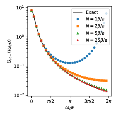
Figure 7: Numerical evaluation of the Fourier coefficients $G_{E}^{(\ell)}$ using different interpolation densities, using a Euclidean correlator $G_{E}(\tau)=e^{-m\tau}+e^{-m(\beta-\tau)}$ with $\beta=96$ and $m=0.25$. To avoid many overlapping points, results are shown for every third Matsubara frequency. The different markers show different interpolation refinements. The blue circles at the top are the result of the discrete Fourier transform of Eq. 70 and exhibit the expected pathology for large $\omega_{\ell}$. For an interpolation refinement of $25\beta/a$ (red stars), all Fourier coefficients agree with the exact continuum results with sub-percent precision.

This observation immediately suggests a solution, namely, constructing a better approximation to the integral of Eq. 14. Since $\mathscr{G}_{E}(t)$ is smooth and monotonic for $t\in\{0,\beta/2\}$, it can safely be interpolated, and this interpolation can be used to evaluate Eq. 14 numerically on a finer grid. In practice, it is advantageous to construct an interpolation of $\log\mathscr{G}_{E}(t)$, e.g., with a simple polynomial spline, since the logarithm is slowly varying. For example, Fig. 7 shows the result of this procedure for a range of grid refinements with $N\in\beta/a\times\{1,2,5,25\}$ total points. By interpolating, continuum-like values for $G_{\pm}(i\omega_{l})$ can be obtained, at least for low frequencies. For a given lattice spacing, estimating the high-frequency components ($\omega_{l}a\gg 1$) remains difficult from a practical perspective, since essentially all information about these components will have already decayed away by the first Euclidean time.

VII Numerical Examples

This section presents numerical examples of the algorithm described in Section V.4. In each case, the exact spectral density will specified. For simplicity, the zero-temperature limit will be used. It will be convenient to express the spectral density as a sum of arbitrarily close delta functions via Eq. 26. When the spectral density is evaluated numerically on a fine, uniform grid in energy with spacing $\Delta E$, the spectral weights are given by

$$|A_{0n}|^{2}=\int_{E_{n}}^{E_{n}+\Delta E}d\omega\,\rho(\omega),$$ (72)

where $E_{n}$ is the $n{\rm th}$ energy in the grid. The retarded Green function evaluated at the Matsubara frequencies then follows directly from Eq. 20. These values for $G_{E}^{(\ell)}=G_{\pm}(i\omega_{\ell})$ provide the starting data for the numerical examples.

VII.1 Discrete Spectral Features: Isolated Poles

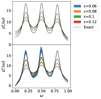
Figure 8: Smeared spectral reconstructions of spectral density with delta functions at $\omega\in\{0.2,0.5,0.8\}$ and with $\beta=64$. The upper (lower) panel shows fermionic (bosonic) reconstructions for several smearing widths. The dotted lines show the location of the exact result for each smearing width. The exact results lies within bounding envelope of the Wertevorrat.

Consider a Green function consisting of three isolated poles with masses $m\in\{0.2,0.5,0.8\}$ and unit residues. The corresponding spectral function on the positive real axis is

$$\rho(\omega)=\delta(\omega-0.2)+\delta(\omega-0.5)+\delta(\omega-0.8).$$ (73)

Using this spectral function as input, Euclidean data were generated along the imaginary-frequency axis at the Matsubara frequencies with $\beta=64$. The corresponding reconstructions are shown for a variety of smearing widths in Fig. 8. The upper (lower) panel shows the fermionic (bosonic) reconstruction. In all cases, the exact result lies within the rigorous bounding envelope of the Wertevorrat. In the fermionic case, the width of the bounding envelope is too small to see visibly.

VII.2 Extended Spectral Features: Gaussians

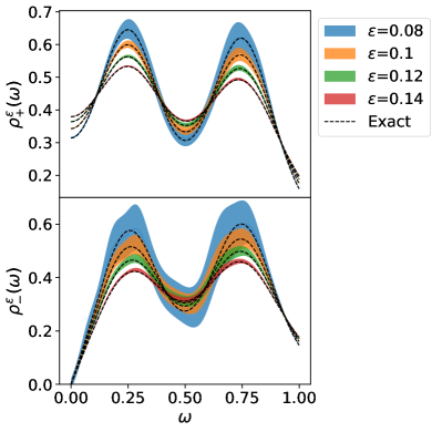
Figure 9: Smeared spectral reconstructions of a spectral densitity consisting of a pair of Gaussians, Eq. 74. Euclidean data were generated with $\beta=48$. The upper (lower) panel shows fermionic (bosonic) reconstruction for several smearing widths. The dotted lines shows the location of the exact result for each smearing width. In all cases, the exact result lies visibly within the bounding envelope of the Wertevorrat.

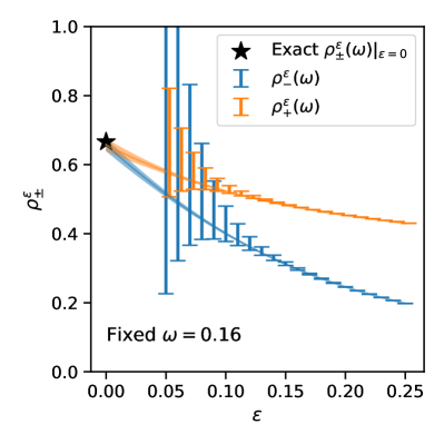
Figure 10: Example extrapolation to zero smearing width for the Gaussian example of Eq. 74 for fixed energy. The data points shows reconstructions for $\rho^{\epsilon}_{\pm}(\omega)$. The solid curve shows the result of a polynomial fit imposing Eq. 68. The black star shows the exact result from Eq. 74.

Consider a spectral function on the positive real axis consisting of a sum of Gaussians

$$\rho(\omega)=\sum_{i}\frac{1}{\sqrt{2\pi}\sigma_{i}}\exp\left(-\frac{(\omega-\mu_{i})^{2}}{2\sigma_{i}^{2}}\right),$$ (74)

where $\mu=\{0.25,0.75\}$ and $\sigma=\{0.1,0.1\}$. Using this spectral function as input, Euclidean data were generated along the imaginary-frequency axis at the Matsubara frequencies with $\beta=48$.

The corresponding reconstructions are shown for a variety of smearing widths in Fig. 9. The upper (lower) panel shows the fermionic (bosonic) reconstruction. In all cases, the exact result lies within the rigorous bounding envelope of the Wertevorrat. Figure 10 shows an example of how the bosonic and fermionic reconstruction may be used together to reconstruct their shared liming value of $\rho_{\pm}(\omega)$, cf. Eq. 68.

VII.3 The $R-$Ratio

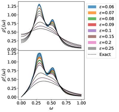
Figure 11: Smeared spectral reconstructions of a parameterization of experimental data for the R-ratio. Euclidean data were generated with $\beta/a=96$. The smearing choices $\epsilon$ are described in the main text. In both cases, the exact result lies visibly within the bounding envelope from the Wertevorrat. In both cases, the spectral peaks from the $\rho(770)/\omega(782)$ and from the $\phi(1020)$ are clearly visible.

A parameterization of the experimental data for $R(s)$ is given in Ref. [2] in terms of Breit-Wigner curves with masses, widths, and amplitudes chosen to match data in the PDG. The present example uses same parameterization and numerical input values as Ref. [2].

Numerical Euclidean data were generated using this parameterization as input for the spectral density with $\beta=96$. The energy range of the problem was rescaled to lie in the unit interval. This rescaling places the peak for the $\rho(770)$ at $\omega a\approx 0.25$, which amounts to a lattice spacing of $a\approx 0.07$ fm, a typical cutoff scale appearing in recent calculations of the anomalous magnetic moment of the muon [53, 54, 55, 56, 57, 58, 59, 60, 61, 62].

The corresponding reconstructions are shown for a variety of smearing widths in Fig. 11. The upper (lower) panel shows the fermionic (bosonic) reconstruction. The two peaks from the $\rho(770)/\omega(782)$ and the $\phi(1020)$ are clearly identified in both reconstructions. In all cases, the exact result lies within the rigorous bounding envelope of the Wertevorrat.

A reconstruction of $R(s)$ from lattice QCD data using the method of Ref. [8] was recently given in Ref. [63], where the authors also compared to experimental results including statistical uncertainties. We hope to conduct a similar test soon using the present method with correlation functions computed using lattice QCD as well as the actual experimental data.

VIII Conclusions

This work has presented a method for numerical analytic continuation, which is closely related to recent work in Refs. [32, 33, 34, 52]. The main application we have in mind is extracting spectral densities from Euclidean data (e.g., computing using lattice QCD). One of our main insights is that evaluating a Green function in the upper half-plane, Eq. 28, amounts to a smearing prescription in the spirit of Eq. 8. The general formalism is valid for generic (diagonal) thermal Green functions. As a proof of concept, we presented numerical examples of the method in a few simplified systems. Important work on robust spectral reconstructions in the presence of statistical noise has recently been given in Ref. [50].

A key distinguishing feature of our method from recent work in Refs. [32, 33, 34, 52] is the rigorous bounding envelope of the Wertevorrat, which quantifies the systematic uncertainty of the analytic continuation at each point $z$ in the upper half-plane. The Wertevorrat parameterizes, by explicit construction, the full space of functions consistent with input Euclidean data and with the known causal structure of Green’s function in the complex plane.

Another attractive feature of the method is the ease of including additional information, be it experimental or theoretical, to constrain the spectral reconstructions. For example, when calculating the inclusive structure functions in the resonance region, it might be desirable to constrain the behavior around the elastic scattering peak with lattice QCD data from simpler three-point correlation functions. Likewise, guidance from perturbation theory may usefully constrain and stabilize reconstructions at high energies. Regardless of precise source of the constraint, all that’s required is to translate the constraints to the upper-half plane and include them numerically in the interpolation problem. Moreover, the constraining data can be specified wherever it is known most precisely, including just above the real line and not necessarily on the imaginary-frequency axis. As with the general method itself, all constraints are included non-parametrically. Recent work has also explored the inclusion of constraints, especially moments of the spectral function [32, 33, 52].

Looking beyond applications in lattice QCD, the problem of computing inverse Laplace transforms arises in many fields. For instance, in nuclear theory, Green’s function Monte Carlo is often used to infer nuclear electroweak response functions from their Laplace transforms, the so-called Euclidean response functions. [64, 65] It would be interesting to explore the application of the ideas explored in this paper to other domains.

Appendix A Technical Material

Lemma 1.

Let $w,z\in\mathbb{C}$ with $\overline{w}z\neq 1$. If $|z|<1$ and $|w|<1$, then $|\frac{w-z}{1-\overline{w}z}|<1$. If $|z|=1$ or $|w|=1$, then $|\frac{w-z}{1-\overline{w}z}|=1$.

Proof.

The proof is by calculation. Take the polar decomposition $z=re^{i\varphi}$. Then

$$\left|\frac{w-z}{1-\overline{w}z}\right|=\left|\frac{we^{-i\varphi}-r}{1-\overline{we^{-i\varphi}}r}\right|,$$ (75)

so it suffices to take $z=r\in\mathbb{R}$. This amounts to determining when

$$\frac{w-r}{1-\overline{w}r}\frac{\overline{w}-r}{1-wr} \leq 1$$

$$\iff(w-r)(\overline{w}-r) \leq(1-wr)(1-\overline{w}r)$$

Taking $w=|w|e^{i\theta}$, the previous inequality reduces to

$$|w|^{2}+r^{2}\leq 1+|w|^{2}r^{2}.$$

The inequality is clearly satisfied when both $r<1$ and $|w|<1$. The equality holds when either $r=1$ or $|w|=1$. ∎

The preceding lemma has immediate consequences for the interpolation problem in Sec. V. For fixed $z\in\overline{\mathbb{D}}$, the map $U_{n,z}:\mathbb{D}\to\mathbb{D}$ defined by

$$U_{n,z}(w)=\frac{w_{n}^{(n-1)}+b_{z_{n}}(z)w}{1+\overline{w_{n}^{(n-1)}}b_{z_{n}}(z)w}$$ (76)

is clearly into. The lemma also shows that $|b_{z_{n}}(z)|=1$ when $|z|=1$. Therefore, when $|z|=1$, $U_{n,z}$ is actually onto, i.e., the image of $U_{n,z}$ is the full open disk. The composition properties of Möbius transformations show, by induction, that the same is true for Eq. 55.

References

- Aoyama et al. [2020] T. Aoyama et al., The anomalous magnetic moment of the muon in the Standard Model, Phys. Rept. 887, 1 (2020), arXiv:2006.04822 [hep-ph] .
- Bernecker and Meyer [2011] D. Bernecker and H. B. Meyer, Vector Correlators in Lattice QCD: Methods and applications, Eur. Phys. J. A 47, 148 (2011), arXiv:1107.4388 [hep-lat] .
- Davier et al. [2020] M. Davier, A. Hoecker, B. Malaescu, and Z. Zhang, A new evaluation of the hadronic vacuum polarisation contributions to the muon anomalous magnetic moment and to , Eur. Phys. J. C 80, 241 (2020), published under the terms of the Creative Commons CC-BY license, [Erratum: Eur.Phys.J.C 80, 410 (2020)], arXiv:1908.00921 [hep-ph] .
- Manohar [1992] A. V. Manohar, An Introduction to spin dependent deep inelastic scattering, in Lake Louise Winter Institute: Symmetry and Spin in the Standard Model (1992) arXiv:hep-ph/9204208 .
- Chesnokov et al. [2022] V. V. Chesnokov, A. A. Golubenko, B. S. Ishkhanov, and V. I. Mokeev, CLAS Database for Studies of the Structure of Hadrons in Electromagnetic Processes, Phys. Part. Nucl. 53, 184 (2022).
- Blin et al. [2021] A. N. H. Blin, W. Melnitchouk, V. I. Mokeev, V. D. Burkert, V. V. Chesnokov, A. Pilloni, and A. P. Szczepaniak, Resonant contributions to inclusive nucleon structure functions from exclusive meson electroproduction data, Phys. Rev. C 104, 025201 (2021), arXiv:2105.05834 [hep-ph] .
- Pijpers and Thompson [1992] F. Pijpers and M. Thompson, Faster formulations of the optimally localized averages method for helioseismic inversions, Astronomy and Astrophysics 262, L33 (1992).
- Hansen et al. [2019] M. Hansen, A. Lupo, and N. Tantalo, Extraction of spectral densities from lattice correlators, Phys. Rev. D 99, 094508 (2019), arXiv:1903.06476 [hep-lat] .
- Shinaoka et al. [2017] H. Shinaoka, J. Otsuki, M. Ohzeki, and K. Yoshimi, Compressing green’s function using intermediate representation between imaginary-time and real-frequency domains, Phys. Rev. B 96, 035147 (2017).
- Otsuki et al. [2017] J. Otsuki, M. Ohzeki, H. Shinaoka, and K. Yoshimi, Sparse modeling approach to analytical continuation of imaginary-time quantum monte carlo data, Phys. Rev. E 95, 061302 (2017).
- Itou and Nagai [2020] E. Itou and Y. Nagai, Sparse modeling approach to obtaining the shear viscosity from smeared correlation functions, JHEP 07, 007, arXiv:2004.02426 [hep-lat] .
- Otsuki et al. [2020] J. Otsuki, M. Ohzeki, H. Shinaoka, and K. Yoshimi, Sparse modeling in quantum many-body problems, Journal of the Physical Society of Japan 89, 012001 (2020), https://doi.org/10.7566/JPSJ.89.012001 .
- Li et al. [2020] J. Li, M. Wallerberger, N. Chikano, C.-N. Yeh, E. Gull, and H. Shinaoka, Sparse sampling approach to efficient ab initio calculations at finite temperature, Phys. Rev. B 101, 035144 (2020).
- Chikano et al. [2018] N. Chikano, J. Otsuki, and H. Shinaoka, Performance analysis of a physically constructed orthogonal representation of imaginary-time green’s function, Phys. Rev. B 98, 035104 (2018).
- Shi et al. [2023] S. Shi, L. Wang, and K. Zhou, Rethinking the ill-posedness of the spectral function reconstruction — Why is it fundamentally hard and how Artificial Neural Networks can help, Comput. Phys. Commun. 282, 108547 (2023), arXiv:2201.02564 [hep-ph] .
- Chen et al. [2021] S. Y. Chen, H. T. Ding, F. Y. Liu, G. Papp, and C. B. Yang, Machine learning spectral functions in lattice QCD, (2021), arXiv:2110.13521 [hep-lat] .
- Kades et al. [2020] L. Kades, J. M. Pawlowski, A. Rothkopf, M. Scherzer, J. M. Urban, S. J. Wetzel, N. Wink, and F. P. G. Ziegler, Spectral Reconstruction with Deep Neural Networks, Phys. Rev. D 102, 096001 (2020), arXiv:1905.04305 [physics.comp-ph] .
- Zhou et al. [2023] K. Zhou, L. Wang, L.-G. Pang, and S. Shi, Exploring QCD matter in extreme conditions with Machine Learning, (2023), arXiv:2303.15136 [hep-ph] .
- Lechien and Dudal [2022] T. Lechien and D. Dudal, Neural network approach to reconstructing spectral functions and complex poles of confined particles, SciPost Phys. 13, 097 (2022), arXiv:2203.03293 [hep-lat] .
- Wang et al. [2022] L. Wang, S. Shi, and K. Zhou, Reconstructing spectral functions via automatic differentiation, Phys. Rev. D 106, L051502 (2022), arXiv:2111.14760 [hep-ph] .
- Valentine and Sambridge [2019] A. P. Valentine and M. Sambridge, Gaussian process models—I. A framework for probabilistic continuous inverse theory, Geophysical Journal International 220, 1632 (2019).
- Del Debbio et al. [2022] L. Del Debbio, T. Giani, and M. Wilson, Bayesian approach to inverse problems: an application to NNPDF closure testing, Eur. Phys. J. C 82, 330 (2022), arXiv:2111.05787 [hep-ph] .
- Candido et al. [2023] A. Candido, L. Del Debbio, T. Giani, and G. Petrillo, Inverse Problems in PDF determinations, PoS LATTICE2022, 098 (2023), arXiv:2302.14731 [hep-lat] .
- Horak et al. [2022] J. Horak, J. M. Pawlowski, J. Rodríguez-Quintero, J. Turnwald, J. M. Urban, N. Wink, and S. Zafeiropoulos, Reconstructing QCD spectral functions with Gaussian processes, Phys. Rev. D 105, 036014 (2022), arXiv:2107.13464 [hep-ph] .
- Pawlowski et al. [2022] J. M. Pawlowski, C. S. Schneider, J. Turnwald, J. M. Urban, and N. Wink, Yang-Mills glueball masses from spectral reconstruction, (2022), arXiv:2212.01113 [hep-ph] .
- Horak et al. [2023] J. Horak, J. M. Pawlowski, J. Turnwald, J. M. Urban, N. Wink, and S. Zafeiropoulos, Nonperturbative strong coupling at timelike momenta, Phys. Rev. D 107, 076019 (2023), arXiv:2301.07785 [hep-ph] .
- Rothkopf [2022a] A. Rothkopf, Inverse problems, real-time dynamics and lattice simulations, EPJ Web Conf. 274, 01004 (2022a), arXiv:2211.10680 [hep-lat] .
- Rothkopf [2022b] A. Rothkopf, Bayesian inference of real-time dynamics from lattice QCD, (2022b), arXiv:2208.13590 [hep-lat] .
- Bulava [2023] J. Bulava, The spectral reconstruction of inclusive rates, PoS LATTICE2022, 231 (2023), arXiv:2301.04072 [hep-lat] .
- Hansen et al. [2017] M. T. Hansen, H. B. Meyer, and D. Robaina, From deep inelastic scattering to heavy-flavor semileptonic decays: Total rates into multihadron final states from lattice QCD, Phys. Rev. D 96, 094513 (2017), arXiv:1704.08993 [hep-lat] .
- Bulava and Hansen [2019] J. Bulava and M. T. Hansen, Scattering amplitudes from finite-volume spectral functions, Phys. Rev. D 100, 034521 (2019), arXiv:1903.11735 [hep-lat] .
- Fei et al. [2021a] J. Fei, C.-N. Yeh, and E. Gull, Nevanlinna analytical continuation, Phys. Rev. Lett. 126, 056402 (2021a).
- Fei et al. [2021b] J. Fei, C.-N. Yeh, D. Zgid, and E. Gull, Analytical continuation of matrix-valued functions: Carathéodory formalism, Phys. Rev. B 104, 165111 (2021b).
- Nogaki and Shinaoka [2023] K. Nogaki and H. Shinaoka, Bosonic Nevanlinna Analytic Continuation, J. Phys. Soc. Jap. 92, 035001 (2023), arXiv:2305.03449 [quant-ph] .
- Meyer [2011] H. B. Meyer, Transport Properties of the Quark-Gluon Plasma: A Lattice QCD Perspective, Eur. Phys. J. A 47, 86 (2011), arXiv:1104.3708 [hep-lat] .
- Poggio et al. [1976] E. C. Poggio, H. R. Quinn, and S. Weinberg, Smearing the Quark Model, Phys. Rev. D 13, 1958 (1976).
- Pick [1915] G. Pick, Über die Beschränkungen analytischer Funktionen, welche durch vorgegebene Funktionswerte bewirkt werden, Math. Ann. 77, 7 (1915).
- Nevanlinna [1919] R. Nevanlinna, Über beschränkte Funktionen die in gegebenen punkten vorgeschriebene Werte annehmen, Ann. Acad. Sci. Fenn. Ser. A 13 (1919).
- Nevanlinna [1929] R. Nevanlinna, Über beschränkte analytische Funktionen, Ann. Acad. Sci. Fenn. Ser. A 32 (1929).
- Nicolau [2016] A. Nicolau, The Nevanlinna-Pick Interpolation Problem, in Proceedings of the Summer School in Complex and Harmonic analysis, and related topics, 22, edited by J. Gröhn, J. Heittokangas, R. Korhonen, and J. Rättyä (Publications of the University of eastern Finland, 2016) https://mat.uab.cat/artur/data/nevanlinna-pick.pdf.
- Garcia et al. [2018] S. Garcia, J. Mashreghi, and W. Ross, Finite Blashke Products and Their Connections, 1st ed. (Springer, 2018).
- Agler and McCarthy [2002] J. Agler and J. McCarthy, Pick Interpolation and Hilbert Function Spaces (American Mathematical Society, 2002).
- Nikolski [2019] N. Nikolski, Hardy Spaces, edited by D. Gibbons and G. Gibbons, Cambridge Studies in Advanced Mathematics (Cambridge University Press, 2019).
- Caprini et al. [1998] I. Caprini, L. Lellouch, and M. Neubert, Dispersive bounds on the shape of form-factors, Nucl. Phys. B 530, 153 (1998), arXiv:hep-ph/9712417 .
- Boyd et al. [1995a] C. G. Boyd, B. Grinstein, and R. F. Lebed, Constraints on form-factors for exclusive semileptonic heavy to light meson decays, Phys. Rev. Lett. 74, 4603 (1995a), arXiv:hep-ph/9412324 .
- Boyd et al. [1995b] C. G. Boyd, B. Grinstein, and R. F. Lebed, Model independent extraction of using dispersion relations, Phys. Lett. B 353, 306 (1995b), arXiv:hep-ph/9504235 .
- Boyd et al. [1996] C. G. Boyd, B. Grinstein, and R. F. Lebed, Model independent determinations of , form factors, Nucl. Phys. B 461, 493 (1996), arXiv:hep-ph/9508211 .
- Boyd et al. [1997] C. G. Boyd, B. Grinstein, and R. F. Lebed, Precision corrections to dispersive bounds on form-factors, Phys. Rev. D 56, 6895 (1997), arXiv:hep-ph/9705252 .
- Grinstein and Kobach [2017] B. Grinstein and A. Kobach, Model-Independent Extraction of from , Phys. Lett. B 771, 359 (2017), arXiv:1703.08170 [hep-ph] .
- Huang et al. [2023] Z. Huang, E. Gull, and L. Lin, Robust analytic continuation of Green’s functions via projection, pole estimation, and semidefinite relaxation, Phys. Rev. B 107, 075151 (2023), arXiv:2210.04187 [cond-mat.str-el] .
- Meyer [2007] H. B. Meyer, A Calculation of the shear viscosity in SU(3) gluodynamics, Phys. Rev. D 76, 101701 (2007), arXiv:0704.1801 [hep-lat] .
- Nogaki et al. [2023] K. Nogaki, J. Fei, E. Gull, and H. Shinaoka, Nevanlinna.jl: A julia implementation of nevanlinna analytic continuation (2023), arXiv:2302.10476 [physics.comp-ph] .
- Borsanyi et al. [2021] S. Borsanyi et al., Leading hadronic contribution to the muon magnetic moment from lattice QCD, Nature 593, 51 (2021), arXiv:2002.12347 [hep-lat] .
- Chakraborty et al. [2018] B. Chakraborty et al. (Fermilab Lattice, LATTICE-HPQCD, MILC), Strong-Isospin-Breaking Correction to the Muon Anomalous Magnetic Moment from Lattice QCD at the Physical Point, Phys. Rev. Lett. 120, 152001 (2018), arXiv:1710.11212 [hep-lat] .
- Borsanyi et al. [2018] S. Borsanyi et al. (Budapest-Marseille-Wuppertal), Hadronic vacuum polarization contribution to the anomalous magnetic moments of leptons from first principles, Phys. Rev. Lett. 121, 022002 (2018), arXiv:1711.04980 [hep-lat] .
- Blum et al. [2018] T. Blum, P. A. Boyle, V. Gülpers, T. Izubuchi, L. Jin, C. Jung, A. Jüttner, C. Lehner, A. Portelli, and J. T. Tsang (RBC, UKQCD), Calculation of the hadronic vacuum polarization contribution to the muon anomalous magnetic moment, Phys. Rev. Lett. 121, 022003 (2018), arXiv:1801.07224 [hep-lat] .
- Giusti et al. [2019] D. Giusti, V. Lubicz, G. Martinelli, F. Sanfilippo, and S. Simula (ETM), Electromagnetic and strong isospin-breaking corrections to the muon from Lattice QCD+QED, Phys. Rev. D99, 114502 (2019), arXiv:1901.10462 [hep-lat] .
- Shintani and Kuramashi [2019] E. Shintani and Y. Kuramashi, Study of systematic uncertainties in hadronic vacuum polarization contribution to muon with 2+1 flavor lattice QCD, Phys. Rev. D100, 034517 (2019), arXiv:1902.00885 [hep-lat] .
- Davies et al. [2020] C. T. H. Davies et al. (Fermilab Lattice, LATTICE-HPQCD, MILC), Hadronic-vacuum-polarization contribution to the muon’s anomalous magnetic moment from four-flavor lattice QCD, Phys. Rev. D101, 034512 (2020), arXiv:1902.04223 [hep-lat] .
- Gérardin et al. [2019] A. Gérardin, M. Cè, G. von Hippel, B. Hörz, H. B. Meyer, D. Mohler, K. Ottnad, J. Wilhelm, and H. Wittig, The leading hadronic contribution to from lattice QCD with flavours of O() improved Wilson quarks, Phys. Rev. D100, 014510 (2019), arXiv:1904.03120 [hep-lat] .
- Aubin et al. [2020] C. Aubin, T. Blum, C. Tu, M. Golterman, C. Jung, and S. Peris, Light quark vacuum polarization at the physical point and contribution to the muon , Phys. Rev. D101, 014503 (2020), arXiv:1905.09307 [hep-lat] .
- Giusti and Simula [2019] D. Giusti and S. Simula, Lepton anomalous magnetic moments in Lattice QCD+QED, PoS LATTICE2019, 104 (2019), arXiv:1910.03874 [hep-lat] .
- Alexandrou et al. [2022] C. Alexandrou et al., Probing the -ratio on the lattice, (2022), arXiv:2212.08467 [hep-lat] .
- Carlson et al. [2015] J. Carlson, S. Gandolfi, F. Pederiva, S. C. Pieper, R. Schiavilla, K. E. Schmidt, and R. B. Wiringa, Quantum Monte Carlo methods for nuclear physics, Rev. Mod. Phys. 87, 1067 (2015), arXiv:1412.3081 [nucl-th] .
- King et al. [2020] G. B. King, L. Andreoli, S. Pastore, M. Piarulli, R. Schiavilla, R. B. Wiringa, J. Carlson, and S. Gandolfi, Chiral Effective Field Theory Calculations of Weak Transitions in Light Nuclei, Phys. Rev. C 102, 025501 (2020), arXiv:2004.05263 [nucl-th] .