Martian time-series unraveled:
A multi-scale nested approach with factorial variational autoencoders

Abstract

Unsupervised source separation involves unraveling an unknown set of source signals recorded through a mixing operator, with limited prior knowledge about the sources, and only access to a dataset of signal mixtures. This problem is inherently ill-posed and is further challenged by the variety of time-scales exhibited by sources in time series data from planetary space missions. As such, a systematic multi-scale unsupervised approach is needed to identify and separate sources at different time-scales. Existing methods typically rely on a preselected window size that determines their operating time-scale, limiting their capacity to handle multi-scale sources. To address this issue, instead of directly operating in the time domain, we propose an unsupervised multi-scale clustering and source separation framework by leveraging wavelet scattering covariances that provide a low-dimensional representation of stochastic processes, capable of effectively distinguishing between different non-Gaussian stochastic processes. Nested within this representation space, we develop a factorial Gaussian-mixture variational autoencoder that is trained to (1) probabilistically cluster sources at different time-scales and (2) independently sample scattering covariance representations associated with each cluster. As the final stage, using samples from each cluster as prior information, we formulate source separation as an optimization problem in the wavelet scattering covariance representation space, resulting in separated sources in the time domain. When applied to seismic data recorded during the NASA InSight mission on Mars, containing sources varying greatly in time-scale, our multi-scale nested approach proves to be a powerful tool for discriminating between such different sources, e.g., minute-long transient one-sided pulses (known as “glitches”) and structured ambient noises resulting from atmospheric activities that typically last for tens of minutes. These results provide an opportunity to conduct further investigations into the isolated sources related to atmospheric-surface interactions, thermal relaxations, and other complex phenomena.

1 Introduction

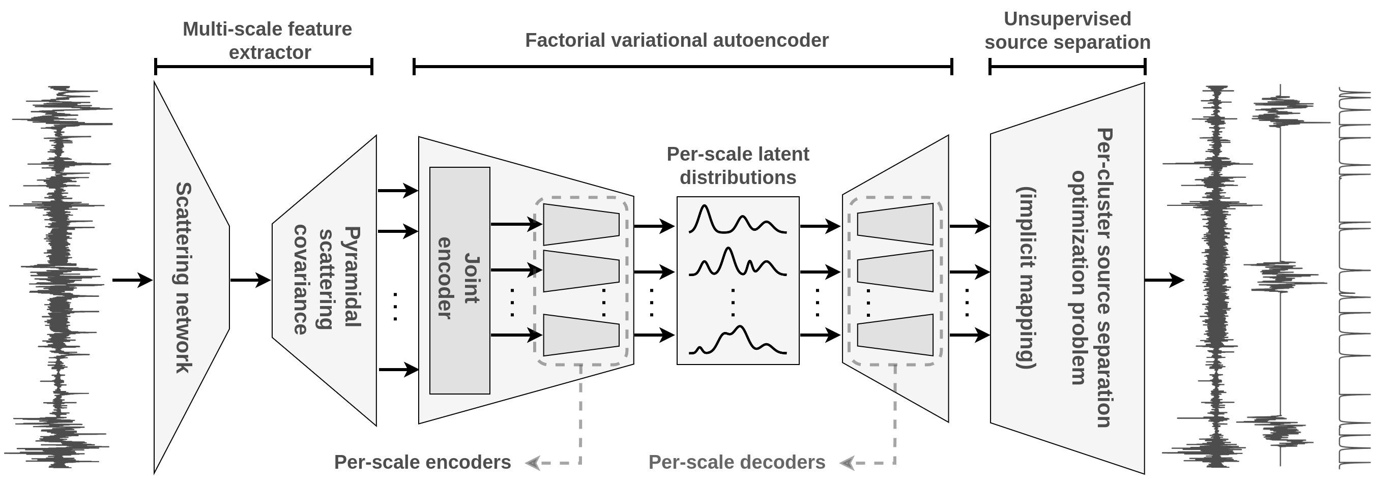
Figure 1: A schematic diagram depicting the proposed unsupervised multi-scale clustering and source separation framework. In the factorial variational autoencoder schematic, multiple arrows going from one block to another indicate representations associated with different time-scales.

Source separation is a challenging and often ill-posed problem that involves retrieving an a priori unknown number of sources from given time-series in which only their mixture is observed. Typically, there is limited prior knowledge available about each source, leading to an underdetermined problem. While certain domains may benefit from prior information, such as certain assumptions about source regularity, this is not always the case, particularly when dealing with data obtained from extraterrestrial missions. In such scenarios, it is highly uncertain how to acquire reliable expert knowledge for interpreting the recorded data. Nevertheless, the ability to perform source separation is crucial in advancing our understanding of the recorded events. While classical source separation methods [1, 2, 3, 4, 5, 6] have been extensively studied and are well understood, they often rely on simplifying assumptions about the sources. These assumptions, if not realistic, can introduce bias into the outcome of the source separation process [5, 7]. In contrast, supervised source separation methods [8, 9, 10, 11, 12] aim to separate sources by utilizing labeled training data, comprising pairs of sources and their mixtures. However, in domains with limited expert knowledge, obtaining such training data is often challenging, making supervised learning methods unsuitable. Furthermore, the use of synthetic data to artificially generate labels also proves challenging when the signal to be generated is not thoroughly understood.

In light of the limited availability of prior knowledge about sources and the sole access to a dataset of mixed signals, a truly unsupervised source separation method is needed. While existing unsupervised source separation methods have demonstrated success, they are not well-suited to handle sources with vastly varying time-scales as they typically rely on preselected window sizes, limiting them to sources that are detectable within the time-scale of the window. While existing unsupervised source separation methods have demonstrated success [13, 14, 15, 16, 17, 18], they are not well-suited to handle sources with vastly varying time-scales due their reliance on preselected window sizes. This limits their usage to separating sources that span within the window’s time-scale. This limitation can be a critical obstacle in analyzing complex phenomena that involve sources with vastly different time-scales. Thus, there is a pressing need to develop a new method that can overcome this limitation and provide a multi-scale unsupervised approach for source separation.

To address this problem, we present an unsupervised multi-scale clustering and source separation framework that is capable of detecting and separating prominent sources in a dataset of signal mixtures. To systematically incorporate the multi-scale nature of the data into our design, we develop the framework within the wavelet scattering covariance representation space [19]. These are correlation features on the output of a scattering network [20], which captures the non-Gaussian and multi-scale characteristics of stochastic processes in the data. Exploiting this representation space, we develop our method in three steps (see Figure 1 for a schematic diagram),

• We calculate the wavelet scattering covariance representation at different time-scales, resulting in a double multi-scale description of the data that extends wavelet scattering covariances to non-stationary processes (first contribution);

• Using this representation, we introduce a factorial variant of Gaussian-mixture variational autoencoders [VAEs; 21, 22, 23] (second contribution), hereon referred to as fVAE, that simultaneously learns to probabilistically cluster sources at different time-scales in the latent space and independently sample scattering covariance representations associated with each cluster. The former provides clusters of prominent sources in the dataset at different time-scales, and the latter models the wavelet scattering covariance distribution of these sources, providing prior information necessary for source separation;

• Finally, we perform source separation by complementing the method proposed by Siahkoohi et al. [24] by the learned prior information regarding each source (third contribution). Our method for source separation involves solving an optimization problem over the unknown sources in the wavelet scattering covariance representations space. This is achieved by minimizing carefully selected and normalized loss functions that incorporate prior knowledge about the source of interest, ensure data-fidelity, and impose statistical independence between the recovered sources.

The proposed strategy is able to perform source separation in the scattering space known to be stable to spurious deformation, while enabling sampling of the separate sources, a must for interpretability and knowledge discovery. We, however, do not consider inverting for the mixing operator and simply consider an identity forward model. To illustrate the ability of our approach to handle very complex time-series, we apply it to seismic data recorded during NASA’s Interior Exploration using Seismic Investigations, Geodesy and Heat Transport (InSight) mission [25, 26, 27]. This dataset provides valuable information to study of the Red Planet’s interior structure and composition [28], however, the recorded signal is heavily influenced by atmospheric activity and surface temperature [29, 30], leading to a distinct daily pattern and a pronounced non-stochastic character.

In the following sections, we provide an overview of relevant unsupervised source separation techniques. We then introduce the utilization of wavelet scattering covariance as a representation rich in domain knowledge for analyzing multi-scale time series. Furthermore, we explain how we extend this representation to handle non-stationary processes. The core of our approach lies in the description of factorial Gaussian-mixture VAEs, which enable multi-scale clustering and sampling of scattering covariances. These can be used as prior information for source separation. In the final stage of our framework, we detail our source separation approach, which involves solving an optimization problem using loss functions defined in the wavelet scattering covariance space. Lastly, we present the results of applying our approach to the seismic dataset obtained from the InSight mission.

2 Related work

In the context of unsupervised source separation methods, in a comprehensive study, Delouis, J.-M. et al. [31] proposes an optimization-based source separation technique using non-linear wavelet covariance representations on full sky observations of dust emission. Our proposed fVAE, along with the learned prior, can complement this method by offering a probabilistic and systematic way to select noise realizations. Our fVAE can also be used to embed prior knowledge into the Bayesian framework introduced by Jeffrey et al. [32]. This framework utilizes a scattering transform generative model for source separation and assumes training samples from each source. None of the above methods explicitly address the challenges of non-stationary data with sources at multiple time-scales. To tackle this issue, a supervised approach proposed by Stoller et al. [33] utilizes an auto-regressive model to capture long-distance relationships in the input audio. However, this approach solely relies on time-domain data and does not leverage the valuable domain knowledge available in signal and time-series processing, which could enhance source separation.  Denton et al. [17] performs unsupervised sources separation with the aim to improve bird sound classification. While the underlying source separation method is unsupervised [15], it is unclear how it handles sources with vastly different time-scales as not explicit multi-scale structure is expoited.

3 Non-stationary scattering covariance representation

Time-series data $\mathbf{x}$ recorded during space missions is often considered as non-stationary non-Gaussian noise and is multi-scale in a double meaning. The signal $\mathbf{x}$ has variations on a wide range of scales (noisy signal), second, different sources have generally different time-scales, some of them happening at the scale of the minute, others happening at the scale of the day, which contributes to non-stationarity. This section builds a representation adapted to this doubly multi-scale aspect of data by introducing non-stationary wavelet scattering covariance which are multi-scale averages on correlation features on a two-layer convolutional neural network with predefined wavelet filters.

3.1 Wavelet scattering networks

A scattering network [20] is a cascade of wavelet operators $\mathbf{W}$ followed by nonlinear activation function (akin to a typical convolutional neural network). A wavelet transform $\mathbf{W}$ is a convolutional operator with predefined wavelet filters that extracts variations at separate scales. These filters include a low-pass filter $\varphi_{J}(t)$ and $J$ complex-valued band-pass filters $\psi_{j}(t)=2^{-j}\psi(2^{-j}t),\ 1\leq j\leq J$, which are obtained by the dilation of a mother wavelet $\psi(t)$ and have zero-mean and a fast decay away from $t=0$. The wavelet coefficient $\mathbf{W}\mathbf{x}=x\star\psi_{j}(t)$ extracts variations of the input signal $\mathbf{x}(t)$ around time $t$ at scale $2^{j}$. In order to capture non-linear variations such as envelope modulation, we use a modulus activation function $|\cdot|$ and cascade a second wavelet operator. The output of a two-layer scattering network $S$ is $S(\mathbf{x}):=\big{(}\mathbf{W}\mathbf{x}\,,\,\mathbf{W}|\mathbf{W}\mathbf{x}|\big{)}^{\top}$, and it extracts variations of signal $\mathbf{x}$ and its multi-scale envelopes $|\mathbf{W}\mathbf{x}|$ at different times and different scales. Even though these networks have many successful applications e.g. intermittency analysis [34], clustering [35], event detection and segmentation [36] (with learnable wavelets), these are not sufficient to build accurate description of a multiscale process as they do not capture crucial dependencies across different scales [19].

3.2 Capturing non-Gaussian characteristics of random processes

Sources $\mathbf{x}$ encountered in time-series studied in this paper can be considered as strongly non-Gaussian processes. For sake of simplicity, let us assume $\mathbf{x}$ is a stationary source. If $\mathbf{x}$ were Gaussian then the different scale channels of a scattering networks would be independent, however it is not the case in practice and these dependencies were shown to be crucial to characterize the non-Gaussian stochastic structure of $\mathbf{x}$ [19]. Such dependencies can be captured by considering the correlation matrix ${\mathbb{E}}\{S(\mathbf{x})S(\mathbf{x})^{\top}\}$

$${\mathbb{E}}\begin{bmatrix}\mathbf{W}\mathbf{x}\left(\mathbf{W}\mathbf{x}\right)^{\top}&\mathbf{W}\mathbf{x}\left(\mathbf{W}|\mathbf{W}\mathbf{x}|\right)^{\top}\\ \mathbf{W}|\mathbf{W}\mathbf{x}|\left(\mathbf{W}\mathbf{x}\right)^{\top}&\mathbf{W}|\mathbf{W}\mathbf{x}|\left(\mathbf{W}|\mathbf{W}\mathbf{x}|\right)^{\top}\end{bmatrix}.$$ (1)

This matrix contains three types of coefficients. Correlation coefficients ${\mathbb{E}}\{\mathbf{W}\mathbf{x}\left(\mathbf{W}\mathbf{x}\right)^{\top}\}$ come down to the wavelet power spectrum, which characterizes in particular the roughness of the signal. Correlation coefficients ${\mathbb{E}}\{\mathbf{W}\mathbf{x}\left(\mathbf{W}|\mathbf{W}\mathbf{x}|\right)^{\top}\}$ capture signed interaction between wavelet coefficients. In particular, they detect sign-asymmetry and time-asymmetry in $\mathbf{x}$ [19]. Finally, coefficients ${\mathbb{E}}\{\mathbf{W}|\mathbf{W}\mathbf{x}|\left(\mathbf{W}|\mathbf{W}\mathbf{x}|\right)^{\top}\}$ capture correlations between signal envelopes $|\mathbf{W}\mathbf{x}|$ at different scales. These correlations account for intermittency and time-asymmetry [19].

Owing to the compression properties of wavelet operators [37] for the type of signals considered in this paper, these matrices are quasi-diagonal. We denote ${\mathbb{E}}\{\operatorname{diag}\left(S(\mathbf{x})S(\mathbf{x})^{\top}\right)\}$ an appropriate diagonal approximation of the full sparse matrix (13). The expectation ${\mathbb{E}}$ is replaced by a time average denoted by $\underset{}{\operatorname{Ave}}\,$ (average pooling) whose size should be chosen as the typical duration of event $\mathbf{x}$. The wavelet scattering covariance representation is

$$\Psi(\mathbf{x}):=\underset{}{\operatorname{Ave}}\,\big{(}S(\mathbf{x})\,,\,\operatorname{diag}\left(S(\mathbf{x})S(\mathbf{x})^{\top}\right)\big{)}.$$ (2)

It extracts average and correlation features from a 2-layer convolutional neural network with predefined wavelet filters. It is analogous to the features extracted in Gatys et al. [38] for generation. However, we do not train any weights in our representation. Owing to the compression properties of wavelet operators we obtain a low-dimensional representation. For a signal $\mathbf{x}\in\mbox{$\mathbb{R}$}^{L}$ of length $L$ the scattering covariance is smaller than $\log^{3}_{2}(L)$ (at least for $L\geq 3$) [19]. As a consequence, our representation that contains only order 1 and order 2 statistics has a low-variance which will be crucial for clustering.

3.3 Pyramidal scattering covariance features

Non-stationarity in the data is in part explained by the presence of sources with different time durations. Consider a signal $\mathbf{x}$ that is a superposition of sources with different time-durations. Our representation $\Psi(\mathbf{x})$ averages scattering covariance features on a certain window. If a source $\mathbf{s}$ has a time-duration that is much smaller than the average window size then it will be averaged out and the representation will barely feature information about such source. To take into account the variety of source durations, we consider different averaging sizes in a causal manner. We replace $\underset{}{\operatorname{Ave}}\,{}$ in (2) by a multi-scale average pooling operator $\underset{}{\operatorname{Ave}}\,=\big{(}\underset{t\in w_{1}}{\operatorname{Ave}}\,\,,\,\ldots\,,\,\underset{t\in w_{K}}{\operatorname{Ave}}\,\big{)}$. Windows $w_{1},\ldots,w_{K}$ have a pyramidal structure, they are of increasing size, all ending at same time, $\underset{t\in w_{1}}{\operatorname{Ave}}\,$ looks at recent past while $\underset{t\in w_{K}}{\operatorname{Ave}}\,$ looks at distant past. To cover a large range of time-scales with few factors we choose $w_{k+1}$ to be four times longer than $w_{k}$. This defines a pyramidal scattering covariance representation $\Psi(x)=(\Psi_{1}(x),\ldots,\Psi_{K}(x))$ whose factor $k$ is

$$\Psi_{k}(\mathbf{x}):=\underset{t\in w_{k}}{\operatorname{Ave}}\,\big{(}S(\mathbf{x})\,,\,\operatorname{diag}\left(S(\mathbf{x})S(\mathbf{x})^{\top}\right)\big{)}.$$ (3)

Representation $\Psi(\mathbf{x})$ decomposes the variation over time in the stochastic structure of process $\mathbf{x}$ (seen through scattering covariance) at multiple scales through a multi-scale operator $\underset{}{\operatorname{Ave}}\,$. To our knowledge it is the first scattering-like representation that tackles non-stationary processes.

4 Factorial Gaussian-mixture variational autoencoder (fVAE)

To efficiently perform source separation on our multi-scale representation, we require a generative model that can simultaneously cluster and sample. As Gaussian-mixture VAEs [21, 22, 23] are capable of learning highly structured, low-dimensional latent representations of data, they are a promising candidate for achieving our goals. The major open question remains on the structure of the mapping between the input space time-series and latent space cluster variables. As our aim is to cluster — or separate — sources co-occurring with different time-scales, we propose a factorial variant to Gaussian-mixture VAEs that exploits causal relationship between sources at different time-scales to (1) jointly encode the wavelet scattering covariance representations of different time-scales; (2) learn a low-dimensional Gaussian mixture latent variable for each time-scale, enabling clustering; and (3) independently decode the latent representations of each time-scale to be used as prior information in source separation. Note that independent decoding is crucial to ensure faithfulness of the per-source sampling process. In the next few subsections we describe our proposed generative model.

4.1 Generative model

Denote $\mathbf{u}:=(\mathbf{u}_{0},\ldots,\mathbf{u}_{s-1})$ the pyramidal wavelet scattering covariance random variable for $s$ scales, which are our observed features of each signal. Our goal is to approximate the target joint distribution $p(\mathbf{u})$ through variational inference [VI; 39, 40] using samples of this distribution as training data. We achieve this by defining the following generative model,

$$p_{\theta}(\mathbf{u},\mathbf{y},\mathbf{z})=p_{\theta}(\mathbf{u}\mid\mathbf{z})p_{\theta}(\mathbf{z}\mid\mathbf{y})p_{\theta}(\mathbf{y})=\prod_{i=0}^{s-1}p_{\theta}(\mathbf{u}_{i}\mid\mathbf{z}_{i})\,p_{\theta}(\mathbf{z}_{i}\mid y_{i})\,p_{\theta}(y_{i}).$$ (4)

In this expression, $\mathbf{z}_{i}$ and $y_{i}$ for $i=0,\ldots,s-1$ represent the Gaussian mixture and Categorical latent variables for the $i^{\text{th}}$ time-scale, respectively. Furthermore, $\mathbf{z}:=(\mathbf{z}_{0},\ldots,\mathbf{z}_{s-1})$ and $\mathbf{y}:=(y_{0},\ldots,y_{s-1})$ represent the collection of latent variables for all time-scales. We choose the following parametric distributions for these random variables,

$$p_{\theta}(y_{i}) =\text{Cat}\left(c_{i}^{-1}\mathbf{1}_{c_{i}}\right),$$ (5)

$$p_{\theta}(\mathbf{z}_{i}\mid y_{i}) =\mathcal{N}\left(\mathbf{z}_{i}\mid\boldsymbol{\mu}_{z,i}(y;\boldsymbol{\theta}),\operatorname{diag}(\boldsymbol{\sigma}_{z,i}^{2}(y_{i};\boldsymbol{\theta}))\right),$$

$$p_{\theta}(\mathbf{u}_{i}\mid\mathbf{z}_{i}) =\mathcal{N}\left(\mathbf{u}_{i}\mid\boldsymbol{\mu}_{u,i}(\mathbf{z}_{i};\boldsymbol{\theta}),\operatorname{diag}(\boldsymbol{\sigma}_{u,i}^{2}(\mathbf{z}_{i};\boldsymbol{\theta}))\right),\quad i=0,\ldots,s-1,$$

where $c_{i}$ represents the number of components in the Gaussian mixture latent distribution. $p_{\theta}(\mathbf{z}_{i}\mid y_{i})$ is chosen as a Gaussian distribution with $\boldsymbol{\mu}_{z,i}(y;\boldsymbol{\theta})$ and $\boldsymbol{\sigma}_{z,i}(y_{i};\boldsymbol{\theta})$ simply being learnable vectors for each $y_{i}\in\{0,\ldots,c_{i}-1\}$, which amounts to a Gaussian mixture model for $\mathbf{z}_{i}$. Conditioned on $\mathbf{z}_{i}$, $\mathbf{u}_{i}$ is also defined to be a Gaussian distribution with mean $\boldsymbol{\mu}_{u,i}(\mathbf{z}_{i};\boldsymbol{\theta})$ and diagonal covariance $\boldsymbol{\sigma}_{u,i}(\mathbf{z}_{i};\boldsymbol{\theta})$ parameterized using deep nets. The generative model setup outlined above translates to having independent decoders — i.e., mappings from latent variables to scattering covariance representations — for each time-scale. This approach facilitates the independent synthesis of scattering covariance representations for each time-scale for the downstream source separation step. However, training this generative model necessitates the use of a latent posterior distribution inference model to enable tractable VI.

4.2 Inference model

The graphical model for the joint latent and data distribution (i.e., scattering covariance) described above necessitates marginalizing the Gaussian mixture and Categorical latent distributions to evaluate the likelihood of the parametric distribution $p_{\theta}(\mathbf{u})$. Unfortunately, this process is computationally infeasible due to the high-dimensionality of these distributions. To overcome this obstacle, we utilize amortized VI to approximate the latent posterior distribution $q(\mathbf{y},\mathbf{z}\mid\mathbf{u})$. This amortized approximation facilitates feasible VI by using the Evidence Lower Bound [ELBO; 21, 40] to approximate the model likelihood. To exploit the potential causal relationships between sources at different time-scales, unlike the generative model that involved decoupled decoders per time-scale, here we condition the latent posterior for each time-scale on the wavelet scattering covariance representations for all time-scales. To enable clustering of input data, we define the variational approximation to the latent posterior distribution using the following factorization,

$$q_{\phi}(\mathbf{z},\mathbf{y}\mid\mathbf{u}) =q_{\phi}(\mathbf{z}\mid\mathbf{y},\mathbf{u})q_{\phi}(\mathbf{y}\mid\mathbf{u})=\prod_{i=1}^{s}q_{\phi}(\mathbf{z}_{i}\mid y_{i},\mathbf{u})q_{\phi}(y_{i}\mid\mathbf{u}).$$ (6)

In the above expression, the pyramidal scattering covariance representation is used to infer the per-scale cluster, which in turn determines the per-scale, per-cluster Gaussian latent distribution (associated component in the Gaussian mixture model). We use the following parameterizations to learn an amortized latent posterior model:

$$q_{\phi}(y_{i}\mid\mathbf{u}) =\text{Cat}\left(\boldsymbol{\pi}_{i}(\mathbf{u};\boldsymbol{\phi})\right),$$ (7)

$$q_{\phi}(\mathbf{z}_{i}\mid y_{i},\mathbf{u}) =\mathcal{N}\left(\mathbf{z}_{i}\mid\boldsymbol{\mu}_{z,i}(\mathbf{u},y_{i};\boldsymbol{\phi}),\operatorname{diag}(\boldsymbol{\sigma}_{z,i}^{2}(\mathbf{u},y_{i};\boldsymbol{\phi}))\right),\quad i=0,\ldots,s-1,$$

where $\boldsymbol{\pi}_{i}(\mathbf{u};\boldsymbol{\phi})$, parameterized by a deep net, represents the cluster membership probabilities for pyramidal scattering covariance input $\mathbf{u}$ at the $i^{\text{th}}$ time-scale. Since the inferred latent variable encodes information regarding the cluster membership of $\mathbf{u}$, we explicitly provide both $\mathbf{u}$ and $y_{i}$ to deep net parameterizations of its mean $\boldsymbol{\mu}_{z,i}(\mathbf{u},y_{i};\boldsymbol{\phi})$ and diagonal covariance $\boldsymbol{\sigma}_{z,i}^{2}(\mathbf{u},y_{i};\boldsymbol{\phi})$. With the generative and inference models defined, we derive the objective function for training the fVAE.

4.3 Training objective function

Training the fVAE involves minimizing the reverse Kullback-Leibler (KL) divergence between the parameterized and true joint distribution,

$$\mathbb{KL}\,\big{(}p(\mathbf{u})\mid\mid p_{\theta}(\mathbf{u})\big{)}=\operatorname*{\mathbb{E}}_{\mathbf{u}\sim p(\mathbf{u})}\big{[}\underbrace{\log p(\mathbf{u})}_{\text{constant w.r.t. }\boldsymbol{\theta}}-\log p_{\theta}(\mathbf{u})\big{]}=\operatorname*{\mathbb{E}}_{\mathbf{u}\sim p(\mathbf{u})}\big{[}-\log p_{\theta}(\mathbf{u})\big{]}+\text{const}.$$ (8)

As mentioned earlier, computing the likelihood of the graphical model is intractable due to required marginalization over $\mathbf{y}$ and $\mathbf{z}$ in equation (4). As a result, we approximate the likelihood with ELBO, which amounts to computing the expectation of joint distribution in equation (4) with respect to the latent posterior distribution, leading to the following training optimization problem:

$$\min_{\boldsymbol{\theta}}\,\operatorname*{\mathbb{E}}_{\mathbf{u}\sim p(\mathbf{u})}\,\big{[}-\log p_{\theta}(\mathbf{u})\big{]}\leq\min_{\boldsymbol{\theta},\boldsymbol{\phi}}\,\operatorname*{\mathbb{E}}_{\mathbf{u}\sim p(\mathbf{u})}\,\operatorname*{\mathbb{E}}_{\mathbf{z},\mathbf{y}\sim q_{\phi}(\mathbf{z},\mathbf{y}\mid\mathbf{u})}\Big{[}-\log\frac{p_{\theta}(\mathbf{u},\mathbf{y},\mathbf{z})}{q_{\phi}(\mathbf{z},\mathbf{y}\mid\mathbf{u})}\Big{]}$$ (9)

$$= \min_{\boldsymbol{\theta},\boldsymbol{\phi}}\,\sum_{i=1}^{s}\operatorname*{\mathbb{E}}_{\mathbf{u}\sim p(\mathbf{u})}\,\Big{[}\operatorname*{\mathbb{E}}_{\mathbf{z}_{i}\sim q_{\phi}(\mathbf{z}_{i}\mid y_{i},\mathbf{u})}\,\underbrace{\big{[}-\log p_{\theta}(\mathbf{u}_{i}\mid\mathbf{z}_{i})\big{]}}_{\begin{subarray}{c}\text{Per-scale reconstruction loss}\end{subarray}}+\underbrace{\mathbb{KL}\,\big{(}q_{\phi}(y_{i}\mid\mathbf{u})\mid\mid p_{\theta}(y_{i})\big{)}}_{\begin{subarray}{c}\text{Categorical prior on }y_{i}\end{subarray}}$$

$$\quad\quad\quad\quad\quad\quad\ \ +\operatorname*{\mathbb{E}}_{y_{i}\sim q_{\phi}(y_{i}\mid\mathbf{u})}\,\underbrace{\big{[}\mathbb{KL}\,\big{(}q_{\phi}(\mathbf{z}_{i}\mid y_{i},\mathbf{u})\mid\mid p_{\theta}(\mathbf{z}_{i}\mid y_{i})\big{)}\big{]}}_{\begin{subarray}{c}\text{Gaussian mixture prior on }\mathbf{z}_{i}\end{subarray}}\Big{]}.$$

The expectations in the optimization problem above can be approximated using Monte Carlo integration over samples from their respective distributions. For a detailed description of the deep net architectures utilized to parameterize the terms in equations 5 and 7, please refer to the Appendix.

5 Source separation for clusters identified by fVAE

In this section, we introduce an unsupervised source separation algorithm that is based on an optimization problem over the time domain representation of an unknown source with a loss function defined in the wavelet scattering covariance representation space. By incorporating prior information through probabilistic clustering, the pretrained fVAE not only regularizes this optimization problem but also enables the detection of prominent sources at different time-scales. Consequently, this approach allows for the identification and separation of unknown multi-scale sources within a given time window, aligning with the objectives of unsupervised source separation. This approach was initially introduced by Regaldo-Saint Blancard et al. [41], Delouis, J.-M. et al. [42] and recently adapted to single-scale unsupervised source separation by Siahkoohi et al. [24]. Denote $\mathbf{x}$ as a given time window that is the sum of unknown independent sources $\mathbf{s}_{i},\ i=1,\ldots,M$, possibly residing at different time-scales, with measurement noise $\boldsymbol{\nu}(t)$: $\mathbf{x}(t)=\sum_{i=1}^{M}\mathbf{s}_{i}(t)+\boldsymbol{\nu}(t)=\mathbf{s}_{1}(t)+\mathbf{n}(t)$ with $\mathbf{n}(t)=\boldsymbol{\nu}(t)+\sum_{i=2}^{N}\mathbf{s}_{i}(t)$. Our approach to source separation involves detecting the prominent sources in $\mathbf{x}(t)$ and separating them one-by-one. Without loss of generality, we assume that the source $\mathbf{s}_{1}(t)$ is associated to one of the clusters identified by our fVAE model and we wish to separate $\mathbf{s}_{1}$ from the mixture. To regularize this ill-posed problem, we incorporate prior knowledge in the form of realizations $\{\mathbf{s}_{1}^{i}\}_{i=1}^{N}$, identified by the fVAE as samples from the same cluster as the unknown source. Using these samples, we define three loss terms that impose that the reconstructed source $\mathbf{\widetilde{s}}_{1}$ has the same statistics as the collected samples $\mathbf{s}^{i}_{1}$, as well as that $\mathbf{x}-\mathbf{\widetilde{s}}_{1}$ has the same statistics as $\mathbf{n}$. It also imposes an statistical independence condition on $\mathbf{x}$ and $\mathbf{x}-\mathbf{\widetilde{s}}_{1}$. These loss terms are:

$$\mathcal{L}_{\text{prior}}(\mathbf{s}_{1})=\sum_{i=1}^{N}\frac{\Big{\|}\Psi_{k}\big{(}\mathbf{s}_{1}\big{)}-\Psi_{k}\big{(}\mathbf{s}^{i}_{1}\big{)}\Big{\|}_{2}^{2}}{\sigma^{2}\big{(}\Psi_{k}\big{(}\mathbf{s}^{i}_{1}\big{)}\big{)}},\ \mathcal{L}_{\text{cross}}(\mathbf{s}_{1})=\sum_{i=1}^{N}\frac{\Big{\|}\Psi_{k}\left(\mathbf{s}^{i}_{1},\mathbf{x}-\mathbf{s}_{1}\right)\Big{\|}^{2}_{2}}{\sigma^{2}\big{(}\Psi_{k}\big{(}\mathbf{s}^{i}_{1},\mathbf{x}\big{)}\big{)}},$$ (10)

$$\mathcal{L}_{\text{data}}(\mathbf{s}_{1})=\sum_{i=1}^{N}\frac{\Big{\|}\Psi_{k}\left(\mathbf{x}-\mathbf{s}_{1}+\mathbf{s}^{i}_{1}\right)-\Psi_{k}\left(\mathbf{x}\right)\Big{\|}^{2}_{2}}{\sigma^{2}\big{(}\Psi_{k}\big{(}\mathbf{x}+\mathbf{s}^{i}_{1}\big{)}\big{)}}.$$

The first loss term ensures consistency between the statistics of the recovered signal $\mathbf{s}_{1}$ with the statistics of the observed signals $\mathbf{s}^{i}_{1}$. The second loss term ensures that the reconstruction $\mathbf{x}-\mathbf{s}_{1}$ of $\mathbf{n}$ has implicitly the correct statistics by ensuring $\mathbf{n}+\mathbf{s}^{i}_{1}$ has consistent statistics with $\mathbf{x}$. Finally, the third loss term promotes statistical independence between the recovered source $\mathbf{s}_{1}$ and the recovered noise $\mathbf{n}$. To facilitate the optimization and to avoid having to choose weighting parameters, each loss term is normalized with respect to the standard deviation of each coefficient in $\Psi_{k}$. This way, $\sigma^{2}\left(\Psi_{k}(\mathbf{s}^{i}_{1})\right)$ stands for the vector of variance of each coefficient in $\Psi_{k}$ computed along different realizations $\mathbf{s}^{i}_{1}$, the same holds for $\sigma^{2}\left(\Psi_{k}(\mathbf{x}+\mathbf{s}^{i}_{1})\right)$ and $\sigma^{2}\left(\Psi_{k}(\mathbf{s}^{i}_{1},\mathbf{x})\right)$. Finally, we can now sum the normalized loss terms and define the reconstruction $\mathbf{\widetilde{s}}_{1}$ as the solution to the optimization problem $\mathbf{\widetilde{s}}_{1}:=\operatorname*{arg\,min}_{\mathbf{s}_{1}}\,\Big{[}\mathcal{L}_{\text{data}}(\mathbf{s}_{1})+\mathcal{L}_{\text{prior}}(\mathbf{s}_{1})+\mathcal{L}_{\text{cross}}(\mathbf{s}_{1})\Big{]}$. The algorithm is initialized at $\mathbf{\widetilde{s}}_{1}=\mathbf{x}$ which contains precious information on the source.

6 Numerical experiments

This paper aims at proposing an unsupervised source separation method capable of handling datasets with significantly varying source time-scales. To demonstrate the applicability of our approach, we apply it to a complex seismic dataset obtained during the NASA InSight mission on Mars, specifically to separate sources associated with atmospheric-surface interactions. We train the fVAE is trained on a dataset of pyramidal scattering covariance consisting of four different time-scales. We utilized nine-component Gaussian mixture latent variables and employed data recorded in the year 2019 for training. For testing purposes, we use data from the days July 3–11, 2019. These choices were motivated by a previous study conducted by Barkaoui et al. [43], where the authors provided a single-scale clustering of this dataset using Gaussian mixture models. For detailed information regarding the architecture and optimization, please refer to the Appendix.

6.1 Identified clusters across time-scales

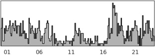
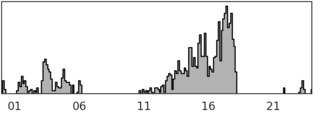
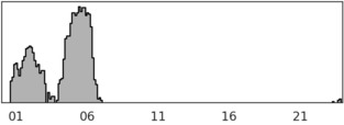
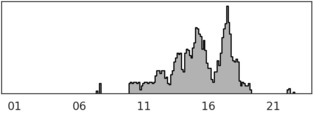
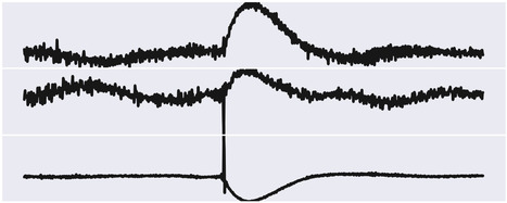
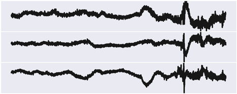
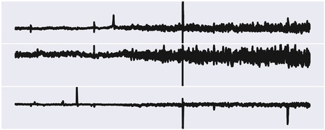
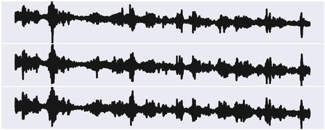
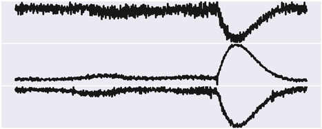
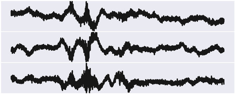
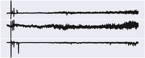
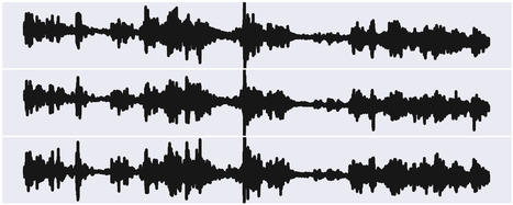
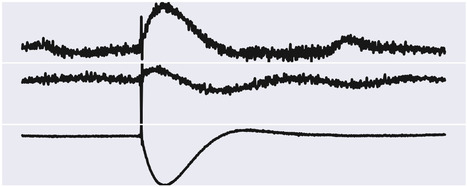
(a) Cluster in $51.2\,$s scale

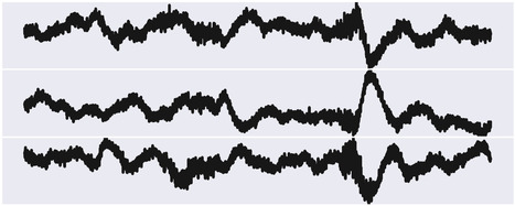
(b) Cluster in $3.4\,$m scale

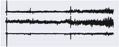
(c) Cluster in $54.6\,$m scale

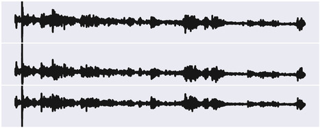
(d) Cluster in $54.6\,$m scale

Figure 2: A selection of clusters over four scales.

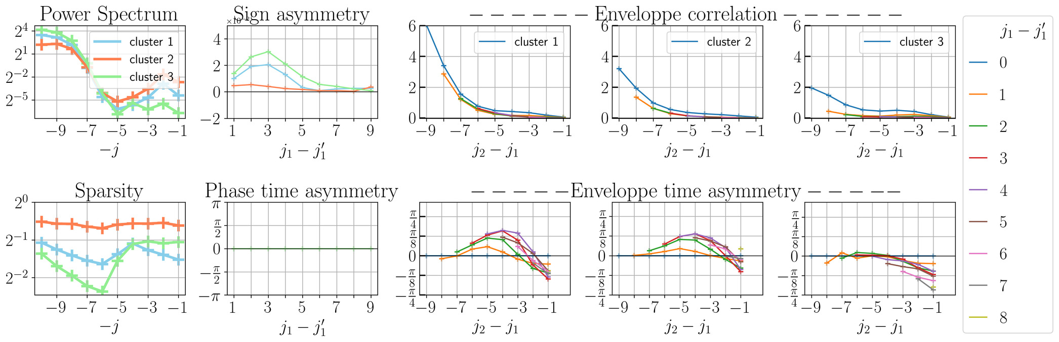
Figure 3: Illustration of the scattering covariance discriminative power for three identified clusters with large time-scales. Cluster 1 has been identified as regional wind. Cluster 2 contains background seismic noises. Cluster 3 consists of signals with many glitches which are transient events. Like cluster 2, cluster 1 shows a long-range dependence structure (“envelope correlation”) with the same time-asymmetry structure. However, it differs significantly from a standard background noise by its sparsity coefficients ($\underset{}{\operatorname{Ave}}\,{|Wx|}$) which are lower, especially at mid-scales, as the result of the presence of ringing oscillations structures in recorded Martian wind.

Martian ambient signals are composed of signals from multiple sources with different time-scales. At short time-scales we expect to see for example transient one-sided pulse called glitches (tens of seconds long) [44], which are likely to come from thermal cracks within the instruments’ subsystem, or atmospheric signals such as dust devils, which are local low pressure structures moving along the ambient wind (tens of seconds long) [45]. On the other hand, at longer time-scale, we expect to see different phenomena such as regional wind whose direction and speed changes over time. Such atmospheric phenomena are strongly dependent on the temperature and thus, they will have strong dependency with the local time at the station [45]. While more in depth investigation will be required to fully uncover the nature of different clusters that were detected by our study, the results we obtained already show that the multi-scale approach is successful in distinguishing such different phenomena that are observed in the Martian data. For example, at the finest time-scale, we identified a cluster that clearly captures glitches (see Figure 2(a)). The top row in Figure 2 shows the time histograms of events in each cluster aggregated over the days July 3–11, 2019, as well as, three component, likely waveforms for each cluster. These waveforms show a clear one-sided pulse that is how a typical glitch waveform looks like. It is interesting that events in such cluster occur throughout the Martian day while it has some tendency to cluster around the sunset (horizontal axis on the time histograms is one Martian day). This is reasonable since glitches are thought to be related to thermal cracks, they tend to concentrate at sunset time when we see large temperature variation from day to night. When focusing on mid to large time-scale results (Figures 2(b)–2(d)), we start to see larger scale phenomena that were not captured in the fine-scale clusters, e.g., Figure 2(d) shows some characteristic waveforms with a sharp onset and a following ringing oscillations. Such waveforms are observed when a strong wind gusts is blowing. This is also consistent with the distribution of the cluster, which is localized in time. Atmospheric activities are day-to-day periodic, and we know that wind will be blowing from a certain direction with known local time [45]. Large-scale clusters can be further analyzed by visualizing their scattering covariance representation (see Figure 3). The clusters for the larger scales tend to be more localized in time as opposed to the finer time-scales that tend to be spread among the whole day. This might imply that the algorithm is detecting signals from regional atmospheric activities that are clustered separately depending on the polarization (i.e., the wind direction).

6.2 Separation of prominent sources

The cluster in Figure 2(c) in addition to glitches (one-sided pulses) contains atmospheric signals related to the sunrise based on the cluster’s time histogram and the sudden increase in waveform amplitude. To separate the glitches, we select a “non-glitch” prior cluster at the finest scale, characterized by a concentrated time histogram during the night and before sunrise, which doesn’t show any glitch visually. This selection allows us to separate the background noise from the glitches (see Figure 4). As mentioned in the previous sections, larger-scale clusters are primarily determined based on background noise characteristics. For instance, the cluster in Figure 2(a) can be recognized as the cluster associated with wind-related atmospheric events. While wind information is valuable for studying the atmospheric conditions on Mars, its presence masks the seismic signal. Leveraging the multi-scale approach of our method, we can effectively isolate the wind’s influence (see Figure 5) and separate it from seismic data.

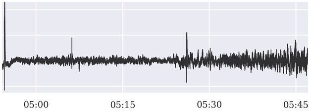
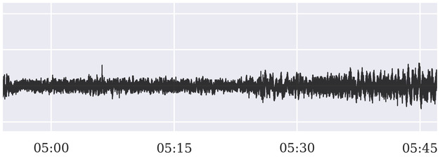
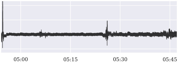
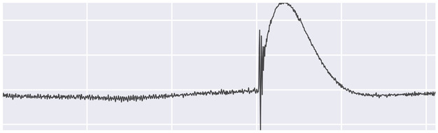
(a) Raw waveform

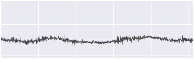
(b) Deglitched

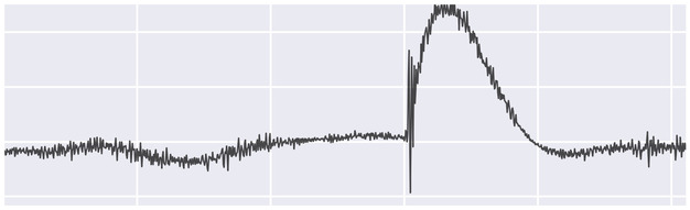
(c) Separated glitch

Figure 4: Deglitching a waveform containing atmospheric-related effects due to sunrise. The second row zooms in on a glitch removed in the first row.

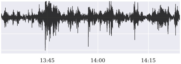
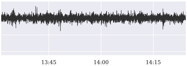
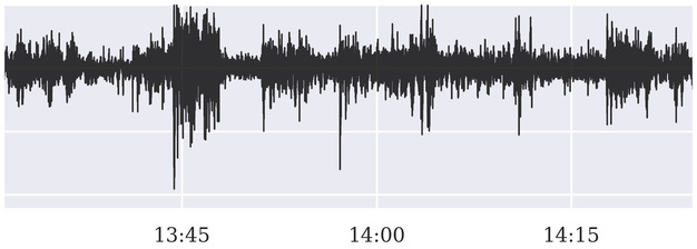
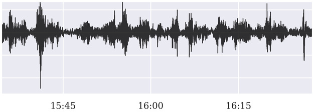
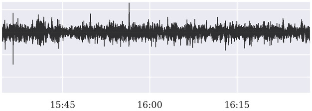
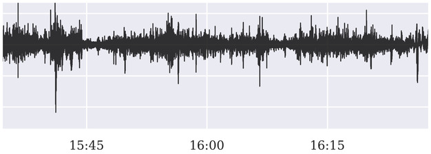
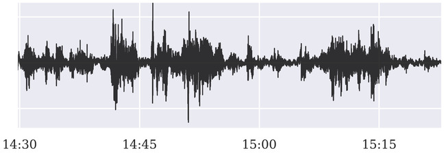
(a) Raw waveform

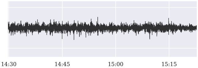
(b) Wind separated

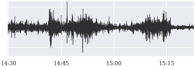
(c) Estimated wind

Figure 5: Removing atmospheric related effects due to wind. The time-scales of the raw waveform and used cluster to extract prior information are $54.6\,$m and $3.4\,$m, respectively.

7 Conclusions

To achieve faithful source separation, prior knowledge on the sources is crucial. Unsupervised source separation methods offer a solution when expert knowledge is limited, as they can learn to extract sources solely from a dataset of source mixtures. However, addressing data with sources of varying time-scales requires an architecture with appropriate inductive biases. In our work, we propose an approach using a factorial Gaussian-mixture variational autoencoder (fVAE) nested within the wavelet scattering covariance representation. Our results on data from NASA’s InSight mission demonstrate the effectiveness of the fVAE in clustering sources at different time-scales, which in turn enables unsupervised source separation by leveraging prior knowledge from the clusters. This approach makes minimal assumptions about the sources and provides a truly unsupervised method for source separation in non-stationary time-series with multi-scale sources. Future work involves amortizing the source separation optimization problem, allowing for end-to-end training.

8 Acknowledgments

Maarten V. de Hoop acknowledges support from the Simons Foundation under the MATH + X program, the National Science Foundation under grant DMS-2108175, and the corporate members of the Geo-Mathematical Imaging Group at Rice University.

Appendix A Organization of the Supplementary Material

Appendix B presents the description of the Scattering Covariance representation $\Psi(\mathbf{x})$. It begins by introducing the main properties of the wavelet filters used in this paper and providing a brief overview of scattering networks [20]. In Appendix C, we delve into the architecture of factorial variational autoencoders (fVAEs). Furthermore, Appendix D provides a detailed description of all the hyperparameters involved in the seismic data example from Mars. In Appendix E, the complete set of clusters across all time scales related to the Mars data example is presenred, along with interpretations regarding multiple clusters. The stability of the clusters, as the random number generator seed value is varied, is summarized in Appendix F. Appendix G concludes our discussion on the results obtained from the Mars dataset by exploring the effect of season changes on the recorded seismic signal. Finally, we present a stylized numerical experiment in Appendix H with carefully curated multi-scale sources to further demonstrate the ability of our method in unsupervised multi-scale clustering and source separation.

Appendix B Background information on wavelet scattering covariance

B.1 Wavelets

A wavelet $\psi(t)$ has a fast decay away from $t=0$, polynomial or exponential for example, and a zero-average $\int\psi(t)\,{\rm d}t=0$. We normalize $\int|\psi(t)|\,dt=1$. The wavelet transform computes the variations of a signal $x$ at each dyadic scale $2^{j}$ with

$$\mathbf{W}\mathbf{x}(t,j)=\mathbf{x}\star\psi_{j}(t)~{}~{}\mbox{where}~{}~{}\psi_{j}(t)=2^{-j}\psi(2^{-j}t).$$

We use a complex wavelet $\psi$ having a Fourier transform $\widehat{\psi}({\omega})=\int\psi(t)\,e^{-i{\omega}t}\,{\rm d}t$ which is real, and whose energy is mostly concentrated at frequencies ${\omega}\in[{\pi},{2}\pi]$. It results that $\widehat{\psi}_{j}(\omega)=\widehat{\psi}(2^{j}\omega)$ is non-negligible mostly in ${\omega}\in[2^{-j}\pi,2^{-j+1}\pi]$.

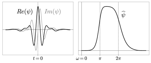
Figure 6: Left: complex Battle-Lemarié wavelet $\psi(t)$ as a function of $t$. Right: Fourier transform $\widehat{\psi}(\omega)$ as a function of ${\omega}$.

We impose that the wavelet $\psi$ satisfies the following energy conservation law called Littlewood-Paley equality

$$\forall\omega>0~{}~{},~{}~{}\sum_{j=-\infty}^{+\infty}|\widehat{\psi}(2^{j}\omega)|^{2}=1.$$ (11)

A Battle-Lemarié wavelet, see Figure 6, is an example of such wavelet. The wavelet transform is computed up to a largest scale $2^{J}$ which is smaller than the signal size $d$. The signal lower frequencies in $[-2^{-J}\pi,2^{-J}\pi]$ are captured by a low-pass filter $\varphi_{J}(t)$ whose Fourier transform is

$$\widehat{\varphi}_{J}(\omega)={\Big{(}\sum_{j=J+1}^{+\infty}|\widehat{\psi}(2^{j}\omega)|^{2}\Big{)}^{1/2}}.$$ (12)

One can verify that it has a unit integral $\int\varphi_{J}(t)\,{\rm d}t=1$. To simplify notations, we write this low-pass filter as a last scale wavelet $\psi_{J+1}=\varphi_{J}$, and $\mathbf{W}\mathbf{x}(t,J+1)=\mathbf{x}\star\psi_{J+1}(t)$. By applying the Parseval formula, we derive from (11) that for all $\mathbf{x}$ with $\|\mathbf{x}\|^{2}=\int|\mathbf{x}(t)|^{2}\,dt<\infty$

$$\|\mathbf{W}\mathbf{x}\|^{2}=\sum_{j=-\infty}^{J+1}\|\mathbf{x}\star\psi_{j}\|^{2}=\|\mathbf{x}\|^{2}.$$

The wavelet transform $\mathbf{W}$ preserves the norm and is therefore invertible, with a stable inverse.

B.2 Wavelet Scattering Networks

A scattering network is a convolutional neural network with wavelet filters. In this paper we choose a simple 2-layer architecture with modulus non-linearity:

$$S\mathbf{x}:=\big{(}\mathbf{W}\mathbf{x},\mathbf{W}|\mathbf{W}\mathbf{x}|\big{)}.$$

The wavelet operator $\mathbf{W}$ is the same at the two layers, it uses $J=8$ predefined Battle-Lemarié complex wavelets that are dilated from the same mother wavelet by powers of $2$, yielding one wavelet per octave.

The first layer extracts $J+1$ scale channels $\mathbf{x}\star\psi_{j}(t)$, corresponding to $J$ band-pass and $1$ low-pass wavelet filters. The second layer is $\mathbf{W}|\mathbf{W}\mathbf{x}|(t;j_{1},j_{2})=|\mathbf{x}\star\psi_{j_{1}}|\star\psi_{j_{2}}(t)$. It is non-negligible only if $j_{1}<j_{2}$. Indeed, the Fourier transform of $|X\star\psi_{j_{1}}|$ is mostly concentrated in $[-2^{-j_{1}}\pi,2^{-j_{1}}\pi]$. If $j_{2}\leq j_{1}$ then it does not intersect the frequency interval $[2^{-j_{2}}\pi,2^{-j_{2}+1}\pi]$ where the energy of $\widehat{\psi}_{j_{2}}$ is mostly concentrated, in which case $S\mathbf{x}(t;j_{1},j_{2})\approx 0$.

Instead of the modulus $|\cdot|$ we could use another non-linearity that preserves the complex phase, however it does not improve significantly the results in this paper.

B.3 Wavelet Scattering Covariance

The wavelet scattering covariance ${\mathbb{E}}\{S(\mathbf{x})S(\mathbf{x})^{\top}\}$ captures scale dependencies which are crucial to characterize non-Gaussian stochastic processes [19]. We detail its coefficients and its main properties in the case of a stationary signal $\mathbf{x}$, more details can be found in [19]. Note however that the paper proposes a extension of this representation to non-stationary signals that relies on a stationary representation averaged on multiple time-scales.

The large matrix ${\mathbb{E}}\{S(\mathbf{x})S(\mathbf{x})^{\top}\}$ is composed of 3 sub-matrices.

$${\mathbb{E}}\begin{bmatrix}\mathbf{W}\mathbf{x}\left(\mathbf{W}\mathbf{x}\right)^{\top}&\mathbf{W}\mathbf{x}\left(\mathbf{W}|\mathbf{W}\mathbf{x}|\right)^{\top}\\ \mathbf{W}|\mathbf{W}\mathbf{x}|\left(\mathbf{W}\mathbf{x}\right)^{\top}&\mathbf{W}|\mathbf{W}\mathbf{x}|\left(\mathbf{W}|\mathbf{W}\mathbf{x}|\right)^{\top}\end{bmatrix}.$$ (13)

• Correlation matrix ${\mathbb{E}}\{\mathbf{W}\mathbf{x}\left(\mathbf{W}\mathbf{x}\right)^{\top}\}$ considers linear correlations. For processes with a regular power spectrum, different times $t\neq t^{\prime}$ and different scales $2^{j}\neq 2^{j^{\prime}}$ barely correlate due to phase fluctuation [46]. This matrix is thus quasi-diagonal and we only retain its diagonal coefficients ${\mathbb{E}}\{|\mathbf{x}\star\psi_{j}(t)|^{2}\}$. They do not depend upon $t$ because $\mathbf{x}$ is stationary and are estimated through an empirical average

  $$\Psi^{2}(\mathbf{x})[j]=\operatorname{Ave}\big{(}|\mathbf{x}\star\psi_{j}(t)|^{2}\big{)}.$$

  This wavelet power spectrum consists of $J+1$ coefficients.

• Correlation matrix ${\mathbb{E}}\{\mathbf{W}\mathbf{x}\left(\mathbf{W}|\mathbf{W}\mathbf{x}|\right)^{\top}\}$ considers signed interactions between wavelet coefficients. They detect sign-asymmetry and time-asymmetry. Again, for a process with regular power-spectrum, we only retain coefficients correlating same times and same scales of the second wavelet operator. Furthermore, different scale channels having different energies given by the wavelet power spectrum $\Psi^{2}(\mathbf{x})[j]$, we perform a per-channel normalization which yield the estimators

  $$\Psi^{3}(\mathbf{x})[j,j^{\prime}]=\frac{\operatorname{Ave}\big{(}\mathbf{x}\star\psi_{j}(t)\,|\mathbf{x}\star\psi_{j^{\prime}}|\star\psi_{j}(t)\big{)}}{\sqrt{\Psi^{2}(x)[j]}\sqrt{\Psi^{2}(x)[j^{\prime}]}}.$$

  Coefficients $j\leq j^{\prime}$ barely correlate because the Fourier supports of $\mathbf{x}\star\psi_{j}(t)$ and $|\mathbf{x}\star\psi_{j^{\prime}}(t)|$ barely overlap. We thus retain coefficients with $j>j^{\prime}$ which yields $J(J+1)/2$ coefficients.

• Correlation matrix ${\mathbb{E}}\{\mathbf{W}|\mathbf{W}\mathbf{x}|\left(\mathbf{W}|\mathbf{W}\mathbf{x}|\right)^{\top}\}$ captures dependencies between signal envelopes $|\mathbf{W}\mathbf{x}|$ at different scales. Again, we only retain the coefficients correlating same times and same scales on the second wavelet layer. This yields $J(J+1)(J+2)/6$ normalized coefficients for $j^{\prime}_{1}\leq j_{1}<j_{2}$

  $$\Psi^{4}(\mathbf{x})[j_{1},j^{\prime}_{1},j_{2}]=\frac{\operatorname{Ave}\big{(}|\mathbf{x}\star\psi_{j_{1}}|\star\psi_{j_{2}}(t)\,|\mathbf{x}\star\psi_{j^{\prime}_{1}}|\star\psi_{j_{2}}^{*}(t)\big{)}}{\sqrt{\Psi^{2}(x)[j_{1}]}\sqrt{\Psi(x)[j^{\prime}_{1}]}}.$$

The wavelet scattering covariance representation also considers sparsity coefficients at each scale ${\mathbb{E}}\{|\mathbf{W}\mathbf{x}|\}^{2}/{\mathbb{E}}\{|\mathbf{W}\mathbf{x}|^{2}\}$ which characterize non-Gaussianity of the marginal distribution of wavelet coefficients $\mathbf{W}\mathbf{x}$. For $j\leq J$ these consist of $J$ coefficients estimated by

$$\Psi^{1}(\mathbf{x})[j]=\frac{\big{(}\operatorname{Ave}{|\mathbf{x}\star\psi_{j}(t)|}\big{)}^{2}}{\operatorname{Ave}\big{(}{|\mathbf{x}\star\psi_{j}(t)|^{2}}\big{)}}$$

The wavelet scattering covariance representation $\Psi(\mathbf{x})$ contains the four types of coefficients $\Psi(\mathbf{x})=\big{(}\Psi^{1}(\mathbf{x}),\Psi^{2}(\mathbf{x}),\Psi^{3}(\mathbf{x}),\Psi^{4}(\mathbf{x})\big{)}$. It can be separated into real and potentially complex coefficients $\Psi(\mathbf{x})=\big{(}\Psi_{\text{real}}(\mathbf{x}),\Psi_{\text{complex}}(\mathbf{x})\big{)}$. The coefficients $\Psi_{\text{real}}(\mathbf{x})=(\Psi^{1}(\mathbf{x})[j],\Psi^{2}(\mathbf{x})[j],\Psi^{4}(x)[j_{1}=j^{\prime}_{1},j_{2}])$ are always real, while the coefficients $\Psi_{\text{complex}}(\mathbf{x})=(\Psi^{3}(\mathbf{x})[j,j^{\prime}],\Psi^{4}(\mathbf{x})[j^{\prime}_{1}<j_{1},j_{2}])$ may be nonreal complex.

The following proposition presents the main properties of our representation regarding non-Gaussianity, it is proved in [19].

Proposition B.1.

Let $\mathbf{x}$ be a stationary process.

1. If $\mathbf{x}$ is Gaussian then

   $${\mathbb{E}}\{\Psi^{1}(\mathbf{x})\}=\frac{\pi}{4}~{}~{}\text{and}~{}~{}{\mathbb{E}}\{\Psi_{\text{complex}}(\mathbf{x})\}=0.$$

2. If $\mathbf{x}$ is sign-invariant i.e. $\mathbf{x}\overset{d}{=}-\mathbf{x}$ in distribution then

   $${\mathbb{E}}\{\Psi^{3}(x)\}=0.$$

3. If $\mathbf{x}$ is time-reversible i.e. $\mathbf{x}(t)\overset{d}{=}\mathbf{x}(-t)$ then

   $$\mathrm{Im}\,{\mathbb{E}}\{\Psi_{\text{complex}}(\mathbf{x})\}=0.$$

This means that, up to estimation error in replacing the expectation ${\mathbb{E}}$ by an empirical average $\operatorname{Ave}$, our representation detects non-Gaussianity through non-zero coefficients. Beyond that, $\Psi(\mathbf{x})$ is able to quantify different non-Gaussian behaviors, which is be crucial for source separation.

For visualization purpose we only plot the coefficients $\Psi^{2}(\mathbf{x})[j,j^{\prime}]$ averaged on constant log-scale lags $j-j^{\prime}$ and coefficients $\Psi^{4}(\mathbf{x})[j_{1},j^{\prime}_{1},j_{2}]$ on constant log-scale lags $j^{\prime}_{1}-j_{1},j_{2}-j_{1}$. This reduces a lot the number of coefficients. One can prove that for scale invariant processes this reduced set of values actually bears all the information in the scattering covariance [19].

Figure 7 visualizes the scattering covariance for two processes, a Gaussian white noise and a non-Gaussian multifractal noise [47] that exhibits intermittency. It shows sparsity coefficients $\Psi^{1}(\mathbf{x})[j]$, wavelet power spectrum $\Psi^{2}(\mathbf{x})[j]$, sign-asymmetry coefficients $|\Psi^{3}(\mathbf{x})[j,j^{\prime}]|$, phase time-asymmetry coefficients $\mathrm{Arg}\,\Psi^{3}(\mathbf{x})[j,j^{\prime}]$, envelope correlation $|\Psi^{4}(\mathbf{x})[j_{1},j^{\prime}_{1},j_{2}]|$ and envelope time-asymmetry $\mathrm{Arg}\Psi^{4}(\mathbf{x})[j_{1},j^{\prime}_{1},j_{2}]$.

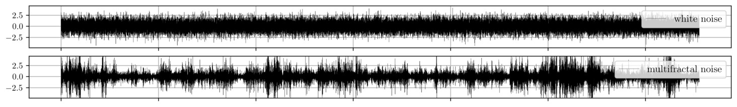
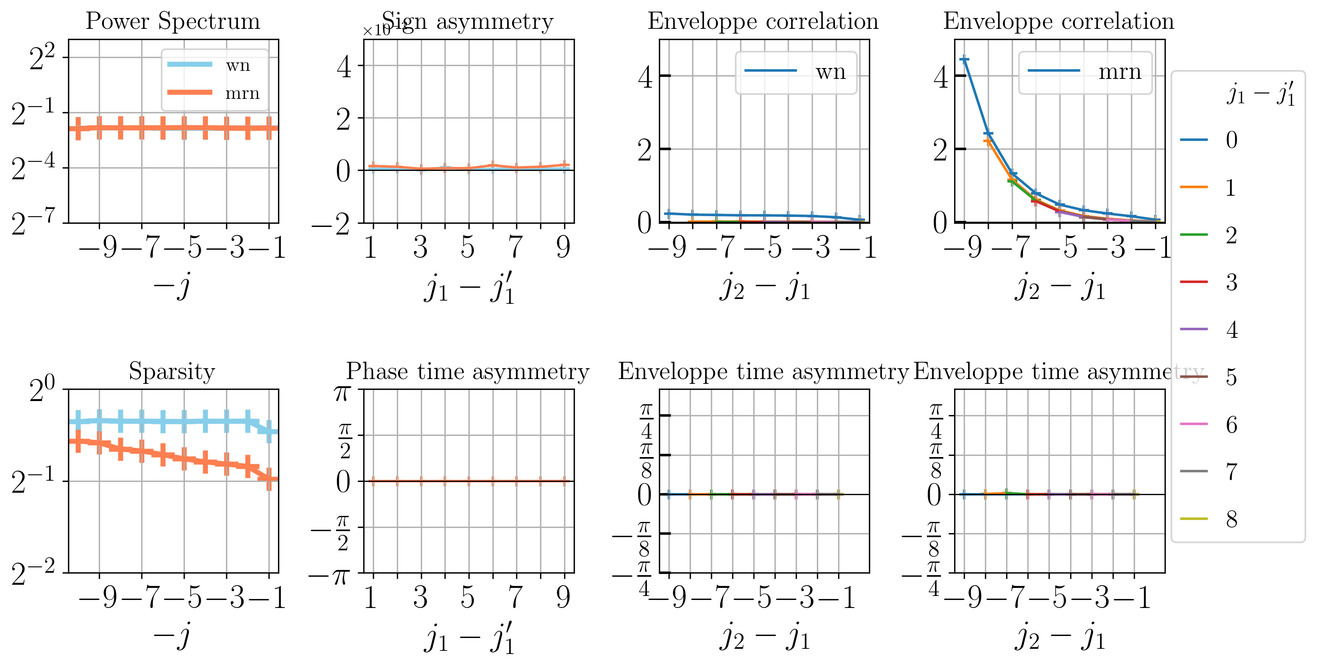
Figure 7: Scattering covariance representation of a Gaussian white noise (wn) and a non-Gaussian multifractal random noise (mrn), both being sign-invariant and time-reversible. Non-flat sparsity coefficients and non-zero envelope correlation coefficients for $j_{1}<j^{\prime}_{1}$ show that the mrn is non-Gaussian with intermittency, as can be seen on its time-series.

Figure 8 and Figure 9 shows two types of clusters obtained by our algorithm at large scale. The first clusters are composed of noisy signals, the second clusters are identified as signals with glitches which are transient events. The figures show that an important variability detected by the scattering covariance is the presence of glitches which results in a sparse signal with sign-asymmetry (Figure 9). Inside the noisy clusters (Figure 8) the level of envelope correlations seems to be another type of variability. More subtly the shape of envelope time-asymmetry varies from a noisy cluster to the other.

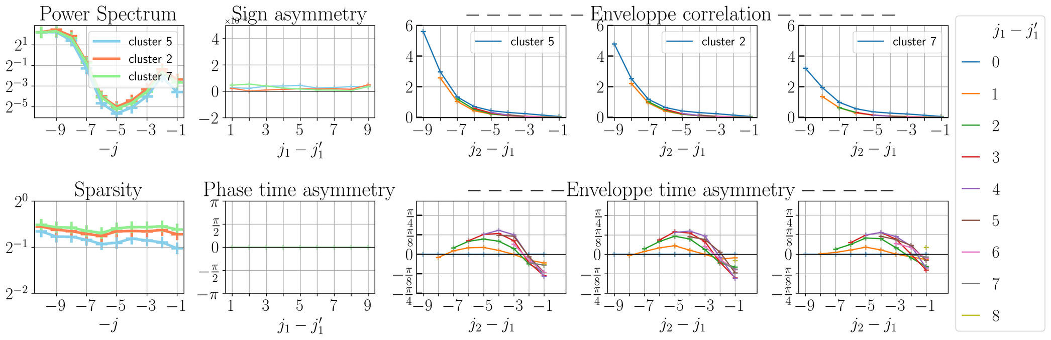
Figure 8: Scattering covariance representation of 3 clusters of Mars seismic data identified as clusters of background noise.

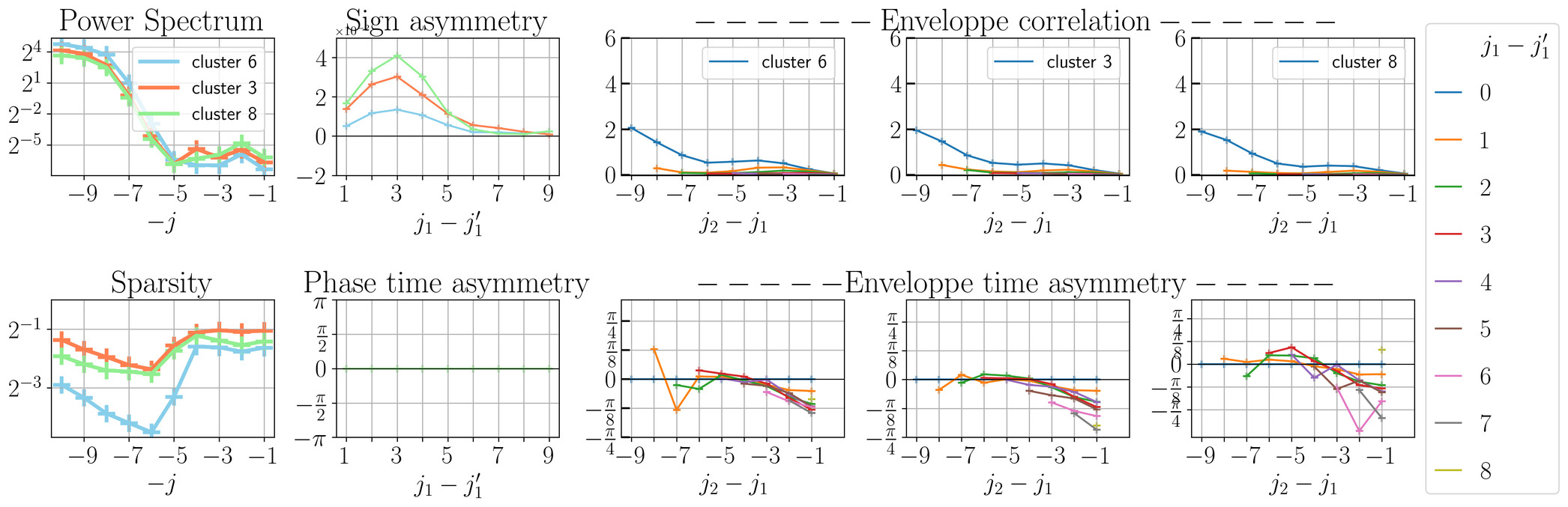
Figure 9: Scattering covariance of Mars clusters obtained from our clustering algorithm. These 3 clusters contain glitches which are transient events. This is detected by sparsity and sign-asymmetry coefficients.

B.4 Scattering cross-covariance

Scattering covariance 13 can be considered between two signals $\mathbf{x}$ and $\mathbf{y}$. We use it to enforce dependency between sources in our source separation algorithm.

The same diagonal reduction presented in the previous section, written $\operatorname{diag}$, applies and it defines the scattering cross-covariance $\Psi(\mathbf{x},\mathbf{y})=\operatorname{Ave}\operatorname{diag}\big{(}S(\mathbf{x})S(\mathbf{y})^{\top}\big{)}$ that captures non-linear non-Gaussian dependencies between signals $\mathbf{x},\mathbf{y}$.

Proposition B.2.

If $\mathbf{x}$ and $\mathbf{y}$ are independent then

$${\mathbb{E}}\{\Psi(\mathbf{x},\mathbf{y})\}=0$$

Proof.

If $\mathbf{x}$ and $\mathbf{y}$ are independent processes then $S(\mathbf{x})$ and $S(\mathbf{y})$ are also independent and thus their covariance is zero. ∎

In our source separation algorithm we seek to impose independence between sources $\mathbf{s}_{1}$ and $\mathbf{s}_{2}$ by enforcing $\Psi(\mathbf{s}_{1},\mathbf{s}_{2})=0$.

Appendix C Factorial variational autoencoder architecture

The architecture of the fVAE primarily relies on fully connected layers. The input consists of concatenated pyramidal wavelet scattering covariances, which are then passed through the joint encoder. This module is composed of a series of fully connected residual blocks, totaling four blocks. Each block includes a fully connected layer that reduces the dimensionality of the concatenated features to a hidden dimension, here set to 1024. This is followed by a Batchnorm layer and LeakyReLU nonlinearity. The output of the residual block is then brought back to the input dimensionality using another fully connected layer, and the result is added to the input (skip connection) to form the output of the residual block. Thanks to the pyramidal scattering covariance representation, the joint encoder with skip connection preserves maximal information from each scale and learns to extract useful information for generative modeling and clustering of representations.

Moving on to the per-scale encoders, the output of the joint encoder is split among different scales, and each scale is fed to a per-scale encoder. These encoders consist of compositions of four fully connected layers, Batchnorm, and LeakyReLU activations. The first layer changes the dimensionality of each scale’s representation to the hidden dimension (1024), while the last layer reduces this hidden dimension to the latent dimension of 32. We parameterize the latent distribution of each scale as a Gaussian mixture model with nine components, where the mean and diagonal covariances are unknown vectors. On the decoding side, the per-scale decoders mirror the per-scale encoders and reconstruct the input multi-scale representation from the latent space.

Appendix D Details regarding experiments with data from Mars

We provide a comprehensive explanation of the various stages involved in our proposed unsupervised multi-scale clustering and source separation method to facilitate the reproducibility of our results.

D.1 Pyramidal wavelet scattering covariance representation

Based on existing studies on seismic data from the InSight mission [44, 45, 43], we selected the finest time-scale to be $51.2\,$seconds. This choice allows us to capture the diversity present in the one-sided pulses. To determine the subsequent time-scales, we multiplied the previous time-scale by a factor of four. While we do not expect to cluster broadband marsquakes [48] due to their infrequent occurrence compared to other sources, we set the largest window size to be $54.6\,$minutes. This window size covers marsquakes and other sources related to atmospheric-surface interactions [45]. Given a sampling rate of 20 samples per second, the aforementioned time-scales correspond to window sizes of $2^{10}$, $2^{12}$, $2^{14}$, and $2^{16}$. By computing the scattering covariances over these time-scales, we obtain $210$-dimensional complex scattering covariance representations for each scale. We split and concatenate the real and imaginary parts of these representations, treating the resulting $420$-dimensional vectors as pyramidal wavelet scattering covariance representations.

D.2 Training details of the factorial variational autoencoder

We utilized the data recorded during 2019 [49] to train the fVAE. During training, we randomly reserved $10\%$ of the data as validation data for tuning a set of hyperparameters. Following the approach of Barkaoui et al. [43], we employed nine clusters at each time-scale. The fVAE was trained using the architecture outlined in section C, employing a hidden dimension of 1024 and a latent dimension of 32. The Adam optimization algorithm [50] was employed with a learning rate of $10^{-3}$. Training was conducted for $1000$ epochs, utilizing a batch size of $16384$. To address non-differentiability concerns, we utilized the Gumbel-Softmax distribution, enabling a differentiable approximate sampling mechanism for categorical variables [23]. The initial temperature parameter for the Gumbel-Softmax distribution was set to $1.0$, and we exponentially decayed the temperature to a minimum value of $0.5$. Training takes approximately eight hours on a Tesla V100.

D.3 Source separation parameters

Throughout the source separation examples, we solve the optimization problem using $1000$ iterations of the L-BFGS optimization algorithm [51]. Below, we provide details for the two source separation examples.

Deglitching. In the glitch separation example, we extract the data to be deglitched from the first cluster at the largest time-scale (see Figure 10d.1 for the time histogram and the first row of Figure 14 for representative waveforms). To formulate the source separation optimization problem, we utilize $50$ data snippets as prior information from the fifth cluster at the finest time-scale (refer to Figure 10a.5 for the time histogram and the fifth row of Figure 11 for representative waveforms). The time histogram of this cluster overlaps with portions of the time histogram in Figure 10d.1, but its waveforms do not contain glitches (visually), allowing us to separate everything except for glitches.

Removing wind-related atmospheric effects. In this example, we select three windows of data containing wind-related effects from the second cluster at the largest time-scale (see Figure 10d.2 for the time histogram and the second row of Figure 14 for representative waveforms). For prior information, we choose $300$ data snippets from the eighth cluster at the second finest time-scale (see Figure 10b.8 for the time histogram and the eighth row of Figure 12 for representative waveforms). Similar to the previous example, we select the prior cluster primarily based on the significant overlap of its time histogram with the time histogram in Figure 10d.2, while visually lacking the wind-related features, namely, a sharp onset and subsequent ringing oscillations.

Appendix E Identified clusters and their representative waveforms

In this section, we present the complete set of nine clusters identified by the fVAE across four different time scales: $51.2\,$seconds, $3.4\,$minutes, $13.6\,$minutes, and $54.6\,$ minutes. Figure 10 displays the time histograms for these clusters, aggregating data from July 3–11, 2019. The horizontal axis of the histograms represents one Martian day. Each column in Figure 10 corresponds to a time scale, with the time scales increasing from the left-most column to the right.

Additionally, we provide the representative waveforms for each cluster at all time scales. These waveforms are the ones that have been clustered with a high probability, indicating their proximity to the corresponding Gaussian mixture mode. Figures 11–14 depict these waveforms for time scales of $51.2\,$seconds, $3.4\,$minutes, $13.6\,$minutes, and $54.6\,$minutes, respectively. Each figure showcases four waveforms per cluster, with each cluster represented in a row. The ordering of clusters between the rows of Figure 10 and Figures 11–14 is consistent. For example, the cluster associated with the time histograms in the first row of the figure corresponds to the clusters in the first rows of Figures 11–14.

When we compare results from different time scales, we see more clusters with narrow time window. For example, Figure 10a.2 shows a very broad distribution of the cluster with a weak peak around 16:00-21:00 local time. Such ubiquitous distribution is also seen in Figure 10b.5 but is less clear for longer time scales. Indeed, the distribution is generally well localized in time in the right-most column of Figure 10 with the longest time scale. This implies that the clusters with smaller time-scale are less dependent on temperature or atmospheric conditions. On the other hand, most of the cluster in the long time scale are likely to be controlled more by temperature with diurnal variation well correlated with the local time. The former case is more compatible with transient artifacts such as glitches, while the latter case implies for example regional winds that are known to blow at specific atmospheric conditions.

To further investigate the origin of the clusters, we will now discuss the waveform of each cluster. One typical example is glitch cluster that we see in the second row of Figure 11 and the fifth row of Figure 12. These are the clusters that are distributed broadly among the local time (cf. Figure 10) with some enhancement either at the sunset time or in morning or during the night. This will be informative to understand the source of glitches. Interestingly, we see other clusters such as the third row in Figure 11, which has similar waveform as glitched but has non-typical glitch waveform. This cluster is distributed differently and the difference might be coming from the difference in their origin and requires further investigations.

a.1

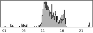
b.1

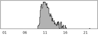
c.1

d.1

a.2

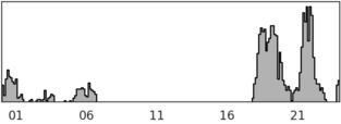
b.2

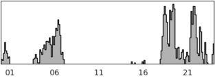
c.2

d.2

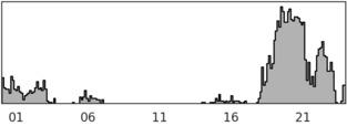
a.3

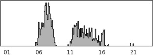
b.3

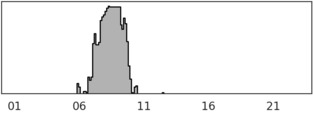
c.3

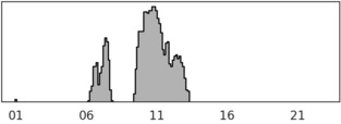
d.3

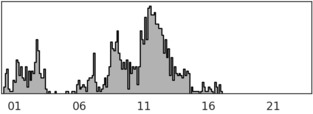
a.4

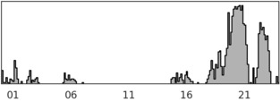
b.4

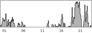
c.4

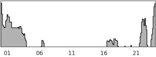
d.4

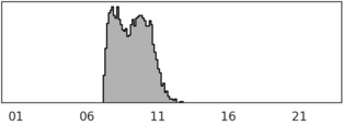
a.5

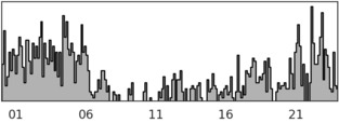
b.5

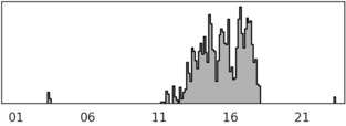
c.5

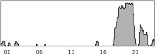
d.5

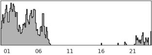
a.6

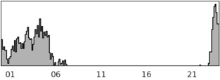
b.6

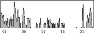
c.6

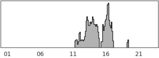
d.6

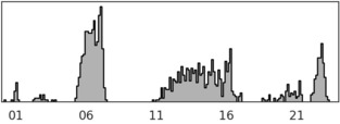
a.7

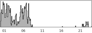
b.7

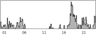
c.7

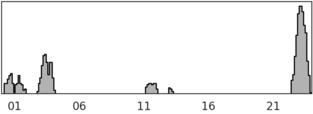
d.7

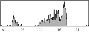
a.8

b.8

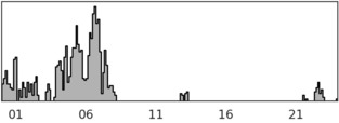
c.8

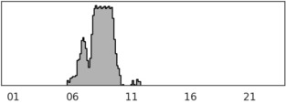
d.8

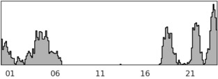
a.9

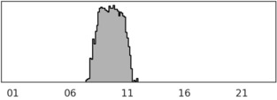
b.9

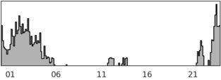
c.9

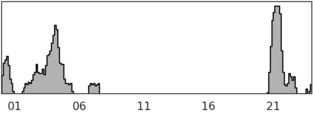
d.9

Figure 10: A complete set of nine identified clusters within four different scales. From left to right, each column is associated with nine clusters representing each time-scale, namely, $51.2\,$seconds (Figures 10a.1–10a.9) , $3.4\,$minutes (Figures 10b.1–10b.9), $13.6\,$minutes (Figures 10c.1–10c.9), and $54.6\,$minutes (Figures 10d.1–10d.9) scales, respectively. The order of clusters within each scale is not significant, and therefore, the same cluster index across scales does not hold any meaning.

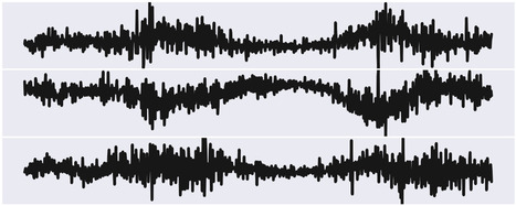
a.1

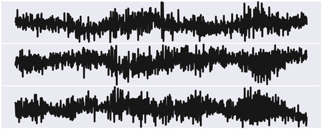
b.1

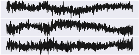
c.1

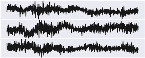
d.1

a.2

b.2

c.2

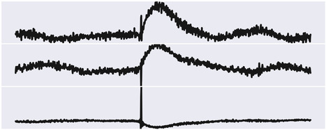
d.2

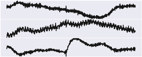
a.3

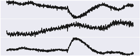
b.3

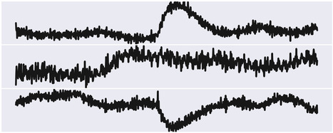
c.3

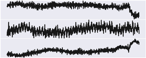
d.3

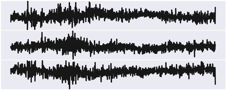
a.4

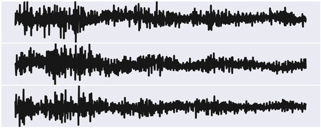
b.4

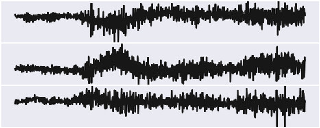
c.4

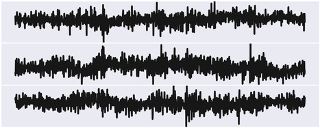
d.4

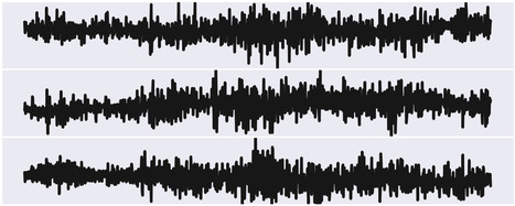
a.5

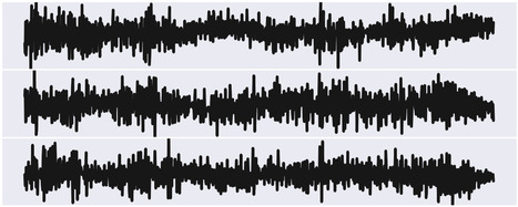
b.5

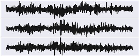
c.5

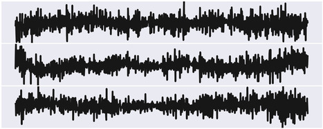
d.5

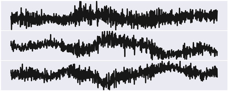
a.6

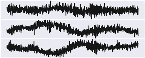
b.6

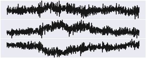
c.6

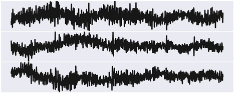
d.6

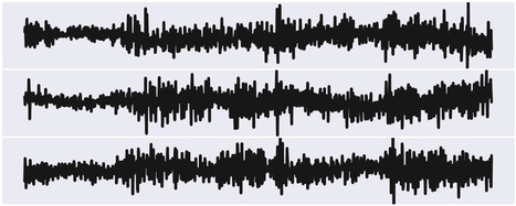
a.7

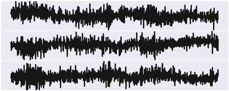
b.7

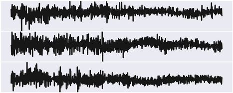
c.7

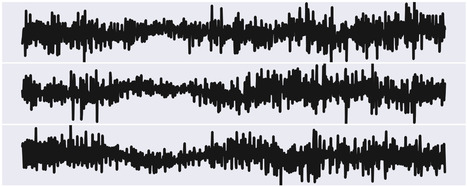
d.7

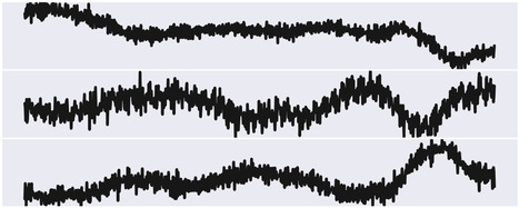
a.8

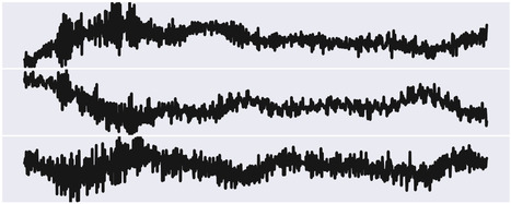
b.8

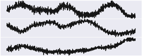
c.8

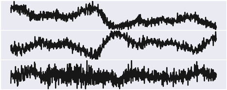
d.8

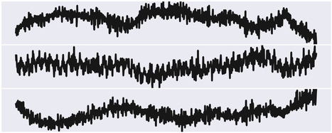
a.9

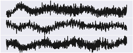
b.9

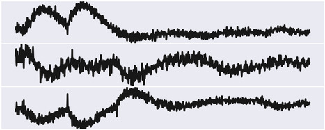
c.9

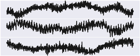
d.9

Figure 11: Waveforms in time-scale of $51.2\,$seconds, with each row from top to bottom illustrating four waveforms corresponding to clusters one to nine in this time-scale (cf. Figures 10a.1–10a.9), respectively.

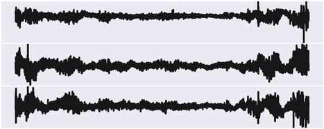
a.1

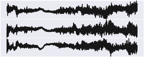
b.1

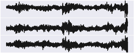
c.1

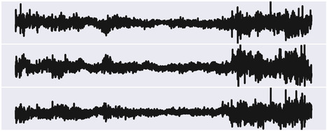
d.1

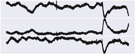
a.2

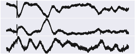
b.2

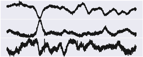
c.2

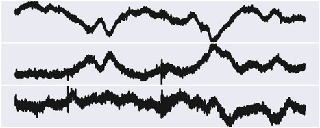
d.2

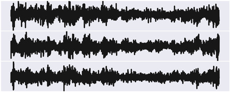
a.3

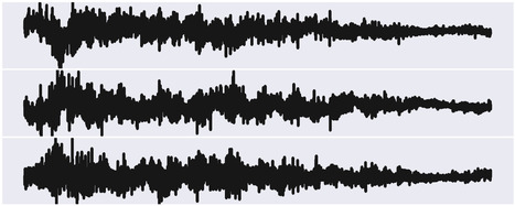
b.3

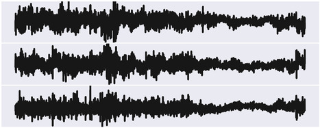
c.3

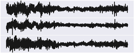
d.3

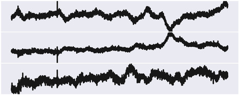
a.4

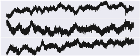
b.4

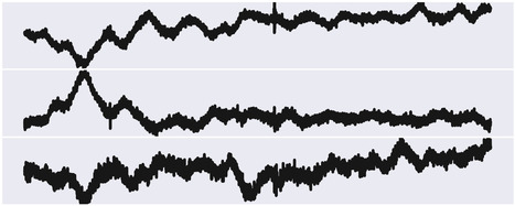
c.4

d.4

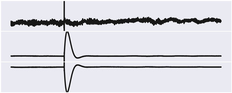
a.5

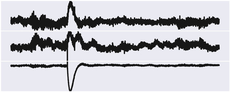
b.5

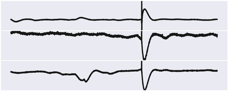
c.5

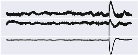
d.5

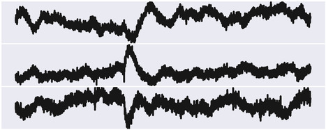
a.6

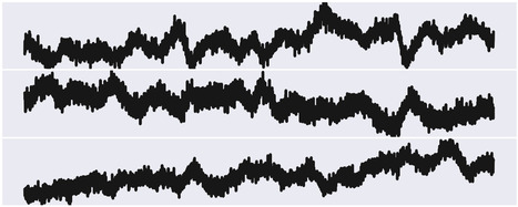
b.6

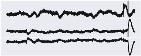
c.6

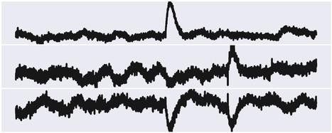
d.6

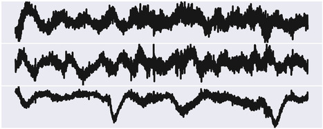
a.7

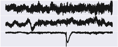
b.7

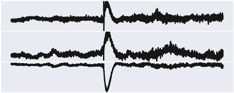
c.7

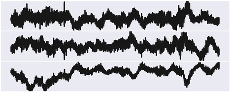
d.7

a.8

b.8

c.8

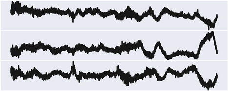
d.8

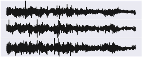
a.9

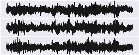
b.9

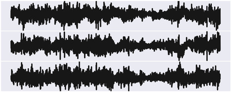
c.9

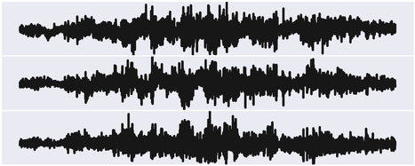
d.9

Figure 12: Waveforms in time-scale of $3.4\,$minutes, with each row from top to bottom illustrating four waveforms corresponding to clusters one to nine in this time-scale (cf. Figures 10b.1–10b.9), respectively.

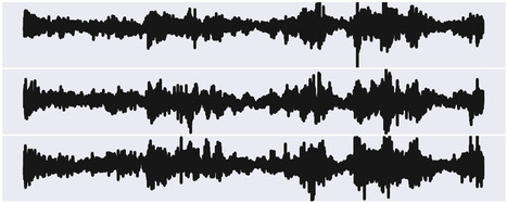
a.1

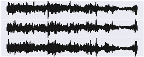
b.1

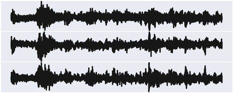
c.1

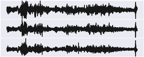
d.1

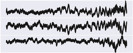
a.2

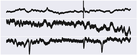
b.2

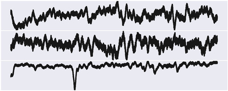
c.2

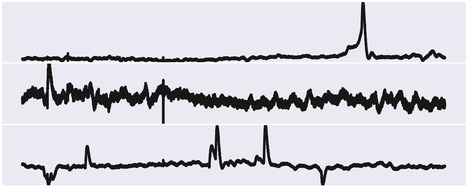
d.2

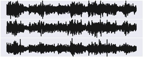
a.3

b.3

c.3

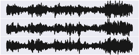
d.3

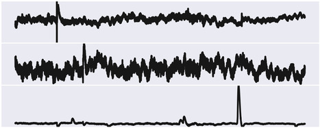
a.4

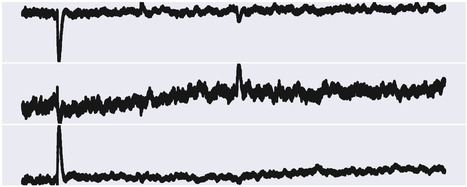
b.4

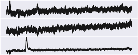
c.4

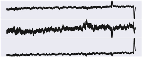
d.4

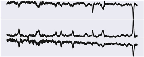
a.5

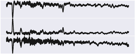
b.5

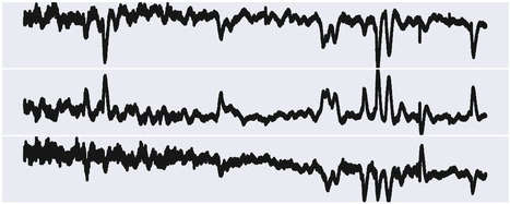
c.5

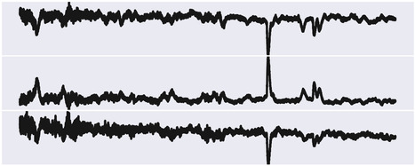
d.5

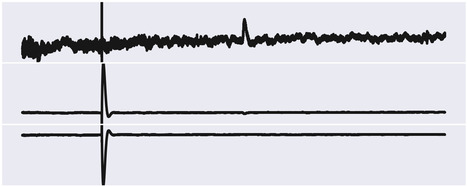
a.6

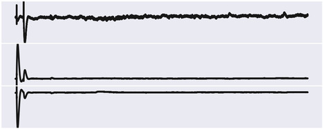
b.6

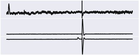
c.6

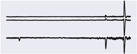
d.6

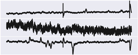
a.7

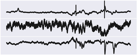
b.7

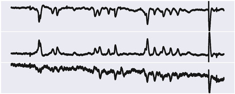
c.7

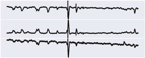
d.7

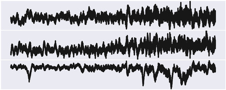
a.8

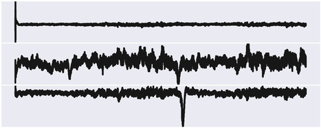
b.8

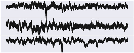
c.8

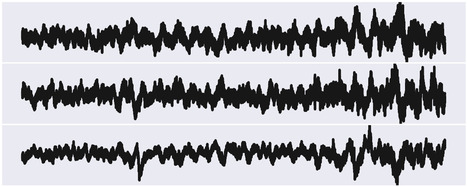
d.8

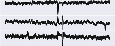
a.9

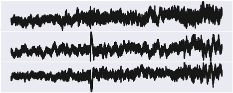
b.9

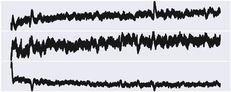
c.9

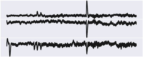
d.9

Figure 13: Waveforms in time-scale of $13.6\,$minutes, with each row from top to bottom illustrating four waveforms corresponding to clusters one to nine in this time-scale (cf. Figures 10c.1–10c.9), respectively.

a.1

b.1

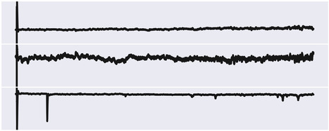
c.1

d.1

a.2

b.2

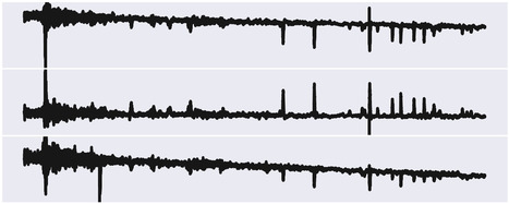
c.2

d.2

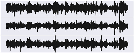
a.3

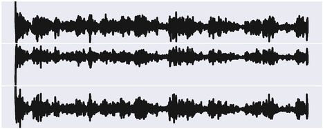
b.3

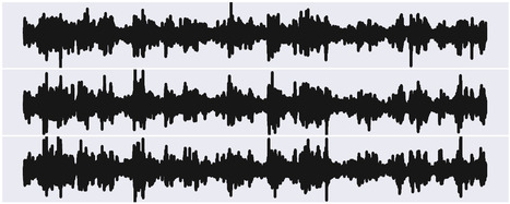
c.3

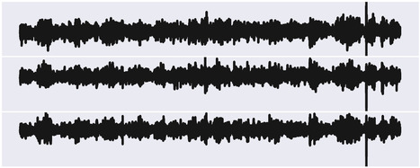
d.3

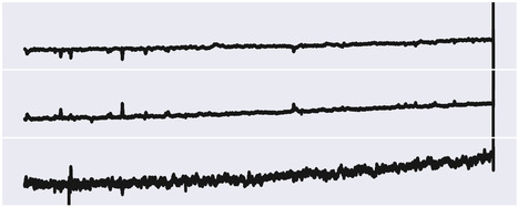
a.4

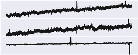
b.4

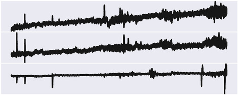
c.4

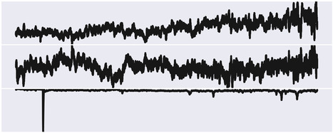
d.4

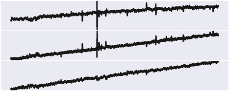
a.5

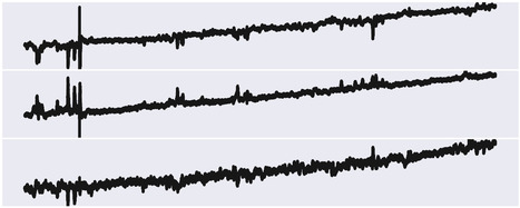
b.5

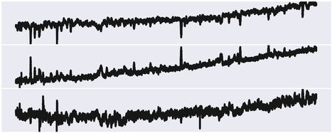
c.5

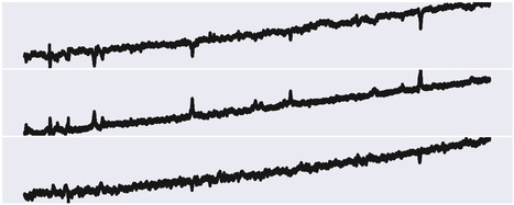
d.5

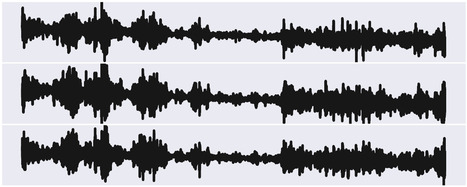
a.6

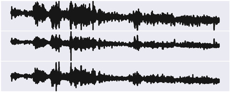
b.6

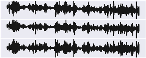
c.6

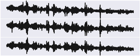
d.6

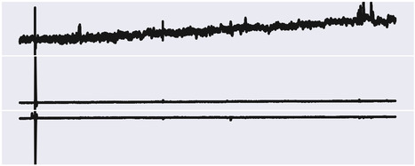
a.7

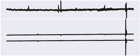
b.7

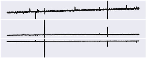
c.7

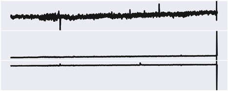
d.7

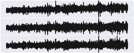
a.8

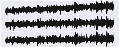
b.8

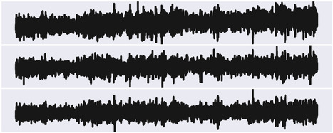
c.8

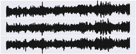
d.8

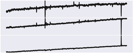
a.9

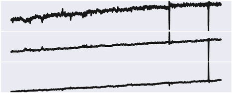
b.9

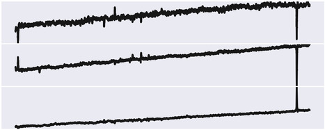
c.9

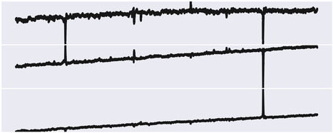
d.9

Figure 14: Waveforms in time-scale of $54.6\,$minutes, with each row from top to bottom illustrating four waveforms corresponding to clusters one to nine in this time-scale (cf. Figures 10d.1–10d.9), respectively.

Appendix F Stability of clusters

To ensure the stability of clusters with respect to the random number generator seed value, we repeat the training process using the same set of hyperparameters with multiple different seeds. To provide insights into the variability of results, we overlay the time-histograms obtained from all seeds for all clusters across all time scales. As the order of clusters is not significant, we group clusters from different seed experiments that are closest to each other. The results are depicted in Figure 15. We observe reasonable robustness in the clusters at finer time scales (left two columns). However, for larger time scales, some clusters exhibit more variation, suggesting that these clusters may have more degrees of freedom. In other words, certain clusters at larger time scales may not be as constrained. This discrepancy might arise from a smaller number of effective windows of data at larger time scales, leading to less robust clusters. Overall, we argue that the clusters are reasonably robust, and any variations can potentially be attributed to the presence of ambiguous data points that lie near the decision boundary.

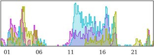
a.1

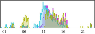
b.1

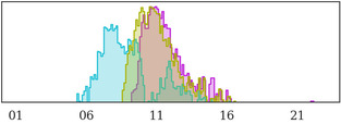
c.1

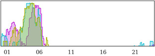
d.1

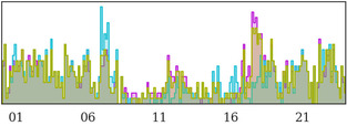
a.2

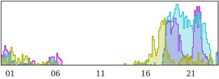
b.2

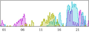
c.2

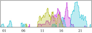
d.2

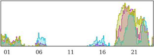
a.3

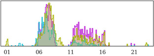
b.3

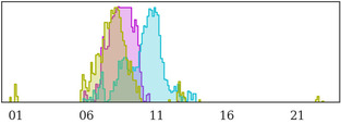
c.3

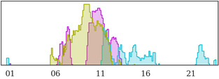
d.3

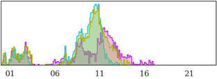
a.4

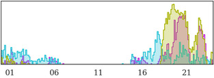
b.4

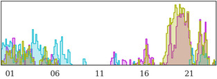
c.4

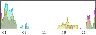
d.4

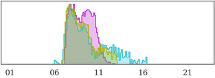
a.5

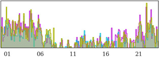
b.5

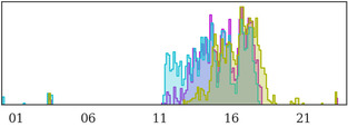
c.5

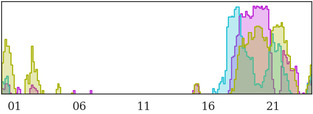
d.5

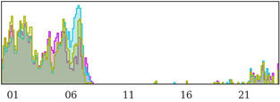
a.6

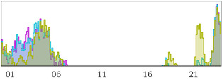
b.6

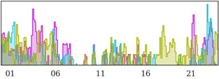
c.6

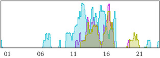
d.6

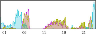
a.7

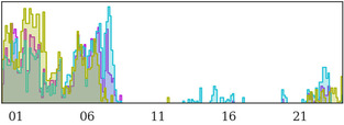
b.7

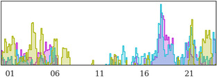
c.7

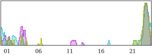
d.7

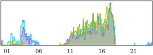
a.8

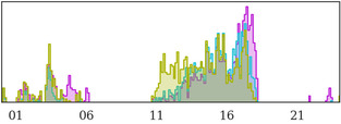
b.8

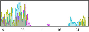
c.8

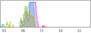
d.8

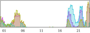
a.9

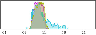
b.9

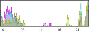
c.9

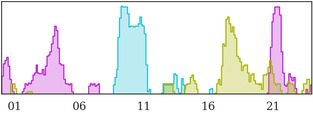
d.9

Figure 15: Cluster robustness to random number generator seed value. A complete set of nine identified clusters within four different scales. From left to right, each column is associated with nine clusters representing each time-scale, namely, $51.2\,$seconds (Figures 15a.1–15a.9) , $3.4\,$minutes (Figures 15b.1–15b.9), $13.6\,$minutes (Figures 15c.1–15c.9), and $54.6\,$minutes (Figures 15d.1–15d.9) scales, respectively. The order of clusters within each scale is not significant, and therefore, the same cluster index across scales does not hold any meaning.

Appendix G Exploring seasonal changes through the lens of fVAE clustering

In order to gain further insights into the atmospheric-surface effects, we conducted an investigation on the impact of seasonal changes on the time histogram of the clusters. We utilized the same training network to cluster data associated with Martian local summer (Sols 306–483) and winter (Sols 625–782). Upon visual inspection, we confirmed that the characteristic waveforms for all clusters at different time scales maintained the same structure as depicted in Figures 11–14. To explore seasonal changes through the lens of clustering, we superimposed the time histograms for all clusters across the four time scales in Figure 16. While we acknowledge that not all variations observed in the time histograms can be solely attributed to seasonal changes (e.g., operational changes of the lander), we identified that certain clusters associated with Martian daytime exhibited a tendency to shift in their peak, e.g., Figures 16a.5, 16b.9, 16c.3, 16c.5, 16d.3, and 16d.6. Furthermore, we also observe that some time histograms decrease in number, e.g., 16b.2, 16b.5, 16c.7, 16d.7, and 16d.8. These two category of changes in histogram are likely to be due to seasonal change in temperature of atmospheric conditions and less a function of seismic activity.

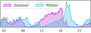
a.1

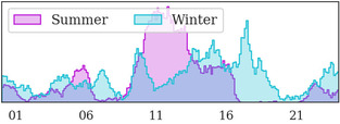
b.1

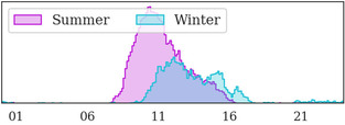
c.1

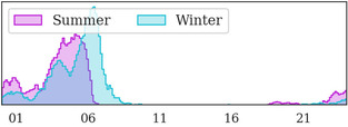
d.1

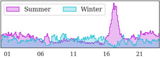
a.2

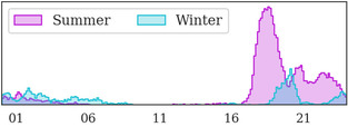
b.2

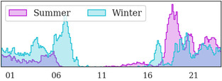
c.2

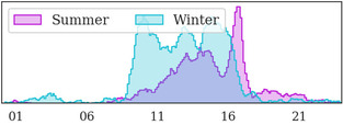
d.2

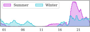
a.3

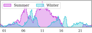
b.3

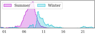
c.3

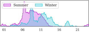
d.3

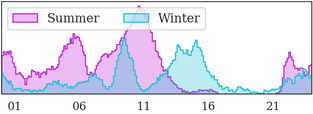
a.4

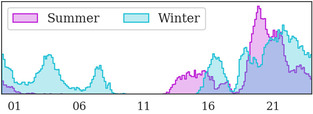
b.4

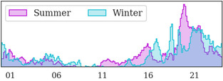
c.4

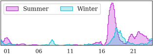
d.4

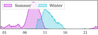
a.5

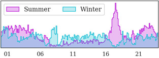
b.5

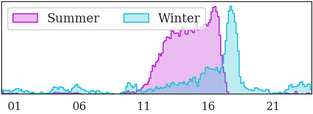
c.5

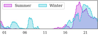
d.5

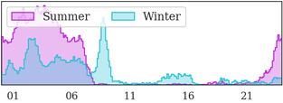
a.6

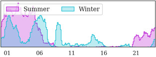
b.6

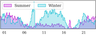
c.6

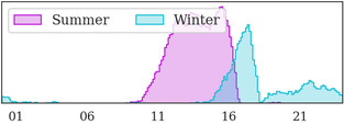
d.6

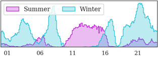
a.7

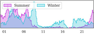
b.7

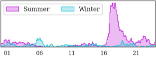
c.7

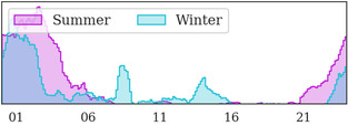
d.7

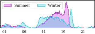
a.8

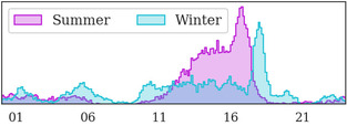
b.8

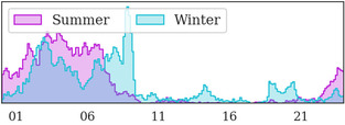
c.8

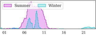
d.8

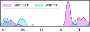
a.9

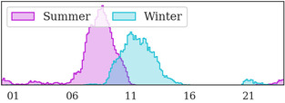
b.9

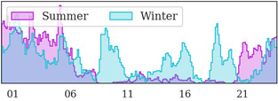
c.9

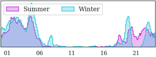
d.9

Figure 16: The effect of seasonal change on clusters. A overlay of time histograms of all nine identified clusters within four different scales where histograms are obtained using data from the Martian local summer (pink) and winter (cyan) data. From left to right, each column is associated with nine clusters representing each time-scale, namely, $51.2\,$seconds (Figures 16a.1–16a.9) , $3.4\,$minutes (Figures 16b.1–16b.9), $13.6\,$minutes (Figures 16c.1–16c.9), and $54.6\,$minutes (Figures 16d.1–16d.9) scales, respectively.

Appendix H Stylized example

We present a multi-scale synthetic dataset (see Figure 17) used to validate our model in the presence of ground truth sources. We first describe how the dataset is constructed and then we present the results of our clustering and source separation algorithm when applied to this dataset.

H.1 Synthetic multi-scale dataset

This dataset is composed of events with three distinct durations $w$ that are outlined below:

• (Large scale, $w=2^{12}$) alternates between two different noises to mimic the change in background noise due to day-night periodicity. The first noise is a white noise $\mathbf{x}_{1}(t)$ and the second one is a multifractal random noise $\mathbf{x}_{2}(t)$ which is a non-Gaussian noise with intermittency [47]. The large scale signal is then $\mathbf{x}_{\text{large}}(t)=(1-\theta(t))\,\mathbf{x}_{1}(t)+\theta(t)\,\mathbf{x}_{2}(t)$ where $\theta(t)$ is equal to $0$ on $[0,w]$ and $1$ on $[w+\eta,2w-\eta]$ for small $\eta$, is $2w$-periodic and has a smooth junction at $t=w$ and at $t=2w$.

• (Medium scale, $w=2^{10}$) exhibits a single type of events which is a turbulent jet recorded in experimental conditions [52]. Each event has a duration $w=2^{10}$ and is placed randomly without overlapping, with as many events as the number of “days” defined at large scale.

• (Fine scales, $w=2^{8}$) is a mixture of two types of transient events with exponential decay. First one $\mathbf{x}_{3}(t)=e^{-|t|}$ is symmetrical in $t=0$, second one $\mathbf{x}_{4}(t)=e^{-t}\mathbf{1}_{t\geq 0}$ is asymmetrical. Each of these signals is randomly positioned in the time-series with four times more occurrence than the number of “days” in our dataset.

The resulting dataset is a long time-series $\mathbf{x}=\mathbf{x}_{\text{large}}+\mathbf{x}_{\text{medium}}+\mathbf{x}_{\text{fine}}$.

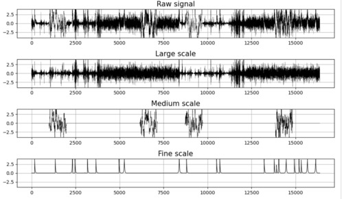
Figure 17: Synthetic multiscale dataset.

H.2 Synthetic data clustering

While we are aware of the underlying sources that create this data, we choose to make an uninformed decision in regards to the number of clusters per scale to mimic a more realistic setting. To this end, we use the same architecture and same hyperparameters as the fVAE trained in the context of clustering and source separation data form Mars, with the distinction that we chose our time-scales for scattering covariance generation based on the duration of sources in our multi-scale dataset.

Figure 18 summarizes the identified clusters after training the fVAE. We can indeed identify different patterns at each time-scale, some of which clearly indicate the multi-scale sources that were used to generate the data. A portion of the clusters are also comprised of at least two of this sources in combination.

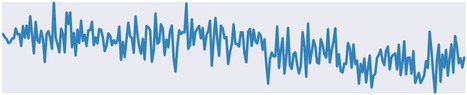
a.1

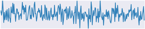
b.1

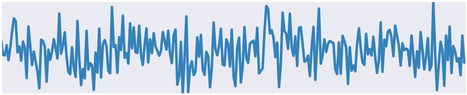
c.1

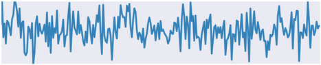
d.1

a.2

b.2

c.2

d.2

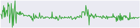
a.3

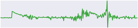
b.3

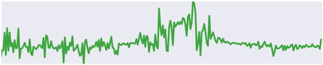
c.3

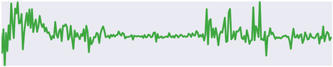
d.3

a.4

b.4

c.4

d.4

a.5

b.5

c.5

d.5

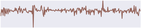
a.6

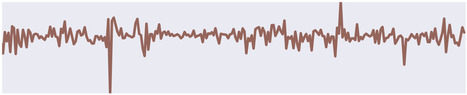
b.6

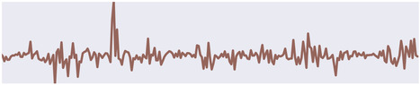
c.6

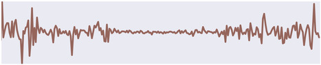
d.6

a.7

b.7

c.7

d.7

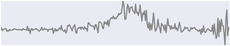
a.8

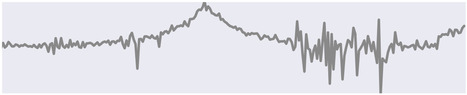
b.8

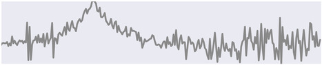
c.8

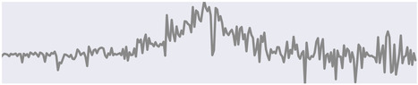
d.8

a.9

b.9

c.9

d.9

Figure 18: Waveforms in time-scale of $256$ sample, with each row from top to bottom illustrating four waveforms corresponding to clusters one to nine in this time-scale, respectively.

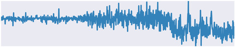
a.1

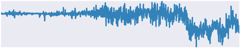
b.1

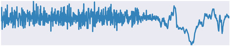
c.1

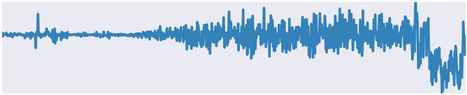
d.1

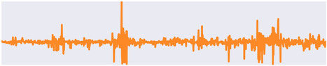
a.2

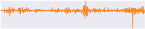
b.2

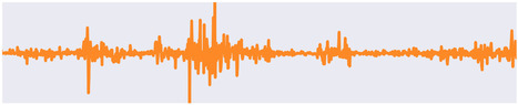
c.2

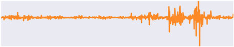
d.2

a.3

b.3

c.3

d.3

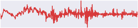
a.4

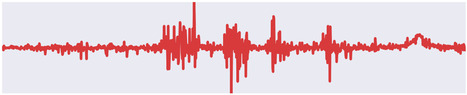
b.4

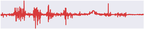
c.4

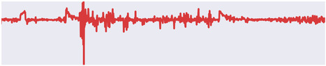
d.4

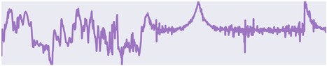
a.5

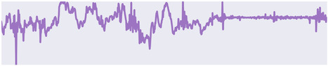
b.5

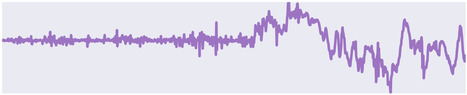
c.5

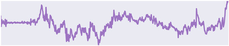
d.5

a.6

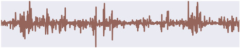
b.6

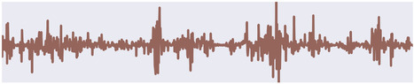
c.6

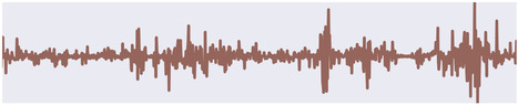
d.6

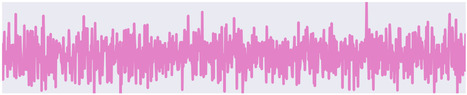
a.7

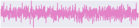
b.7

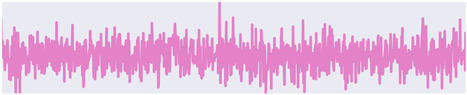
c.7

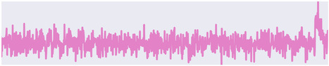
d.7

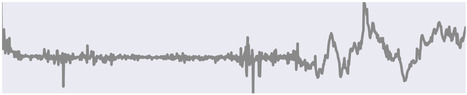
a.8

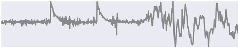
b.8

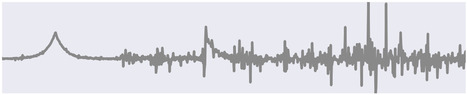
c.8

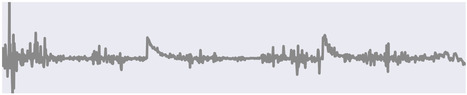
d.8

a.9

b.9

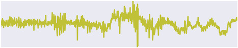
c.9

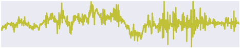
d.9

Figure 19: Waveforms in time-scale of $1024$ sample, with each row from top to bottom illustrating four waveforms corresponding to clusters one to nine in this time-scale, respectively.

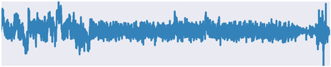
a.1

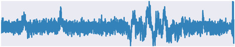
b.1

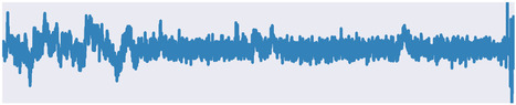
c.1

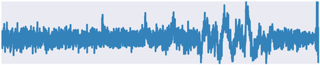
d.1

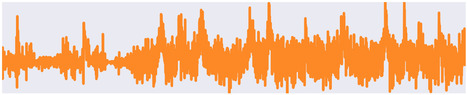
a.2

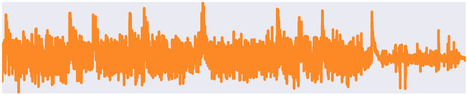
b.2

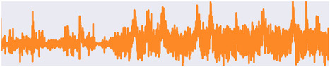
c.2

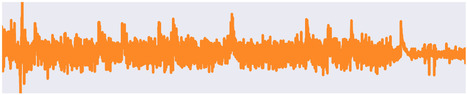
d.2

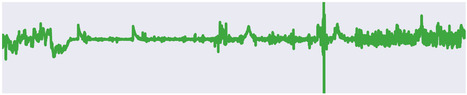
a.3

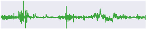
b.3

c.3

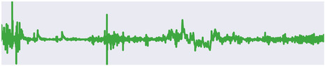
d.3

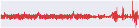
a.4

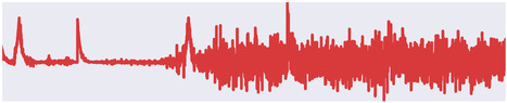
b.4

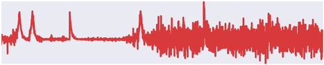
c.4

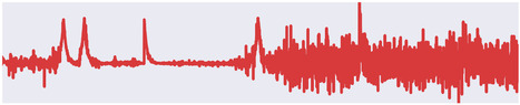
d.4

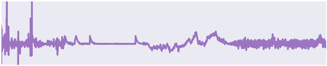
a.5

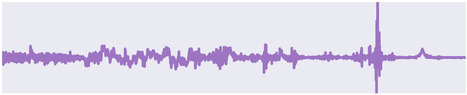
b.5

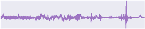
c.5

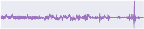
d.5

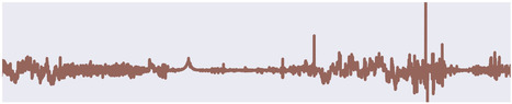
a.6

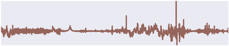
b.6

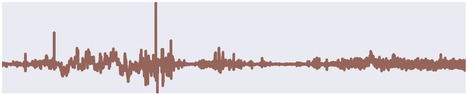
c.6

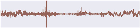
d.6

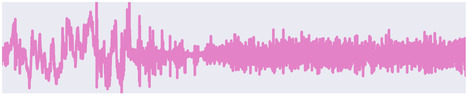
a.7

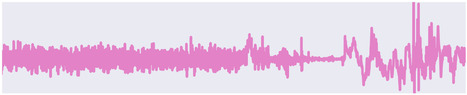
b.7

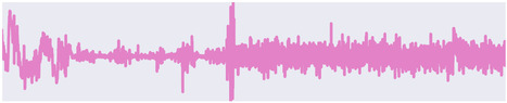
c.7

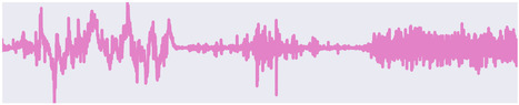
d.7

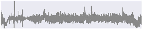
a.8

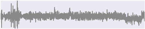
b.8

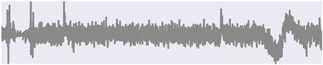
c.8

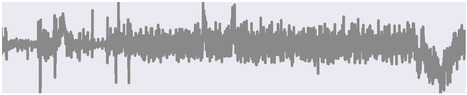
d.8

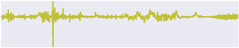
a.9

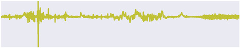
b.9

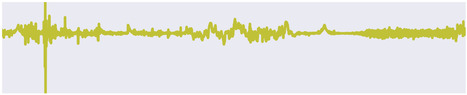
c.9

d.9

Figure 20: Waveforms in time-scale of $4096$ sample, with each row from top to bottom illustrating four waveforms corresponding to clusters one to nine in this time-scale, respectively.

H.3 Synthetic data source separation

Similar to the case with data from Mars, we can identify certain patterns in the obtained clusters and use another cluster as prior information in order to perform per-cluster source separation. Here we exemplify this by separating the medium-scale source that we added from cluster seven in in the largest scale (pink waveforms in Figure 20). To achieve this, we select the pink cluster in Figure 19 as prior cluster as it contains similar background noise to the target cluster but without the medium0scale source. The results of this source separation is shown in Figure 21 for three waveforms. According the the results, our approach has been able to successfully identify and separated the medium-scale source from a set of target waveforms with minimal distortion to the other sources.

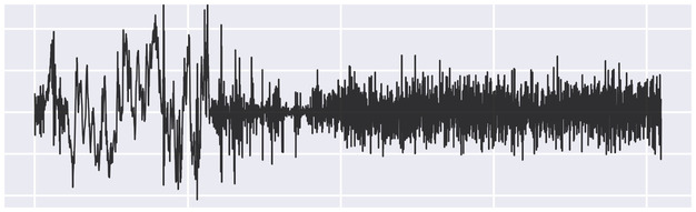
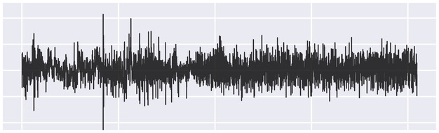
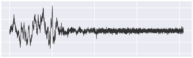
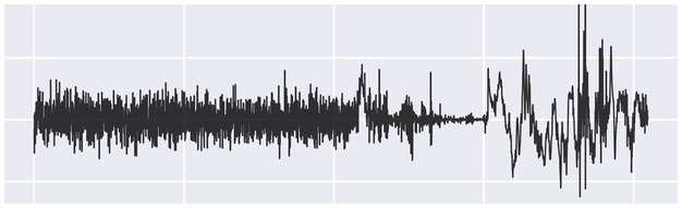
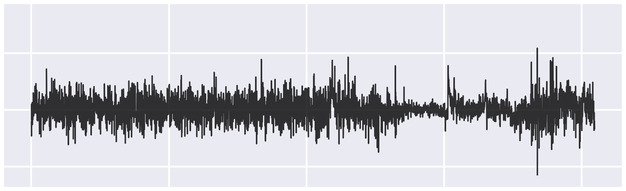
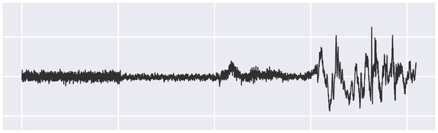
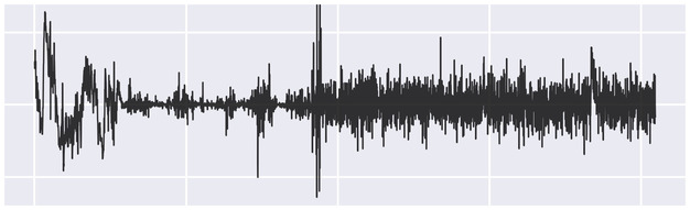
a Mixed waveform

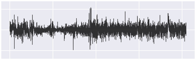
b After source separation

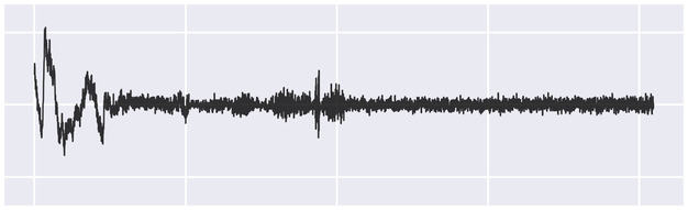
c Medium-scale event separated

Figure 21: Removing the medium-scale source.

References

- Cardoso [1989] J.-F. Cardoso. Source separation using higher order moments. In International Conference on Acoustics, Speech, and Signal Processing, volume 4, pages 2109–2112, 1989. doi: 10.1109/ICASSP.1989.266878.
- Jutten and Herault [1991] Christian Jutten and Jeanny Herault. Blind separation of sources, part I: An adaptive algorithm based on neuromimetic architecture. Signal Processing, 24(1):1–10, 1991. doi: 10.1016/0165-1684(91)90079-X.
- Bingham and Hyvärinen [2000] Ella Bingham and Aapo Hyvärinen. A fast fixed-point algorithm for independent component analysis of complex valued signals. International Journal of Neural Systems, 10(01):1–8, 2000. doi: 10.1142/S0129065700000028.
- Nandi and Zarzoso [1996] A.K. Nandi and V. Zarzoso. Fourth-order cumulant based blind source separation. IEEE Signal Processing Letters, 3(12):312–314, 1996. doi: 10.1109/97.544786.
- Cardoso [1998] J.-F. Cardoso. Blind signal separation: statistical principles. Proceedings of the IEEE, 86(10):2009–2025, 1998. doi: 10.1109/5.720250.
- Jutten et al. [2004] Christian Jutten, Massoud Babaie-Zadeh, and Shahram Hosseini. Three easy ways for separating nonlinear mixtures? Signal Processing, 84(2):217–229, 2004. doi: 10.1016/j.sigpro.2003.10.011.
- Parra and Sajda [2003] Lucas Parra and Paul Sajda. Blind source separation via generalized eigenvalue decomposition. Journal of Machine Learning Research, 4:1261–1269, 12 2003. doi: 10.5555/945365.964305.
- Jang and Lee [2003] Gil-Jin Jang and Te-Won Lee. A maximum likelihood approach to single-channel source separation. The Journal of Machine Learning Research, 4:1365–1392, 2003.
- Hershey et al. [2016] John R. Hershey, Zhuo Chen, Jonathan Le Roux, and Shinji Watanabe. Deep clustering: Discriminative embeddings for segmentation and separation. In 2016 IEEE International Conference on Acoustics, Speech and Signal Processing (ICASSP), page 31–35. IEEE Press, 2016. doi: 10.1109/ICASSP.2016.7471631. URL https://doi.org/10.1109/ICASSP.2016.7471631.
- Ke et al. [2020] Shanfa Ke, Ruimin Hu, Xiaochen Wang, Tingzhao Wu, Gang Li, and Zhongyuan Wang. Single channel multi-speaker speech separation based on quantized ratio mask and residual network. Multimedia Tools Appl., 79(43–44):32225–32241, nov 2020. ISSN 1380-7501. doi: 10.1007/s11042-020-09419-y. URL https://doi.org/10.1007/s11042-020-09419-y.
- Kameoka et al. [2019] Hirokazu Kameoka, Li Li, Shota Inoue, and Shoji Makino. Supervised determined source separation with multichannel variational autoencoder. Neural Computation, 31(9):1891–1914, 2019. doi: 10.1162/neco_a_01217.
- Wang and Chen [2018] DeLiang Wang and Jitong Chen. Supervised speech separation based on deep learning: An overview. IEEE/ACM Transactions on Audio, Speech, and Language Processing, 26(10):1702–1726, 2018.
- Févotte et al. [2009] Cédric Févotte, Nancy Bertin, and Jean-Louis Durrieu. Nonnegative Matrix Factorization with the Itakura-Saito Divergence: With Application to Music Analysis. Neural Computation, 21(3):793–830, 03 2009. ISSN 0899-7667. doi: 10.1162/neco.2008.04-08-771. URL https://doi.org/10.1162/neco.2008.04-08-771.
- Drude et al. [2019] Lukas Drude, Daniel Hasenklever, and Reinhold Haeb-Umbach. Unsupervised training of a deep clustering model for multichannel blind source separation. In ICASSP 2019-2019 IEEE International Conference on Acoustics, Speech and Signal Processing (ICASSP), pages 695–699. IEEE, 2019.
- Wisdom et al. [2020] Scott Wisdom, Efthymios Tzinis, Hakan Erdogan, Ron Weiss, Kevin Wilson, and John Hershey. Unsupervised sound separation using mixture invariant training. In Advances in Neural Information Processing Systems, volume 33, pages 3846–3857. Curran Associates, Inc., 2020.
- Liu et al. [2022] Shuo Liu, Adria Mallol-Ragolta, Emilia Parada-Cabaleiro, Kun Qian, Xin Jing, Alexander Kathan, Bin Hu, and Björn W. Schuller. Audio self-supervised learning: A survey. Patterns, 3(12):100616, 2022. ISSN 2666-3899. doi: https://doi.org/10.1016/j.patter.2022.100616.
- Denton et al. [2022] Tom Denton, Scott Wisdom, and John R. Hershey. Improving bird classification with unsupervised sound separation. In ICASSP 2022 - 2022 IEEE International Conference on Acoustics, Speech and Signal Processing (ICASSP), pages 636–640, 2022. doi: 10.1109/ICASSP43922.2022.9747202.
- Neri et al. [2021] Julian Neri, Roland Badeau, and Philippe Depalle. Unsupervised blind source separation with variational auto-encoders. In 2021 29th European Signal Processing Conference (EUSIPCO), pages 311–315, 2021. doi: 10.23919/EUSIPCO54536.2021.9616154.
- Morel et al. [2022] Rudy Morel, Gaspar Rochette, Roberto Leonarduzzi, Jean-Philippe Bouchaud, and Stéphane Mallat. Scale dependencies and self-similarity through wavelet scattering covariance. arXiv preprint arXiv:2204.10177, 2022.
- Bruna and Mallat [2013] Joan Bruna and Stéphane Mallat. Invariant scattering convolution networks. IEEE transactions on pattern analysis and machine intelligence, 35(8):1872–1886, 2013.
- Kingma and Welling [2014] Diederik P Kingma and Max Welling. Auto-encoding variational Bayes. In International Conference on Learning Representations, 2014. URL https://arxiv.org/abs/1312.6114.
- N et al. [2017] Siddharth N, Brooks Paige, Jan-Willem van de Meent, Alban Desmaison, Noah Goodman, Pushmeet Kohli, Frank Wood, and Philip Torr. Learning disentangled representations with semi-supervised deep generative models. In Advances in Neural Information Processing Systems, volume 30, 2017.
- Jang et al. [2017] Eric Jang, Shixiang Gu, and Ben Poole. Categorical reparameterization with gumbel-softmax. In 5th International Conference on Learning Representations, ICLR, 2017. URL https://openreview.net/forum?id=rkE3y85ee.
- Siahkoohi et al. [2023] Ali Siahkoohi, Rudy Morel, Maarten V. de Hoop, Erwan Allys, Gregory Sainton, and Taichi Kawamura. Unearthing InSights into Mars: Unsupervised source separation with limited data. In Proceedings of the 40th International Conference on Machine Learning, volume 202 of Proceedings of Machine Learning Research, pages 31754–31772. PMLR, 7 2023.
- Giardini et al. [2020] Domenico Giardini, Philippe Lognonné, W Bruce Banerdt, William T Pike, Ulrich Christensen, Savas Ceylan, John F Clinton, Martin van Driel, Simon C Stähler, Maren Böse, et al. The seismicity of mars. Nature Geoscience, 13(3):205–212, 2020.
- Golombek et al. [2020] M Golombek, NH Warner, JA Grant, Ernst Hauber, V Ansan, CM Weitz, Nathan Williams, C Charalambous, SA Wilson, A DeMott, et al. Geology of the insight landing site on mars. Nature communications, 11(1):1–11, 2020.
- Knapmeyer-Endrun and Kawamura [2020] Brigitte Knapmeyer-Endrun and Taichi Kawamura. Nasa’s insight mission on mars—first glimpses of the planet’s interior from seismology. Nature Communications, 11(1):1–4, 2020.
- Beghein et al. [2022] C. Beghein, J. Li, E. Weidner, R. Maguire, J. Wookey, V. Lekić, P. Lognonné, and W. Banerdt. Crustal anisotropy in the martian lowlands from surface waves. Geophysical Research Letters, 49(24):e2022GL101508, 2022. doi: https://doi.org/10.1029/2022GL101508. URL https://agupubs.onlinelibrary.wiley.com/doi/abs/10.1029/2022GL101508. e2022GL101508 2022GL101508.
- Lognonné et al. [2020] Philippe Lognonné, William Bruce Banerdt, WT Pike, Domenico Giardini, U Christensen, Raphaël F Garcia, T Kawamura, S Kedar, B Knapmeyer-Endrun, L Margerin, et al. Constraints on the shallow elastic and anelastic structure of mars from insight seismic data. Nature Geoscience, 13(3):213–220, 2020.
- Lorenz et al. [2021] Ralph D. Lorenz, Aymeric Spiga, Philippe Lognonné, Matthieu Plasman, Claire E. Newman, and Constantinos Charalambous. The whirlwinds of elysium: A catalog and meteorological characteristics of “dust devil” vortices observed by insight on mars. Icarus, 355:114119, 2021. ISSN 0019-1035. doi: https://doi.org/10.1016/j.icarus.2020.114119. URL https://www.sciencedirect.com/science/article/pii/S0019103520304632.
- Delouis, J.-M. et al. [2022a] Delouis, J.-M., Allys, E., Gauvrit, E., and Boulanger, F. Non-gaussian modelling and statistical denoising of planck dust polarisation full-sky maps using scattering transforms. A&A, 668:A122, 2022a. doi: 10.1051/0004-6361/202244566. URL https://doi.org/10.1051/0004-6361/202244566.
- Jeffrey et al. [2022] Niall Jeffrey, François Boulanger, Benjamin D Wandelt, Bruno Regaldo-Saint Blancard, Erwan Allys, and François Levrier. Single frequency cmb b-mode inference with realistic foregrounds from a single training image. Monthly Notices of the Royal Astronomical Society: Letters, 510(1):L1–L6, 2022.
- Stoller et al. [2018] Daniel Stoller, Sebastian Ewert, and Simon Dixon. Wave-u-net: A multi-scale neural network for end-to-end audio source separation. In Emilia Gómez, Xiao Hu, Eric Humphrey, and Emmanouil Benetos, editors, Proceedings of the 19th International Society for Music Information Retrieval Conference, ISMIR 2018, Paris, France., pages 334–340, 2018. URL http://ismir2018.ircam.fr/doc/pdfs/205_Paper.pdf.
- Bruna et al. [2015] Joan Bruna, Stéphane Mallat, Emmanuel Bacry, Jean-François Muzy, et al. Intermittent process analysis with scattering moments. Annals of Statistics, 43(1):323–351, 2015.
- Seydoux et al. [2020] Léonard Seydoux, Randall Balestriero, Piero Poli, Maarten de Hoop, Michel Campillo, and Richard Baraniuk. Clustering earthquake signals and background noises in continuous seismic data with unsupervised deep learning. Nature Communications, 11(1):3972, Aug 2020. ISSN 2041-1723. doi: 10.1038/s41467-020-17841-x. URL https://doi.org/10.1038/s41467-020-17841-x.
- Rodríguez et al. [2021] Ángel Bueno Rodríguez, Randall Balestriero, Silvio De Angelis, M Carmen Benítez, Luciano Zuccarello, Richard Baraniuk, Jesús M Ibáñez, and V Maarten. Recurrent scattering network detects metastable behavior in polyphonic seismo-volcanic signals for volcano eruption forecasting. IEEE Transactions on Geoscience and Remote Sensing, 60:1–23, 2021.
- Wornell [1993a] G.W. Wornell. Wavelet-based representations for the 1/f family of fractal processes. Proceedings of the IEEE, 81(10):1428–1450, 1993a. doi: 10.1109/5.241506.
- Gatys et al. [2015] Leon Gatys, Alexander S Ecker, and Matthias Bethge. Texture synthesis using convolutional neural networks. Advances in neural information processing systems, 28, 2015.
- Jordan et al. [1999] Michael I Jordan, Zoubin Ghahramani, Tommi S Jaakkola, and Lawrence K Saul. An Introduction to Variational Methods for Graphical Models. Machine Learning, 37(2):183–233, 1999. doi: 10.1023/A:1007665907178.
- Blei et al. [2017] David M Blei, Alp Kucukelbir, and Jon D McAuliffe. Variational inference: A review for statisticians. Journal of the American statistical Association, 112(518):859–877, 2017.
- Regaldo-Saint Blancard et al. [2021] Bruno Regaldo-Saint Blancard, Erwan Allys, François Boulanger, François Levrier, and Niall Jeffrey. A new approach for the statistical denoising of planck interstellar dust polarization data. Astronomy & Astrophysics, 649:L18, 2021.
- Delouis, J.-M. et al. [2022b] Delouis, J.-M., Allys, E., Gauvrit, E., and Boulanger, F. Non-gaussian modelling and statistical denoising of planck dust polarisation full-sky maps using scattering transforms. A&A, 668:A122, 2022b. doi: 10.1051/0004-6361/202244566. URL https://doi.org/10.1051/0004-6361/202244566.
- Barkaoui et al. [2021] Salma Barkaoui, Philippe Lognonné, Taichi Kawamura, Éléonore Stutzmann, Léonard Seydoux, V Maarten, Randall Balestriero, John-Robert Scholz, Grégory Sainton, Matthieu Plasman, et al. Anatomy of continuous mars seis and pressure data from unsupervised learning. Bulletin of the Seismological Society of America, 111(6):2964–2981, 2021.
- Scholz et al. [2020] John-Robert Scholz, Rudolf Widmer-Schnidrig, Paul Davis, Philippe Lognonné, Baptiste Pinot, Raphaël F. Garcia, Kenneth Hurst, Laurent Pou, Francis Nimmo, Salma Barkaoui, Sébastien de Raucourt, Brigitte Knapmeyer-Endrun, Martin Knapmeyer, Guénolé Orhand-Mainsant, Nicolas Compaire, Arthur Cuvier, Éric Beucler, Mickaël Bonnin, Rakshit Joshi, Grégory Sainton, Eléonore Stutzmann, Martin Schimmel, Anna Horleston, Maren Böse, Savas Ceylan, John Clinton, Martin van Driel, Taichi Kawamura, Amir Khan, Simon C. Stähler, Domenico Giardini, Constantinos Charalambous, Alexander E. Stott, William T. Pike, Ulrich R. Christensen, and W. Bruce Banerdt. Detection, analysis, and removal of glitches from insight’s seismic data from mars. Earth and Space Science, 7(11):e2020EA001317, 2020. doi: https://doi.org/10.1029/2020EA001317. URL https://agupubs.onlinelibrary.wiley.com/doi/abs/10.1029/2020EA001317. e2020EA001317 10.1029/2020EA001317.
- Banfield et al. [2020] Don Banfield, Aymeric Spiga, Claire Newman, François Forget, Mark Lemmon, Ralph Lorenz, Naomi Murdoch, Daniel Viudez-Moreiras, Jorge Pla-Garcia, Raphaël F. Garcia, Philippe Lognonné, Özgür Karatekin, Clément Perrin, Léo Martire, Nicholas Teanby, Bart Van Hove, Justin N. Maki, Balthasar Kenda, Nils T. Mueller, Sébastien Rodriguez, Taichi Kawamura, John B. McClean, Alexander E. Stott, Constantinos Charalambous, Ehouarn Millour, Catherine L. Johnson, Anna Mittelholz, Anni Määttänen, Stephen R. Lewis, John Clinton, Simon C. Stähler, Savas Ceylan, Domenico Giardini, Tristram Warren, William T. Pike, Ingrid Daubar, Matthew Golombek, Lucie Rolland, Rudolf Widmer-Schnidrig, David Mimoun, Éric Beucler, Alice Jacob, Antoine Lucas, Mariah Baker, Véronique Ansan, Kenneth Hurst, Luis Mora-Sotomayor, Sara Navarro, Josefina Torres, Alain Lepinette, Antonio Molina, Mercedes Marin-Jimenez, Javier Gomez-Elvira, Veronica Peinado, Jose-Antonio Rodriguez-Manfredi, Brian T. Carcich, Stephen Sackett, Christopher T. Russell, Tilman Spohn, Suzanne E. Smrekar, and W. Bruce Banerdt. The atmosphere of mars as observed by insight. Nature Geoscience, 13(3):190–198, 2020. ISSN 1752-0908. doi: 10.1038/s41561-020-0534-0. URL https://doi.org/10.1038/s41561-020-0534-0.
- Wornell [1993b] G.W. Wornell. Wavelet-based representations for the 1/f family of fractal processes. Proceedings of the IEEE, 81(10):1428–1450, 1993b. doi: 10.1109/5.241506.
- Bacry et al. [2001] E. Bacry, J. Delour, and J. F. Muzy. Multifractal random walk. Phys. Rev. E, 64:026103, Jul 2001. doi: 10.1103/PhysRevE.64.026103. URL https://link.aps.org/doi/10.1103/PhysRevE.64.026103.
- Ceylan et al. [2022] Savas Ceylan, John F. Clinton, Domenico Giardini, Simon C. Stähler, Anna Horleston, Taichi Kawamura, Maren Böse, Constantinos Charalambous, Nikolaj L. Dahmen, Martin van Driel, Cecilia Durán, Fabian Euchner, Amir Khan, Doyeon Kim, Matthieu Plasman, John-Robert Scholz, Géraldine Zenhäusern, Éric Beucler, Raphaël F. Garcia, Sharon Kedar, Martin Knapmeyer, Philippe Lognonné, Mark P. Panning, Clément Perrin, William T. Pike, Alexander E. Stott, and William B. Banerdt. The marsquake catalogue from insight, sols 0–1011. Physics of the Earth and Planetary Interiors, 333:106943, 2022. ISSN 0031-9201. doi: https://doi.org/10.1016/j.pepi.2022.106943. URL https://www.sciencedirect.com/science/article/pii/S0031920122001042.
- InSight Mars SEIS Data Service [2019] InSight Mars SEIS Data Service. SEIS raw data, Insight Mission. IPGP, JPL, CNES, ETHZ, ICL, MPS, ISAE-Supaero, LPG, MFSC, 2019. URL https://doi.org/10.18715/SEIS.INSIGHT.XB_2016.
- Kingma and Ba [2014] Diederik P Kingma and Jimmy Ba. Adam: A method for stochastic optimization. arXiv preprint arXiv:1412.6980, 2014. URL https://arxiv.org/pdf/1412.6980.pdf.
- Liu and Nocedal [1989] Dong C. Liu and Jorge Nocedal. On the limited memory bfgs method for large scale optimization. Mathematical Programming, 45(1):503–528, Aug 1989. ISSN 1436-4646. doi: 10.1007/BF01589116. URL https://doi.org/10.1007/BF01589116.
- Chanal et al. [2000] O Chanal, B Chabaud, B Castaing, and B Hébral. Intermittency in a turbulent low temperature gaseous helium jet. The European Physical Journal B-Condensed Matter and Complex Systems, 17(2):309–317, 2000.