Unifying gradient regularization for Heterogeneous Graph Neural Networks

Abstract

Heterogeneous Graph Neural Networks (HGNNs) are a class of powerful deep learning methods widely used to learn representations of heterogeneous graphs. Despite the fast development of HGNNs, they still face some challenges such as over-smoothing, and non-robustness. Previous studies have shown that these problems can be reduced by using gradient regularization methods. However, the existing gradient regularization methods focus on either graph topology or node features. There is no universal approach to integrate these features, which severely affects the efficiency of regularization. In addition, the inclusion of gradient regularization into HGNNs sometimes leads to some problems, such as an unstable training process, increased complexity and insufficient coverage of regularized information. Furthermore, there is still short of a complete theoretical analysis of the effects of gradient regularization on HGNNs. In this paper, we propose a novel gradient regularization method called Grug, which iteratively applies regularization to the gradients generated by both propagated messages and the node features during the message-passing process. Grug provides a unified framework integrating graph topology and node features, based on which we conduct a detailed theoretical analysis of their effectiveness. Specifically, the theoretical analyses elaborate the advantages of Grug: 1) Decreasing sample variance during the training process (Stability); 2) Enhancing the generalization of the model (Universality); 3) Reducing the complexity of the model (Simplicity); 4) Improving the integrity and diversity of graph information utilization (Diversity). As a result, Grug has the potential to surpass the theoretical upper bounds set by DropMessage. . In addition, we evaluate Grug on five public real-world datasets with two downstream tasks. The experimental results show that Grug significantly improves performance and effectiveness, and reduces the challenges mentioned above. Our code is available at: https://github.com/YX-cloud/Grug.

1 Introduction

As graph neural networks (GNNs) [1; 2] have emerged as powerful architectures for learning and analyzing graph representations. Therefore, in recent years, researchers have actively explored their potential in Heterogeneous Graph Neural Networks (HGNNs) [3; 4; 5]. Heterogeneous graphs consist of multiple types of nodes and edges with different side information. To tackle the challenge of heterogeneity, various HGNNs[6; 7] have been proposed, such as HGT[8], HAN[9], fastGTN[10], SimpleHGNN[11], MAGNN[12], RSHN[13] and HetSANN[14] were developed within recent years. These HGNNs perform well in a variety of downstream tasks, including node classification, link prediction, and recommendation [15; 16].

Despite the rapid development of the HGNNs, they often face problems such as over-smoothing and non-robustness [17], which seriously affects the efficiency of downstream tasks. Heterogeneous graphs (HGs) are more ubiquitous than homogeneous graphs in real-world scenarios, but they are more difficult to represent than homogeneous graphs. Because the diversity of data structures of HGs limits the generalization of HGNNs and reduces their robustness as well. Moreover, during message-passing in HGNNs, each node aggregates messages from its neighbors in each layer, HGNNs tend to blur the features of nodes, which is called over-smoothing. Some studies have proved that HGNNs are a special kind of regularization, and their over-smoothing and non-robustness problems mentioned above can be effectively alleviated by using additional regularization to the HGNNs [17; 18].

Gradient regularization is one of the most popular regularization methods to improve the above problem. It integrates various regularizations into one gradient through different strategies. Many widely used regularization methods have greatly improved the performance of HGNNs, such as random dropping methods [19; 20; 21; 22], Laplacian regularization methods [23; 24] and adversarial training methods [25; 26; 27; 28], etc. In this paper, we prove theoretically that these methods are essentially a special form of gradient regularization.

Although gradient regularization methods have been widely applied to HGNNs, there are still some open questions that need to be addressed. First, the existing gradient regularization methods only perform regularization on one of the following three information dimensions, namely node, edge and propagation message. These methods do not fully explore which dimension is the optimal solution. Second, the inclusion of gradient regularization into HGNNs sometimes leads to some additional problems, such as unstable training process, and parameter convergence difficulty caused by multiple solutions problems. Lastly, there is still short of a complete theoretical analysis of the effects of gradient regularization on HGNNs.

In this paper, we propose a novel gradient regularization method called Grug, which can be applied to all message-passing HGNNs. Grug provides a unified framework integrating graph topology and node features by iteratively applying regularization to the gradients generated by both propagated messages and the node features during the message-passing process. We conduct a detailed theoretical analysis of the effectiveness of Grug. These theoretical analyses elaborate the advantages of Grug in 4 dimensions: 1) Grug makes the training process more stable by realizing the controllable variance of the input samples (Stability); 2) Grug unify a wider range of regularizations to improve the performance of HGNNs (Universality); 3) Grug ensures the continuity of gradient and the unique solution of the model during gradient regularization, which alleviates parameter convergence difficulty caused by traditional multiple solutions models (Simplicity); 4) Grug can provide more diverse information to the model and improve the integrity and diversity of graph information utilization (Diversity). Thus, Grug has the potential to surpass the DropMessage [22]. In addition, we evaluate Grug on five public real-world datasets with two downstream tasks. Our main contributions are summarized as follows:

• We propose a novel gradient regularization method for all message-passing HGNNs named Grug. Grug can unify the existing gradient regularizations on HGNNs into one framework by resetting distribution (dropping or perturbation) in certain rules on the feature matrix and message matrix. In other words, the existing methods can be regarded as one special form of Grug.

• We provide a series of comprehensive and detailed theoretical analyses covering the stability, universality, simplicity and diversity of gradient regularization methods. Which sufficiently explains "Why" and "How" Grug has the potential to surpass the theoretical upper bounds set by DropMessage [22].

• We conduct sufficient experiments for different downstream tasks and the results show that Grug not only surpasses the state-of-the-art (SOTA) performance, but also alleviates over-smoothing, and non-robustness obviously compared to the existing gradient regularization methods.

2 Related Work

In general, random dropping methods and adversarial training methods can be regarded as a form of gradient regularization methods [29; 30; 31]. As a representative of random dropping, Dropout [19; 32] has been proven to be effective in many fields [33] with enough theoretical analysis [34]. Besides, applying random dropping to HGNNs can achieve effective performance, such as DropNode [21] and DropEdge[20], which randomly drop nodes and edges during the training process respectively. Additionally, the best random dropping method is DropMessage [22], which applies random dropping on propagated messages. Adversarial Training is proposed as a method of defense against attacks [35], which generate new adversarial samples according to the gradient and adds them to the training set. On this basis, a stronger adversarial attack model PGD [36] has become the mainstream model. In fact, adversarial training has been shown to be closely related to regularization [30; 31]. Recently adversarial training has also been applied to HGNNs [25; 26; 27; 37]. Specially, FLAG [28] tries to establish node-level adversarial training to improve the representation of the graph and achieve satisfactory results. These existing gradient regularization methods can be used to relieve over-smoothing and over-fitting problems [22; 28; 21]. But all of them only perform regularization on one of the following three information dimensions, namely node, edge and propagation message. They do not fully explore which dimension is the optimal solution [25; 27; 37]. Furthermore, we find that the inclusion of gradient regularization into HGNNs sometimes leads to some additional problems, such as unstable training process, and parameter convergence difficulty caused by multiple solutions problems. All the problems of the existing methods are alleviated by the proposed method in this paper.

3 Notations and Preliminaries

Notations. For simplicity of analysis, we assume that the heterogeneous graph contains 2 relations, $r$ and $r^{\sim}$. HG = (V,E,R) represent the heterogeneous graph, where V = {$v_{1}...v_{p}$} denotes $p$ heterogeneous nodes, and E = {$e_{1}...e_{q}$} denotes $q$ heterogeneous edges. R = {$r$ , $r^{\sim}$} represents relations in heterogeneous graph. The node features can be denoted as a matrix $F=\{x_{1}...x_{n},x_{p}\}\in R^{p\times d}$, where $x_{i}$ is the feature vector of the node $v_{i}$, and $d$ is the dimension of node features. The edges and relations describe the relations between nodes and can be denoted as an adjacent matrix $A=\{a_{1}...a_{q}\}\subseteq R^{q\times q}$, where $a_{i}$ denotes the $i$-th row of the adjacent matrix, and $A(i,j)$ denotes the relation between node $v_{i}$ and node $v_{j}$. When we apply message-passing HGNNs on HG, the message matrix can be represented as $M=\{m_{1}...m_{k}\}\subseteq R^{k\times d^{\prime}}$, where $m_{i}$ is a message propagated between nodes, $k$ is the number of messages propagated on the heterogeneous graph and $d^{\prime}$ is the dimension of the messages.

Message-passing HGNNs. In most existing HGNN models, a message-passing framework is adopted, where each node sends and receives messages to/from its neighbors based on their relations. During the propagation process, node representations are updated using both the original node features and the received messages from neighbors. This process can be expressed as follows:

$$h_{i}^{(l+1)} =\sigma^{(l)}(h_{i}^{(l)},AGG_{j\in N(i)}{\phi^{(l)}(h_{i}^{(l)},h_{j}^{(l)},e_{j,i})})$$ (1)

where $h_{i}^{(l+1)}$ denotes the representation of node $v_{i}$ in the $l$-th layer, and $N(i)$ is a set of adjacent nodes to node $v_{i}$; $e_{j,i}$ represents the relation from node $v_{i}$ to node $v_{j}$; $AGG$ denotes the aggregation operation; and $\sigma^{(l)}$ and $\phi^{(l)}$ are differentiable functions. Besides we can gather all propagated messages into a message matrix $M\subseteq R^{k\times d^{\prime}}$, which can be expressed as below:

$$M_{i}^{(l+1)}={\phi(h_{i}^{(l)},h_{j}^{(l)},e_{j,i})}$$

where $\phi$ denotes the message mapping information, and the row number $k$ of the message matrix M is equal to the directed edge number in the graph.

4 Our Approach

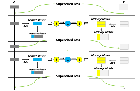
Figure 1: Illustrations of Grug. Considering the messages propagated by the center node (i.e., Node 1), Grug allows to perturb the feature matrix and message matrix, which implements the regularization of gradients on the feature matrix and message matrix.

In this section, we introduce our newly proposed method called Grug, which can be applied to all message-passing HGNNs. We first introduce details of our Grug, and further prove that the most common gradient regularization methods in HGNNs such as random dropping and adversarial perturbations, can be unified into our framework. Then, we present the theoretical evidence of the effectiveness of these methods. Furthermore, we analyze the superiority of Grug, and provide a series of theoretical proofs from the aspects of stability, universality, simplicity and diversity.

4.1 Grug

Algorithm description.

We apply a single RGCN as the backbone model, which can be formulated as $f(F,M,W)=FMW$, where $F\in R^{n\times k}$ denotes the feature matrix, $M$ indicates the message matrix and $W$ denotes the transformation matrix. When we use cross-entropy as the loss function, the objective function can be expressed as follows:

$$L(f(F,M,W),y) =\sum_{i=0}^{K-1}y_{i}\log{(softmax(f(F,M,W)))}$$ (2)

where $K$ is the class number and $y_{i}$ is one hot representation of label $i$.

Different from existing gradient regularization methods, Grug performs gradient regularization both on the feature matrix $F$ and message matrix $M$ instead of either one of them and the process of Grug is in Figure 1. For each element $F_{i,j}$ in $F$ and $M_{i,j}$ in $M$, we generate trained additional elements $\gamma^{i,j}$ and $\delta^{i,j}$ to perturb the original distribution, according to uniform distribution $\gamma^{i,j}\sim Uniform(-\alpha,\alpha)$ and $\delta^{i,j}\sim Uniform(-\beta,\beta)$. After that, we obtain the perturbed $F$ and $M$ by adding each element with its trained additional element. Besides, in the training process, $\gamma^{i,j}$ and $\delta^{i,j}$ can be updated according to the gradient of the previous epoch, which can be expressed as follows:

$$\delta_{t} =\delta_{t-1}+\beta\cdot\frac{\partial_{\delta}L(f(F,M,W),y),y)}{||\partial_{\delta}L(f(F,M,W),y),y)||}$$ (3)

Unifying gradient regularization methods.

In this section, we show that existing gradient regularization methods can be integrated into our Grug. Different from these methods, Grug performs regularization rules on the feature matrix and message matrix. First, we demonstrate that Dropout [34], DropEdge [20], DropNode [21], DropMessage [22] and FLAG [28] can all be formulated as norm regularization process with specific dimension. More importantly, we find that existing methods are a special case of Grug in terms of norm dimensions. In summary, Grug can be expressed as a unified framework of gradient regularization methods on HGNNs.

Theorem 1. Dropout, DropEdge, DropNode, DropMessage and FLAG can be formulated in specific-dimension norm regularization process, and Grug is the generalization case of these methods. We show the regularization term of each method below.

Dropout. dropping the elements $F_{i,j}=\eta F_{i,j}$ where $\eta\sim Bernoulli(\mu)$ is equivalent to perform regularization term $\frac{1}{2}\cdot||\partial_{F_{\zeta}}{L}||_{0}$ on message matrix.

DropEdge. dropping the elements $A_{i,j}=\epsilon A_{i,j}$ where $\epsilon\sim Bernoulli(\mu)$ is equivalent to perform regularization term $\frac{\partial_{A}M}{2}\cdot||\partial_{M_{\epsilon}}{L}||_{0}$ on message matrix.

DropNode. dropping the elements $F_{i}=\eta F_{i}$ where $\zeta\sim Bernoulli(\mu)$ is equivalent to perform regularization term $frac{1}{2}\cdot||\partial_{F_{\zeta}}{L}||_{0}$ on feature matrix.

DropMessage. dropping the elements $M_{i,j}=\tau M_{i,j}$ where $\tau\sim Bernoulli(\mu)$ is equivalent to perform regularization term $\frac{1}{2}\cdot||\partial_{M_{\tau}}{L}||_{0}$ on message matrix.

FLAG. Perturbing the feature matrix $F+\delta$, which is equivalent to perform regularization term $\varepsilon_{t}||\partial_{F}L||_{q_{t}}$ on feature matrix.

Grug. Perturbing both the feature matrix $F+\delta$ and message matrix $M+\xi$, which is equivalent to perform regularization term $\varepsilon_{t}\cdot||\partial_{F}L||_{q_{t}}+\xi_{t}\cdot||\partial_{F}L||_{h_{t}}$ on feature matrix and message matrix. Where $\delta$ and $\gamma$ are the trained $F$ perturbation, which are defined as follows:

$$\delta_{t} =\delta_{t-1}+\beta\cdot\frac{\partial_{\delta}L(f(F+\delta_{t-1},M,W),y)}{||\partial_{\delta}L(f(F+\delta_{t-1},M,W),y)||}$$ (4)

$$\gamma_{t} =\gamma_{t-1}+\alpha\cdot\frac{\partial_{\alpha}L(f(F+\gamma_{t-1},M,W),y)}{||\partial_{\gamma}L(f(F+\gamma_{t-1},M,W),y)||}$$

$||\cdot||_{p_{t}}$ and $||\cdot||_{l_{t}}$ are the dual norm of $||\cdot||_{q_{t}}$ and $||\cdot||_{h_{t}}$, which are defined as follows:

$$||z||_{q} =sup\{z^{T}x\enspace||x||_{p}\leq 1\}\enspace and\enspace\frac{1}{p}+\frac{1}{q}=1$$ (5)

$$||z||_{h} =sup\{z^{T}x\enspace||x||_{l}\leq 1\}\enspace and\enspace\frac{1}{h}+\frac{1}{l}=1$$

We find that the range of regularization dimension of Grug is from $0$ to $\infty$. While for Dropout, DropEdge, DropNode and DropMessage the range of regularization dimension is 0. It is demonstrated that these four methods are special cases of $Grug$. Compared to $FLAG$, $Grug$ can perform different-dimension norm regularization on the feature matrix and message matrix respectively instead of maintaining a consistent-dimension. Thorough proof can be found in Appendix A.1.

4.2 Advantage of Grug.

In this section, we present four further theoretical analyses to elaborate the benefits of Grug from the aspects of stability (decreasing sample variance during the training process), universality(), simplicity (reducing complexity of the model), diversity (improving the integrity and diversity of graph information utilization).

1) Stability.

Existing gradient regularization methods face the problem of sample stability, which is caused by the data noise introduced by different operations, such as dropping and perturbation. Data noise brings the problem of instability in the training process. Generally, sample variance $V$ can be used to measure the degree of stability. A small sample variance means that the training process will be more stable.

Theorem 2. Grug can adjust the sample variance to achieve the stability of the training process.

Intuitively, Grug achieves regularization by adding uniform distribution to the input samples rather than dropping graph data, which means that the sample variance of the input in each epoch is irrelevant to the graph data. In other words, Grug can tune hyperparameters $\alpha$ and $\beta$ to limit the range of sample variance. By reducing the sample variance, Grug diminishes the difference between the feature matrix and message matrix, which stabilizes the training process. Specific range inference can be found in Appendix A.1.

2) Universality.

Theorem 3. Grug performs regularization on the feature matrix and message matrix, which is the optimal general solution compared to existing regularization methods.

As we summarized in Section 2, all existing gradient regularization methods only perform regularization on one of the following three information dimensions, namely node, edge and propagation message. In order to explore which dimension is the optimal solution, we first need to know the relations between these three information dimensions. The relations between these three information dimensions can be expressed as follows:

Regularization on message dimension.

$$\partial_{M}L=\partial_{F}L\cdot\partial_{M}F\quad and\quad\partial_{M}L=\partial_{A}L\cdot\partial_{M}A$$

Regularization on edge dimension.

$$\partial_{A}L=\partial_{M}L\cdot\partial_{A}M\quad and\quad\partial_{A}L=\partial_{F}L\cdot\partial_{M}F\cdot\partial_{A}M$$

Regularization on node dimension.

$$\partial_{F}L=\partial_{M}L\cdot\partial_{F}M\quad and\quad\partial_{F}L=\partial_{A}L\cdot\partial_{M}A\cdot\partial_{F}M$$

The above expressions show that the gradient regularization on each information dimension is transferred to the other two information dimensions. Therefore, regularization on any one information dimension is equivalent to regularization on all three information dimensions theoretically. However, we find that these transfers are not in real-time. Take regularization on the node as an example. In epoch $e_{i}$, the gradient of $F$ can be calculated by $L$, which we express as $\partial_{F}L_{i}$. There is no gradient of $F$ generated from $M$, because the model only keeps the gradient from the loss. However, $\partial_{F}M$ must exist objectively, because $M$ can be seen as a function involving $F$ and $A$. So we can infer that in epoch $e_{i}$, $\partial_{F}M$ is correlated to the previous $e_{i-1}$ epoch. This non-real-time gradient transfer phenomenon is also the same in the edge dimension and message dimension. So we conclude that regularization on only one information dimension cannot apply regularization in real-time to other dimensions. So, gradient regularization on all three information dimensions simultaneously is a better strategy than gradient regularization on one information dimension.

But in practice, we find that compared with node and message dimensions, performing gradient regularization on edge dimension is not only memory consumption, but also reduces the training seed sharply. On the other hand, according to the loss function 2, the node dimension and message dimension, rather than the edge dimension, have the greatest impact on the model loss. Furthermore, performing regularization on the node dimension and message dimension also includes the edge dimension partially. The results of additional experiments show that there are no significant differences between the effects of performing gradient regularization on the edge dimension or not. Therefore, Grug performing regularization on the message and node dimension is the optimal strategy. The Universality is the key for Grug to surpass theoretical upper bounds set by DropMessage and detailed proof are presented in Appendix A.1.

3) Simplicity.

Theorem 4. Message-passing HGNNs using Grug remain one and unique solution, which maintains parameters easily training.

According to Theorem 1 in section 4.1, models using dropping operations on information dimensions can be uniformly expressed as:

$$Drop:\quad\min{||\partial_{X}L||_{0}}\quad and\quad X=F,M,A$$ (6)

$$Gurg:\quad\min{||\partial_{M}L||_{q_{t}}+||\partial_{F}L||_{h_{t}}}$$

Here $||\cdot||_{0}$ represents the 0-dimension Paradigm. However, 0-dimension Paradigm is NP-hardness (non-deterministic polynomial-time hardness) [38] and non-convex [39]. Thus, it is hard to find the solution of functions related to dropping, which makes it hard to run at a satisfactory speed.

In formula (6), the $q_{t}$ and $h_{t}$ are hyperparameters and we can control them by $\alpha$ and $\beta$. So our $Grug$ uses the 1-dimension Paradigm or 2-dimension Paradigm. In theory, the 1-dimension Paradigm [38] and the 2-dimension [40] Paradigm are all convex and remain one and unique solution. Compared to Dropout, DropNode, DropEdge and DropMessage, Grug will not escalate the difficulty of training from the perspective of convexity. The detailed proof is exhibited in Appendix A.1.

4) Diversity.

Theorem 5. Grug is able to maximize the utilization of diverse information in heterogeneous graph.

Utilization of diverse information contains 2 aspects: 1) Obtaining more diverse information 2) Keeping original information diversity.

Obtaining more diverse information is defined as the total number of sample distributions generated during the training process. We propose that the total number of elements in the message matrix is $Z$. For dropping methods, the number of new data distributions is generated by DropMessage, which can be expressed as $C_{Z}^{\frac{Z}{2}}$ and $C$ is a combination in mathematics. Our Grug can continue to generate new data distribution until the end of training.

keeping original information diversity is defined as the total number of preserved feature dimensions. In this term, DropMessage has been proven to perform best in dropping operations. However, Grug seems to lose initial information rarely. This is because perturbation $\delta$ and $\gamma$ will gradually reduce the value of each element as the training progresses. So Grug may lose information only in the initial stage of training.

From the perspective of these 2 aspects, Grug performs better than existing methods. Although Grug may lose some information as other methods, it generates immense new sample distributions, thus maximizing the utilization of diverse information. More details of the derivation are shown in Appendix A.1 and supplementary experiments can be found in Appendix A.3.

5 Experiments

5.1 Experimental Setup

In this section, we present the results of our experiments on five real-world datasets for node classification and link prediction tasks. Our experiments aim to answer the following questions: 1) How does Grug compare to other gradient regularization methods on HGNNs in terms of performance? 2) Can Grug improve the robustness of HGNNs? 3) Does Grug perform better than other methods in addressing over-smoothing problems?

Datasets We employ five commonly used heterogeneous graph datasets in our experiments, which are ACM, DBLP, IMDB, Amazon and LastFM.

Node Classification Datasets. Labels in node classification datasets are split according to 20% for training, 10% for validation and 70% for test in each dataset. Note that node classification datasets are the same version used in the GTN [41].

• ACM is a paper citation network, containing 3 types of nodes (papers (P), authors (A), subjects (S)), 4 types of edges (PS, SP, PA, AP).

• DBLP is a bibliography website of computer science. It contains 3 types of nodes (papers (P), authors (A), conferences (C)), 4 types of edges (PA, AP, PC, CP).

• IMDB is a website about movies and related information. It contains 3 types of nodes (movies (M), actors (A), and directors (D)) and labels are genres of movies.

Link Prediction Datasets. Edges in link prediction datasets are split according to 25% for training, 5% for validation and 60% for the test in each dataset. Note that link prediction datasets are subsets pre-processed by HGB dataset [11].

• Amazon is an online purchasing platform and it consists of electronics products with co-viewing and co-purchasing links between them.

• LastFM is an online music website. It contains 3 types of nodes (artist, user, tag) and 3 types of edges (artist-tag, user-artist, user-user).

Baseline methods. We compare our proposed Grug with other existing gradient regularization methods, including Dropout (2012) [19], DropNode (2020) [21], DropMessage (2022) [22], and FLAG (2020) [28]. We adopt these methods on backbone models and compare their performances on different datasets.

Backbone models. In order to compare the differences of gradient regularization methods fairly, we choose the basic HGNN models to ensure that the experimental results are not affected by the difference of the models. So we consider two mainstream HGNNs as our backbone models: RGCN [4] and RGAT [5]. We implement the gradient regularization methods mentioned above on backbone models.

Dataset		ACM		DBLP		IMDB
Method		Macro F1	Macro F1	Micro F1	Macro F1	Micro F1	Macro F1
RGCN	Clean [4]	90.36±0.60	90.44±0.59	93.67±0.15	92.77±0.16	56.05±1.84	55.43±1.64
	Dropout [19]	90.86±0.39	90.91±0.40	94.35±0.14	93.53±0.14	57.63±1.01	56.04±0.79
	DropNode [21]	90.68±0.75	90.74±0.77	93.85±0.71	93.12±0.71	57.38±0.37	56.20±0.50
	DropMessage [22]	91.57±0.19	91.57±0.21	94.69±0.13	93.96±0.13	57.60±0.84	56.48±0.49
	FLAG [28]	92.43±0.37	92.58±0.34	94.22±0.20	93.39±0.24	56.74±0.33	55.63±0.40
	Grug	93.27±0.13	93.33±0.13	95.08±0.08	94.17±0.11	59.92±0.56	58.87±0.71
RGAT	Clean [4]	89.32±1.03	89.34±1.03	92.98±0.61	92.15±0.63	53.12±0.80	52.75±0.78
	Dropout [19]	89.38±0.81	89.51±0.76	93.55±0.48	92.69±0.50	54.85±0.31	53.63±0.26
	DropNode [21]	89.86±0.67	89.98±0.60	93.21±0.67	92.42±0.72	53.86±1.56	52.80±1.60
	DropMessage [22]	90.57±0.62	90.57±0.62	93.89±0.35	93.01±0.39	56.48±0.76	55.29±0.78
	FLAG [28]	91.46±0.59	91.53±0.58	93.38±0.45	92.42±0.35	56.09±0.68	54.47±0.66
	Grug	92.84±0.18	92.92±0.19	94.21±0.21	93.50±0.22	57.79±0.37	56.17±0.18

Table 1: Comparison results of different gradient regularization methods for node classification. The best results are in bold.

5.2 Comparison Results

Table 2 and Table 1 summarize the overall results. For node classification tasks, we employ the Micro F1 score and Macro F1 score as Metrics on 3 datasets (ACM, DBLP, IMDB). For link prediction tasks, the performance is measured by AUC-ROC on Amazon and LastFM. Considering the space limitation, some additional experiments are presented in the Appendix A.3.

Dataset		Amazon	LastFM
Method		AUC-ROC	AUC-ROC
RGCN	Clean [4]	70.54±5.00	56.66±5.92
	Dropout [19]	72.83±5.17	56.95±2.37
	DropNode [21]	70.81±3.85	56.97±3.86
	DropMessage [22]	81.80±0.57	58.01±4.65
	FLAG [28]	78.87±0.81	56.96±4.32
	Grug	80.93±0.67	60.37±1.24
RGAT	Clean[4]	81.98±2.36	78.09±3.97
	Dropout [19]	81.74±6.72	78.94±3.43
	DropNode [21]	83.36±0.77	78.10±2.85
	DropMessage [22]	85.16±0.35	78.50±0.52
	FLAG [28]	85.59±0.25	78.66±1.86
	Grug	86.84±0.26	80.39±2.24

Table 2: Comparison results of different gradient regularization methods for link prediction. The best results are in bold.

Overall, Grug performs well in all scenarios (node classification and link prediction), indicating its stability in diverse situations. For node classification tasks, we have 72 settings, each of which is a combination of different backbone models and datasets in different metrics (e.g., RGCN-ACM-Macro F1). Table 1 shows that Grug achieves the optimal results in all 72 settings. As to 24 settings under the link prediction task, Grug achieves the optimal results in 23 settings, and sub-optimal results in 1 setting. Besides, Grug performs more stable on all datasets and all tasks than other methods clearly. Taking Dropout as the counterexample, it appears strong performance on the DBLP dataset but shows a clear decrease on the ACM dataset and IMDB dataset. In terms of tasks, the performance of Dropout on link prediction is far worse than that on node classification. Dropout on node classification obtains an average accuracy decline of 2.97% compared to Grug. This numerical gap has widened to 7.69% on link prediction. A reasonable explanation is that the information dimensions operated by distinct methods vary from each other as shown in section 4.2. With the generalization of its operation on node and message dimensions, DropMessage obtains a smaller inductive bias. Therefore, Grug is more applicable for most scenarios.

5.3 Additional Results

Over Smoothing analysis. In this section, we investigate the issue of over-smoothing in HGNNs, which occurs when node representations become indistinguishable as the depth of the network increases, leading to poor results. To address this problem, we compare the effectiveness of different gradient regularization methods, taking into account the information diversity discussed in Section 4.2. As mentioned in section 4.2, Grug obtaining more diverse information in the training process, it is expected to perform better holdout over-smoothing in theory. To verify this, we conduct experiments on two datasets, ACM and IMDB, using RGCN as the backbone model. As Figure 2 suggests, we can find that all gradient regularization methods can alleviate over-smoothing and Grug) outperforming other methods due to their diverse information. Our proposed Grug exhibits consistent superiority in performance across all layers (from layer 1 to layer 7), as shown in Figure 2.

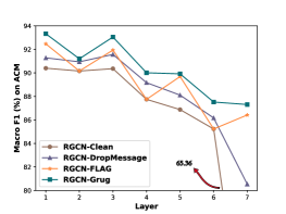
(a) ACM

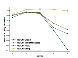
(b) IMDB

Figure 2: Over-Smoothing Analysis.

Robustness analysis. We evaluate the robustness of different gradient regularization methods by measuring their ability to deal with perturbed heterogeneous graphs. In more detail, we randomly add a certain ratio of edges on ACM and DBLP datasets and address the node classification task. It is found in Figure 3 that Grug has positive effects and results drop the least when the perturbation rate increase from 0.1 to 0.4. Besides, our proposed Grug shows its stability and outperforms other gradient regularization methods in noisy situations.

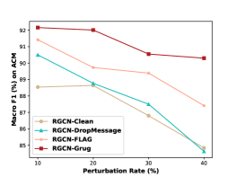
(a) ACM

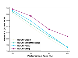
(b) DBLP

Figure 3: Model Performances Against Attacks.

6 Conclusion

In this paper, we propose Grug, a general and effective gradient regularization method for HGNNs. We first unify existing gradient regularization methods to our framework via performing regularization according to the gradient on the feature matrix and message matrix. As Grug operates meticulously on feature and message matrix, it is a generalization of existing methods, which shows greater applicability in general cases. Besides, we provide the theoretical analysis of the superiority (stability, simplicity and diversity) and effectiveness of Grug. By conducting sufficient experiments for multiple tasks on five datasets, we show that Grug surpasses the SOTA performance and alleviates over-smoothing, and non-robustness obviously compared to the traditional gradient regularization methods.

Appendix A Appendix

A.1 Derivation Details.

Detailed proof of Theorem 1.

Theorem 1 Dropout, DropEdge, DropNode, DropMessag and FLAG can be formulated specific-dimension norm regularization process and Grug is the generalization case of these methods.

We present more derivation details of Theorem 1. Here we use cross entropy $L$ as the basis loss function, and the objective function $L^{\sim}$ for each method in expectation can be expressed as follows:

Dropout:

$$E(L^{\sim}) =E(L^{\sim}(f(F,M_{\eta},W),y))$$

$$\approx E(L^{\sim}(f(F,M_{\eta},W),y))+\frac{1}{2}\cdot\partial_{M}L(f(F,M_{\eta},W),y)$$

$$\approx L+\frac{1}{2}\cdot\frac{\partial L}{\partial{M_{\eta}}}\cdot\frac{\partial{M_{\eta}}}{\partial{M}}$$

$$\approx L+\frac{1}{2}\cdot||\partial_{M_{\eta}}{L}||_{0}$$

where $\eta\sim Bernoulli(\mu)$ and $M_{\eta}$ is the dropped $M$. Note that $F_{i,j}=\eta F_{i,j}$ which means that $\mu$ elements of $F$ can be dropped in expectation.

DropEdge: As objective function $L^{\sim}$ does not explicitly include $A$, so we use the following inference to convert dropping on $A$ to dropping on $M$:

$$\partial_{A}L=\frac{\partial L}{\partial M}\cdot\frac{\partial M}{\partial A}=\partial_{M}L\cdot\partial_{A}M$$

Therefore, the objective function for DropEdge can be expressed as follows:

$$E(L^{\sim}) \approx E(L^{\sim}(f(F,M_{\epsilon},W),y))+\frac{1}{2}\cdot\partial_{M}L(f(F,M_{\epsilon},W),y)\cdot\partial_{A}M$$

$$\approx L+\frac{1}{2}\cdot\frac{\partial L}{\partial{M_{\epsilon}}}\cdot\frac{\partial{M_{\epsilon}}}{\partial{M}}\cdot\partial_{A}M$$

$$\approx L+\frac{\partial_{A}M}{2}\cdot||\partial_{M_{\epsilon}}{L}||_{0}$$

where $\epsilon\sim Bernoulli(\mu)$ and $M_{\epsilon}$ is the dropped $M$. Note that $A_{i,j}=\epsilon A_{i,j}$ which means that $\mu$ elements of $A$ and $\mu$ columns of $M$ will be dropped in expectation.

DropNode:

$$E(L^{\sim}) =E(L^{\sim}(f(F_{\zeta},M,W),y))$$

$$\approx E(L^{\sim}(f(F_{\zeta},M,W),y))+\frac{1}{2}\cdot\partial_{F}L(f(F_{\zeta},M,W),y)$$

$$\approx L+\frac{1}{2}\cdot\frac{\partial L}{\partial{F_{\zeta}}}\cdot\frac{\partial{F_{\zeta}}}{\partial{F}}$$

$$\approx L+\frac{1}{2}\cdot||\partial_{F_{\zeta}}{L}||_{0}$$

where $\zeta\sim Bernoulli(\mu)$ and $F_{\zeta}$ is the dropped $F$. Note that $F_{i}=\eta F_{i}$ which means that $\mu$ rows of $F$ will be dropped in expectation.

DropMessage:

$$E(L^{\sim}) =E(L^{\sim}(f(F,M_{\tau},W),y))$$

$$\approx E(L^{\sim}(f(F,M_{\tau},W),y))+\frac{1}{2}\cdot\partial_{M}L(f(F,M_{\tau},W),y)$$

$$\approx L+\frac{1}{2}\cdot\frac{\partial L}{\partial{M_{\tau}}}\cdot\frac{\partial{M_{\tau}}}{\partial{M}}$$

$$\approx L+\frac{1}{2}\cdot||\partial_{M_{\tau}}{L}||_{0}$$

where $\tau\sim Bernoulli(\mu)$ and $M_{\tau}$ is the dropped $M$. Note that $M_{i,j}=\tau M_{i,j}$ which means that $\mu$ elements of $M$ will be dropped in expectation.

FLAG:

Note that in each epoch, FLAG train parameters $N$ times, and scale the gradient to $\frac{1}{N}$ of the true gradient for accumulation, and update the perturbation $N-1$ times in the process of accumulating the gradient, which is adopted in Grug.

$$E(L^{\sim}) =\frac{1}{N}\sum_{t=0}^{N-1}{E(L^{\sim}(f(F+\delta_{t},M,W),y))}$$

$$\approx\frac{1}{N}\sum_{t=0}^{N-1}E(L^{\sim}(f(F,M,W),y)))+\frac{1}{N}\sum_{t=0}^{N-1}\frac{\delta_{t}}{2}\partial_{F}L^{\sim}(f(F,M,W),y)$$

$$=L+\frac{1}{N}\sum_{t=0}^{N-1}\frac{1}{2}\cdot\max_{\delta_{t}:\left\|\delta_{t}\right\|_{p}\leq\varepsilon_{t}}{|L(f(F+\delta_{t},M,W),y)-L(f(F,M,W),y)|}$$

$$\approx L+\frac{1}{2N}\sum_{t=0}^{N-1}\cdot\max_{\delta_{t}:\left\|\delta_{t}\right\|_{p}\leq\varepsilon_{t}}{\delta_{t}\cdot\partial_{F}L}$$

$$=L+\frac{1}{2N}\sum_{t=0}^{N-1}\varepsilon_{t}||\partial_{F}L||_{q_{t}}$$

where the perturbation $\delta$ iteratively updates N times in each epoch. We can approximate the loss function with the second-order Taylor expansion of $f(\cdot)$ around $\delta$. Thus, the objective loss function in expectation can be expressed as below:

$$\delta_{t} =\delta_{t-1}+\beta\cdot\frac{\partial_{\delta}L(f(F+\delta_{t-1},M,W),y)}{||\partial_{\delta}L(f(F+\delta_{t-1},M,W),y)||}$$

and $||\cdot||_{p_{t}}$ is the dual norm of $||\cdot||_{q_{t}}$,which is defined as follows:

$$||z||_{q} =sup\{z^{T}x\enspace||x||_{p}\leq 1\}\enspace and\enspace\frac{1}{p}+\frac{1}{q}=1$$

Grug:

$$E(L^{\sim}) =E(\frac{1}{N}\sum_{t=0}^{N-1}L^{\sim}(f(F+\delta_{t},M+\gamma_{t},W),y))$$

$$\approx{\frac{1}{N}\sum_{t=0}^{N-1}L(f(F+\delta_{t},M,W),y)+\frac{1}{N}\sum_{t=0}^{N-1}\frac{\gamma_{t}}{2}\cdot\partial_{M}L(f(F+\delta_{t},M,W),y)}$$

$$\approx{L(f(A,M,W),y)+\frac{1}{N}\sum_{t=0}^{N-1}\frac{\delta_{t}}{2}\cdot\partial_{F}L(f(F,M,W),y)}+$$

$$\frac{1}{N}\sum_{t=0}^{N-1}\frac{\gamma_{t}}{2}\cdot\partial_{M}(L(f(F,M,W),y)+\frac{\delta_{t}}{2}\cdot\partial_{F}L(f(F,M,W),y))$$

$$=L+\frac{1}{N}\sum_{t=0}^{N-1}\frac{\delta_{t}}{2}\cdot\partial_{F}L+\frac{1}{N}\sum_{t=0}^{N-1}\frac{\gamma_{t}}{2}\cdot\partial_{M}L+\frac{1}{N}\sum_{t=0}^{N-1}\frac{\gamma_{t}}{2}\cdot\frac{\delta_{t}}{2}\cdot\partial_{F}(\partial_{M}L)$$

$$\approx L+\frac{1}{2N}\sum_{t=0}^{N-1}\varepsilon_{t}\cdot||\partial_{F}L||_{q_{t}}+\frac{1}{2N}\sum_{t=0}^{N-1}\xi_{t}\cdot||\partial_{F}L||_{h_{t}}$$

where $\delta$ and $\gamma$ are the trained $F$ perturbation, which are defined as follows:

$$\delta_{t} =\delta_{t-1}+\beta\cdot\frac{\partial_{\delta}L(f(F+\delta_{t-1},M,W),y)}{||\partial_{\delta}L(f(F+\delta_{t-1},M,W),y)||}$$

$$\gamma_{t} =\gamma_{t-1}+\alpha\cdot\frac{\partial_{\alpha}L(f(F+\gamma_{t-1},M,W),y)}{||\partial_{\gamma}L(f(F+\gamma_{t-1},M,W),y)||}$$

$||\cdot||_{p_{t}}$ and $||\cdot||_{l_{t}}$ are the dual norm of $||\cdot||_{q_{t}}$ and $||\cdot||_{h_{t}}$,which are defined as follows:

$$||z||_{q} =sup\{z^{T}x\enspace||x||_{p}\leq 1\}\enspace and\enspace\frac{1}{p}+\frac{1}{q}=1$$

$$||z||_{h} =sup\{z^{T}x\enspace||x||_{l}\leq 1\}\enspace and\enspace\frac{1}{h}+\frac{1}{l}=1$$

Detailed proof of Theorem 2.

Theorem 2 Grug can adjust the sample variance to achieve the stability of the training process .

In order to make the conclusion more general, we assume the original $M$ is $1_{n\times n}$, which means that every element in $M$ is $1$.Thus, we can calculate its sample variance via the 1-norm of the $M$.

The sample variance of FLAG can be expressed as follows:

$$V(|FLAG|) =V(M+\gamma_{t})-V(M+\gamma_{t-1})$$

$$=V(\gamma_{t}-\gamma_{t-1})$$

$$=V(\alpha\cdot\textbf{A})$$

$$=\alpha^{2}V(\textbf{A})$$

where A is a distribution containing only 1 and -1, so the range of $A$ variance is from 0 to 1. So the range of FLAG variance can be calculated as follows:

$$0\leq V(FLAG)\leq\alpha^{2}$$

Similarly, we can calculate range of Grug variance as follows:

$$0\leq V(\textit{Grug})\leq\alpha^{2}+\beta^{2}$$

DropMessage has been proven to have the smallest sample variance among random dropping methods, which can be expressed as follows:

$$\ V(|DropMessage|) =V(M_{\eta})-V(M_{\eta^{\sim}})$$ (7)

$$=V(M\times\textbf{R})$$

$$=V(M)\cdot V(\textbf{R})+V(M)\cdot E(\textbf{R})^{2}+V(\textbf{R})\cdot E(M)^{2}$$

where R is a distribution containing 1, 0 and -1, so the range of its expectations is from 0 to 1 and the range of its variance is from 0 to 1 too. So we calculate the range of DropMessage as follows:

$$0\leq V(|DropMessage|)\leq 2V(M)+E(M)^{2}$$

Detailed proof of Theorem 3.

Theorem 3 Grug perform regularization on 2 information dimension, namely feature and message, which is the optimal solution of existing regularization methods.

When we perform regularization on the adjacency matrix, the regularization term must contain $\partial_{A}L$. We can map this term to $\partial_{M}L$, which can be expressed as:

$$\partial_{A}L=\frac{\partial L}{\partial M}\cdot\frac{\partial M}{\partial A}=\partial_{M}L\cdot\partial_{A}M$$

where $\partial_{A}M$ is a function involving $\partial_{F}$.

Similarly, we can express regularization terms on the feature matrix as:

$$\partial_{F}L=\frac{\partial L}{\partial M}\cdot\frac{\partial M}{\partial F}=\partial_{M}L\cdot\partial_{F}M$$

where $\partial_{f}M$ is a function involving $\partial_{A}$.

For regularization $\partial_{M}L$ on the message matrix, there are two inferences as follows:

$$\partial_{M}L=\frac{\partial L}{\partial F}\cdot\frac{\partial F}{\partial M}=\partial_{F}L\cdot\partial_{M}F$$

$$\partial_{M}L=\frac{\partial L}{\partial A}\cdot\frac{\partial A}{\partial M}=\partial_{A}L\cdot\partial_{M}A$$

Here we take the regularization of node dimension as an example. When we only apply regularization on the message dimension, the regularization on the node dimension can be expressed as:

$$\partial_{F}L=\frac{\partial L}{\partial M}\cdot\frac{\partial M}{\partial F}=\partial_{M}L\cdot\partial_{F}M$$

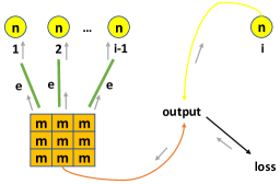
Figure 4: Process of gradient generation for node $i$.

Figure 4 shows the process of gradient generation for node $i$. We find that regularization on dimensions is convertible, which means that when performing regularization on one dimension, it may also apply regularization in other dimensions at the same time (in one epoch). More specifically, the conversion is as follows:

• Node: nodes.

• Message: message, edges and a part of nodes.

• Edge: edges and a part of nodes.

So in one epoch, in order to apply regularization on all dimensions, the optimal method is performing regularization on the message dimension and node dimension. In order to make our inferences interpretable, we take performing regularization on message dimension as an example.

Definition 1 For $\partial_{F}M_{i,j}$ in $\partial_{F}M$, it can be expressed as partial derivative of $M_{j}$ to $F_{i}$ and its value is 0 if $M_{j}$ is not generated by $F_{i}$

$$\begin{bmatrix}\partial_{x_{1}}m_{1}\quad\partial_{x_{2}}m_{1}\quad\dots\quad\partial_{x_{p}}m_{1}\\ \partial_{x_{1}}m_{2}\quad\partial_{x_{2}}m_{2}\quad\dots\quad\partial_{x_{p}}m_{2}\\ \dots\quad\dots\quad\dots\quad\dots\\ \partial_{x_{1}}m_{k}\quad\partial_{x_{2}}m_{k}\quad\dots\quad\partial_{x_{p}}m_{k}\end{bmatrix}$$

In the training process of node $n_{i}$ in one epoch $e_{k}$, node $n_{i}$ receives message $m_{i}$ from neighbor nodes ($n_{1}$, $n_{2}$ … $n_{i-1}$). Performing regularization on message $m_{i}$, according to Chain rule (Rule of composed derivatives), is equivalent to performing regularization on $n_{1}$, $n_{2}$ … $n_{i-1}$ without $n_{i}$ in a certain rule. However, in next epoch $e_{i+1}$, regularization on message $m_{i}$ can convert to node $n_{i}$, which can be expressed as follows:

$$M_{i+1} =M_{i}-\psi\cdot reg(\partial_{M_{i}}L_{i})$$

$$F_{i+1} =F_{i}-\psi\cdot\partial_{F_{i}}L_{i}$$

$$\partial_{F_{i+1}}L_{i+1} =\frac{\partial((F_{i}-\psi\cdot\partial_{F_{i}}L_{i})\cdot(M_{i}-\psi\cdot reg(\partial_{M_{i}}L_{i}))\cdot W)}{\partial(F_{i}-\psi\cdot\partial_{F_{i}}L_{i})}$$

Despite regularization on $m_{i}$ can convert to $n_{i}$ in the training process with the epochs increasing. This conversion is noninterpretable and uncontrollable.

Detailed proof of Theorem 4.

Theorem 4 Message-passing HGNNs using Grug remain one and unique solution, which maintains parameters easily training.

In fact, the concavity and convexity of the function will directly affect the convergence rate of the parameters. Here we express $Grug$ (convex) as $F(x)$. So we can get the proportional relationship of the difference of the objective function between any 2 epochs $i$ and $*$.

$$F(x_{i})-F(x_{*}) \leq F(x_{i-1})-F(x_{*})-\psi\cdot||\bigtriangledown F(x_{i-1})||^{2}$$

$$\leq F(x_{i-1})-F(x_{*})-\frac{\psi}{\omega}(F(x_{i-1})-F(x_{*}))$$

$$=(1-\frac{\psi}{\omega})(F(x_{i-1})-F(x_{*}))$$

where $F(x_{i})-F(x_{i-1})\geq\omega||\bigtriangledown f(x_{i-1})||^{2}$ as $F(x)$ is convex. So when objective function $F(x)$ reach the least deviation $\vartheta$ in final epoch $T$, the inference is as follows:

$$F(x_{T})-F(x_{*}) \leq\vartheta$$

$$(1-\frac{\psi}{\omega})^{T}(F(x_{0})-F(x_{*})) \leq\vartheta$$

$$\frac{1}{(1-\frac{\psi}{\omega})^{T}(F(x_{0})-F(x_{*}))} \geq\frac{1}{\vartheta}$$

$$T \geq\frac{\frac{(F(x_{0})-F(x_{*}))}{\vartheta}}{\log\frac{1}{(1-\frac{\psi}{\omega})}}$$

So $T$ in $Grug$ function $F(x)$ is $O(\log\frac{1}{\vartheta})$ order.

For drop methods (non-convex), objective functions $F(x)$ is non-convex. When it converges, its first-order gradient satisfies as follows:

$$\bigtriangledown||F(x_{i})||\leq\vartheta$$

So in final epoch $T$, $F_{x_{T}}$ can be expressed:

$$F(x_{T}) \leq F(x_{0})-\psi\sum_{i=0}^{T-1}||\bigtriangledown F(x_{T-1})||^{2}$$

$$\psi\sum_{i=0}^{T-1}||\bigtriangledown F(x_{T-1})||^{2} \leq F(x_{0})-F(x_{T})\leq F(x_{0})-F(x_{*})$$

$$\min||\bigtriangledown F(x_{T-1})||^{2} \leq||\bigtriangledown F(x_{T-1})||^{2}\leq\frac{F(x_{0})-F(x_{*})}{\psi T}$$

$$||\bigtriangledown F(x_{T-1})||^{2} \leq O(\frac{1}{T})\leq\vartheta^{2}$$

So $T$ in drop method function $F(x)$ is $O(\frac{1}{\vartheta^{2}})$ and it is easy to find that $O(\frac{1}{\vartheta^{2}})>O(\log\frac{1}{\vartheta})$. So compared to drop methods, $Grug$ needs fewer epochs to reach convergence.

Detailed proof of Theorem 5.

Theorem 5 Grug is able to maximize the utilization of diverse information in heterogeneous graph.

Since DropMessage has been proven to be the most capable of keeping diverse information in the drop method, we compare 3 methods: DropMessage, FLAG, Grug.

1) More diverse information.

For each element $m_{i,j}$ in message matrix $M$, $m_{i,j}^{\sim}$ represents the information actually used in epoch $e_{k}$. In epoch $e_{k}$, $m_{i,j}^{\sim}$ can be expressed as follows:

DropMessage:

$$m_{i,j}^{\sim}=m_{i,j}\quad or\quad 0$$

FLAG/Grug:

$$m_{i,j}^{\sim}=m_{i,j}+\gamma_{i,j}^{0}+\sum_{k=0}^{s-1}\psi\cdot\partial_{\gamma_{i,j}^{k}}L_{k}$$

where $r_{0}$ represents the initial value of $\gamma$, and $\psi$ represents the learning ratio for the training process. The $s$ is the total number of epochs, and $k$ is the current training epoch. Here we use $L_{k}$ to represent the loss of the $kth$ epoch. The derivation of Grug can be found in section 4.1.

During the training process, the $L_{k}$ reduces gradually in each epoch, so the $\partial_{\gamma_{i,j}^{k}}L_{k}$ also decreases in each epoch. The value of $m_{i,j}^{\sim}$ is updated $s$ times, which means that $m_{i,j}^{\sim}$ does not generate duplicate values in the $s$ times. Therefore, the $m_{i,j}^{\sim}$ of FLAG and Grug is higher than the $m_{i,j}^{\sim}$ of DropMessage.

For the FLAG, it only performs regularization on the node dimension without considering the message dimension. This must result in generating duplicate values in $m_{i,j}^{\sim}$ because several messages may come from the same node. Here $Q()$ represents the amount of $m_{i,j}^{\sim}$ in the training process. So the $Q()$ of Grug, FLAG and DropMessage can be expressed as follows:

$$Q(Grug)>Q(FLAG)>Q(DropMessage)$$

2) Retain original information.

Additional experiments A.3 show that drop methods have the risk of over-fitting. We hypothesize that one of the causes of overfitting is the loss of original information. Here we theoretically analyze the ability to retain original information between the drop methods and Grug. For the DropMessage, if the drop ratio is $\chi$, the information loss ratio of DropMessage is also $\chi$.

For FLAG and $Grug$, we assume that $m_{i,j}$ loses $d_{i,j}$ information in epoch $e_{k}$, which can be expressed as:

$$d_{i,j} =(m_{i,j}+\alpha\frac{\partial_{m_{i,j}}L}{|\partial_{m_{i,j}}L|}-m_{i,j})/m_{i,j}$$

$$=\alpha\frac{\partial_{m_{i,j}}L}{|\partial_{m_{i,j}}L|})/m_{i,j}$$

$$\propto\partial_{m_{i,j}}L$$

The value of $d_{i,j}$ depends on $\partial_{m_{i,j}}L$. Besides, during the training processing, $d_{i,j}$ gradually decreases to 0 as gradient $\partial_{m_{i,j}}L$ gradually declines to 0. In summary, the ratio of loss information can be found as follows:

$$Grug,FLAG<DropMessage$$

A.2 Experiment Details

Dataset	Heterogeneous Nodes	Heterogeneous Edges	Features
ACM	5912/3025/57	9936/3025	1902
DBLP	4057/14328/20/8789	19645/14328/88420	334
IMDB	4661/5841/2270	13983/4661	1256
amazon	10099	76924/71735	1156
LastFM	1892/17632/1088	92834/25434/23523	0

Table 3: Dataset Statistics.

Hardware specification and environment. We run our experiments on the machine with 12th Gem Inter(R) Core(TM) (2.70 GHz), NVIDIA RTX 3050 GPUs (16 GB). The code is written in Python 3.9 and Pytorch 1.12.1.

Dataset statistics. Table 3 shows the statistics of datasets.

Dataset	$\alpha$	$\beta$
RGCN-ACM	0.35	0.01
RGAT-ACM	0.08	0.01
RGCN-DBLP	0.11	0.01
RGAT-DBLP	0.0001	0.001
RGCN-IMDB	0.002	0.0001
RGAT-IMDB	0.001	0.0004

Table 4: Statistics of Optimal $\alpha$ and $\beta$ for Node Classification.

Dataset	$\alpha$	$\beta$
RGCN-amazon	0.0002	0.0001
RGAT-amazon	0.003	0.001
RGCN-LastFM	0.002	0.001
RGAT-LastFM	0.001	0.002

Table 5: Statistics of Optimal $\alpha$ and $\beta$ for Link prediction.

Implementation details. We conduct 10 independent experiments for each setting and obtain the average results. We apply 1-layer models to the three datasets of node prediction tasks (ACM, DBLP, IMDB). However, for the datasets of link prediction tasks (amazon, LastFM), we use three-layer models. In all cases, we use the Adam optimizer with learning rate of 0.001 and train each model 200 epochs. We adjust the $\alpha$ and $\beta$ from 0.0001 to 0.5 in steps of 0.0001 and select the optimal one for each setting. Table 4 and 5 present the optimal parameter we selected.

A.3 Additional Experiments

In section 4.2, we present that Grug can directly control the sample variance to maintain the stability of the training process. We conduct experiments and record training loss and validation loss fluctuation throughout the whole training process. Figure 5 shows the change of loss in RGCN training processes when employing different gradient regularization methods on the ACM dataset. We have the following observations:

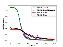
(a) Training Process

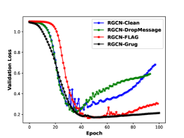
(b) Validation Process

Figure 5: Training Process and Validation Process Analysis.

Training process analysis.

1) In training process, loss of Grug declines more stability than DropMessage.

2) In the validation process, the performance of Grug keeps stable while other methods suffer from over-fitting.

3) DropMessage quickly reach convergence (around epoch 50), but the problem of over-fitting for it compares to Grug.

Observation 1 presents the stability of Grug, which is consistent with the theoretical results in Section 4.2. Observation 2 suggests that Grug receives more diverse information than other methods. Observation 3 indicates that Grug keeps the original information while DropMessage is not. This verifies our theory in section 4.2. In conclusion, taking Grug as the gradient regularization method can obtain more diverse information and stability in the face of over-fitting problems.

Ablation experiments

The ablation studies on all the five datasets are summarized in Table 6. We conduct 4 ablation regularization methods as a comparison.

• $Grug_{n}:$ only performs regularization on the node dimension.

• $Grug_{e}:$ only performs regularization on the edge dimension.

• $Grug_{m}:$ only performs regularization on the message dimension.

• $Grug_{T}:$ performs regularization on the message dimension, node dimension and edge dimension.

Task		Node Classification			Link prediction
Dataset		ACM	DBLP	IMDB	amazon	LastFM
RGCN	$Grug_{n}$	92.43	94.22	56.74	78.87	56.96
	$Grug_{e}$	91.08	93.97	56.55	77.32	55.92
	$Grug_{m}$	91.22	94.47	56.99	78.56	56.89
	$Grug_{T}$	93.30	95.05	60.05	80.99	60.56
	$Grug$	93.27	95.08	59.92	80.93	60.37
	$GAP$	-0.03	+0.03	-0.13	-0.06	-0.19
RGAT	$Grug_{n}$	91.46	93.38	56.09	85.59	78.66
	$Grug_{e}$	90.56	93.45	56.98	83.11	77.65
	$Grug_{m}$	90.97	93.94	57.37	84.97	78.95
	$Grug_{T}$	92.90	94.01	57.88	86.67	80.37
	$Grug$	92.84	94.21	57.79	86.84	80.39
	$GAP$	-0.06	+0.20	-0.09	+0.17	+0.02

Table 6: Ablation results.

In section 4.2, we suggest performing regularization on the message dimension and node dimension as a selection without considering on edge dimension. Table 6 shows the gap between $Grug_{T}$ and $Grug$. The average gap is only 0.013 for node classification and 0.015 for link prediction. Besides, performing regularization on edge dimensions needs to generate a new adjacency matrix in each epoch, which consumes extra time and memory. So Grug choose message dimension and node dimension as a substitute for all dimensions. On the other hand, in 10 settings, $Grug_{m}$ and $Grug_{n}$ achieve the optimal results in 5 settings and 5 settings respectively. However, $Grug_{e}$ performs not well as the other 2 methods. In conclusion, Grug performing regularization on the message and node dimension is the optimal strategy.

Gradient Norm Analysis.

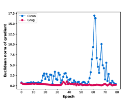
(a) Euclidean norm (L2 norm)

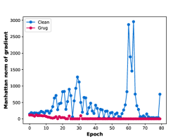
(b) Manhattan norm (L1 norm)

Figure 6: Paradigm norm of gradient analysis.

As we mentioned in section 4.2, the 1-dimension Paradigm norm and 2-dimension Paradigm norm can be regarded as a specific form of Grug. Figure 6 shows the Euclidean norm and Manhattan norm of the gradient in the training process. We find that using Grug can make the 1-dimension Paradigm and 2-dimension Paradigm small in the whole training process. Figure 6(a) shows the Euclidean norm between model and mode using Grug, suggesting that Grug performs better in narrowing the 2-dimension Paradigm of the gradient. Besides Figure 6(b) indicates that Grug can also limit the value of the 1-dimension Paradigm of the gradient. Therefore, compared with previous methods, the gradient of Grug can remain stable in the training process without great fluctuation. A smoother gradient generated by Grug can significantly improve the speed and efficiency of training convergence of the model. This experimental result is consistent with the theoretical proof of section 4.2.

References

- [1] Peter W Battaglia, Jessica B Hamrick, Victor Bapst, Alvaro Sanchez-Gonzalez, Vinicius Zambaldi, Mateusz Malinowski, Andrea Tacchetti, David Raposo, Adam Santoro, Ryan Faulkner, et al. Relational inductive biases, deep learning, and graph networks. arXiv preprint arXiv:1806.01261, 2018.
- [2] Thomas N Kipf and Max Welling. Semi-supervised classification with graph convolutional networks. arXiv preprint arXiv:1609.02907, 2016.
- [3] Yuxiao Dong, Nitesh V Chawla, and Ananthram Swami. metapath2vec: Scalable representation learning for heterogeneous networks. In Proceedings of the 23rd ACM SIGKDD international conference on knowledge discovery and data mining, pages 135–144, 2017.
- [4] Michael Schlichtkrull, Thomas N Kipf, Peter Bloem, Rianne Van Den Berg, Ivan Titov, and Max Welling. Modeling relational data with graph convolutional networks. In The Semantic Web: 15th International Conference, ESWC 2018, Heraklion, Crete, Greece, June 3–7, 2018, Proceedings 15, pages 593–607. Springer, 2018.
- [5] Kai Wang, Weizhou Shen, Yunyi Yang, Xiaojun Quan, and Rui Wang. Relational graph attention network for aspect-based sentiment analysis. arXiv preprint arXiv:2004.12362, 2020.
- [6] Massimo Quadrana, Paolo Cremonesi, and Dietmar Jannach. Sequence-aware recommender systems. ACM Computing Surveys (CSUR), 51(4):1–36, 2018.
- [7] Yi Tay, Anh Tuan Luu, and Siu Cheung Hui. Multi-pointer co-attention networks for recommendation. In Proceedings of the 24th ACM SIGKDD international conference on knowledge discovery & data mining, pages 2309–2318, 2018.
- [8] Ziniu Hu, Yuxiao Dong, Kuansan Wang, and Yizhou Sun. Heterogeneous graph transformer. In Proceedings of the web conference 2020, pages 2704–2710, 2020.
- [9] Xiao Wang, Houye Ji, Chuan Shi, Bai Wang, Yanfang Ye, Peng Cui, and Philip S Yu. Heterogeneous graph attention network. In The world wide web conference, pages 2022–2032, 2019.
- [10] Seongjun Yun, Minbyul Jeong, Sungdong Yoo, Seunghun Lee, S Yi Sean, Raehyun Kim, Jaewoo Kang, and Hyunwoo J Kim. Graph transformer networks: Learning meta-path graphs to improve gnns. Neural Networks, 153:104–119, 2022.
- [11] Qingsong Lv, Ming Ding, Qiang Liu, Yuxiang Chen, Wenzheng Feng, Siming He, Chang Zhou, Jianguo Jiang, Yuxiao Dong, and Jie Tang. Are we really making much progress? revisiting, benchmarking and refining heterogeneous graph neural networks. In Proceedings of the 27th ACM SIGKDD conference on knowledge discovery & data mining, pages 1150–1160, 2021.
- [12] Xinyu Fu, Jiani Zhang, Ziqiao Meng, and Irwin King. Magnn: Metapath aggregated graph neural network for heterogeneous graph embedding. In Proceedings of The Web Conference 2020, pages 2331–2341, 2020.
- [13] Shichao Zhu, Chuan Zhou, Shirui Pan, Xingquan Zhu, and Bin Wang. Relation structure-aware heterogeneous graph neural network. In 2019 IEEE international conference on data mining (ICDM), pages 1534–1539. IEEE, 2019.
- [14] Huiting Hong, Hantao Guo, Yucheng Lin, Xiaoqing Yang, Zang Li, and Jieping Ye. An attention-based graph neural network for heterogeneous structural learning. In Proceedings of the AAAI conference on artificial intelligence, volume 34, pages 4132–4139, 2020.
- [15] Chuxu Zhang, Dongjin Song, Chao Huang, Ananthram Swami, and Nitesh V Chawla. Heterogeneous graph neural network. In Proceedings of the 25th ACM SIGKDD international conference on knowledge discovery & data mining, pages 793–803, 2019.
- [16] Xuejiao Zhao, Yong Liu, Yonghui Xu, Yonghua Yang, Xusheng Luo, and Chunyan Miao. Heterogeneous star graph attention network for product attributes prediction. Advanced Engineering Informatics, 51:101447, 2022.
- [17] Yuling Wang, Hao Xu, Yanhua Yu, Mengdi Zhang, Zhenhao Li, Yuji Yang, and Wei Wu. Ensemble multi-relational graph neural networks. arXiv preprint arXiv:2205.12076, 2022.
- [18] Meiqi Zhu, Xiao Wang, Chuan Shi, Houye Ji, and Peng Cui. Interpreting and unifying graph neural networks with an optimization framework. In Proceedings of the Web Conference 2021, pages 1215–1226, 2021.
- [19] Geoffrey E Hinton, Nitish Srivastava, Alex Krizhevsky, Ilya Sutskever, and Ruslan R Salakhutdinov. Improving neural networks by preventing co-adaptation of feature detectors. arXiv preprint arXiv:1207.0580, 2012.
- [20] Yu Rong, Wenbing Huang, Tingyang Xu, and Junzhou Huang. Dropedge: Towards deep graph convolutional networks on node classification. arXiv preprint arXiv:1907.10903, 2019.
- [21] Wenzheng Feng, Jie Zhang, Yuxiao Dong, Yu Han, Huanbo Luan, Qian Xu, Qiang Yang, Evgeny Kharlamov, and Jie Tang. Graph random neural networks for semi-supervised learning on graphs. Advances in neural information processing systems, 33:22092–22103, 2020.
- [22] Taoran Fang, Zhiqing Xiao, Chunping Wang, Jiarong Xu, Xuan Yang, and Yang Yang. Dropmessage: Unifying random dropping for graph neural networks. arXiv preprint arXiv:2204.10037, 2022.
- [23] Yuning You, Tianlong Chen, Zhangyang Wang, and Yang Shen. L2-gcn: Layer-wise and learned efficient training of graph convolutional networks. In Proceedings of the IEEE/CVF Conference on Computer Vision and Pattern Recognition, pages 2127–2135, 2020.
- [24] Han Yang, Kaili Ma, and James Cheng. Rethinking graph regularization for graph neural networks. In Proceedings of the AAAI Conference on Artificial Intelligence, volume 35, pages 4573–4581, 2021.
- [25] Zhe Xu, Boxin Du, and Hanghang Tong. Graph sanitation with application to node classification. In Proceedings of the ACM Web Conference 2022, pages 1136–1147, 2022.
- [26] Wei Jin, Yao Ma, Xiaorui Liu, Xianfeng Tang, Suhang Wang, and Jiliang Tang. Graph structure learning for robust graph neural networks. In Proceedings of the 26th ACM SIGKDD international conference on knowledge discovery & data mining, pages 66–74, 2020.
- [27] Tailin Wu, Hongyu Ren, Pan Li, and Jure Leskovec. Graph information bottleneck. Advances in Neural Information Processing Systems, 33:20437–20448, 2020.
- [28] Kezhi Kong, Guohao Li, Mucong Ding, Zuxuan Wu, Chen Zhu, Bernard Ghanem, Gavin Taylor, and Tom Goldstein. Flag: Adversarial data augmentation for graph neural networks. arXiv preprint arXiv:2010.09891, 2020.
- [29] Chris M Bishop. Training with noise is equivalent to tikhonov regularization. Neural computation, 7(1):108–116, 1995.
- [30] Carl-Johann Simon-Gabriel, Yann Ollivier, Leon Bottou, Bernhard Schölkopf, and David Lopez-Paz. First-order adversarial vulnerability of neural networks and input dimension. In International conference on machine learning, pages 5809–5817. PMLR, 2019.
- [31] Chongli Qin, James Martens, Sven Gowal, Dilip Krishnan, Krishnamurthy Dvijotham, Alhussein Fawzi, Soham De, Robert Stanforth, and Pushmeet Kohli. Adversarial robustness through local linearization. Advances in Neural Information Processing Systems, 32, 2019.
- [32] Christopher J Burges and Bernhard Schölkopf. Improving the accuracy and speed of support vector machines. Advances in neural information processing systems, 9, 1996.
- [33] Laurens Maaten, Minmin Chen, Stephen Tyree, and Kilian Weinberger. Learning with marginalized corrupted features. In International Conference on Machine Learning, pages 410–418. PMLR, 2013.
- [34] Stefan Wager, Sida Wang, and Percy S Liang. Dropout training as adaptive regularization. Advances in neural information processing systems, 26, 2013.
- [35] Ian J Goodfellow, Jonathon Shlens, and Christian Szegedy. Explaining and harnessing adversarial examples. arXiv preprint arXiv:1412.6572, 2014.
- [36] Aleksander Madry, Aleksandar Makelov, Ludwig Schmidt, Dimitris Tsipras, and Adrian Vladu. Towards deep learning models resistant to adversarial attacks. arXiv preprint arXiv:1706.06083, 2017.
- [37] Xiang Zhang and Marinka Zitnik. Gnnguard: Defending graph neural networks against adversarial attacks. Advances in neural information processing systems, 33:9263–9275, 2020.
- [38] David L Donoho. For most large underdetermined systems of equations, the minimal l1-norm near-solution approximates the sparsest near-solution. Communications on Pure and Applied Mathematics: A Journal Issued by the Courant Institute of Mathematical Sciences, 59(7):907–934, 2006.
- [39] Thanh T Nguyen, Charles Soussen, Jérôome Idier, and El-Hadi Djermoune. Np-hardness of l0 minimization problems: revision and extension to the non-negative setting. In 2019 13th International conference on Sampling Theory and Applications (SampTA), pages 1–4. IEEE, 2019.
- [40] Qifa Ke and Takeo Kanade. Robust subspace computation using l1 norm. 2003.
- [41] Seongjun Yun, Minbyul Jeong, Raehyun Kim, Jaewoo Kang, and Hyunwoo J Kim. Graph transformer networks. Advances in neural information processing systems, 32, 2019.