Mitigating Biased Activation in Weakly-supervised Object Localization via Counterfactual Learning

Abstract

In this paper, we focus on an under-explored issue of biased activation in prior weakly-supervised object localization methods based on Class Activation Mapping (CAM). We analyze the cause of this problem from a causal view and attribute it to the co-occurring background confounders. Following this insight, we propose a novel Counterfactual Co-occurring Learning (CCL) paradigm to synthesize the counterfactual representations via coupling constant foreground and unrealized backgrounds in order to cut off their co-occurring relationship. Specifically, we design a new network structure called Counterfactual-CAM, which embeds the counterfactual representation perturbation mechanism into the vanilla CAM-based model. This mechanism is responsible for decoupling foreground as well as background and synthesizing the counterfactual representations. By training the detection model with these synthesized representations, we compel the model to focus on the constant foreground content while minimizing the influence of distracting co-occurring background. To our best knowledge, it is the first attempt in this direction. Extensive experiments on several benchmarks demonstrate that Counterfactual-CAM successfully mitigates the biased activation problem, achieving improved object localization accuracy.

1 Introduction

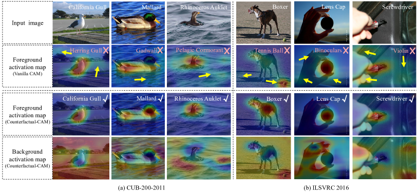
Figure 1: Given an input image, we visualize the foreground detected by the vanilla CAM and Counterfactual-CAM respectively, as well as the complementary background decoupled from Counterfactual-CAM. The pink labels and yellow arrows indicate the incorrect prediction category and the regions suffering from “biased activation”, respectively.

Weakly-supervised object localization (WSOL) focuses on localizing target objects in images using only image-level labels [8; 24; 15]. Previous approaches  [25; 7; 26; 37; 13; 36] have relied on class activation maps (CAMs) [48] to segment the highest activation area as a coarse object localization. However, these CAM-based methods, which learn with image-level labels, encounter difficulties in distinguishing between the object foreground and its co-occurring background, leading to the “biased activation” problem. Figure 1 illustrates how prior CAM-based methods incorrectly activate adjacent background regions, resulting in erroneous classification and localization.

To address the “biased activation” issue, some methods [43; 26] have employed the structural causal model (SCM) to explore the causality among the image, context, and image label. These studies have revealed the context (e.g., background) serves as a confounder, leading the detection model to learn spurious correlations between pixels and labels. Based on the investigation, CONTA [43] utilizes backdoor adjustment [21] and the do-operator $P(Y|do(X))$ to mitigate the confounding effect of context on image and pursue the pure causality between image and label. Similarly, CI-CAM [26] incorporates causal intervention into the WSOL model by using a causal context pool to address the entangled context problem. However, these approaches assume that all relevant confounding variables have been measured in the causal analysis since neglecting unmeasured confounders can result in biased prediction and incomplete mitigation of the confounding effects [11; 6; 45]. Nevertheless, integrally pinpointing all the confounders remains challenging in complex scenarios.

In contrast to the aforementioned approaches, we propose to solve the “biased activation” problem caused by the co-occurring background using counterfactual learning. A counterfactual refers to a hypothetical situation that deviates from the actual course of events [22]. By exploring counterfactuals, we can simulate scenarios in which the co-occurring background factors are altered untruly while the foreground is kept constant. Furthermore, training the model with these counterfactual scenarios using the correct labels can naturally lead the model to focus on the constant foreground content while disregarding the varying background information. Compared to the above methods based on causal intervention [43; 26], counterfactual learning avoids the necessity to pinpoint all relevant confounding variables and shows a more explicit ability to tackle the co-occurring context.

Following the counterfactual insight, we propose a novel Counterfactual Co-occurring Learning (CCL) paradigm, which synthesizes the counterfactual representations to eliminate the negative effect of the co-occurring background in the WSOL task. Specifically, we design a Counterfactual-CAM network by introducing a counterfactual representation perturbation mechanism to the vanilla CAM. This mechanism comprises two primary steps, i.e., co-occurring feature disentangling and counterfactual representation synthesis. Through a carefully designed co-occurring feature decoupler, the first step separates the co-occurring foreground and background features. To enforce both the independence between the co-occurring feature groups and the correct semantic interpretation of each group, we develop a new constraint loss to control the co-occurring feature disentangling process. The decoupled feature groups derived from the co-occurring feature disentangling step are utilized in the second step to generate counterfactual representations. These counterfactual representations are synthesized by the constant foreground and various backgrounds, which mitigate the co-occurring relationship between foreground and background. By training the detection model with these counterfactual representations, we compel the model to focus on the foreground content while disregarding the background information. Therefore, we can effectively address the “biased activation” problem. To sum up, the contributions of this paper are as follows.

• We propose a novel Counterfactual Co-occurring Learning (CCL) paradigm, in which we simulate counterfactual scenarios by pairing the constant foreground with unrealized backgrounds. To our best knowledge, it is the first attempt to utilize counterfactual learning to remove the negative effect of the co-occurring background in the WSOL task.

• We design a new network structure, dubbed Counterfactual-CAM, to embed the counterfactual representation perturbation mechanism into the vanilla CAM-based model. This mechanism achieves to decouple the foreground and co-occurring context as well as synthesizes the counterfactual representations.

• Extensive experiments conducted on multiple benchmark datasets demonstrate that Counterfactual-CAM successfully mitigates the “biased activation” problem and achieves remarkable improvements over prior state-of-the-art approaches.

2 Related Work

2.1 Weakly-supervised Object Localization

To address WSOL task, the most common solutions have relied on class activation maps (CAMs) [48] to segment the highest activation area as a coarse object localization. Prevailing works in this vein [12; 46; 1] try to solve the most discriminative region localization problem in vanilla CAM. To overcome the problem, the community has developed several methods [7; 9; 34; 12; 46; 1] that aim to perceive the entire object rather than the contracted and sparse discriminative regions. One category of methods [14; 35] addresses this issue by selecting positive proposals based on the discrepancy between their information and that of their surrounding contextual regions. WSLPDA [14] and TS²C [35] compare pixel values within a proposal and its neighboring contextual region. Another approach involves the use of a cascaded network structure [7; 9; 34] to expand and refine the initial prediction box. The output from the preceding stage acts as the pseudo ground-truth to supervise subsequent training stages. Furthermore, some methods, such as TP-WSL [12], ACoL [46], ADL [5], and MEIL [17] adopt an erasing strategy to compel the detector to identify subsequent discriminative regions. Additionally, SPOL [34] and ORNet [37] leverage the low-level feature to preserve more object detail information in the object localization phase.

Compared to the “most discriminative region localization” problem, the “biased activation” issue caused by the co-occurring background is less explored. This paper endeavors to tackle co-occurring backgrounds via counterfactual learning.

2.2 Causal Inference

Pearl et al. [22] proposed a three-step ladder of causation, consisting of association, intervention, and counterfactual analysis. Causal intervention as the effective solution in addressing confounder problem is widely used in various tasks, such as few-shot learning [40], long-tailed classification [29], and weakly-supervised segmentation [43] and localization [26]. Taking weakly-supervised segmentation and localization for example, without the instance- and pixel-label supervision, the context as a confounding factor leads image-level classification models to learn spurious correlations between pixels and labels. To solve this issue, CONTA [43] introduces the context adjustment based on backdoor adjustment [21] to remove the effect of context on the image. CI-CAM [26] uses a causal context pool to collect all contexts and then project them into the image feature maps for removing the influence of the specific context on the image feature maps. CONTA [43] and CI-CAM [26] rely on the belief that all relevant confounding variables have been measured and accounted for in the analysis. However, it can be challenging to identify all confounding variables in complex scenarios.

Counterfactual analysis can handle unmeasured or unknown confounding factors widely used in various tasks. For example, CMAT [4] proposes counterfactual critic multi-agent training in SGG. TDE [30] uses the counterfactual causality to infer the effect from bad bias and uses the total direct effect to achieve unbiased prediction. Chen et al. [3] generates counterfactual samples by masking critical objects in images or words in questions to reduce the language biases in VQA. CAL [23] leverages counterfactual analysis to fine-grained visual categorization and re-identification by maximizing the prediction of original and counterfactual attention. FairCL [44] generates counterfactual images for self-supervised contrastive learning to improve the fairness of learned representations.

In our work, we simulate counterfactual scenarios by pairing the constant foreground with various backgrounds. By training the model with these counterfactual scenarios using the correct label, we can naturally lead the model to focus on the constant foreground content while disregarding the varying background information. To our best knowledge, this work represents the first attempt to utilize counterfactual learning in this direction.

3 Methodology

Figure 2: (a) Building the structural causal model (SCM) in WSOL. (b) Cutting off the confounding effect of $B\rightarrow Y$ in WSOL. (c) Synthesizing counterfactual representations to remove the confounding effect of $B\rightarrow Y$. $O$: original image feature. $F$: foreground feature, $f_{1}\in F$. $B$: background feature, $b_{1},b_{2},b_{3}\in B$. $FB$: synthesized counterfactual representation. $Y$: image label, $y_{1}\in Y$.

3.1 Preliminaries

3.1.1 Combinational Class Activation Mapping

Given an image $I$, we obtain its class activation maps (CAMs) $M\in\mathbb{R}^{n\times h\times w}$ by using its feature maps $X\in\mathbb{R}^{c\times h\times w}$ and the weight matrix $W\in\mathbb{R}^{n\times c}$ of a classifier, where $n$, $c$, $h$, and $w$ indicate the number of classes, channel, height, and width respectively. Following the approach by Zhou et al. [48], the activation map $M_{i}$ of class $i$ among CAMs $M\in\mathbb{R}^{n\times h\times w}$ is given as follows.

$$M_{i}=\sum_{j}^{c}{W_{i,j}\cdot X_{j}},i\in\{1,2,\ldots,n\}.$$ (1)

However, NL-CCAM [39] argues the activation map $M_{k}$ of the prediction class $k$ often biases to over-small regions or sometimes even highlights background area. Thus, it proposes a combinational class activation mapping by combining all activation maps to generate a better localization map $H$.

$$H=\sum_{i}^{n}\gamma(i)\cdot M_{i},$$ (2)

where $\gamma(i)$ is a combinational weight associated with the rank index of class $i$. In this work, we build upon the localization approach proposed in NL-CCAM [39] but introduce significant improvements. Specifically, We equip the baseline with the ability to solve the “biased activation” problem.

3.1.2 Structural Causal Model

Inspired by CONTA [43], the structural causal model [21] is utilized to analyze the causality among original image feature $O$, foreground feature $F$, background feature $B$, and image label $Y$. The direct link shown in Figure 2 (a) denotes the causality between the two nodes: cause $\rightarrow$ effect [43].

$\bm{F\leftarrow O\rightarrow B}$: The two links indicate that the original image feature $O$ consists of foreground feature $F$ and background feature $B$. For example, in a fish picture, the foreground would be the “fish” and the background would be the “water”.

$\bm{F\rightarrow Y\leftarrow B}$: The two links indicate that the image prediction $Y$ of the original image is influenced by both the foreground feature $F$ and background feature $B$. However, without instance-level label supervision, the model inspection hard to distinguish between the foreground and its co-occurring background, resulting in the wrong activation. For example, 1) the background “water” region is wrongly activated as the “fish” foreground; 2) A “bird” drinking by the river is likely to be classified as a “fish” if the “water” is wrongly activated.

To remove the effect of $B\rightarrow Y$ in Figure 2 (b), we pair the foreground with all backgrounds, and then assign foreground category to these synthesized representations as shown in Figure 2 (c). Following the total probability formula in Equation 3, we obtain a pure prediction between the $F$ and $Y$.

$$P(Y|F) =\sum_{i}^{D}P(Y|F,b_{i})\cdot P(b_{i}|F),$$ (3)

where $D$ and $B=\{b_{1},b_{2},...,b_{D}\}$ are the number of training images and a comprehensive background set, respectively. If achieving the independence between foreground $F$ and background $B$, we can replace $P(b_{i}|F)$ with $P(b_{i})$. Since the occurrence probability of images in the dataset is roughly the same, we set $P(b_{i})$ to uniform $1/D$. Finally, $P(Y|F)$ can be replaced by $1/D\cdot\sum_{i}^{D}P(Y|F,b_{i})$.

3.2 Technical Details of Counterfactual-CAM

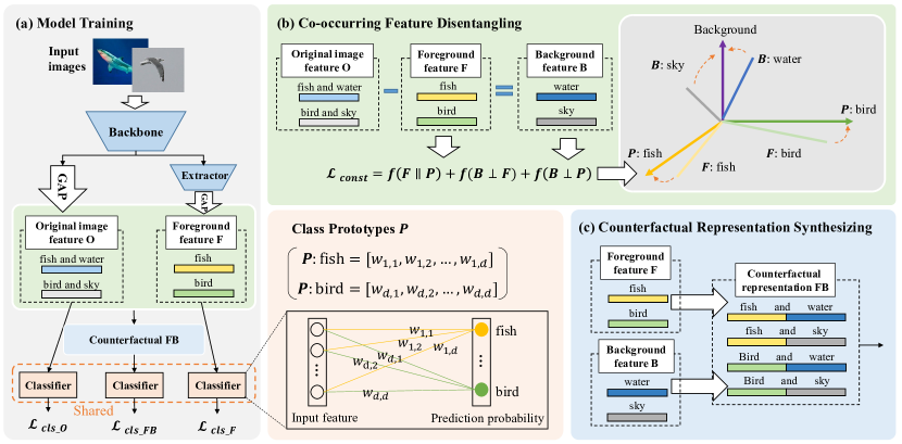
Figure 3: Overview of the proposed Counterfactual-CAM. (a) The learning process of Counterfactual-CAM. (b) Decoupling original image feature to foreground feature and background feature. $d$ denotes the length of the prototype feature. (c) Synthesizing counterfactual representations by coupling all foreground features and background features.

We implement a counterfactual model for the “biased activation” problem, dubbed Counterfactual-CAM. The core of it is the counterfactual representation perturbation mechanism, which consists of the co-occurring feature disentangling and counterfactual representation synthesis.

3.2.1 Co-occurring Feature Disentangling

Before presenting counterfactual representation synthesis, we first introduce the co-occurring feature decoupler. Given an image $I$, we first obtain its feature maps $X$ through a backbone. Then, $X$ is fed into a global average pooling (GAP) layer to produce the original feature $O\in\mathbb{R}^{d}$, where $d$ is the feature dimension. Meanwhile, $X$ is forwarded into a foreground extractor (i.e., two convolutional layers) and a GAP layer to generate image foreground feature $F\in\mathbb{R}^{d}$. Finally, we can separate background feature $B\in\mathbb{R}^{d}$ from original feature $O$ by subtracting foreground feature $F$ as shown in Figure 3 (b). To ensure the accuracy of the decoupling process, we set up the following two rules:

Rule 1. Foreground feature $F$ should be parallel with its corresponding class prototype $P$:

$$f(F\parallel P)=\sum_{i\neq k}^{n}L1Loss(\frac{F\times p_{i}}{|F|\times|p_{i}|},0)+L1Loss(\frac{F\times p_{k}}{|F|\times|p_{k}|},1),$$ (4)

where $n$ and $k$ indicate the number of classes and the category of foreground $F$, respectively. Inspired by T3A [10] and PCT [31], we use the weight in the classifier layer as class prototypes $P=\{p_{1},p_{2},...,p_{n}\}$. Equation 4 aims to align the $F$ with its corresponding class prototype $P$.

Rule 2. Background feature $B$ should be orthogonal from all $F$ and $P$:

$$f(B\perp F)=L1Loss(\frac{B\times F}{|B|\times|F|},0),f(B\perp P)=\sum_{i}^{n}L1Loss(\frac{B\times p_{i}}{|B|\times|p_{i}|},0),$$ (5)

where $L1Loss$ is the L1 norm function. $f(B\perp F)$ and $f(B\perp P)$ are optimal feature orthogonal strategy between background feature $B$ with all foreground features $F$ and class prototypes $P$.

Based on the above rules, we design a constraint loss $\mathcal{L}_{const}$ for thoroughly decoupling foreground feature $F$ and background feature $B$ from the original feature $O$, which is given as follows.

$$\mathcal{L}_{const}=f(F\parallel P)+f(B\perp F)+f(B\perp P).$$ (6)

Taking Figure 3 (b) for example, on one hand, $f(F\parallel P)$ aims to align foreground feature “$F:fish$” and class prototype “$P:fish$” (likewise for foreground feature “$F:bird$” and class prototype “$P:bird$”). On the other hand, $f(B\perp F)$ and $f(B\perp P)$ endeavor to keep orthogonal between background features “$B:water,sky$” with foreground features “$F:fish,bird$” and class prototypes “$P:fish,bird$”. Based on these, we can obtain the high-quality $F$ and $B$.

3.2.2 Counterfactual Representation Synthesizing

To remove the confounding effect of $B\rightarrow Y$ as shown in Figure 2 (b), we intend to leverage the total probability formula to pursue the pure causality between the cause $F$ and the effect $Y$ as shown in Equation 3. More concretely, we first collect all of the background features $B=\{b_{1},b_{2},b_{3},...\}$. Then, we pair each foreground feature $F$ with all background features $B=\{b_{1},b_{2},b_{3},...\}$ to synthesize a large number of counterfactual representations $FB$ as shown in Figure 2 (c). Finally, we assign a label to each counterfactual representation $FB$ according to its foreground category.

Taking Figure 3 (c) for example, we have the foreground features “fish” and “bird” as well as background features “water” and “sky”. After coupling foregrounds and backgrounds, we generate four synthesized representations: “fish and water”, “fish and sky”, “bird and water”, and “bird and sky”. Therein, “fish and sky” and ‘bird and water” are counterfactual representations. By aligning the prediction between the original image representations (i.e., “fish and water”) and counterfactual representations (i.e., “fish and sky”), we compel the CAM-based model to focus on the constant foreground “fish” while disregarding the “sky” and “water” information (likewise for “bird”).

3.2.3 Training Objective

Our proposed network not only learns to optimize the classification losses of the original image, foreground, and counterfactual representation but also learns to minimize the constraint loss $\mathcal{L}_{const}$ to ensure the accuracy of the co-occurring feature disentangling. Given an image, we first obtain the original image prediction score $s^{r}$, foreground prediction score $s^{f}$, and counterfactual representation prediction score $s^{fb}$. Then we train Counterfactual-CAM using the following loss function $\mathcal{L}^{train}$.

$$\mathcal{L}^{train}=CE(s^{r},y)+CE(s^{f},y)+CE(s^{fb},y)+\alpha\cdot\mathcal{L}_{const},$$ (7)

where $CE$, $y$, and $\alpha$ respectively denote the cross entropy function, image label, and hyperparameter.

3.3 Test-time Adaptation

The training and testing set usually suffer from a distribution gap on their co-occurring backgrounds, which further hinders CAM to highlight the accurate objects. To fully leverage the foreground hints present in test images to boost our CCL performance, we draw inspiration from the design of tent [33] and propose an online adaptation strategy with the following two considerations:

Consideration 1: The information from the test images provides valuable insights into the specific objects and their context present in the input images.

Consideration 2: Feeding the test-set foreground information into the detection model helps to activate the object foreground region and suppress the background activation region.

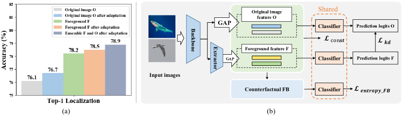
Figure 4: (a) Comparison of the prediction of the original image $O$, foreground $F$, and adaptation. (b) Overview of test-time adaptation, which finetunes the BN layers, foreground extractor, and classifier.

More concretely, for Consideration 1, we first aim to use the $\mathcal{L}_{const}$ (cf. Equation 6) to thoroughly decouple foreground and background from the original image. Then, minimizing the Shannon Entropy upon the prediction of the counterfactual representation to further align the constant foreground of the counterfactual representation and its corresponding class prototype. For Consideration 2, we take foreground knowledge to distill the original image prediction to force the model to pay more attention to foreground information. Finally, the total adaptation loss $\mathcal{L}^{adapt}$ is given as follows.

$$\mathcal{L}^{adapt}=\beta\cdot\mathcal{L}_{kd}+(1-\beta)\cdot(Entropy(Z^{fb})+\delta\cdot\mathcal{L}_{const}),$$ (8)

$$\mathcal{L}_{kd}=KL(\frac{\exp(Z^{r}/T)}{\sum_{j=1}^{n}\exp(Z^{r}_{j}/T)},\frac{\exp(Z^{f}/T)}{\sum_{j=1}^{n}\exp(Z^{f}_{j}/T)}),$$

where $KL$, $Z^{r}$, $Z^{f}$, and $Z^{fb}$ denote the Kullback-Leibler divergence loss function, original image logit, foreground logit, and counterfactual representation logit, respectively. $T$ and $n$ respectively denote the distillation temperature and the number of classes. $\beta$ and $\delta$ are the hyperparameters.

4 Experiments

4.1 Experimental Settings

Datasets. 1) CUB-200-2011 [32]. It focuses on the study of subordinate categorization, which contains $200$ bird species. Therein, it contains $5,994$ images with image-level labels in the training set and $5,794$ images with instance-level labels in the test set. 2) ILSVRC 2016 [24]. It consists of $1,000$ categories. Therein, it contains more than $1.2$ million images with image-level labels in the training set and $50,000$ images with instance-level labels in the validation set.

Evaluation Metrics. We use the Top-1 classification, Top-1 localization, and GT-known localization accuracy as the evaluation metrics. GT-known only considers localization regardless of classification result compared to Top-1 localization. It is worth noting that Top-1 Cls, Top-1 Loc, and GT-known respectively denote the Top-1 classification, Top-1 localization, and GT-known localization accuracy.

4.2 Comparisons with State-of-The-Art Methods

We compared Counterfactual-CAM with other state-of-the-art (SOTA) methods on the CUB-200-2011 [32] and ILSVRC 2016 [24] datasets as reported in Table 1 and Figure 5. The final experimental results of our method are the ensemble classification of the original image and foreground.

Table 1: Comparison with other state-of-the-art algorithms. The backbone is VGG16. The results of the first and second are shown in red and blue, respectively. $\ast$ indicates our re-implemented results.

Method	CUB-200-2011				ILSVRC 2016
	Top-1 Cls	Top-1 Loc	GT-known		Top-1 Cls	Top-1 Loc	GT-known
NL-CCAM [39]20	73.4	52.4	-		72.3	50.2	65.2
MEIL [17]20	74.8	57.5	73.8		70.3	46.8	-
PSOL [42]20	-	66.3	-		-	50.9	64.0
GCNet [16]20	76.8	63.2	-		-	-	-
RCAM [2]20	74.9	61.3	80.7		67.2	45.4	62.7
MCIR [1]21	72.6	58.1	-		71.2	51.6	66.3
SLT-Net [9]21	76.6	67.8	87.6		72.4	51.2	67.2
SPA [20]21	-	60.3	77.3		-	49.6	65.1
ORNet [37]21	77.0	67.7	-		71.6	52.1	-
FAM [18]21	77.3	69.3	89.3		70.9	52.0	71.7
PDM [19]22	76.9	67.3	82.2		68.7	51.1	69.3
BAS [36]22	-	71.3	91.1		-	53.0	69.6
BridgeGap [13]22	-	70.8	93.2		-	49.9	68.9
CREAM [38]22	-	70.4	91.0		-	52.4	68.3
Counterfactual-CAM	80.1	73.7	91.6		72.8	51.9	67.2

For the simple scenarios as on the CUB-200-2011 [32] whose background only consists of “water”, “sky”, “tree”, “grassland” etc. Counterfactual-CAM outperformed the current SOTA methods. Specifically, Counterfactual-CAM achieved $80.1\%$ Top-1 Cls and $73.7\%$ Top-1 Loc, surpassing FAM [18] in classification accuracy and BAS [36] in localization accuracy by $2.8\%$ and $2.4\%$, respectively. While Counterfactual-CAM lagged behind the GT-known SOTA method BridgeGap [13] by $1.6\%$ in GT-known accuracy, it still achieved a $2.9\%$ improvement over BridgeGap [13] in Top-1 Loc.

For more complex scenarios, such as ILSVRC 2016 [24] dataset, which exhibit diverse and intricate backgrounds, Counterfactual-CAM performed comparably to the current SOTA methods, particularly in Top-1 Cls. Notably, Counterfactual-CAM achieved a Top-1 Cls accuracy of $72.8\%$, surpassing the current SOTA SLT-Net [9] by $0.4\%$ and simultaneously improving Top-1 Loc by $0.7\%$. While Counterfactual-CAM showed a slight deficiency in localization performance compared to other SOTA methods, given the challenges posed by the large-scale ILSVRC 2016 dataset with its diverse scenarios and backgrounds, it still ranked among the top five in terms of localization performance.

To evaluate the robustness of Counterfactual-CAM, we conducted a complementary experiment by replacing VGG16 [27] with InceptionV3 [28] on the CUB-200-2011 dataset, as shown in Table 2. Counterfactual-CAM achieved the best performance across all evaluation metrics and outperformed other SOTA methods by a significant margin. Specifically, Counterfactual-CAM surpassed BAS [36], the best localization SOTA, by $5.0\%$ in Top-1 Loc and by $2.8\%$ in GT-known accuracy. Additionally, Counterfactual-CAM demonstrated exceptional performance in Top-1 Cls, exhibiting a $0.9\%$ improvement over the best classification SOTA FAM [18].

Overall, our experimental results highlight the effectiveness and robustness of Counterfactual-CAM across different datasets and backbones, establishing its superiority over existing SOTA methods.

Table 2: Comparison with other state-of-the-art algorithms on the CUB-200-2011 dataset. The backbone is InceptionV3. The results of the first and second are shown in red and blue, respectively.

Method	Top-1 Cls	Top-1 Loc	GT-known
PSOL [42]20	-	65.5	-
I2C [47]20	-	55.0	72.6
SLT-Net [9]21	76.4	66.1	86.5
SPA [20]21	-	53.5	72.1
FAM [18]21	81.3	70.7	87.3
PDM [19]22	-	64.3	79.6
BAS [36]22	-	73.3	92.2
CREAM [38]22	-	71.8	90.4
Counterfactual-CAM	82.2	78.3	95.0

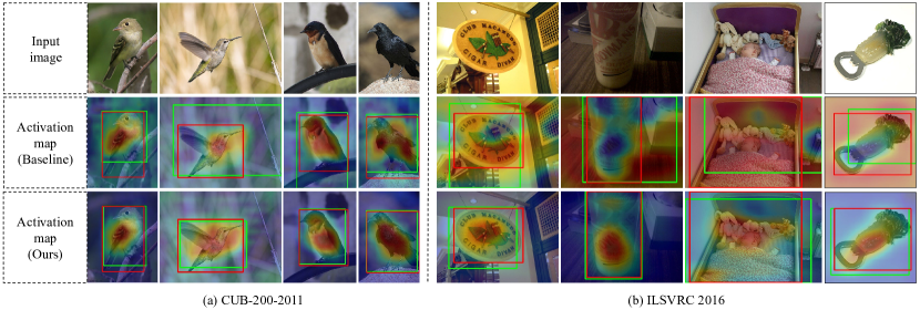
Figure 5: Qualitative object localization results compared with the baseline method. The predicted bounding boxes are in green, and the ground-truth boxes are in red.

4.3 Ablation Study

To demonstrate the effectiveness of counterfactual representation and constraint loss, we conducted several ablation studies on the CUB-200-2011 [32] and ILSVRC 2016 [24] datasets as presented in Table 3.

Counterfactual Representation. We observed training the baseline model with counterfactual representation led to significant improvements across all evaluation metrics. Specifically, when using VGG16 [27] as the backbone, counterfactual representation resulted in an additional $3.1\%$, $4.4\%$, and $1.9\%$ improvement in Top-1 Cls, Top-1 Loc, and GT-known accuracy, respectively, on the CUB-200-2011 dataset. Similarly, counterfactual representation demonstrated outstanding performance on the ILSVRC 2016 dataset, improving Top-1 Loc and GT-known accuracy by $2.5\%$ and $2.9\%$, respectively, compared to the baseline. Remarkably, counterfactual representation also exhibited remarkable performance when combined with InceptionV3 [28] as the backbone. For instance, they achieved an additional $3.1\%$ improvement in Top-1 Cls and a $2.0\%$ improvement in Top-1 Loc compared to the baseline.

Constraint Loss. On the CUB-200-2011 dataset, employing the constraint loss resulted in respective improvements of $1.0\%$ and $0.3\%$ in Top-1 Cls and Top-1 Loc when using VGG16 as the backbone. When the backbone was InceptionV3, training the model with the constraint loss led to additional improvements of $1.1\%$ and $1.2\%$ in Top-1 Loc and GT-known accuracy, respectively. In more complex scenarios, such as the ILSVRC 2016 dataset, the constraint loss remained crucial, resulting in additional improvements of $0.3\%$ in both Top-1 Loc and GT-known accuracy.

These ablation studies confirm the effectiveness of counterfactual representation and the constraint loss on both the CUB-200-2011 and ILSVRC 2016 datasets.

Table 3: Ablation studies on the CUB-200-2011 and ILSVRC 2016 datasets. 1) Baseline: NL-CCAM [39], 2) Counterfactual: counterfactual representation. 3) Constraint: constraint loss.

Dataset	Backbone	Baseline	Counterfactual	Constraint	Top-1 Cls	Top-1 Loc	GT-known
CUB-200-2011 test set	VGG16	$\surd$			76.0	69.0	90.5
		$\surd$	$\surd$		79.1	73.4	92.4
		$\surd$	$\surd$	$\surd$	80.1	73.7	91.6
	IncepV3	$\surd$			79.1	75.2	94.6
		$\surd$	$\surd$		82.2	77.2	93.8
		$\surd$	$\surd$	$\surd$	82.2	78.3	95.0
ILSVRC 2016 val set	VGG16	$\surd$			72.4	49.1	64.0
		$\surd$	$\surd$		72.8	51.6	66.9
		$\surd$	$\surd$	$\surd$	72.8	51.9	67.2

4.4 Test-time Adaptation Experiment

Table 4: Comparison with different adaptation on CUB-200-2011.

Method	VGG16		InceptionV3
	Top-1 Loc	GT-known	Top-1 Loc	GT-known
Without adaptation	73.7	91.6	78.3	95.0
Adaptation with tent [33]	74.0	93.1	78.7	95.8
Adaptation with ours	74.7	93.2	78.9	96.0

To highlight the importance of test-time adaptation, we conducted experiments on the CUB-200-2011 dataset [32]. In Table 4, we observed significant improvements in localization performance with both types of adaptation approaches. Furthermore, our adaptation approach outperformed tent [33] comprehensively. Specifically, when using VGG16 [27] as the backbone, our adaptation approach achieved an additional $1.0\%$ and $1.6\%$ improvement in Top-1 Loc and GT-known accuracy, respectively, outperforming tent by $0.7\%$ and $0.1\%$. Similarly, when using InceptionV3 [28] as the backbone, our adaptation approach yielded an additional $0.6\%$ and $1.0\%$ improvement in Top-1 Loc and GT-known accuracy, respectively, outperforming tent by $0.2\%$ in both metrics. These results underscore the superior performance of our adaptation approach compared to the tent in terms of improving localization accuracy when applied during test-time in Counterfactual-CAM.

5 Conclusion

In this paper, we make an early attempt to tackle the “biased activation” problem caused by co-occurring background via Counterfactual Co-occurring Learning (CCL) paradigm. Specifically, we design the counterfactual representation perturbation mechanism, which consists of co-occurring feature disentangling and counterfactual representation synthesis. The former is responsible for decoupling the foreground and its co-occurring background from the original image. The latter synthesizes counterfactual representation pairing the constant foreground with various backgrounds. By aligning the prediction between the original image representations and counterfactual representations, we compel the detection model to focus on the constant foreground information while disregarding the different background information. Therefore, we can eliminate the effect of the co-occurring background, thereby addressing the “biased localization” problem.

Appendix

A Implementation Details

We adopted the VGG16 [27] and InceptionV3 [28] pre-trained on the ImageNet [24] as our backbones. The extractor proposed in our network comprises two convolutional layers and two activation functions. Notably, we employed RandAugment [28] for data augmentation on the CUB-200-2011 [32] dataset during training.

For the VGG16 [27] backbone, we fine-tuned our network by resizing input images to $344\times 344$ and randomly cropping it to $224\times 224$. Besides, we used a learning rate of $0.0005$, a batch size of 12, 100 epochs, $\alpha=0.001$, $\beta=0.2$, $\delta=0.012$, and a temperature of $T=15$ on the CUB-200-2011 [32] dataset. During testing, we performed a central crop of $224\times 224$, following the approach in [36, 34, 42, 5, 41]. Similarly, on the ILSVRC 2016 [24] dataset, we first resized input images to $288\times 288$ and randomly cropped it to $224\times 224$. Besides, we used a learning rate of $0.0000585$, a batch size of 36, and 20 epochs, with $\alpha=0.12$. During testing on this dataset, we centrally cropped them to $224\times 224$ [36, 34, 42, 5, 41]. Finally, we set the segmentation threshold to $0.14$ and $0.16$ for generating bounding boxes on the CUB-200-2011 and ILSVRC 2016 datasets, respectively.

For the InceptionV3 [28] backbone, we fine-tuned our network by resizing input images to $500\times 500$ and randomly cropping it to $299\times 299$. Besides, we used a learning rate of $0.0001$, a batch size of 12, 100 epochs, $\alpha=0.0001$, $\beta=0.1$, $\delta=0.012$, and a temperature of $T=30$ on the CUB-200-2011 [32] dataset. During testing, we performed a central crop of $299\times 299$ [36, 34, 42, 5, 41], followed by setting the segmentation threshold to $0.21$ for generating bounding boxes.

B Broader Impacts

This work represents the first attempt to address the influence of co-occurring backgrounds in the weakly-supervised object localization (WSOL) task through the Counterfactual Co-occurring Learning (CCL) paradigm. Traditional weakly supervised learning approaches require extensive manual effort and resources to search for and label images across diverse scenes to mitigate the impact of co-occurring backgrounds. Furthermore, objects seldom exist in isolation, as they often co-occur the specific contexts [43], so sometimes it might be hard to break the co-occurrence relationships between foregrounds and backgrounds in real-world pictures. But, our proposed CCL paradigm enables us to effortlessly disrupt the co-occurrence relationship between foreground and background by synthesizing a large number of counterfactual representations. Consequently, we can effectively eliminate the influence of co-occurring backgrounds without human involvement.

Overall, the impact of our proposed CCL paradigm on the research community is undeniably positive.

C Limitations

Despite being a pioneering attempt to decouple foreground and co-occurring backgrounds in original images in the WSOL task, our proposed counterfactual representation perturbation mechanism still has one limitation. Specifically, this mechanism heavily relies on the availability of foreground and background information during the training phase. If the co-occurring background in the test set differs significantly from the training set or contains unique characteristics, it may struggle to effectively eliminate the influence of co-occurring backgrounds, leading to reduced performance and accuracy on unseen data. To address this issue, we have implemented a test-time adaptation to specifically decouple and collect the foreground and background information in the test set. However, in addition to the foreground and background information in the test set, there may be other valuable information that we have not effectively utilized in our test-time adaptation.

References

- [1] Sadbhavana Babar and Sukhendu Das. Where to look?: Mining complementary image regions for weakly supervised object localization. In Proceedings of the IEEE/CVF Winter Conference on Applications of Computer Vision, 2021.
- [2] Wonho Bae, Junhyug Noh, and Gunhee Kim. Rethinking class activation mapping for weakly supervised object localization. In European Conference on Computer Vision, 2020.
- [3] Long Chen, Xin Yan, Jun Xiao, Hanwang Zhang, Shiliang Pu, and Yueting Zhuang. Counterfactual samples synthesizing for robust visual question answering. In Proceedings of the IEEE/CVF conference on computer vision and pattern recognition, 2020.
- [4] Long Chen, Hanwang Zhang, Jun Xiao, Xiangnan He, Shiliang Pu, and Shih-Fu Chang. Counterfactual critic multi-agent training for scene graph generation. In Proceedings of the IEEE/CVF International Conference on Computer Vision, 2019.
- [5] Junsuk Choe and Hyunjung Shim. Attention-based dropout layer for weakly supervised object localization. In Proceedings of the IEEE Conference on Computer Vision and Pattern Recognition, 2019.
- [6] Iván Díaz and Mark J van der Laan. Sensitivity analysis for causal inference under unmeasured confounding and measurement error problems. The international journal of biostatistics, 2013.
- [7] Ali Diba, Vivek Sharma, Ali Pazandeh, Hamed Pirsiavash, and Luc Van Gool. Weakly supervised cascaded convolutional networks. In Proceedings of the IEEE conference on computer vision and pattern recognition, 2017.
- [8] Mark Everingham, Luc Van Gool, Christopher KI Williams, John Winn, and Andrew Zisserman. The pascal visual object classes (voc) challenge. IJCV, 2010.
- [9] Guangyu Guo, Junwei Han, Fang Wan, and Dingwen Zhang. Strengthen learning tolerance for weakly supervised object localization. In Proceedings of the IEEE/CVF Conference on Computer Vision and Pattern Recognition, 2021.
- [10] Yusuke Iwasawa and Yutaka Matsuo. Test-time classifier adjustment module for model-agnostic domain generalization. Advances in Neural Information Processing Systems, 2021.
- [11] Nathan Kallus, Xiaojie Mao, and Masatoshi Uehara. Causal inference under unmeasured confounding with negative controls: A minimax learning approach. arXiv preprint arXiv:2103.14029, 2021.
- [12] Dahun Kim, Donghyeon Cho, Donggeun Yoo, and In So Kweon. Two-phase learning for weakly supervised object localization. In Proceedings of the IEEE International Conference on Computer Vision, 2017.
- [13] Eunji Kim, Siwon Kim, Jungbeom Lee, Hyunwoo Kim, and Sungroh Yoon. Bridging the gap between classification and localization for weakly supervised object localization. In Proceedings of the IEEE/CVF Conference on Computer Vision and Pattern Recognition, 2022.
- [14] Dong Li, Jia-Bin Huang, Yali Li, Shengjin Wang, and Ming-Hsuan Yang. Weakly supervised object localization with progressive domain adaptation. In Proceedings of the IEEE/CVF Conference on Computer Vision and Pattern Recognition, 2016.
- [15] Tsung-Yi Lin, Michael Maire, Serge Belongie, James Hays, Pietro Perona, Deva Ramanan, Piotr Dollár, and C Lawrence Zitnick. Microsoft coco: Common objects in context. In ECCV, 2014.
- [16] Weizeng Lu, Xi Jia, Weicheng Xie, Linlin Shen, Yicong Zhou, and Jinming Duan. Geometry constrained weakly supervised object localization. In European Conference on Computer Vision, 2020.
- [17] Jinjie Mai, Meng Yang, and Wenfeng Luo. Erasing integrated learning: A simple yet effective approach for weakly supervised object localization. In CVPR, 2020.
- [18] Meng Meng, Tianzhu Zhang, Qi Tian, Yongdong Zhang, and Feng Wu. Foreground activation maps for weakly supervised object localization. In Proceedings of the IEEE/CVF International Conference on Computer Vision, 2021.
- [19] Meng Meng, Tianzhu Zhang, Wenfei Yang, Jian Zhao, Yongdong Zhang, and Feng Wu. Diverse complementary part mining for weakly supervised object localization. IEEE Transactions on Image Processing, 2022.
- [20] Xingjia Pan, Yingguo Gao, Zhiwen Lin, Fan Tang, Weiming Dong, Haolei Yuan, Feiyue Huang, and Changsheng Xu. Unveiling the potential of structure preserving for weakly supervised object localization. In Proceedings of the IEEE/CVF Conference on Computer Vision and Pattern Recognition, 2021.
- [21] Judea Pearl, Madelyn Glymour, and Nicholas P Jewell. Causal inference in statistics: A primer. 2016.
- [22] Judea Pearl and Dana Mackenzie. The book of why: the new science of cause and effect. 2018.
- [23] Yongming Rao, Guangyi Chen, Jiwen Lu, and Jie Zhou. Counterfactual attention learning for fine-grained visual categorization and re-identification. In Proceedings of the IEEE/CVF International Conference on Computer Vision, 2021.
- [24] Olga Russakovsky, Jia Deng, Hao Su, Jonathan Krause, Sanjeev Satheesh, Sean Ma, Zhiheng Huang, Andrej Karpathy, Aditya Khosla, Michael Bernstein, et al. Imagenet large scale visual recognition challenge. IJCV, 2015.
- [25] Ramprasaath R Selvaraju, Michael Cogswell, Abhishek Das, Ramakrishna Vedantam, Devi Parikh, and Dhruv Batra. Grad-cam: Visual explanations from deep networks via gradient-based localization. In ICCV, 2017.
- [26] Feifei Shao, Yawei Luo, Li Zhang, Lu Ye, Siliang Tang, Yi Yang, and Jun Xiao. Improving weakly supervised object localization via causal intervention. In Proceedings of the 29th ACM International Conference on Multimedia, 2021.
- [27] Karen Simonyan and Andrew Zisserman. Very deep convolutional networks for large-scale image recognition. In arXiv, 2014.
- [28] Christian Szegedy, Vincent Vanhoucke, Sergey Ioffe, Jon Shlens, and Zbigniew Wojna. Rethinking the inception architecture for computer vision. In Proceedings of the IEEE conference on computer vision and pattern recognition, 2016.
- [29] Kaihua Tang, Jianqiang Huang, and Hanwang Zhang. Long-tailed classification by keeping the good and removing the bad momentum causal effect. arXiv preprint arXiv:2009.12991, 2020.
- [30] Kaihua Tang, Yulei Niu, Jianqiang Huang, Jiaxin Shi, and Hanwang Zhang. Unbiased scene graph generation from biased training. In Proceedings of the IEEE/CVF Conference on Computer Vision and Pattern Recognition, 2020.
- [31] Korawat Tanwisuth, Xinjie Fan, Huangjie Zheng, Shujian Zhang, Hao Zhang, Bo Chen, and Mingyuan Zhou. A prototype-oriented framework for unsupervised domain adaptation. Advances in Neural Information Processing Systems, 2021.
- [32] Catherine Wah, Steve Branson, Peter Welinder, Pietro Perona, and Serge Belongie. The caltech-ucsd birds-200-2011 dataset. 2011.
- [33] Dequan Wang, Evan Shelhamer, Shaoteng Liu, Bruno Olshausen, and Trevor Darrell. Tent: Fully test-time adaptation by entropy minimization. arXiv preprint arXiv:2006.10726, 2020.
- [34] Jun Wei, Qin Wang, Zhen Li, Sheng Wang, S Kevin Zhou, and Shuguang Cui. Shallow feature matters for weakly supervised object localization. In Proceedings of the IEEE/CVF Conference on Computer Vision and Pattern Recognition, 2021.
- [35] Yunchao Wei, Zhiqiang Shen, Bowen Cheng, Honghui Shi, Jinjun Xiong, Jiashi Feng, and Thomas Huang. Ts2c: Tight box mining with surrounding segmentation context for weakly supervised object detection. In Proceedings of the European Conference on Computer Vision (ECCV), 2018.
- [36] Pingyu Wu, Wei Zhai, and Yang Cao. Background activation suppression for weakly supervised object localization. In 2022 IEEE/CVF Conference on Computer Vision and Pattern Recognition (CVPR), 2022.
- [37] Jinheng Xie, Cheng Luo, Xiangping Zhu, Ziqi Jin, Weizeng Lu, and Linlin Shen. Online refinement of low-level feature based activation map for weakly supervised object localization. In Proceedings of the IEEE/CVF International Conference on Computer Vision, 2021.
- [38] Jilan Xu, Junlin Hou, Yuejie Zhang, Rui Feng, Rui-Wei Zhao, Tao Zhang, Xuequan Lu, and Shang Gao. Cream: Weakly supervised object localization via class re-activation mapping. In Proceedings of the IEEE/CVF Conference on Computer Vision and Pattern Recognition, 2022.
- [39] Seunghan Yang, Yoonhyung Kim, Youngeun Kim, and Changick Kim. Combinational class activation maps for weakly supervised object localization. In WACV, 2020.
- [40] Zhongqi Yue, Hanwang Zhang, Qianru Sun, and Xian-Sheng Hua. Interventional few-shot learning. arXiv preprint arXiv:2009.13000, 2020.
- [41] Sangdoo Yun, Dongyoon Han, Seong Joon Oh, Sanghyuk Chun, Junsuk Choe, and Youngjoon Yoo. Cutmix: Regularization strategy to train strong classifiers with localizable features. In Proceedings of the IEEE/CVF international conference on computer vision, 2019.
- [42] Chen-Lin Zhang, Yun-Hao Cao, and Jianxin Wu. Rethinking the route towards weakly supervised object localization. In Proceedings of the IEEE/CVF Conference on Computer Vision and Pattern Recognition, 2020.
- [43] Dong Zhang, Hanwang Zhang, Jinhui Tang, Xiansheng Hua, and Qianru Sun. Causal intervention for weakly-supervised semantic segmentation. arXiv preprint arXiv:2009.12547, 2020.
- [44] Fengda Zhang, Kun Kuang, Long Chen, Yuxuan Liu, Chao Wu, and Jun Xiao. Fairness-aware contrastive learning with partially annotated sensitive attributes. In The Eleventh International Conference on Learning Representations, 2023.
- [45] Xiang Zhang, Douglas E Faries, Hu Li, James D Stamey, and Guido W Imbens. Addressing unmeasured confounding in comparative observational research. Pharmacoepidemiology and drug safety, 2018.
- [46] Xiaolin Zhang, Yunchao Wei, Jiashi Feng, Yi Yang, and Thomas S Huang. Adversarial complementary learning for weakly supervised object localization. In Proceedings of the IEEE Conference on Computer Vision and Pattern Recognition, 2018.
- [47] Xiaolin Zhang, Yunchao Wei, and Yi Yang. Inter-image communication for weakly supervised localization. In European Conference on Computer Vision, 2020.
- [48] Bolei Zhou, Aditya Khosla, Agata Lapedriza, Aude Oliva, and Antonio Torralba. Learning deep features for discriminative localization. In CVPR, 2016.