Revisit and Outstrip Entity Alignment:
A Perspective of Generative Models

Abstract

Recent embedding-based methods have achieved great successes on exploiting entity alignment from knowledge graph (KG) embeddings of multiple modals. In this paper, we study embedding-based entity alignment (EEA) from a perspective of generative models. We show that EEA is a special problem where the main objective is analogous to that in a typical generative model, based on which we theoretically prove the effectiveness of the recently developed generative adversarial network (GAN)-based EEA methods. We then reveal that their incomplete objective limits the capacity on both entity alignment and entity synthesis (i.e., generating new entities). We mitigate this problem by introducing a generative EEA (abbr., GEEA) framework with the proposed mutual variational autoencoder (M-VAE) as the generative model. M-VAE can convert an entity from one KG to another and generate new entities from random noise vectors. We demonstrate the power of GEEA with theoretical analysis and empirical experiments on both entity alignment and entity synthesis tasks.

1 Introduction

As one of the most prevalent tasks in the knowledge graph (KG) area, entity alignment (EA) has recently made great progress and developments with the support of the embedding techniques [1, 2, 3, 4, 5, 6, 7, 8, 9, 10, 11, 12, 13, 14, 15, 16, 17, 18, 19]. By encoding the relational and other information into low-dimension vectors, the embedding-based entity alignment (EEA) methods are friendly to development and deployment, and simultaneously achieve state-of-the-art performance on many benchmarks.

The objective of EA is to maximize the conditional probability $p(y|x)$, where $x$, $y$ are a pair of aligned entities belonging to source KG ${\mathcal{X}}$ and target KG ${\mathcal{Y}}$, respectively. If we view $x$ as the input and $y$ the label (and vice versa), the problem can be solved by a discriminative model. To this end, we need an EEA model which comprises an encoder module and a fusion layer [12, 13, 14, 15, 16, 17] (see Figure 1). The encoder module uses different encoders to encode the multi-modal information to same low-dimensional embeddings (sub-embeddings). Then, the fusion layer combines these sub-embeddings to one joint embedding as output.

We also need a predictor, as shown in the yellow area in Figure 1. The predictor is usually independent to the EEA model and parameterized with neural layers [1, 7] or based on the embedding distance [2, 3]. In either case, it learns the probability $p(y|x)$ where $p(y|x)=1$ if the two entities $x$, $y$ are aligned and $0$ otherwise. The difference mainly rests on data augmentation. The existing methods leverage different strategies to construct more training data, e.g., negative sampling [2, 4, 6, 7, 8, 11, 12, 13, 14, 15, 16, 17] and bootstrapping [3, 8, 9]. In this paper, we show that if we study EEA from a generative perspective, we can interpret the negative sampling algorithms and the generative adversarial network (GAN)-based methods [9, 10, 11] theoretically and tighten the objective of EEA a further step.

In fact, entity alignment is not the ultimate aim of many applications. People use the results of entity alignment to enrich each other KG, but many entities in the source KG may not have aligned entities in the target KG (i.e., the dangling entities) [20, 21, 22]. If we can convert these entities from the source KG to the target KG, a major expenditure of time and effort will be saved. Also, generating new entities from random variables may contribute to the fields like Metaverse and video games where the design of virtual characters still rely on hand-crafted features and random algorithms [23, 24]. Therefore, we propose a new task called entity synthesis to generating new entities conditionally/unconditionally.

We propose a generative EEA (abbr., GEEA) framework with the mutual variational autoencoder (M-VAE) to mutually encode/decode entities between source and target KGs. Unlike the existing GAN-based methods [9, 10, 11], our GEEA is capable of generating concrete features (e.g., the exact neighborhood or attribute information of a new entity) rather than only the inexplicable embeddings. We also propose the prior reconstruction and post reconstruction to control the generation process. Briefly, the prior reconstruction is used to generate specific features for each modal, while the post reconstruction ensures these different kinds of features belong to one entity.

We summarize our contributions as follows: (1) We show that current EEA methods can be understood and explained from a generative perspective. (2) We propose GEEA for both entity alignment and entity synthesis, and prove its effectiveness in theory. (3) We conduct experiments to verify the performance of GEEA, where it achieves the state-of-the-art performance in entity alignment and generates high-quality new entities in entity synthesis.

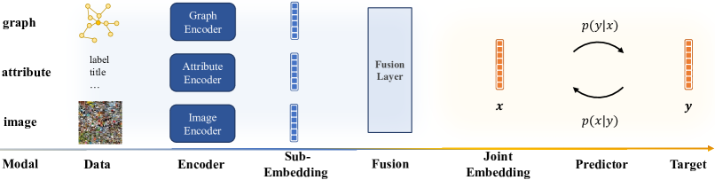
Figure 1: Illustration of embedding-based entity alignment. The modules in the blue area belong to the EEA model, while those in the yellow area belong to the predictor.

2 Revisit Embedding-based Entity Alignment

In this section, we revisit embedding-based entity alignment by a theoretical analysis of how the generative models contribute to entity alignment learning, and then discuss their limitations.

2.1 Embedding-based Entity Alignment

Entity alignment aims to find the implicitly aligned entity pairs $\{(x,y)|x\in{\mathcal{X}},y\in{\mathcal{Y}}\}$, where ${\mathcal{X}}$, ${\mathcal{Y}}$ denote the source and target entity sets, and $(x,y)$ is a pair of aligned entities that refer to the same object in real world. An EEA model ${\mathcal{M}}$ takes a small number of aligned entity pairs ${\mathcal{S}}$ (a.k.a., seed alignment set) as training data to infer the remaining alignment pairs ${\mathcal{T}}$ in the testing set. The relational graph information ${\mathcal{G}}_{x}$, ${\mathcal{G}}_{y}$, the attribute information ${\mathcal{A}}_{x}$, ${\mathcal{A}}_{y}$, and the other types of information (e.g., image information ${\mathcal{I}}_{x}$, ${\mathcal{I}}_{y}$) are given as features to ${\mathcal{X}}$, ${\mathcal{Y}}$.

Specifically, the model ${\mathcal{M}}$ takes the discrete features $x=(g_{x},a_{x},i_{x},...)$ of an entity $x$ as input, where $g_{x}$, $a_{x}$, $i_{x}$ denote the relational graph information, attribute information and image information of $x$, respectively. The output comprises the latent embeddings for each modal and a joint embedding ${\mathbf{x}}$ which is a combination of all modals:

$${\mathbf{x}}={\mathcal{M}}(x) =\textit{Linear}(\textit{Concat}({\mathcal{M}}_{g}(g_{x}),{\mathcal{M}}_{a}(a_{x}),{\mathcal{M}}_{i}(i_{x}),...))$$ (1)

$$=\textit{Linear}(\textit{Concat}({\mathbf{g}}_{x},{\mathbf{a}}_{x},\mathbf{i}_{x},...)),$$ (2)

where ${\mathcal{M}}_{g}$, ${\mathcal{M}}_{a}$, and ${\mathcal{M}}_{i}$ denote the EEA encoders for different modals (see Figure 1), and ${\mathbf{g}}_{x}$, ${\mathbf{a}}_{x}$, $\mathbf{i}_{x}$ denote the embeddings of different modals. Similarly, we can obtain ${\mathbf{y}}$ by ${\mathbf{y}}={\mathcal{M}}(y)$.

2.2 EEA Benefits from the Generative Objectives

Let $x\sim{\mathcal{X}}$, $y\sim{\mathcal{Y}}$ be two entities sampled from the entity sets ${\mathcal{X}}$, ${\mathcal{Y}}$, respectively. The main target of EEA is to learn a predictor to predict the conditional probability $p_{\theta}({\mathbf{x}}|{\mathbf{y}})$ (and reversely $p_{\theta}({\mathbf{y}}|{\mathbf{x}})$), where $\theta$ is the parameter set. For simplicity, we assume that the reverse function $p_{\theta}({\mathbf{y}}|{\mathbf{x}})$ shares this parameter set with $p_{\theta}({\mathbf{x}}|{\mathbf{y}})$.

Now, suppose that one wants to learn a generative model to generate entity embeddings:

$$\log p({\mathbf{x}}) =\log p({\mathbf{x}})\int p_{\theta}({\mathbf{y}}|{\mathbf{x}})d{\mathbf{y}}$$ (3)

$$=\mathbb{E}_{p_{\theta}({\mathbf{y}}|{\mathbf{x}})}\Big{[}\log\frac{p({\mathbf{x}},{\mathbf{y}})}{p_{\theta}({\mathbf{y}}|{\mathbf{x}})}\Big{]}+D_{\mathrm{KL}}(p_{\theta}({\mathbf{y}}|{\mathbf{x}})\parallel p({\mathbf{y}}|{\mathbf{x}})),$$ (4)

where the left hand of Equation (4) is usually called ELBO [25], and the right hand is the KL divergence [26] between our parameterized distribution $p_{\theta}({\mathbf{y}}|{\mathbf{x}})$ (i.e.,the predictor) and the true distribution $p({\mathbf{y}}|{\mathbf{x}})$. The complete derivation can be found in Appendix A.

In typical generative learning, $p({\mathbf{y}}|{\mathbf{x}})$ is intractable as ${\mathbf{y}}$ is a noise variable sampled from normal distribution and thus $p({\mathbf{y}}|{\mathbf{x}})$ is unknown. However, in EEA, we can obtain a few samples by the use of training set, which yields a classical negative sampling loss [2, 3, 4, 6, 7, 8, 11, 12, 13, 14, 15, 16, 17]:

$$\mathcal{L}_{\text{ns}}=\sum_{i}[-\log(p_{\theta}({\mathbf{y}}^{i}|{\mathbf{x}}^{i})p({\mathbf{y}}^{i}|{\mathbf{x}}^{i}))+\frac{1}{N_{\text{ns}}}\sum_{j\neq i}\log\big{(}p_{\theta}({\mathbf{y}}^{j}|{\mathbf{x}}^{i})(1-p({\mathbf{y}}^{j}|{\mathbf{x}}^{i}))\big{)}],$$ (5)

where $({\mathbf{y}}^{i},{\mathbf{x}}^{i})$ denotes a pair of aligned entities in the training data, and the randomly sampled entity ${\mathbf{y}}^{j}$ is regarded as the negative entity. $i$, $j$ are the entity IDs. $N_{\text{ns}}$ is the normalization constant. Here, $\mathcal{L}_{\text{ns}}$ is written in a form of cross-entropy loss with the label $p({\mathbf{y}}^{j}|{\mathbf{x}}^{i})$ as follows:

$$p({\mathbf{y}}^{j}|{\mathbf{x}}^{i})=\begin{cases}0,\quad&i\neq j,\\ 1,\quad&i=j\end{cases}$$ (6)

Considering that there are only a small number of aligned entity pairs as training data in EEA, the observation of $p({\mathbf{y}}|{\mathbf{x}})$ may be biased and limited. To alleviate this problem, the recent GAN-based methods [9, 10, 11] propose to leverage the entities out of training set for unsupervised learning. Their common idea is to make the entity embeddings from different KGs indiscriminative to a discriminator, and the underlying aligned entities shall be encoded in the same way and have similar embeddings. To formally prove this idea, we dissect the ELBO in Equation (4) as follows:

$$\mathbb{E}_{p_{\theta}({\mathbf{y}}|{\mathbf{x}})}\Big{[}\log\frac{p({\mathbf{x}},{\mathbf{y}})}{p_{\theta}({\mathbf{y}}|{\mathbf{x}})}\Big{]} =\mathbb{E}_{p_{\theta}({\mathbf{y}}|{\mathbf{x}})}\Big{[}\log p_{\theta}({\mathbf{x}}|{\mathbf{y}})\Big{]}-D_{\mathrm{KL}}(p_{\theta}({\mathbf{y}}|{\mathbf{x}})\parallel p({\mathbf{y}}))$$ (7)

The complete derivation can be found in Appendix A. Therefore, we have:

$$\log p({\mathbf{x}})=\underbrace{\vphantom{\mathbb{E}_{p_{\theta}({\mathbf{y}}|{\mathbf{x}})}\Big{[}\log p_{\theta}({\mathbf{x}}|{\mathbf{y}})\Big{]}}\mathbb{E}_{p_{\theta}({\mathbf{y}}|{\mathbf{x}})}\Big{[}\log p_{\theta}({\mathbf{x}}|{\mathbf{y}})\Big{]}}_{\text{reconstruction term}}-\underbrace{\vphantom{\mathbb{E}_{p_{\theta}({\mathbf{y}}|{\mathbf{x}})}\Big{[}\log p_{\theta}({\mathbf{x}}|{\mathbf{y}})\Big{]}}D_{\mathrm{KL}}(p_{\theta}({\mathbf{y}}|{\mathbf{x}})\parallel p({\mathbf{y}}))}_{\text{distribution matching term}}+\underbrace{\vphantom{\mathbb{E}_{p_{\theta}({\mathbf{y}}|{\mathbf{x}})}\Big{[}\log p_{\theta}({\mathbf{x}}|{\mathbf{y}})\Big{]}}D_{\mathrm{KL}}(p_{\theta}({\mathbf{y}}|{\mathbf{x}})\parallel p({\mathbf{y}}|{\mathbf{x}}))}_{\text{prediction matching term}}$$ (8)

The first term aims to reconstruct the original embedding ${\mathbf{x}}$ based on ${\mathbf{y}}$ generated from ${\mathbf{x}}$, which has not been studied by the existing EEA works. The second term imposes the distribution ${\mathbf{y}}$ conditioned on ${\mathbf{x}}$ to match the prior distribution of ${\mathbf{y}}$, which has been investigated by the GAN-based EEA methods [9, 10, 11]. The third term is the main objective of EEA (i.e., Equation (5) where the target $p({\mathbf{y}}|{\mathbf{x}})$ is partly observed).

Note that, $p({\mathbf{x}})$ is irrelevant to our parameter set $\theta$ and thus can be regarded as a constant during optimization. Therefore, maximizing the ELBO (i.e., maximizing the first term and minimizing the second term) will result in minimizing the third term, contributing to a better EEA predictor:

Proposition 1.

Maximizing the reconstruction term and/or minimizing the distribution matching term subsequently minimizes the EEA prediction matching term.

2.3 The Limitations of GAN-based EEA methods

One major problem of the existing GAN-based method is mode collapse [27]. Mode collapse usually happens when the generator (i.e., the EEA model in our case) over-optimizes for the discriminator. In other words, the generator may find some output that seems most plausible to the discriminator and it always produces such output, and consequently outputs similar samples.

We argue that mode collapse is more likely to appear in the existing GAN-based EEA methods, which is why they always choose a very small weight (e.g., $0.001$ or less) to optimize the generator against the discriminator [11]. Specifically, their objective can be written as follows:

$$\operatorname*{argmax}_{{\mathbf{x}},{\mathbf{y}},\psi}\Big{[}\mathbb{E}_{x\sim{\mathcal{X}}}\log{\mathcal{D}}_{\phi}({\mathcal{M}}_{\psi}(x))+\mathbb{E}_{y\sim{\mathcal{Y}}}\log{\mathcal{D}}_{\phi}({\mathcal{M}}_{\psi}(y))\Big{]}$$ (Generator) (9)

$$+ \operatorname*{argmax}_{\phi}\Big{[}\mathbb{E}_{x\sim{\mathcal{X}}}\log{\mathcal{D}}_{\phi}({\mathcal{M}}_{\psi}(x))+\mathbb{E}_{y\sim{\mathcal{Y}}}\log(1-{\mathcal{D}}_{\phi}({\mathcal{M}}_{\psi}(y)))\Big{]}$$ (Discriminator) (10)

where the EEA model ${\mathcal{M}}$ takes entities $x$, $y$ as input and produces the output embeddings. ${\mathcal{D}}$ is the discriminator that learns to predict whether the input variable is from the target distribution. $\phi$, $\psi$ are the parameter sets of ${\mathcal{M}}$, ${\mathcal{D}}$, respectively.

Note that, both ${\mathbf{x}}={\mathcal{M}}_{\psi}(x)$ and ${\mathbf{y}}={\mathcal{M}}_{\psi}(y)$ do not follow a fixed distribution (e.g., normal distribution). They are learnable during training, which is significantly different from the objective of a typical GAN, where the variables ${\mathbf{x}}$ (e.g., an image), ${\mathbf{z}}$ (e.g., sampled from a normal distribution) have deterministic distributions. Evidently, the generator in Equation (9) is too strong, resulting in that the two entities $x$, $y$ could be always mapped to some plausible positions via ${\mathcal{M}}$ to deceive ${\mathcal{D}}$.

Another problem of the GAN-based methods is that they cannot produce new entities. The generated target entity embedding ${\mathbf{y}}|{\mathbf{x}}$ cannot be converted back to the initial concrete features, e.g., the neighborhood $\{y^{1},y^{2},...\}$ or attributes $\{a^{1},a^{2},...\}$. They are tailored to enhance EEA.

3 Methodology

In this section, we present the proposed generative embedding-based entity alignment (GEEA) in detail. We start from preliminaries and then discuss the design of each module in GEEA. Finally, we illustrate how GEEA works and how to implement it.

3.1 Preliminaries

Entity Synthesis

We consider two entity synthesis tasks, named conditional entity synthesis and unconditional entity synthesis. Conditional entity synthesis is to generate the entities in the target KG with the dangling entities in the source KG as input. The unconditional entity synthesis is to generate the new entities in the target KG with the random variables as input. We will soon show that these two settings, along with entity alignment, can be jointly learned in GEEA.

Variational Autoencoder

We leverage variational autoencoder (VAE) [25] as the generative model. The encoding and decoding processes of a VAE are as follows:

$${\mathbf{h}} =\text{Encoder}({\mathbf{x}})$$ (Encoding) (11)

$${\mathbf{z}} =\mathbf{\mu}+\mathbf{\sigma}\odot\mathbf{\epsilon}=\text{Linear}_{\mu}({\mathbf{h}})+\text{Linear}_{\sigma}({\mathbf{h}})\odot\mathbf{\epsilon}$$ (Reparameterization Trick) (12)

$${\mathbf{x}}_{x\rightarrow x} =\text{Decoder}({\mathbf{z}}) \text{(Decoding)},$$ (13)

where ${\mathbf{h}}$ is the hidden output, and VAE uses the reparameterization trick to rewrites ${\mathbf{h}}$ as coefficients $\mu$, $\sigma$ in a deterministic function of a noise variable $\epsilon\in{\mathcal{N}}(\epsilon;\mathbf{0},{\mathbf{I}})$, to enable back-propagation. ${\mathbf{x}}_{x\rightarrow x}$ denotes that this reconstructed entity embedding is with $x$ as input and for $x$. We use the vanilla VAE as basic cell in constructing M-VAE and GEEA, but recent hierarchical VAE [28, 29] and diffusion models [30, 31, 32] can be also employed.

3.2 Mutual Variational Autoencoder

In many generative tasks like image synthesis, the conditional variable (e.g., a textual description) and the input variable (e.g., an image) are different in modality, while in our case they are entities from different KGs. Therefore, we propose mutual variational autoencoder (M-VAE) for efficiently generating new entities. One of the most important characteristics of M-VAE lies in the variety of the encode-decode process. It has four different flows:

The first two flows are used for self-supervised learning, i.e., reconstructing the input variables:

$${\mathbf{x}}_{x\rightarrow x},{\mathbf{z}}_{x\rightarrow x}=\textit{VAE}({\mathbf{x}}),\quad{\mathbf{y}}_{y\rightarrow y},{\mathbf{z}}_{y\rightarrow y}=\textit{VAE}({\mathbf{y}}),\quad\forall x,\forall y,x\in{\mathcal{X}},y\in{\mathcal{Y}}$$ (14)

We use the subscript _x→x to denote the flow is from $x$ to $x$, and the similar to _y→y, ${\mathbf{z}}_{x\rightarrow x}$, ${\mathbf{z}}_{y\rightarrow y}$. In EEA, the majority of alignment pairs are unknown but all information of the entities is known, thus these two flows provide abundant examples to train GEEA in a self-supervised fashion.

The latter two flows are used for supervised learning, i.e., reconstructing the mutual target variables:

$${\mathbf{y}}_{x\rightarrow y},{\mathbf{z}}_{x\rightarrow y}=\textit{VAE}({\mathbf{x}}),\quad{\mathbf{x}}_{y\rightarrow x},{\mathbf{z}}_{y\rightarrow x}=\textit{VAE}({\mathbf{y}}),\quad\forall(x,y)\in{\mathcal{S}}.$$ (15)

It is worth noting that we always share the parameters of VAEs in all flows. We wish the rich experience of reconstructing the input variable (Equation (14)) can be flexibly conveyed to reconstructing the mutual target (Equation (15)).

3.3 Distribution Match

The existing GAN-based methods directly minimize the KL divergence [26] between two embedding distributions, resulting in the over-optimization on generator and incapability of generating new entities. In this paper, we propose to draw support from the latent noise variable ${\mathbf{z}}$ to avoid these two issues. The distribution match loss can be written as:

$$\mathcal{L}_{\text{kld}}=D_{\mathrm{KL}}(p({{\mathbf{z}}_{x\rightarrow x}}),p({\mathbf{z}}^{*}))+D_{\mathrm{KL}}(p({{\mathbf{z}}_{y\rightarrow y}}),p({\mathbf{z}}^{*})).$$ (16)

where we use the $p({{\mathbf{z}}_{x\rightarrow x}})$ to denote the distribution of ${\mathbf{z}}_{x\rightarrow x}$. $p({\mathbf{z}}^{*})$ denotes the target normal distribution. We do not optimize the distributions of ${\mathbf{z}}_{xy}$, ${\mathbf{z}}_{yx}$ in the latter two flows, because they are sampled from ${\mathcal{S}}$, a (probably) biased and small training set.

Minimizing $\mathcal{L}_{\text{kld}}$ can be regarded as aligning the entity embeddings from respective KGs to a fixed normal distribution. We provide a formal proof that the entity embedding distributions of two KGs will be aligned although we do not implicitly minimize $D_{\mathrm{KL}}(p({\mathbf{x}}),p({\mathbf{y}}))$:

Proposition 2.

Let ${\mathbf{z}}^{*}$, ${\mathbf{z}}_{x\rightarrow x}$, ${\mathbf{z}}_{y\rightarrow y}$ be the normal distribution, and the latent variable distributions w.r.t. ${\mathcal{X}}$ and ${\mathcal{Y}}$, respectively. Then, jointly minimizing the KL divergence $D_{\mathrm{KL}}(p({{\mathbf{z}}_{x\rightarrow x}}),p({\mathbf{z}}^{*}))$, $D_{\mathrm{KL}}(p({{\mathbf{z}}_{y\rightarrow y}}),p({\mathbf{z}}^{*}))$ will contribute to minimizing $D_{\mathrm{KL}}(p({\mathbf{x}}),p({\mathbf{y}}))$:

$$D_{\mathrm{KL}}(p({\mathbf{x}}),p({\mathbf{y}}))\propto D_{\mathrm{KL}}(p({{\mathbf{z}}_{x\rightarrow x}}),p({\mathbf{z}}^{*}))+D_{\mathrm{KL}}(p({{\mathbf{z}}_{y\rightarrow y}}),p({\mathbf{z}}^{*}))$$ (17)

Proof.

Please see Appendix A. ∎

Therefore, Equation (16) is the distribution matching term defined in Equation (8).

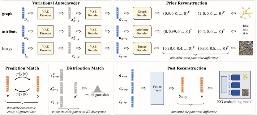
Figure 2: The workflow of GEEA. We use different sub-VAEs to process different sub-embeddings, and then use respective decoders to convert the sub-embeddings back to discrete features. Meanwhile, we reserve the entity alignment prediction loss, and use the latent variables of sub-VAEs for distribution match. The reconstructed sub-embeddings are also passed to the fusion layer in EEA model to produce the reconstructed joint embedding for post reconstruction.

3.4 Prior Reconstruction

We proposed prior reconstruction and the post reconstruction to fulfill our goal of generating entities with concrete features. The prior reconstruction aims to reconstruct the sub-embedding of each modal and recover the original concrete feature from the sub-embedding.

Take the relational graph information of flow $x\rightarrow y$ as an example, we first employs a sub-VAE to process the input sub-embedding:

$${\mathbf{g}}_{x\rightarrow y},{\mathbf{z}}_{x\rightarrow y}^{g}=\textit{VAE}_{g}({\mathbf{g}}_{x})$$ (18)

where $\textit{VAE}_{g}$ denote the variational autoencoder for relational graph information, ${\mathbf{g}}_{x}$ is the graph embedding of $x$, and ${\mathbf{g}}_{x\rightarrow y}$ is the reconstructed graph embedding for $y$ via $x$. ${\mathbf{z}}_{x\rightarrow y}^{g}$ is the corresponding latent variable.

We then recover the original features (i.e., the neighborhood information of $y$) by a prediction loss:

$$\mathcal{L}_{{\mathbf{g}}_{x\rightarrow y}}=g_{y}\log\textit{Decoder}_{g}({\mathbf{g}}_{x\rightarrow y})+(1-g_{y})\log(1-\textit{Decoder}_{g}({\mathbf{g}}_{x\rightarrow y})$$ (19)

$\mathcal{L}_{{\mathbf{g}}_{x\rightarrow y}}$ is a binary cross-entropy (BCE) loss, where we use a decoder $\textit{Decoder}_{g}$ to convert the reconstructed sub-embedding ${\mathbf{g}}_{x\rightarrow y}$ to a probability estimation about the neighborhood of $y$. For other modals and flows, we employ the similar methods to reconstruct the information, e.g., we recover the attribute information by predicting the attributes of an entity with the reconstructed sub-embedding as input. The details can be found in Appendix B.

3.5 Post Reconstruction

One potential problem is how to ensure that the reconstructed features of different modals belong to one entity. It is very likely to happen that these features do not match each other, even though the sub-VAEs produce desired outputs in their respective fields.

To avoid this issue, we propose post reconstruction, where we re-input the reconstructed sub-embeddings $\{{\mathbf{g}}_{x\rightarrow y},{\mathbf{a}}_{x\rightarrow y},...\}$ to the fusion layer (defined in the EEA model ${\mathcal{M}}$, see Figure 1) to obtain a reconstructed joint embedding ${\mathbf{y}}_{x\rightarrow y}$. We then employs a MSE loss to match the reconstructed joint embedding with the original one:

$${\mathbf{y}}_{x\rightarrow y} =\textit{Fusion}(\{{\mathbf{g}}_{x\rightarrow y},{\mathbf{a}}_{x\rightarrow y},...\}),\quad\forall(x,y)\in{\mathcal{S}}$$ (20)

$$\mathcal{L}_{x\rightarrow y} =\textit{MSE}({\mathbf{y}}_{x\rightarrow y},\textit{NoGradient}({\mathbf{y}})),\quad\forall(x,y)\in{\mathcal{S}},$$ (21)

where $\mathcal{L}_{x\rightarrow y}$ denotes the post reconstruction loss for the reconstructed joint embedding ${\mathbf{y}}_{x\rightarrow y}$. Fusion denotes the fusion layer in ${\mathcal{M}}$. MSE denotes the mean square error, in which we use the copy value of the original joint embedding $\textit{NoGradient}({\mathbf{y}})$ to avoid ${\mathbf{y}}$ inversely match ${\mathbf{y}}_{x\rightarrow y}$.

3.6 Implementation Details

We take Figure 2 as an example to illustrate the workflow of GEEA. First, the sub-embeddings outputted by ${\mathcal{M}}$ are taken as input for sub-VAEs (top-left). Then, the reconstructed sub-embeddings are passed to respective decoders to predict the discrete features of different modals (top-right). The conventional entity alignment prediction loss is also preserved in GEEA (bottom-left). The latent variables outputted by sub-VAEs are further used to match the distributions of predefined normal distribution (bottom-center). The reconstructed sub-embeddings are passed to the fusion layer to obtain a reconstructed joint embedding, which is used to match the true joint embedding for post reconstruction (bottom-right). The final training loss is:

$$\mathcal{L}=\underbrace{\sum_{f\in{\mathcal{F}}}\Big{(}\underbrace{\sum_{m\in\{g,a,i,...\}}\mathcal{L}_{{\mathbf{m}}_{f}}}_{\text{prior reconstruction}}+\underbrace{\mathcal{L}_{f}}_{\text{post reconstruction}}\Big{)}}_{\text{reconstruction term}}+\underbrace{\sum_{m\in\{g,a,i,...\}}\mathcal{L}_{\text{kld},m}}_{\text{distribution matching term}}+\underbrace{\mathcal{L}_{\text{ns}}}_{\text{prediction matching term}}$$ (22)

where ${\mathcal{F}}=\{x\rightarrow x,y\rightarrow y,x\rightarrow y,y\rightarrow x\}$ is the set of all flows and $\{g,a,i,...\}$ denotes the set of all available modals.

Table 1: Entity alignment results on DBP15K datasets, without surface information and iterative strategy. $\uparrow$: higher is better; $\downarrow$: lower is better. Average of $5$ runs, the same below.

Models	DBP15K${}_{\text{ZH-EN}}$			DBP15K${}_{\text{JA-EN}}$			DBP15K${}_{\text{FR-EN}}$
	Hits@1$\uparrow$	Hits@10$\uparrow$	MRR$\uparrow$	Hits@1$\uparrow$	Hits@10$\uparrow$	MRR$\uparrow$	Hits@1$\uparrow$	Hits@10$\uparrow$	MRR$\uparrow$
MUGNN [4]	.494	.844	.611	.501	.857	.621	.495	.870	.621
AliNet [6]	.539	.826	.628	.549	.831	.645	.552	.852	.657
decentRL [7]	.589	.819	.672	.596	.819	.678	.602	.842	.689
EVA [14]	.680	.910	.762	.673	.908	.757	.683	.923	.767
MSNEA [15]	.601	.830	.684	.535	.775	.617	.543	.801	.630
MCLEA [16]	.715	.923	.788	.715	.909	.785	.711	.909	.782
GEEA	.761	.946	.827	.755	.953	.827	.776	.962	.844

Table 2: Results on FB15K-DB15K and FB15K-YAGO15K datasets.

Models	# Paras (M)	FB15K-DB15K			FB15K-YAGO15K
		Hits@1$\uparrow$	Hits@10$\uparrow$	MRR$\uparrow$	Hits@1$\uparrow$	Hits@10$\uparrow$	MRR$\uparrow$
EVA	10.2	.199	.448	.283	.153	.361	.224
MSNEA	11.5	.114	.296	.175	.103	.249	.153
MCLEA	13.2	.295	.582	.393	.254	.484	.332
GEEA${}_{\text{SMALL}}$	11.2	.322	.602	.417	.270	.513	.352
GEEA	13.9	.343	.661	.450	.298	.585	.393

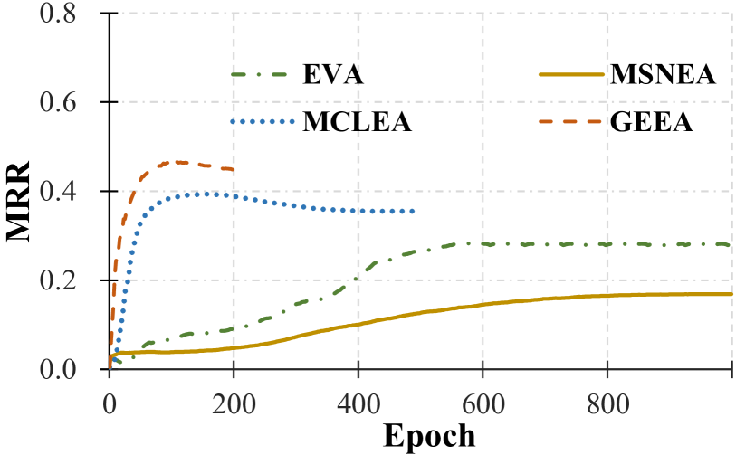
Figure 3: MRR results on FBDB15K, w.r.t. epochs.

4 Experiments

In this section, we conduct experiments to verify the effectiveness and efficiency of GEEA. The sourcecode and datasets have been uploaded and will be available on GitHub.

4.1 Settings

We used the popular multi-modal EEA benchmarks (DBP15K [2], FB15K-DB15K and FB15K-YAGO15K [13]) as datasets. Suggested by [19], we did not use the surface information which may lead to data leakage. The baselines MUGNN [4], AliNet [6] and decentRL [7] are methods tailored to relational graphs, while EVA [14], MSNEA [15] and MCLEA [16] are the multi-modal EEA methods which have achieved new state-of-the-art. We chose MCLEA [16] as the EEA model of GEEA in the main experiments. The results of using other models (e.g., EVA and MSNEA) can be found in Appendix C. For a fair comparison, the number of neural layers and dimensionality of input/hidden/output were set identical for all methods.

4.2 Entity Alignment Results

The entity alignment results on DBP15K are shown in Tables 1. We can observe that the multi-modal methods significantly outperformed the single-modal methods, demonstrating the strength of leveraging different resources. Remarkably, our GEEA achieved new state-of-the-art on all three datasets for all metrics. The superior performance empirically verified the correlations between the generative objectives and EEA objective.

4.3 Strengths and Weaknesses of GEEA on Entity Alignment

In Table 2, we compared the performance of the multi-modal methods on FB15K-DB15K and FB15K-YAGO15K where GEEA was still the best-performing method. Nevertheless, we observe that GEEA had more parameters compared with others, as it used VAEs and decoders to decode the embeddings back to concrete features. To probe the effectiveness of GEEA, we reduced the number of neurons to construct GEEA${}_{\text{SMALL}}$ and it still outperformed others with significant margin.

In Figure 3, we draw the curve of MRR results w.r.t. training epochs on FBDB15K, where we find that MCLEA and GEEA learned much faster than the methods with fewer parameters (i.e., EVA and MSNEA). In Figure 4, we further compared the performance of these two best-performing methods under different ratios of training alignment. We can observe that our GEEA achieved consistent better performance than MCLEA under various settings and metrics. We also find that the performance gap was more significantly when there were fewer training entity alignments ($\leq 30\%$). Overall, GEEA had more benefits than drawbacks, the additional parameters helped it learn faster and learn better.

Table 3: Entity synthesis results on five datasets. PRE ($\times 10^{-2}$), RE ($\times 10^{-2}$) denote the reconstruction errors for prior concrete features and output embeddings, respectively. FID [33] denotes Frechet Inception Distance for unconditional entity synthesis.

Models	DBP15K${}_{\text{ZH-EN}}$			DBP15K${}_{\text{JA-EN}}$			DBP15K${}_{\text{FR-EN}}$			FB15K-DB15K			FB15K-YAGO15K
	PRE$\downarrow$	RE$\downarrow$	FID$\downarrow$	PRE$\downarrow$	RE$\downarrow$	FID$\downarrow$	PRE$\downarrow$	RE$\downarrow$	FID$\downarrow$	PRE$\downarrow$	RE$\downarrow$	FID$\downarrow$	PRE$\downarrow$	RE$\downarrow$	FID$\downarrow$
MCLEA + decoder	8.104	4.218	N/A	7.640	5.441	N/A	10.578	5.985	N/A	18.504	$\inf$	N/A	20.997	$\inf$	N/A
VAE + decoder	0.737	0.206	1.821	0.542	0.329	2.184	0.856	0.689	3.083	10.564	11.354	10.495	9.645	9.982	16.180
Sub-VAEs + decoder	0.701	0.246	1.920	0.531	0.291	2.483	0.514	0.663	2.694	3.557	15.589	4.340	2.424	5.576	5.503
GEEA	0.438	0.184	0.935	0.385	0.195	1.871	0.451	0.121	2.422	3.141	6.151	3.089	1.730	2.039	3.903

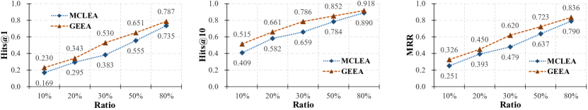
Figure 4: Entity alignment results on FBDB15K, w.r.t. ratios of training alignment.

4.4 Entity Synthesis Results

We modified the existing EEA benchmarks for entity synthesis experiments. Briefly, for each dataset, we randomly chose 30% of source entities in the testing alignment set as the dangling entities, and remove all the information of their counterpart entities during training. The goal is to reconstruct the information of their counterpart entities. We set the prior reconstruction error (for concrete features), reconstruction error (for embeddings), and Frechet Inception Distance (for unconditional synthesis) [33] as metrics. More details can be found in Appendix B.

The results are shown in Table 3. We also implemented several baselines for comparison: the EEA method MCLEA with our decoder performed worst in this experiment and it cannot generate new entities unconditionally. The performance of using Sub-VAEs to process different modals was usually better than that of using one VAE to process all embeddings, but we find that Sub-VAEs sometimes failed to reconstruct the embedding (e.g., the RE results on FB15K-DB15K). By contrast, our GEEA consistently and significantly outperformed these baselines. We also noticed the results on FB15K-DB15K and FB15K-YAGO15K were worse than those on DBP15K, which may be because the heterogeneity between two KGs is usually larger than that between two languages of one KG.

4.5 Case Study

We present some generated samples of GEEA conditioned on the source dangling entities in Table 4. Specifically, GEEA not only generated samples with the exact information that existed in the target KG, but also completed the target entities with highly reliable predictions. For example, the entity Star Wars (film) in target KG only had three basic attributes in the target KG, but GEEA predicted that it may also have the attributes like imdbid and initial release data.

Table 4: Entity synthesis samples from the FB15K-DB15K dataset. Since the image features are pretrained embeddings of a vision model, we use the image corresponded to the nearest neighbor of the reconstructed feature as the output image. The boldfaced denotes the exactly matched entry, while the underlined denotes the potentially true entry. More samples can be found in Appendix C.

Source		Target			GEEA Output
Entity	Image	Image	Neighborhood	Attribute	Image	Neighborhood	Attribute
Star Wars (film)			20th Century Fox, George Lucas, John Williams	runtime, gross, budget		20th Century Fox, George Lucas, Star Wars: Episode II, Willow (film), Aliens (film), Star Wars: The Clone War	initial release date, runtime, budget, gross, imdbId, numberOfEpisodes
Charles Darwin (naturalist)			Evolution, Australia, Royal Medal, Sigmund Freud	birthDate, deathDate		Royal Society, University of Cambridge, Royal Medal, Sigmund Freud, Austrians, Evolution	deathDate, birthDate, deathYear, birthYear, date of burial, height
George Harrison (musician)			The Beatles, Guitar, Rock music, Klaus Voormann, Jeff Lynne, Pop music	birthDate, deathDate, activeYearsStartYear, activeYearsEndYear, imdbId		The Beatles, The Band, Ringo Starr, Klaus Voormann, Jeff Lynne, Rock music	deathYear, birthYear, deathDate, birthDate, activeYearsStartYear, activeYearsEndYear, imdbId, height, networth

4.6 Ablation Study

We conducted ablation study to verify the effectiveness of each modules in GEEA in different tasks. In Table 5, we can observe that the best results was achieved by a complete GEEA and removing any module would result in performance loss in both two tasks. Interestingly, GEEA still learned some entity alignment information even we did not employ an EEA loss (the $2$nd row), which empirically proved that generative objectives helps EEA learning.

Table 5: Ablation study results on DBP15K${}_{\text{ZH-EN}}$.

Prediction	Distribution	Prior	Post	Entity Alignment			Entity Synthesis
Match	Match	Reconstruction	Reconstruction	Hits@1$\uparrow$	Hits@10$\uparrow$	MRR$\uparrow$	PRE$\downarrow$	RE$\downarrow$	FID$\downarrow$
$\surd$	$\surd$	$\surd$	$\surd$	.761	.946	.827	0.438	0.184	0.935
	$\surd$	$\surd$	$\surd$	.045	.186	.095	0.717	0.306	2.149
$\surd$		$\surd$	$\surd$	.702	.932	.783	0.551	0.193	1.821
$\surd$	$\surd$		$\surd$	.746	.930	.813	$\inf$	0.267	1.148
$\surd$	$\surd$	$\surd$		.750	.942	.819	0.701	0.246	1.920

5 Related Works

We split the related works into two categories:

Embedding-based Entity Alignment

Most pioneer works focus on modeling the relational graph information. According to the input form, they can be divided into triplet-based [1, 2, 9, 34, 35, 36] and GNN-based [4, 5, 6, 7, 37, 38]. The following works extend EEA with iterative training strategies which iteratively add new plausible aligned pairs as training data [8, 39, 40, 41]. We refer interested reader to surveys [18, 19]. Recent methods start to leverage multi-modal KG embedding for EEA [12, 13, 14, 15, 16, 17]. Although GEEA is based on multi-modal EEA models, it is not too relevant to them as it focuses on the objective optimization which is free of specific models. In this sense, the recent GAN-based methods [9, 10, 11] are closely related to GEEA but distinct from it. Specifically, all the existing methods are designed for single-modal EEA and aim to process the relational graph information in a fine-grained fashion. For example, NeoEA [11] proposed to align the conditional embedding distributions between two KGs, where the input variables are the entity embeddings conditioned on the relation embeddings they connect. If necessary, there is no contradiction to employ them to process relational graph information in GEEA. Another difference is the existing works do not consider the reconstruction process either for the embedding or the concrete feature. Their objective may be incomplete as illustrate in Section 2.

Variational Autoencoder

We draw the inspiration from many excellent works, e.g., VAEs, flow-based models, GANs, and diffusion models that have achieved state-of-the-art performance in many fields [33, 42, 43, 44, 45, 46]. Furthermore, recent studies [47, 48, 49, 50] find that these generative models can be used in controllable text generation. For example, Diffusion-LM [50] proposes a new language model that takes a sequence of Gaussian noise vectors as input and denoises them into a sentence of discrete words. To the best of our knowledge, GEEA is the first method capable of generating new entities with concrete features conditionally/unconditionally. The design of M-VAE, prior and post reconstruction is also different from existing generative models and may shed light on other fields.

6 Conclusion and Limitations

In this paper, we theoretically analyze how generative models can benefit EEA learning and propose GEEA to tackle the potential issues in existing methods. Our experiments demonstrate that GEEA can achieve state-of-the-art performance on both entity alignment and entity synthesis tasks. Currently, the main limitation is that GEEA employs the existing EEA models to encode different features, where they choose to replace some raw features (e.g., images) by the pretrained embeddings for efficiency and simplicity. However, this will hurt the generative capacity of GEEA to some extent. We plan to design new multi-modal EEA models to mitigate this problem in future work.

Appendix A Proofs of Things

A.1 The Complete Proof of Proposition 1

Proof.

Let $x\sim{\mathcal{X}}$, $y\sim{\mathcal{Y}}$ be two entities sampled from the entity sets ${\mathcal{X}}$, ${\mathcal{Y}}$, respectively. The main target of EEA is to learn a predictor to predict the conditional probability $p_{\theta}({\mathbf{x}}|{\mathbf{y}})$ (and reversely $p_{\theta}({\mathbf{y}}|{\mathbf{x}})$), where $\theta$ is the parameter set. For simplicity, we assume that the reverse function $p_{\theta}({\mathbf{y}}|{\mathbf{x}})$ shares this parameter set with $p_{\theta}({\mathbf{x}}|{\mathbf{y}})$.

Now, suppose that one wants to learn a generative model to generate entity embeddings:

$$\log p({\mathbf{x}}) =\log p({\mathbf{x}})\int p_{\theta}({\mathbf{y}}|{\mathbf{x}})d{\mathbf{y}}$$ (23)

$$=\int p_{\theta}({\mathbf{y}}|{\mathbf{x}})\log p({\mathbf{x}})d{\mathbf{y}}$$ (24)

$$=\mathbb{E}_{p_{\theta}({\mathbf{y}}|{\mathbf{x}})}[\log p({\mathbf{x}})]$$ (25)

$$=\mathbb{E}_{p_{\theta}({\mathbf{y}}|{\mathbf{x}})}\Big{[}\log\frac{p({\mathbf{x}},{\mathbf{y}})}{p({\mathbf{y}}|{\mathbf{x}})}\Big{]}$$ (26)

$$=\mathbb{E}_{p_{\theta}({\mathbf{y}}|{\mathbf{x}})}\Big{[}\log\frac{p({\mathbf{x}},{\mathbf{y}})p_{\theta}({\mathbf{y}}|{\mathbf{x}})}{p({\mathbf{y}}|{\mathbf{x}})p_{\theta}({\mathbf{y}}|{\mathbf{x}})}\Big{]}$$ (27)

$$=\mathbb{E}_{p_{\theta}({\mathbf{y}}|{\mathbf{x}})}\Big{[}\log\frac{p({\mathbf{x}},{\mathbf{y}})}{p_{\theta}({\mathbf{y}}|{\mathbf{x}})}\Big{]}+\mathbb{E}_{p_{\theta}({\mathbf{y}}|{\mathbf{x}})}\Big{[}\log\frac{p_{\theta}({\mathbf{y}}|{\mathbf{x}})}{p({\mathbf{y}}|{\mathbf{x}})}\Big{]}$$ (28)

$$=\mathbb{E}_{p_{\theta}({\mathbf{y}}|{\mathbf{x}})}\Big{[}\log\frac{p({\mathbf{x}},{\mathbf{y}})}{p_{\theta}({\mathbf{y}}|{\mathbf{x}})}\Big{]}+D_{\mathrm{KL}}(p_{\theta}({\mathbf{y}}|{\mathbf{x}})\parallel p({\mathbf{y}}|{\mathbf{x}})),$$ (29)

where the left hand of Equation (4) is usually called ELBO [25], and the right hand is the KL divergence [26] between our parameterized distribution $p_{\theta}({\mathbf{y}}|{\mathbf{x}})$ (i.e.,the predictor) and the true distribution $p({\mathbf{y}}|{\mathbf{x}})$. The complete derivation can be found in Appendix A.

The recent GAN-based methods [9, 10, 11] propose to leverage the entities out of training set for unsupervised learning. Their common idea is to make the entity embeddings from different KGs indiscriminative to a discriminator, and the underlying aligned entities shall be encoded in the same way and have similar embeddings. To formally prove this idea, we dissect the ELBO in Equation (4) as follows:

$$\mathbb{E}_{p_{\theta}({\mathbf{y}}|{\mathbf{x}})}\Big{[}\log\frac{p({\mathbf{x}},{\mathbf{y}})}{p_{\theta}({\mathbf{y}}|{\mathbf{x}})}\Big{]} =\mathbb{E}_{p_{\theta}({\mathbf{y}}|{\mathbf{x}})}\Big{[}\log\frac{p_{\theta}({\mathbf{x}}|{\mathbf{y}})p({\mathbf{y}})}{p_{\theta}({\mathbf{y}}|{\mathbf{x}})}\Big{]}$$ (30)

$$=\mathbb{E}_{p_{\theta}({\mathbf{y}}|{\mathbf{x}})}\Big{[}\log p_{\theta}({\mathbf{x}}|{\mathbf{y}})\Big{]}+\mathbb{E}_{p_{\theta}({\mathbf{y}}|{\mathbf{x}})}\Big{[}\log\frac{p({\mathbf{y}})}{p_{\theta}({\mathbf{y}}|{\mathbf{x}})}\Big{]}$$ (31)

$$=\mathbb{E}_{p_{\theta}({\mathbf{y}}|{\mathbf{x}})}\Big{[}\log p_{\theta}({\mathbf{x}}|{\mathbf{y}})\Big{]}-D_{\mathrm{KL}}(p_{\theta}({\mathbf{y}}|{\mathbf{x}})\parallel p({\mathbf{y}}))$$ (32)

Therefore, we have:

$$\log p({\mathbf{x}})=\underbrace{\vphantom{\mathbb{E}_{p_{\theta}({\mathbf{y}}|{\mathbf{x}})}\Big{[}\log p_{\theta}({\mathbf{x}}|{\mathbf{y}})\Big{]}}\mathbb{E}_{p_{\theta}({\mathbf{y}}|{\mathbf{x}})}\Big{[}\log p_{\theta}({\mathbf{x}}|{\mathbf{y}})\Big{]}}_{\text{reconstruction term}}-\underbrace{\vphantom{\mathbb{E}_{p_{\theta}({\mathbf{y}}|{\mathbf{x}})}\Big{[}\log p_{\theta}({\mathbf{x}}|{\mathbf{y}})\Big{]}}D_{\mathrm{KL}}(p_{\theta}({\mathbf{y}}|{\mathbf{x}})\parallel p({\mathbf{y}}))}_{\text{distribution matching term}}+\underbrace{\vphantom{\mathbb{E}_{p_{\theta}({\mathbf{y}}|{\mathbf{x}})}\Big{[}\log p_{\theta}({\mathbf{x}}|{\mathbf{y}})\Big{]}}D_{\mathrm{KL}}(p_{\theta}({\mathbf{y}}|{\mathbf{x}})\parallel p({\mathbf{y}}|{\mathbf{x}}))}_{\text{prediction matching term}}$$ (33)

The first term aims to reconstruct the original embedding ${\mathbf{x}}$ based on ${\mathbf{y}}$ generated from ${\mathbf{x}}$, which has not been studied by the existing EEA works. The second term imposes the distribution ${\mathbf{y}}$ conditioned on ${\mathbf{x}}$ to match the prior distribution of ${\mathbf{y}}$, which has been investigated by the GAN-based EEA methods [9, 10, 11]. The third term is the main objective of EEA (i.e., Equation (5) where the target $p({\mathbf{y}}|{\mathbf{x}})$ is partly observed).

Note that, $p({\mathbf{x}})$ is irrelevant to our parameter set $\theta$ and thus can be regarded as a constant during optimization. Therefore, maximizing the ELBO (i.e., maximizing the first term and minimizing the second term) will result in minimizing the third term, concluding the proof. ∎

A.2 Proof of Proposition 2

Proof.

We first have a look on the right hand:

$$D_{\mathrm{KL}}(p({{\mathbf{z}}_{x\rightarrow x}}),p({\mathbf{z}}^{*}))+D_{\mathrm{KL}}(p({{\mathbf{z}}_{y\rightarrow y}}),p({\mathbf{z}}^{*}))$$ (34)

Ideally, all the variables ${\mathbf{z}}_{x\rightarrow x}$, ${\mathbf{z}}_{y\rightarrow y}$, and ${\mathbf{z}}^{*}$ follow the Gaussian distributions with $\mu_{x\rightarrow x}$, $\mu_{y\rightarrow y}$, $\mu^{*}$ and $\sigma_{x\rightarrow x}$, $\sigma_{y\rightarrow y}$, $\sigma^{*}$ as mean and variance, respectively.

Luckily, we can use the following equation to calculate the KL divergence between two Gaussian distributions conveniently:

$$D_{\mathrm{KL}}(p({\mathbf{z}}_{1}),p({\mathbf{z}}_{2}))=\log\frac{\sigma_{2}}{\sigma_{1}}+\frac{\sigma_{1}^{2}+(\mu_{1}-\mu_{2})^{2}}{2\sigma^{2}_{2}}-\frac{1}{2},$$ (35)

and rewrite Equation(34 as:

$$D_{\mathrm{KL}}(p({{\mathbf{z}}_{x\rightarrow x}}),p({\mathbf{z}}^{*}))+D_{\mathrm{KL}}(p({{\mathbf{z}}_{y\rightarrow y}}),p({\mathbf{z}}^{*}))$$ (36)

$$= (\log\frac{\sigma^{*}}{\sigma_{x\rightarrow x}}+\frac{\sigma_{x\rightarrow x}^{2}+(\mu_{x\rightarrow x}-\mu^{*})^{2}}{2(\sigma^{*})^{2}}-\frac{1}{2})+(\log\frac{\sigma^{*}}{\sigma_{y\rightarrow y}}+\frac{\sigma_{y\rightarrow y}^{2}+(\mu_{y\rightarrow y}-\mu^{*})^{2}}{2(\sigma^{*})^{2}}-\frac{1}{2})$$ (37)

$$= (\log\frac{\sigma^{*}}{\sigma_{x\rightarrow x}}+\log\frac{\sigma^{*}}{\sigma_{y\rightarrow y}})+(\frac{\sigma_{x\rightarrow x}^{2}+(\mu_{x\rightarrow x}-\mu^{*})^{2}}{2(\sigma^{*})^{2}}+\frac{\sigma_{y\rightarrow y}^{2}+(\mu_{y\rightarrow y}-\mu^{*})^{2}}{2(\sigma^{*})^{2}})-1$$ (38)

$$= (\log\frac{\sigma^{*}}{\sigma_{x\rightarrow x}}+\log\frac{\sigma^{*}}{\sigma_{y\rightarrow y}})+\frac{\sigma_{x\rightarrow x}^{2}+(\mu_{x\rightarrow x}-\mu^{*})^{2}+\sigma_{y\rightarrow y}^{2}+(\mu_{y\rightarrow y}-\mu^{*})^{2}}{2(\sigma^{*})^{2}}-1$$ (39)

$$= (\log$$ (40)

Take ${\mathbf{z}}^{*}\sim{\mathcal{N}}(\mu^{*}=\mathbf{0},\sigma^{*}={\mathbf{I}})$ into the above equation, we will have:

$$D_{\mathrm{KL}}(p({{\mathbf{z}}_{x\rightarrow x}}),p({\mathbf{z}}^{*}))+D_{\mathrm{KL}}(p({{\mathbf{z}}_{y\rightarrow y}}),p({\mathbf{z}}^{*}))$$ (41)

$$= -\log\sigma_{x\rightarrow x}\sigma_{y\rightarrow y}+\frac{1}{2}(\sigma_{x\rightarrow x}^{2}+\sigma_{y\rightarrow y}^{2}+\mu_{x\rightarrow x}^{2}+\mu_{y\rightarrow y}^{2})-1$$ (42)

Similarly, the left hand can be expanded as:

$$D_{\mathrm{KL}}(p({\mathbf{z}}_{x\rightarrow x}),p({\mathbf{z}}_{y\rightarrow y}))=\log\frac{\sigma_{y\rightarrow y}}{\sigma_{x\rightarrow x}}+\frac{\sigma_{x\rightarrow x}^{2}+(\mu_{x\rightarrow x}-\mu_{y\rightarrow y})^{2}}{2\sigma^{2}_{y\rightarrow y}}-\frac{1}{2},$$ (43)

Thus, the difference between the right hand and the right hand can be computed:

$$D_{\mathrm{KL}}(p({{\mathbf{z}}_{x\rightarrow x}}),p({\mathbf{z}}^{*}))+D_{\mathrm{KL}}(p({{\mathbf{z}}_{y\rightarrow y}}),p({\mathbf{z}}^{*}))-D_{\mathrm{KL}}(p({\mathbf{z}}_{x\rightarrow x}),p({\mathbf{z}}_{y\rightarrow y}))$$ (44)

$$= -\log\sigma_{x\rightarrow x}\sigma_{y\rightarrow y}+\frac{1}{2}(\sigma_{x\rightarrow x}^{2}+\sigma_{y\rightarrow y}^{2}+\mu_{x\rightarrow x}^{2}+\mu_{y\rightarrow y}^{2})-1$$ (45)

$$-(\log\frac{\sigma_{y\rightarrow y}}{\sigma_{x\rightarrow x}}+\frac{\sigma_{x\rightarrow x}^{2}+(\mu_{x\rightarrow x}-\mu_{y\rightarrow y})^{2}}{2\sigma^{2}_{y\rightarrow y}}-\frac{1}{2})$$ (46)

$$= (-\log\sigma_{x\rightarrow x}\sigma_{y\rightarrow y}-\log\frac{\sigma_{y\rightarrow y}}{\sigma_{x\rightarrow x}})$$ (47)

$$+(\frac{1}{2}(\sigma_{x\rightarrow x}^{2}+\sigma_{y\rightarrow y}^{2}+\mu_{x\rightarrow x}^{2}+\mu_{y\rightarrow y}^{2})-\frac{\sigma_{x\rightarrow x}^{2}+(\mu_{x\rightarrow x}-\mu_{y\rightarrow y})^{2}}{2\sigma^{2}_{y\rightarrow y}})+(-1+\frac{1}{2})$$ (48)

$$= -2\log\sigma_{y\rightarrow y}-\frac{1}{2}$$ (49)

$$+\frac{\sigma_{x\rightarrow x}^{2}\sigma_{y\rightarrow y}^{2}+\sigma_{y\rightarrow y}^{4}+\mu_{x\rightarrow x}^{2}\sigma_{y\rightarrow y}^{2}+\mu_{y\rightarrow y}^{2}\sigma_{y\rightarrow y}^{2}-\sigma_{x\rightarrow x}^{2}-\mu_{x\rightarrow x}^{2}-\mu_{y\rightarrow y}^{2}+2\mu_{x\rightarrow x}\mu_{y\rightarrow y}}{2\sigma^{2}_{y\rightarrow y}}$$ (50)

$$= -2\log\sigma_{y\rightarrow y}-\frac{1}{2}$$ (51)

$$+\frac{(\sigma_{y\rightarrow y}^{2}-1)\sigma_{x\rightarrow x}^{2}+(\mu_{x\rightarrow x}^{2}+\mu_{y\rightarrow y}^{2})(\sigma_{y\rightarrow y}^{2}-1)+\sigma_{y\rightarrow y}^{4}+2\mu_{x\rightarrow x}\mu_{y\rightarrow y}}{2\sigma^{2}_{y\rightarrow y}}$$ (52)

$$= -2\log\sigma_{y\rightarrow y}-\frac{1}{2}+\frac{(\mu_{x\rightarrow x}^{2}+\mu_{y\rightarrow y}^{2}+\sigma_{x\rightarrow x}^{2})(\sigma_{y\rightarrow y}^{2}-1)+\sigma_{y\rightarrow y}^{4}+2\mu_{x\rightarrow x}\mu_{y\rightarrow y}}{2\sigma^{2}_{y\rightarrow y}}$$ (53)

As we optimize ${\mathbf{z}}_{y\rightarrow y}\rightarrow{\mathbf{z}}^{*}$, i.e., minimize $D_{\mathrm{KL}}(p({{\mathbf{z}}_{y\rightarrow y}}),p({\mathbf{z}}^{*}))$, we will have:

$$\log\sigma_{y\rightarrow y}\rightarrow 0,\quad\sigma_{y\rightarrow y}^{2}-1\rightarrow 0,\quad\mu_{x\rightarrow x}\mu_{y\rightarrow y}\rightarrow 0,\quad\sigma_{y\rightarrow y}^{4}\rightarrow 1,$$ (54)

and consequently:

$$D_{\mathrm{KL}}(p({{\mathbf{z}}_{x\rightarrow x}}),p({\mathbf{z}}^{*}))+D_{\mathrm{KL}}(p({{\mathbf{z}}_{y\rightarrow y}}),p({\mathbf{z}}^{*}))-D_{\mathrm{KL}}(p({\mathbf{z}}_{x\rightarrow x}),p({\mathbf{z}}_{y\rightarrow y}))\rightarrow 0,$$ (55)

Similarly, as we optimize ${\mathbf{z}}_{x\rightarrow x}\rightarrow{\mathbf{z}}^{*}$, i.e., minimize $D_{\mathrm{KL}}(p({{\mathbf{z}}_{x\rightarrow x}}),p({\mathbf{z}}^{*}))$, we will have:

$$D_{\mathrm{KL}}(p({{\mathbf{z}}_{x\rightarrow x}}),p({\mathbf{z}}^{*}))+D_{\mathrm{KL}}(p({{\mathbf{z}}_{y\rightarrow y}}),p({\mathbf{z}}^{*}))-D_{\mathrm{KL}}(p({\mathbf{z}}_{y\rightarrow y}),p({\mathbf{z}}_{x\rightarrow x}))\rightarrow 0$$ (56)

Therefore, jointly minimizing $D_{\mathrm{KL}}(p({{\mathbf{z}}_{x\rightarrow x}}),p({\mathbf{z}}^{*}))$ and $D_{\mathrm{KL}}(p({{\mathbf{z}}_{y\rightarrow y}}),p({\mathbf{z}}^{*}))$ will subsequently minimizing $D_{\mathrm{KL}}(p({\mathbf{z}}_{x\rightarrow x}),p({\mathbf{z}}_{y\rightarrow y}))$ and $D_{\mathrm{KL}}(p({\mathbf{z}}_{y\rightarrow y}),p({\mathbf{z}}_{x\rightarrow x}))$, and finally aligning the distributions between ${\mathbf{x}}$ and ${\mathbf{y}}$, concluding the proof. ∎

Appendix B Implementation Details

B.1 Decoding Embeddings back to Concrete Features

All decoders used to decode the reconstructed embeddings to the concrete features comprise several hidden layers and an output layer. Specifically, each hidden layer has a linear layer with layer norm and ReLU/Tanh activations. The output layer is different for different modals. For the relational graph and attribute information, their concrete features are organized in the form of multi-classification labels. For example, the relational graph information $g_{i}$ for and entity $x_{i}$ is represented by:

$$g_{i}=(0,...,1,...1,...,0)^{T},\quad|g_{i}|=|{\mathcal{X}}|,$$ (57)

where $g_{i}$ has $|{\mathcal{X}}|$ elements where $1$ indicates the connection and $0$ otherwise. Therefore, the output layer transforms the hidden output to the concrete feature prediction with a matrix $W_{o}\in\mathbb{R}^{H\times|{\mathcal{X}}|}$, where $H$ is the output dimension of the final hidden layer.

The image concrete features are actually the pretrained embeddings rather than pixel data, as we use the existing EEA models for embedding entities. Therefore, we replaced the binary cross-entropy loss by a MSE loss to train GEEA to recover this pretrained embedding.

B.2 Implementing a GEEA

We implement GEEA with PyTorch and run the main experiments on a RTX 4090. We illustrate the training procedure of GEEA by Algorithm 1. We first initialize all trainable varibles and the get the mini-batch data of supervised flows $x\rightarrow y$, $y\rightarrow x$ and unsupervised flows $x\rightarrow x$, $y\rightarrow y$, respectively.

For the supervised flows, we iterate the batched data and calculate the prediction matching loss which is also used in most existing works. Then, we calculate the distribution matching, prior reconstruction and post reconstruction losses and sum it for later joint optimization.

For the unsupervised flows, we first process the raw feature with ${\mathcal{M}}$ and VAE to obtain the embeddings and reconstructed embeddings. Then we estimate the distribution matching loss with the embedding sets as input (Equation (16)), after which we calculate the prior and post reconstruction loss for each $x$ and each $y$.

Finally, we sum all the losses produced with the all flows, and minimize them until the performance on the valid dataset dose not improve.

The overall hyper-parameter settings in the main experiments are presented in Table 6.

Algorithm 1 Generative Embedding-based Entity Alignment

1:  Input: The entity sets ${\mathcal{X}}$, ${\mathcal{Y}}$, the multi-modal information ${\mathcal{G}}$, ${\mathcal{A}}$, ${\mathcal{I}}$ …, the EEA model ${\mathcal{M}}$, and M-VAE VAE;

2:  Randomly initialize all parameters;

3:  repeat

4:     ${\mathcal{B}}_{\text{sup}}\leftarrow\{(x,y)|(x,y)\sim{\mathcal{S}}\}$;  // get a batch of supervised training data

5:     ${\mathcal{B}}_{\text{unsup}}\leftarrow\{(x,y)|x\sim{\mathcal{X}},y\sim{\mathcal{Y}}\}$;  // get a batch of unsupervised training data

6:     for $(x,y)\in{\mathcal{B}}_{\text{sup}}$ do

7:        ${\mathbf{x}},{\mathbf{y}}\leftarrow{\mathcal{M}}(x),{\mathcal{M}}(y)$;  // obtain embeddings and sub-embeddings

8:        ${\mathbf{y}}_{x\rightarrow y},{\mathbf{x}}_{y\rightarrow x}\leftarrow\textit{VAE}({\mathbf{x}}),\textit{VAE}({\mathbf{y}})$;  // obtain the reconstructed mutual embeddings

9:        Calculate the prediction matching loss following Equation (5);

10:        Calculate the prior reconstruction loss following Equation (19);

11:        Calculate the post reconstruction loss following Equation (20);

12:     end for

13:     $\{{\mathbf{x}}_{x\rightarrow x},{\mathbf{y}}_{y\rightarrow y}|(x,y)\in{\mathcal{B}}_{\text{unsup}}\}\leftarrow\{\textit{VAE}({\mathcal{M}}(x)),\textit{VAE}({\mathcal{M}}(y))|(x,y)\in{\mathcal{B}}_{\text{unsup}}\}$; // obtain the reconstructed self embeddings

14:     Calculate the distribution matching loss following Equation (16);

15:     Calculate the prior reconstruction loss following Equation (19);

16:     Calculate the post reconstruction loss following Equation (20);

17:     Jointly minimize all losses;

18:  until the performance does not improve.

Table 6: Hyper-parameter settings in the main experiments.

Datasets	# epoch	batch-size	# VAE layers	learning rate	optimizer	dropout rate	# unsupervised batch-size	flow weights (xx,yy,xy,yx)	loss weights (DM, PrioR, PostR)	# hidden sizes	latent size	decoder hidden sizes
DBP15K${}_{\text{ZH-EN}}$	200	2,500	2	0.001	Adam	0.5	2,800	[1.,1.,5.,5.]	[0.5,1,1]	[300,300]	300	[300,1000]
DBP15K${}_{\text{JA-EN}}$	200	2,500	2	0.001	Adam	0.5	2,800	[1.,1.,5.,5.]	[0.5,1,1]	[300,300]	300	[300,1000]
DBP15K${}_{\text{FR-EN}}$	200	2,500	2	0.001	Adam	0.5	2,800	[1.,1.,5.,5.]	[0.5,1,1]	[300,300]	300	[300,1000]
FB15K-DB15K	300	3,500	3	0.0005	Adam	0.5	2,500	[1.,1.,5.,5.]	[0.5,1,1]	[300,300,300]	300	[300,300,1000]
FB15K-YAGO15K	300	3,500	3	0.0005	Adam	0.5	2,500	[1.,1.,5.,5.]	[0.5,1,1]	[300,300,300]	300	[300,300,1000]

Appendix C Additional Experiments

Table 7: Statistics of the datasets.

Datasets	Entity Alignment	Entity Synthesis		# Entities	# Relations	# Attributes	# Images
	# Test Alignments	# Known Test Alignments	# Unknown Test Alignments
DBP15K${}_{\text{ZH-EN}}$	10,500	7,350	3,150	19,388	1,701	8,111	15,912
	10,500	7,350	3,150	19,572	1,323	7,173	14,125
DBP15K${}_{\text{JA-EN}}$	10,500	7,350	3,150	19,814	1,299	5,882	12,739
	10,500	7,350	3,150	19,780	1,153	6,066	13,741
DBP15K${}_{\text{FR-EN}}$	10,500	7,350	3,150	19,661	903	4,547	14,174
	10,500	7,350	3,150	19,993	1,208	6,422	13,858
FB15K-DB15K	10,276	7,193	3,083	14,951	1,345	116	13,444
	10,500	7,350	3,150	12,842	279	225	12,837
FB15K-YAGO15K	8,959	6,272	2,687	14,951	1,345	116	13,444
	10,500	7,350	3,150	15,404	32	7	11,194

Table 8: Entity alignment results of GEEA with different EEA models on DBP15K datasets.

Models	DBP15K${}_{\text{ZH-EN}}$			DBP15K${}_{\text{JA-EN}}$			DBP15K${}_{\text{FR-EN}}$
	Hits@1$\uparrow$	Hits@10$\uparrow$	MRR$\uparrow$	Hits@1$\uparrow$	Hits@10$\uparrow$	MRR$\uparrow$	Hits@1$\uparrow$	Hits@10$\uparrow$	MRR$\uparrow$
EVA [14]	.680	.910	.762	.673	.908	.757	.683	.923	.767
GEEA w/ EVA	.715	.922	.794	.707	.925	.791	.727	.940	.817
MSNEA [15]	.601	.830	.684	.535	.775	.617	.543	.801	.630
GEEA w/ MSNEA	.643	.872	.732	.559	.821	.671	.586	.853	.672
MCLEA [16]	.715	.923	.788	.715	.909	.785	.711	.909	.782
GEEA w/ MCLEA	.761	.946	.827	.755	.953	.827	.776	.962	.844

Table 9: More entity synthesis samples from different dataset. The first two rows are from FB15K-YAGO15K; the middle two rows are from DBP15K${}_{\text{ZH-EN}}$; the last two rows are from DBP15K${}_{\text{FR-EN}}$.

Source		Target			GEEA Output
Entity	Image	Image	Neighborhood	Attribute	Image	Neighborhood	Attribute
James Cameron (director)			United States, New Zealand, Kathryn Bigelow, Avatar (2009 film), The Terminator	wasBornOnDate		Kathryn Bigelow, United States, The Terminator, Jonathan Frakes, James Cameron	wasBornOnDate, diedOnDate, diedOnDate
Northwest Territories (Canada)			Canada, English language, French language	wasCreatedOnDate, hasLatitude, hasLongitude		English language, Yukon, Nunavut, French language, Canada, Prince Edward Island	wasCreatedOnDate, hasLatitude, hasLongitude, wasDestroyedOnDate
苏州市 (Suzhou)			Lake Tai, Suzhou dialect, Jiangsu, Han Xue (actress), Wu Chinese	populationTotal, mapCaption, location, longd latd, populationUrban		Lake Tai, Suzhou dialect, Jiangsu, Han Xue (actress), Wu Chinese, Huzhou, Hangzhou, Jiangyin	mapCaption, populationTotal, location, longd, latd, populationUrban, populationDensityKm, areaTotalKm, postalCode
周杰伦 (Jay Chou)			Fantasy (Jay Chou album), Jay (album), The Era (album), Capricorn (Jay Chou album), Rock music, Pop music	name, birthDate, occupation, yearsactive birthPlace, awards		The Era (album), Capricorn (Jay Chou album), Jay (album), Fantasy (Jay Chou album), Pop music, Ye Hui Mei, Perfection (EP), Sony Music Entertainment	name, occupation, birthDate, yearsactive, birthPlace, awards, pinyinchinesename, spouse, children
Forel (Lavaux)			Puidoux, Essertes, Servion, Savigny, Switzerland	name, population, canton, population postalCode, languages		Servion, Puidoux, Essertes, Savigny, Switzerland, Montpreveyres, Corcelles-le-Jorat, Pully, Ropraz	name, canton, population, languages, légende, latitude, longitude, blason, gentilé
Nintendo 3DS			Nintendo, Kirby (series), Nintendo DS, Super Smash Bros., Yo-Kai Watch, Need for Speed	name, title, caption, logo		Nintendo, Kirby (series), Nintendo DS, Super Smash Bros., Yo-Kai Watch, Shigeru Miyamoto, Game Boy, Nintendo 64	name, title caption, date, type, trad, width, année, période

Table 10: Some false samples from FB15K-YAGO15K.

Source		Target			GEEA Output
Entity	Image	Image	Neighborhood	Attribute	Image	Neighborhood	Attribute
The Matrix (film)			Carrie-Anne Moss, Keanu Reeves, Laurence Fishburne Hugo Weaving	wasCreatedOnDate		District 9, What Lies Beneath, Avatar (2009 film), Ibad Muhamadu, The Fugitive (1993 film), Denny Landzaat, Michael Lamey, Dries Boussatta	wasBornOnDate, wasCreatedOnDate, diedOnDate
The Terminator (film)			United States, Michael Biehn, James Cameron Arnold Schwarzenegger	wasCreatedOnDate		United States, Nicaraguan Revolution, Ibad Muhamadu, José Rodrigues Neto, Anaconda (film)	wasCreatedOnDate, diedOnDate, wasCreatedOnDate, wasDestroyedOnDate,

C.1 Datasets

We present the statistics of entity alignment and entity synthesis datasets in Table 7. To construct an entity synthesis dataset, we first sample 30% of entity alignments from the testing set of the original entity alignment dataset. Then, we view the source entities in sampled entities pairs as the dangling entities, and make their target entities unseen during training. To this end, we remove all types of information referred to these target entities from training set.

C.2 GEEA with different EEA models

We also investigated the performance of GEEA with different EEA models. As shown in Table 8, GEEA significantly improved all the baseline models on all metrics and datasets. Remarkably, the performance of EVA with GEEA on some datasets like DBP15K${}_{\text{FR-EN}}$ were even better than that of the original MCLEA.

C.3 Results with Different Alignment Ratios on All Datasets

We present the results with different alignment ratios on all datasets in Figure 5, which demonstrate the same conclusion as in Figure 4.

C.4 More Entity Synthesis Samples

We illustrate more entity synthesis samples in Table 9 and some false samples in Table 10. The main reason for unpromising synthesis results is the lack of information. For example, in the FB15K-YAGO15K datasets, the YAGO KG only has $7$ different attributes. Also, as some entities do not have image features, the EEA models choose to initialize the pretrained image embeddings with random vectors. To mitigate this problem, we plan to design new benchmarks and new EEA models to directly process and generate the raw data in future work.

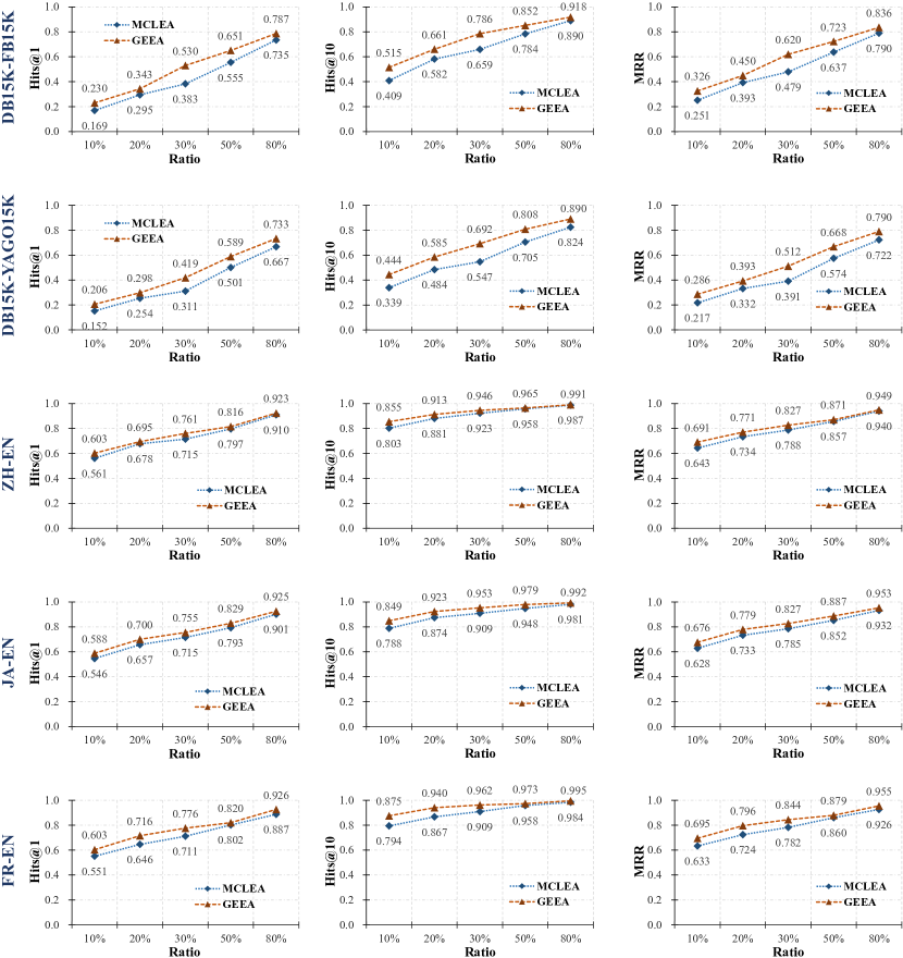
Figure 5: Entity alignment results on all datasets, w.r.t. ratios of training alignment.

References

- Chen et al. [2017] Muhao Chen, Yingtao Tian, Mohan Yang, and Carlo Zaniolo. Multilingual knowledge graph embeddings for cross-lingual knowledge alignment. In IJCAI, 2017.
- Sun et al. [2017] Zequn Sun, Wei Hu, and Chengkai Li. Cross-lingual entity alignment via joint attribute-preserving embedding. In ISWC, 2017.
- Sun et al. [2018] Zequn Sun, Wei Hu, Qingheng Zhang, and Yuzhong Qu. Bootstrapping entity alignment with knowledge graph embedding. In IJCAI, 2018.
- Cao et al. [2019] Yixin Cao, Zhiyuan Liu, Chengjiang Li, Zhiyuan Liu, Juanzi Li, and Tat-Seng Chua. Multi-channel graph neural network for entity alignment. In ACL, 2019.
- Wang et al. [2018] Zhichun Wang, Qingsong Lv, Xiaohan Lan, and Yu Zhang. Cross-lingual knowledge graph alignment via graph convolutional networks. In EMNLP, 2018.
- Sun et al. [2020a] Zequn Sun, Chengming Wang, Wei Hu, Muhao Chen, Jian Dai, Wei Zhang, and Yuzhong Qu. Knowledge graph alignment network with gated multi-hop neighborhood aggregation. In AAAI, 2020a.
- Guo et al. [2020] Lingbing Guo, Weiqing Wang, Zequn Sun, Chenghao Liu, and Wei Hu. Decentralized knowledge graph representation learning. CoRR, abs/2010.08114, 2020.
- Guo et al. [2022a] Lingbing Guo, Yuqiang Han, Qiang Zhang, and Huajun Chen. Deep reinforcement learning for entity alignment. In Smaranda Muresan, Preslav Nakov, and Aline Villavicencio, editors, Findings of ACL, pages 2754–2765, 2022a.
- Pei et al. [2019a] Shichao Pei, Lu Yu, Robert Hoehndorf, and Xiangliang Zhang. Semi-supervised entity alignment via knowledge graph embedding with awareness of degree difference. In WWW, pages 3130–3136, 2019a.
- Pei et al. [2019b] Shichao Pei, Lu Yu, and Xiangliang Zhang. Improving cross-lingual entity alignment via optimal transport. In IJCAI, pages 3231–3237, 2019b.
- Guo et al. [2022b] Lingbing Guo, Qiang Zhang, Zequn Sun, Mingyang Chen, Wei Hu, and Huajun Chen. Understanding and improving knowledge graph embedding for entity alignment. In Kamalika Chaudhuri, Stefanie Jegelka, Le Song, Csaba Szepesvári, Gang Niu, and Sivan Sabato, editors, ICML, volume 162, pages 8145–8156, 2022b.
- Zhang et al. [2019] Qingheng Zhang, Zequn Sun, Wei Hu, Muhao Chen, Lingbing Guo, and Yuzhong Qu. Multi-view knowledge graph embedding for entity alignment. In Sarit Kraus, editor, IJCAI, pages 5429–5435, 2019.
- Chen et al. [2020] Liyi Chen, Zhi Li, Yijun Wang, Tong Xu, Zhefeng Wang, and Enhong Chen. MMEA: entity alignment for multi-modal knowledge graph. In KSEM (1), volume 12274, pages 134–147, 2020.
- Liu et al. [2021] Fangyu Liu, Muhao Chen, Dan Roth, and Nigel Collier. Visual pivoting for (unsupervised) entity alignment. In AAAI, pages 4257–4266, 2021.
- Chen et al. [2022a] Liyi Chen, Zhi Li, Tong Xu, Han Wu, Zhefeng Wang, Nicholas Jing Yuan, and Enhong Chen. Multi-modal siamese network for entity alignment. In KDD, pages 118–126, 2022a.
- Lin et al. [2022] Zhenxi Lin, Ziheng Zhang, Meng Wang, Yinghui Shi, Xian Wu, and Yefeng Zheng. Multi-modal contrastive representation learning for entity alignment. In COLING, pages 2572–2584, 2022.
- Chen et al. [2022b] Zhuo Chen, Jiaoyan Chen, Wen Zhang, Lingbing Guo, Yin Fang, Yufeng Huang, Yuxia Geng, Jeff Z Pan, Wenting Song, and Huajun Chen. Meaformer: Multi-modal entity alignment transformer for meta modality hybrid. arXiv preprint arXiv:2212.14454, 2022b.
- Wang et al. [2017] Quan Wang, Zhendong Mao, Bin Wang, and Li Guo. Knowledge graph embedding: A survey of approaches and applications. IEEE Transactions on Knowledge and Data Engineering, 29, 2017.
- Sun et al. [2020b] Zequn Sun, Qingheng Zhang, Wei Hu, Chengming Wang, Muhao Chen, Farahnaz Akrami, and Chengkai Li. A benchmarking study of embedding-based entity alignment for knowledge graphs. CoRR, abs/2003.07743, 2020b.
- Sun et al. [2021] Zequn Sun, Muhao Chen, and Wei Hu. Knowing the no-match: Entity alignment with dangling cases. In Proceedings of the 59th Annual Meeting of the Association for Computational Linguistics and the 11th International Joint Conference on Natural Language Processing (Volume 1: Long Papers), pages 3582–3593, 2021.
- Luo and Yu [2022] Shengxuan Luo and Sheng Yu. An accurate unsupervised method for joint entity alignment and dangling entity detection. arXiv preprint arXiv:2203.05147, 2022.
- Liu et al. [2022] Juncheng Liu, Zequn Sun, Bryan Hooi, Yiwei Wang, Dayiheng Liu, Baosong Yang, Xiaokui Xiao, and Muhao Chen. Dangling-aware entity alignment with mixed high-order proximities. arXiv preprint arXiv:2205.02406, 2022.
- Khalifa et al. [2017] Ahmed Khalifa, Michael Cerny Green, Diego Perez-Liebana, and Julian Togelius. General video game rule generation. In CIG, pages 170–177, 2017.
- Lee et al. [2021] Lik-Hang Lee, Tristan Braud, Pengyuan Zhou, Lin Wang, Dianlei Xu, Zijun Lin, Abhishek Kumar, Carlos Bermejo, and Pan Hui. All one needs to know about metaverse: A complete survey on technological singularity, virtual ecosystem, and research agenda. arXiv preprint arXiv:2110.05352, 2021.
- Kingma and Welling [2013] Diederik P Kingma and Max Welling. Auto-encoding variational bayes. arXiv preprint arXiv:1312.6114, 2013.
- Kullback and Leibler [1951] Solomon Kullback and Richard A Leibler. On information and sufficiency. The annals of mathematical statistics, 22(1):79–86, 1951.
- Srivastava et al. [2017] Akash Srivastava, Lazar Valkov, Chris Russell, Michael U Gutmann, and Charles Sutton. Veegan: Reducing mode collapse in gans using implicit variational learning. NeurIPS, 30, 2017.
- Kingma et al. [2016] Durk P Kingma, Tim Salimans, Rafal Jozefowicz, Xi Chen, Ilya Sutskever, and Max Welling. Improved variational inference with inverse autoregressive flow. NeurIPS, 29, 2016.
- Sønderby et al. [2016] Casper Kaae Sønderby, Tapani Raiko, Lars Maaløe, Søren Kaae Sønderby, and Ole Winther. Ladder variational autoencoders. NeurIPS, 29, 2016.
- Ho et al. [2020a] Jonathan Ho, Ajay Jain, and Pieter Abbeel. Denoising diffusion probabilistic models. NeurIPS, 33:6840–6851, 2020a.
- Kingma et al. [2021] Diederik Kingma, Tim Salimans, Ben Poole, and Jonathan Ho. Variational diffusion models. NeurIPS, 34:21696–21707, 2021.
- Ho et al. [2022] Jonathan Ho, Chitwan Saharia, William Chan, David J Fleet, Mohammad Norouzi, and Tim Salimans. Cascaded diffusion models for high fidelity image generation. J. Mach. Learn. Res., 23:47–1, 2022.
- Heusel et al. [2017] Martin Heusel, Hubert Ramsauer, Thomas Unterthiner, Bernhard Nessler, and Sepp Hochreiter. Gans trained by a two time-scale update rule converge to a local nash equilibrium. In Isabelle Guyon, Ulrike von Luxburg, Samy Bengio, Hanna M. Wallach, Rob Fergus, S. V. N. Vishwanathan, and Roman Garnett, editors, NeurIPS, pages 6626–6637, 2017.
- Guo et al. [2019] Lingbing Guo, Zequn Sun, and Wei Hu. Learning to exploit long-term relational dependencies in knowledge graphs. In ICML, 2019.
- Trsedya et al. [2019] Bayu Distiawan Trsedya, Jianzhong Qi, and Rui Zhang. Entity alignment between knowledge graphs using attribute embeddings. In AAAI, 2019.
- Zhu et al. [2017] Hao Zhu, Ruobing Xie, Zhiyuan Liu, and Maosong Sun. Iterative entity alignment via joint knowledge embeddings. In IJCAI, 2017.
- Wu et al. [2019] Yuting Wu, Xiao Liu, Yansong Feng, Zheng Wang, Rui Yan, and Dongyan Zhao. Relation-aware entity alignment for heterogeneous knowledge graphs. In IJCAI, pages 5278–5284, 2019.
- Tang et al. [2020] Xiaobin Tang, Jing Zhang, Bo Chen, Yang Yang, Hong Chen, and Cuiping Li. BERT-INT: A bert-based interaction model for knowledge graph alignment. In IJCAI, pages 3174–3180, 2020.
- Xu et al. [2020] Kun Xu, Linfeng Song, Yansong Feng, Yan Song, and Dong Yu. Coordinated reasoning for cross-lingual knowledge graph alignment. In AAAI, pages 9354–9361, 2020.
- Zeng et al. [2020] Weixin Zeng, Xiang Zhao, Jiuyang Tang, and Xuemin Lin. Collective entity alignment via adaptive features. In ICDE, pages 1870–1873, 2020.
- Zhu et al. [2021] Renbo Zhu, Meng Ma, and Ping Wang. RAGA: relation-aware graph attention networks for global entity alignment. In Kamal Karlapalem, Hong Cheng, Naren Ramakrishnan, R. K. Agrawal, P. Krishna Reddy, Jaideep Srivastava, and Tanmoy Chakraborty, editors, PAKDD, volume 12712, pages 501–513, 2021.
- Nichol and Dhariwal [2021] Alex Nichol and Prafulla Dhariwal. Improved denoising diffusion probabilistic models. arXiv preprint arXiv:2102.09672, 2021.
- Ho et al. [2020b] Jonathan Ho, Ajay Jain, and Pieter Abbeel. Denoising diffusion probabilistic models. In NeurIPS, pages 6840–6851, 2020b.
- Kong et al. [2020] Zhifeng Kong, Wei Ping, Jiaji Huang, Kexin Zhao, and Bryan Catanzaro. Diffwave: A versatile diffusion model for audio synthesis. arXiv preprint arXiv:2009.09761, 2020.
- Mittal et al. [2021] Gautam Mittal, Jesse Engel, Curtis Hawthorne, and Ian Simon. Symbolic music generation with diffusion models. arXiv preprint arXiv:2103.16091, March 2021.
- Rombach et al. [2022] Robin Rombach, Andreas Blattmann, Dominik Lorenz, Patrick Esser, and Björn Ommer. High-resolution image synthesis with latent diffusion models. In CVPR, pages 10674–10685, 2022.
- Austin et al. [2021] Jacob Austin, Daniel D. Johnson, Jonathan Ho, Daniel Tarlow, and Rianne van den Berg. Structured denoising diffusion models in discrete state-spaces. In NeurIPS, pages 17981–17993, 2021.
- Hoogeboom et al. [2021] Emiel Hoogeboom, Didrik Nielsen, Priyank Jaini, Patrick Forré, and Max Welling. Argmax flows and multinomial diffusion: Towards non-autoregressive language models. arXiv preprint arXiv:2102.05379, 2021.
- Hoogeboom et al. [2022] Emiel Hoogeboom, Alexey A. Gritsenko, Jasmijn Bastings, Ben Poole, Rianne van den Berg, and Tim Salimans. Autoregressive diffusion models. In ICLR, 2022.
- Li et al. [2022] Xiang Li, John Thickstun, Ishaan Gulrajani, Percy Liang, and Tatsunori B. Hashimoto. Diffusion-lm improves controllable text generation. In NeurIPS, 2022.