Low-Complexity Joint Active and Passive Beamforming Design for IRS-Assisted MIMO

Abstract

In this letter, we consider an intelligent reflecting surface (IRS)-assisted multiple input multiple output (MIMO) communication and we optimize the joint active and passive beamforming by exploiting the geometrical structure of the propagation channels. Due to the inherent Kronecker product structure of the channel matrix, the global beamforming optimization problem is split into lower dimensional horizontal and vertical sub-problems. Based on this factorization property, we propose two closed-form methods for passive and active beamforming designs, at the IRS, the base station, and user equipment, respectively. The first solution is a singular value decomposition (SVD)-based algorithm independently applied on the factorized channels, while the second method resorts to a third-order rank-one tensor approximation along each domain. Simulation results show that exploiting the channel Kronecker structures yields a significant improvement in terms of computational complexity at the expense of negligible spectral efficiency (SE) loss. We also show that under imperfect channel estimation, the tensor-based solution shows better SE than the benchmark and proposed SVD-based solutions.

I Introduction

IRS is a candidate technology to achieve high data rates required for beyond fifth generation (B5G) wireless networks [1, 2]. The IRS is a two-dimensional planar array composed of multiple passive reflecting elements capable of changing the electromagnetic properties of the impinging waves, e.g., the phase and amplitude, so that the received signal can be added constructively at the receiver. On the other hand, terahertz (THz) communications suffer from high penetration and attenuation losses, which leads to sparse channels [3]. To combat the path loss effects, passive beamforming using IRS may be introduced. Although it is an attractive solution for THz communications, the joint design of the active precoder, at the transmitter, combiner, at the receiver, and passive IRS phase shifts is challenging.

In this regard, [4] proposed two joint passive and active beamforming methods to maximize the received signal power at the user in a multiple input single output (MISO) network. Then, [5] and [6] provided two different approaches for joint active and passive beamforming in a multi-user MISO networks. Regarding IRS-assisted multiple input multiple output (MIMO), [7] proposed three singular value decomposition (SVD)-based solutions for the joint active and passive beamforming design to maximize the spectral efficiency (SE) at the user-equipment (UE). Also, [8] and [9] proposed an alternating optimization scheme to design the active and passive beamforming. In [10], the authors proposed two low-complexity solutions for the beamforming design. Although some of those papers focus on low-complexity solutions, they still do not exploit the explicit geometrical structure of the channels to split the optimization problem into horizontal and vertical sub-problems with lower dimensions. The works in [11, 12, 13, 14, 15] focused on channel estimation for IRS-assisted communications using tensor decomposition methods, such as the canonical polyadic decomposition. Furthermore, [16] and [17] proposed a rank-one tensor approximation to reduce the overhead associated with the IRS phase shift feedback. To the best of our knowledge, there is no work that proposes tensor modeling for the joint active and passive beamforming design.

Our contributions can be summarized as follows:

1. We propose a novel signal modeling that exploits the geometrical channel structure at the base station (BS), the intelligent reflecting surface (IRS), and the UE by decomposing the received signal into horizontal and vertical components. This approach allows splitting the joint active/passive beamforming problem into independent sub-problems of lower dimensions. Each sub-problem can be individually solved, and the solutions of which are combined using the Kronecker product to obtain the overall solution.

2. We propose two algorithms that exploit the Kronecker product structure of the cascaded MIMO channel to design the active and passive beamforming. The first method, referred to as Kronecker factorization (KF), directly exploits the Kronecker structure by means of SVD-based rank-one approximations applied on the factorized channels. Our second solution, referred to as third-order tensor (TOT), recasts the cascaded channel along each domain as a third-order rank-one tensor and resorts to the high order singular value decomposition (HOSVD) algorithm to optimize the active and passive beamforming vectors.

We show that our proposed TOT and KF solutions can reduce the computational complexity, respectively, by $15$ and $140$ times, compared to the benchmark scheme of [7] with similar SE performance under perfect channel state information (CSI) assumption. Otherwise, when imperfect CSI is considered the TOT method shows a significant SE improvement compared to the KF and the benchmark [7] methods.

Notation: Scalars, vector, matrices and tensors are denoted ($a$), ($a$), ($A$) and ($\mathcal{A}$), respectively. The superscripts $\{\}^{T}$, $\{\}^{*}$, and $\{\}^{H}$ denote transpose, conjugate, and hermitian, respectively. The operators $\otimes$, $\diamond$, $\circ$, $\odot$ and $\angle$ are the Kronecker, the Khatri-Rao, the outer product, the Hadamard products and the angle of a complex value, respectively. $\text{vec}({\mbox{\boldmath$A$}})$ converts $A$ to a column vector by stacking its columns. The $n$-mode product of a tensor $\mathcal{X}\in\mathbb{C}^{I\times J\times K}$ and a matrix ${\mbox{\boldmath$A$}}\in\mathbb{C}^{I\times R}$ is denoted by $\mathcal{Y}=\mathcal{X}\times_{n}{\mbox{\boldmath$A$}}$, $n=1,2,3$.

II System Model

We consider a MIMO-IRS communication system, where the BS has $M$ antennas transmitting a single stream symbol towards a UE with $K$ antennas via an IRS having $N$ reflecting elements, which are adjusted by a controller connected to the BS. Initially, Perfect CSI of all channels is assumed at the BS (see Section IV for the effect of imperfect CSI). We further assume there is no direct link between the BS and the UE. The received signal $r$ at the UE can be written as

$$r={\mbox{\boldmath$w$}}^{H}{\mbox{\boldmath$G$}}\text{diag}({\mbox{\boldmath$\theta$}}){\mbox{\boldmath$H$}}{\mbox{\boldmath$q$}}x+n,$$ (1)

where ${\mbox{\boldmath$w$}}\in\mathbb{C}^{K\times 1}$ is the combiner, ${\mbox{\boldmath$G$}}\in\mathbb{C}^{K\times N}$ is the channel between the IRS and the UE, ${\mbox{\boldmath$\theta$}}\in\mathbb{C}^{N}$ is the IRS phase shift vector defined as ${\mbox{\boldmath$\theta$}}\doteq[e^{j\theta_{1}},\dots,e^{j\theta_{N}}]^{T}$, where $\theta_{n}\in[-\pi,\pi]$ represents the phase shift of the $n$-th reflecting element, ${\mbox{\boldmath$H$}}\in\mathbb{C}^{N\times M}$ is the channel between the BS and the IRS, ${\mbox{\boldmath$q$}}\in\mathbb{C}^{M\times 1}$ is the transmit precoder, $x$ is the transmitted signal, with power $P_{t}$, and $n\sim\mathcal{C}\mathcal{N}(0,\sigma_{n}^{2})$ is the additive white Gaussian noise (AWGN) with zero mean and variance $\sigma_{n}^{2}$.

Our goal is to maximize the signal-to-noise ratio (SNR) at the UE subject to the IRS phase shifts, precoder, and combiner constraints, which leads to the following optimization problem

$$\max_{{\mbox{\boldmath$w$}},{\mbox{\boldmath$q$}},{\mbox{\boldmath$\theta$}}}|({\mbox{\boldmath$w$}}^{H}{\mbox{\boldmath$G$}}\text{diag}({\mbox{\boldmath$\theta$}}){\mbox{\boldmath$H$}}{\mbox{\boldmath$q$}})|^{2}$$ (2)

$$\text{s.t.}\ ||{\mbox{\boldmath$w$}}||=||{\mbox{\boldmath$q$}}||=1\ \text{and}\ \theta_{n}\in[-\pi,\pi].$$

A classical solution to this problem was proposed in [7] and related works, which relies on SVD-based steps applied to the full MIMO channel matrices $H$ and $G$ to find their dominant eigenmodes, from which the active beamforming vectors (precoder $q$ and combiner $w$), as well as the IRS phase shift vector $\theta$ are determined.

III Proposed approaches

Here, we discuss our proposed low-complexity active and passive beamforming design. We first derive a Kronecker-based model for the involved channels and then recast the resulting two-dimensional optimization problem as a product of two smaller one-dimensional problems for each channel dimension. Then, our two algorithms exploiting the resulting optimization problem are derived.

III-A Kronecker-structured Channel Factorization

A uniform rectangular array (URA) is deployed both at the BS and the UE, where the BS is equipped with $M_{y}$ antenna elements along the $y$ axis and $M_{z}$ antenna elements along the $z$ axis, with $M=M_{y}M_{z}$ being the total number of antenna elements. Similarly, the UE has $K=K_{y}K_{z}$ antenna elements, where $K_{y}$ and $K_{z}$ are the number of elements along the $y$ axis and $z$ axis, respectively. The element spacing between antennas of the URAs is $\lambda/2$. At the BS side, the response of the $m$th antenna element is defined as [18]

$$[{\mbox{\boldmath$a$}}(\phi_{\text{bs}},\theta_{\text{bs}})]_{m}=e^{-j\pi[m_{y}\sin{\theta_{\text{bs}}}\sin{\phi_{\text{bs}}}+m_{z}\cos\theta_{\text{bs}}]},$$ (3)

where $m=m_{z}+(m_{y}-1)M_{z}$ with $m_{y}~{}\in~{}{[0,1,\dots,M_{y}-1]}$ and $m_{z}~{}\in~{}{[0,1,\dots,M_{z}-1]}$, $\theta_{\text{bs}}$ and $\phi_{\text{bs}}$ represent the elevation of departure (EoD) and azimuth of departure (AoD), respectively. Furthermore, define the spatial frequencies as $\mu_{\text{bs}}=\pi\sin\theta_{\text{bs}}\sin\phi_{\text{bs}}$ and $\psi_{\text{bs}}=\pi\cos\theta_{\text{bs}}$. The overall array response in (3) can be written as a Kronecker product between the associated horizontal and the vertical components as ${\mbox{\boldmath$a$}}(\mu_{\text{bs}},\psi_{\text{bs}})={\mbox{\boldmath$a$}}_{y}(\mu_{\text{bs}})\otimes{\mbox{\boldmath$a$}}_{z}(\psi_{\text{bs}})\in\mathbb{C}^{M\times 1}$, where ${\mbox{\boldmath$a$}}_{y}(\mu_{\text{bs}})$ is the horizontal steering vector as ${\mbox{\boldmath$a$}}_{y}(\mu_{\text{bs}})=[1,e^{-j\mu_{\text{bs}}},\dots,e^{-j(M_{y}-1)\mu_{\text{bs}}}]\in\mathbb{C}^{M_{y}\times 1},$ and ${\mbox{\boldmath$a$}}_{z}(\psi_{\text{bs}})$ is the vertical steering vector as ${\mbox{\boldmath$a$}}_{z}(\psi_{\text{bs}})=[1,e^{-j\psi_{\text{bs}}},\dots,e^{-j(M_{z}-1)\psi_{\text{bs}}}]\in\mathbb{C}^{M_{z}\times 1}.$ Note that in a similar way, the IRS arrival, the UE, and IRS departure channel steering vectors can be written as ${\mbox{\boldmath$b$}}(\mu_{\text{irs}_{A}},\psi_{\text{irs}_{A}})={\mbox{\boldmath$b$}}_{y}(\mu_{\text{irs}_{A}})\otimes{\mbox{\boldmath$b$}}_{z}(\psi_{\text{irs}_{A}})$, ${\mbox{\boldmath$c$}}(\mu_{\text{ue}},\psi_{\text{ue}})={\mbox{\boldmath$c$}}_{y}(\mu_{\text{ue}})\otimes{\mbox{\boldmath$c$}}_{z}(\psi_{\text{ue}})$ and ${\mbox{\boldmath$d$}}(\mu_{\text{irs}_{D}},\psi_{\text{irs}_{D}})={\mbox{\boldmath$d$}}_{y}(\mu_{\text{irs}_{D}})\otimes{\mbox{\boldmath$d$}}_{z}(\psi_{\text{irs}_{D}})$, respectively.

Under the previous definitions and assumptions, the channel matrix $H$ linking the BS to the IRS can be written as

$${\mbox{\boldmath$H$}}\!=\!\sum^{L}_{l=1}\alpha^{(l)}_{H}[{\mbox{\boldmath$b$}}_{y}(\mu^{(l)}_{\text{irs}_{A}})\!\otimes\!{\mbox{\boldmath$b$}}_{z}(\psi^{(l)}_{\text{irs}_{A}})][{\mbox{\boldmath$a$}}_{y}(\mu^{(l)}_{\text{bs}})\!\otimes\!{\mbox{\boldmath$a$}}_{z}(\psi^{(l)}_{\text{bs}})]^{T}$$ (4)

where $L$ is the number of paths, and $\alpha^{(l)}_{H}$ $~{}\sim~{}$$\mathcal{CN}~{}(\mu,\sigma)$ is the complex gain of the $l$th path. Applying the property $({\mbox{\boldmath$A$}}\otimes{\mbox{\boldmath$B$}})({\mbox{\boldmath$C$}}\otimes{\mbox{\boldmath$D$}})={\mbox{\boldmath$A$}}{\mbox{\boldmath$C$}}\otimes{\mbox{\boldmath$B$}}{\mbox{\boldmath$D$}}$, we can rewrite (4) as

$${\mbox{\boldmath$H$}}=\sum^{L}_{l=1}\underbrace{\alpha^{(l)}_{H}[{\mbox{\boldmath$b$}}_{y}(\mu^{(l)}_{\text{irs}_{A}}){\mbox{\boldmath$a$}}^{T}_{y}(\mu^{(l)}_{\text{bs}})]}_{{\mbox{\boldmath$H$}}^{(l)}_{y}\in\mathbb{C}^{N_{y}\times M_{y}}}\otimes\underbrace{[{\mbox{\boldmath$b$}}_{z}(\psi^{(l)}_{\text{irs}_{A}}){\mbox{\boldmath$a$}}^{T}_{z}(\psi^{(l)}_{\text{bs}})]}_{{\mbox{\boldmath$H$}}^{(l)}_{z}\in\mathbb{C}^{N_{z}\times M_{z}}},$$ (5)

or, compactly,

$${\mbox{\boldmath$H$}}=\sum^{L}_{l=1}{\mbox{\boldmath$H$}}^{(l)}_{y}\otimes{\mbox{\boldmath$H$}}^{(l)}_{z}.$$ (6)

Similarly, following the same construction and definitions in (4) and (5) the IRS-UE channel $G$ can be written as

$${\color[rgb]{0,0,0}{\mbox{\boldmath$G$}}=\sum^{R}_{r=1}\underbrace{\alpha^{(l)}_{G}[{\mbox{\boldmath$c$}}_{y}(\mu^{(l)}_{\text{ue}}){\mbox{\boldmath$d$}}^{T}_{y}(\mu^{(l)}_{\text{irs}_{D}})]}_{{\mbox{\boldmath$G$}}_{y}^{(l)}\in\mathbb{C}^{K_{y}\times N_{y}}}\otimes\underbrace{[{\mbox{\boldmath$c$}}_{z}(\psi^{(l)}_{\text{ue}}){\mbox{\boldmath$d$}}^{T}_{z}(\psi^{(l)}_{\text{irs}_{D}})]}_{{\mbox{\boldmath$G$}}_{z}^{(l)}\in\mathbb{C}^{K_{z}\times N_{z}}},}$$ (7)

and, analogously as in (6)

$${\mbox{\boldmath$G$}}=\sum^{L}_{l=1}{\mbox{\boldmath$G$}}^{(l)}_{y}\otimes{\mbox{\boldmath$G$}}^{(l)}_{z}.$$ (8)

In practical scenarios, the channel shows less variation in the vertical domain compared to the horizontal domain [19]. For example, in THz communications the channels are dominated by their line-of-sight (LoS) components, while some non-LoS scenarios exhibit small angular spreads [3]. In such scenarios, the vertical spatial frequencies of both $H$ and $G$ channels, defined in (6) and (8), are strongly correlated, which implies reasonably assuming that ${\mbox{\boldmath$H$}}^{(1)}_{z}\approx\cdots\approx{\mbox{\boldmath$H$}}^{(L)}_{z}$, and ${\mbox{\boldmath$G$}}^{(1)}_{z}\approx\cdots\approx{\mbox{\boldmath$G$}}^{(L)}_{z}$. This leads to the following approximations

$${\mbox{\boldmath$H$}}\approx\underbrace{\Big{(}\sum^{L}_{l=1}{\mbox{\boldmath$H$}}^{(l)}_{y}\Big{)}}_{{\mbox{\boldmath$H$}}_{y}}\otimes\ {\mbox{\boldmath$H$}}_{z}={\mbox{\boldmath$H$}}_{y}\otimes{\mbox{\boldmath$H$}}_{z},$$ (9)

$${\mbox{\boldmath$G$}}\approx\underbrace{\Big{(}\sum^{L}_{l=1}{\mbox{\boldmath$G$}}^{(l)}_{y}\Big{)}}_{{\mbox{\boldmath$G$}}_{y}}\otimes\ {\mbox{\boldmath$G$}}_{z}={\mbox{\boldmath$G$}}_{y}\otimes{\mbox{\boldmath$G$}}_{z}.$$ (10)

Otherwise stated, the involved MIMO channel matrices can be factorized in terms of the Kronecker product of their respective horizontal ($y$-domain) and vertical ($z$-domain) components. Note that such a Kronecker-structured model is exact in a pure LoS scenario, or when the non-LoS components are negligible.

III-B Two-dimensional Active and Passive Beamforming

By adopting the Kronecker-product based MIMO channel factorizations in (9) and (10), we can rewrite (1) as

$$r={\mbox{\boldmath$w$}}^{H}({\mbox{\boldmath$G$}}_{y}\otimes{\mbox{\boldmath$G$}}_{z})\text{diag}({\mbox{\boldmath$\theta$}})({\mbox{\boldmath$H$}}_{y}\otimes{\mbox{\boldmath$H$}}_{z}){\mbox{\boldmath$q$}}x+n.$$ (11)

To fully decouple the received signal as well as the optimization problem (2) into horizontal and vertical components, we impose a Kronecker product structure to the active and passive beamforming vectors (i.e., precoder, combiner, and IRS phase shifts) by defining

$${\mbox{\boldmath$w$}}\doteq{\mbox{\boldmath$w$}}_{y}\otimes{\mbox{\boldmath$w$}}_{z},\quad{\mbox{\boldmath$q$}}\doteq{\mbox{\boldmath$q$}}_{y}\otimes{\mbox{\boldmath$q$}}_{z},\quad{\mbox{\boldmath$\theta$}}\doteq{\mbox{\boldmath$\theta$}}_{y}\otimes{\mbox{\boldmath$\theta$}}_{z}.$$ (12)

Using these definitions, we simplify (11) to

$$r=s_{y}s_{z}+n,$$ (13)

where $s_{y}\doteq{\mbox{\boldmath$w$}}_{y}^{H}{\mbox{\boldmath$G$}}_{y}\text{diag}({\mbox{\boldmath$\theta$}}_{y}){\mbox{\boldmath$H$}}_{y}{\mbox{\boldmath$q$}}_{y}$ is the horizontal domain desired signal component, and $s_{z}\doteq{\mbox{\boldmath$w$}}_{z}^{H}{\mbox{\boldmath$G$}}_{z}\text{diag}({\mbox{\boldmath$\theta$}}_{z}){\mbox{\boldmath$H$}}_{z}{\mbox{\boldmath$q$}}_{z}$ is the vertical domain desired signal component. From (13), the SE expression can then be written as

$$\text{SE}=\log_{2}\Big{(}1+\frac{|s_{y}s_{z}|^{2}}{\sigma_{n}^{2}}\Big{)}=\log_{2}\Big{(}1+\text{SNR}_{y}\text{SNR}_{z}\Big{)},$$ (14)

where we have defined $\text{SNR}_{y}=s_{y}s_{y}^{*}/\sqrt{\sigma^{2}}$ and $\text{SNR}_{z}=s_{z}s_{z}^{*}/\sqrt{\sigma^{2}}$, as the horizontal and vertical SNRs, respectively. Although imposing a Kronecker structure on these beamforming vectors restricts the solution space, a significant complexity reduction is achieved compared to the conventional “full” design, especially for large IRS panels. Exploiting the decoupled signal model in (13) two solutions are now derived to find the two-dimensional beamforming sets $({\mbox{\boldmath$w$}}_{y},{\mbox{\boldmath$w$}}_{z})$, $({\mbox{\boldmath$q$}}_{y},{\mbox{\boldmath$q$}}_{z})$, and $({\mbox{\boldmath$\theta$}}_{y},{\mbox{\boldmath$\theta$}}_{z})$.

III-C Kronecker Factorization (KF) Method

From the factorization of the received signal in (13), the full optimization problem (2) can be replaced by two smaller optimization sub-problems along each domain, i.e.,

$$\max_{{\mbox{\boldmath$w$}}_{y},{\mbox{\boldmath$q$}}_{y},{\mbox{\boldmath$\theta$}}_{y}}|({\mbox{\boldmath$w$}}_{y}^{H}{\mbox{\boldmath$G$}}_{y}\text{diag}({\mbox{\boldmath$\theta$}}_{y}){\mbox{\boldmath$H$}}_{y}{\mbox{\boldmath$q$}}_{y})|^{2}$$ (15)

$$\text{s.t.}\ ||{\mbox{\boldmath$w$}}_{y}||=||{\mbox{\boldmath$q$}}_{y}||=1\ \text{and}\ \theta_{y}\in[-\pi,\pi],$$

$$\max_{{\mbox{\boldmath$w$}}_{z},{\mbox{\boldmath$q$}}_{z},{\mbox{\boldmath$\theta$}}_{z}}|({\mbox{\boldmath$w$}}_{z}^{H}{\mbox{\boldmath$G$}}_{z}\text{diag}({\mbox{\boldmath$\theta$}}_{z}){\mbox{\boldmath$H$}}_{z}{\mbox{\boldmath$q$}}_{z})|^{2}$$ (16)

$$\text{s.t.}\ ||{\mbox{\boldmath$w$}}_{z}||=||{\mbox{\boldmath$q$}}_{z}||=1\ \text{and}\ \theta_{z}\in[-\pi,\pi].$$

individually maximizing the SNR in the $y$ and $z$ domains implies maximizing the overall SNR (14). The solution to the individual problems (15) and (16) can be obtained from any state-of-the-art method. In this work, we consider the method of [7] but applied in each channel domain. The steps of the KF solution are detailed in Algorithm 1.

1 Compute the truncated SVD of ${\mbox{\boldmath$G$}}_{y}$, ${\mbox{\boldmath$G$}}_{z}$, ${\mbox{\boldmath$H$}}_{y}$ and ${\mbox{\boldmath$H$}}_{z}$.

$\lambda_{\text{g}_{y}}{\mbox{\boldmath$u$}}_{\text{g}_{y}}{\mbox{\boldmath$v$}}_{\text{g}_{y}}^{H}\approx{\mbox{\boldmath$G$}}_{y}$, $\lambda_{\text{g}_{z}}{\mbox{\boldmath$u$}}_{\text{g}_{z}}{\mbox{\boldmath$v$}}_{\text{g}_{z}}^{H}\approx{\mbox{\boldmath$G$}}_{z}$,

$\lambda_{\text{h}_{y}}{\mbox{\boldmath$u$}}_{\text{h}_{y}}{\mbox{\boldmath$v$}}_{\text{h}_{y}}^{H}\approx{\mbox{\boldmath$H$}}_{y}$ and $\lambda_{\text{h}_{z}}{\mbox{\boldmath$u$}}_{\text{h}_{z}}{\mbox{\boldmath$v$}}_{\text{h}_{z}}^{H}\approx{\mbox{\boldmath$H$}}_{z}$.

2 Design the combiner as ${\mbox{\boldmath$w$}}={\mbox{\boldmath$u$}}_{\text{g}_{y}}\otimes{\mbox{\boldmath$u$}}_{\text{g}_{z}}$.

3 Design the precoder as ${\mbox{\boldmath$q$}}={\mbox{\boldmath$v$}}_{\text{h}_{y}}\otimes{\mbox{\boldmath$v$}}_{\text{h}_{z}}$.

4 Design the IRS phase shifts as

${\mbox{\boldmath$\theta$}}=-\angle\{[{\mbox{\boldmath$v$}}_{\text{g}_{y}}^{*}\odot{\mbox{\boldmath$u$}}_{\text{h}_{y}}]\otimes[{\mbox{\boldmath$v$}}_{\text{g}_{z}}\odot{\mbox{\boldmath$u$}}_{\text{h}_{z}}]\}$

Algorithm 1 Kronecker factorization (KF) method

III-D Third-Order Tensor (TOT) Method

The second method exploits the horizontal and vertical factorizations of the received signal from a tensor modeling perspective. Starting from (13), let us rewrite $s_{y}$ and $s_{z}$ components of the received signal as

$$s_{y}={\mbox{\boldmath$w$}}_{y}^{H}{\mbox{\boldmath$G$}}_{y}\text{diag}({\mbox{\boldmath$\theta$}}_{y}){\mbox{\boldmath$H$}}_{y}{\mbox{\boldmath$q$}}_{y}=({\mbox{\boldmath$q$}}_{y}^{T}\otimes{\mbox{\boldmath$w$}}_{y}^{H}){\mbox{\boldmath$F$}}_{y}{\mbox{\boldmath$\theta$}}_{y},$$

$$s_{z}={\mbox{\boldmath$w$}}_{z}^{H}{\mbox{\boldmath$G$}}_{z}\text{diag}({\mbox{\boldmath$\theta$}}_{z}){\mbox{\boldmath$H$}}_{z}{\mbox{\boldmath$q$}}_{z}=({\mbox{\boldmath$q$}}_{z}^{T}\otimes{\mbox{\boldmath$w$}}_{z}^{H}){\mbox{\boldmath$F$}}_{z}{\mbox{\boldmath$\theta$}}_{z},$$

where we have defined ${\mbox{\boldmath$F$}}_{y}\doteq{\mbox{\boldmath$H$}}^{T}_{y}\diamond{\mbox{\boldmath$G$}}_{y}\in\mathbb{C}^{K_{y}M_{y}\times N_{y}}$ and ${\mbox{\boldmath$F$}}_{z}\doteq{\mbox{\boldmath$H$}}^{T}_{z}\diamond{\mbox{\boldmath$G$}}_{z}\in\mathbb{C}^{K_{z}M_{z}\times N_{z}}$ as the combined $y$ and $z$ domains Khatri-Rao channels, respectively. We can rearrange the elements of ${\mbox{\boldmath$F$}}_{y}$ and ${\mbox{\boldmath$F$}}_{z}$ in third-order tensors $\mathcal{F}_{y}\in\mathbb{C}^{K_{y}\times M_{y}\times N_{y}}$ and $\mathcal{F}_{z}\in\mathbb{C}^{K_{z}\times M_{z}\times N_{z}}$ via the mappings $[\mathcal{F}_{y}]_{k_{y},m_{y},n_{y}}\doteq[{\mbox{\boldmath$F$}}_{y}]_{(k_{y}-1)M_{y}+m_{y},n_{y}}$ and $[\mathcal{F}_{z}]_{k_{z},m_{z},n_{z}}\doteq[{\mbox{\boldmath$F$}}_{z}]_{(k_{z}-1)M_{z}+m_{z},n_{z}}$, where $k_{t}=1,\ldots,K_{t}$, $m_{t}=1,\ldots,M_{t}$, $n_{t}=1,\ldots,N_{t}$, $t\in\{y,z\}$. The set of active and passive beamforming vectors that individually maximize the horizontal ($y$-domain) and vertical ($z$-domain) SNRs can be found by independently solving the following problems

$$\max_{{\mbox{\boldmath$w$}}_{y},{\mbox{\boldmath$q$}}_{y},{\mbox{\boldmath$\theta$}}_{y}}||\mathcal{F}_{y}\times_{1}{\mbox{\boldmath$w$}}_{y}\times_{2}{\mbox{\boldmath$q$}}_{y}\times_{3}{\mbox{\boldmath$\theta$}}_{y}||^{2}$$ (17)

$$\text{s.t.}\ ||{\mbox{\boldmath$w$}}_{y}||=||{\mbox{\boldmath$q$}}_{y}||=1\ \text{and}\ \theta_{y}\in[-\pi,\pi]$$

$$\max_{{\mbox{\boldmath$w$}}_{z},{\mbox{\boldmath$q$}}_{z},{\mbox{\boldmath$\theta$}}_{z}}||\mathcal{F}_{z}\times_{1}{\mbox{\boldmath$w$}}_{z}\times_{2}{\mbox{\boldmath$q$}}_{z}\times_{3}{\mbox{\boldmath$\theta$}}_{z}||^{2}$$ (18)

$$\text{s.t.}\ ||{\mbox{\boldmath$w$}}_{z}||=||{\mbox{\boldmath$q$}}_{z}||=1\ \text{and}\ \theta_{z}\in[-\pi,\pi]$$

These problems can be solved by applying the HOSVD [20] to the tensors $\mathcal{F}_{y}$ and $\mathcal{F}_{z}$. The solutions to ${\mbox{\boldmath$w$}}_{y}$ ${\mbox{\boldmath$q$}}_{y}$, and ${\mbox{\boldmath$\theta$}}_{y}$ correspond respectively to the 1-mode, 2-mode, and 3-mode dominant left singular vectors of $\mathcal{F}_{y}$. Likewise, ${\mbox{\boldmath$w$}}_{z}$ ${\mbox{\boldmath$q$}}_{z}$, and ${\mbox{\boldmath$\theta$}}_{z}$ are found as the 1-mode, 2-mode, and 3-mode dominant left singular vectors of $\mathcal{F}_{z}$ (we refer the reader to [20] for further details on the HOSVD algorithm). The steps of the TOT method are summarized in Algorithm 2.

1 Compute the HOSVD of $\mathcal{F}_{y}$ and $\mathcal{F}_{z}$ to obtain

$\{{\mbox{\boldmath$w$}}_{y},{\mbox{\boldmath$q$}}_{y},{\mbox{\boldmath$\theta$}}_{y}\}$ and $\{{\mbox{\boldmath$w$}}_{z},{\mbox{\boldmath$q$}}_{z},{\mbox{\boldmath$\theta$}}_{z}\}$, respectively.

2 Design the combiner as ${\mbox{\boldmath$w$}}={\mbox{\boldmath$w$}}_{y}\otimes{\mbox{\boldmath$w$}}_{z}$.

3 Design the precoder as ${\mbox{\boldmath$q$}}={\mbox{\boldmath$q$}}^{*}_{y}\otimes{\mbox{\boldmath$q$}}^{*}_{z}$.

4 Design the IRS phase shifts as ${\mbox{\boldmath$\theta$}}=-\angle[{\mbox{\boldmath$\theta$}}_{y}\otimes{\mbox{\boldmath$\theta$}}_{z}]$.

Algorithm 2 Third-order tensor (TOT) method

III-E Complexity Analysis

Both KF and TOT methods rely on (truncated SVD-based) rank-one approximation procedures. Note that a single low-rank matrix approximation has a complexity $O(ijv)$ [21], where $i$ is the number of rows, $j$ is the number of columns and $v$ is the rank. For the rank-one approximation, this complexity is reduced to $O(ij)$. In the baseline solution of [7], the precoder, combiner, and IRS phase shifts are determined from the dominant left singular vectors of the full channel matrices $H$ and $G$, resulting in $O(N(M+K))$. The KF method solves the beamforming problem for each channel dimension separately, which implies solving four rank-one matrix approximation procedures to ${\mbox{\boldmath$G$}}_{y}$, ${\mbox{\boldmath$G$}}_{z}$, ${\mbox{\boldmath$H$}}_{y}$ and ${\mbox{\boldmath$H$}}_{z}$. Thus, the overall complexities of the horizontal and vertical problems are respectively given as $O~{}(N_{y}(M_{y}~{}+~{}K_{y}))$ and $O(N_{z}(M_{z}+K_{z}))$. Finally, the complexity of the TOT method corresponds to that of computing two independent HOSVDs for the horizontal and vertical optimization problems, where the individual HOSVDs have complexities $O(3K_{y}M_{y}N_{y})$ and $O(3K_{z}M_{z}N_{z})$, respectively. The complexities are summarized in Table I.

IV Simulation Results

We consider a MIMO communication system where the BS is equipped with $M=128$ antenna elements, composed of $M_{y}=16$ and $M_{z}=8$ along horizontal and vertical domains, serves a single user with $K=16$ antenna elements composed of $K_{y}=K_{z}=4$ antenna elements along horizontal and vertical domains, respectively. The communication is assisted by an IRS equipped with $N=100$ reflecting elements composed of $N_{y}=N_{z}=10$ reflecting elements along horizontal and vertical domains, respectively. The elevation of arrival (EoA) and the EoD are generated from the uniform distribution $\theta_{\text{bs}},\theta_{\text{irs}_{A}},\theta_{\text{irs}_{D}},\theta_{\text{ue}}\sim\text{U}~{}[90^{\circ}-\delta,90^{\circ}+\delta]$, where $\delta$ is the elevation spread. Also, the azimuth of arrival (AoA) and the AoD are generated from the uniform distribution $\phi_{\text{ue}},\phi_{\text{irs}_{A}},\phi_{\text{irs}_{D}},\phi_{\text{ue}}\sim\text{U}~{}[-60^{\circ},60^{\circ}]$. Also, $4$ paths are considered for $G$ and $H$. For comparison, the SVD-based joint active and passive beamforming algorithm proposed in [7] is used as the baseline solution serving as a reference for comparison.

TABLE I: Computational complexity

Solution	Complexity
Baseline [7]	$O(N(M+K))$
KF	$O(N_{y}(M_{y}+K_{y})+N_{z}(M_{z}+K_{z}))$
TOT	$O(3(K_{y}M_{y}N_{y}+K_{z}M_{z}N_{z}))$

Figure 1: SE of the proposed methods compared to the baseline [7] for $\delta=2.5^{\circ}$ and $\delta=10^{\circ}$, varying the SNR.

Fig. 1 shows the performance of the proposed algorithms varying the SNR for different elevation spread values. Note that the approximation error associated with the separable channel structure assumption in (9) and (10) increases as a function of the elevation spread. The results show that the proposed KF and TOT solutions have a slight performance degradation compared with the baseline method of [7]. For example, in Fig 1a, the performance degradation is $0.3$ bit/s/Hz, while in Fig 1b, it is equal to $2.3$ bit/s/Hz. Indeed, since the optimizations problems in (17) and (18) are the same as the ones in (15) and (16), respectively, both solutions have the same SE. It is important to highlight that, in scenarios where the approximations in (9) and (10) become exact, the imposed Kronecker structure of the passive and active beamforming vectors in (12) does not degrade the SE, i.e., the proposed KF and TOT solutions achieve the same SE as the baseline solution [7].

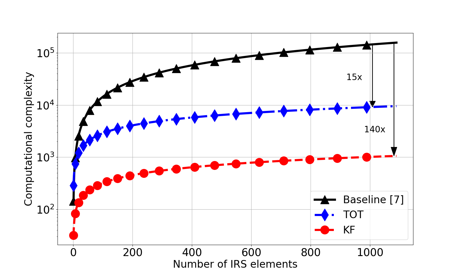
Figure 2: Computational complexity of the proposed solutions and the baseline [7] for fixed $M$ and $K$ while varying $N$.

Fig. 2 shows the computational complexity as a function of the number of IRS reflecting elements. By exploiting the Kronecker factorization structure of the channels, the KF and TOT solutions have lower slopes when compared to the baseline algorithm [7]. Although KF and TOT have small degradation in performance, they can significantly reduce the computational complexity when moderate or large numbers of IRS elements are considered and, as shown previously, depending on the scenario they can have very close performance compared to the baseline solution. For example, for $1000$ reflecting elements the baseline solution [7] is $140$ and $15$ times more complex than the proposed KF and TOT solutions, respectively.

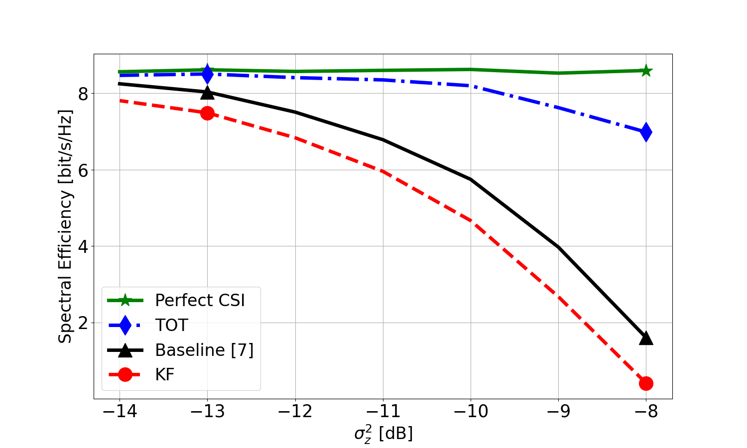
Figure 3: SE of the proposed methods and the baseline method of [7] under imperfect CSI.

Figure 3 depicts the SE of the proposed algorithms when channel estimation error is taken into account, considering $\text{SNR}=20$dB. To this end, let ${\mbox{\boldmath$\hat{F}$}}\doteq{\mbox{\boldmath$H$}}^{T}\diamond{\mbox{\boldmath$G$}}+{\mbox{\boldmath$Z$}}$ be the noisy estimate of the combined (Khatri-Rao) channel obtained after LS estimation and matched filtering with the known orthogonal pilots and optimal DFT IRS phase shift matrices (details can be found in [22]), where ${\mbox{\boldmath$Z$}}\sim\mathcal{C}\mathcal{N}(0,\sigma_{z}^{2})$ accounts for the channel estimation error. Also, define ${\mbox{\boldmath$\hat{F}$}}_{y}$ and ${\mbox{\boldmath$\hat{F}$}}_{z}$ as the noisy estimates of the $y$ and $z$ channel components of $\hat{F}$ (obtained according to [14]). The baseline method of [7] optimizes the beamforming vectors from the estimates of $H$ and $G$ obtained after a Khatri-Rao factorization step applied to the noisy estimate $\hat{F}$. The KF method relies on the decoupled estimates of ${\mbox{\boldmath$\hat{H}$}}_{y},{\mbox{\boldmath$\hat{H}$}}_{z},{\mbox{\boldmath$\hat{G}$}}_{y}$, ${\mbox{\boldmath$\hat{G}$}}_{z}$ obtained after Khatri-Rao and Kronecker factorization steps, while the TOT method operates directly on the estimates ${\mbox{\boldmath$\hat{F}$}}_{y}$ and ${\mbox{\boldmath$\hat{F}$}}_{z}$, avoiding the Khatri-Rao factorization step. The perfect CSI curve corresponds to the baseline method [7] assuming perfect CSI knowledge. As shown in Fig. 3, for higher values of $\sigma_{z}^{2}$ TOT outperforms the baseline and the KF methods due to the processing required to obtain ${\mbox{\boldmath$\hat{F}$}}_{y}$ and ${\mbox{\boldmath$\hat{F}$}}_{z}$ which rejects part of the noise. The KF has the worst performance due to the scaling ambiguities in the Khatri-Rao factorization step that propagates to the subsequent stage where the horizontal and vertical channel matrices are estimated. Hence, although TOT is more computationally complex than KF, under moderate channel estimation error, it has a better SE performance. For example, assuming $\sigma_{z}^{2}=-8$dB the TOT, baseline, and KF solutions present a SE gap of $1.6$, $7$, and $8.2$ bits/s/Hz compared to the perfect CSI curve. These results show the involved tradeoffs between complexity and performance under imperfect CSI.

V Conclusion

We proposed two low-complexity joint active and passive beamforming designs for IRS-assisted MIMO systems. Our methods exploit the geometrical channel structure to split the involved optimization problems into vertical and horizontal domains. The proposed KF and TOT algorithms significantly reduce the computational complexity with negligible SE degradation compared to the reference method under perfect CSI, while the TOT method provides the best SE performance when channel estimation noise is taken into account in the proposed optimization due to more efficient noise rejection.

References

- [1] E. Basar, M. Di Renzo, J. De Rosny, M. Debbah, M. Alouini, and R. Zhang, “Wireless Communications Through Reconfigurable Intelligent Surfaces,” IEEE Access, vol. 7, pp. 116 753–116 773, 2019.
- [2] S. Gong, X. Lu, D. T. Hoang, D. Niyato, L. Shu, D. I. Kim, and Y.-C. Liang, “Toward smart wireless communications via intelligent reflecting surfaces: A contemporary survey,” IEEE Communications Surveys & Tutorials, vol. 22, no. 4, pp. 2283–2314, June 2020.
- [3] N. A. Abbasi, J. L. Gomez, R. Kondaveti, S. M. Shaikbepari, S. Rao, S. Abu-Surra, G. Xu, J. Zhang, and A. F. Molisch, “Thz band channel measurements and statistical modeling for urban D2D environments,” IEEE Trans. Wireless Commun., vol. 22, no. 3, pp. 1466–1479, Mar 2023.
- [4] Q. Wu and R. Zhang, “Intelligent reflecting surface enhanced wireless network: Joint active and passive beamforming design,” in Proc. IEEE Globecom, Dec. 2018, pp. 1–6.
- [5] H. Song, M. Zhang, J. Gao, and C. Zhong, “Unsupervised learning-based joint active and passive beamforming design for reconfigurable intelligent surfaces aided wireless networks,” IEEE Commun. Lett., vol. 25, no. 3, pp. 892–896, Mar. 2021.
- [6] H. Ur Rehman, F. Bellili, A. Mezghani, and E. Hossain, “Joint active and passive beamforming design for IRS-assisted multi-user MIMO systems: A vamp-based approach,” IEEE Trans. Commun., vol. 69, no. 10, pp. 6734–6749, Oct 2021.
- [7] A. Zappone, M. Di Renzo, F. Shams, X. Qian, and M. Debbah, “Overhead-aware design of reconfigurable intelligent surfaces in smart radio environments,” IEEE Trans. Wireless Commun., vol. 20, no. 1, pp. 126–141, Jan. 2021.
- [8] W. Zhou, J. Xia, C. Li, L. Fan, and A. Nallanathan, “Joint precoder, reflection coefficients, and equalizer design for IRS-assisted MIMO systems,” IEEE Trans. Commun., vol. 70, no. 6, pp. 4146–4161, June 2022.
- [9] X. Zhao, K. Xu, S. Ma, S. Gong, G. Yang, and C. Xing, “Joint transceiver optimization for IRS-aided MIMO communications,” IEEE Trans. Commun., vol. 70, no. 5, pp. 3467–3482, May 2022.
- [10] E. E. Bahingayi and K. Lee, “Low-complexity beamforming algorithms for IRS-aided single-user massive MIMO mmwave systems,” IEEE Trans. Wireless Commun., vol. 21, no. 11, pp. 9200–9211, Nov 2022.
- [11] G. T. de Araújo, A. L. F. de Almeida, and R. Boyer, “Channel estimation for intelligent reflecting surface assisted MIMO systems: A tensor modeling approach,” IEEE JSTSP, vol. 15, no. 3, pp. 789–802, April 2021.
- [12] G. T. de Araújo, P. R. B. Gomes, A. L. F. de Almeida, G. Fodor, and B. Makki, “Semi-blind joint channel and symbol estimation in IRS-assisted multiuser MIMO networks,” IEEE Wireless Commun. Lett., vol. 11, no. 7, pp. 1553–1557, July 2022.
- [13] Y. Lin, S. Jin, M. Matthaiou, and X. You, “Tensor-based algebraic channel estimation for hybrid IRS-assisted MIMO-OFDM,” IEEE Trans. Wireless Commun., vol. 20, no. 6, pp. 3770–3784, June 2021.
- [14] Fazal-E-Asim, B. Sokal, A. L. F. de Almeida, B. Makki, and G. Fodor, “Tensor-Based High-Resolution Channel Estimation for RIS-Assisted Communications,” arXiv e-prints, p. arXiv:2304.05576, Apr. 2023.
- [15] Fazal-E-Asim, A. L. F. de Almeida, B. Sokal, B. Makki, and G. Fodor, “Two-dimensional channel parameter estimation for IRS-assisted networks,” 2023. [Online]. Available: http://arxiv.org/abs/2305.04393
- [16] B. Sokal, P. R. B. Gomes, A. L. F. de Almeida, B. Makki, and G. Fodor, “IRS phase-shift feedback overhead-aware model based on rank-one tensor approximation,” in Proc IEEE Globecom, Dec 2022, pp. 3911–3916.
- [17] B. Sokal, P. R. B. Gomes, A. L. F. de Almeida, B. Makki, and G. Fodor, “Reducing the control overhead of intelligent reconfigurable surfaces via a tensor-based low-rank factorization approach,” 2022.
- [18] Fazal-E-Asim, F. Antreich, C. C. Cavalcante, A. L. F. de Almeida, and J. A. Nossek, “Two-dimensional channel parameter estimation for millimeter-wave systems using butler matrices,” IEEE Trans. Wireless Commun., vol. 20, no. 4, pp. 2670–2684, April 2021.
- [19] Z. Wang, W. Liu, C. Qian, S. Chen, and L. Hanzo, “Two-dimensional precoding for 3-d massive mimo,” IEEE Transactions on Vehicular Technology, vol. 66, no. 6, pp. 5485–5490, Jun. 2017.
- [20] T. G. Kolda and B. W. Bader, “Tensor decompositions and applications,” SIAM Review, vol. 51, no. 3, pp. 455–500, 2009.
- [21] N. Kishore Kumar and J. Shneider, “Literature survey on low rank approximation of matrices,” arXiv, p. arXiv:1606.06511, Jun. 2016.
- [22] T. L. Jensen and E. De Carvalho, “An optimal channel estimation scheme for intelligent reflecting surfaces based on a minimum variance unbiased estimator,” in Proc. ICASSP 2020, 2020, pp. 5000–5004.