Topological edge state transfer via topological adiabatic passage

Abstract

The study of quantum state transfer has led to a variety of research efforts utilizing quantum simulators. By exploiting the tunability of the qubit frequency and qubit-qubit coupling, a superconducting qubit chain can simulate various topological band models. In our study, we demonstrate that a spin-up state can be transported along a topological qubit chain by modulating the coupling strengths and the qubit frequencies. We show that the Hilbert space of the qubit chain can be restricted to the subspace of two edge states in this process, while the Hamiltonian degenerates into a two-state Landau-Zener (LZ) model. Furthermore, we prove that the state transfer process in this topological qubit chain is equivalent to the topological adiabatic passage of the LZ model. With this analysis, we generalize the state transfer approach from single-qubit Fock states to two-qubit Bell states.

I Introduction

The discovery of topological insulators Hasan and Kane (2010) triggered extensive studies in topological phases of matter. Topological insulators, topological superconductors, and topological semimetals are just a few examples. It is well known that the topological power stems from its global geometric properties characterized by topological invariants. The topological protections can result in many potential applications, for example, topological quantum computation Stern and Lindner (2013), in which the non-Abelian states of matter are used to encode and manipulate quantum information in a nonlocal manner. These nonlocal global states are topologically protected, and are more robust against the decoherence of qubit states or local impurities of quantum computational devices.

Topological phenomena were first demonstrated in crystals and other condensed matter systems. Recently, the study for topological physics has been applied to photonic systems, ultracold atoms, and ultracold gases in optical lattices Lu et al. (2014); Chien et al. (2015); Goldman et al. (2016). These systems enhance the possibility to create and probe new topological phases. Furthermore, inspired by quantum computing, in which the qubits and their couplings can be controlled or tuned, topological physics is studied via quantum computational devices. The reason is twofold. First, some exotic topological states, which are not easy to find in natural systems, may be created and probed by artificially designing and fabricating on-demand quantum computational devices. Second, some topological states, which are experimentally difficult to create in natural systems, may be simulated via quantum simulators Georgescu et al. (2014).

The simplest model exhibiting topological characters is the Su-Schrieffer-Heeger (SSH) model Su et al. (1979, 1980); Heeger et al. (1988); Asbóth et al. (2016). It has been extensively studied by theorists Takayama et al. (1980); Jackiw and Rebbi (1976); Ruostekoski et al. (2002); Li et al. (2014) and attracted different experimental platforms (e.g., in Refs. Poli et al. (2015); Kitagawa et al. (2012); Cardano et al. (2017); Atala et al. (2013); Meier et al. (2016); Lohse et al. (2015); Nakajima et al. (2016)). For example, in cold atoms, the topological invariant of the one dimensional band, also known as the Zak phase Zak (1989), was measured Atala et al. (2013). Because of the bulk-edge correspondence, the band invariant is associated with the existence of edge states. The edge signal is not easy to resolve from the bulk in the real space lattice of cold atoms. Recently in the momentum space of cold atoms, the dynamics of edge states was probed Meier et al. (2016). The quantized transport of particles, known as the Thouless pump Thouless (1983), was also demonstrated in cold atoms by modulating the on-site potential and coupling strength of the SSH model Lohse et al. (2015); Nakajima et al. (2016).

Recently, topological physics is explored through superconducting quantum circuits (or superconducting artificial atoms) You and Nori (2011); Devoret and Schoelkopf (2013); Gu et al. (2017). Unlike natural atoms, these circuits can be fabricated with well-tailored characteristic frequencies and other parameters. The exquisite control of superconducting quantum circuits makes it possible to simulate topological band models on a single superconducting qubit. This is achieved by mapping the bulk momentum space of a topological band model, onto the parameter space of a spin in an external magnetic field Gritsev and Polkovnikov (2012). The Berry phase was first measured in a single superconducting qubit Leek et al. (2007); Berger et al. (2012, 2013); Schroer et al. (2014); Zhang et al. (2017). Via Berry phase, topological invariants characterizing the band properties were also measured Roushan et al. (2014); Flurin et al. (2017); Ramasesh et al. (2017). The space-time inversion symmetric topological semimetal Tan et al. (2017) and topological Maxwell metal bands Tan et al. (2018) were also simulated in a single superconducting qubit circuit. Experimental efforts are now directed to large scale of superconducting qubits. As an initial step towards realizing fractional quantum Hall effect, anyonic fractional statistical behavior is emulated in supercondcuting circuits with four qubits coupled via a quantized microwave field Zhong et al. (2016). Also, directional transport of photons was observed on a unit cell formed by three superconducting qubits Roushan et al. (2016). In this design, qubits play the role of the lattice sites, whereas the synthetic topological materials are made of photons. There are various interesting theoretical proposals to study topological physics based on superconducting circuits Koch et al. (2010); Nunnenkamp et al. (2011); Mei et al. (2015, 2016); Yang et al. (2016); Tangpanitanon et al. (2016); Sameti et al. (2017); Engelhardt et al. (2017).

Here, rather than using microwave photons coupled by superconducting qubits, we propose to simulate topological physics with a chain of coupled superconducting qubits. As a simulator of spin physics, the coupled superconducting qubits are widely studied Levitov et al. (2001); Tian (2010); Johnson et al. (2011); Viehmann et al. (2013a, b). For instance, quantum annealing was demonstrated experimentally on an Ising spin chain comprised of eight superconducting flux qubits Johnson et al. (2011). Due to the improved controllability and fabrication technique of superconducting circuits, it becomes accessible to fabricate tens of qubits with various types of couplings. The qubit frequency and qubit-qubit coupling strengths can all be tuned in situ, making the whole superconducting qubit chain versatile enough to simulate topological models Asbóth et al. (2016); Harper (1955); Aubry and André (1980). Inspired by the studies in other systems (e.g., In Refs. Poli et al. (2015); Kitagawa et al. (2012); Cardano et al. (2017); Atala et al. (2013); Meier et al. (2016); Lohse et al. (2015); Nakajima et al. (2016)), we here study topological edge states and pumping by constructing the SSH model and Rice-Mele model Heeger et al. (1988); Asbóth et al. (2016) using gap-tunable flux qubit circuits Paauw et al. (2009); Paauw (2009); Schwarz et al. (2013); Zhu et al. (2010).

The paper is organized as follows. In Section II, we briefly introduce the topological qubit chain constructed of gap-tunable flux qubits. This spin chain model can be mapped to SSH model or Rice-Mele model when restricted to single excitation subspace. In Section III, we show that the single-qubit edge state can be transported from one end of the chain to the other end by adiabatic pumping. We theoretically analyze this pumping process and propose one optimized pumping protocol. In  Section IV, we generalize the state pumping protocol to two-qubit state transfer with a trimer Rice-mele model. In Section V, we summary our results and further discuss possible demonstration on topological physics using superconducting qubit circuits. For the completeness of the paper, we also give a detailed superconducting circuit analysis for the spin chain in the appendix.

II Topological qubit chain with superconducting qubits

As schematically shown in Fig. 1(a), we study a superconducting quantum circuit, in which $2N$ identical superconducting qubits are coupled to form a chain with alternating coupling strengths. That is, the coupling strength between the qubit (marked in green) on the odd sites and its right neighbor (marked in orange) is $a$, while the coupling strength between the qubit (marked in orange) on the even sites is coupled to its right neighbor (marked in green) with an amplitude of $b$. It is well known that the coupling constants $a$ and $b$ between qubits can be designed to be tunable in superconducting qubit circuits by using, e.g.,  additional coupler, variable qubit frequency, detuning between qubits, or frequency matching Liu et al. (2006, 2007); Grajcar et al. (2006); Rigetti et al. (2005); Bertet et al. (2006); Niskanen et al. (2006); Hime et al. (2006); Niskanen et al. (2007); Harris et al. (2007); van der Ploeg et al. (2007); Allman et al. (2010); Bialczak et al. (2011).

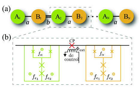
Figure 1: (a) Schematic diagram of a one-dimensional topological qubit chain. Each unit cell hosts two qubits, labeled as $A_{n}$ and $B_{n}$ separately. The coupling strengths between $A_{n}$ and $B_{n}$ are staggered, denoted as $a$ and $b$. Each qubit can also be labeled by one increasing numerical index $j$ from left to right. (b) Realization of the qubit chain with gap-tunable flux qubits. Each qubit contains two basic superconducting circuit elements, i.e., the josephson junction and the inductance. Two adjacent qubits are coupled through a tunable coupler (CP). The qubit-qubit coupling can be tuned via an external magnetic flux $\Phi_{\mathrm{ext}}$ with a dc control. The signs $\bigodot$ denote that the magnetic fluxes are directed outside. We use reduced magnetic fluxes $f_{\alpha}=\Phi_{\alpha}/\Phi_{0}$, $f_{\epsilon_{1}}=\Phi_{1}/\Phi_{0}$, and $f_{\epsilon_{2}}=\Phi_{2}/\Phi_{0}$. Here $\Phi_{\alpha}$, $\Phi_{1}$ and $\Phi_{2}$ are the magnetic fluxes through the three small loops of the qubit. $\Phi_{0}$ is the flux quanta. The frequency of the gap-tunable flux qubit can be tuned via the magnetic flux through the $\alpha$-loop or main loop, thus both the qubit frequencies and the couplings in the qubit chain are tunable.

In principle, the coupled qubit chain can be constructed by any type of superconducting qubits, e.g., flux qubits Orlando et al. (1999); Liu et al. (2005a), transmon Koch et al. (2007), xmon Barends et al. (2013) and gmon Chen et al. (2014); Geller et al. (2015). Compared with the qubits Koch et al. (2007); Barends et al. (2013); Chen et al. (2014); Geller et al. (2015), the gap-tunable flux qubit circuit Paauw et al. (2009); Paauw (2009); Schwarz et al. (2013); Zhu et al. (2010) has negligibly small population leakage from the first excited state to other upper states when the two lowest energy levels are operated as the qubit near the optimal point. Also the frequency of the gap-tunable flux qubit can be tuned via the magnetic flux through the $\alpha$-loop or main loop. Moreover, the gap-tunable flux qubit has better coherent time. Thus, for concreteness of the discussions and as an example, we first assume that each qubit in the chain is implemented by a gap-tunable flux qubit circuit Paauw et al. (2009); Fedorov et al. (2010); Schwarz et al. (2013), as schematically shown in Fig. 1(b) and is further explained in Appendix A. Through the detailed study below for the chain of the gap-tunable flux qubit circuit, we will give the comparative summary for the chain formed by other types of superconducting qubits in the discussions.

The qubit chain consists of $N$ unit cells, and each unit cell contains two sublattices labeled as $A_{n}$ and $B_{n}$ with $n=1,2,\cdots,N$. The couplings between adjacent qubits are staggered, denoted as $a$ and $b$. Here we relabel each qubit in the chain by one increasing index $j$ from $A_{1}$ to $B_{N}$, then the Hamiltonian of such a qubit chain can be written as ($\hbar=1$)

$$H = \sum_{j=1}^{2N}\frac{\omega_{j}}{2}\sigma_{j}^{z}+\sum\limits_{{j\in\mathrm{odd}}}^{2N}a(\sigma_{j}^{+}\sigma_{j+1}^{-}+{\text{H}.c.})$$ (1)

$$+ \sum\limits_{{j\in\mathrm{even}}}^{2N}b(\sigma_{j}^{+}\sigma_{j+1}^{-}+{\text{H}.c.}),$$

with $\omega_{j}$ denoting the frequency of the qubit. $\sigma_{j}^{+}$ and $\sigma_{j}^{-}$ are the creation and annihilation operators of the $j$th qubit.

The upper Hamiltonian can degenerate into the Rice-Mele model or SSH model when restricted to the single-excitation subspace of the qubit chain. In most studies, the qubit operator is mapped onto the non-interacting fermions through Jordan-Wigner transformation Fradkin (2013). However, here we find that the total spin excitation $\sum_{j=1}^{2N}\sigma_{j}^{z}$ commutes with Hamiltonian $H$ in Eq. (1). Thus the number of total excitations of the qubit chain is conserved. In the following analysis, instead of resorting to the nonlocal Jordan-Wigner transformation, we restrict our study in the single-excitation subspace. That is, only one qubit is excited in the qubit chain. This can be done in superconducting quantum circuits due to the strong anharmonicy of the flux qubit. We define the basis in single-excitation subspace as

$$|e_{j}\rangle=|0,...,1_{j},0...\rangle,$$ (2)

where the $j$th superconducting qubit is assumed in the spin-up state $|1_{j}\rangle$, while the other qubits are in the spin-down states $|0\rangle$. Thus in the subspace with only one excitation, the Hamiltonian $H$ in Eq. (1) has the tridiagonal form as

$$H_{S}=\begin{bmatrix}\omega_{1}&a&&&&\\ a&\omega_{2}&b&&&\\ &b&\omega_{3}&a&&\\ &&\ddots&\ddots&\ddots&\\ &&&b&\omega_{N-1}&a\\ &&&&a&\omega_{N}\end{bmatrix}.$$ (3)

Here, the subscript $S$ denotes the single-excitation. If the qubits on odd(even) sites are identical, then the Hamiltonian $H_{S}$ can be reduced to the Rice-Mele model as

$$H_{\text{RM}} = \sum_{n}\left(\omega_{1}A_{n}^{\dagger}A_{n}+\omega_{2}B_{n}^{\dagger}B_{n}\right)$$ (4)

$$+ \sum_{n}\left(aA_{n}^{\dagger}B_{n}+bB_{n}^{\dagger}A_{n+1}+\text{H.c.}\right),$$

where $A_{n}$ and $B_{n}$ are the single-excitation annihilation operators of each qubit in the $n$th unit cell, which can be expanded as $A_{n}=|\textrm{\O}\rangle\langle\textrm{$e_{2n-1}$}|$ and $B_{n}=|\textrm{\O}\rangle\langle\textrm{$e_{2n}$}|$. Here $|\textrm{\O}\rangle$ denotes that all qubits in the chain are in the ground state, i.e., $|\textrm{\O}\rangle=|0,\ldots,0\rangle$.

Furthermore, if all the qubits are identical, that is, $\omega_{j}=\omega$ with $j=1,\cdots,2N$, then the Hamiltonian in Eq. (4) is equivalent to the SSH model Asbóth et al. (2016). After shifting the zero-energy point to $\omega$, this single-excitation Hamiltonian is given by

$$H_{\mathrm{SSH}}=\sum_{n}\left(aA_{n}^{\dagger}B_{n}+bB_{n}^{\dagger}A_{n+1}+\mathrm{H.c.}\right).$$ (5)

The SSH model describes a chain of dimers, each hosting two sites A and B. The hopping strength within the unit cell is $a$, the intercell hopping amplitude is $b$. In our qubit chain as schematically shown in Fig. 1, the odd (even) number of the qubits in Eq. (1) corresponds to the A (B) particles in Eq. (5). For this standard SSH model, the topological phases are characterized by winding numbers Asbóth et al. (2016). According to the bulk-edge correspondence Hasan and Kane (2010), two topological edge states are supported when the qubit chain is in the topological nontrivial phase. In Appendix C, we study the quench dynamics of the SSH chain when the first qubit is initially prepared in the spin-up state. As we can see, in the topological nontrivial phase the existence of edge states reveals itself as a soliton localized at the very end of the chain, while in the topological trivial phase the excitation at the first qubit will quickly diffuse into the bulk.

The edge states are topologically protected and robust against disorder, thus it is quite straightforward to utilize these edge state for quantum state transfer. To precisely control the whole process, we need another degree of freedom as the parameter, i.e., the on-site potentials of the qubits. Below we show how to transfer quantum states in the superconducting qubit chain mapped onto the Rice-mele model.

III Topological analysis of edge state transfer

For one topological chain, once an excitation is injected at the edge, it will stay as a soliton. Therefore, such property of preserving quantum states gives topological matter great potential to store quantum information, which is a basic task of quantum information processing. Another basic task of quantum information processing is robust quantum state transfer. Fortunately, with the topological property of edge states in the topological qubit chain, it is possible to transfer the soliton edge state from the left end to the right end of the chain by adiabatic pumping.

Hereafter, we will firstly propose an straightforward proposal of transferring an edge state in the qubit chain. Then, a topology analysis will be given for such quantum state transfer process. Finally, based on the topology analysis, we will give an optimized protocol with better accuracy and robustness.

III.1 Pumping of an edge state

If the on-site potentials of the Hamiltonian in Eq. (1) are staggered as $u$ and $-u$, the qubit chain can be mapped to the Rice-Mele model. The pumping can be realized if the staggered potentials and the coupling strengths in the Hamiltonian can be modulated. Such time modulations for qubit frequencies and coupling strengths can be realized in superconducting qubit circuits as discussed in Appendix B.

If we only consider the single-excitation states, as discussed in Section II, the time-dependent Hamiltonian in Eq. (B.2.2) with qubit frequency modulations can be reduced to the Hamiltonian of the Rice-Mele model Rice and Mele (1982); Asbóth et al. (2016) as

$$H_{\mathrm{RM}} = \sum_{n}\left[a(t)A_{n}^{\dagger}B_{n}+b(t)A_{n}^{\dagger}B_{n-1}+\mathrm{H.c.}\right]$$ (6)

$$+ u(t)\sum_{n}(A_{n}^{\dagger}A_{n}-B_{n}^{\dagger}B_{n}),$$

where $A_{n}^{\dagger}$ ($B_{n}^{\dagger}$) is the particle creation operator on the site A (B) in the $n$th cell, $a(t)$ and $b(t)$ are the time dependent coupling strengths, $u(t)$ is the staggered potential. This Rice-Mele Hamiltonian can be continuously deformed along the time-dependent pump sequences given by $u(t)$, $a(t)$ and $b(t)$. In superconducting quantum circuits, this can be done by varying the magnetic fluxes through the couplers and the $\alpha$ loops of the supercoducting qubits.

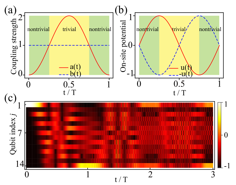
Figure 2: (a) The coupling strengths $a$ and $b$ versus time $t$. (b) The on-site potentials $u$ and $-u$ versus time $t$. (c) Time evolution of the particle distributions $\langle\sigma_{j}^{z}\rangle$ for the qubit chain of $2N=14$ qubits. The time-dependent pump sequence is defined in Eq. (III.1), with $T=100$. The color from dark-red to bright-yellow represents the particle distribution $\langle\sigma_{j}^{z}\rangle$ varying from $-1$ to $1$.

For example, as shown in Fig. 2, we can demonstrate the topological pumping by simply choosing the coupling strengths $a(t)$ and $b(t)$ as well as the on-site potential $u(t)$ as

$$a(t) = 1-\cos\left(\frac{2\pi t}{T}\right),$$

$$b(t) = 1,$$

$$u(t) = \sin\left(\frac{2\pi t}{T}\right).$$ (7)

where $T$ is the variation period of these parameters. Figures 2(a) and (b) show the time-dependent coupling strengths and on-site potentials versus time $t$ during one period. The numerical simulation of the dynamical evolution of the qubit chain, as shown in Fig. 2(c), is solved using ordinary differential equation solver based on backward differentiation (BDF) formulas Wanner and Hairer (1996). The result shows that the soliton edge state can indeed be transferred from one end of the chain to the other end within one pumping cycle. To ensure the adiabatic limit, we set $T=100$. The chain is initialized in the all spin-down state. To prepare the left edge state, the first qubit is flipped by a $\pi$ pulse of the applied magnetic flux through the main loop of the qubit. However, this pumping process somehow can’t last more than one circle.

The instantaneous spectrum of the Hamiltonian in Eq. (6) is plotted as a function of $t$ in Fig. 3(a). The black-solid lines represent the bulk states and the color-dashed lines represent the edge states. According to the quantum adiabatic theorem (berry’s article), if the adiabatic approximation holds during the pumping circles, the system will stay in the same eigenstate as the prepared initial state. With the increasing of the on-site potential, two degenerate edge states separate from each other and develop into two branches. As shown in Fig. 3(b), the state on point b of the upper branch is mostly located on the left end of the chain. Therefore, if the initial state is prepared as the left edge state, it will adiabatically evolve following the upper branch as shown in the red-dashed line in Fig. 3(a).

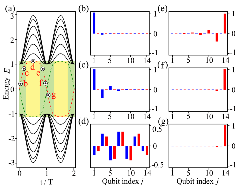
Figure 3: (a) Instantaneous spectrum of the Hamiltonian in Eq. (6) with the pumping sequence defined in Eq. (III.1). The chain consists of $2N=14$ qubits. When $t>0$, the on-site potential will relieve the degeneracy of two edge states and break the degenerate energies into two branches, as shown in the red- and green-dashed lines. Five particular states on the upper branch are chosen as b, c, d, e, f, and g. The corresponding wave functions are shown in (b) to (g).

The wave functions of six particular points on the upper branch are plotted in Fig. 3(b) to (g). For the first pumping cycle, the result shown in Fig. 2(c) is consistent with the adiabatic limit in Fig. 3. The soliton first diffuses as the left edge state with vanishing amplitudes on the even sites. Then it is pushed into the bulk occupying both even and odd sites. After that, it reappears as the right edge state with vanishing amplitudes on the odd qubits. At the end of the first pumping cycle, as shown in Fig. 3(f), the right edge state refocuses on the right end qubit. The soliton edge state is already transferred from the left end to the right end before the crossing point. As shown in Fig. 3(g), the eigenstate in point g is the same in point f. Indeed, after this crossing point, the evolving route follows the red-dashed line from point f to point g, which is also verified in Fig. 2(c). Apparently, the evolution of the state around the level crossing does not follow the traditional adiabatic theorem, which will be discussed later in Section III.2.

Through the wave functions at points b to f in Fig. 3, we have shown how a left edge state is adiabatically pumped to the right during a pumping cycle. It is seen that the state occupies the left edge and right edge equally in point d. We denote this to be the transition point. Combining Fig. 2 and Fig. 3, we can summarize two principles to achieve the edge state transfer. The first one is that, as shown in Fig. 2(b), the on-site potential $u(t)$ must change sign at the transition point, i.e., $t=T/2$. The second one is that, to insure the adiabaticity, the energy gap must be opened between two branches during the state transfer process, i.e., the coupling strengths can’t be zero around the transition point, as shown in Fig. 2(a). Based on these two principles, we can easily redesign some other time-dependent pump sequences to achieve QST.

In our pump result, only the edge mode is occupied initially, while the lower band is empty. However, in the cold atom experiments Lohse et al. (2015); Nakajima et al. (2016), all the lower band is filled with the atoms, while the upper band is empty. During a pumping cycle, each atom in the valence band is moved to the right by a single lattice constant. Or equivalently, the number of pumped particles through the cross section is one. This is determined by the Chern number of the associated band Asbóth et al. (2016). By promoting the periodic time $t$ to the wave-number, the adiabatic pump sequence in one dimension is equivalent to two-dimensional insulators.

III.2 Topology of the pumping process

When the on-site potentials $u$ are equal to $0$, the former Rice-Mele model in Eq. (6) is reduced to the SSH model. As discussed in Section. C, for a standard SSH model in the nontrivial topological phase, i.e., $|a|<|b|$, two existing topological edge states are denoted as $|L\rangle$ and $|R\rangle$. While the coupling coefficients $a$ and $b$ are positive real numbers, two edge states can be expressed as

$$|L\rangle=\Xi\sum_{n}\lambda^{n-1}|e_{2n-1}\rangle$$ (8)

and

$$|R\rangle=\Xi\sum_{n}\lambda^{L-n}|e_{2n}\rangle$$ (9)

where $\Xi=\sqrt{\left(1-\lambda^{2}\right)/\left(1-\lambda^{2N}\right)}$ is the normalization factor and $\lambda=-a/b$ is the ratio of the coupling coefficients. In the nontrivial topological phase, the two edge states $|L\rangle$ and $|R\rangle$ hybridize under the Hamiltonian $H$ to an exponentially small amount, meanwhile, the couplings between the edge states and the bulk states are much exponentially smaller. With a good approximation using adiabatic elimination of the other bulk states Asbóth et al. (2016), we can investigate the state transfer process in the subspace of $\{|L\rangle,|R\rangle\}$. This idea of restricting the Hilbert space of the dynamic process can also be generalized to the Rice-Mele model Longhi et al. (2019); Chen et al. (2021); Shen et al. (2021). As for the our system shown in Eq. (6), the matrix elements of the effective Hamiltonian in this subspace take the following forms as

$$\langle L|H|L\rangle=-\langle R|H|R\rangle=u,$$ (10)

$$\langle L|H|R\rangle=\langle R|H|L\rangle=\Xi^{2}a\lambda^{L-1}.$$ (11)

Hence the effective Hamiltonian can be written as

$$H=\left(\begin{array}[]{cc}u&g\\ g&-u\end{array}\right),$$ (12)

where $g=\Xi^{2}a\lambda^{L-1}$ is the effective coupling strength between two edge states. Thus, we transform the complicated many-body problem into a two-state quantum dynamics.

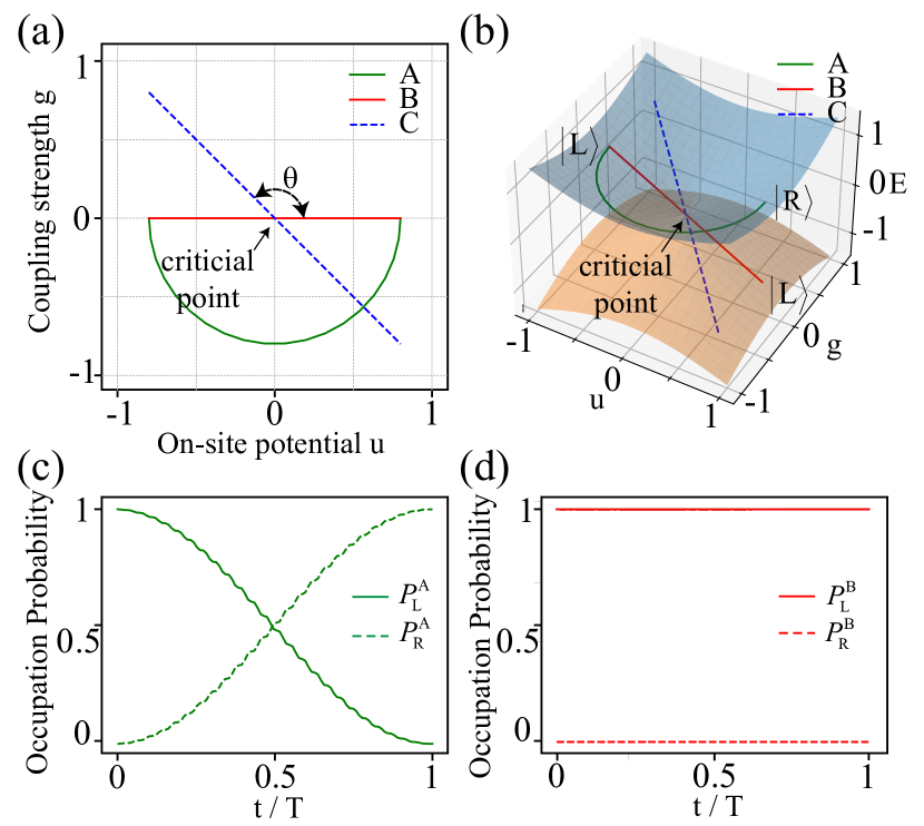
Figure 4: (a) Three paths shown in the parameter space of on-site potential $u$ and coupling strength $g$. (b) The energy spectrum of the two-level system. Different parameter paths of the same start point and end point can lead to different evolution paths. (c) Time evolution of state occupation along path A. (d) Time evolution of state occupation along path B.

For a two-state Landau-Zener (LZ) model Landau and Lifshitz (1977) shown in Eq. (12), we can characterize the adiabatic state transfer processes based on the topology of the eigenenergy surfaces Yatsenko et al. (2002). The eigenenergies of the effective Hamiltonian in Eq. (12) are

$$E_{\pm}=\pm\sqrt{u^{2}+g^{2}}.$$ (13)

The two eigenenergy surfaces can be drawn as a dirac cone shown in Fig. 4(b), and the two energy bands intersect at the critical point $u=0$ and $g=0$. There are two basic types of topological passages depending on whether the adiabatic evolution path goes through the critical point.

To illustrate the differences between these two passages, we particularly choose two paths with the same start point and end point as shown in the solid lines in Fig. 4(a). The green path A is an arc and can be described as

$$u=\alpha\cos\left(\frac{\pi t}{T}-\pi\right),g=\alpha\sin\left(\frac{\pi t}{T}-\pi\right).$$ (14)

Due to the quantum adiabatic theorem Messiah (1962); Berry (1984), if the parameters of the quantum system are changed slowly enough, it will remain in its instantaneous eigenstate. As shown in Fig. 4(b), if the initial state is prepared as $|L\rangle$ on the upper branch, the adiabatic following of the path A can induce the complete state transfer from $|L\rangle$ to $|R\rangle$. This adiabatic process is verified with numerical simulation as shown in Fig. 4(c). The red path B is a straight line and can be described as

$$u=\alpha\left(\frac{2t}{T}-1\right),g=0.$$ (15)

As shown in Fig. 4(b), the two bands merge at the critical point in the section of $g=0$, and hence the adiabatic following here should be handled more carefully. Notice that if $g=0$, the two states $|L\rangle$ and $|R\rangle$ are decoupled from each other. Therefore, as the parameter $u$ changes continuously, the system will remain in the same state. This evolution process is verified with numerical simulation as shown in Fig. 4(d).

More generally, an arbitrary straight path through the critical point can be described as

$$u=\alpha\left(\frac{2t}{T}-1\right),g=\tan\left(\theta\right)u$$ (16)

as shown in the blue-dashed line in Fig. 4(a). The Hamiltonian of this path C can be written as

$$H=\frac{u}{\cos\theta}\left(\begin{array}[]{cc}\cos\theta&\sin\theta\\ \sin\theta&-\cos\theta\end{array}\right).$$ (17)

Eigenstates of the Hamiltonian in Eq. (17) have the form

$$\left[\begin{array}[]{c}|\uparrow\rangle\\ |\downarrow\rangle\end{array}\right]=\left(\begin{array}[]{cc}\cos\frac{\theta}{2}&\sin\frac{\theta}{2}\\ \sin\frac{\theta}{2}&\cos\frac{\theta}{2}\end{array}\right)\left[\begin{array}[]{c}|L\rangle\\ |R\rangle\end{array}\right].$$ (18)

These two eigenstates are time-independent and the corresponding eigenenergies are $E=\pm u/\cos\theta$. Therefore, the Hamiltonian in the basis of $|\uparrow\rangle$ and $|\downarrow\rangle$ can be written as

$$H=\frac{u}{\cos\theta}\left(\begin{array}[]{cc}1&0\\ 0&-1\end{array}\right).$$ (19)

From this perspective, the two states $|\uparrow\rangle$ and $|\downarrow\rangle$ are decoupled from each other. If the initial state is prepared as $|\uparrow\rangle$ or $|\downarrow\rangle$, the system will remain in the same state over time. In the Fig. 4(b), we show the state on the path C initially prepared as $|\uparrow\rangle$ evolves from the upper branch to the lower branch across the critical point. Thus, the adiabatic passage around the critical point support the state transfer, while the adiabatic passage through the critical point leaves the system in the same state.

As for the state transfer proposal in Section III.1, the parameters of the effective Hamiltonian can be derived from Eqs. (III.1), (10) and (11). The path of this adiabatic passage in parametric space is shown in Fig. 5(a). The whole evolution process can be divided into three stages denoted as red-solid line, green-dashed line and blue-solid line, individually. The solid lines represent the topological nontrivial region and the dashed line represents the topological trivial region. As shown in Fig. 5(b), in the first stage, the on-site potentials rise up and the system keeps the same state, i.e., $|L\rangle\rightarrow|L\rangle$. In the second stage, the state evolves from the left edge into the bulk and then reaches to the right edge, i.e., $|L\rangle\rightarrow bulk\rightarrow|R\rangle$. In the third stage, the on-site potentials decrease to $0$ and the system maintains the same state, i.e., $|R\rangle\rightarrow|R\rangle$. Therefore, after one pumping cycle, the state is transferred from the left edge to the right edge.

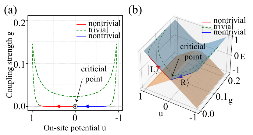
Figure 5: (a) The path of the adiabatic passage of the effective Hamiltonian in the parametric space. (b) Evolution path of the adiabatic passage in the energy spectrum.

As discussed before, the approximation of adiabatic elimination of bulk states works only in the topological nontrivial region. In the topological trivial region, the couplings between the edge states and the bulk states can not be ignored, and the dashed lines of the second stage in Fig. 5 are not the real evolution path. Nevertheless, the energy bands in the topological trivial region are separated from each other as shown in Fig. 3, and the adiabatic following is still feasible in this region. Therefore, after the first stage, the state is confirmed to evolve from the left edge into the bulk. The three-stage description of the state transfer process is still applicable.

III.3 Optimization of the pumping cycle

With the analysis above, it is easy to conclude that the inaccuracy of the pumping does not come from the crossing energy levels, but from the close energy bands in the topological trivial region. Hence we need to adjust the system parameters to get larger gaps between the adiabatic passage and other bulk states in our advanced pump protocol as compared with Fig. 3.

As shown in Fig. 3, in the first topological nontrivial region, the energy of the edge state increases with the on-site potential before the edge state joins the bulk. Thus the first clew is to decrease the amplitude of the on-site potential. Here we choose the on-site potential as $u(t)=0.25*\sin\left(2\pi t/{T}\right)$. As shown in Fig. 6(a), the maximum energy of the edge state indeed decreases in the topological nontrivial region, but the edge state still joins the bulk hereafter in the topological trivial region due to the topological phase transition. Therefore the second clew is to avoid the topological phase transition so that the edge state can be well isolated from the bulk. Here apart from the modified on-site potential $u\left(t\right)$, we further choose the coupling strength $a$ as $a(t)=0.5*\left[1-\cos\left(2\pi t/T\right)\right]$, so that the relation $a<b$ can be conserved during the whole pumping cycle and the system will stay in the topological nontrivial region. As shown in Fig. 6(b), the adiabatic passage is well isolated with other bulk states during the whole quantum state transfer process.

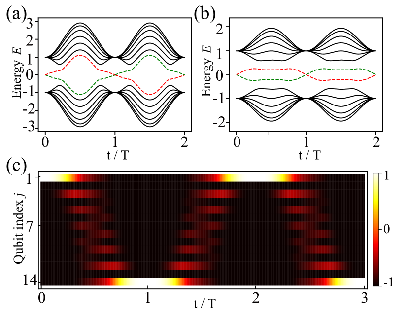
Figure 6: (a) The energy spectrum of the chain with $u(t)=0.25*\sin\left(2\pi t/{T}\right)$. (b) The energy spectrum of the chain with $u(t)=0.25*\sin\left(2\pi t/{T}\right)$ and $a(t)=0.5*\left[1-\cos\left(2\pi t/T\right)\right]$. (c) Time evolution of the particle distributions $\langle\sigma_{j}^{z}\rangle$ for the qubit chain. The color from dark-red to bright-yellow represents the particle distribution $\langle\sigma_{j}^{z}\rangle$ varying from $-1$ to $1$.

In Fig. 6(c), the numerical simulation of the qubit chain’s dynamical evolution is well resolved. With the parameters above, the initial state prepared on the first site of the chain can be perfectly transferred to the last site in a pumping cycle. This pumping process can last for many pumping cycles with high fidelity. Therefore, we can indeed optimize our pumping protocol using the topological analysis in Section III.2.

IV Two-qubit Bell state pumping in a Trimer Rice-Mele Model

Above from the perspective of the traditional adiabatic theorem, we have exhibited a more ordinary way to understand the thouless pumping in 1D Rice-Mele model. With this comprehensible explanation, we can easily generalize the state transfer protocol to a trimer Rice-Mele qubit chain.

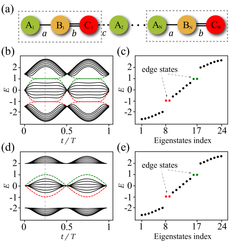
Figure 7: (a) Schematic diagram for a trimer qubit chain.The $3$ identical sites in each unit cell are denoted by green circle, orange circle and red circle. $a$ and $b$ denote the intracell coupling strengths, while $c$ denotes the intercell coupling strength. (b) The energy spectrum with respect to the intercell coupling $c(t)$ (unit cells $N=8$). The green dashed line and red dashed line represent the edge modes. (c) The eigenstates distribution on the black dashed line in (b). (d) The energy spectrum with respect to the intracell couplings. (e) The eigenstates distribution on the black dashed line in (d).

As shown in Fig. 7, the trimer Rice-Mele model is a periodic qubit chain with the unit cell of three cites. The Hamiltonian of the trimer RM model can be written as

$$H_{\text{TRM}} = \sum_{n}\left[aA_{n}^{\dagger}B_{n}+bB_{n}^{\dagger}C_{n}+cC_{n}^{\dagger}A_{n+1}+\text{H.c.}\right]$$ (20)

$$+ \sum_{n}\left[uA_{n}^{\dagger}A_{n}+vB_{n}^{\dagger}B_{n}+wC_{n}^{\dagger}C_{n}\right]$$

where $A_{n}^{\dagger}$, $B_{n}^{\dagger}$ and $C_{n}^{\dagger}$ are the particle creation operators on the sites A, B and C in the $n$th unit cell. $a$, $b$ and $c$ are the coupling strengths between each sites. $u$, $v$ and $w$ are the staggered potentials on sites A, B and C.

When the on-site potentials are chosen to be $0$, the trimer Rice-Mele model in Eq. (20) is reduced to the extended SSH3 model. As shown in Ref. Anastasiadis et al. (2022), there are generally two different cases for the topological characterization of this SSH3 model. One is the mirror symmetry case ($a=b$) and the other is the none mirror symmetry case ($a\neq b$). For the convenience of discussion, we only consider the mirror symmetry case hereafter. In this case, the Hamiltonian exhibits a band gap closing when $a=b=c$, and the edge states emerge at this gap closing point in the thermodynamic limit Anastasiadis et al. (2022).

In Fig. 7(b), we plot the energy spectrum with respect to the intercell coupling $c$, which depends on the time $t$. The coupling strengths are chosen as

$$a=b=1,c\left(t\right)=2\sin\left(\frac{2\pi t}{T}\right).$$ (21)

The edge states only exist in the region $c(t)>a$, where the SSH3 model has the nontrivial topology. We can easily notice that there are 4 edge states divided by 2 gaps. The edge states in each gap are degenerate when $c(t)\gg a$. Specifically, the eigenstates distribution at $c(t)=2$ is plotted in Fig. 7(c). The two pairs of degenerate edge states are clearly shown in red dots and blue dots.

Considering the former thouless pumping protocol, we can plot another energy spectrum with respect to the intracell couplings as shown in Fig. 7(d). The coupling strengths are chosen as

$$a\left(t\right)=b\left(t\right)=\sin\left(\frac{2\pi t}{T}\right),c=2$$ (22)

where the intracell couplings are time-dependent and the intercell coupling $c$ is constant. With the parameters above, the system remains in the topologically trivial region, so the edge states are degenerate all along. We can also clarify the degenerate edge states with the eigenstates distribution in Fig. 7(e).

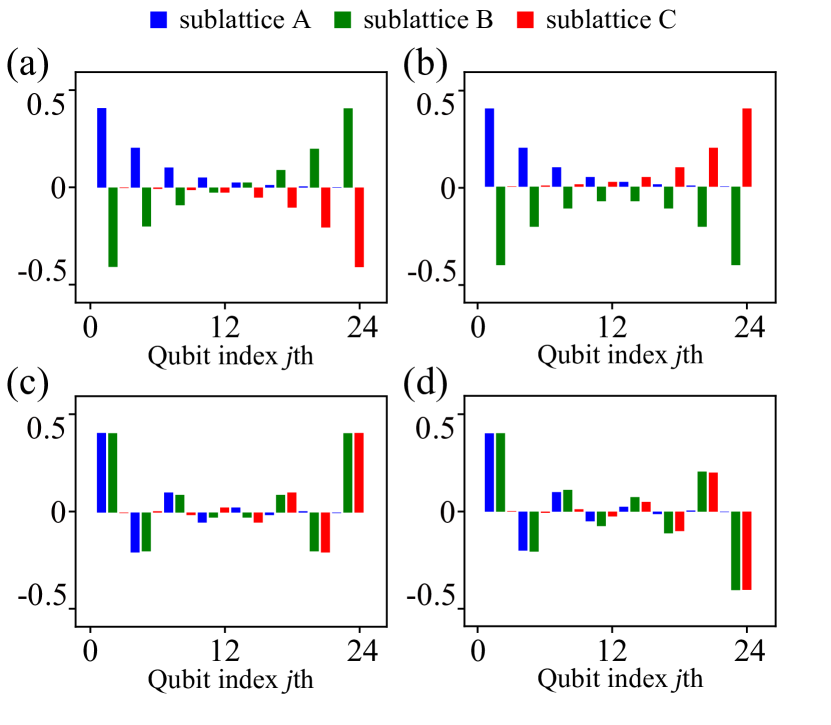
Figure 8: The wave functions of four hybridized edge states exhibited in Fig. 7(e). (a) and (b) show the hybridized edge states in the lower gap. (c) and (d) show the hybridized edge states in the upper gap.

In a finite size SSH3 model, there must be a exponentially small overlap between the left and the right edge states. Thus the wave functions of the eigenstates in the bulk band gaps must be the superpositions of the left and the right edge states. In the nontrivial topological phase, four existing edge states of the SSH3 model can be denoted as $|L_{\pm}\rangle$ and $|R_{\pm}\rangle$. The localized eigenfunctions in the lower and upper band gaps can be individually expressed as $\left(|L_{-}\rangle\pm|R_{-}\rangle\right)/\sqrt{2}$ and $\left(|L_{+}\rangle\pm|R_{+}\rangle\right)/\sqrt{2}$. In Fig. 8, we plot the wave functions of the four hybridized edge states. The pattern of these hybridized wave functions is just the same as the original SSH model in Section C. Therefore, we can easily derive the forms of the four edge states as

$$|L_{\pm}\rangle=\Xi\sum_{n}\left(\mp\lambda\right)^{n-1}\left(\frac{|e_{3n-2}\rangle\pm|e_{3n-1}\rangle}{\sqrt{2}}\right)$$ (23)

and

$$|R_{\pm}\rangle=\Xi\sum_{n}\left(\mp\lambda\right)^{L-n}\left(\frac{|e_{3n-1}\rangle\pm|e_{3n}\rangle}{\sqrt{2}}\right)$$ (24)

where $\Xi=\sqrt{\left(1-\lambda^{2}\right)/\left(1-\lambda^{2N}\right)}$ is the normalization factor and $\lambda=a/c$ is the ratio of the coupling coefficients.

IV.1 The state pumping process in the subspace of edge states

The whole analysis of the trimer Rice-Mele model above is in the mirror symmetric case, i.e. $a=b$. Therefore the Hamiltonian in Eq. (20) can be rewritten as

$$H_{\text{TRM}} =\sum_{n}\left[a\left(A_{n}^{\dagger}B_{n}+B_{n}^{\dagger}C_{n}\right)+cC_{n}^{\dagger}A_{n+1}+\text{H.c.}\right]$$

$$+\sum_{n}\left[uA_{n}^{\dagger}A_{n}+vB_{n}^{\dagger}B_{n}+wC_{n}^{\dagger}C_{n}\right].$$ (25)

Following the lead of the former analysis in Section III.2, we can firstly rewrite the system Hamiltonian in the subspace of $\{|L_{\pm}\rangle,|R_{\pm}\rangle\}$. As shown in Fig. 7, when $v\neq 0$, the upper edge states are well isolated from the lower edge states, so we can further divide this subspace into two individual subspaces $\{|L_{+}\rangle,|R_{+}\rangle\}$ and $\{|L_{-}\rangle,|R_{-}\rangle\}$. As for our trimer Rice-Mele system shown in Eq. (20), the matrix elements of the effective Hamiltonian in the edge state subspace take the following forms as

$$\langle L_{+}|H|L_{+}\rangle=a+\frac{u+v}{2},\langle R_{+}|H|R_{+}\rangle=a+\frac{v+w}{2}$$ (26)

$$\langle L_{+}|H|R_{+}\rangle=\langle R_{+}|H|L_{+}\rangle=\frac{L\left(a+v\right)+a}{2}\Xi^{2}\left(-\lambda\right)^{L-1}$$ (27)

$$\langle L_{-}|H|L_{-}\rangle=-a+\frac{u+v}{2},\langle R_{-}|H|R_{-}\rangle=-a+\frac{v+w}{2}$$ (28)

$$\langle L_{-}|H|R_{-}\rangle=\langle R_{-}|H|L_{-}\rangle=\frac{L\left(a+v\right)+a}{2}\Xi^{2}\lambda^{L-1}$$ (29)

Thus the effective Hamiltonian in the edge state subspace can be described as

$$H=\left(\begin{array}[]{cc}H_{+}\\ &H_{-}\end{array}\right),$$ (30)

where $H_{+}$ and $H_{-}$ represent the Hamiltonian in the upper subspace $\{|L_{+}\rangle,|R_{+}\rangle\}$ and the lower subspace $\{|L_{-}\rangle,|R_{-}\rangle\}$, respectively. Hence $H_{+}$ and $H_{-}$ are given by

$$H_{+}=\left(\begin{array}[]{cc}\frac{u}{2}&g_{+}\\ g_{+}&\frac{w}{2}\end{array}\right)+\left(a+\frac{v}{2}\right)I$$ (31)

and

$$H_{-}=\left(\begin{array}[]{cc}\frac{u}{2}&g_{-}\\ g_{-}&\frac{w}{2}\end{array}\right)-\left(a-\frac{v}{2}\right)I,$$ (32)

where $I$ is identity matrix, $g_{+}$ and $g_{-}$ are the coupling strengths between the edge states, given by

$$g_{\pm}=\frac{L\left(a+v\right)+a}{2}\Xi^{2}\left(\mp\lambda\right)^{L-1}$$ (33)

The effective Hamiltonians $H_{+}$ and $H_{-}$ have the same form as in Eq. (12). Thus we can achieve the quantum state transfer via the same adiabatic passages.

IV.2 Two-qubit Bell state transfer via the trimer Rice-Mele model

As discussed before, the adiabatic quantum state transfer process needs to begin in the topological nontrivial region, i.e. $a\ll c$. In the first stage, the on-site potential of the left edge should be much larger than that of the right edge, i.e. $u\gg w$. With the evolution of the system, the on-site potentials $u$ and $w$ of the left and right edge states exchange their values slowly. At some point, there will be a moment that these two potentials reach the same value, i.e. $u=w$. To avoid the degeneracy of the edge states, the system should be in the topological trivial region near this point, i.e. $a\simeq c$. Afterwards the potentials of two edge states totally exchanges their values and the system returns back to the topological trivial region. Thus the coefficients of the Hamiltonian along the state transfer process are denoted as

$$a = b=1-0.9*\cos\left(\frac{2\pi t}{T}\right),$$

$$c = 1,v=2,$$

$$u = 1+\cos\left(\frac{\pi t}{T}\right),w=1-\cos\left(\frac{\pi t}{T}\right),$$ (34)

where $T$ is the variation period of these parameters.

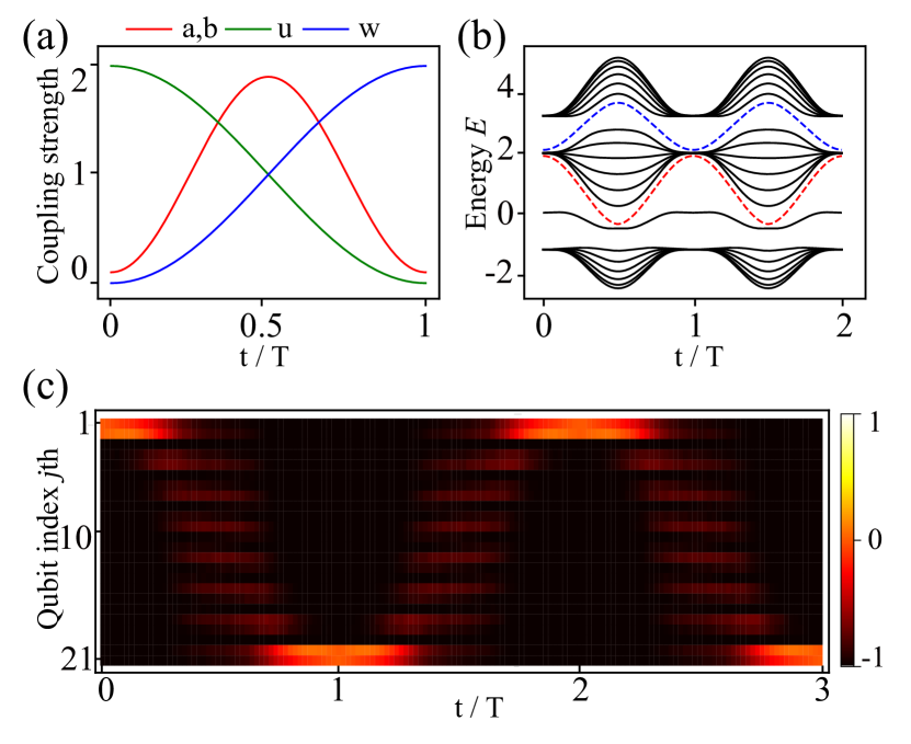
Figure 9: (a) The coupling strengths $a,b$ and on-site potentials $u,w$ versus time $t$. (b) The energy spectrum of the trimer Rice-Mele chain, which contains $3L=21$ qubits. (c) Time evolution of the particle distributions $\langle\sigma_{j}^{z}\rangle$ for the qubit chain. The time-dependent pump sequence is defined in Eq. (34), with $T=1000$. The color from dark-red to bright-yellow represents the particle distribution $\langle\sigma_{j}^{z}\rangle$ varying from $-1$ to $1$.

Figures 9(a) show the time-dependent coupling strengths and on-site potentials versus time $t$ during one period. The initial states are prepared as two-qubit Bell states, i.e., $\left(|e_{1}\rangle\pm|e_{2}\rangle\right)/\sqrt{2}$ in this qubit chain. As shown in Figures 9(b), the two selected topological adiabatic passage are denoted as blue-dashed and red-dashed lines, which can be used to transfer the Exchange-symmetric and Exchange-antisymmetric Bell states. The numerical simulations of the dynamical evolution of the qubit chain prepared in a Bell state is shown in Fig. 9(c). The result shows that the symmetric Bell state can indeed be transferred from one end of the chain to the other end within one pumping cycle. The result of the antisymmetric Bell state is not shown, for the purpose of simplification, because it is identical to the prior example. To ensure the adiabatic limit, we set $T=1000$. As show in the simulation, this pumping process can last for more than three circles. Therefore, we can indeed achieve the edge state pumping in a trimer Rice-Mele model via topological adiabatic passages.

V Discussions and conclusions

V.1 experimental feasibility

Let us now further discuss the experimental feasibility. The qubit-qubit couping in flux qubit circuit can be tuned from 0 to 60 MHz Chen et al. (2014); Geller et al. (2015). Therefore, in our proposal, the state transfer process needs about 10 $\mu s$ for $7$ unit cells for the gap-tunable flux qubit circuit. The coherence time of qubit is about 10-100 $\mu s$ Paik et al. (2011); Novikov et al. (2016), thus it is quite reasonable for execute state transfer process with our protocol. Our proposal can also be realized in other superconducting qubit cirucits, e.g., transmon qubit, which has long coherence time, tunable coupling and frequency modulation. The disadvantage is that anharmonicity is not very good for the transmon qubits, thus the population leakage needs to be considered. In table 1, we list the advantage and disadvantage for two different type of qubit to realize our proposal. We note that the topological magnon insulator states have been experimentally demonstrated in a superconducting circuit with $5$ transmon qubits Cai et al. (2019). Thus it is not very difficult to further study the topological physics using large scale of superconducting quantum circuits with current technology.

QT	CT	TC	FM	Anh
Flux qubit	microseconds	Yes	Yes	Good
Transmon	Several tens seconds	Yes	Yes	Not good

Table 1: Comparisons of the flux and transmon qubits for constructing a qubit chain to realize our proposal. Here, QT, CT, TC, FM and Anh denote Qubit Type, Coherence Time, Tunable Coupling, Frequency modulation, and anharmonicity, respectively.

As for measurements, we can couple the qubit chain dispersively to a microwave resonator. This means the qubits and resonator are detuned in frequency so they do not exchange energy. Applying a microwave pulse at the bare resonator frequency, the pulse will experience a frequency shift and accumulate a phase shift Deac et al. (2008); Béri (2010); Romero et al. (2009); Mallet et al. (2009). By measuring the phase shift of the reflected or transmitted probe pulse, we can infer the state of the qubit.

We note that our qubit chain can be used to implement pumping using one-dimensional Aubry-Andre-Harper (AAH) model Harper (1955); Aubry and André (1980); Lang et al. (2012), which is related to the well-known Hofstadter butterfly problem Hofstadter (1976) in two dimensions. In our proposal, the AAH model can be obtained through the Hamiltonian in Eq. (38), in which the frequency $\omega$ of the $j$th qubit needs to be modulated as $\omega\cos(2\pi j\alpha+t/T)$, where $\alpha$ is a rational (irrational) number. However, the qubit-qubit coupling strengths need to be changed to uniform, i.e., $a=b$. Experimentally, this can be realized by fabricating the chain of coupled superconducting flux qubits with uniform coupling strength, the frequency modulation can be done by applying the magnetic fields through the main loop of each qubit. However, if the coupling strengths of superconducting qubit chain are tunable, then we need only to tune all coupling strengths so that they equal to each other. We further note that the pumping of an edge state based on AAH model was realized in quasicrystals Kraus et al. (2012). Recently, the Hofstadter butterfly spectrum was observed in a chain of nine coupled gmon qubits Roushan et al. (2017).

We mention that the qubit chain can also be constructed using circuit QED system Devoret and Schoelkopf (2013); Gu et al. (2017), where the qubit-qubit coupling can be mediated by the cavity fields. In this case, the cavity fields works as quantum couplers, thus the qubit-qubit coupling can be obtained by eliminating the cavity field with assumption that the qubits and the cavity fields are in the large detuning.

V.2 Conclusions

We have proposed to simulate topological phenomenon using a gap-tunable superconducting-qubit chain, in which the Hamiltonian is equivalent to the SSH model when the total excitations of the qubit chain is limited to one. The spin-up injection at the localized edge state is robust against fluctuations, which can be used to store quantum information. We further show an equivalence of the Rice-Mele model can be realized with the time modulated frequencies and the coupling strengths of the qubit chain, and the adiabatic pumping of an edge state can be realized in this time modulated qubit chain. In our numerical simulation, we take a larger number of the qubits in the chain, e.g., $7$ unit cells. However, we find that the topological phenomena can also be demonstrated in such chain with even smaller qubit number, e.g., $4$ unit cells. We also find that the localization can become more strong with the increase of the qubit number of the chain.

In summary, superconducting quantum circuits can be artificially designed according to the purpose of the experiments. In particular, the qubit frequencies and qubit-qubit couplings can be easily modulated or tuned. This opens many possibilities to simulate or demonstrate various topological physics of matter on demand with artificial designs. We demonstrate that a spin-up state prepared in the one edge of a topological qubit chain can be transferred to the other edge of the chain. This stater transfer process can be interpreted by restricting the Hilbert space of the Hamiltonian into the subspace of the edge states. Thus the hamiltonian of the chain can degenerate to a two-state LZ model, and the state transfer process in the long qubit chain can be easily understood with the adiabatic passage in the LZ model. With this comprehension, we have designed a new approach to achieve the two-qubit Bell state transfer in a trimer Rice-Mele model. Our proposal can also be expended to other tunable quantum system.

Appendix A Gap-tunable flux qubit

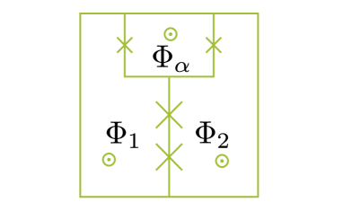
Figure 10: Schematic diagram for the gap-tunable flux qubit. The magnetic flux threading the $\alpha$-loop is denoted by $\Phi_{\alpha}$. $\Phi_{1}$ and $\Phi_{2}$ denote magnetic fluxes through the left and right of the main loop. The signs $\bigodot$ denote that the magnetic fluxes are directed outside.

Let us now briefly summarize the main properties of the gap-tunable flux qubit circuit Paauw et al. (2009); Paauw (2009); Schwarz et al. (2013), which is a variation of a three-junction flux qubit Orlando et al. (1999); Liu et al. (2005a). It replaces the smaller junction in the three-junction flux qubit with a superconducting quantum interference device (SQUID), which is equivalent to a single junction. The SQUID loop is called as $\alpha$-loop. An externally controllable flux $\Phi_{\alpha}$ applied to the $\alpha$-loop can change the Josephson energy of the smaller junction, and the ratio between the larger junctions and the smaller junction is also tunable. This directly results in tunable tunneling between two potential wells of the flux qubit Orlando et al. (1999) and the time modulated frequency of the qubit by applying ac magnetic flux through the $\alpha$-loop. To keep $\Phi_{\alpha}$ from affecting the biased flux threading the main loop, a gradiometric design is adopted. In such design, the central current of the three-junction flux qubit is split into two opposite running currents through two small loops. The magnetic fluxes generated by these two currents cancel each other in the main loop, thus independent control over both fluxes in $\alpha$-loop and main loop is guaranteed. Magnetic fluxes $\Phi_{1}$ and $\Phi_{2}$, applied to two small loops of the qubit, are used to tune the potential well energy of the qubit. Because both the tunneling and the potential well energies can be tuned in the gap-tunable flux qubit, we have a fully controllable Hamiltonian. Below, we use reduced magnetic fluxes $f_{\alpha}=\Phi_{\alpha}/\Phi_{0}$, $f_{\epsilon_{1}}=\Phi_{1}/\Phi_{0}$, and $f_{\epsilon_{2}}=\Phi_{2}/\Phi_{0}$. Here $\Phi_{0}$ is the flux quanta.

We define the flux difference between the two loop halves of the gradiometer as $f_{\epsilon}=f_{\epsilon_{1}}-f_{\epsilon_{2}}$. At the optimal point where $f_{\epsilon}=0$, the low-frequency effect of the environmental magnetic flux reaches minimum, and the two lowest-energy states of the flux qubit are the supercurrents states $\pm I_{p}$ circulating in opposite directions in the $f_{\epsilon}$ loop. In the persistent current states basis, e.g., the anticlockwise current state $|\circlearrowleft\rangle$ and clockwise current state $|\circlearrowright\rangle$, the Hamiltonian of the qubit takes the form (detailed in Appendix D)

$$H=\frac{1}{2}(\epsilon\,\sigma_{x}+\delta\,\sigma_{z}),$$ (35)

where $\sigma_{z}$ and $\sigma_{x}$ are Pauli matrices, the parameter $\delta$ is the tunneling energy between the states of two potential wells and can be tuned by the reduced magnetic flux $f_{\alpha}$. By changing $f_{\alpha}$ and $f_{\epsilon}$, the energy bias $\epsilon(f_{\epsilon},f_{\alpha})=2f_{\epsilon}\Phi_{0}I_{p}(f_{\alpha})$ can be tuned to zero, where the qubit is its optimal point and insensitive to magnetic flux noise to first order. That is, the qubit Hamiltonian in Eq. (35) can be fully controlled by both $f_{\alpha}$ and $f_{\epsilon}$. Moreover, in contrast to the three-junction qubit, in which the transition frequency $\delta$ is fixed at the optimal point, the gap-tunable flux qubit allows us to control the qubit frequency without affecting the bias point, that is, $\delta$ can be tuned by $f_{\alpha}$ even at the optimal point with $f_{\epsilon}=0$. This is demonstrated in detail in the appendix. Moreover, if a time-dependent magnetic flux with the frequency $\omega_{0}$ is applied to the $\alpha$-loop, a time-dependent longitudinal coupling Zhou et al. (2009); Liu et al. (2014) Hamiltonian $\lambda_{z}\sigma_{z}\cos(\omega_{0}t)/2$ with the coupling constant $\lambda_{z}$ between the qubit and external field should be included, then the qubit Hamiltonian in Eq. (35) becomes into

$$H^{\prime}=\frac{1}{2}(\epsilon\,\sigma_{x}+\delta\,\sigma_{z})+\frac{1}{2}\lambda_{z}\cos(\omega_{0}t)\sigma_{z}.$$ (36)

In the qubit basis corresponding to the excited $|e\rangle$ and ground $|g\rangle$ states of the Hamiltonian in Eq. (35), we can derive the longitudinal and the transverse couplings between the qubit and external field from Eq. (36). However, if the qubit works at the optimal point with $\epsilon=0$, then the time dependent Hamiltonian in Eq. (36) becomes into

$$H^{\prime}=\frac{1}{2}\delta\,\sigma_{z}+\frac{1}{2}\lambda_{z}\cos(\omega_{0}t)\sigma_{z}=\frac{1}{2}[\delta+\lambda_{z}\cos(\omega_{0}t)]\sigma_{z},$$ (37)

which has only longitudinal coupling. Here, we note that the coupling constant $\lambda_{z}$ can be negative or positive by choosing the initial phase of the time-dependent external magnetic flux. This Hamiltonian can also be explained as that the qubit frequency is periodically modulated by the external field. This longitudinal coupling can result in the decoupling of the qubit from its environment.

Appendix B Periodic Superconducting qubit chains

As shown in Fig. 10, there are four current loops in the gap-tunable flux qubit, thus different types of tunable couplings can be created via different loops. For example, the longitudinal coupling $\sigma_{j}^{z}\sigma_{j+1}^{z}$ between the $j$th and $(j+1)$th qubits in the qubit chain can be realized by inductively coupling them through their $\alpha$-loops Billangeon et al. (2015). However, in this paper, we mainly focus on the transverse coupling $\sigma_{j}^{x}\sigma_{j+1}^{x}$ between the qubits via $\epsilon$-loops. Here, $\sigma_{j}^{x}$, $\sigma_{j}^{y}$, and $\sigma_{j}^{z}$ denote Pauli operators, which are defined in the qubit basis $|g\rangle_{j}$ and $|e\rangle_{j}$ of the $j$th qubit.

To demonstrate different topological physics with gap-tunable flux qubits, in this section, we mainly show how to realize two coupling mechanism between gap-tunable flux qubits. (i) The qubits are directly coupled to each other via a mutual inductance, with fixed coupling strengths between qubits, but the frequencies of qubits can be either modulated or fixed. (ii) The qubits are indirectly coupled to each other via a coupler, thus both the qubit frequencies and the coupling strengths between qubits can be controlled. The first approach might be experimentally challenging, but the second one is more popular in recent experiments.

B.1 Qubit chain with fixed coupling strength

As schematically shown in  Fig. 11, the qubits in the chain can be directly coupled to each other, that is, $2N$ identical gap-tunable flux qubits in the chain are directly coupled to each other through their mutual inductance via $\epsilon$-loops. We assume that each qubit is only coupled to its nearest neighbors, the coupling strength between $j$th and $(j+1)$th qubits can be obtained by $J=MI_{pj}I_{p(j+1)}$. Here $M$ is the mutual inductance between the $j$th and $(j+1)$th qubit loops, $I_{pj}$ and $I_{p(j+1)}$ are the current circulating main loops of the $j$th and $(j+1)$th qubits. Projecting $J$ onto the eigenstates of the $j$th and $(j+1)$th qubits, i.e., the states $|g\rangle_{j}$, $|g\rangle_{j+1}$, $|e\rangle_{j}$, and $|e\rangle_{j+1}$, we can obtain the coupled Hamiltonian, which includes the longitudinal coupling term $\sigma_{j}^{z}\sigma_{j+1}^{z}$ with the coefficient $g^{zz}_{j,j+1}$, transverse coupling term $\sigma_{j}^{x}\sigma_{j+1}^{x}$ with the coefficient $g^{xx}_{j,j+1}$ , and cross coupling terms, e.g., $\sigma_{j}^{x}\sigma_{j+1}^{z}$ with the coefficient $g^{xz}_{j,j+1}$. Detailed analysis in the Appendix shows that the interaction via the main loops only results in transverse coupling when the qubits work at the optimal point, while the coefficients $g^{zz}_{j,j+1}$ and $g^{zx}_{j,j+1}$ of the longitudinal and cross couplings are zero.

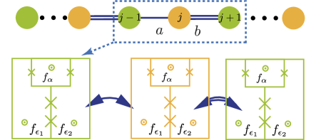
Figure 11: Schematic diagram for the chain of coupled gap-tunable flux qubits with alternating coupling strengths $a$ and $b$ (Top panel). As shown in the lower panel, each qubit is coupled to its nearest-neighbors via the flux $f_{\epsilon_{i}}$. The different coupling strengths $a$ and $b$ are created by varying the spacing between the qubits. The frequency of the qubit can be tuned in situ by the magnetic frustration $f_{\alpha}$ threading the $\alpha$-loop.

To make the qubit have long coherence, we assume that all gap-tunable qubits in the chain work at the optimal point in the following discussions, then there is only transverse coupling between the qubits. As shown in the Appendix, the coupling coefficient $g^{xx}_{j,j+1}$ of the transverse coupling between the $j$th and $(j+1)$th qubits is written as $g^{xx}_{j,j+1}=Mg^{j}_{\epsilon,\bot}g^{j+1}_{\epsilon,\bot}$, with $g^{j}_{\epsilon,_{\bot}}={{}_{j}\langle e|I_{pj}|g\rangle}_{j}$ and $g^{(j+1)}_{\epsilon,_{\bot}}={{}_{j+1}\langle e|I_{p(j+1)}|g\rangle}_{j+1}$. To create alternating coupling pattern as schematically shown in Fig. 10, the spacings between the qubits need to be varied respectively in order to alter $M$. This is experimentally accessible with current technology of the superconducting qubit circuits. The qubit chain is fabricated such that $a\equiv g^{xx}_{(2m-1),2m}$ and $b\equiv g^{xx}_{2m,(2m+1)}$ with $m=1,\,2,\cdots,L$. We note that $b=0$ when $m=L$. Then, the Hamiltonian of the coupled-qubit chain can be written as

$$H = \sum_{j=1}^{2N}\frac{\omega_{j}}{2}\sigma_{j}^{z}+\sum\limits_{{j\in\mathrm{odd}}}^{2N}a(\sigma_{j}^{+}\sigma_{j+1}^{-}+{\text{H}.c.})$$ (38)

$$+ \sum\limits_{{j\in\mathrm{even}}}^{2N}b(\sigma_{j}^{+}\sigma_{j+1}^{-}+{\text{H}.c.}),$$

with $\omega_{j}$ denoting the frequency of the qubit. Because we assume that all qubits are identical, thus the qubits have the same frequency, that is, $\omega_{j}=\omega$ with $j=1,\cdots,2N$. That is, the qubits resonantly interact with each other, and then we can make rotating wave approximation such that the transverse coupling term $\sigma_{j}^{x}\sigma_{j+1}^{x}$ between the $j$th and $(j+1)$th qubits is approximated as $\sigma_{j}^{x}\sigma_{j+1}^{x}\approx(\sigma_{l}^{+}\sigma_{l+1}^{-}+\sigma_{j}^{-}\sigma_{j+1}^{+})$. It is clear that the coupling strengths $a$ and $b$ are fixed once the circuit is fabricated.

As shown in Fig. 11 and discussed in Section A, when the qubit works at the optimal point, the frequency modulation can be only done by applying the time-dependent magnetic flux through the $\alpha$-loop. However, when all the qubits do not work at the optimal point, although the frequency of each qubit and the coupling strength between the qubits can be modulated by a time-dependent magnetic flux applied through the main loop of each qubit Liu et al. (2006), the coherence of the qubits becomes worse. Thus, hereafter, we assume that the all qubits work at their optimal points. The qubit readout and control can be done in principle as in experiments Paauw et al. (2009); Paauw (2009); Schwarz et al. (2013). In practise, there exists the next-nearest neighbor coupling in all superconducting circuits of many qubits with either capacitive or inductive coupling, these couplings can be minimized to be negligibly small by carefully designing circuits, e.g., as in the superconducting flux qubit chain with direct inductive coupling Paauw (2009).

In above, we construct a qubit chain with fixed coupling. If the coupling between qubits in the chain can be tuned, then the system can be tuned from topological to non-topological phase, vice versa. In the natural atomic systems, the coupling is not tunable. However, the superconducting systems provide us ability to tune the coupling between the qubits. Below, we show two ways to tune the couplings between qubits in the chain.

B.2 Qubit chain with tunable couplings

In superconducting qubit circuits, the tunable coupling can be realized by using many methods. In this section, we show two methods, which are used for tunable coupling. One is that the qubit coupling can be tuned by modulating qubit frequencies with longitudinal coupling fields as shown in Eq. (37). Another one is tunable coupling realized by adding the additional coupler between qubits.

B.2.1 tunable coupling realized by longitudinal coupling field

We now show how to tune the coupling by modulating the qubit frequencies. We assume that all flux qubits in the chain work at their optimal points, thus the qubit frequency can be modulated by applying the magnetic flux through the $\alpha$-loop as shown in Refs. Goetz et al. (2018); Wang et al. (2018). In this case, the Hamiltonian $\omega_{j}\sigma_{j}^{z}/2$ of the single qubit in Eq. (38) is replaced by the modulated Hamiltonian in Eq. (37), and the Hamiltonian in Eq. (38) can be written as

$$H_{M} = \sum_{j=1}^{2N}\frac{\omega_{j}+{u_{j}}(t)}{2}\sigma_{j}^{z}+\sum\limits_{{j\in\mathrm{odd}}}^{2N}\left[a(\sigma_{j}^{+}\sigma_{j+1}^{-}+\sigma_{j}^{-}\sigma_{j+1}^{+})\right]$$ (39)

$$+ \sum\limits_{{j\in\mathrm{even}}}^{2N}\left[b(\sigma_{j}^{+}\sigma_{j+1}^{-}+\sigma_{j}^{-}\sigma_{j+1}^{+})\right].$$

with $u_{j}(t)=\lambda_{j}\cos(\omega_{0j}t)$. Here, $\lambda_{j}$ is proportional to the strength of the driving field and $\omega_{0j}$ is the frequency of the driving field. For convenience, we also assume that the initial phases of all driving fields are zero. We now apply a unitary transformation $U(t)=\bigotimes U_{j}(t)$ to Eq. (39) with Liu et al. (2014).

$$U_{j}(t)=\exp\left[-\frac{i}{2}\left(\omega_{j}t+\frac{\lambda_{j}}{\omega_{0j}}\sin(\omega_{0j}t)\right)\sigma_{j}^{z}\right]$$ (40)

then we find that the term $u_{j}(t)$ in Eq. (39) is canceled, and then operators $\sigma_{j}^{\pm}$ become into

$$U^{\dagger}_{j}(t)\sigma_{j}^{\pm}U_{j}(t) = \sigma_{j}^{\pm}\exp\left[\pm i\left(\omega_{j}t+\frac{\lambda_{j}}{\omega_{0j}}\sin(\omega_{0j}t)\right)\right]$$

$$= \sum_{n=-\infty}^{\infty}i^{n}\exp[\pm i(\omega_{j}+n\omega_{0j}t]J^{j}_{n}\left(\pm\alpha_{j}\right)$$

with $\alpha_{j}\equiv\lambda_{j}/\omega_{0j}$ and the Bessel functions $J^{j}_{n}\left(\pm\alpha_{j}\right)$ of the first kind. Here, $j$ is the index of the $j$th qubit.

If all the qubits are identical and the frequencies of the driving fields are the same, that is, $\omega_{j}=\omega$ and $\omega_{0j}=\omega_{0}$ with $j=1,\cdots,2N$, then the Hamiltonian in Eq. (39) becomes into an effective Hamiltonian

$$H_{1}=\sum\limits_{{j\in\mathrm{odd}}}^{2N}\left[P\sigma_{j}^{+}\sigma_{j+1}^{-}+{\text{H}.c.}\right]+\sum\limits_{{j\in\mathrm{even}}}^{2N}\left[Q\sigma_{j}^{+}\sigma_{j+1}^{-}+{\text{H}.c.}\right].$$

with effective coupling strengths

$$P = a\sum_{n=-\infty}^{\infty}(-1)^{n}J_{n}^{j}(\alpha_{j})J_{n}^{(j+1)}(\alpha_{j+1}),$$ (43)

$$Q = b\sum_{n=-\infty}^{\infty}(-1)^{n}J_{n}^{j}(\alpha_{j})J_{n}^{(j+1)}(\alpha_{j+1}),$$ (44)

after all oscillation terms of high frequencies are neglected. Here, $j$ takes odd and even numbers for coefficients $A$ and $B$, respectively. It is clear that the coefficients $A$ and $B$ can be tuned by changing ratios $\alpha_{j}\equiv\lambda_{j}/\omega_{0j}$ through the amplitudes of driving fields when the frequencies $\omega_{0j}$ are given.

However, in practise, the qubit frequencies are not exactly same, this provides us more convenient way to tune the coupling strength via frequency matching Liu et al. (2006). If we assume that $\omega_{j}-\omega_{j-1}=\omega_{0j}$ for odd number $j$ and $\omega_{j}-\omega_{j-1}=\omega_{0(j-1)}$ for even number, then the effective Hamiltonian can be written as

$$H_{2}=\sum\limits_{{j\in\mathrm{odd}}}^{2N}\left[A^{\prime}\sigma_{j}^{+}\sigma_{j+1}^{-}+{\text{H}.c.}\right]+\sum\limits_{{j\in\mathrm{even}}}^{2N}\left[B^{\prime}\sigma_{j}^{+}\sigma_{j+1}^{-}+{\text{H}.c.}\right].$$

with effective coupling strengths

$$P = iaJ_{0}^{j}(\alpha_{j})J_{1}^{(j+1)}(\alpha_{j+1}),$$ (46)

$$Q = ibJ_{1}^{j}(\alpha_{j})J_{0}^{(j+1)}(\alpha_{j+1}),$$ (47)

which has been experimentally demonstrated in a qubit chain with five transmon qubits Li et al. (2018) and also two coupled qubits Wang et al. (2018). Therefore, tunable couplings between qubits can be realized by modulating the qubit frequencies without increasing the complexity of the circuit.

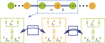
Figure 12: Couplers (rectangle) are inserted between qubits in the chain to achieve time-dependent tunable coupling strengths. The couplers can be superconducting quantum interference devices, superconducting qubits, LC circuits, or other superconducting elements.

B.2.2 tunable coupling via couplers

If the qubits work at the optimal point and their frequencies are not modulated, then as schematically shown in  Fig. 12, additional couplers Liu et al. (2006, 2007); Grajcar et al. (2006); Rigetti et al. (2005); Bertet et al. (2006); Niskanen et al. (2006) can be used to achieve tunable couplings between the qubits. Various couplers have been demonstrated in the two-qubit cases Liu et al. (2006, 2007); Grajcar et al. (2006); Rigetti et al. (2005); Bertet et al. (2006); Niskanen et al. (2006); Hime et al. (2006); Niskanen et al. (2007); Harris et al. (2007); van der Ploeg et al. (2007); Allman et al. (2010); Bialczak et al. (2011) and can be extended to large scale of qubit circuits. In this case, using the same procedure for the directly coupled qubit chain in Fig. 11, we can write out the full Hamiltonian of the qubit chain, in which each pair of qubit is indirectly coupled through their coupler. The effective couplings between qubits can be obtained after the variables of the couplers are eliminated.

The coupler can work at either classical or quantum regime. When the couplers work at the classical regime, the variables of the couplers can be adiabatically eliminated as discussed in Ref. Grajcar et al. (2006). When the couplers work at the quantum regime, we usually assume that the transition frequency from the ground to first excited state of the coupler is much larger than the qubit frequencies. Then we can eliminate the variables of the couplers by the large detuning approximation Liu et al. (2005b). In either way, we can obtain an effective Hamiltonian as

$$H_{C} = \sum\limits_{{j\in\mathrm{odd}}}^{2N}\left[\frac{\omega^{\prime}_{j}}{2}\sigma_{j}^{z}+a(t)(\sigma_{j}^{+}\sigma_{j+1}^{-}+\sigma_{j}^{-}\sigma_{j+1}^{+})\right]$$

$$+ \sum\limits_{{j\in\mathrm{even}}}^{2N}\left[\frac{\omega^{\prime}_{j}}{2}\sigma_{j}^{z}+b(t)(\sigma_{j}^{+}\sigma_{j+1}^{-}+\sigma_{j}^{-}\sigma_{j+1}^{+})\right],$$

which has the same form as in Eq. (38) . However, here the parameters $a(t)$ and $b(t)$ are time-dependent..

There are differences between Eq. (38) and Eq. (B.2.2). The bare qubit frequency $\omega$ in Eq. (38) is modified to $\omega_{j}^{\prime}$ in Eq. (B.2.2) when the couplers are eliminated. The effective coupling strengths between qubits induced by couplers are tunable now and can be denoted by time-dependent parameters $a(t)$ and $b(t)$. The tunable coupling strengths between qubits are realized by individually applying the magnetic flux through the loop of each coupler. For the coupler which works in the quantum regime, the applied magnetic flux changes the frequency of the coupler such that the detuning between quibts and coupler is changed, and then the effective coupling between qubits is changed with the change of applied magnetic flux. For the coupler which works in the classical regime, the magnetic flux changes the effective mutual inductance between the qubits, and then the coupling strength is changed. Therefore, in both the cases, we can consider that the effective coupling strengths are time-dependent.

Here we further note that if the qubit frequency is also modulated for the qubit with the coupler, then we can obtain an effective Hamiltonian with both the tunable coupling and qubit frequency modulation. Such full controlled circuit enables us to demonstrate various one-dimensional topological model.

Appendix C Topologically protected solitons

We now study how the proposed superconducting qubit chain with Hamiltonian in Eq. (38) can be used to demonstrate topologically protected solitons when there is only a single-excitation in $2N$ superconducting qubits. To clearly illustrate this, let us fix the coupling strength between the even qubit and its right neighbor, e.g., hereafter we take the coupling strength $b$ as a unit, i.e., $b=1$. Then we study how the hopping amplitude $a$, the hopping strength between the odd qubit and its right neighbor, affects the energy spectrum and the topological properties of the chain.

In our simulation, for concreteness, the total number of superconducting qubits is set as $2N=14$. We plot, in Fig. 13(a), the energy spectrum of the Hamiltonian in Eq. (3) and corresponding eigenfunctions $|\psi_{l}\rangle$ where $l=1,\cdots,2N$ in the basis $|e_{j}\rangle$ shown in Eq. (2). They are plotted in Figs. 13(b) and (c) with $a=0.1$, in Fig. 13(d) with $a=1$. Here, emphasize that the tunable coupling strengths $a$ and $b$ can be realized via frequency modulation or couplers as shown in above studies..

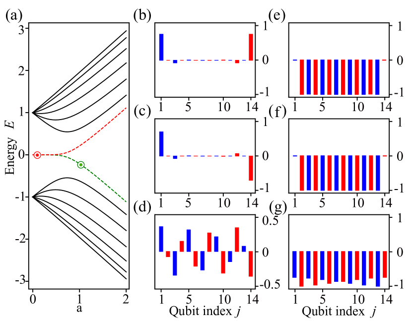
Figure 13: Spectrum and wave functions of the Hamiltonian (3). The total number of qubits is assume as $14$. (a) Energy spectrum verses the coupling strength $a$ with $b=1$. Degenerate wave functions, corresponding to the zero-energy mode with $a=0.1$ indicated by a red point in (a), are shown in (b) and (c), respectively. A typical bulk state at the point $a=1$, marked by a green point in (a), is plotted in (d). The observables $\langle\sigma_{n}^{z}\rangle$ of the corresponding wave functions in (b), (c) and (d), are shown in (e), (f) and (g). All the navy blocks denote the amplitude on the odd qubits, while the red blocks represent the even sites.

Figure 13 bears several interesting features. (i) Due to the bipartite lattice structure, the spectrum exhibits two band. (ii) The spectrum is symmetric around zero. For any state with energy $E$, there is a partner with energy $-E$. This stems from the chiral symmetry of the SSH model Asbóth et al. (2016). (iii) For the $E\neq 0$ states, all the wave functions have support on both even and odd qubits, also known as the bulk states. Figure 13(d) shows a typical bulk state wave function corresponding to the point $a=b=1$ marked by a red point in Fig. 13 (a). (iiii) There is a zero energy ($E=0$) mode lying in the middle of the bulk gap, where $a<b$. The zero-energy mode has two degenerate states. They are presented in Fig. 13 (b) and (c) corresponding to $a=0.1$ point marked by a star in Fig. 13 (a). The eigenfunctions are localized at the left and right edge, and decay exponentially towards the bulk.

The appearance of $E=0$ mode with localized eigenfunctions is the key feature of the topological phase when $a<b$. The localized eigenfunctions shown in Figs.13(b) and (c) are the superpositions $|L\rangle\pm|R\rangle$ of the left and right edge states $|L\rangle$ and $|R\rangle$. Here the left edge state is defined as

$$|L\rangle=\sum\limits_{j\in\mathrm{odd}}a_{j}|e_{j}\rangle,$$ (49)

where $j$ is an odd number and $a_{j}$ is the amplitude on the odd qubits. Similarly, the right edge state is written as

$$|R\rangle=\sum\limits_{j\in\mathrm{even}}b_{j}|e_{j}\rangle,$$ (50)

here $j$ is an even number and $b_{m}$ is the amplitude on the even qubits. Note the vanishing amplitudes on the even (odd) site of the left (right) edge state are the consequence of the chiral symmetry. The decay depth into the bulk is characterized by Asbóth et al. (2016)

$$|a_{j}|=|a_{1}|{\rm exp}\left(-\frac{j-1}{2\xi}\right),$$ (51)

where the localization length $\xi=(\ln|b|-\ln|a|)^{-1}$. When the ratio $|b|/|a|$ becomes appreciably large, the wave function will almost be confined at the first and last qubit.

The particle distributions in the eigenfunctions $|\psi_{l}\rangle$ of the qubit chain can be measured via the variable $\sigma_{n}^{z}$ of each qubit, with the measurement result $\langle\psi_{l}|\sigma_{n}^{z}|\psi_{l}\rangle$. Here, the subscript $n$ denotes the $n$th qubit. We note that the in the single-excitation subspace, the Pauli operator $\sigma_{n}^{z}$ can be expressed as $\sigma_{n}^{z}=2|e_{n}\rangle\langle e_{n}|-I$, where $I$ is the identity matrix. Although the qubits are coupled to each other, the excitation stays at the end of qubit chain as shown in Fig. 13 (e) and (f).

To demonstrate the existence of edge states, we study the quench dynamics after the first qubit is flipped. That is, let us assume that all the qubits are initially in the spin-down state, then a $\pi$ pulse is applied to flip the first qubit. The dynamics of the qubit chain can be measured by

$$\langle\sigma_{n}^{z}(t)\rangle=\langle e_{1}|e^{iH_{\mathrm{S}}t}\sigma_{n}^{z}e^{-iH_{\mathrm{S}}t}|e_{1}\rangle.$$ (52)

with the Hamiltonian given in Eq. (3). Below, we compare the dynamics of a topological SSH chain, described by the Hamiltonian in Eq. (3) when $a=0.1$ and $b=1$, with a transverse spin chain, described by the Hamiltonian in Eq. (3) when $a=b=1$.

To model the small divergence of the qubits resulted from the sample fabrication, a random noise $\eta$ is introduced to the coupling strengths $a$ and $b$, as well as the frequency $\omega$ in Eq. (3). Here $\eta$ follows Gaussian distribution with mean value $0$, and a standard deviation $0.01$. That is the fluctuations of the coupling strength and qubit frequencies are $10\%$ of the smaller coupling strength $a$.

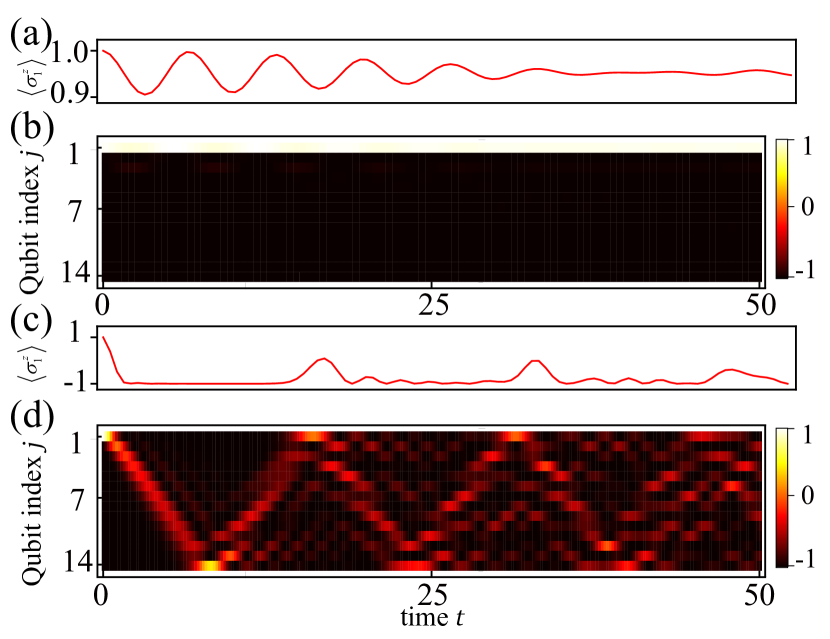
Figure 14: Time evolution of $\langle\sigma_{j}^{z}\rangle$, after the first qubit is flipped to the spin-up state. (a) and (c) show the time evolution $\langle\sigma_{1}^{z}\rangle$ of the first qubit. (b) and (d) show the time evolution $\langle\sigma_{i}^{z}\rangle$ of all the qubits. A random noise with an amplitude of $10\%$ of the coupling strength $a$ is added to the qubit frequency and coupling strength. The topological SSH chain with $a=0.1$ and $b=1$ is shown in (a) and (b). The transverse Ising chain with $a=b=1$ is plotted in (c) and (d). In our plot, the qubit number in the chain is assumed as $14$.

For the topological SSH chain with $a=0.1$ and $b=1$ in the Hamiltonian of Eq. (3), Fig. 14(a) and (b) show that the excitation remains as a soliton at the first qubit. This can be understood by the evolution of the wave function

$$|\psi(t)\rangle=\sum_{l}e^{-E_{l}t/\hbar}\langle\psi_{l}|e_{1}\rangle|\psi_{l}\rangle,$$ (53)

where $|\psi_{l}\rangle$ denotes the $l$th eigenfunctions of the Hamiltonian in Eq. (3) with corresponding eigenenergy $E_{l}$. We start with the state $|e_{1}\rangle$ after the excitation is injected at the first qubit. $|e_{1}\rangle$ has a substantial overlap with the degenerate edge states with corresponding eigenenergy $E=0$. This leads to a stationary state. Conversely, if we inject the excitation in the transverse Ising chain described by the Hamiltonian of Eq. (3) with $a=b=1$, without localized edge states, it will quickly diffuse into the bulk. This can be seen from Figs. 14(c) and (d). The excitation at the first qubit quickly expands into the bulk, reaches the end of the qubit chain, and then is reflected back. The similar propagation of such excitations is demonstrated in Refs. Viehmann et al. (2013a, b).

In summary, due to the alternating coupling pattern $a<b$ of the whole chain, the soliton is topologically protected and robust against disorder. This is because the soliton resides in the gap, extra energy is required if we want to excite the soliton to other states. We have also shown the random noise added to the parameters in Eq. (38) have no appreciable influence on the soliton state.

Though the soliton appears at the very end of the chain, it can also be created at the interface between the topological phase with $a<b$ and topologically trivial phase with $a>b$. For example, as shown in Ref. Estarellas et al. (2017), if a defect is created at the center of a topological SSH chain, then a zero energy mode localizes at the defect. Moreover, the defect can serve as a high-fidelity memory, which is topologically protected. An arbitrary state encoded with the presence and absence of the localized state can allow for perfect state transfer in the spin chain Estarellas et al. (2017); Bose (2003).

Appendix D Hamiltonian derivation of the gap-tunable flux qubit

In this section, the Hamiltonian of inductively coupled gap-tunable flux qubit (Fig. 10) will be derived. With our design, the qubit frequencies and the couplings between qubits (e.g. in Eq. (38)) can be tailored and tuned in situ by external fluxes.

D.1 Hamiltonian of single qubit

A Gap-tunable flux qubit Paauw et al. (2009); Paauw (2009); Schwarz et al. (2013), as shown in Fig. 15, replaces the $\alpha$ junction of a three-junction flux qubit Orlando et al. (1999) with a SQUID. This introduces an external controllable flux $f_{\alpha}$ to tune $\alpha$ in situ, thus changing the gap (qubit frequency). To keep $f_{\alpha}$ from affecting the biasing flux $f_{\epsilon}$ threading the main loop, a gradiometric design is adopted. In this $8$-shaped design, the central current of the three-junction flux qubit is split into two opposite running currents. Because the magnetic flux generated by these two currents now cancel each other in the main loop, independent control over both flux $f_{\alpha}$ and $f_{\epsilon}$ is ensured. Different types of tunable couplings can also be created via different loops. For example, longitudinal coupling between two qubits ($\sigma_{l}^{z}\sigma_{l+1}^{z}$) can be realized by inductively coupling two qubits through their $f_{\alpha}$-loop Billangeon et al. (2015). In this paper, we focus on the transverse coupling ($\sigma_{l}^{x}\sigma_{l+1}^{x}$) through the $f_{\epsilon}$-loop.

We follow the notations in Refs. Paauw (2009); Billangeon et al. (2015), as shown in Fig. 15. We assume the phase accumulated along the main trap-loop is $\theta$. Here $\beta$ denotes the ratio between the circumference of the $\alpha$-loop to the main trap-loop. The magnetic frustration threading the corresponding loop is denoted by $f_{i}$. The phase difference across the junction is $\varphi_{i}$.

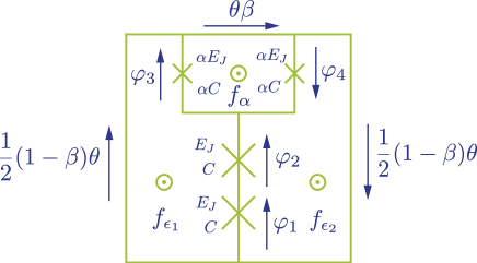
Figure 15: Circuit representation of a gap tunable flux qubit. The sign $\times$ denotes the Josephson junction. The long arrows denote the current direction. The phase accumulated along the main trap-loop is denoted by $\theta$. The parameter $\beta$ denotes the ratio between the circumference of the $\alpha$-loop and that of the main trap-loop. The $f_{\alpha}=\Phi_{\alpha}/Phi_{0}$ denotes the reduced magnetic flux threading the $\alpha$ loop, and $f_{1}=\Phi_{1}/\Phi_{0}$ and $f_{2}=\Phi_{2}/\Phi_{0}$ denote the reduced magnetic fluxes through the left and right parts of the main loop, respectively. $E_{J}$ and $C_{J}$ denote the Josephson energy and capacitance, respectively. The phase difference across each junction is denoted by $\varphi_{i}$.

Then the flux quantization conditions for the main trap-loop, $\alpha$-loop, $f_{\epsilon_{1}}$-loop, $f_{\epsilon_{2}}$-loop are

$$\theta+2\pi(f_{\epsilon_{1}}+f_{\epsilon_{2}}+f_{\alpha})=2\pi N$$

$$\varphi_{3}+\varphi_{4}+\beta\theta+2\pi f_{\alpha}=2\pi N_{\alpha}$$

$$\frac{1}{2}(1-\beta)\theta-\varphi_{3}-\varphi_{2}-\varphi_{1}+2\pi f_{\epsilon_{1}}=2\pi N_{1}$$

$$\frac{1}{2}(1-\beta)\theta+\varphi_{1}+\varphi_{2}-\varphi_{4}+2\pi f_{\epsilon_{2}}=2\pi N_{2},$$ (54)

where $N_{i}$ is the number of trapped fluxoids.

Using above conditions, $\varphi_{3}$, $\varphi_{4}$ can be expressed in terms of $\varphi_{1}$, $\varphi_{2}$,

$$\varphi_{3}=-\pi[\beta(N-f_{\Sigma})+f_{\alpha}]-(\varphi_{1}+\varphi_{2})-\pi(n-f_{\epsilon})+\pi N_{\alpha},$$

$$\varphi_{4}=-\pi[\beta(N-f_{\Sigma})+f_{\alpha}]+(\varphi_{1}+\varphi_{2})+\pi(n-f_{\epsilon})+\pi N_{\alpha},$$

where $f_{\Sigma}=f_{\epsilon_{1}}+f_{\epsilon_{2}}+f_{\alpha}$, $f_{\epsilon}=f_{\epsilon_{1}}-f_{\epsilon_{2}}$, $N=N_{1}+N_{2}+N_{\alpha}$, $n=N_{1}-N_{2}$. For simplicity, we assume $N_{\alpha}=0$ in the following analysis.

Following the standard circuit quantization process Devoret (1995); Wendin and Shumeiko (2005), the charging energy of the capacitor represents the kinetic energy, while the Josephson energy represents the potential energy. Then the Lagrangian of the circuit in terms of $\varphi_{1}$, $\varphi_{2}$ is

$$\mathscr{L} (\dot{\varphi_{i}},\varphi) =$$

$$(\frac{\hbar}{2e})^{2} [(1+2\alpha)\frac{C}{2}(\dot{\varphi_{1}}^{2}+\dot{\varphi_{2}}^{2})+2\alpha C\dot{\varphi_{1}}\dot{\varphi_{2}}]$$

$$-E_{J} (2(1+\alpha)-\cos\varphi_{1}-\cos\varphi_{2}-$$

$$2\alpha\cos \{\pi[\beta(N-f_{\Sigma})+f_{\alpha}]\}\cos[(\varphi_{1}+\varphi_{2})+\pi(n-f_{\epsilon})]).$$

The canonical momentum $p_{i}$ conjugated to coordinate $\varphi_{i}$ is

$$p_{1}=\frac{\partial L}{\partial\dot{\varphi_{1}}}=(\frac{\hbar}{2e})^{2}[(1+2\alpha)C\dot{\varphi_{1}}+2\alpha C\dot{\varphi_{2}}],$$

$$p_{2}=\frac{\partial L}{\partial\dot{\varphi_{2}}}=(\frac{\hbar}{2e})^{2}[(1+2\alpha)C\dot{\varphi_{2}}+2\alpha C\dot{\varphi_{1}}].$$ (57)

The Hamiltonian is related to the Lagrangian by Legendre transformation

$$H(p_{i},\varphi_{i}) =\sum p_{i}\dot{\varphi}_{i}-\mathscr{L}$$

$$= \frac{4E_{C}}{(1+4\alpha)}[(1+2\alpha)n_{1}^{2}-4\alpha n_{1}n_{2}+(1+2\alpha)n_{2}^{2}]$$

$$+E_{J}( 2(1+\alpha)-\cos\varphi_{1}-\cos\varphi_{2}$$

$$-2\alpha\cos \{\pi[\beta(N-f_{\Sigma})+f_{\alpha}]\}\cos[(\varphi_{1}+\varphi_{2})+\pi(n-f_{\epsilon})]),$$

where charging energy of the junction is defined as $E_{C}=e^{2}/2C$. We also introduced the number operator of Cooper-pairs on the junction capacitor $n_{i}=p_{i}/\hbar$, which can also be written as $n_{i}=-i\partial/\partial\varphi_{i}$.

htp

Figure 16: (a) Dependence of energy levels on the frustration $f_{\epsilon}$, with $f_{\alpha}=0.2$. (b) The energy gap $\omega$ as a function of $f_{\alpha}$ when biased at the optimal working point $f_{\epsilon}=0$. (c) Longitudinal coupling strength through $f_{\epsilon}$ loop, with $f_{\alpha}=0.2$. (d) Transverse coupling strength through $f_{\epsilon}$ loop, with $f_{\alpha}=0.2$. The rest parameters are $E_{J}=1$, $E_{J}/E_{C}=50$, $\alpha=0.5$, $f_{\Sigma}=50f_{\alpha}$, $\beta=0.05$, $N=1$, $n=1$.

The energy levels of the qubit are solved numerically by the plane-wave solutions $\Psi(\varphi_{1},\varphi_{2})=\frac{1}{2\pi}\sum_{k,l=-N}^{N}c_{k,l}\exp\{-i(k\varphi_{1}+l\varphi_{2})\}$. Here $k$ ($l$) is an integer, corresponding to a state that has $k$ ($l$) Cooper pairs on junction $1$ ($2$). The total charge states is set to $N=15$.

The energy levels as a function of the bias flux $f_{\epsilon}$ are plot in Fig. 16 (a). At the optimal working point where $f_{\epsilon}=0$, the lowest two energy levels is well separated from higher excited states. The splitting of these two levels is the qubit frequency $\omega$. As shown in Fig. 16 (b), $\omega$ can be tuned by $f_{\alpha}$.

D.2 Qubit-qubit coupling

As shown in Fig. 10, the qubits are coupled inductively via $f_{\epsilon}$-loop. The current $I_{p,j+1}$ circulating the $f_{\epsilon}$ loop of the $j+1$th qubit can induce a change of flux $\delta f_{j}$ in the $f_{\epsilon}$ loop of qubit $j$, giving rise to the coupling term $J=MI_{pj}I_{p(j+1)}$, where the current $I_{pj}=\partial\mathscr{H}_{j}/\partial f_{\epsilon}$. Here we assume $\delta f_{j}$ does not affect $f_{\alpha}$-loop.

As shown in the main text, the transverse coupling strength $a=g^{j}_{\epsilon,\bot}g^{j+1}_{\epsilon,\bot}$, with

$$g_{\epsilon,\bot}=\langle e|\frac{\partial\mathscr{H}}{\partial f_{\epsilon}}|g\rangle.$$ (60)

For simplicity we have dropped the superscript $j$.

Similarly the longitudinal coupling $\lambda\sigma_{j}^{z}\sigma_{j+1}^{z}$ is also possible, where $\lambda=g^{j}_{\epsilon,\|}g^{j+1}_{\epsilon,\|}$, with

$$g_{\epsilon,\|}=\langle+|\frac{\partial\mathscr{H}}{\partial f_{\epsilon}}|-\rangle.$$ (61)

Here $|\pm\rangle=(|e\rangle\pm|g\rangle)/\sqrt{2}$.

Note because of the gradiometric geometry, the flux in the main trap loop is insensitive to a homogeneous magnetic field. Thus only the asymmetrical flux $f_{\epsilon}=f_{\epsilon_{1}}-f_{\epsilon_{2}}$ contributes in the coupling.

We plot $g_{\epsilon,\|}$ and $g_{\epsilon,\bot}$ as a function of the bias flux $f_{\epsilon}$ in Fig. 16 (c) and (d). At the optimal working point $f_{\epsilon}=0$, $g_{\epsilon,\bot}$ is the largest, while $g_{\epsilon,\|}=0$. This is consistent with the symmetry of the flux qubit. The potential energy is symmetrical about the optimal working point, the loop currents in the ground state $I_{0}=\langle g|\frac{\partial\mathscr{H}}{\partial f_{\epsilon}}|g\rangle$ , and in the first excited $I_{1}=\langle e|\frac{\partial\mathscr{H}}{\partial f_{\epsilon}}|e\rangle$ are zero. Thus when biasing at the optimal point, the qubit is first-order insensitive to dephasing noise.

To summarize, when the qubits are all biased at the optimal working point, only transverse coupling are present. Even there is a residual longitudinal coupling, this will only add fluctuations to the diagonal term of the matrix in the single-spin excitation subspace. However, the previous result shows the chain is robust under fluctuations. To create alternating coupling pattern of the SSH model, one can vary the qubit spacing, that will change the mutual inductance $M$.

References

- Hasan and Kane (2010) M. Z. Hasan and C. L. Kane, Colloquium : Topological insulators, Rev. Mod. Phys. 82, 3045 (2010).
- Stern and Lindner (2013) A. Stern and N. H. Lindner, Topological Quantum Computation–From Basic Concepts to First Experiments, Science 339, 1179 (2013).
- Lu et al. (2014) L. Lu, J. D. Joannopoulos, and M. Soljačić, Topological photonics, Nat. Photonics 8, 821 (2014).
- Chien et al. (2015) C.-C. Chien, S. Peotta, and M. Di Ventra, Quantum transport in ultracold atoms, Nat. Phys. 11, 998 (2015).
- Goldman et al. (2016) N. Goldman, J. C. Budich, and P. Zoller, Topological quantum matter with ultracold gases in optical lattices, Nat. Phys. 12, 639 (2016).
- Georgescu et al. (2014) I. M. Georgescu, S. Ashhab, and F. Nori, Quantum simulation, Rev. Mod. Phys. 86, 153 (2014).
- Su et al. (1979) W. P. Su, J. R. Schrieffer, and A. J. Heeger, Solitons in Polyacetylene, Phys. Rev. Lett. 42, 1698 (1979).
- Su et al. (1980) W. P. Su, J. R. Schrieffer, and A. J. Heeger, Soliton excitations in polyacetylene, Phys. Rev. B 22, 2099 (1980).
- Heeger et al. (1988) A. J. Heeger, S. Kivelson, J. R. Schrieffer, and W. P. Su, Solitons in conducting polymers, Rev. Mod. Phys. 60, 781 (1988).
- Asbóth et al. (2016) J. K. Asbóth, L. Oroszlány, and A. Pályi, A Short Course on Topological Insulators, Lecture Notes in Physics, Vol. 919 (Springer International Publishing, Cham, 2016).
- Takayama et al. (1980) H. Takayama, Y. R. Lin-Liu, and K. Maki, Continuum model for solitons in polyacetylene, Phys. Rev. B 21, 2388 (1980).
- Jackiw and Rebbi (1976) R. Jackiw and C. Rebbi, Solitons with fermion number , Phys. Rev. D 13, 3398 (1976).
- Ruostekoski et al. (2002) J. Ruostekoski, G. V. Dunne, and J. Javanainen, Particle Number Fractionalization of an Atomic Fermi-Dirac Gas in an Optical Lattice, Phys. Rev. Lett. 88, 180401 (2002).
- Li et al. (2014) L. Li, Z. Xu, and S. Chen, Topological phases of generalized Su-Schrieffer-Heeger models, Phys. Rev. B 89, 085111 (2014).
- Poli et al. (2015) C. Poli, M. Bellec, U. Kuhl, F. Mortessagne, and H. Schomerus, Selective enhancement of topologically induced interface states in a dielectric resonator chain, Nat. Commun. 6, 6710 (2015).
- Kitagawa et al. (2012) T. Kitagawa, M. A. Broome, A. Fedrizzi, M. S. Rudner, E. Berg, I. Kassal, A. Aspuru-Guzik, E. Demler, and A. G. White, Observation of topologically protected bound states in photonic quantum walks, Nat. Commun. 3, 882 (2012).
- Cardano et al. (2017) F. Cardano, A. D’Errico, A. Dauphin, M. Maffei, B. Piccirillo, C. de Lisio, G. De Filippis, V. Cataudella, E. Santamato, L. Marrucci, M. Lewenstein, and P. Massignan, Detection of Zak phases and topological invariants in a chiral quantum walk of twisted photons, Nat. Commun. 8, 15516 (2017).
- Atala et al. (2013) M. Atala, M. Aidelsburger, J. T. Barreiro, D. Abanin, T. Kitagawa, E. Demler, and I. Bloch, Direct measurement of the Zak phase in topological Bloch bands, Nat. Phys. 9, 795 (2013).
- Meier et al. (2016) E. J. Meier, F. A. An, and B. Gadway, Observation of the topological soliton state in the Su-Schrieffer-Heeger model, Nat. Commun. 7, 13986 (2016).
- Lohse et al. (2015) M. Lohse, C. Schweizer, O. Zilberberg, M. Aidelsburger, and I. Bloch, A Thouless quantum pump with ultracold bosonic atoms in an optical superlattice, Nat. Phys. 12, 350 (2015).
- Nakajima et al. (2016) S. Nakajima, T. Tomita, S. Taie, T. Ichinose, H. Ozawa, L. Wang, M. Troyer, and Y. Takahashi, Topological Thouless pumping of ultracold fermions, Nat. Phys. 12, 296 (2016).
- Zak (1989) J. Zak, Berry’s phase for energy bands in solids, Phys. Rev. Lett. 62, 2747 (1989).
- Thouless (1983) D. J. Thouless, Quantization of particle transport, Phys. Rev. B 27, 6083 (1983).
- You and Nori (2011) J. Q. You and F. Nori, Atomic physics and quantum optics using superconducting circuits, Nature 474, 589 (2011).
- Devoret and Schoelkopf (2013) M. H. Devoret and R. J. Schoelkopf, Superconducting Circuits for Quantum Information: An Outlook, Science 339, 1169 (2013).
- Gu et al. (2017) X. Gu, A. F. Kockum, A. Miranowicz, Y.-X. Liu, and F. Nori, Microwave photonics with superconducting quantum circuits, Phys. Rep. 718-719, 1 (2017).
- Gritsev and Polkovnikov (2012) V. Gritsev and A. Polkovnikov, Dynamical quantum Hall effect in the parameter space, Proc. Natl. Acad. Sci. 109, 6457 (2012).
- Leek et al. (2007) P. J. Leek, J. M. Fink, A. Blais, R. Bianchetti, M. Goppl, J. M. Gambetta, D. I. Schuster, L. Frunzio, R. J. Schoelkopf, and A. Wallraff, Observation of Berry’s Phase in a Solid-State Qubit, Science 318, 1889 (2007).
- Berger et al. (2012) S. Berger, M. Pechal, S. Pugnetti, A. A. Abdumalikov, L. Steffen, A. Fedorov, A. Wallraff, and S. Filipp, Geometric phases in superconducting qubits beyond the two-level approximation, Phys. Rev. B 85, 220502 (2012).
- Berger et al. (2013) S. Berger, M. Pechal, A. A. Abdumalikov, C. Eichler, L. Steffen, A. Fedorov, A. Wallraff, and S. Filipp, Exploring the effect of noise on the Berry phase, Phys. Rev. A 87, 060303 (2013).
- Schroer et al. (2014) M. D. Schroer, M. H. Kolodrubetz, W. F. Kindel, M. Sandberg, J. Gao, M. R. Vissers, D. P. Pappas, A. Polkovnikov, and K. W. Lehnert, Measuring a Topological Transition in an Artificial Spin- System, Phys. Rev. Lett. 113, 050402 (2014).
- Zhang et al. (2017) Z. Zhang, T. Wang, L. Xiang, J. Yao, J. Wu, and Y. Yin, Measuring the Berry phase in a superconducting phase qubit by a shortcut to adiabaticity, Phys. Rev. A 95, 042345 (2017).
- Roushan et al. (2014) P. Roushan, C. Neill, Y. Chen, M. Kolodrubetz, C. Quintana, N. Leung, M. Fang, R. Barends, B. Campbell, Z. Chen, B. Chiaro, A. Dunsworth, E. Jeffrey, J. Kelly, A. Megrant, J. Y. Mutus, P. J. J. O’Malley, D. Sank, A. Vainsencher, J. Wenner, T. White, A. Polkovnikov, A. N. Cleland, and J. M. Martinis, Observation of topological transitions in interacting quantum circuits, Nature 515, 241 (2014).
- Flurin et al. (2017) E. Flurin, V. V. Ramasesh, S. Hacohen-Gourgy, L. S. Martin, N. Y. Yao, and I. Siddiqi, Observing Topological Invariants Using Quantum Walks in Superconducting Circuits, Phys. Rev. X 7, 031023 (2017).
- Ramasesh et al. (2017) V. V. Ramasesh, E. Flurin, M. Rudner, I. Siddiqi, and N. Y. Yao, Direct Probe of Topological Invariants Using Bloch Oscillating Quantum Walks, Phys. Rev. Lett. 118, 130501 (2017).
- Tan et al. (2017) X. Tan, Y. Zhao, Q. Liu, G. Xue, H. Yu, Z. Wang, and Y. Yu, Realizing and manipulating space-time inversion symmetric topological semimetal bands with superconducting quantum circuits, npj Quantum Materials 2, 1 (2017).
- Tan et al. (2018) X. Tan, D.-w. Zhang, Q. Liu, G. Xue, H.-F. Yu, Y.-Q. Zhu, H. Yan, S.-l. Zhu, and Y. Yu, Topological Maxwell Metal Bands in a Superconducting Qutrit, Phys. Rev. Lett. 120, 130503 (2018).
- Zhong et al. (2016) Y. P. Zhong, D. Xu, P. Wang, C. Song, Q. J. Guo, W. X. Liu, K. Xu, B. X. Xia, C.-Y. Lu, S. Han, J.-W. Pan, and H. Wang, Emulating Anyonic Fractional Statistical Behavior in a Superconducting Quantum Circuit, Phys. Rev. Lett. 117, 110501 (2016).
- Roushan et al. (2016) P. Roushan, C. Neill, A. Megrant, Y. Chen, R. Babbush, R. Barends, B. Campbell, Z. Chen, B. Chiaro, A. Dunsworth, A. G. Fowler, E. Jeffrey, J. Kelly, E. Lucero, J. Y. Mutus, P. J. J. O’Malley, M. Neeley, C. Quintana, D. Sank, A. Vainsencher, J. Wenner, T. White, E. Kapit, H. Neven, and J. Martinis, Chiral ground-state currents of interacting photons in a synthetic magnetic field, Nat. Phys. 13, 146 (2016).
- Koch et al. (2010) J. Koch, A. A. Houck, K. L. Hur, and S. M. Girvin, Time-reversal-symmetry breaking in circuit-QED-based photon lattices, Phys. Rev. A 82, 043811 (2010).
- Nunnenkamp et al. (2011) A. Nunnenkamp, J. Koch, and S. M. Girvin, Synthetic gauge fields and homodyne transmission in Jaynes-Cummings lattices, New J. Phys. 13, 095008 (2011).
- Mei et al. (2015) F. Mei, J.-B. You, W. Nie, R. Fazio, S.-L. Zhu, and L. C. Kwek, Simulation and detection of photonic Chern insulators in a one-dimensional circuit-QED lattice, Phys. Rev. A 92, 041805 (2015).
- Mei et al. (2016) F. Mei, Z.-y. Xue, D.-w. Zhang, L. Tian, C. Lee, and S.-l. Zhu, Witnessing topological Weyl semimetal phase in a minimal circuit-QED lattice, Quantum Sci. Technol. 1, 015006 (2016).
- Yang et al. (2016) Z.-H. Yang, Y.-P. Wang, Z.-Y. Xue, W.-L. Yang, Y. Hu, J.-H. Gao, and Y. Wu, Circuit quantum electrodynamics simulator of flat band physics in a Lieb lattice, Phys. Rev. A 93, 062319 (2016).
- Tangpanitanon et al. (2016) J. Tangpanitanon, V. M. Bastidas, S. Al-Assam, P. Roushan, D. Jaksch, and D. G. Angelakis, Topological Pumping of Photons in Nonlinear Resonator Arrays, Phys. Rev. Lett. 117, 213603 (2016).
- Sameti et al. (2017) M. Sameti, A. Potočnik, D. E. Browne, A. Wallraff, and M. J. Hartmann, Superconducting quantum simulator for topological order and the toric code, Phys. Rev. A 95, 042330 (2017).
- Engelhardt et al. (2017) G. Engelhardt, M. Benito, G. Platero, and T. Brandes, Topologically Enforced Bifurcations in Superconducting Circuits, Phys. Rev. Lett. 118, 197702 (2017).
- Levitov et al. (2001) L. S. Levitov, T. P. Orlando, J. B. Majer, and J. E. Mooij, Quantum spin chains and Majorana states in arrays of coupled qubits, Quantum 3, 7 (2001).
- Tian (2010) L. Tian, Circuit QED and Sudden Phase Switching in a Superconducting Qubit Array, Phys. Rev. Lett. 105, 167001 (2010).
- Johnson et al. (2011) M. W. Johnson, M. H. S. Amin, S. Gildert, T. Lanting, F. Hamze, N. Dickson, R. Harris, A. J. Berkley, J. Johansson, P. Bunyk, E. M. Chapple, C. Enderud, J. P. Hilton, K. Karimi, E. Ladizinsky, N. Ladizinsky, T. Oh, I. Perminov, C. Rich, M. C. Thom, E. Tolkacheva, C. J. S. Truncik, S. Uchaikin, J. Wang, B. Wilson, and G. Rose, Quantum annealing with manufactured spins, Nature 473, 194 (2011).
- Viehmann et al. (2013a) O. Viehmann, J. von Delft, and F. Marquardt, Observing the Nonequilibrium Dynamics of the Quantum Transverse-Field Ising Chain in Circuit QED, Phys. Rev. Lett. 110, 030601 (2013a).
- Viehmann et al. (2013b) O. Viehmann, J. V. Delft, and F. Marquardt, The quantum transverse-field Ising chain in circuit quantum electrodynamics: effects of disorder on the nonequilibrium dynamics, New J. Phys. 15, 035013 (2013b).
- Harper (1955) P. G. Harper, Single Band Motion of Conduction Electrons in a Uniform Magnetic Field, Proc. Phys. Soc. Sect. A 68, 874 (1955).
- Aubry and André (1980) S. Aubry and G. André, Analyticity breaking and Anderson localization in incommensurate lattices, Ann. Isr. Phys. Soc. 3, 133 (1980).
- Paauw et al. (2009) F. G. Paauw, A. Fedorov, C. J. P. M. Harmans, and J. E. Mooij, Tuning the Gap of a Superconducting Flux Qubit, Phys. Rev. Lett. 102, 090501 (2009).
- Paauw (2009) F. Paauw, Superconducting flux qubits: Quantum chains and tunable qubits, Ph.D. thesis, Delft University of Technology (2009).
- Schwarz et al. (2013) M. J. Schwarz, J. Goetz, Z. Jiang, T. Niemczyk, F. Deppe, A. Marx, and R. Gross, Gradiometric flux qubits with a tunable gap, New J. Phys. 15, 045001 (2013).
- Zhu et al. (2010) X. Zhu, A. Kemp, S. Saito, and K. Semba, Coherent operation of a gap-tunable flux qubit, Appl. Phys. Lett. 97, 102503 (2010).
- Liu et al. (2006) Y.-x. Liu, L. F. Wei, J. S. Tsai, and F. Nori, Controllable Coupling between Flux Qubits, Phys. Rev. Lett. 96, 067003 (2006).
- Liu et al. (2007) Y.-X. Liu, L. F. Wei, J. R. Johansson, J. S. Tsai, and F. Nori, Superconducting qubits can be coupled and addressed as trapped ions, Phys. Rev. B 76, 144518 (2007).
- Grajcar et al. (2006) M. Grajcar, Y.-X. Liu, F. Nori, and A. M. Zagoskin, Switchable resonant coupling of flux qubits, Phys. Rev. B 74, 172505 (2006).
- Rigetti et al. (2005) C. Rigetti, A. Blais, and M. H. Devoret, Protocol for Universal Gates in Optimally Biased Superconducting Qubits, Phys. Rev. Lett. 94, 240502 (2005).
- Bertet et al. (2006) P. Bertet, C. J. P. M. Harmans, and J. E. Mooij, Parametric coupling for superconducting qubits, Phys. Rev. B 73, 064512 (2006).
- Niskanen et al. (2006) A. O. Niskanen, Y. Nakamura, and J.-S. Tsai, Tunable coupling scheme for flux qubits at the optimal point, Phys. Rev. B 73, 094506 (2006).
- Hime et al. (2006) T. Hime, P. A. Reichardt, B. L. T. Plourde, T. L. Robertson, C.-E. Wu, A. V. Ustinov, and J. Clarke, Solid-State Qubits with Current-Controlled Coupling, Science 314, 1427 (2006).
- Niskanen et al. (2007) A. O. Niskanen, K. Harrabi, F. Yoshihara, Y. Nakamura, S. Lloyd, and J. S. Tsai, Quantum Coherent Tunable Coupling of Superconducting Qubits, Science 316, 723 (2007).
- Harris et al. (2007) R. Harris, A. J. Berkley, M. W. Johnson, P. Bunyk, S. Govorkov, M. C. Thom, S. Uchaikin, A. B. Wilson, J. Chung, E. Holtham, J. D. Biamonte, A. Y. Smirnov, M. H. S. Amin, and A. Maassen van den Brink, Sign- and Magnitude-Tunable Coupler for Superconducting Flux Qubits, Phys. Rev. Lett. 98, 177001 (2007).
- van der Ploeg et al. (2007) S. H. W. van der Ploeg, A. Izmalkov, A. M. van den Brink, U. Hübner, M. Grajcar, E. Il’ichev, H.-G. Meyer, and A. M. Zagoskin, Controllable Coupling of Superconducting Flux Qubits, Phys. Rev. Lett. 98, 057004 (2007).
- Allman et al. (2010) M. S. Allman, F. Altomare, J. D. Whittaker, K. Cicak, D. Li, A. Sirois, J. Strong, J. D. Teufel, and R. W. Simmonds, Rf-SQUID-Mediated Coherent Tunable Coupling between a Superconducting Phase Qubit and a Lumped-Element Resonator, Phys. Rev. Lett. 104, 177004 (2010).
- Bialczak et al. (2011) R. C. Bialczak, M. Ansmann, M. Hofheinz, M. Lenander, E. Lucero, M. Neeley, A. D. O’Connell, D. Sank, H. Wang, M. Weides, J. Wenner, T. Yamamoto, A. N. Cleland, and J. M. Martinis, Fast Tunable Coupler for Superconducting Qubits, Phys. Rev. Lett. 106, 060501 (2011).
- Orlando et al. (1999) T. P. Orlando, J. E. Mooij, L. Tian, C. H. van der Wal, L. S. Levitov, S. Lloyd, and J. J. Mazo, Superconducting persistent-current qubit, Phys. Rev. B 60, 15398 (1999).
- Liu et al. (2005a) Y.-X. Liu, J. Q. You, L. F. Wei, C. P. Sun, and F. Nori, Optical selection rules and phase-dependent adiabatic state control in a superconducting quantum circuit, Phys. Rev. Lett. 95, 087001 (2005a).
- Koch et al. (2007) J. Koch, T. M. Yu, J. M. Gambetta, A. A. Houck, D. I. Schuster, J. Majer, A. Blais, M. H. Devoret, S. M. Girvin, and R. J. Schoelkopf, Charge-insensitive qubit design derived from the Cooper pair box, Phys. Rev. A 76, 042319 (2007).
- Barends et al. (2013) R. Barends, J. Kelly, A. Megrant, D. Sank, E. Jeffrey, Y. Chen, Y. Yin, B. Chiaro, J. Y. Mutus, C. Neill, P. O’Malley, P. Roushan, J. Wenner, T. C. White, A. N. Cleland, and J. M. Martinis, Coherent Josephson qubit suitable for scalable quantum integrated circuits, Phys. Rev. Lett. 111, 080502 (2013).
- Chen et al. (2014) Y. Chen, C. Neill, P. Roushan, N. Leung, M. Fang, R. Barends, J. Kelly, B. Campbell, Z. Chen, B. Chiaro, A. Dunsworth, E. Jeffrey, A. Megrant, J. Y. Mutus, P. J. J. O’Malley, C. M. Quintana, D. Sank, A. Vainsencher, J. Wenner, T. C. White, M. R. Geller, A. N. Cleland, and J. M. Martinis, Qubit Architecture with High Coherence and Fast Tunable Coupling, Phys. Rev. Lett. 113, 220502 (2014).
- Geller et al. (2015) M. R. Geller, E. Donate, Y. Chen, M. T. Fang, N. Leung, C. Neill, P. Roushan, and J. M. Martinis, Tunable coupler for superconducting Xmon qubits: Perturbative nonlinear model, Phys. Rev. A 92, 012320 (2015).
- Fedorov et al. (2010) A. Fedorov, A. K. Feofanov, P. Macha, P. Forn-Díaz, C. J. P. M. Harmans, and J. E. Mooij, Strong Coupling of a Quantum Oscillator to a Flux Qubit at Its Symmetry Point, Phys. Rev. Lett. 105, 060503 (2010).
- Fradkin (2013) E. Fradkin, Field Theories of Condensed Matter Physics, 2nd ed. (Cambridge University Press, 2013).
- Rice and Mele (1982) M. J. Rice and E. J. Mele, Elementary Excitations of a Linearly Conjugated Diatomic Polymer, Phys. Rev. Lett. 49, 1455 (1982).
- Wanner and Hairer (1996) G. Wanner and E. Hairer, Solving ordinary differential equations II, Vol. 375 (Springer Berlin Heidelberg, 1996).
- Longhi et al. (2019) S. Longhi, G. L. Giorgi, and R. Zambrini, Landau–zener topological quantum state transfer, Adv. Quantum Technol. 2, 1800090 (2019).
- Chen et al. (2021) Z.-G. Chen, W. Tang, R.-Y. Zhang, Z. Chen, and G. Ma, Landau-Zener Transition in the Dynamic Transfer of Acoustic Topological States, Phys. Rev. Lett. 126, 054301 (2021).
- Shen et al. (2021) Y.-X. Shen, L.-S. Zeng, Z.-G. Geng, D.-G. Zhao, Y.-G. Peng, J. Zhu, and X.-F. Zhu, Acoustic topological adiabatic passage via a level crossing, Sci. China: Phys. Mech. Astron. 64, 1 (2021).
- Landau and Lifshitz (1977) L. D. Landau and E. M. Lifshitz, Quantum mechanics: non-relativistic theory, Vol. 3 (Elsevier, 1977).
- Yatsenko et al. (2002) L. P. Yatsenko, S. Guérin, and H. R. Jauslin, Topology of adiabatic passage, Phys. Rev. A 65, 043407 (2002).
- Messiah (1962) A. Messiah, Quantum mechanics: volume II (North-Holland Publishing Company Amsterdam, 1962).
- Berry (1984) M. V. Berry, Quantal phase factors accompanying adiabatic changes, Proc. Math. Phys. Eng. Sci. 392, 45 (1984).
- Anastasiadis et al. (2022) A. Anastasiadis, G. Styliaris, R. Chaunsali, G. Theocharis, and F. K. Diakonos, Bulk-edge correspondence in the trimer Su-Schrieffer-Heeger model, Phys. Rev. B 106, 085109 (2022).
- Paik et al. (2011) H. Paik, D. I. Schuster, L. S. Bishop, G. Kirchmair, G. Catelani, A. P. Sears, B. R. Johnson, M. J. Reagor, L. Frunzio, L. I. Glazman, S. M. Girvin, M. H. Devoret, and R. J. Schoelkopf, Observation of High Coherence in Josephson Junction Qubits Measured in a Three-Dimensional Circuit QED Architecture, Phys. Rev. Lett. 107, 240501 (2011).
- Novikov et al. (2016) S. Novikov, T. Sweeney, J. E. Robinson, S. P. Premaratne, B. Suri, F. C. Wellstood, and B. S. Palmer, Raman coherence in a circuit quantum electrodynamics lambda system, Nat. Phys. 12, 75 (2016).
- Cai et al. (2019) W. Cai, J. Han, F. Mei, Y. Xu, Y. Ma, X. Li, H. Wang, Y. P. Song, Z.-Y. Xue, Z.-q. Yin, S. Jia, and L. Sun, Observation of Topological Magnon Insulator States in a Superconducting Circuit, Phys. Rev. Lett. 123, 080501 (2019).
- Deac et al. (2008) A. M. Deac, A. Fukushima, H. Kubota, H. Maehara, Y. Suzuki, S. Yuasa, Y. Nagamine, K. Tsunekawa, D. D. Djayaprawira, and N. Watanabe, Bias-driven high-power microwave emission from MgO-based tunnel magnetoresistance devices, Nat. Phys. 4, 803 (2008).
- Béri (2010) B. Béri, Topologically stable gapless phases of time-reversal-invariant superconductors, Phys. Rev. B 81, 134515 (2010).
- Romero et al. (2009) G. Romero, J. J. García-Ripoll, and E. Solano, Microwave Photon Detector in Circuit QED, Phys. Rev. Lett. 102, 173602 (2009).
- Mallet et al. (2009) F. Mallet, F. R. Ong, A. Palacios-Laloy, F. Nguyen, P. Bertet, D. Vion, and D. Esteve, Single-shot qubit readout in circuit quantum electrodynamics, Nat. Phys. 5, 791 (2009).
- Lang et al. (2012) L.-J. Lang, X. Cai, and S. Chen, Edge States and Topological Phases in One-Dimensional Optical Superlattices, Phys. Rev. Lett. 108, 220401 (2012).
- Hofstadter (1976) D. R. Hofstadter, Energy levels and wave functions of Bloch electrons in rational and irrational magnetic fields, Phys. Rev. B 14, 2239 (1976).
- Kraus et al. (2012) Y. E. Kraus, Y. Lahini, Z. Ringel, M. Verbin, and O. Zilberberg, Topological States and Adiabatic Pumping in Quasicrystals, Phys. Rev. Lett. 109, 106402 (2012).
- Roushan et al. (2017) P. Roushan, C. Neill, J. Tangpanitanon, V. M. Bastidas, A. Megrant, R. Barends, Y. Chen, Z. Chen, B. Chiaro, A. Dunsworth, A. Fowler, B. Foxen, M. Giustina, E. Jeffrey, J. Kelly, E. Lucero, J. Mutus, M. Neeley, C. Quintana, D. Sank, A. Vainsencher, J. Wenner, T. White, H. Neven, D. G. Angelakis, and J. Martinis, Spectroscopic signatures of localization with interacting photons in superconducting qubits, Science 358, 1175 (2017).
- Zhou et al. (2009) L. Zhou, S. Yang, Y.-x. Liu, C. P. Sun, and F. Nori, Quantum Zeno switch for single-photon coherent transport, Phys. Rev. A 80, 062109 (2009).
- Liu et al. (2014) Y.-x. Liu, C.-X. Yang, H.-C. Sun, and X.-B. Wang, Coexistence of single-and multi-photon processes due to longitudinal couplings between superconducting flux qubits and external fields, New J. Phys. 16, 015031 (2014).
- Billangeon et al. (2015) P.-M. Billangeon, J. S. Tsai, and Y. Nakamura, Circuit-QED-based scalable architectures for quantum information processing with superconducting qubits, Phys. Rev. B 91, 094517 (2015).
- Goetz et al. (2018) J. Goetz, F. Deppe, K. G. Fedorov, P. Eder, M. Fischer, S. Pogorzalek, E. Xie, A. Marx, and R. Gross, Parity-Engineered Light-Matter Interaction, Phys. Rev. Lett. 121, 060503 (2018).
- Wang et al. (2018) Y. Wang, Y. Li, Z.-q. Yin, and B. Zeng, 16-qubit IBM universal quantum computer can be fully entangled, Npj Quantum Inf. 4, 1 (2018).
- Li et al. (2018) X. Li, Y. Ma, J. Han, T. Chen, Y. Xu, W. Cai, H. Wang, Y. Song, Z.-Y. Xue, Z.-q. Yin, and L. Sun, Perfect Quantum State Transfer in a Superconducting Qubit Chain with Parametrically Tunable Couplings, Phys. Rev. Appl. 10, 054009 (2018).
- Liu et al. (2005b) Y.-x. Liu, L. F. Wei, and F. Nori, Measuring the quality factor of a microwave cavity using superconducting qubit devices, Phys. Rev. A 72, 033818 (2005b).
- Estarellas et al. (2017) M. P. Estarellas, I. D’Amico, and T. P. Spiller, Topologically protected localised states in spin chains, Sci. Rep. 7, 42904 (2017).
- Bose (2003) S. Bose, Quantum Communication through an Unmodulated Spin Chain, Phys. Rev. Lett. 91, 207901 (2003).
- Devoret (1995) M. H. Devoret, Quantum fluctuations in electrical circuits, Les Houches, Sess. LXIII (1995).
- Wendin and Shumeiko (2005) G. Wendin and V. S. Shumeiko, Superconducting Quantum Circuits, Qubits and Computing, arXiv preprint cond-mat/0508729 (2005).