Basis Function Encoding of Numerical Features in Factorization Machines for Improved Accuracy

Abstract

Factorization machine (FM) variants are widely used for large scale real-time content recommendation systems, since they offer an excellent balance between model accuracy and low computational costs for training and inference. These systems are trained on tabular data with both numerical and categorical columns. Incorporating numerical columns poses a challenge, and they are typically incorporated using a scalar transformation or binning, which can be either learned or chosen a-priori. In this work, we provide a systematic and theoretically-justified way to incorporate numerical features into FM variants by encoding them into a vector of function values for a set of functions of one’s choice.

We view factorization machines as approximators of segmentized functions, namely, functions from a field’s value to the real numbers, assuming the remaining fields are assigned some given constants, which we refer to as the segment. From this perspective, we show that our technique yields a model that learns segmentized functions of the numerical feature spanned by the set of functions of one’s choice, namely, the spanning coefficients vary between segments. Hence, to improve model accuracy we advocate the use of functions known to have strong approximation power, and offer the B-Spline basis due to its well-known approximation power, availability in software libraries, and efficiency. Our technique preserves fast training and inference, and requires only a small modification of the computational graph of an FM model. Therefore, it is easy to incorporate into an existing system to improve its performance. Finally, we back our claims with a set of experiments, including synthetic, performance evaluation on several data-sets, and an A/B test on a real online advertising system which shows improved performance.

1 Introduction

Traditionally, online content recommendation systems rely on predictive models to choose the set of items to display by predicting the affinity of the user towards a set of candidate items. These models are trained on feedback gathered from a log of interactions between users and items from the recent past. For systems such as online ad recommenders with billions of daily interactions, speed is crucial. The training process must be fast to keep up with changing user preferences and quickly deploy a fresh model. Similarly, model inference, which amounts to computing a score for each item, must be rapid to select a few items to display out of a vast pool of candidate items, all within a few milliseconds. Factorization machine (FM) variants, such as [34, 24, 29, 39], are widely used in these systems due to their ability to train incrementally, and strike a good balance between being able to produce accurate predictions, while facilitating fast training and inference.

The training data consists of past interactions between users and items, and is typically given in tabular form, where the table’s columns, or fields, have either categorical or numerical features. In recommendation systems that rely on FM variants, each row in the table is typically encoded as a concatenation of field encoding vectors. Categorical fields are usually one-hot encoded, whereas numerical fields are conventionally binned to a finite set of intervals to form a categorical field, and one-hot encoding is subsequently applied. A large number of works are devoted to the choice of the intervals, e.g. [14, 31, 27, 15]. Regardless of the choice, the model’s output is a step function of the value of a given numerical field, assuming the remaining fields are kept constant, since the same interval is chosen independently of where the value falls in a given interval. For example, consider a model training on a data-set with age, device type, and time the user spent on our site. For the segment of 25-years old users using an iPhone the model will learn some step function, whereas for the segment of 37-years old users using a laptop the model may learn a (possibly) different step function.

However, the optimal segmentized functions the model aims to learn, that describe the user behavior, aren’t necessarily step functions. Typically, such functions are continuous or even smooth, and there is a gap between the approximating step functions the model learns, and the optimal ones. In theory, a potential solution is simply to increase the number of bins. This increases the approximation power of step functions, and given an infinite amount of data, would indeed help. However, the data is finite, and this can lead to a sparsity issue - as the number of learning samples assigned to each bin diminishes, it becomes increasingly challenging to learn a good representation of each bin, even with large data-sets, especially because we need to represent all segments simultaneously. This situation can lead to a degradation in the model’s performance despite having increased the theoretical approximation power of the model. Therefore, there is a limit to the accuracy we can achieve with binning on a given data-set. See Figure 1.

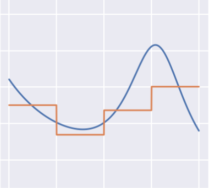
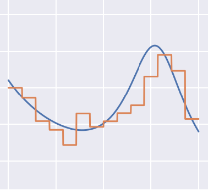
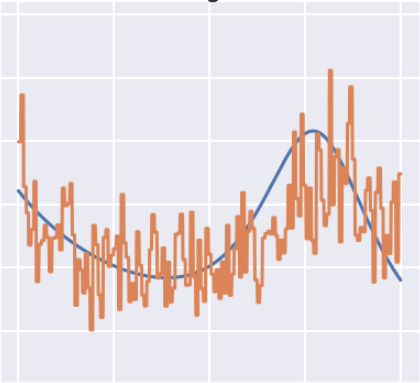
Figure 1: For a given segment, learned segmentized step function approximations (orange) of a true function (blue) which was used to generate a synthetic data-set. In the left - too few bins, bad approximation. In the middle - a balanced number of bins, moderate approximation. On the right - many bins, but approximation gets even worse due to a sparsity issue.

In this work, we propose a technique to improve the accuracy of FM variants by reducing the approximation gap without sparsity issues, while preserving training and inference speeds. Our technique is composed of encoding a numerical field using a vector of functions, which we refer to as basis functions, and a minor but significant modification to the computational graph of an FM variant. The idea of using basis functions is of course a standard practice with linear models, but combined with FMs it is surprisingly powerful, and radically differs from the same technique applied to linear models.

Indeed, we present an elementary lemmas showing that the resulting model learns a segmentized output function spanned by chosen basis, meaning that spanning coefficient depend on the values of the remaining fields. This is, of course, an essential property for recommendation systems, since indeed users with different demographic or contextual properties may behave differently. To the best of our knowledge, the idea of using arbitrary basis functions with FMs and the insights we present regarding the representation power of such a combination are new.

Based on the generic observation above, we offer the B-Spline basis [13, pp 87] defined on the unit interval on uniformly spaced break-points, composed onto a transformation that maps the feature to the unit interval. The number of break-points (knots) is a hyper-parameter. The strong approximation power of splines ensures that we do not need a large number of break-points, meaning that we can closely approximate the optimal segmentized functions, without introducing sparsity issues. Moreover, to make integration of our idea easier in a practical production-grade recommendation system easier, we present a technique to seamlessly integrate a model trained using our proposed scheme into an existing recommendation system that employs binning, albeit with a controllable reduction in accuracy.

To summarize, the main contributions of this work are: (a) Basis encoding We propose encoding numerical features using a vector of basis functions, and introducing a minor change to the computational graph of FM variants. . (b) Spanning properties We show that using our method, any model from a family that includes many popular FM variants, learns a segmentized function spanned by the basis of our choice, and inherits the approximation power of that basis. (c) B-Spline basis We justify the use of the B-Spline basis from both theoretical and practical aspects, and demonstrate their benefits via numerical evaluation. (d) Ease of integration into an existing system We show how to integrate a model trained by our method into an existing recommender system which currently employs numerical feature binning, to significantly reduce integration costs.

1.1 Related work

If we allow ourselves to drift away from the FM family, we can find a variety of papers on neural networks for tabular data [2, 3, 17, 22, 32, 37, 38, 20]. Neural networks have the potential to achieve high accuracy and can be incrementally trained on newly arriving data using transfer learning techniques. Additionally, due to the universal approximation theorem [21], neural networks are capable of representing a segmentized function from any numerical feature to a real number. However, the time required to train and make inferences using neural networks is significantly greater than that required for factorization machines. Even though some work has been done to alleviate this gap for neural networks by using various embedding techniques [16], they have not been able to outperform other model types. As a result, in various practical applications, FMs are preferred over NNs. For this reason, in this work we focus on FMs in our work, and specifically on decreasing a gap between the representation power of FMs and NNs without introducing a significant computational and conceptual complexity.

A very simple but related approach to ours was presented in [10]. The work uses neural networks and represents a numerical value $z$ as the triplet $(z,z^{2},\sqrt{z})$ in the input layer, which can be seen as a variant of our approach using a basis of three functions. Another approach which bears similarity to ours also comes from works which use deep learning [9, 17, 38, 18]. In these works, first-order splines are used in the input layer to represent continuity, and the representation power of a neural network compensates for the weak approximation power of first-order splines. Here we do the opposite - we use the stronger approximation power of higher-order splines to compensate for the weaker representation power of factorization machines.

The recent work [11] uses a technique which appears to resemble ours, but focuses on a different model family [19]. In contrast, our work a significantly broader theoretical and practical scope: it applies to a wide range of FM variants, includes handling of unbounded domains and interaction with categorical features, and reports A/B test results on a real-world ad recommendation system.

Finally, a work on tabular data cannot go without mentioning gradient boosted decision trees (GBDT) [8, 25, 33], which are known to achieve state of the art results [17, 36]. However, GBDT models aren’t useful in a variety of practical applications, primarily due to significantly slower inference speeds, namely, it is challenging and costly to use GBDT models to rank hundreds of thousands of items in a matter of milliseconds.

2 Formal problem statement

We consider tabular data-sets with $m$ fields, each can be either numerical or categorical. A row in the data-set $(z_{1},\dots z_{m})$, is encoded into a feature vector:

$$\mathbf{x}=\operatorname{\mathbf{enc}}(z_{1},\dots z_{m})\equiv\begin{bmatrix}\operatorname{\mathbf{enc}}_{1}(z_{1})\\ \vdots\\ \operatorname{\mathbf{enc}}_{m}(z_{m})\end{bmatrix},$$

where the $\operatorname{\mathbf{enc}}_{f}$ function encodes field $f$ into a vector, e.g. one-hot encoding of a single-valued categorical field. The vector $\mathbf{x}$ is then fed into a model. With a slight abuse of notation, we will denote by $\phi_{f}$ the model’s segmentized output, which is the output as a function of the value of a field $f$, assuming the remaining fields are some given constants. As in any supervised learning task, $\phi_{f}$ aims to approximate some unknown optimal segmentized function.

In the vast majority of cases, a numerical field $f$ is either encoded using a scalar transform $\operatorname{\mathbf{enc}}_{f}:\mathbb{R}\to\mathbb{R}$, or using binning - the numerical domain is partitioned into a finite set of intervals $\operatorname{\mathbf{enc}}_{f}(z_{f})$ is a one-hot encoding of the interval $z_{f}$ belongs to. Since for any $z_{f}\in[a_{i},a_{i+1})$ we have the same encoding, a deterministic model will produce the same output, and therefore $\phi_{f}$ is a step function.

Step functions are weak approximators in the sense that many cut-points are required to achieve good approximation accuracy. For example, Lipschitz-continuous functions can be approximated by a step function on $\ell$ intervals up to an error of only $O(\frac{1}{\ell})$ [13, pp 149]. Hence, with binning we need to strike an intricate balance between the theoretically-achievable approximation accuracy and our ability to achieve it because of sparsity issues, as illustrated in Figure 1. Note, that the above observation does not depend on weather the bins are chosen a-priori or learned. In this work we propose an alternative to binning, by encoding numerical features in a way that allows achieving more of the theoretical accuracy before sparsity issues take effect.

2.1 The factorization machine family

In this work we consider several model variants, which we refer to as the factorization machine family. The family includes celebrated factorization machine (FM) [34], the field-aware factorization machine (FFM) [24], the field-weighted factorization machine (FwFM) [29], and the field-matrixed factorization machine (FmFM) [39, 30], that generalized the former variants.

As a convention, we denote by $f_{i}$ the field which was used to encode the $i^{\text{th}}$ component of the feature vector $\mathbf{x}$, and denote arbitrary fields by $f,e$. We also denote by $\langle\mathbf{x},\mathbf{y}\rangle_{\mathbf{P}}=\mathbf{x}^{T}\mathbf{P}\mathbf{y}$ the “inner product” associated with some matrix $\mathbf{P}$. The FmFM model computes

$$\phi_{\mathrm{FmFM}}(\mathbf{x})=w_{0}+\langle\mathbf{x},\mathbf{w}\rangle+\sum_{i=1}^{n}\sum_{j=i+1}^{n}\langle x_{i}\mathbf{v}_{i},x_{j}\mathbf{v}_{j}\rangle_{\mathbf{M}_{f_{i},f_{j}}},$$ (1)

where $w_{0}\in\mathbb{R}$, $\mathbf{w}\in\mathbb{R}^{n}$, and $\mathbf{v}_{1}\in\mathbb{R}^{k_{1}}$, …, $\mathbf{v}_{n}\in\mathbb{R}^{k_{n}}$ are learned parameters, and the field-interaction matrices $\mathbf{M}_{f_{i},f_{j}}$ can be either learned, predefined, or have a special structure. Note, that this model family allows for different embedding dimension for each field, since the field interaction matrices do not have to be square.

It is easy to verify that all the aforementioned FM family member are special cases of FmFM. Indeed, with $\mathbf{M}_{e,f}=\mathbf{I}$ we obtain the regular FM [34]. Using $\mathbf{M}_{e,f}=\mathbf{P}_{e}^{T}\mathbf{P}_{f}$, where $\mathbf{P}_{f}$ is a matrix which extracts the components corresponding to the field $f$, we obtain the FFM [24], assuming embedding vector of each feature is concatenation of per-field interaction vectors. Finally, using $\mathbf{M}_{e,f}=s_{e,f}\mathbf{I}$ for some learned scalars $s_{e,f}$ the FwFM is obtained.

Since FmFM generalizes the entire family under consideration, we use equation (1) as the formalism to describe and prove properties which should hold for the entire family.

3 The basis function encoding approach

To describe our approach we need to introduce a slight modification to the FmFM computational graph described in Equation (1). Before feeding the vectors $x_{i}\mathbf{v}_{i}$ and scalars $x_{i}w_{i}$ into the factorization machine, we pass the vectors and, respectively, scalars belonging to each field through a linear reduction associated with that field. We consider two reductions: (a) the identity reduction, which just returns its input; and (b) a sum reduction, which sums up the $x_{i}\mathbf{v}_{i}$ and, respectively, the $x_{i}w_{i}$ of the corresponding field. Clearly, choosing the identity function for all fields reduces back to the regular FmFM model.

For a field $f$ that we designate as continuous numerical, we choose a set of functions $B_{1},\dots,B_{\ell}$, and encode the field as $\operatorname{\mathbf{enc}}_{f}(z)=(B_{1}(z),\dots,B_{\ell}(z))^{T}$ with a subsequent summing reduction. For the remaining fields, we use the identity reduction. The process for $x_{i}\mathbf{v}_{i}$ is depicted in Figure 2. Note, that each field can have its own basis, and in particular, the number of basis functions between fields may differ. For a formal description using matrix notation we refer the readers to Appendix A.1.

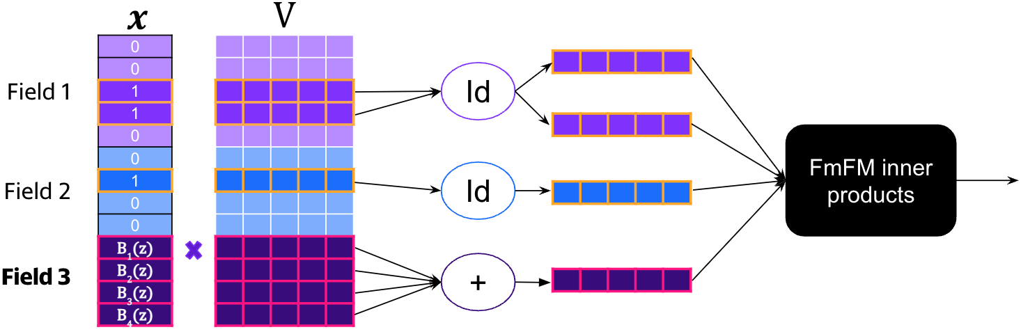
Figure 2: The computational graph with continuous numerical fields. Field 3 is a continuous numerical field whose value is $z$. The vectors $\mathbf{v}_{1},\dots,\mathbf{v}_{n}$ in the rows of $\mathbf{V}$ are multiplied by the input vector $\mathbf{x}$. Then, a reduction is applied to each field. Most fields have the identity (Id) reduction, whose output is identical to its input, whereas field 3 uses the sum reduction. The resulting vectors are then passed to the pairwise interaction module. An analogous process happens with the $\mathbf{w}$ vector.

3.1 Spanning properties

To show why our modeling choices improve the approximation power of the model, we prove two technical lemmas that establish a relationship between the basis of choice and the model’s output.

Lemma 1 (Spanning property).

Let $\operatorname{\mathbf{enc}}_{f}(z)=(B_{1}(z),\dotsm,B_{\ell}(z))^{T}$ be the encoding function associated with a continuous numerical field $f$, and suppose $\phi_{\mathrm{FmFM}}$ is computed according to Equation (1). Then, assuming the remaining field values are some given constants, there exist $\alpha_{1},\dots,\alpha_{\ell},\beta\in\mathbb{R}$, which depend on the values of the remaining fields and the model’s parameters but not on $z$, such that $\phi_{\mathrm{FmFM}}$ as a function of $z$ can be written as

$$\phi_{\mathrm{FmFM}}(z)=\sum_{i=1}^{\ell}\alpha_{i}B_{i}(z)+\beta.$$

An elementary formal proof can be found in Appendix A.2, but to convince the readers, we present an informal explanation. The vector stemming from a numerical field, after the summing reduction is a linear combination of the basis functions, while the remaining post-reduction vectors do no depend on $z$. Thus, when pairwise inner products are computed, we obtain a scalar which is a linear combination of the basis functions.

Another interesting result can be obtained by looking at $\phi_{\mathrm{FmFM}}$ as a function of two continuous numerical fields. It turns out that we obtain a function in the span of a tensor product of the two bases chosen for the two fields.

Lemma 2 (Pairwise spanning property).

Let $e,f$ be two continuous numerical fields. Suppose that $\operatorname{\mathbf{enc}}_{e}(z_{e})=(B_{1}(z_{e}),\dotsm B_{\ell}(z_{e}))^{T}$ and $\operatorname{\mathbf{enc}}_{f}(z_{f})=(C_{1}(z_{f}),\dotsm C_{\kappa}(z_{f}))^{T}$ be the encoding functions associate with the fields, and suppose $\phi_{\mathrm{FmFM}}$ is computed according to Equation (1). Define $B_{0}(z)=C_{0}(z)=1$. Then, assuming the remaining fields are kept constant, there exist $\alpha_{i,j},\beta\in\mathbb{R}$ for $i\in\{0,\dots,\ell\}$ and $j\in\{0,\dots,\kappa\}$, which depend on the values of the remaining fields and the model’s parameters but not on $z_{e},z_{f}$, such that $\phi_{\mathrm{FmFM}}$ as a function of $z_{e},z_{f}$ can be written as

$$\phi_{\mathrm{FmFM}}(z_{e},z_{f})=\sum_{i=0}^{\ell}\sum_{j=0}^{\kappa}\alpha_{i,j}B_{i}(z_{e})C_{j}(z_{f})+\beta.$$

The proof can be found in Appendix A.3. Note, that the model learns $O(\ell\cdot\kappa)$ segmentized coefficients without actually learning $O(\ell\cdot\kappa)$ parameters, but instead it learns only $O(\ell+\kappa)$ parameters in the form of $\ell+\kappa$ embedding vectors.

Essentially, the model learns an approximation of an optimal user behavior function for each continuous numerical field in the affine span of the chosen basis, or the tensor product basis in case of two fields. So it is natural to ask ourselves - which basis should we choose? Ideally, we should aim to choose a basis that is able to approximate functions well with a small number of basis elements, to keep training and inference efficient, and avoid over-fitting.

3.2 Cubic splines and the B-Spline basis

Spline functions [35] are piece-wise polynomial functions of degree $d$ with up to $d-1$ continuous derivatives defined on a set of consecutive sub-intervals of some interval $[a,b]$ defined a set of break-points $a=a_{0}<a_{1}<\dots<a_{\ell-d}=b$. The case of $d=3$ are known as cubic splines. These functions and variants are extensively used in computer graphics and computer aided design to accurately represent shapes of arbitrary complexity, due to their well-known strong approximation power, and efficient computational algorithms [12]. Here we concentrate on splines with uniformly spaced break points, and at this stage assume that the values of our numerical field lie in a compact interval. We discuss the more generic case in the following sub-section.

It well-known that spline functions can be written as weighted sums of the celebrated B-Spline basis [13, pp 87]. For brevity, we will not elaborate their explicit formula in this paper, but instead illustrate the basis in Figure 3, and point out that it’s available in a variety of standard scientific computing packages e.g. the scipy.interpolate.BSpline class of the SciPy package [41].

Figure 3: The cubic B-Spline basis of $\ell=8$ functions defined on $\ell-3=5$ uniformly spaced intervals broken by $0,1/5,2/5,\dots,1$. Any point in the interval is in the support of exactly four functions.

It is known [13, pp 149], that cubic splines can approximate an arbitrary function $g$ with $k\leq 4$ continuous derivatives up to an error bounded by $O(\|g^{(k)}\|_{\infty}/\ell^{k})$, where $g^{(k)}$ is the $k^{\text{th}}$ derivative of $g$. The spanning property (Lemma 1) ensures that the model’s segmentized outputs are splines spanned by the same basis, and therefore their power to approximate the optimal segmentized outputs. Therefore, assuming that the functions we aim to approximate are smooth enough and vary “slowly”, in the sense that their high-order $k^{\text{th}}$ derivatives are small, the approximation error goes down at the rate of $O(\tfrac{1}{\ell^{k}})$, whereas with binning the rate is $O(\tfrac{1}{\ell})$.

A direct consequence is that we can obtain a theoretically good approximation which is also achievable in practice, since we can be accurate with a small number of basis functions, and this significantly decreases the chances of sparsity issues. This is in contrast to binning, where high resolution binning is required to for a good theoretical approximation accuracy, but it may not be achievable in practice.

Yet another important property of the B-Spline basis is that at any point only four basis functions are non-zero, as is apparent in Figure 3. Thus, regardless of the number of basis functions we use, computing the model’s output remains efficient.

3.3 Numerical fields with arbitrary domain and distribution

Splines approximate functions on a compact interval, and the support of each basis function spans only a subset of the compact interval. Therefore, to learn a Spline function we require that the support of each basis function isn’t “starved” by the training data. Thus, fields with unbounded domains, or fields with highly skewed distributions, pose a challenge.

As a remedy, we propose first transforming a numerical $f$ using a function $T_{f}$ which has two objectives: (a) it maps the values to a compact interval, which we may assume w.l.o.g is the unit interval $[0,1]$, and (b) it ensures that there are no portions of the unit interval which are significantly “starved”. In practice, $T_{f}$ can be any function which roughly resembles the cumulative distribution function (CDF) of the field’s values. On small datasets we can use the QuantileTransform class from the Scikit-Learn package [7], but in a practical large-scale recommender system we can fit any textbook distribution, such as Normal or Student-T, to a sub-sample of the data. Note, that our method does not eliminate the need for data analysis, just simplifies it - instead of carefully tuning interval boundaries, we need to plot and fit a function to the distribution of the field’s values.

3.4 Integration into an existing system by simulating binning

Suppose we would like to obtain a model which employs binning of the field $f$ into a large number $N$ of intervals, e.g. $N=1000$. As we discussed in the Introduction, in most cases we cannot directly learn such a model because of sparsity issues. However, we can generate such a model from another model trained using our scheme to make initial integration easier.

The idea is best explained by referring, again, to Figure 2. For any value $z$ of the numerical field of our choice, the vector corresponding to that field after the reduction stage (field 3 in the figure) is a weighted sum of the field’s vectors, where the weights are $B_{i}(z)$. Thus, for any field value $z$ we can compute a corresponding embedding $\mathbf{p}(z)$. Given a set of $N$ intervals, we simply compute $N$ corresponding embedding vectors by evaluating $\mathbf{p}$ at the mid-point of each interval. The resulting model has an embedding vector for each bin, as we desired.

The choice of the set of interval break-points may vary between fields. For example, in many practical situations a geometric progression is applicable to fields with unbounded domains. Another natural choice is utilizing the transformation $T_{f}$ from the previous section, that resembles the data CDF, and using its inverse computed at uniformly spaced points as the bin boundaries, i.e., $\{T_{f}^{-1}(\tfrac{j}{N})\}_{j=0}^{N}$.

4 Evaluation

We divide this section into three parts. First, we use a synthetically generated data-set to show that our theory holds - the model learns segmentized output functions that resemble the ground truth. Then, we compare the accuracy obtained with binning versus splines on several data-sets. Finally, we report the results of a web-scale A/B test conducted on a major online advertising platform.

4.1 Learning artificially chosen functions

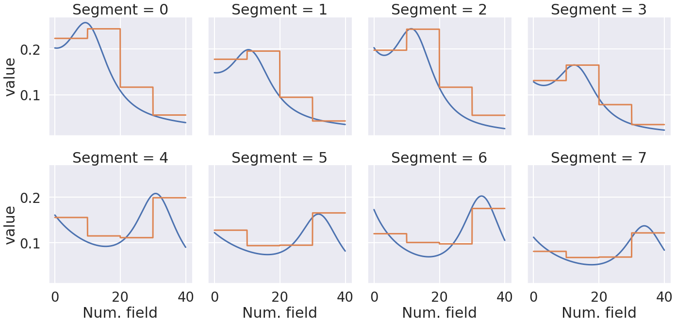
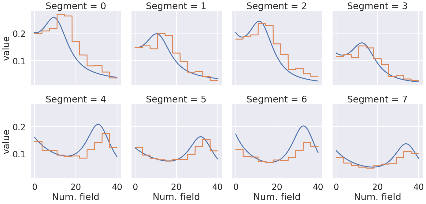
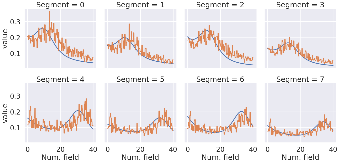
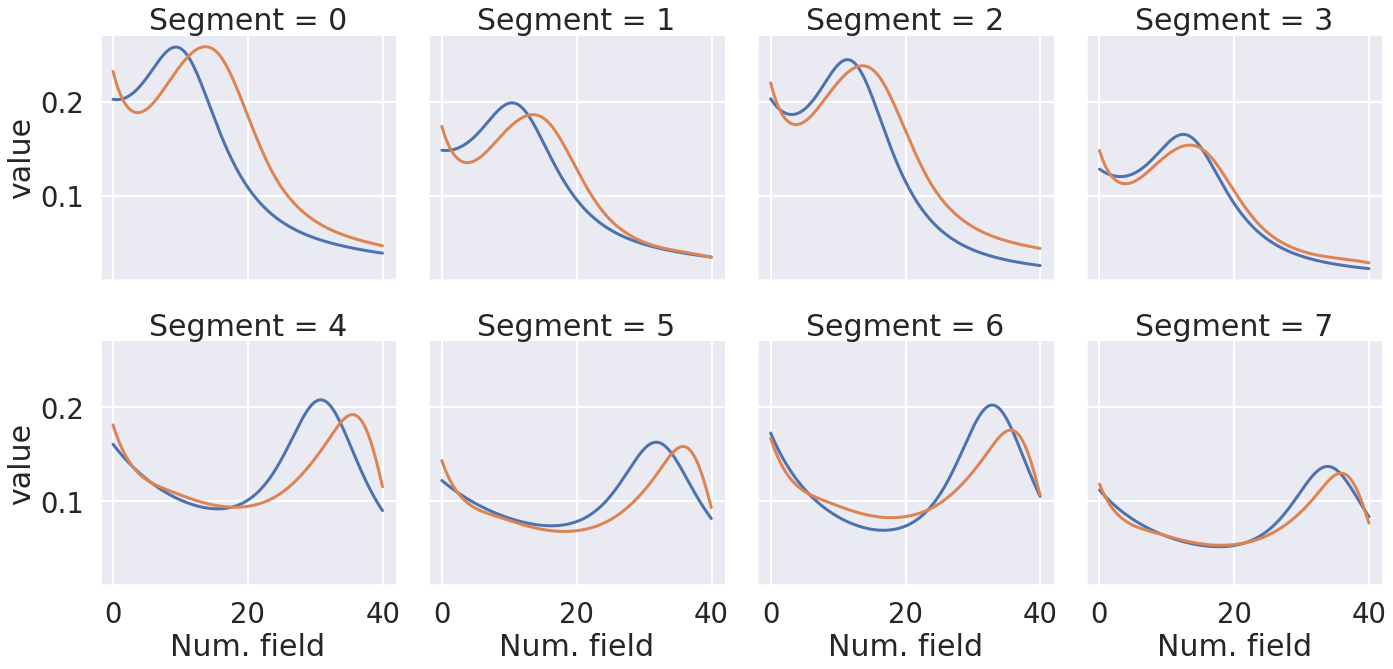
Figure 4: Results of segmentized approximations of four FFM models trained on our synthetic data-set, with 5, 12, and 120 bins, and splines with 6 break-points, down-left order. 5 bins have poor accuracy (test loss = 0.3474), 12 bins have a better accuracy (test loss = 0.3442), with 120 bins the accuracy worsens due to sparsity (test loss = 0.3478), and with splines we achieve best accuracy (0.3432).

We used a synthetic toy click-through rate prediction data-set with four fields, and zero-one labels (click / non-click). Naturally, the cross-entropy loss is used to train models on such tasks. We have three categorical fields each having two values each, and one numerical field in the range $[0,40]$. For each of the eight segment configurations defined by the categorical fields, we defined functions $p_{0},\dots,p_{7}$ (see Figure 4) describing the CTR as a function of the numerical field. Then, we generated a data-set of 25,000 rows, such that for each row $i$ we chose a segment configuration $s_{i}\in\{0,...,7\}$ of the categorical fields uniformly at random, the value of the numerical field $z_{i}\sim\operatorname{Beta-Binomial}(40,0.9,1.2)$, and a label $y_{i}\sim\operatorname{Bernoulli}(p_{s_{i}}(z_{i}))$.

We trained an FFM [24] provided by Yahoo [23] using the binary cross-entropy loss on the above data, both with binning of several resolutions and with splines defined on 6 sub-intervals. The numerical field was naïvely transformed to $[0,1]$ by simple normalization. We plotted the learned curve for every configuration in Figure 4. Indeed, low resolution binning approximates poorly, a higher resolution approximates better, and a too-high resolution cannot be learned because of sparsity. However, Splines defined on only six sub-intervals approximate the synthetic functions $\{p_{i}\}_{i=0}^{7}$ quite well.

Next, we compared the test cross-entropy loss on 75,000 samples generated in the same manner with for several numbers of intervals used for binning and cubic Splines. For each number of intervals we performed 15 experiments to neutralize the effect of random model initialization. As is apparent in Figure 5, Splines consistently outperform in this theoretical setting. The test loss obtained by both strategies diminishes if the number of intervals becomes too large, but the effect is much more significant in the binning solution.

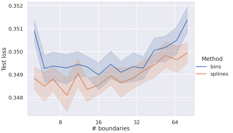
Figure 5: Comparison of the test cross-entropy loss obtained with Splines and bins. Both methods suffer from sparsity issues as the number of intervals grows, but Splines are able to utilize their approximation power with a small number of intervals, before sparsity takes effect.

4.2 External data-sets

We test our approach versus binning on several tabular data-sets: the california housing [28] , adult income [26], Higgs [4] (we use the 98K version from OpenML [40]), and song year prediction [5]. For the first two data-sets we used an FFM, whereas for the last two we used an FM, both provided by Yahoo [23], since an FFM is more expensive when there are many columns. We used Optuna [1] for hyperparameter tuning, e.g. step-size, batch-size, number of intervals, and embedding dimension, separately for each strategy. For binning, we also tuned the choice of uniform or quantile bins. In addition, 20% of the data was held out for validation, and regression targets were standardized. Finally, for the adult income data-set, 0 has a special meaning for two columns, and was treated as a categorical value. We ran 20 experiments with the tuned configurations to neutralize the effect of random initialization, and reported the mean and standard deviation of the metrics on the held-out set in Table 1, where it is apparent that our approach outperforms binning on these datasets.

	Cal. housing	Adult income	Higgs	Song year
# rows	20640	48842	98050	515345
# cat. fields	0	8	0	0
# num. fields	8	6	28	88
Metric type	RMSE	Cross-Entropy	Cross-Entropy	RMSE
Binning metric (std%)	0.4730 (0.36%)	0.2990 (0.47%)	0.5637 (0.22%)	0.9186 (0.4%)
Splines metric (std%)	0.4294 (0.57%)	0.2861 (0.28%)	0.5448 (0.12%)	0.8803 (0.2%)
Splines vs. binning	$-9.2\%$	$-4.3\%$	$-3.36\%$	$-4.16\%$

Table 1: Comparison of binning vs. splines. Standard deviations are reported as % of the mean.

4.3 A/B test results on an online advertising system

Here we report an online performance improvement measured using an A/B test, serving real traffic of a major online advertising platform. The platform applies a proprietary FM family click-through-rate (CTR) prediction model that is closely related FwFM [39]. The model, which provides CTR predictions for merchant catalogue-based ads, has a recency field that measures the time (in hours) passed since the user viewed a product at the advertiser’s site. We compared an implementation using our approach of continuous feature training and high-resolution binning during serving time described in Section 3.4 with a fine grained geometric progression of  200 bin break points, versus the “conventional” binned training and serving approach used in the production model at that time. The new model is only one of the rankers that participates in our ad auction. Therefore, a mis-prediction means the ad either unjustifiably wins or loses the auction, both leading to revenue losses.

We conducted an A/B test against the production model at that time, when our new model was serving $40\%$ of the traffic for over six days. The new model dramatically reduced the CTR prediction error, measured as $(\frac{\text{Average predicted CTR}}{\text{Measured CTR}}-1)$ on an hourly basis, from an average of $21\%$ in the baseline model, to an average of $8\%$ in the new model. The significant increase in accuracy has resulted in this model being adopted as the new production model.

5 Discussion

We presented an easy to implement approach for improving the accuracy of the factorization machine family whose input includes numerical features. Our scheme avoids increasing the number of model parameters and introducing over-fitting, by relying on the approximation power of cubic splines. This is explained by the spanning property together with the spline approximation theorems. Moreover, the discretization strategy described in Section 3.4 allows our idea to be integrated into an existing recommendation system without introducing major changes to the production code that utilizes the model to rank items.

It is easy to verify that our idea can be extended to factorization machine models of higher order [6].In particular, the spanning property in Lemma 1 still holds, and the pairwise spanning property in Lemma 2 becomes $q$-wise spanning property from machines of order $q$. However, to keep the paper focused and readable, we keep the analysis out of the scope of this paper.

With many advantages, our approach is not without limitations. We do not eliminate the need for data research, which is often required when working with tabular data, since the data still needs to be analyzed to fit a function that roughly resembles the empirical CDF. Feature engineering becomes somewhat easier, but some work still has to be done.

Finally, we would like to note that our approach may not be applicable to all kinds of numerical fields. For example, consider a product recommendation system with a field containing the price of a product. Usually higher prices mean a different category of products, leading to a possibly different trend of user preferences. In that case, the optimal segmentized output as a function of the product’s price is probably far from having small (higher order) derivatives, and thus cubic splines may perform poorly, and possibly even worse than simple binning.

Appendix A Proof of the spanning properties

First, we write the FmFM model using matrix notation. Then, we use the matrix notation to prove our Lemmas.

A.1 Formalization using linear algebra

To formalize our approach, we denote by $\mathbf{V}$ the matrix whose rows are the vectors $\mathbf{v}_{i}$, and decompose the FmFM formula (1) into three sub-formulas:

$$\mathbf{y} =\operatorname{diag}(\mathbf{x})\mathbf{w},$$

$$\mathbf{P} =\operatorname{diag}(\mathbf{x})\mathbf{V},$$

$$\phi_{\mathrm{FmFM}} =w_{0}+\langle\mathbf{1},\mathbf{y}\rangle+\sum_{i=1}^{n}\sum_{j=i+1}^{n}\langle\mathbf{p}_{i},\mathbf{p}_{j}\rangle_{M_{f_{i},f_{j}}},$$

where the $\operatorname{diag}(\cdot)$ operator creates a diagonal matrix with the argument on the diagonal, $\mathbf{1}$ is a vector whose components are all $1$, and $\mathbf{p}_{i}$ is the $i$th row of $\mathbf{P}$. Next, we associate each field $f$ with a field reduction matrix $\mathbf{R}_{f}$, concatenate them into one big block-diagonal reduction matrix. Note, that neither the block matrices $R_{f}$, nor the matrix $R$ have to be square.

$$\mathbf{R}=\begin{bmatrix}\mathbf{R}_{1}&\mathbf{0}&\dots&\mathbf{0}\\ \mathbf{0}&\mathbf{R}_{2}&\dots&\mathbf{0}\\ \vdots&\vdots&\ddots&\vdots\\ \mathbf{0}&\mathbf{0}&\dots&\mathbf{R}_{m}\end{bmatrix},$$

and assuming $\mathbf{R}$ has $\hat{n}$ rows, we modify the FmFM formula as:

$$\hat{\mathbf{y}} =\mathbf{R}\operatorname{diag}(\mathbf{x})\mathbf{w},$$ (2)

$$\hat{\mathbf{P}} =\mathbf{R}\operatorname{diag}(\mathbf{x})\mathbf{V},$$

$$\phi_{\mathrm{FmFM}} =w_{0}+\langle\mathbf{1},\hat{\mathbf{y}}\rangle+\sum_{i=1}^{\hat{n}}\sum_{j=i+1}^{\hat{n}}\langle\hat{\mathbf{p}}_{i},\hat{\mathbf{p}}_{j}\rangle_{M_{f_{i},f_{j}}}.$$

Setting $\mathbf{R}_{f}=\mathbf{I}$ for a field $f$ amounts to the identity reduction, whereas setting $\mathbf{R}_{f}=\mathbf{1}^{T}$, will cause the scalars $x_{i}w_{i}$ and the vectors $x_{i}\mathbf{v}_{i}$ to be summed up, resulting in the summing reduction. This matrix notation is useful for the study of the theoretical properties of our proposal, but in practice we will apply the field reductions manually, as efficiently as possible without matrix multiplication.

A.2 Proof of the spanning property (Lemma 1)

Proof.

Recall that we need to rewrite (2) as a function of $z$. For some vector $\mathbf{q}$, denote by $\mathbf{q}_{a:b}$ the sub-vector $(q_{a},\dots,q_{b})$. Assume w.l.o.g that $f=1$, and that field $1$ has the value $z$. By construction in (2), we have $\hat{y}_{1}=\sum_{i=1}^{\ell}w_{i}B_{i}(z)$, while the remaining components $\hat{\mathbf{y}}_{2:\hat{n}}$ do not depend on $z$. Thus, the we have

$$w_{0}+\langle\mathbf{1},\hat{\mathbf{y}}\rangle=\sum_{i=1}^{\ell}w_{i}B_{i}(z)+\underbrace{w_{0}+\langle\mathbf{1},\hat{\mathbf{y}}_{2:\hat{n}}\rangle}_{\beta_{1}}.$$ (3)

Moreover, by (2) we have that $\hat{\mathbf{p}}_{1}=\sum_{i=1}^{\ell}\mathbf{v}_{i}B_{i}(z)$, whereas the remaining rows $\hat{\mathbf{p}}_{2},\dots,\hat{\mathbf{p}}_{\hat{n}}$ do not depend on $z$. Thus,

$$\sum_{i=1}^{\hat{n}}\sum_{j=i+1}^{\hat{n}}\langle\hat{\mathbf{p}}_{i},\hat{\mathbf{p}}_{j}\rangle_{M_{f_{i},f_{j}}} =\sum_{j=2}^{\hat{n}}\langle\hat{\mathbf{p}}_{1},\hat{\mathbf{p}}_{j}\rangle_{M_{1,f_{j}}}+\underbrace{\sum_{i=2}^{\hat{n}}\sum_{j=i+1}^{\hat{n}}\langle\hat{\mathbf{p}}_{i},\hat{\mathbf{p}}_{j}\rangle_{M_{f_{i},f_{j}}}}_{\beta_{2}}$$ (4)

$$=\sum_{j=2}^{\hat{n}}\langle\sum_{i=1}^{\ell}\mathbf{v}_{i}B_{i}(z),\hat{\mathbf{p}}_{j}\rangle_{M_{1,f_{j}}}+\beta_{2}$$

$$=\sum_{i=1}^{\ell}\underbrace{\left(\sum_{j=2}^{\hat{n}}\langle\mathbf{v}_{i},\hat{\mathbf{p}}_{j}\rangle_{M_{1,f_{j}}}\right)}_{\tilde{\alpha}_{i}}B_{i}(z)+\beta_{2}$$

Combining Equations (3) and (4), we obtain

$$\phi_{\mathrm{FmFM}}(z)=\sum_{i=1}^{\ell}(w_{i}+\tilde{\alpha}_{i})B_{i}(z)+(\beta_{1}+\beta_{2}),$$

which is of the desired form. ∎

A.3 Proof of the pairwise spanning property (Lemma 2)

Proof.

Recall that we need to rewrite (2) as a function of $z_{e},z_{f}$, which are the values of the fields $e$ and $f$. Assume w.l.o.g that $e=1,f=2$. By construction in (2), we have $\hat{y}_{1}=\sum_{i=1}^{\ell}w_{i}B_{i}(z_{1})$, and $\hat{y}_{2}=\sum_{i=1}^{\kappa}w_{i}C_{i}(z_{2})$, while the remaining components $\hat{\mathbf{y}}_{3:\hat{n}}$ do not depend on $z$. Thus, the we have

$$w_{0}+\langle\mathbf{1},\hat{\mathbf{y}}\rangle=\sum_{i=1}^{\ell}w_{i}B_{i}(z_{1})+\sum_{i=1}^{\kappa}w_{i+\ell}C_{i}(z_{2})+\underbrace{w_{0}+\langle\mathbf{1},\hat{\mathbf{y}}_{3:\hat{n}}\rangle}_{\beta_{1}}$$ (5)

$$=\sum_{i=0}^{\ell}\sum_{j=0}^{\kappa}\hat{\alpha}_{i,j}B_{i}(z_{1})C_{j}(z_{2})+\beta_{1},$$

where $\hat{\alpha}_{i,0}=w_{i},\hat{\alpha}_{0,j}=w_{i+\ell}$ for all $i,j\geq 1$, for all other values of $i,j$ we set $\hat{\alpha}_{i,j}=0$.

Moreover, by (2) we have that $\hat{\mathbf{p}}_{1}=\sum_{i=1}^{\ell}\mathbf{v}_{i}B_{i}(z_{1})$ and $\hat{\mathbf{p}}_{2}=\sum_{i=1}^{\kappa}\mathbf{v}_{i}C_{i+\ell}(z_{2})$, whereas the remaining rows $\hat{\mathbf{p}}_{3},\dots,\hat{\mathbf{p}}_{\hat{n}}$ do not depend on $z_{1},z_{2}$. First, let us rewrite the interaction between $z_{1},z_{2}$ specifically:

$$\langle p_{1},p_{2}\rangle_{M_{1,2}}=\langle\sum_{i=1}^{\ell}\mathbf{v}_{i}B_{i}(z),\sum_{i=1}^{\kappa}\mathbf{v}_{i+\ell}C_{i}(z)\rangle_{M_{1,2}}=\sum_{i=1}^{\ell}\sum_{j=1}^{\kappa}\underbrace{\langle\mathbf{v}_{i},\mathbf{v}_{j+\ell}\rangle_{M_{1,2}}}_{\gamma_{i,j}}B_{i}(z_{1})C_{j}(z_{2})$$ (6)

By following similar logic to 4 one can obtain a similar expression when looking at the partial sums that include the interaction between $f$ (resp. $e$) and all other fields except $e$ (resp. $f$). Observe that the interaction between all other values does not depend on $z_{1},z_{2}$. Given all of this, we show how to rewrite the interaction as a function of $z_{1},z_{2}$:

$$\sum_{i=1}^{\hat{n}} \sum_{j=i+1}^{\hat{n}}\langle\hat{\mathbf{p}}_{i},\hat{\mathbf{p}}_{j}\rangle_{M_{f_{i},f_{j}}}$$ (7)

$$=\langle\hat{\mathbf{p}}_{1},\hat{\mathbf{p}}_{2}\rangle_{M_{1,2}}+\sum_{j=3}^{\hat{n}}\langle\hat{\mathbf{p}}_{1},\hat{\mathbf{p}}_{j}\rangle_{M_{1,f_{j}}}+\sum_{j=3}^{\hat{n}}\langle\hat{\mathbf{p}}_{2},\hat{\mathbf{p}}_{j}\rangle_{M_{2,f_{i}}}+\underbrace{\sum_{i=3}^{\hat{n}}\sum_{j=i+1}^{\hat{n}}\langle\hat{\mathbf{p}}_{i},\hat{\mathbf{p}}_{j}\rangle_{M_{f_{i},f_{j}}}}_{\beta_{2}}$$

$$=\sum_{i=1}^{\ell}\sum_{j=1}^{\kappa}\gamma_{i,j}B_{i}(z_{1})C_{j}(z_{2})+\sum_{i=1}^{\ell}\tilde{\alpha}_{i}B_{i}(z_{1})+\sum_{i=1}^{\kappa}\bar{\alpha}_{i}C_{i}(z_{2})+\beta_{2}$$

where $\tilde{\alpha}_{i},\bar{\alpha}_{i}$ are obtained similarly in equation 4’s final step.

∎

References

- [1] Takuya Akiba, Shotaro Sano, Toshihiko Yanase, Takeru Ohta, and Masanori Koyama. Optuna: A next-generation hyperparameter optimization framework. In Proceedings of the 25th ACM SIGKDD International Conference on Knowledge Discovery and Data Mining, 2019.
- [2] Sercan Ö. Arik and Tomas Pfister. Tabnet: Attentive interpretable tabular learning. Proceedings of the AAAI Conference on Artificial Intelligence, 35(8):6679–6687, May 2021.
- [3] Sarkhan Badirli, Xuanqing Liu, Zhengming Xing, Avradeep Bhowmik, Khoa Doan, and Sathiya S. Keerthi. Gradient boosting neural networks: Grownet, 2020.
- [4] Pierre Baldi, Peter Sadowski, and Daniel Whiteson. Searching for exotic particles in high-energy physics with deep learning. Nature communications, 5(1):4308, 2014.
- [5] Thierry Bertin-Mahieux, Daniel PW Ellis, Brian Whitman, and Paul Lamere. The million song dataset. 2011.
- [6] Mathieu Blondel, Akinori Fujino, Naonori Ueda, and Masakazu Ishihata. Higher-order factorization machines. In D. Lee, M. Sugiyama, U. Luxburg, I. Guyon, and R. Garnett, editors, Advances in Neural Information Processing Systems, volume 29. Curran Associates, Inc., 2016.
- [7] Lars Buitinck, Gilles Louppe, Mathieu Blondel, Fabian Pedregosa, Andreas Mueller, Olivier Grisel, Vlad Niculae, Peter Prettenhofer, Alexandre Gramfort, Jaques Grobler, Robert Layton, Jake VanderPlas, Arnaud Joly, Brian Holt, and Gaël Varoquaux. API design for machine learning software: experiences from the scikit-learn project. In ECML PKDD Workshop: Languages for Data Mining and Machine Learning, pages 108–122, 2013.
- [8] Tianqi Chen and Carlos Guestrin. Xgboost: A scalable tree boosting system. In Proceedings of the 22nd ACM SIGKDD International Conference on Knowledge Discovery and Data Mining, KDD ’16, page 785–794, New York, NY, USA, 2016. Association for Computing Machinery.
- [9] Yuan Cheng. Dynamic explicit embedding representation for numerical features in deep ctr prediction. In Proceedings of the 31st ACM International Conference on Information & Knowledge Management, pages 3888–3892, 2022.
- [10] Paul Covington, Jay Adams, and Emre Sargin. Deep neural networks for youtube recommendations. In Proceedings of the 10th ACM Conference on Recommender Systems, RecSys ’16, page 191–198, New York, NY, USA, 2016. Association for Computing Machinery.
- [11] Rügamer David. Additive higher-order factorization machines, 2022.
- [12] Carl de Boor. Subroutine package for calculating with b-splines. Technical report, Los Alamos National Lab.(LANL), Los Alamos, NM (United States), 1971.
- [13] Carl de Boor. A Practical Guide to Splines, volume 27 of Applied Mathematical Sciences. Springer-Verlag New York, 2001.
- [14] James Dougherty, Ron Kohavi, and Mehran Sahami. Supervised and unsupervised discretization of continuous features. In Armand Prieditis and Stuart Russell, editors, Machine Learning Proceedings 1995, pages 194–202. Morgan Kaufmann, San Francisco (CA), 1995.
- [15] João Gama and Carlos Pinto. Discretization from data streams: Applications to histograms and data mining. In Proceedings of the 2006 ACM Symposium on Applied Computing, SAC ’06, page 662–667, New York, NY, USA, 2006. Association for Computing Machinery.
- [16] Yury Gorishniy, Ivan Rubachev, and Artem Babenko. On embeddings for numerical features in tabular deep learning. In Advances in Neural Information Processing Systems, volume 35, pages 24991–25004, 2022.
- [17] Yury Gorishniy, Ivan Rubachev, Valentin Khrulkov, and Artem Babenko. Revisiting deep learning models for tabular data. In M. Ranzato, A. Beygelzimer, Y. Dauphin, P.S. Liang, and J. Wortman Vaughan, editors, Advances in Neural Information Processing Systems, volume 34, pages 18932–18943. Curran Associates, Inc., 2021.
- [18] Huifeng Guo, Bo Chen, Ruiming Tang, Weinan Zhang, Zhenguo Li, and Xiuqiang He. An embedding learning framework for numerical features in ctr prediction. In Proceedings of the 27th ACM SIGKDD Conference on Knowledge Discovery & Data Mining, pages 2910–2918, 2021.
- [19] Trevor J Hastie. Generalized additive models. In Statistical models in S, pages 249–307. Routledge, 2017.
- [20] Noah Hollmann, Samuel Müller, Katharina Eggensperger, and Frank Hutter. TabPFN: A transformer that solves small tabular classification problems in a second. In NeurIPS 2022 First Table Representation Workshop, 2022.
- [21] Kurt Hornik, Maxwell Stinchcombe, and Halbert White. Multilayer feedforward networks are universal approximators. Neural Networks, 2(5):359–366, 1989.
- [22] Xin Huang, Ashish Khetan, Milan Cvitkovic, and Zohar Karnin. Tabtransformer: Tabular data modeling using contextual embeddings, 2020.
- [23] Yahoo Inc. Fully-vectorized weighted field embedding bags for recommender systems. https://github.com/yahoo/weighted_fields_recsys, 2023. [Online; accessed 01-May-2023].
- [24] Yuchin Juan, Yong Zhuang, Wei-Sheng Chin, and Chih-Jen Lin. Field-aware factorization machines for ctr prediction. In Proceedings of the 10th ACM Conference on Recommender Systems, RecSys ’16, page 43–50, New York, NY, USA, 2016. Association for Computing Machinery.
- [25] Guolin Ke, Qi Meng, Thomas Finley, Taifeng Wang, Wei Chen, Weidong Ma, Qiwei Ye, and Tie-Yan Liu. Lightgbm: A highly efficient gradient boosting decision tree. In I. Guyon, U. Von Luxburg, S. Bengio, H. Wallach, R. Fergus, S. Vishwanathan, and R. Garnett, editors, Advances in Neural Information Processing Systems, volume 30. Curran Associates, Inc., 2017.
- [26] Ron Kohavi. Scaling up the accuracy of naive-bayes classifiers: A decision-tree hybrid. In Proceedings of the Second International Conference on Knowledge Discovery and Data Mining, KDD’96, page 202–207. AAAI Press, 1996.
- [27] Huan Liu, Farhad Hussain, Chew Lim Tan, and Manoranjan Dash. Discretization: An enabling technique. Data mining and knowledge discovery, 6:393–423, 2002.
- [28] R Kelley Pace and Ronald Barry. Sparse spatial autoregressions. Statistics & Probability Letters, 33(3):291–297, 1997.
- [29] Junwei Pan, Jian Xu, Alfonso Lobos Ruiz, Wenliang Zhao, Shengjun Pan, Yu Sun, and Quan Lu. Field-weighted factorization machines for click-through rate prediction in display advertising. In Proceedings of the 2018 World Wide Web Conference, WWW ’18, page 1349–1357, New York, NY, USA, 2018. Association for Computing Machinery.
- [30] Harshit Pande. Field-embedded factorization machines for click-through rate prediction, 2021.
- [31] Liu Peng, Wang Qing, and Gu Yujia. Study on comparison of discretization methods. In 2009 International Conference on Artificial Intelligence and Computational Intelligence, volume 4, pages 380–384, 2009.
- [32] Sergei Popov, Stanislav Morozov, and Artem Babenko. Neural oblivious decision ensembles for deep learning on tabular data. In International Conference on Learning Representations, 2020.
- [33] Liudmila Prokhorenkova, Gleb Gusev, Aleksandr Vorobev, Anna Veronika Dorogush, and Andrey Gulin. Catboost: unbiased boosting with categorical features. In S. Bengio, H. Wallach, H. Larochelle, K. Grauman, N. Cesa-Bianchi, and R. Garnett, editors, Advances in Neural Information Processing Systems, volume 31. Curran Associates, Inc., 2018.
- [34] Steffen Rendle. Factorization machines. In 2010 IEEE International Conference on Data Mining, pages 995–1000, 2010.
- [35] Isaac Jacob Schoenberg. Contributions to the problem of approximation of equidistant data by analytic functions. part b. on the problem of osculatory interpolation. a second class of analytic approximation formulae. Quarterly of Applied Mathematics, 4(2):112–141, 1946.
- [36] Ravid Shwartz-Ziv and Amitai Armon. Tabular data: Deep learning is not all you need. Information Fusion, 81:84–90, 2022.
- [37] Gowthami Somepalli, Avi Schwarzschild, Micah Goldblum, C. Bayan Bruss, and Tom Goldstein. SAINT: Improved neural networks for tabular data via row attention and contrastive pre-training. In NeurIPS 2022 First Table Representation Workshop, 2022.
- [38] Weiping Song, Chence Shi, Zhiping Xiao, Zhijian Duan, Yewen Xu, Ming Zhang, and Jian Tang. Autoint: Automatic feature interaction learning via self-attentive neural networks. In Proceedings of the 28th ACM International Conference on Information and Knowledge Management, CIKM ’19, page 1161–1170, New York, NY, USA, 2019. Association for Computing Machinery.
- [39] Yang Sun, Junwei Pan, Alex Zhang, and Aaron Flores. Fm2: Field-matrixed factorization machines for recommender systems. In Proceedings of the Web Conference 2021, WWW ’21, page 2828–2837, New York, NY, USA, 2021. Association for Computing Machinery.
- [40] Joaquin Vanschoren, Jan N Van Rijn, Bernd Bischl, and Luis Torgo. Openml: networked science in machine learning. ACM SIGKDD Explorations Newsletter, 15(2):49–60, 2014.
- [41] Pauli Virtanen, Ralf Gommers, Travis E. Oliphant, Matt Haberland, Tyler Reddy, David Cournapeau, Evgeni Burovski, Pearu Peterson, Warren Weckesser, Jonathan Bright, Stéfan J. van der Walt, Matthew Brett, Joshua Wilson, K. Jarrod Millman, Nikolay Mayorov, Andrew R. J. Nelson, Eric Jones, Robert Kern, Eric Larson, C J Carey, İlhan Polat, Yu Feng, Eric W. Moore, Jake VanderPlas, Denis Laxalde, Josef Perktold, Robert Cimrman, Ian Henriksen, E. A. Quintero, Charles R. Harris, Anne M. Archibald, Antônio H. Ribeiro, Fabian Pedregosa, Paul van Mulbregt, and SciPy 1.0 Contributors. SciPy 1.0: Fundamental Algorithms for Scientific Computing in Python. Nature Methods, 17:261–272, 2020.