RetICL: Sequential Retrieval of In-Context Examples with Reinforcement Learning

Abstract

Many recent developments in large language models focus on prompting them to perform specific tasks. One effective prompting method is in-context learning, where the model performs a (possibly new) generation/prediction task given one (or more) examples. Past work has shown that the choice of examples can make a large impact on task performance. However, finding good examples is not straightforward since the definition of a representative group of examples can vary greatly depending on the task. While there are many existing methods for selecting in-context examples, they generally score examples independently, ignoring the dependency between them and the order in which they are provided to the large language model. In this work, we propose Retrieval for In-Context Learning (RetICL), a learnable method for modeling and optimally selecting examples sequentially for in-context learning. We frame the problem of sequential example selection as a Markov decision process, design an example retriever model using an LSTM, and train it using proximal policy optimization (PPO). We validate RetICL on math problem solving datasets and show that it outperforms both heuristic and learnable baselines, and achieves state-of-the-art accuracy on the TabMWP dataset. We also use case studies to show that RetICL implicitly learns representations of math problem solving strategies.

RetICL: Sequential Retrieval of In-Context Examples with Reinforcement Learning

Alexander Scarlatos  and Andrew Lan University of Massachusetts Amherst {ajscarlatos,andrewlan}@cs.umass.edu

1 Introduction

With the rising prominence of pre-trained large language models (LLMs), prior work has focused on how to best utilize them for various natural language tasks. One of the most popular methods for doing so is prompt tuning, which deals with carefully selecting the natural language prompt that maximizes model performance Liu et al. (2021b). While there are many approaches to prompt tuning, a very successful one is in-context learning (ICL) Brown et al. (2020). In ICL, examples of a new task the LLM may not have been trained on before are included in the prompt to the LLM, enabing it to leverage patterns in these examples in a few-shot way. However, the choice of which examples the LLM sees for a particular task can significantly affect the model’s performance Zhao et al. (2021).

The primary goal of ICL example selection is to define a function that ranks a list of examples, where the rank measures how well those examples will elicit a desired response from an LLM when they are given in the prompt. We formalize this function as $\phi(x,e_{1},\ldots,e_{T})$, where $x$ is the input for the current task (or problem statement in a math setting) and $e_{1},\ldots,e_{T}$ is a list of $T$ examples drawn from a corpus $\mathcal{C}$. Most prior works simplify the definition of $\phi$ by assuming that examples are conditionally independent given $x$. This assumption allows the factorization $\phi(x,e_{1},\ldots,e_{T})=\prod_{t=1}^{T}\phi_{t}(x,e_{t})$, thus only having to rank one example at a time and allowing us to select an optimal set of examples by selecting the $T$ examples in the corpus with the highest values of $\phi_{t}(x,e_{t})$. However, this conditional independence assumption doesn’t always hold: there is likely significant interplay between the roles of different examples in deciding the output of LLMs. Some tasks benefit from example diversity Su et al. (2022), while others may benefit from combining specific information across examples. In these cases, simply selecting the top-$T$ ranked examples may neglect ones that are ranked lower on their own but are useful in conjunction with other examples. Additionally, top-$T$ selection ignores the order in which examples are provided, which can have an impact on performance Lu et al. (2021).

1.1 Contributions

In this work, we propose RetICL (Retrieval for In-Context Learning), a fully learnable method that sequentially retrieves ICL examples by conditioning on both the current problem and examples that have already been selected. We frame the problem of sequential example selection as a Markov decision process (MDP) and train an example retriever model using reinforcement learning. We construct the model using an LSTM, where hidden states act as latent representations of MDP states, and model the example ranking function using a bilinear transformation between the latent and corpus spaces, enabling efficient inference-time maximization of $\phi(x,e_{1},\ldots,e_{T})$. We additionally propose a novel confidence reward function, which uses the perplexity of the generated solution to help guide training. We validate RetICL on the math word problem solving datasets TabMWP and GSM8K where it outperforms both heuristic and learnable baselines. Additionally, RetICL achieves state-of-the-art accuracy on TabMWP, improving over the current best method by $8.20\%$ . Finally, we qualitatively analyze RetICL’s learned policies and find that RetICL is able to implicitly infer problem solving strategies from problem statements and examples.

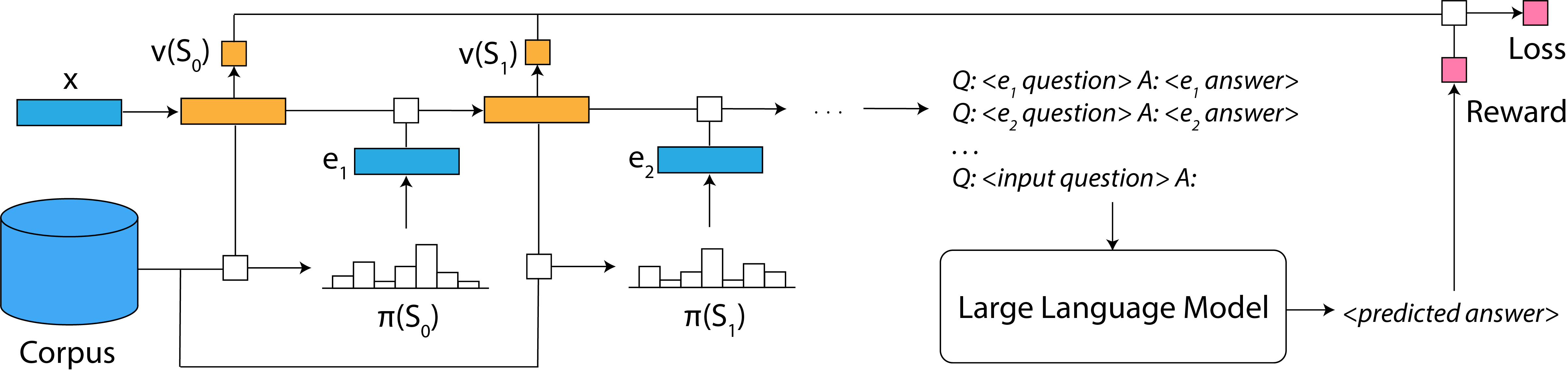
Figure 1: RetICL model architecture. Each latent state is constructed from the previous one and the current example. Examples are selected based on the bilinear transformation between the latent state and the corpus. After all examples are selected, the LLM is queried, the reward is calculated, and the loss is backpropagated into the model.

2 Related Work

In-Context Example Selection

When solving tasks in an ICL setting, it is common to either randomly select in-context examples Brown et al. (2020); Lewkowycz et al. (2022) or use a set of hand-crafted set of examples Hendrycks et al. (2021a); Wei et al. (2023). However, it is now well known that example selection and ordering for each input instance can have a large impact on downstream text generation performance Gao et al. (2020); Liu et al. (2021a); Zhao et al. (2021); Lu et al. (2021). Several prior works have found success in using heuristics to select examples Fu et al. (2022); Liu et al. (2021a); Su et al. (2022), while others have developed learnable example selection methods that use heuristics as training signals Rubin et al. (2021); Pitis et al. (2023). Our method differs from these in that our model’s training signal comes from per-problem performance in the target task. While we expect this distinction to help RetICL generalize to various tasks across domains, we focus only on math word problem solving in this work and leave exploration of other domains for future work. There are several other works that use reinforcement learning for ICL example selection. Lu et al. (2022) developed a policy gradient method for example selection, although their method does not include previously selected examples in the state, which is the key to our method. Zhang et al. (2022) used deep Q-Learning for policy learning, although their method only considers high-level summary information of previously selected examples, while our method uses their exact textual content.

Reinforcement Learning

Reinforcement learning (RL) is a machine learning paradigm where the goal is to learn a policy that maximizes the expected sum of rewards in an MDP. An MDP is a system defined by a temporal state, a set of potential actions, and a reward function Sutton and Barto (2018). While there are many RL algorithms, PPO Schulman et al. (2017), a policy gradient algorithm, has found significant success in natural language tasks, such as in its use for training ChatGPT OpenAI (2022) via reinforcement learning from human feedback Ziegler et al. (2019). However, RL algorithms can be notoriously challenging to train and often require a series of optimizations on top of the core algorithm. In this work, we implement PPO along with several modifications that are inspired by the observations listed in Andrychowicz et al. (2020), which we find to be necessary to improve training stability.

MWP Solving via In-Context Learning

Math word problem (MWP) solving is a difficult task due to limited mathematical reasoning abilities in LLMs Lewkowycz et al. (2022). As a result, various methods have been developed for MWP solving in ICL settings. A common technique known as chain-of-thought (CoT) prompting Wei et al. (2023) includes detailed reasoning steps for examples in the prompt, eliciting the LLM to also generate detailed reasoning steps and thus improve performance. Prior work also shows that providing in-context examples with more complex solutions can lead to improved performance Fu et al. (2022). Additionally, several inference-time methods have been developed to help LLMs with MWP solving. Using a calculator in the decoding pipeline Cobbe et al. (2021) can effectively reduce arithmetic errors in LLM output. Randomly sampling multiple solution outputs from the LLM and selecting the most common or consensus final answer, referred to as self-consistency Wang et al. (2023), also significantly improves accuracy. We note that in this work, we combine CoT prompting with our method but do not use inference-time techniques such as calculators or self-consistency, since they focus on a different aspect of the MWP solving pipeline and can be combined with our method.

3 Methodology

In this section, we detail how we frame ICL example selection as an MDP, how our example retriever model works, and how we train it using reinforcement learning. We show an overview of our methodology in Figure 1.

3.1 Example Selection as an MDP

We can view ICL example selection as a sequential decision making problem, where we select examples one at a time in such a way that we maximize our chances of achieving some goal when the examples are used as context. This goal is to maximize $r(\mathcal{M}(x,e_{1},\ldots,e_{T}),y)$, where $\mathcal{M}(\cdot)$ returns the generated output of an LLM given a prompt, $y$ is the label corresponding to $x$, and $r$ is a task-specific function that returns how good the generated output is. We note that in this setup, the order in which examples are selected matters since the order in which they are provided to $\mathcal{M}$ must be defined. We also note that while in this work we set $T$ to a constant, it can also be dynamically set during the decision-making process, which we leave for future work. With this framing, we can naturally define an MDP where the state at time step $t$ corresponds to both $x$ and the first $t$ examples that have been selected, and the action space is the set of potential candidates to be the next example. Formally,

$$S_{0}=x$$

$$S_{t}=x,e_{1},\ldots,e_{t}$$

$$A_{t}=e_{t+1}\in\mathcal{C}.$$

We now define the reward function for the MDP, which we break into two parts: a task-specific goal reward, and a supplementary confidence reward. We define the goal reward, $R^{G}$, simply as the output of $r$, as long as it can be formulated to return a scalar value. In the context of MWP solving, it is natural for $r$ to be binary, where it returns 1 when the generated solution results in a correct answer and returns -1 when the generated solution results in an incorrect answer, as is done in Lu et al. (2022). However, this reward function treats all correct solutions equally and all incorrect solutions equally, which can lead to suboptimal behavior since the model may have trouble distinguishing which correct solutions are better and which incorrect solutions are worse. To address this issue, we introduce the confidence reward, $R^{C}$, which we define as the inverse perplexity of the generated solution assigned by the LLM, normalized to the range $[-1,1]$. We hypothesize that when an LLM generates a correct solution with high probability (low perplexity), it is likely that the model “knew” how to solve the problem, rather than getting it correct by guessing or using unsound reasoning to arrive at a final answer. Additionally, we hypothesize that when an LLM generates an incorrect solution with high probability, it may have sound reasoning overall but contain a small error, such as an incorrect calculation, that leads to an incorrect final answer. While we find that the confidence reward is helpful in improving accuracy, we do not perform further analyses to validate our hypotheses, and leave such investigations for future work. We define the final reward function to be the average of $R^{G}$ and $R^{C}$ at the final time step and 0 at all prior time steps. Formally,

$$\hat{y}=\mathcal{M}(x,e_{1},\ldots,e_{T})$$

$$R^{G}=r(\hat{y},y)\overset{\text{MWP}}{=}2\cdot\mathbb{I}[g(\hat{y},y)]-1$$

$$R^{C}=2\cdot p_{\mathcal{M}}(\hat{y})^{\frac{1}{|\hat{y}|}}-1$$

$$R_{t}=\begin{cases}0.5R^{G}+0.5R^{C}&\text{if }t=T\\ 0&\text{otherwise},\end{cases}$$

where $\hat{y}$ is the generated solution, $g$ is a function that checks if two solutions have the same final answer, $\mathbb{I}$ is the indicator function, and $p_{\mathcal{M}}$ returns the probability assigned by the LLM. Next, we describe the retriever model which will define our policy, and how we train it using reinforcement learning.

3.2 Retriever Model

We now detail our model for example retrieval. At a high level, the model constructs a latent representation for each state $S_{t}$ in the MDP. The latent representation at $S_{t}$ is used to construct a probability distribution over all examples in the corpus, which we treat as the policy $\pi(S_{t},\cdot)$. We then use this policy to decide which example to select for state $S_{t+1}$ and the process continues sequentially.

We use an LSTM Hochreiter and Schmidhuber (1997) as the base model, where the hidden state $\mathbf{h}_{t}$ acts as the latent representation for $S_{t}$. We set the initial hidden state of the LSTM, $\mathbf{h}_{0}$, to be a vectorized embedding of the problem statement $x$, and set the input of the LSTM at time step $t$ to be a vectorized embedding of the example $e_{t}$. In this work, we construct these vectorized embeddings using a pre-trained S-BERT model Reimers and Gurevych (2019) and additionally provide learnable soft prompts Lester et al. (2021) to S-BERT to help align the embeddings with the current task. We found that fine-tuning the S-BERT parameters directly did not improve performance.

We use each hidden state $\mathbf{h}_{t}$ to produce two key outputs: the value function estimate at $S_{t}$ and the policy at $S_{t}$. The value function estimate, $\hat{v}(S_{t})$, is a learnable approximation of the expected sum of discounted rewards from $S_{t}$ till the final time step, and is required for variance reduction in policy gradient training. We produce this estimate using a simple linear transformation on top of $\mathbf{h}_{t}$. The policy, $\pi(S_{t},e)$, represents the probability of choosing $e$ to be the next example when we are in state $S_{t}$. We construct the policy by first producing an unnormalized activation value for each example in the corpus, $\phi(S_{t},e)$, and then use the softmax function to convert these activations into a probability distribution. We construct each $\phi(S_{t},e)$ by performing a learnable bilinear transformation between $\mathbf{h}_{t}$ and the vectorized embedding of $e$. We choose to model $\phi$ using a bilinear transformation for two reasons. First, the bilinear learns a mapping between the model’s latent space and the example embedding space, allowing generalization to examples not seen during training and also enabling some interpretability, as we will show later in this paper. Second, the bilinear enables efficient computation of the policy over a large corpus at inference time, as we will show later in this section. We formalize our model architecture as follows:

$$\mathbf{x}=\operatorname{S-BERT}(\mathbf{P}_{x},x)$$

$$\mathbf{e}=\operatorname{S-BERT}(\mathbf{P}_{e},e)$$

$$\mathbf{h}_{0}=\tanh(\mathbf{W}_{c}\mathbf{x}+\mathbf{b}_{c})$$

$$\mathbf{h}_{t>0}=\operatorname{LSTM}(\mathbf{e}_{1},\ldots,\mathbf{e}_{t};\mathbf{h}_{0})$$

$$\hat{v}(S_{t})=\mathbf{h}_{t}^{T}\mathbf{w}_{v}+b_{v}$$

$$\phi(S_{t},e)=\begin{cases}\mathbf{h}_{t}^{T}\mathbf{W}_{a}\mathbf{e}&\text{if }e\notin\{e_{1},\ldots,e_{t}\}\\ -\infty&\text{otherwise}\end{cases}$$

$$\pi(S_{t},e)=\frac{e^{\phi(S_{t},e)}}{\sum_{e^{\prime}\in\mathcal{C}}e^{\phi(S_{t},e^{\prime})}}$$

where $\mathbf{P}_{x}\in\mathbb{R}^{d_{p}\times d_{i}}$ and $\mathbf{P}_{e}\in\mathbb{R}^{d_{p}\times d_{i}}$ are learnable soft prompts, $\mathbf{W}_{c}\in\mathbb{R}^{d_{h}\times d_{e}}$ and $\mathbf{b}_{c}\in\mathbb{R}^{d_{h}}$ transform the problem statement embedding space into the latent space, $\mathbf{w}_{v}\in\mathbb{R}^{d_{h}}$ and $b_{v}\in\mathbb{R}$ produce the value function estimate from the latent space, $\mathbf{W}_{a}\in\mathbb{R}^{d_{h}\times d_{e}}$ performs the bilinear transformation between the latent space and example embedding space, $d_{p}$ is the soft prompt length, $d_{i}$ is the S-BERT input embedding size, $d_{e}$ is the S-BERT hidden size, and $d_{h}$ is the size of the latent space. We note that we set $\phi(S_{t},e)$ to $-\infty$ when $e$ has already been selected to avoid selecting the same example multiple times, which is in line with existing methods.

We now note that our formulation for $\phi$ allows efficient retrieval of the top-ranking example at each time step via maximum inner-product search (MIPS). We first note that $\phi(S_{t},e)$ is maximized by finding the example $e$ that maximizes the inner product $\langle\mathbf{h}_{t},\mathbf{W}_{a}\mathbf{e}\rangle$. We leverage this information by first pre-computing $\mathbf{W}_{a}\mathbf{e}$ for each example in the corpus and constructing a MIPS index over these vectors, using a library such as faiss Johnson et al. (2019). At inference time, we can now leverage algorithms that perform approximate MIPS in sublinear time, i.e., maximize $\phi(S_{t},e)$ without evaluating $\mathbf{h}_{t}^{T}\mathbf{W}_{a}\mathbf{e}$ for each example in the corpus. We note that we do not use MIPS in this work since the corpora we experiment on are sufficiently small such that evaluating $\mathbf{h}_{t}^{T}\mathbf{W}_{a}\mathbf{e}$ for each example in a corpus is relatively inexpensive. However, we expect that significant computational time can be saved with MIPS when evaluating on corpora at much larger scales.

3.3 Training and Inference

We train the retriever model using proximal policy optimization (PPO) Schulman et al. (2017) with generalized advantage estimation (GAE) Schulman et al. (2015) as our advantage function. We additionally use a reward discount of $\gamma=1$ since all episodes have fixed length and the reward is assigned only at the final time step. We train the value function estimator using mean squared error (MSE) with $R_{T}$ as the target at each time step and weigh the value function loss with a hyperparameter $c_{\text{VF}}$. We also encourage exploration by adding the negative entropy of the policy at each time step to the loss Ahmed et al. (2019), where we additionally weigh the entropy by a hyperparameter $c_{\text{E}}$ and normalize by $\frac{1}{\log(|\mathcal{C}|)}$ to account for training with different corpus sizes.

At train time, we select a batch of problems from the dataset, and then construct a sequence of examples for each problem by sequentially sampling from the policy, i.e., $e_{t+1}\sim\pi(S_{t},\cdot)$. When $T$ examples have been selected for each problem, we prompt the LLM with the examples and the current problem statement, calculate the reward from the LLM’s generations, average the PPO loss, value function loss, and entropy loss over the batch, and backpropagate through our model. At inference time, we greedily select examples from the policy, i.e., $e_{t+1}=\operatorname*{argmax}_{e\in\mathcal{C}}\pi(S_{t},e)$, since we find that greedy selection yields higher accuracy than sampling.

4 Experiments

In this section, we validate RetICL on math word problem (MWP) solving tasks and quantitatively compare its performance to several baselines. We also perform an ablation study and examine the effects of adjusting several parameters in order to determine which aspects of the methodology are working well and which may need improvement in future work.

4.1 Datasets

We validate RetICL on two MWP datasets that contain detailed solution steps: TabMWP Lu et al. (2022), where solving each problem requires extracting and reasoning with information from tables, and GSM8K Cobbe et al. (2021), where solving each problem requires multi-step mathematical reasoning and applying various arithmetic operations. We choose to use these datasets since the detailed solutions steps both allow CoT prompting and allow our model to interpret the solution steps when making example selections. To the best of our knowledge, these are the only two existing MWP datsets that contain detailed solutions steps, other than MATH Hendrycks et al. (2021b), which we found in preliminary investigations to be too difficult to achieve high accuracy on via ICL with the LLM we used. TabMWP has a pre-defined train/validation/test split of 23,059/7,686/7,686 problems, and GSM8K has a pre-defined train/test split of 7,473/1,319. We reserve 1,000 random problems from GSM8K’s train set for validation. For both datasets, we include the full step-by-step example solutions in the prompts and embeddings but evaluate the correctness of the solution based on only the final answer. We note that the official TabMWP evaluation code is flawed, since issues with regular expressions cause both false positives and false negatives when evaluating correctness on multiple choice problems. We instead use our own code to evaluate correctness on TabMWP, which we find fixes the issues with the original code.

4.2 Experimental Settings

We implement the PPO algorithm and the retriever model in PyTorch. We encode problem statements and examples using the all-distilroberta-v1 pre-trained S-BERT model Reimers and Gurevych (2019), take the normalized mean-pooled final layer outputs as the embeddings, and use a soft prompt length of 20. We use OpenAI’s code-davinci-002 Codex model Chen et al. (2021) as the LLM with greedy decoding and set the maximum number of generated tokens to 400. We use Codex since we found it to be more accurate than open-source models and text-davinci-003 on our tasks, to have better ICL prompting behavior than gpt-3.5-turbo on our tasks, and the API is free. We set the LSTM’s hidden size to 800, PPO’s $\epsilon$ to 0.1, GAE’s $\lambda$ to 0.9, and $c_{\text{VF}}$ to 0.5. We set $c_{\text{E}}$ to 0.05 for TabMWP and $c_{\text{E}}$ to 0.1 for GSM8K, where different values are necessary since we find that our method performs differently across datasets and that $c_{\text{E}}$ has a large impact on training stability. We use orthogonal initialization Hu et al. (2020) for all weight parameters, initialize all bias parameters to 0, and initialize soft prompts using a standard normal distribution. We train using the AdamW optimizer for 50 epochs with a learning rate of 0.001, a weight decay of 0.01, and a batch size of 20. We additionally apply gradient norm clipping on all parameters using a value of 2, which we find is critical to avoid spikes in training losses.

For each dataset, we randomly select 5,000 problems from the training set as our problems to train on, since we find that this number achieves a good balance between high accuracy and minimizing training time. We randomly select an additional 200 problems from the training set to use as the corpus of examples. While it is possible to use a larger corpus, e.g., all remaining problems in the training set, we find that training on a smaller corpus results in higher accuracy and that 200 works well in practice. We randomly select 500 problems from the validation set to evaluate performance on after each epoch. For validation and testing, we use the entire training set as the corpus, since we find that having access to as many examples as possible at inference time generally increases accuracy. We save the model at the epoch with the highest accuracy on the validation set for evaluation on the test set. We set the number of in-context examples to $T=2$ for all experiments, since this is the minimal number of examples required to evaluate the impact of selecting examples sequentially. We note that while modifying $T$ can have an impact on performance for both RetICL and baselines, we find that using a constant across methods provides a fair comparison of performance, and we leave exploration of this parameter for future work.

4.3 Baselines

We compare RetICL to three baseline in-context example selection methods: random selection, similarity-based kNN selection Liu et al. (2021a), and PromptPG Lu et al. (2022). We also perform exhaustive evaluation to serve as an approximate upper bound to the example selection methods.

Random

With random selection, for each problem, we randomly sample $T$ unique examples from the corpus for the ICL prompt. We evaluate random selection on 3 different random seeds and report the average accuracy across all 3 runs.

kNN

With kNN selection Liu et al. (2021a), for each problem, we select the $T$ examples with the most similar problem statements from the corpus and use those for the ICL prompt. We evaluate similarity by minimizing the Euclidean distance between the S-BERT embeddings of the problem statements using the same pre-trained S-BERT model as RetICL.

PromptPG

With PromptPG Lu et al. (2022), for each problem, a learned scoring function is evaluated on each individual example in the corpus, and the top $T$ scoring examples are selected for the ICL prompt. PromptPG is a similar method to RetICL in that it uses a policy gradient method to learn an ICL example scoring function. However, there are many key differences between their method and ours: they do not include previously selected examples in the state, their reward function only considers correctness of the final answer, they encode text using BERT instead of S-BERT and do not use fine-tuning or soft prompting, they use REINFORCE instead of PPO, they do not use entropy to boost exploration, they use a much smaller training size of 160, and they use corpus size of 20 for both training and inference. We evaluate PromptPG’s performance by running their code with modifications to match our prompting style and use our fixed evaluation code for fair comparison.

Exhaustive

With exhaustive evaluation, for each problem, we construct a one-shot ICL prompt for each example in the corpus, and consider the current problem to be solved if a correct solution is generated from any of the prompts. We use one-shot prompts instead of few-shot prompts to reduce the search space. Additionally, we restrict the corpus size to 100 and only evaluate on the pre-defined 1,000-sample subset of the test set for TabMWP to reduce computation time.

4.4 Results

Table 1 shows the performance of all methods on both datasets. We see that RetICL performs the best among non-exhaustive methods on both datasets, on par with kNN on TabMWP and significantly better on GSM8K. We also see that kNN is much better than Random on TabMWP but is only slightly better than Random on GSM8K. However, after investigating the dataset, we conclude that the high performance of kNN on TabMWP is likely due to the presence of many problems in the dataset with very high similarity. For example, many problems will have exactly the same question text other than a few numbers or names changed, making it easy for the LLM to generate a correct solution given a highly similar example. On the contrary, GSM8K does not tend to contain problems that are almost identical, which makes kNN ineffective since problems with high textual similarity may not have similar solution strategies.

Perhaps surprisingly, we see that PromptPG is only slightly better than Random on TabMWP and performs on par with Random on GSM8K. While these results contradict the trends reported in Lu et al. (2022), we believe the discrepancy is mostly due to using the fixed evaluation code. We believe that PromptPG’s relatively low performance also highlights the challenges of solving the ICL example selection problem using RL; many of the optimizations we implemented are required to achieve high performance in practice.

Additionally, we see that the Exhaustive method achieves almost perfect accuracy on both datasets. We find this surprising, especially due to the fact that Exhaustive only uses a single ICL example and has access to a smaller corpus. This result implies that there is significant room for growth in ICL example selection methods and also implies that one-shot ICL has the potential to be an extremely powerful inference method as long as the example corpus is informative, even for challenging text generation tasks.

Method	TabMWP	GSM8K
Exhaustive	98.20	97.95
Random	72.20	57.19
PromptPG${}_{\text{\cite[cite]{\@@bibref{Authors Phrase1YearPhrase2}{tab-mwp}{\@@citephrase{(}}{\@@citephrase{)}}}}}$	73.43	56.94
kNN${}_{\text{\cite[cite]{\@@bibref{Authors Phrase1YearPhrase2}{similarity}{\@@citephrase{(}}{\@@citephrase{)}}}}}$	88.49	59.21
RetICL	88.51	66.11

Table 1: Test set accuracy for RetICL and baselines.

In order to determine how well RetICL can generalize to low-resource settings, we examine the effect of reducing the number of available examples at test time. We evaluate RetICL and kNN on both datasets where 0.1%, 1%, 10%, and 100% of all examples are available as candidates, and show our results in Figure 2. Additionally, in order to more clearly demonstrate the generalizability of the methods, we show the relative accuracy compared to RetICL’s accuracy when the full corpus is available. For TabMWP, we evaluate on the pre-defined 1000-sample subset of the test set. We first observe that even with 0.1% of examples available, both methods still retain a large portion of their performance, which implies that both methods are still viable in low resource settings. We also note that RetICL still outperforms or ties kNN on all corpus sizes, implying that RetICL is still the preferred method across corpus sizes. We note that the relative drop in performance is greater for TabMWP than GSM8K, likely because the TabMWP corpus loses many examples that have high similarity to the test problems, whereas GSM8K doesn’t have such high similarity between problems. Finally, we note that in some cases a smaller corpus leads to higher relative performance. We believe that the peak in performance for kNN on GSM8K at 1% implies that kNN is a poor heuristic for this dataset, since the early peak means that examples with higher similarity can result in less accuracy. We note that RetICL is slightly higher at 10% than 100% on TabMWP, implying that the policy is not perfectly tuned, since the peak means that some examples that are preferred by the policy can lead to lower accuracy.

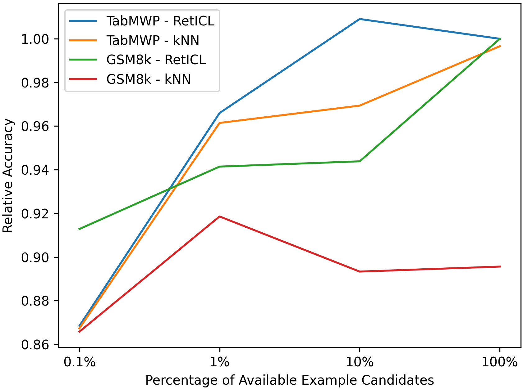
Figure 2: Change in relative accuracy as number of available example candidates increases.

4.5 Ablation study

Ablation	TabMWP		GSM8K
	Acc.	Ex.	Acc.	Ex.
None	88.20	197	66.11	97
$\text{T}_{\text{1k}}$	87.20	115	65.96	34
$\text{T}_{\text{1k}}$, Conf. Rew.	84.40	64	64.67	20
$\text{T}_{\text{1k}}$, LSTM	88.40	113	63.91	38
$\text{T}_{\text{1k}}$, Ent.	83.00	26	62.77	6
$\text{T}_{\text{1k}}$, SP	86.50	131	66.26	3
$\text{T}_{\text{1k}}$, SP, $\text{TC}_{20}$	84.20	81	61.87	58
$\text{T}_{\text{1k}}$, SP, $\text{TC}_{\text{all}}$	85.40	99	65.88	58

Table 2: Ablation study, measuring accuracy and number of examples used on both datasets.

We now examine the impact of various modeling and algorithmic choices via an ablation study. We train on 1,000 problems instead of 5,000 for all ablations for faster experimentation, and denote this reduced training size with $\textbf{T}_{\textbf{1k}}$. We experiment with the following adjustments:

• Conf. Rew.: We no longer use the confidence reward, $R^{C}$, and instead only use the goal reward, $R^{G}$.

• LSTM: We no longer condition on previously selected examples by removing the LSTM architecture and instead set the latent state for all time steps to be $\mathbf{h}_{0}$.

• Ent.: We no longer include an entropy term in the loss function.

• SP: We no longer provide learnable soft prompts to the S-BERT encoder. We note that this change significantly reduces the memory footprint since soft prompt tuning requires storing copies of partial gradients over all S-BERT parameters for each candidate example.

• $\textbf{TC}_{\textbf{20}}$ and $\textbf{TC}_{\textbf{all}}$: We vary the size of the corpus at train time, using a corpus with 20 problems from the training set and all remaining problems from the training set, respectively. We also apply the SP ablation for the TC ablations since otherwise the partial gradients over the S-BERT parameters will cause the system to run out of memory for $\text{TC}_{\text{all}}$.

Table 2 shows the results of the ablation study. We list both accuracy as well as the number of unique examples selected at inference time to examine the impact of each ablation on the diversity in the selected examples. For TabMWP, we evaluate on the pre-defined 1,000-sample subset of the test set.

We see that using 1,000 training problems only slightly reduces accuracy, although it significantly reduces example diversity. We also see that removing the confidence reward and the entropy loss significantly reduce accuracy and example diversity, implying that these modifications are key optimizations for training. Next, we see that removing the LSTM slightly improves accuracy for TabMWP but significantly drops accuracy for GSM8K, and for both datasets does not significantly impact example diversity. To explain this discrepancy, we find that for TabMWP, there are several cases where the non-LSTM model selects examples that are more relevant to the current problem compared to the LSTM model, implying that the LSTM model may have more trouble converging on a good policy and may require additional optimizations to fix this issue. Next, we see that removing soft prompting slightly drops accuracy for TabMWP but slightly improves accuracy and significantly reduces example diversity for GSM8K. We note that the training run for SP for GSM8K peaked in validation accuracy at an early epoch, so it is possible that the selected model for this run was in a local optimum that happened to have slightly better performance. Next, we see that only using 20 candidate examples at train time significantly hurts accuracy across datasets, although perhaps surprisingly, increases example diversity for GSM8K. Finally, we see that using all available examples as candidates during training hurts accuracy on both datasets. This drop in performance may be due to slower convergence on an optimal policy since the policy needs to explore a huge search space. We note that Lu et al. (2022) also observe that increasing the corpus size at train time does not necessary increase accuracy.

5 Qualitative Analysis

We now present several qualitative analyses in order to interpret RetICL’s example selection policy. Our goal in these analyses is to determine what features RetICL focuses on in individual examples, as well as what strategy RetICL uses to select an entire sequence of examples. We investigate these strategies by first visualizing learned latent example embeddings and then analyzing trends in per-problem example selections.

5.1 Latent Space Analysis

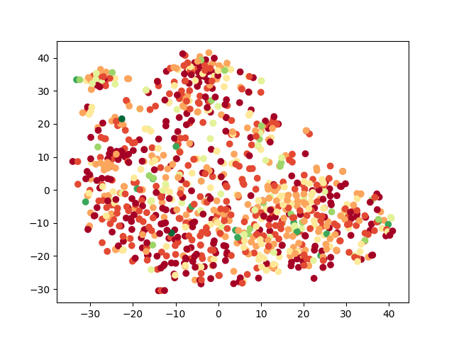
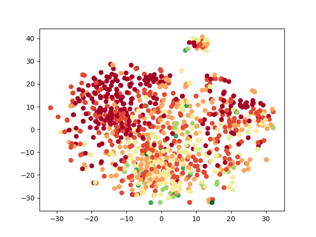
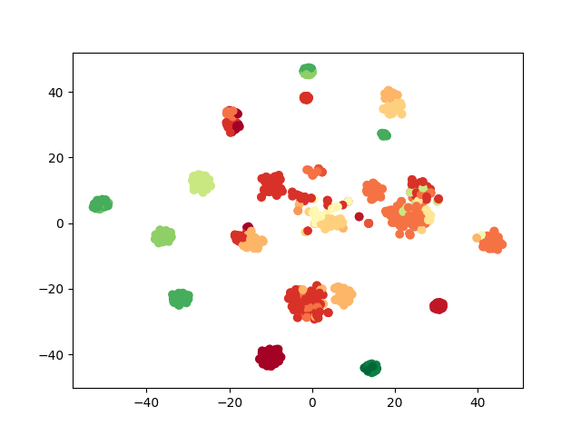
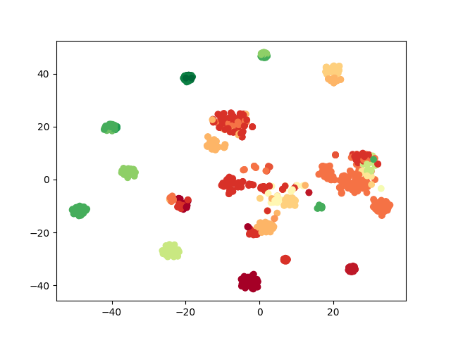
Figure 3: Example embedding visualizations. From left to right, top to bottom, GSM8K pre-trained embeddings, GSM8K RetICL embeddings, TabMWP pre-trained embeddings, and TabMWP RetICL embeddings.

In order to identify features in the selected examples that are being emphasized by RetICL, we perform a visual analysis of the example embeddings in the model’s latent space. Specifically, we transform each example embedding $\mathbf{e}$ into the model’s latent space using the right half of the bilinear from the $\phi$ function, i.e., $\mathbf{W}_{a}\mathbf{e}$. We note that because maximizing $\phi(S_{t},e)$ is equivalent to maximizing $\langle\mathbf{h}_{t},\mathbf{W}_{a}\mathbf{e}\rangle$, the most likely example to select at $S_{t}$ is the example where $\mathbf{W}_{a}\mathbf{e}$ is closest to $\mathbf{h}_{t}$ in the latent space. We can thus infer that examples that are close in the latent space have similar likelihood of being selected by the policy, which enables us to manually examine the policy’s rankings by examining patterns in local regions of latent example embeddings.

For both TabMWP and GSM8K, we randomly select 1,000 examples from the example corpus and then apply t-SNE Van der Maaten and Hinton (2008) to reduce their embeddings to 2 dimensions for visualization. Additionally, for the same sets of examples, we also visualize their pre-trained S-BERT embeddings in the same way, in order to demonstrate how inter-example similarities change after RetICL training. We color points based on the number of steps in an example’s solution, with red being the least, green being the most, and yellow being in the middle.

Figure 3 shows these visualizations. For GSM8K, we see that RetICL groups examples based on the number of solution steps, whereas the pre-trained S-BERT embeddings do not. This observation implies that the number of solution steps is an important factor in example selection, and confirms findings from prior work that solution complexity impacts generation performance Fu et al. (2022). We also see that clusters in the RetICL embeddings have been somewhat merged together from the pre-trained embeddings. This result can be interpreted by observing the pre-trained embeddings to be primarily clustered based on topic, e.g., problems about money and problems about time belong to separate clusters, since S-BERT embeddings reflect the semantic content of the examples. While local neighbors in the RetICL embedding space also tend to have similar topics, the clusters are less well-separated, which implies that both topic and the solution strategy, which is partly reflected in the length of solution steps, are used for example selection by RetICL.

For TabMWP, we see that the space looks very different from GSM8K, with many separate clusters being present in both the RetICL and pre-trained spaces, primarily based on the problem’s template. For example, there is one cluster for asking yes/no questions about schedules, one for asking if someone has enough money to buy something, and one for asking what the mean of a set of numbers is. Since RetICL retains these clusters, we can infer that an example’s template is key to example selection. This observation is also validated by kNN’s high performance on this dataset, since the most semantically similar problems are always from the same cluster. While there are not many differences between the RetICL and pre-trained S-BERT embedding spaces, we observe that RetICL has pulled several clusters closer together. For example, it partially merges together problems that require finding the largest value and problems that require finding the smallest value from a set. This observation suggests that problems across the merged template clusters can be used interchangeably as examples, since their problems tend to have similar reasoning strategies.

5.2 Per-Problem Example Selection

We now examine example selections at the per-problem level in order to gain further insight into RetICL’s learned example selection policy.

Table 3 shows the in-context examples selected to help solve a representative example problem from the GSM8K dataset. We see that RetICL tends to select examples that share some unique high-level features with the input problem. Examples of such features are subtracting from a total value, adding up monetary values over some period of time, and defining some variables to be proportional to other variables. We note that each problem in the dataset exhibits several such features, so RetICL has to implicitly decide which particular features are most important for the current problem and which examples most represent those features. We also see that RetICL tends to select examples with solutions that are relatively long and have substantial verbal reasoning. While RetICL’s selection strategy works well in many cases, there are several common scenarios where it fails. First, the LLM can exhibit misconceptions when it lacks an example to provide context, such as misinterpreting the meaning of a “discount” when not explicitly instructed. Second, the LLM can try to follow the examples too closely and use reasoning that does not necessarily apply to the current problem. These errors indicate that RetICL’s policy could be improved by selecting based on a broader and more targeted set of features. However, we note that many of the incorrect solutions do not appear to be due to poor example selection, since they contain simple errors such as incorrect arithmetic or switching the roles of variables in the problem. We believe these errors are due to limitations of the LLM and are a likely source of noise in the training signal, making it harder to find an optimal policy. We note that such errors can be fixed by using a calculator, self-consistency, or external computation engines Wolfram (2023), and we leave integration of such methods into RetICL for future work.

Table 4 shows the in-context examples selected to help solve a representative example problem from the TabMWP dataset. We see that RetICL’s selections tend to follow a surprising pattern: the first selected example is seemingly unrelated to the current problem, while the second selected example has similar reasoning steps to the current problem. This strategy has several implications. First, it suggests that RetICL can infer reasoning steps from the current problem and select examples based on this information. Second, it shows that there may be a benefit to a diverse set of examples in the prompt, possibly because an unrelated first example prevents overfitting to example solutions, or because there is some subtle benefit to seeing different kinds of calculations earlier in the context. We note that the incorrect solutions tend to be caused by either cases where RetICL diverges from the previously described strategy and selects an unrelated second example, or selects a second example that is similar to the current problem but requires a slightly different reasoning strategy. These failure cases imply that RetICL could benefit from training improvements to make its policy more consistent and stable, as well as architectural improvements of the model to be more accurate in inferring reasoning strategy from problem statement.

6 Conclusion

In this work, we proposed RetICL, a method for sequential in-context example selection that, unlike existing methods that select all examples independently, takes previously selected examples into account. We framed the problem of example selection as a Markov decision process and developed a novel reward function, an example retriever model, and ways to train the model. We demonstrated that RetICL learns an effective strategy for example selection and outperforms baselines on the task of math word problem solving. There are many avenues for future work. First, since we only validated RetICL for math problem solving, we can explore its usage in other natural language generation tasks to see if it can be used a generic method for selecting ICL examples. Second, we can explore other architectural modifications that could further improve the retriever model, such as using a Transformer instead of an LSTM. Third, since we used a fixed number of examples, we can extend RetICL to let it learn how many examples are needed. Fourth, we can explore whether RetICL can be applied to real-world educational settings, e.g., selecting worked examples to help students solve practice problems.

Limitations

We note that there are several practical limitations to our method. First, we note that RetICL can be expensive and time-consuming to train, with each of our main training runs requiring up to 250,000 LLM inferences. This high number of inferences makes training on paid models prohibitively expensive; for example, it could cost up to approximately $2,500 to train on OpenAI’s text-davinci models. Additionally, newer OpenAI models, such as gpt-3.5-turbo and gpt-4, do not return likelihood information on generated text, making the confidence reward impossible to use for these models.

Ethical Considerations

We first note that the high number of inferences required to train RetICL give the method an outsized cost in terms of energy usage; however, we note that the method has a relatively low cost at inference time given its low number of parameters and potential for optimization with MIPS. Additionally, we note that because RetICL uses a black-box LLM reward signal, its example selections are not guaranteed to be interpretable by humans. Finally, because we only examine the math problem solving domain, we did not perform any analysis of bias in RetICL’s selections. However, it is possible that RetICL could reflect biases in the LLM it is being trained on. As such, we recommend an analysis of bias in future works that use RetICL in sensitive settings such as student-facing educational tools.

Appendix A Examples

Problem
Marcus is half of Leo’s age and five years younger than Deanna. Deanna is 26. How old is Leo?
Gold Solution
Marcus is 26 - 5 = 21 years old. Thus, Leo is 21 * 2 = 42 years old. Final Answer: 42
RetICL	kNN
Selected Examples
Problem: Katy, Wendi, and Carrie went to a bread-making party. Katy brought three 5-pound bags of flour. Wendi brought twice as much flour as Katy, but Carrie brought 5 pounds less than the amount of flour Wendi brought. How much more flour, in ounces, did Carrie bring than Katy? Solution: Katy’s three 5-pound bags of flour weigh 3*5=15 pounds. Wendi brought twice as much flour as Katy, or 15*2=30 pounds of flour. Carrie brought 5 pounds less flour than Wendi, or 30-5=25 pounds of flour. Thus, Carrie brought 25-15=10 pounds of flour more than Katy. In ounces, the 10 pound difference is 10*16=160 ounces. Final Answer: 160 Problem: Vivian plays 10 Spotify songs every day. Her best friend Clara plays 2 fewer songs each day. If in June they didn’t play any song during the weekends only, and there were 8 weekend days in June, what’s the total number of songs they both listened to in that month? Solution: June has 30 days, so if they didn’t play any songs on weekends, then they played 30 days - 8 days = 22 days. If Vivian played 10 songs each day, the total number of songs she played for the month is 10 songs/day * 22 days = 220 songs. Clara played 2 fewer songs, which is 10 songs/day - 2 songs/day = 8 songs/day. The total number of songs played by Clara for the whole month is 8 songs/day * 22 days = 176 songs. The total played by both is 220 songs + 176 songs = 396 songs Final Answer: 396	Problem: Leonard is 4 years younger than Nina who is half as old as Jerome. If the sum of their ages is 36, what is Leonard’s age? Solution: Let x be the age of Nina. So, Leonard’s age is x - 4. And Jerome’s age is 2x. Since the sum of their ages is 36, then the equation is x + x - 4 + 2x = 36. By combining like terms, the equation becomes 4x = 40. So the value of x which represents the age of Nina is x = 40/4 = 10. Therefore, Leonard is 10 - 4 = 6 years old. Final Answer: 6 Problem: In 6 years, Carla will be 30 years old. The sum of the current ages of Carla and Louis is 55. How old is Louis now? Solution: Carla is currently 30-6=24 years old. Louis is 55-24=31 years old at present. Final Answer: 31
Generated Solutions
Leo is twice Marcus’ age, so Leo is 2*Marcus. Deanna is 5 years younger than Marcus, so Marcus is Deanna - 5. Deanna is 26, so Marcus is 26 - 5 = 21. Leo is 2*Marcus, so Leo is 2*21 = 42. Final Answer: 42 ✓	Leo is 26+5=31 years old. Marcus is 31/2=15.5 years old. Final Answer: 31 ✗

Table 3: Problem from GSM8K with examples and generated solutions from RetICL and kNN, where RetICL examples lead to a correct solution and kNN examples lead to an incorrect solution. A common feature between the current problem and the RetICL examples is that there are variables defined as offsets and multiplications of other variables. While the kNN examples are more semantically similar to the current problem, the required reasoning steps are very different. The generated RetICL solution more closely follows the style of the examples than the gold solution, breaking down the solution into more steps and using more verbal reasoning.

Problem
Table: [TITLE]: Pairs of shoes per store Stem | Leaf 1 | 9 2 | 3, 9 3 | 2, 8 4 | 5 5 | 2 6 | 2, 3 Problem: Kristen counted the number of pairs of shoes for sale at each of the shoe stores in the mall. How many stores have at least 30 pairs of shoes but fewer than 40 pairs of shoes? (Unit: stores)
Gold Solution
Count all the leaves in the row with stem 3. You counted 2 leaves, which are blue in the stem-and-leaf plot above. 2 stores have at least 30 pairs of shoes but fewer than 40 pairs of shoes. Final Answer: 2
RetICL	kNN
Selected Examples
Table: barrette | $0.88 bottle of hand lotion | $0.96 sewing kit | $0.94 box of bandages | $0.94 box of breath mints | $0.80 Problem: How much money does Eve need to buy 6 bottles of hand lotion and a barrette? (Unit: $) Solution: Find the cost of 6 bottles of hand lotion. $0.96 × 6 = $5.76 Now find the total cost. $5.76 + $0.88 = $6.64 Eve needs $6.64. Final Answer: 6.64 Table: [TITLE]: Rotten tomatoes per barrel Stem | Leaf 2 | 0, 2, 6, 7 3 | 5, 6, 9 4 | 1, 5 5 | 4 6 | 1, 2, 9 7 | 2, 3, 5 Problem: The Clarksville Soup Company recorded the number of rotten tomatoes in each barrel it received. How many barrels had at least 70 rotten tomatoes but less than 80 rotten tomatoes? (Unit: barrels) Solution: Count all the leaves in the row with stem 7. You counted 3 leaves, which are blue in the stem-and-leaf plot above. 3 barrels had at least 70 rotten tomatoes but less than 80 rotten tomatoes. Final Answer: 3	Table: [TITLE]: Pairs of shoes per store Stem | Leaf 3 | 5 4 | 2, 6 5 | 7 6 | 0, 4 7 | 8 | 4 9 | 0 Problem: Ron counted the number of pairs of shoes for sale at each of the shoe stores in the mall. How many stores have at least 50 pairs of shoes but fewer than 100 pairs of shoes? (Unit: stores) Solution: Count all the leaves in the rows with stems 5, 6, 7, 8, and 9. You counted 5 leaves, which are blue in the stem-and-leaf plot above. 5 stores have at least 50 pairs of shoes but fewer than 100 pairs of shoes. Final Answer: 5 Table: [TITLE]: Pairs of shoes per store Stem | Leaf 1 | 9 2 | 4 3 | 0, 0, 1 4 | 3 5 | 9 Problem: Emma counted the number of pairs of shoes for sale at each of the shoe stores in the mall. How many stores have at least 24 pairs of shoes but fewer than 46 pairs of shoes? (Unit: stores) Solution: Find the row with stem 2. Count all the leaves greater than or equal to 4. Count all the leaves in the row with stem 3. In the row with stem 4, count all the leaves less than 6. You counted 5 leaves, which are blue in the stem-and-leaf plots above. 5 stores have at least 24 pairs of shoes but fewer than 46 pairs of shoes. Final Answer: 5
Generated Solutions
Count all the leaves in the row with stem 3. You counted 2 leaves, which are blue in the stem-and-leaf plot above. 2 stores have at least 30 pairs of shoes but fewer than 40 pairs of shoes. Final Answer: 2 ✓	Count all the leaves in the rows with stems 3 and 4. You counted 5 leaves, which are blue in the stem-and-leaf plots above. 5 stores have at least 30 pairs of shoes but fewer than 40 pairs of shoes. Final Answer: 5 ✗

Table 4: Problem from TabMWP with examples and generated solutions from RetICL and kNN, where RetICL examples lead to a correct solution and kNN examples lead to an incorrect solution. While the first RetICL example is seemingly unrelated to the current problem, the second example has the exact same reasoning steps as the current problem, allowing the LLM to copy the solution closely and get the correct answer. On the other hand, while both kNN examples match the current problem semantically, the reasoning steps are slightly different than what are required for the current problem, causing the LLM to get the incorrect answer by following the example reasoning steps too closely.

References

- Ahmed et al. (2019) Zafarali Ahmed, Nicolas Le Roux, Mohammad Norouzi, and Dale Schuurmans. 2019. Understanding the impact of entropy on policy optimization. In International conference on machine learning, pages 151–160. PMLR.
- Andrychowicz et al. (2020) Marcin Andrychowicz, Anton Raichuk, Piotr Stańczyk, Manu Orsini, Sertan Girgin, Raphael Marinier, Léonard Hussenot, Matthieu Geist, Olivier Pietquin, Marcin Michalski, Sylvain Gelly, and Olivier Bachem. 2020. What matters in on-policy reinforcement learning? a large-scale empirical study.
- Brown et al. (2020) Tom B. Brown, Benjamin Mann, Nick Ryder, Melanie Subbiah, Jared Kaplan, Prafulla Dhariwal, Arvind Neelakantan, Pranav Shyam, Girish Sastry, Amanda Askell, Sandhini Agarwal, Ariel Herbert-Voss, Gretchen Krueger, Tom Henighan, Rewon Child, Aditya Ramesh, Daniel M. Ziegler, Jeffrey Wu, Clemens Winter, Christopher Hesse, Mark Chen, Eric Sigler, Mateusz Litwin, Scott Gray, Benjamin Chess, Jack Clark, Christopher Berner, Sam McCandlish, Alec Radford, Ilya Sutskever, and Dario Amodei. 2020. Language models are few-shot learners.
- Chen et al. (2021) Mark Chen, Jerry Tworek, Heewoo Jun, Qiming Yuan, Henrique Ponde de Oliveira Pinto, Jared Kaplan, Harri Edwards, Yuri Burda, Nicholas Joseph, Greg Brockman, Alex Ray, Raul Puri, Gretchen Krueger, Michael Petrov, Heidy Khlaaf, Girish Sastry, Pamela Mishkin, Brooke Chan, Scott Gray, Nick Ryder, Mikhail Pavlov, Alethea Power, Lukasz Kaiser, Mohammad Bavarian, Clemens Winter, Philippe Tillet, Felipe Petroski Such, Dave Cummings, Matthias Plappert, Fotios Chantzis, Elizabeth Barnes, Ariel Herbert-Voss, William Hebgen Guss, Alex Nichol, Alex Paino, Nikolas Tezak, Jie Tang, Igor Babuschkin, Suchir Balaji, Shantanu Jain, William Saunders, Christopher Hesse, Andrew N. Carr, Jan Leike, Josh Achiam, Vedant Misra, Evan Morikawa, Alec Radford, Matthew Knight, Miles Brundage, Mira Murati, Katie Mayer, Peter Welinder, Bob McGrew, Dario Amodei, Sam McCandlish, Ilya Sutskever, and Wojciech Zaremba. 2021. Evaluating large language models trained on code.
- Cobbe et al. (2021) Karl Cobbe, Vineet Kosaraju, Mohammad Bavarian, Mark Chen, Heewoo Jun, Lukasz Kaiser, Matthias Plappert, Jerry Tworek, Jacob Hilton, Reiichiro Nakano, Christopher Hesse, and John Schulman. 2021. Training verifiers to solve math word problems. arXiv preprint arXiv:2110.14168.
- Fu et al. (2022) Yao Fu, Hao Peng, Ashish Sabharwal, Peter Clark, and Tushar Khot. 2022. Complexity-based prompting for multi-step reasoning. arXiv preprint arXiv:2210.00720.
- Gao et al. (2020) Tianyu Gao, Adam Fisch, and Danqi Chen. 2020. Making pre-trained language models better few-shot learners. CoRR, abs/2012.15723.
- Hendrycks et al. (2021a) Dan Hendrycks, Collin Burns, Steven Basart, Andy Zou, Mantas Mazeika, Dawn Song, and Jacob Steinhardt. 2021a. Measuring massive multitask language understanding.
- Hendrycks et al. (2021b) Dan Hendrycks, Collin Burns, Saurav Kadavath, Akul Arora, Steven Basart, Eric Tang, Dawn Song, and Jacob Steinhardt. 2021b. Measuring mathematical problem solving with the math dataset.
- Hochreiter and Schmidhuber (1997) Sepp Hochreiter and Jürgen Schmidhuber. 1997. Long short-term memory. Neural computation, 9(8):1735–1780.
- Hu et al. (2020) Wei Hu, Lechao Xiao, and Jeffrey Pennington. 2020. Provable benefit of orthogonal initialization in optimizing deep linear networks. In International Conference on Learning Representations.
- Johnson et al. (2019) Jeff Johnson, Matthijs Douze, and Hervé Jégou. 2019. Billion-scale similarity search with GPUs. IEEE Transactions on Big Data, 7(3):535–547.
- Lester et al. (2021) Brian Lester, Rami Al-Rfou, and Noah Constant. 2021. The power of scale for parameter-efficient prompt tuning. arXiv preprint arXiv:2104.08691.
- Lewkowycz et al. (2022) Aitor Lewkowycz, Anders Andreassen, David Dohan, Ethan Dyer, Henryk Michalewski, Vinay Ramasesh, Ambrose Slone, Cem Anil, Imanol Schlag, Theo Gutman-Solo, Yuhuai Wu, Behnam Neyshabur, Guy Gur-Ari, and Vedant Misra. 2022. Solving quantitative reasoning problems with language models.
- Liu et al. (2021a) Jiachang Liu, Dinghan Shen, Yizhe Zhang, Bill Dolan, Lawrence Carin, and Weizhu Chen. 2021a. What makes good in-context examples for gpt-?
- Liu et al. (2021b) Pengfei Liu, Weizhe Yuan, Jinlan Fu, Zhengbao Jiang, Hiroaki Hayashi, and Graham Neubig. 2021b. Pre-train, prompt, and predict: A systematic survey of prompting methods in natural language processing.
- Lu et al. (2022) Pan Lu, Liang Qiu, Kai-Wei Chang, Ying Nian Wu, Song-Chun Zhu, Tanmay Rajpurohit, Peter Clark, and Ashwin Kalyan. 2022. Dynamic prompt learning via policy gradient for semi-structured mathematical reasoning.
- Lu et al. (2021) Yao Lu, Max Bartolo, Alastair Moore, Sebastian Riedel, and Pontus Stenetorp. 2021. Fantastically ordered prompts and where to find them: Overcoming few-shot prompt order sensitivity. arXiv preprint arXiv:2104.08786.
- OpenAI (2022) OpenAI. 2022. Introducing chatgpt.
- Pitis et al. (2023) Silviu Pitis, Michael R. Zhang, Andrew Wang, and Jimmy Ba. 2023. Boosted prompt ensembles for large language models.
- Reimers and Gurevych (2019) Nils Reimers and Iryna Gurevych. 2019. Sentence-bert: Sentence embeddings using siamese bert-networks. In Proceedings of the 2019 Conference on Empirical Methods in Natural Language Processing. Association for Computational Linguistics.
- Rubin et al. (2021) Ohad Rubin, Jonathan Herzig, and Jonathan Berant. 2021. Learning to retrieve prompts for in-context learning. arXiv preprint arXiv:2112.08633.
- Schulman et al. (2015) John Schulman, Philipp Moritz, Sergey Levine, Michael Jordan, and Pieter Abbeel. 2015. High-dimensional continuous control using generalized advantage estimation. arXiv preprint arXiv:1506.02438.
- Schulman et al. (2017) John Schulman, Filip Wolski, Prafulla Dhariwal, Alec Radford, and Oleg Klimov. 2017. Proximal policy optimization algorithms.
- Su et al. (2022) Hongjin Su, Jungo Kasai, Chen Henry Wu, Weijia Shi, Tianlu Wang, Jiayi Xin, Rui Zhang, Mari Ostendorf, Luke Zettlemoyer, Noah A Smith, et al. 2022. Selective annotation makes language models better few-shot learners. arXiv preprint arXiv:2209.01975.
- Sutton and Barto (2018) Richard S. Sutton and Andrew G. Barto. 2018. Reinforcement Learning: An Introduction, second edition. The MIT Press.
- Van der Maaten and Hinton (2008) Laurens Van der Maaten and Geoffrey Hinton. 2008. Visualizing data using t-sne. Journal of machine learning research, 9(11).
- Wang et al. (2023) Xuezhi Wang, Jason Wei, Dale Schuurmans, Quoc V Le, Ed H. Chi, Sharan Narang, Aakanksha Chowdhery, and Denny Zhou. 2023. Self-consistency improves chain of thought reasoning in language models. In The Eleventh International Conference on Learning Representations.
- Wei et al. (2023) Jason Wei, Xuezhi Wang, Dale Schuurmans, Maarten Bosma, Brian Ichter, Fei Xia, Ed Chi, Quoc Le, and Denny Zhou. 2023. Chain-of-thought prompting elicits reasoning in large language models.
- Wolfram (2023) Stephen Wolfram. 2023. Chatgpt gets its ’wolfram superpowers’! Stephen Wolfram Writings.
- Zhang et al. (2022) Yiming Zhang, Shi Feng, and Chenhao Tan. 2022. Active example selection for in-context learning.
- Zhao et al. (2021) Tony Z. Zhao, Eric Wallace, Shi Feng, Dan Klein, and Sameer Singh. 2021. Calibrate before use: Improving few-shot performance of language models.
- Ziegler et al. (2019) Daniel M Ziegler, Nisan Stiennon, Jeffrey Wu, Tom B Brown, Alec Radford, Dario Amodei, Paul Christiano, and Geoffrey Irving. 2019. Fine-tuning language models from human preferences. arXiv preprint arXiv:1909.08593.