Abstract

Inspired by the highly irregular spiking activity of cortical neurons, stochastic neural computing is an attractive theory for explaining the operating principles of the brain and the ability to represent uncertainty by intelligent agents. However, computing and learning with high-dimensional joint probability distributions of spiking neural activity across large populations of neurons present as a major challenge. To overcome this, we develop a novel moment embedding approach to enable gradient-based learning in spiking neural networks accounting for the propagation of correlated neural variability. We show under the supervised learning setting a spiking neural network trained this way is able to learn the task while simultaneously minimizing uncertainty, and further demonstrate its application to neuromorphic hardware. Built on the principle of spike-based stochastic neural computing, the proposed method opens up new opportunities for developing machine intelligence capable of computing uncertainty and for designing unconventional computing architectures.

1 Introduction

The ability to represent and to compute with uncertainty is a key aspect of intelligent systems including the human brain. In classic analog computing, noise is often harmful as information carried within the signal gradually degrades as noise is introduced with each step of computation. Digital computing resolves the issue of computing with noisy amplitude by representing signal with discrete binary codes, ensuring both accuracy and resilience against errors. However, neurons in the brain communicate through highly fluctuating spiking activity ¹, ², ³ which is noisy in time domain but not in its amplitude. Furthermore, neural and behavioral responses also exhibit trial-to-trial variability even with identical stimulus ⁴. It is one of nature’s great mysteries how such a noisy computing system like the brain can perform computation reliably. Mimicking how the brain handles uncertainty may be crucial for developing intelligent agents.

One of the prominent ideas is that neural computing is inherently stochastic and that noise is an integral part of the computational process in the brain rather than an undesirable side effect ⁵, ⁶, ⁷. Stochastic neural dynamics is implicated in a broad range of brain functions from sensory processing ⁸, ⁹, cognitive tasks ¹⁰, ¹¹ to sensorimotor control ¹², and is theorized to play important roles in computational processes such as uncertainty representation ¹³, ¹⁴, probabilistic inference ¹⁵, ¹⁶, neural population codes ¹⁷, ¹⁸, ¹⁹, ²⁰, and neural sampling ²¹, ²², ²³. In this paper, we refer to this class of neural computation as stochastic neural computing (SNC).

However, current development of SNC faces many challenges. One of these challenges is that representing and computing high dimensional joint probability distributions of a large population of neurons is computationally infeasible. This is often resolved by approximate methods such as Monte Carlo sampling which requires collection of a large number of samples and are time consuming. Another main challenge is the difficulty in capturing and computing correlated neural variability and its propagation across large populations of neurons due to its nonlinear dynamical coupling with mean firing rate ²⁴. As a result, current modeling studies often resort to simplifications with independent Poisson spiking neurons while neglecting rich correlation structures ²⁵, which can significantly impact the properties of neural population codes ²⁶, ¹⁸, ²⁷, ²⁰, ²⁸. Compounded with above issues, a further challenge lies in designing stochastic neural circuits for performing arbitrary probabilistic computation. One promising idea is to achieve this through learning (rather than hand-crafted models), however, training spiking neural networks in itself is a challenging task due to the discontinuous nature of neural spike generation ²⁹, ³⁰.

To overcome these challenges, we develop a novel moment embedding approach for modeling SNC with spiking neurons. In this approach, spike trains are first mapped to their statistical moments up to second order, to obtain a minimalistic yet accurate statistical description of spike train ³¹, ³². Unlike in standard firing rate models, signal and noise are concurrently processed through neural spikes. In this view, the fundamental element of neural computing is not the precise timing of individual spikes but the random field formed by fluctuating neural activity. We implement gradient-based learning in this model and incorporate uncertainty into the learning objective, thus enabling direct manipulations of correlated neural variability in a task-driven way. The synaptic weights obtained this way can be used directly, without further fine tuning of free parameters, to recover the original spiking neural network.

To demonstrate, we train a spiking neural network to perform an image classification task using a feedforward architecture. Through minimizing a generalized cross entropy, the model is able to learn the task while simultaneously minimizing trial-to-trial variability of model predictions. The trained network naturally exhibits realistic properties of cortical neurons including mean-dominant and fluctuation-dominant activities as well as weak pairwise correlations. We reveal concurrent and distributed processing of signal and noise in the network and explain how intrinsic neural fluctuations lead to enhanced task performance both in terms of accuracy and speed. We further demonstrate applications of the proposed method on neuromorphic hardware and explain how SNC may serve as a guiding principle for future design of neuromorphic computing.

2 Results

2.1 A probabilistic interpretation of spike-based neural computation

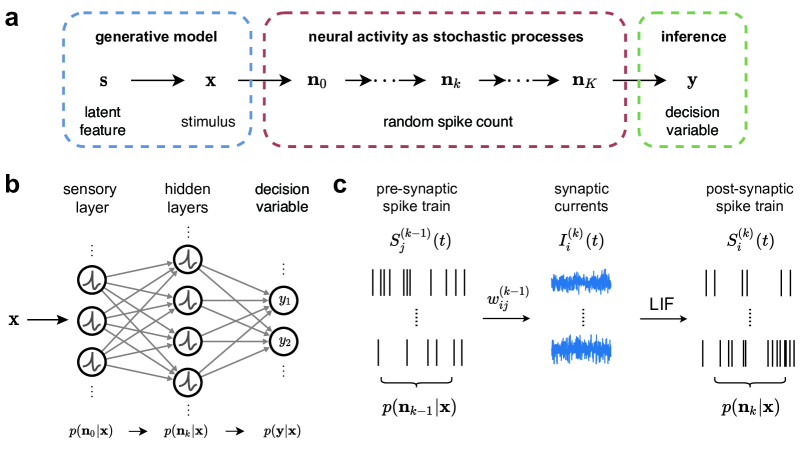
Figure 1: Spike-based stochastic neural computing (SNC). a, A graphical model for SNC which consists of a generative model describing the external environment, multiple stages of fluctuating neural activity states, and a readout for making inference. The index $k$ represents different neural populations in a feedforward network or alternatively time in a recurrent network. b, Schematics of a spiking neural network implementing the computational processes outlined in a, with each layer characterized by a joint probability distribution of neural spike count. c, Propagation of irregular neural spike trains through two feedforwardly connected neural populations. The pre-synaptic spike trains first undergo synaptic summation to generate fluctuating synaptic currents, which in turn drive post-synaptic neurons to fire. The probability distribution of spike count is transformed in a non-trivial way due to the nonlinear coupling of correlated neural variability.

We first lay the general theoretical foundation for stochastic neural computing (SNC). Consider a computational process shown in Fig. 1, which consists of three components. The first component is a generative model describing how an observable stimulus $\mathbf{x}$ (such as an image) in the environment depends on its latent features $\mathbf{s}$. The second component is a model describing the fluctuating activity states $\mathbf{n}_{k}$ of a group of neural populations, which are interpreted as random spike counts over a time window $\Delta t$. The index $k$ represents different neural populations in a feedforward network or alternatively discrete time steps in a recurrent network. The last component is a decision variable or readout $\mathbf{y}$ representing behavioral response.

To express these computation stages concretely, we write down the distribution $p(\mathbf{n}_{k}|\mathbf{x})$ of the neural population state $\mathbf{n}_{k}$ at each stage $k$ in terms of the marginalization of its conditional probability over $\mathbf{n}_{k-1}$ in the preceding stage as

$$p(\mathbf{n}_{k}|\mathbf{x})=\int p(\mathbf{n}_{k}|\mathbf{n}_{k-1},\mathbf{x})p(\mathbf{n}_{k-1}|\mathbf{x})d\mathbf{n}_{k-1}.$$ (1)

By chaining equation (1) iteratively, we recover the probability of the readout $\mathbf{y}$ conditioned on the stimulus $\mathbf{x}$

$$p(\mathbf{y}|\mathbf{x})=\int p(\mathbf{y}|\mathbf{n}_{K},\mathbf{x})\prod_{k=1}^{K}p(\mathbf{n}_{k}|\mathbf{n}_{k-1},\mathbf{x})p(\mathbf{n}_{0}|\mathbf{x})d\mathbf{n}_{0}\cdots d\mathbf{n}_{K}.$$ (2)

Equipped with this conceptual framework, we can now define SNC as a series of neural operations [equation (1)] that generates a desired conditional distribution $p(\mathbf{y}|\mathbf{x})$ of the readout $\mathbf{y}$ given a stimulus $\mathbf{x}$. Under this view, the fundamental computing unit of SNC is the probability distribution of the activity state of a neural population $p(\mathbf{n})$, and the basic operation of SNC is the transformation of these distributions across populations of neurons.

A spiking neural network implementing this computational process is illustrated in Fig. 1b where each neuron in the network is modeled as a leaky integrate-and-fire (LIF) neuron [see equation (5)-(6) in Methods]. One step of SNC carried out across two populations of spiking neurons is shown in more detail in Fig. 1c. As irregular spike trains from the pre-synaptic population converge at post-synaptic neurons, they give rise to fluctuating synaptic currents and subsequently irregular spike emissions in the post-synaptic neurons ²⁴. Importantly, since these fluctuating synaptic currents are generated from a common pool of pre-synaptic neurons, they inevitably become correlated even if the input spikes are not. These correlated neural fluctuations are further transformed in a nonlinear fashion as they propagate across downstream neural populations.

To perform any useful computation, the spiking neural network needs to learn the set of parameter values $\theta$ that matches the readout distribution $p(\mathbf{y}|\mathbf{x};\theta)$ with a desired target distribution $p^{*}(\mathbf{y}|\mathbf{x})$. The probabilistic interpretation of the readout $\mathbf{y}$ allows us to design learning objectives (loss functions) in a principled manner ²⁵. Here we prescribe two such loss functions for regression and classification tasks under the supervised learning setting. For regression problems, a natural choice is the negative log likelihood

$$L(\theta)=-\sum_{\mathbf{x}\in\mathcal{D}}\log p(\mathbf{y}^{*}|\mathbf{x};\theta),$$ (3)

where $p(\mathbf{y}^{*}|\mathbf{x};\theta)$ is the likelihood of the network parameters $\theta$ for when $\mathbf{y}=\mathbf{y}^{*}$ with $\mathbf{y}^{*}$ representing target output. For classification problems, class prediction is obtained by taking the class label $i$ corresponding to the largest entry of $\mathbf{y}$. The probability that the model predicts class $i$ for a given input $\mathbf{x}$ can be expressed as $q_{i}(\theta)=\int p(\mathbf{y}|\mathbf{x};\theta)\mathbf{1}_{D_{i}}(\mathbf{y})d\mathbf{y}$, where the indicator function $\mathbf{1}_{D}(\mathbf{y})$ is equal to one if $\mathbf{y}\in D$ and zero otherwise, and $D_{i}$ denotes the set of all $\mathbf{y}$ whose largest entry is $y_{i}$. Denoting $t$ as the target class, the goal is then to maximize the probability of correct prediction $q_{t}$. This leads to the loss function

$$L(\theta)=-\sum_{\mathbf{x}\in\mathcal{D}}\log(q_{t})=-\sum_{\mathbf{x}\in\mathcal{D}}\int p(\mathbf{y}|\mathbf{x};\theta)\mathbf{1}_{D_{t}}(\mathbf{y})d\mathbf{y},$$ (4)

Interestingly, the same expression can be alternatively obtained from cross entropy $H(\theta)=-\sum_{i}p_{i}\log(q_{i})=-\log(q_{t})$ with $p_{i}=1$ for $i=t$ and zero otherwise. Our formulation can thus be considered as a natural generalization of cross entropy loss commonly used in deterministic artificial neural networks. The physical significance of equation (4) is that by minimizing $L(\theta)$ the spiking neural network can be trained to make correct predictions while simultaneously minimizing trial-to-trial variability.

Although the general theoretical framework presented above provides a useful conceptual guide, question remains as how the spiking neural network under such probabilistic representation can be computed and trained. Direct evaluation of equation (2) is computationally infeasible at large scale and it is unclear how learning algorithms such as backpropagation can be implemented with respect to fluctuating neural activity. To resolve this problem, we propose a moment embedding which parameterizes the probability distributions of neural spiking activity in terms of their first- and second-order statistical moments.

2.2 A moment embedding for gradient-based learning in spiking neural network

The moment embedding characterizes fluctuating neural spike count with its first- and second-order statistical moments, that is, the mean firing rate $\mu$ and the firing co-variability $C$. Through a diffusion formalism ³³, we can derive on a mathematically rigorous ground the mapping from the statistical moments of the pre-synaptic neural activity to that of the synaptic current, and from the synaptic current to the post-synaptic neural activity. This leads to a class of neural network models known as the moment neural network (MNN) which faithfully captures spike count variability up to second-order statistical moments ³¹, ³². This can be considered as a minimalistic yet rich description of stochastic neural dynamics characterizing all pairwise neural interactions. The moment embedding essentially provides a finite-dimensional parameterization of joint probability distributions of neural spiking activity through which gradient-based learning can be performed. The network parameters trained this way can then be used directly to recover the spiking neural network without fining tuning of free parameters. An overall schematic illustrating this concept is shown in Fig. 2a. Details of the moment embedding are given by equation (8-14) in Methods.

The basic building block of the MNN is a single feedforward layer as illustrated in Fig. 2b. By mapping the mean firing rate and firing covariability of the pre-synaptic population to that of the post-synaptic population, this feedforward layer essentially implements one step of stochastic neural computing in equation (1) which maps $p(\mathbf{n}_{k-1}|\mathbf{x})$ to $p(\mathbf{n}_{k}|\mathbf{x})$. Multiple layers can be stacked together to form a complete chain implementing equation (2). This feedforward layer has three key components, namely, synaptic summation, moment activation, and moment batch normalization.

For the mean firing rate, the synaptic summation works similarly as in standard rate models by calculating the synaptic current mean as a weighted sum of the pre-synaptic mean firing rate [equation (10)]. Unlike rate models, however, the same synaptic weights are also used to transform the second-order moments [equation (11)], resulting in correlated synaptic currents even if the input spikes are uncorrelated. The moment activation [equation (12-14)] provides the moment mapping through which the input current mean and covariance become nonlinearly coupled to produce the post-synaptic spike mean and covariance ³¹, ³², ²⁴. Figure 2c illustrates the components in the moment activation for the leaky integrate-and-fire spiking neuron model.

The moment batch normalization is designed to overcome the vanishing gradient problem in deep networks, which occurs when the inputs are sufficiently strong (or weak), causing the saturation (or vanishing) of the moment activation function and subsequently the failure of gradient propagation. For conventional rate-based activation functions such as sigmoid functions, this problem is effectively alleviated through batch normalization ³⁴. Here, we propose a generalized batch normalization incorporating second-order moments, referred to as the moment batch normalization [see equation (17)-(18) in Methods]. A key property of the moment batch normalization is that a common normalization factor is shared between the mean and variance of the synaptic current, so that its parameters can be re-absorbed into the synaptic weights and external input currents after training is complete, thereby preserving the structure of the original spiking neural network (see equation (21)-(22).

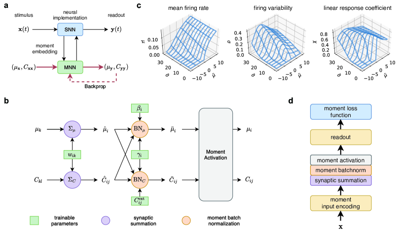
Figure 2: Gradient-based learning in spiking neural network through moment embedding. a, Overall schematics. The spiking neural network model is first mapped to a corresponding moment neural network which can be trained with backpropagation; the trained weights are used to recover the original spiking neural network. b, Computational graph of a single feedforward layer of the moment neural network, featuring synaptic summation, moment batch normalization and moment activation. c, Components of the moment activation function including mean firing rate $\mu$, firing variability $\sigma$, and the linear response coefficient $\chi$, each of which is a function of the input current mean $\bar{\mu}$ and variability $\bar{\sigma}$. In conventional analog and digital computing, such noise coupling is considered detrimental to information carried within the signal. In contrast, stochastic computing actively exploits correlated variability as a part of the computational processes. d, Illustration of a trainable moment neural network with a feedforward architecture consisting of an input layer, arbitrary number of hidden layers, a readout layer, and a moment loss function.

By stacking the building block of MNN, one can construct a deep network of arbitrary depth. To enable gradient-based learning, it is also necessary to specify an appropriate moment embedding for the input and an objective function incorporating second-order moments. For illustrative purposes, here we assume independent Poisson input encoding. We also derive moment embedding for the loss functions from equation (3)-(4) to arrive at a generalized mean-squared error loss for regression problems and a moment cross entropy loss for classification problems [see equation (19) and (20) in Methods]. Figure  2d shows an example of a complete feedforward MNN consisting of a Poisson-encoded input layer, a hidden layer, a linear readout, and a moment loss function.

2.3 Stochastic neural computing with correlated variability

Having developed the basic building blocks of MNN, we now demonstrate our learning framework for SNC with a classification task. For illustrative purposes, we consider a fully connected, feedforward MNN for implementing supervised learning on the MNIST datasest ³⁵ consisting of images of hand-written digits. A single hidden layer and a Poisson-rate input encoding scheme are used. See Methods for details of model set-up.

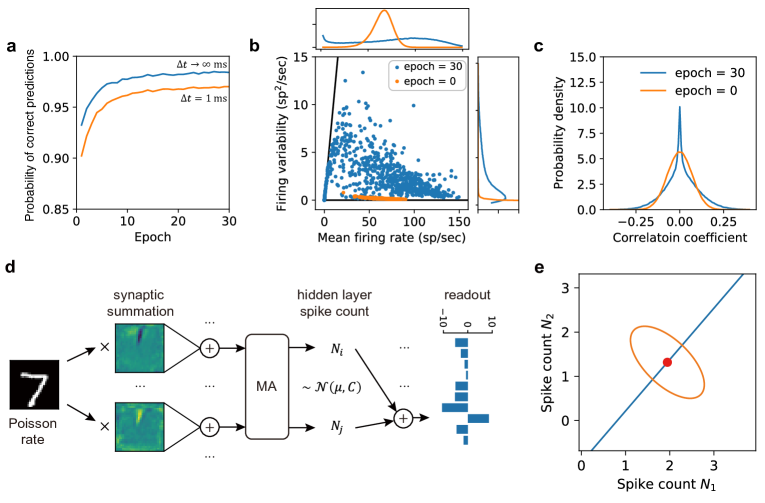
Figure 3: Moment neural network learning classification task while simultaneously minimizing uncertainty. a, The probability of correct prediction averaged over all samples of the validation set during training for unlimited and limited readout time $\Delta t$; the latter takes into account of trial-to-trial variability. For unlimited readout time ($\Delta t\to\infty$), the accuracy reaches $98.3\%$ at the end of the epochs, comparable to the performance of rate-based artificial neural networks. b, Diverse firing variability of hidden layer neurons in response to the input image shown in e, exhibiting both mean-dominant (Fano factor close to zero) and fluctuation-dominant (Fano factor close to one, solid line) activity. Insets: probability densities. c, Spike count correlation of the hidden layer neurons exhibit weak correlation whose distribution shows a slower decaying tail after training. d, Illustration of non-trivial roles played by correlated variability of a specific pair of hidden layer neurons. An input image represented by independent Poisson spike trains undergoes synaptic summation with anti-correlated weights, leading to anti-correlated neural activity. The final readout is linearly decoded from the hidden layer spike counts. e, The mean (dot) and covariance (ellipse) of the spike count of those two neurons over a readout time $\Delta t=100$ ms. In this example, the principal axis of the covariance is orthogonal to the direction of the readout weights (solid line) with respect to the target class, leading to a reduction in the readout variance and simultaneously an increase in the readout mean.

Figure 3a shows the classification accuracy, measured as the probability of correct prediction [$q_{t}$ in equation (4)] averaged across all images in the validation set, increases with training epochs. When the readout time is infinite [$\Delta t\to\infty$ in equation (4)], this simply reflects the fraction of correctly classified samples like in a rate-based artificial neural network. In contrast to rate models, however, the MNN can also express uncertainty (trial-to-trial variability) when the readout time is finite, as reflected by a lower probability of correct prediction. Note that as $\Delta t$ increases the two curves converge.

In addition, the hidden layer exhibits diverse firing variability consistent with cortical neurons ³, ³⁶, ³⁷. Fig. 3b shows the neural response to a typical sample image, with each point corresponding to a neuron. The mean firing rate and firing variability of the hidden layer neuron cover a broad range of values, from fluctuation-dominant activity (closer to Fano factor of one, solid line) to mean-dominant activity (closer to Fano factor of zero, x-axis). In contrast, a network with random initialization before training has narrowly distributed firing variability. The pairwise correlations of the hidden layer neurons are also weakly correlated, with both positive and negative values centered around the origin [Fig. 3(c)]. This result is consistent with that observed in cortical neurons ³⁷, and also satisfies the assumptions behind the linear response analysis used to derive the correlation mapping in equation (14). Interestingly, we find that the distribution of the correlation coefficients exhibits a longer tail after training.

To provide an intuitive understanding about the role played by correlated neural variability, we now focus on a specific pair of neurons in the hidden layer and trace the computational steps involved in producing $y_{t}$, the readout component corresponding to the target class. As shown in Fig. 3d, an input image encoded by independent Poisson spikes with $\mu_{0}=\sigma^{2}_{0}$ first undergoes synaptic summation to produce correlated synaptic currents, which in turn elicit neural responses $(\mu_{1},C_{1})$ in the hidden layer. For the specific pair of neurons shown, the synaptic weights have opposite patterns, resulting in negatively correlated neural responses. Figure 3e illustrates the joint distribution of spike count ($\Delta t=100$ ms) for this neuronal pair, with their mean firing rate marked by the dot and their covariance highlighted by the ellipse. Remarkably, the principal axis of the covariance, in this 2D projection, is orthogonal to the line representing the readout weights from these two neurons to the target class [solid line in Fig. 3e]. As a result, the readout effectively projects the spike count distribution in the hidden layer along its principal axis, leading to reduced uncertainty in $y_{t}$.

2.4 Re-mapping to spiking neural network with zero free parameter

Because the MNN is analytically derived from the LIF spiking neuron model, recovering the spiking neural network (SNN) from a trained MNN is straightforward. No further post-training optimization or fining tuning is required. First, an input image is encoded into independent Poisson spike trains, which then undergo synaptic summation according to equation (6). The synaptic weights and the external currents $I^{\rm ext}_{i}$ are recovered by absorbing the moment batch normalization into the summation layer of the trained MNN according to equation (22). Finally, the readout $\mathbf{y}(t)$ is calculated from the spike count $\mathbf{n}(\Delta t)$ over a time window of duration $\Delta t$ according to equation (7). It becomes evident that the readout $\mathbf{y}(\Delta t)$ follows a distribution $p(\mathbf{y}|\mathbf{x};\theta)$ with mean $\mu(\theta)$ and covariance $\tfrac{1}{\Delta t}C(\theta)$ as output by the MNN. The class corresponding to the largest entry in the readout $\mathbf{y}(\Delta t)$ is then taken as the class prediction.

As consistent with the MNN, the recovered SNN exhibits both mean-dominant and fluctuation-dominant spiking activity as shown in Fig. 3a. For a typical neuron with mean-dominant activity, the synaptic current it receives has a positive mean and weak temporal fluctuations. As a result, the sub-threshold membrane potential of the neuron consistently ramps up over time, resulting in spike emission at relatively regular intervals. In contrast, a neuron with fluctuation-dominant activity is largely driven by a synaptic current with large fluctuations even though its mean is close to zero, resulting in spike emission at highly variable intervals. Such diverse firing variability is a key feature of SNC, even if the neuronal model itself is deterministic. The spike raster plot of hidden layer neurons in the SNN in response to an input image [the same as in Fig. 3d] is shown in Fig. 4b.

To reveal the temporal dynamics of the readout, we show in Fig. 4c a 2D projection of the readout trajectories $\mathbf{y}(\Delta t)$ in response to the same image over different trials. When $\Delta t$ is small, the readouts from individual trials are scattered over a wide area, corresponding to a larger trial-to-trial variability. As more spikes are accumulated with increasing $\Delta t$, the trajectory of the readout in a single trial also fluctuates over time, and eventually converges toward the readout mean $\mu$ [marked with the dot in Fig. 4c] as predicted by the MNN. Since the magnitude of the fluctuations in the readout tends to decrease over time, this may potentially provide a way for the brain to infer confidence during a single trial and potentially an early stopping criterion for decision making.

To further quantify how task performance depends on readout time, we simulate the SNN over 100 trials for each image in the validation set of MNIST, and calculate the probability of correct prediction [$q_{t}$ in equation (4)] for different input images as the readout time $\Delta t$ increases. As can be seen from the result for four randomly picked images shown in Fig. 4d, $q_{t}$ increases with the readout time rapidly and eventually reaches one within around 5 ms, with some images require less time than others. A similar pattern is found for $q_{t}$ when plotted as a function of spike count (measured by binning individual trials based on the population spike count of hidden layer neurons) which directly reflects the energy cost.

When averaged over all images, the probability of correct prediction reveals an exponential convergence toward the theoretical limit of $0.985$ as predicted by the MNN with a short time constant of $\tau=0.95$ ms (left panel in Fig. 4e). A short burn-in time of around 1 ms is due to the membrane potential being initialized to zero. This rapid convergence results in short decision latency, with an average probability of correct response of 95% obtained in less than 5 ms. This is largely due to that the moment cross entropy explicitly takes into account of trial-to-trial variability for finite readout time, so that the neural network learns to improve the rate of convergence without requiring knowledge of precise spike timing. A similar exponential convergence for $q_{t}$ averaged over all images is found with respect to the spike count, with a decay constant of around 50 spikes. A reasonably accurate prediction of 95% can be achieved with less than 200 spikes. This exceptional energy efficiency is largely due to that a large proportion of the neural population in our model is fluctuation-dominant [Fig. 3(a)], with an average firing rate of 50 sp/s across the entire network.

To further demonstrate our method, we implement the SNN trained through moment embedding on Intel’s Loihi neuromorphic chip and provide benchmarking results in terms of accuracy, energy cost, and latency. See Supplementary Information for details.

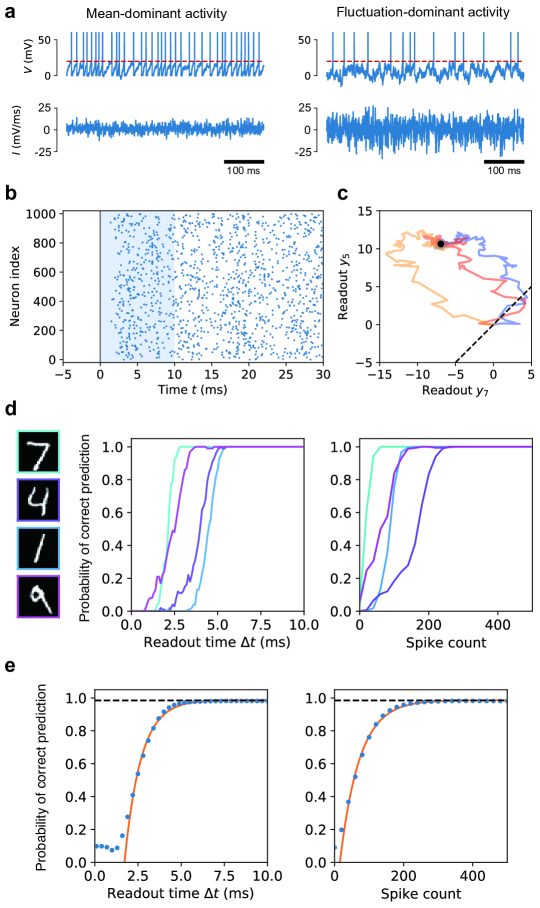
Figure 4: Temporal dynamics of stochastic neural computing in spiking neural network. a, Membrane potential (upper panel) and synaptic current (lower panel) of two typical hidden layer neurons during one trial of stimulus presentation, each exhibiting mean-dominant (left panel) and fluctuation-dominant (right panel) activity. Dashed line indicates firing threshold. b, Raster plot of typical spiking activity of hidden layer neurons during one trial of stimulus presentation. Solid line indicates stimulus onset at $t=0$ ms; shaded region indicates the readout time window $\Delta t$. The membrane potential of all neurons are initialized to zero at $\Delta t=0$ ms. c, Two dimensional projection of the readout trajectory $y$ over time for three trials using the same stimulus. The vertical axis is the readout component corresponding to the correct class. Dot indicates theoretical limit of the readout mean as $\Delta t\to\infty$; dashed line indicates the decision boundary. d, Probability of correct prediction for a number of input images (left panel) as a function of readout time and population spike count. Each curve is calculated from $100$ trials with the same stimulus. e, Probability of correct prediction averaged over all images of the validation set converges exponentially with the readout time (left panel) as well as the population spike count (panel); dashed lines indicate the theoretical limit of $0.985$ as predicted by the MNN. Solid lines represent exponential fits.

3 Discussion

The general framework of stochastic neural computing (SNC) based on moment embedding as proposed in this work has a number of advantages. First, the moment embedding approach provides an effective finite-dimensional parameterization of joint probability distributions of neural population activity up to second-order statistical moments, through which probabilistic neural operations can be efficiently computed. Second, derived from spiking neural models on a mathematically rigorous ground, the moment embedding faithfully captures the nonlinear coupling of correlated neural variability and the propagation of neural correlation across large populations of spiking neurons. Lastly, the differentiability of the moment mapping enables backpropagation for gradient-based learning, leading to a new class of deep learning model referred to as the moment neural network (MNN).

The MNN naturally generalizes standard artificial neural network (ANN) in deep learning to second-order statistical moments and provides a conceptual link between biological SNN and ANN, and between spike-time coding and rate coding. Although the example presented here only considers a feedforward architecture, the moment embedding approach can be used to systematically generalize many of the known deep learning architectures, such as convolutional and recurrent neural networks, to second-order statistical moments. The moment embedding approach also provides an alternative algorithm for training SNNs based on probabilistic codes. Unlike ANN-to-SNN conversion methods in the deep learning literature, which requires extensive post-training optimization such as threshold balancing to mitigate performance loss caused by conversion ³⁸, the parameters trained through the moment embedding can be used directly to recover the SNN without further fining tuning. See Supplemental Information for further discussion.

The proposed framework of SNC incorporates uncertainty into the learning objective and further enables direct manipulations of correlated neural variability in a task-driven way. Specifically, the moment embedding approach enables end-to-end learning of arbitrary probabilistic computation tasks, and provides significant advantage over conventional handcrafted approach to constructing neural circuit model for probabilistic neural computation which often rely on prior assumptions regarding the specific form of neural code or simplifications for facilitating theoretical analysis. Our theory of SNC also emphasizes uncertainty representation through stochastic processes of neural spike trains, through which signal and noise are processed concurrently rather than through different channels such as in a variational auto-encoder.

The approach developed in this paper also has broader implications to stochastic computing, which has been proposed as an alternative computing architecture for approximate computation with better error tolerance and energy efficiency ³⁹, ⁴⁰. However, designing stochastic computing circuits for arbitrary functions remains a major challenge. Our method indicates a solution to this problem by training SNNs for implementing spike-based SNC. Combined with advances in neuromorphic hardware ⁴¹, ⁴², ⁴³, the principle of SNC could lead to a future generation of brain-inspired computing architecture.

4 Methods

4.1 Leaky integrate-and-fire neuron model

The membrane potential dynamics of a leaky integrate-and-fire (LIF) neuron is described by

$$\dfrac{dV_{i}}{dt}=-LV_{i}(t)+I_{i}(t),$$ (5)

where the sub-threshold membrane potential $V_{i}(t)$ of a neuron $i$ is driven by the total synaptic current $I_{i}(t)$ and $L=0.05$ ${\mathrm{ms}}^{-1}$ is the leak conductance. When the membrane potential $V_{i}(t)$ exceeds a threshold $V_{\rm th}=20$ $\mathrm{mV}$ a spike is emitted, as represented with a Dirac delta function. Afterward, the membrane potential $V_{i}(t)$ is reset to the resting potential $V_{\rm res}=0$ mV, followed by a refractory period $T_{\rm ref}=5$ ms. The synaptic current takes the form

$$I_{i}(t)=\sum_{j}w_{ij}S_{j}(t)+I_{i}^{\rm ext}(t),$$ (6)

where $S_{j}(t)=\sum_{k}\delta(t-t^{k}_{j})$ represents the spike train generated by pre-synaptic neurons.

A final output $\mathbf{y}$ is readout from the spike count $\mathbf{n}(\Delta t)$ of a population of spiking neurons over a time window of duration $\Delta t$ as follows

$$y_{i}(\Delta t)=\frac{1}{\Delta t}\sum_{j}w_{ij}n_{j}(\Delta t)+\beta_{i},$$ (7)

where $w_{ij}$ and $\beta_{i}$ are the weights and biases of the readout, respectively. One property of the readout is that its variance should decrease as the readout time window $\Delta t$ increases.

4.2 Moment embedding for the leaky integrate-and-fire neuron model

The proposed moment embedding approach begins with mapping the fluctuating activity of spiking neurons to their respective first- and second-order moments

$$\mu_{i}=\lim_{\Delta t\to\infty}\dfrac{\mathbb{E}[n_{i}(\Delta t)]}{\Delta t},$$ (8)

and

$$C_{ij}=\lim_{\Delta t\to\infty}\dfrac{{\rm Cov}[n_{i}(\Delta t),n_{j}(\Delta t)]}{\Delta t},$$ (9)

where $n_{i}(\Delta t)$ is the spike count of neuron $i$ over a time window $\Delta t$. In practice, the limit of $\Delta t\to\infty$ is interpreted as a sufficiently large time window relative to the time scale of neural fluctuations. We refer the moments $\mu_{i}$ and $C_{ij}$ as the mean firing rate and the firing co-variability, respectively.

For the LIF neuron model [equation (5)], the statistical moments of the synaptic current is equal to ³¹, ³²

$$\hat{\mu}_{i}=\textstyle\sum_{k}w_{ik}\mu_{k}+\hat{\mu}_{i}^{\rm ext},$$ (10)

$$\hat{C}_{ij}=\textstyle\sum_{kl}w_{ik}C_{kl}w_{jl}+\hat{C}_{ij}^{\rm ext},$$ (11)

where $w_{ik}$ is the synaptic weight and $\hat{\mu}_{i}^{\rm ext}$ and $\hat{C}_{ij}^{\rm ext}$ are the mean and covariance of an external current, respectively. Note that from equation (11), it becomes evident that the synaptic current are correlated even if the pre-synaptic spike trains are not. Next, the first- and second-order moments of the synaptic current is mapped to that of the spiking activity of the post-synaptic neurons. For the LIF neuron model, this mapping can be obtained in closed form through a mathematical technique known as the diffusion approximation ³¹, ³² as

$$\mu_{i}=\phi_{\mu}(\bar{\mu}_{i},\bar{\sigma}_{i}),$$ (12)

$$\sigma_{i}=\phi_{\sigma}(\bar{\mu}_{i},\bar{\sigma}_{i}),$$ (13)

$$\rho_{ij}=\chi(\bar{\mu}_{i},\bar{\sigma}_{i})\chi(\bar{\mu}_{j},\bar{\sigma}_{j})\bar{\rho}_{ij},$$ (14)

where the correlation coefficient $\rho_{ij}$ is related to the covariance as $C_{ij}=\sigma_{i}\sigma_{j}\rho_{ij}$. In this paper, we refer this mapping given by equation (12)-(14) as the moment activation.

The functions $\phi_{\mu}$ and $\phi_{\sigma}$ together map the mean and variance of the input current to that of the output spikes according to ³¹, ³²

$$\phi:(\bar{\mu},\bar{\sigma}^{2})\mapsto(\mu,\sigma^{2}),~{}~{}~{}~{} \mu=\dfrac{1}{T_{\rm ref}+\tfrac{2}{L}\int_{I_{\rm lb}}^{I_{\rm ub}}g(x)dx},$$ (15)

$$\phi:(\bar{\mu},\bar{\sigma}^{2})\mapsto(\mu,\sigma^{2}),~{}~{}~{}~{} \sigma^{2}=\tfrac{8}{L^{2}}\mu^{3}\textstyle\int_{I_{\rm lb}}^{I_{\rm ub}}h(x)dx,$$ (16)

where $T_{\rm ref}$ is the refractory period with integration bounds $I_{\rm ub}(\bar{\mu},\bar{\sigma})=\tfrac{V_{\rm th}L-\bar{\mu}}{\sqrt{L}\bar{\sigma}}$ and $I_{\rm lb}(\bar{\mu},\bar{\sigma})=\tfrac{V_{\rm res}L-\bar{\mu}}{\sqrt{L}\bar{\sigma}}$. The constant parameters $L$, $V_{\rm res}$, and $V_{\rm th}$ are identical to those in the LIF neuron model in equation (5). The pair of Dawson-like functions $g(x)$ and $h(x)$ appearing in equation (15) and equation (16) are $g(x)=e^{x^{2}}\int_{-\infty}^{x}e^{-u^{2}}du$ and $h(x)=e^{x^{2}}\int_{-\infty}^{x}e^{-u^{2}}[g(u)]^{2}du$. The function $\chi$, which we refer to as the linear perturbation coefficient, is equal to $\chi(\bar{\mu},\bar{\sigma})=\tfrac{\bar{\sigma}}{\sigma}\tfrac{\partial\mu}{\partial\bar{\mu}}$ and it is derived using a linear perturbation analysis around $\bar{\rho}_{ij}=0$ ³². This approximation is justified as pairwise correlations between neurons in the brain are typically weak. An efficient numerical algorithm is used for evaluating the moment activation and its gradients ⁴⁴.

4.3 Moment batch normalization

The moment batch normalization for the input mean $\hat{\mu}_{i}$ is

$$\bar{\mu_{i}}=\dfrac{\hat{\mu}_{i}-\mathbb{E}[\hat{\mu}_{i}]}{\sqrt{\nu_{i}+\epsilon}}\gamma_{i}+\beta_{i},$$ (17)

where $\mathbb{E}[\hat{\mu}_{i}]$ is the mean computed over samples within a mini-batch and $\nu_{i}$ is a normalization factor. The bias $\beta_{i}$ and scaling factor $\gamma_{i}$ are trainable parameters, similar to that in the standard batch normalization. The key difference from the standard batch normalization for firing rate model is the normalization factor which must accommodate the effect of input fluctuations. In this study, we propose the following form of normalization factor, $\nu_{i}={\rm Var}[\hat{\mu}_{i}]+\mathbb{E}[\hat{\sigma}^{2}_{i}]$, which involves the expectation of the input variance in addition to the variance of the input mean. In fact, by invoking the law of total variance, it can be shown that this particular choice of normalization factor can be interpreted as the variance of the total synaptic current $I_{i}(t)$ [equation (6)] in the corresponding SNN, that is, ${\rm Var}[\hat{\mu}_{i}]+\mathbb{E}[\hat{\sigma}^{2}_{i}]={\rm Var}[I_{i}(t)]$, where the variance on the right-hand side is evaluated across the mini-batch as well as time. Note that the standard batch normalization used in rate-based ANN corresponds to the special case of equation (17) when the input current $I_{i}(t)$ is constant, that is, when $\hat{\sigma}^{2}_{i}=0$.

The moment batch normalization for the input covariance $\hat{C}_{ij}$ enforces the same normalization factor $\nu_{i}$ and trainable $\gamma_{i}$ as used in equation (17) but without centering. The shared normalization factor and trainable factor allow the moment batch normalization to be absorbed into the synaptic weights after training is complete, thereby preserving the link to the underlying spiking neural network. This leads to

$$\bar{C}_{ij}=\dfrac{\hat{C}_{ij}}{\sqrt{(\nu_{i}+\epsilon)(\nu_{j}+\epsilon)}}\gamma_{i}\gamma_{j}+C_{ij}^{\rm ext},$$ (18)

where $C_{ij}^{\rm ext}$ represents the covariance of an external input current. To ensure symmetry and positive semi-definiteness of the covariance matrix, we set $C^{\rm ext}=A^{T}A$ with the matrix $A$ being a trainable parameter with the same size as $C^{\rm ext}$. Alternatively, for independent external input current, we set $C^{\rm ext}_{ij}=\delta_{ij}(\sigma^{\rm ext}_{i})^{2}$, with $\sigma_{i}^{\rm ext}$ being trainable parameters. In practice, the computation of equation (18) can be quite cumbersome and one way to significantly simplify this step, with some reduced flexibility, is to consider the special case where the external input covariance $C_{ij}^{\rm ext}$ is zero. Under this scenario, we only need to apply batch normalization to the variance and pass directly the off-diagonal entries via the correlation coefficient, $\bar{\rho}_{ij}=\hat{\rho}_{ij}$. Similar to the standard batch normalization, the input mean and input variance over minibatch are replaced by the running mean and running variance during the validation phase. A schematic diagram showing the moment batch normalization is shown in Fig. 2.

A practical benefit of the moment batch normalization is that it simplifies parameter initialization before training as we can initialize of the parameters $(\beta_{i},\gamma_{i},C_{ij}^{\rm ext})$ to appropriate values so that the total post-synaptic current $(\bar{\mu}_{i},\bar{\sigma}_{i})$ is always within a desired working regime, regardless of the task or the input sample.

4.4 Moment loss functions

Assuming a Gaussian-distributed readout and substituting its probability density

$$p(\mathbf{y}|\mathbf{x};\theta)=\tfrac{1}{\sqrt{\det(2\pi C)}}\exp\left[-\tfrac{1}{2}(\mathbf{y}-\mu)^{T}C^{-1}(\mathbf{y}-\mu)\right]$$

into each of equation (3)-(4) lead to the following objective functions expressed in terms of the second-order statistical moments of the readout.

For regression problems, the principle of maximum likelihood leads to

$$L(\theta)=(\mu-\mathbf{y}^{*})^{T}C^{-1}(\mu-\mathbf{y}^{*})\Delta t+\log\det(\tfrac{2\pi}{\Delta t}C),$$ (19)

where $\mathbf{y}^{*}$ represents the readout target and $t$ represents matrix transpose. We refer this loss function as the moment mean-squared error (MMSE) loss. This loss function simultaneously minimizes the difference between the output mean $\mu$ and the target $\mathbf{y}^{*}$ (systematic error) in the first term as well as the output covariance (random error) in the second term. The readout time $\Delta t$ controls the trade-off between accuracy and precision, that is, a smaller $\Delta t$ prioritizes reducing the random error more than the systematic error and vice versa. Interestingly, equation (19) can be interpreted as a form of free energy, such that the first and the second terms correspond to the energy and the entropy of the system, respectively. The standard mean-squared error (MSE) loss is a special case of equation (19) for when $C=I$. In practice, a small positive value (representing a constant external background noise) is added to the diagonal entries of $C$ to avoid numerical instability during matrix inversion.

For classification problems, class prediction is obtained by taking the class label $i$ corresponding to the largest entry of $\mathbf{y}$. Since there is no simple analytical expression for the probability of correct predictions $q_{i}(\theta)=\int p(\mathbf{y}|\theta)\mathbf{1}_{D_{i}}(\mathbf{y})d\mathbf{y}$ in high dimensions, we use a finite-sample approximation such that $q_{i}\approx\tfrac{1}{N}\sum_{n=1}^{N}\mathbf{1}_{D_{i}}(\mathbf{y}^{n})$, with $\mathbf{y}^{n}$ being a multivariate normal random variable with mean $\mu$ and covariance $\tfrac{1}{\Delta t}C$. To generate the random samples, we perform Cholesky decomposition $C=LL^{T}$ to express $\mathbf{y}^{n}$ as $\mathbf{y}^{n}=L\mathbf{z}^{n}+\mu$, where $\mathbf{z}^{n}$ is an uncorrelated unit normal random variable. Importantly, the Cholesky decomposition $L$ is differentiable with respect to $C$, allowing for backpropagation to be implemented. Next, to solve the non-differentiability of the indicator function, we approximate it with the soft-max function $\mathbf{1}_{D_{i}}(\mathbf{y})\approx\sigma_{i}(\mathbf{y};\beta)=\exp(\beta y_{i})/\sum_{i}\exp(\beta y_{i})$, where $\beta$ is a steepness parameter such that $\sigma_{i}(\mathbf{y};\beta)\to\mathbf{1}_{D_{i}}(\mathbf{y})$ as $\beta\to\infty$. Combining all these steps we obtain the following generalized cross-entropy loss

$$H(\theta)\approx-\log\sum_{n=1}^{N}\sigma_{t}(\tfrac{1}{\sqrt{\Delta t}}L\mathbf{z}^{n}+\mu;\beta),$$ (20)

which we refer to as the moment cross-entropy (MCE) loss (here $t$ denotes target class). Note that the standard cross-entropy loss commonly used in deep learning corresponds to a special case of equation (20) when the readout time is unlimited, that is, when $\Delta t\to\infty$.

4.5 Recovering synaptic weights in spiking neural network

The synaptic weights $\tilde{w}_{ij}$ and the moments of the external currents $I^{\rm ext}_{i}(t)$ are recovered by absorbing the moment batch normalization into the summation layer of the trained MNN according to the formulae

$$\mu_{i}^{\rm ext}=\beta_{i}-\tfrac{\gamma_{i}}{\sqrt{\nu_{i}+\epsilon}}\mathbb{E}[\hat{\mu}_{i}],$$ (21)

$$\tilde{w}_{ij}=\tfrac{\gamma_{i}}{\sqrt{\nu_{i}+\epsilon}}w_{ij},$$ (22)

where $w_{ij}$ is the synaptic weight of the summation layer in the trained MNN; the quantities $\mathbb{E}[\hat{\mu}_{i}]$, $\nu_{i}={\rm Var}[\hat{\mu}_{i}]+\mathbb{E}[\hat{\sigma}^{2}_{i}]$, $\beta_{i}$ and $\gamma_{i}$ are the running mean, running variance, bias and scaling factor in the moment batch normalization [equation (17)-(18)]. The covariance of the external current $C_{ij}^{\rm ext}$ is the same as that in equation (18). The external current $I^{\rm ext}_{i}(t)$ to the spiking neural network can therefore be reconstructed as a Gaussian white noise with mean $\mu_{i}^{\rm ext}$ and covariance $C_{ij}^{\rm ext}$, and in turn be fed into the LIF neuron model in equation (6). No further post-training optimization or fining tuning is required during this reconstruction procedure.

4.6 Model setup for training

We train the moment neural network on the MNIST dataset which contains 60000 images for training and 10000 images for validation. The model consists of an input layer, a hidden layer and a readout layer. For this task, the number of neurons is 784 for the input layer, 1000 for the hidden layer, and 10 for the readout. For the input layer, a Poisson-rate encoding scheme is used such that neurons in the input layer emits independent Poisson spikes with rates proportional to the pixel intensity $\mathbf{x}$, that is, $\mu_{0}=\sigma^{2}_{0}=\alpha\mathbf{x}$, where $\alpha$ is the stimulus transduction factor set to be $\alpha=1$ spikes per ms, and the correlation coefficient $\rho_{ij}=0$ for $i\neq j$. The hidden layer involves synaptic summation [equation (10)-(11)], followed by moment batch normalization [equation (17)-(18)] and then by moment activation [equation (12)-(14)]. The readout mean $\mu$ and covariance $\tfrac{1}{\Delta t}C$ are calculated using equation (10)-(11) where the readout time is set to be $\Delta t=1$ ms. The moment cross entropy loss [equation (20)] is used to train the network. with the number of random samples set to be $n=1000$ and the steepness parameter to $\beta=1$ during training. The model is implemented in Pytorch and trained with stochastic gradient descent (AdamW). Gradients are evaluated using Pytorch’s autograd functionality, except for the moment activation in which custom gradients for equation (12)-(14) are used ⁴⁴.

Code Availability

The code for simulating and training the moment neural network (MNN) model is available without restrictions on Github (https://github.com/BrainsoupFactory/moment-neural-network).

Author Contributions

Conceptualization: Y.Q. and J.F.; Methodology: Y.Q., W.L. and J.F.; Investigation: Y.Q., Z.Z. and Y.W.; Software: Y.Q., Z.Z. and Y.W.; Resources and deployment supporting: Z.W. and L.C.; Visualization: Y.Q. and Z.Z.; Writing — original draft: Y.Q. and Z.Z.; Writing — review & editing: Y.Q., Z.Z., Z.W., L.C., W.L., and J.F.; Supervision: J.F.

Competing interests

The authors declare no competing interests.

Materials & Correspondence

Correspondence and requests for materials should be addressed to J.F.

S1 Comparison to existing approaches to training spiking neural networks

As in the main text, the moment embedding developed in this study leads to a novel approach to training spiking neural networks (SNN) under the principle of stochastic neural computing (SNC). Here, we briefly review existing approaches to training SNNs and compare them to ours.

Existing approaches to training SNN can largely fall into two categories: ANN-to-SNN conversion and direct SNN training methods ²⁹. In the ANN-to-SNN conversion method, a standard artificial neural network (ANN) is pre-trained using traditional backpropagation algorithms, and then converted to an SNN model by mapping the ANN parameters onto SNN. These rate-coded network conversion often results in accuracy loss and relatively high inference latency. Many works have focused on transferring weights from ANN with continuous-valued activation to SNN and setting the firing threshold of neurons layer by layer to achieve near-lossless performance but poor latency ⁴⁵, ³⁸, ⁴⁶; other approaches have also been proposed to improve the accuracy while trying to reduce the inference time steps and keep the event-driven sparsity for better energy efficiency ⁴⁷.

Direct approaches to training SNN, on the other hand, use backpropagation-through-time to optimize the parameters of an SNN directly ⁴⁸, ⁴⁹, ²⁹. This requires formulating the SNN as an equivalent recurrent neural network with binary spike inputs. This enables emergent spike-timing codes which convey information with the relative timing between spikes for efficient sparse coding. The main challenge of direct training is due to the discontinuous, non-differentiable nature of spike generation. Diverse methods have been proposed to solve the problem by defining surrogate gradient or spike time coding to enable backpropagation; some examples include spike layer error reassignment (SLAYER) ⁵⁰, spatiotemporal backpropagation (STDB) ⁵¹, and local online learning via eligibility propagation (e-prop) ³⁰. In general, direct training approaches tend to achieve fewer spikes, lower latency and energy consumption, but need to overcome difficulties on convergence and performance degradation as network size increases ²⁹.

In contrast to existing methods, the method proposed in this study is based on the principle of SNC which implements a form of probabilistic code. In contrast to conversion-based methods which require extensive post-training optimization to compensate performance loss caused by conversion, our approach is rooted in the rigorous treatment of stochastic dynamics of spiking neurons and therefore does not require fine tuning of additional free parameters. Compared to direct training method, our approach is much more efficient and scalable as it only requires backpropagation through the statistical moments of neural activity rather than through the temporally varying membrane potential.

In the following, we demonstrate the application of our method on neuromorphic hardware. Specifically, we implement a SNN trained with our approach to perform image classification task on Intel’s neuromorphic computing research chip Loihi ⁴¹, ⁴².

S2 Spiking neural network implementation on Loihi

As a research chip, Loihi is designed to support a broad range of SNNs with sufficient scale, performance, and features to deliver competitive results compared to state-of-the-art contemporary computing architectures. Loihi harnesses insights from biological neural systems to build electronic devices and to realize biological computing principles efficiently. Specifically, Loihi is a digital, event-driven asynchronous circuit chip using discrete-time computational model. Each Loihi chip contains 128 neuromorphic cores and 3 low-power embedded x86 CPU cores. Every neuromorphic core has up to 1K leaky integrate-and-fire (LIF) neurons, implementing a total of 128K neurons and 128M synaptic connections per chip for spike-based neural computing. Embedded CPU cores are mainly used for management as well as bridging between conventional and neuromorphic hardware. Single Loihi chip could show orders of magnitude improvements in terms of low power consumption and fast processing speed on certain tasks compared with conventional hardware.

Loihi implements a discretized version of the LIF neuron model as follows

$$V_{i}(t) =(1-\tfrac{1}{\tau_{v}})V_{i}(t-1)+I_{i}(t)+\beta,$$ (S1)

$$I_{i}(t) =(1-\tfrac{1}{\tau_{u}})I_{i}(t-1)+\sum_{j}w_{ij}s_{j}(t),$$ (S2)

where $V_{i}(t)$ and $I_{i}(t)$ represent the membrane potential and synaptic current received by the $i$th neuron at a discrete time step $t$, respectively, and $s_{j}(t)$ represents binary spike trains of pre-synaptic neurons. The quantities $\tau_{v}$, $\tau_{u}$, and $\beta$ represent the membrane time constant, synaptic time constant, and bias current, respectively.

The following parameter setting is used to match the discrete LIF model [equation (S2)] implemented by Loihi to the continuous LIF model [equation (5)] in the main text. First, the synaptic current time constant $\tau_{u}$ is set to be infinite so that the synaptic current becomes a weighted sum of input spikes. Second, we use exact solution of the subthreshold membrane potential rather than the Euler scheme for numerical integration to accommodate larger simulation time step $\delta t$, which is often desirable for saving energy on hardware. As a result, the membrane time constant is set to be $\frac{1}{\tau_{v}}=1-e^{-L\delta t}$ and the bias current is set to be $\beta_{i}=\tfrac{1}{L}(1-e^{-L\delta t})I_{i}^{\rm ext}$, where $I_{i}^{\rm ext}$ is the external input current in the continuous model. By default, we set $L=0.05$ ${\mathrm{ms}}^{-1}$ and $\delta t=1$ ms.

Since Loihi only supports 9-bit signed integer representation of synaptic weights taking values in the range $[-256,254]$, appropriate rescaling is needed to map the synaptic weights from physical units to this 9-bit representation. Specifically, a factor of $k=\frac{254}{\max(|\hat{w}^{\rm MNN}|)}$ is used to scale the synaptic weight, the membrane potential and the bias currents, which are rounded down to integer values afterward.

One nuance regarding the hardware implementation is how to emulate the linear readout [equation (7)] used in the continuous model. This is achieved with an output layer consisting of perfect integrator neurons ($L=0$) with infinite firing threshold. Under this setting, the linear readout $y$ is equivalent to the membrane potential in the output layer divided by the readout time $T$, which can be recorded by the hardware. The model prediction is based on the output neuron with the highest membrane potential.

S3 Details of benchmarking results

To demonstrate, we implement the spiking neural network (SNN) trained using our method to perform MNIST image classification task on Intel’s neuromorphic chip Loihi. Unless otherwise specified, the network structure is the same as in the main text. We first perform off-chip training of the moment neural network and then transfer the trained synaptic weights to SNN using equation (21)-(22) in Methods. For this purpose, we use the moment loss function [equation (20)] with $\Delta t$ set to be infinite as this setting gives the best result on Loihi. Then, the model parameters are rescaled and quantized to satisfy Loihi’s hardware constraints as discussed above. For hardware implementation, the stimulus transduction factor is set to be $\alpha=0.1$ sp/ms for encoding training sample (see Method in main text). This further limits the overall number of spikes and thus energy consumption.

Performance of hardware implementation of an SNN is typically characterized by a number of key metrics including accuracy, energy consumption, and latency (also known as delay). Accuracy measures the fraction of correctly predicted samples in the dataset averaged across trials. Energy consumption measures in joule the dynamic energy consumed by the neuromorphic cores per inference, whereas delay measures the elapsed wall time per inference. Both energy consumption and delay are measured by the on-board probe of Loihi Nahuku-32 board using NxSDK version 2.0.

We first check the consistency in prediction accuracy between the SNN implemented on Loihi and that implemented on CPU. As shown in Fig. S1a, the prediction accuracy of the SNN model deployed on Loihi increases with time and approaches to the theoretical limit predicted by the MNN (dashed line in Fig. S1a). Compared to the single-precision floating-point implementation on CPU, the Loihi implementation has a small amount of accuracy loss caused by the 9-bit weight quantization. Nonetheless, the result is impressive considering no fining tuning of free parameters are applied after training.

On neuromorphic hardware, it is often desirable to use a coarser time step $\delta t$ to reduce energy consumption and delay. As shown in Fig. S1b, both energy consumption and delay (in wall time) are roughly inversely proportional to $\delta t$ for fixed simulation duration ($T=100$ ms). However, the accuracy on neuromorphic hardware deteriorates with coarser time discretization (Fig. S1c). This is due to that the model parameters are trained under the assumption of continuous LIF model rather than its discrete version. In practice, we find that this accuracy deterioration is negligible for $\delta t$ much smaller than the membrane potential time constant $1/L=20$ ms. To strike a balance between accuracy and energy consumption, we set $\delta t=1$ ms for the remaining results. Despite the present limitation, the general approach of moment embedding can be extended in the future to overcome this problem by deriving directly the moment mapping for the discrete SNN model rather than the continuous one.

As indicated by our general theory of SNC, there is a direct relationship between the uncertainty expressed by MNN and the required decision time, which in turn impacts the energy consumption. This suggests a potential way to optimize the trade-off between accuracy, energy cost, and delay on neuromorphic hardware. In the following, we investigate how the energy cost and delay depend on the hyperparameters of MNN during training. All models are trained over 30 epochs and the energy profiles are calculated through the first 1000 samples of the test dataset.

Specifically, we analyze how the hidden layer size and the readout time window $\Delta t$ used in the loss function [equation (20)] affect the model performance on Loihi. Moment neural networks with one hidden layer of different sizes (for $n=$ 64, 128, 256, 512, 1024) are trained under different values of $\Delta t$ in the moment loss function (for $\Delta t=$ 1, 2, 5, 10 ms). These models’ performances as measured by accuracy, energy consumption, and delay are summarized in Fig. S1.

We first look at the performance metrics after the accuracy fully converges at $t=100$ ms. As shown in Fig. S1d, a larger hidden layer size in general leads to better accuracy, but the improvement becomes less significant at larger sizes. The final accuracy is also improved by a larger readout time $\Delta t$ in the moment cross entropy loss used during the training. This is consistent with our theoretical prediction as a smaller $\Delta t$ prioritize accuracy at shorter time scales at the detriment of the accuracy at long time scales. As shown in Fig. S1e, the energy consumption (measured as the dynamic energy per sample) increases linearly with the hidden layer size and is largely unaffected by $\Delta t$ used during training. This is expected as energy cost is approximately proportional to the number of spikes and to the network size provided that the overall firing rate is fixed. As shown in Fig. S1f, the latency per sample does not show a clear trend across different network size or $\Delta t$ (with an exception at very small network size of $n=64$). This is because the primary factor determining latency (wall time) is the model simulation time which is fixed at $t=100$ ms.

As can be seen from results above, the performance as measured by accuracy, energy consumption, and delay have complex dependency on model hyperparameters, suggesting a potential way to optimize the trade-off between them. Specifically, we would like to know how we can achieve the best energy-delay product for any given level of accuracy. For this purpose, we identify the simulation time when each model reaches 80% of accuracy and then record the corresponding energy consumption and delay. The results are best visualized using an energy-delay diagram as shown in Fig. S1h. Each curve represents the energy-delay characteristic profile for achieving a fixed level of accuracy as the hidden layer size varies. We find that a larger hidden layer size generally leads to less latency but at the cost of higher energy, whereas larger $\Delta t$ generally leads to better efficiency in both energy consumption and latency. Using the energy-delay diagram we can conveniently choose the appropriate network size to achieve an optimal trade-off between energy consumption and latency.

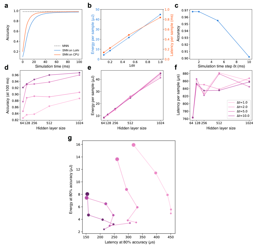
Figure S1: Performance of SNN deployed on neuromorphic chip. a, Classification accuracy increases with simulation time steps and converges to the theoretical limit predicted by the MNN. Compared to single-precision floating-point simulation on CPU, the simulation on Loihi has a small amount of accuracy loss caused by weight quantization. b, The classification accuracy over time of each model. c, The classification accuracy (at 100 ms of simulation time) for varying hidden layer size and $\Delta t$ used in loss for training. d, The average energy cost per sample (at 100 ms of simulation time) for varying hidden layer sizes and $\Delta t$. e, The average latency (at 100 ms of simulation time) for varying hidden layer size and $\Delta t$. f, Energy-latency diagram (at 80% accuracy) revealing a trade-off between energy cost and latency. The dot size corresponds to hidden layer size and the color corresponds to the value of $\Delta t$ used during training.

References

- 1 Tomko, G. J. & Crapper, D. R. Neuronal variability: non-stationary responses to identical visual stimuli. Brain Res. 79, 405–418 (1974).
- 2 Tolhurst, D., Movshon, J. & Dean, A. The statistical reliability of signals in single neurons in cat and monkey visual cortex. Vision Res. 23, 775–785 (1983).
- 3 Softky, W. R. & Koch, C. The highly irregular firing of cortical cells is inconsistent with temporal integration of random EPSPs. J. Neurosci. 13, 334–350 (1993).
- 4 Arieli, A., Sterkin, A., Grinvald, A. & Aertsen, A. Dynamics of ongoing activity: explanation of the large variability in evoked cortical responses. Science 273, 1868–1871 (1996).
- 5 Deco, G., Rolls, E. T. & Romo, R. Stochastic dynamics as a principle of brain function. Prog. Neurobiol. 88, 1–16 (2009).
- 6 Fiser, J., Berkes, P., Orbán, G. & Lengyel, M. Statistically optimal perception and learning: from behavior to neural representations. Trends Cogn. Sci. 14, 119–130 (2010).
- 7 Maass, W. Noise as a resource for computation and learning in networks of spiking neurons. Proceedings of the IEEE 102, 860–880 (2014).
- 8 Knill, D. C. & Richards, W. (eds.) Perception as Bayesian Inference (Cambridge University Press, 1996).
- 9 Yuille, A. & Kersten, D. Vision as Bayesian inference: analysis by synthesis? Trends Cogn. Sci. 10, 301–308 (2006).
- 10 Griffiths, T. L., Steyvers, M. & Tenenbaum, J. B. Topics in semantic representation. Psychol. Rev. 114, 211 (2007).
- 11 Vul, E., Goodman, N., Griffiths, T. L. & Tenenbaum, J. B. One and done? Optimal decisions from very few samples. Cognitive Sci. 38, 599–637 (2014).
- 12 Wolpert, D. M. Probabilistic models in human sensorimotor control. Hum. Movement Sci. 26, 511–524 (2007).
- 13 Ma, W. J. & Jazayeri, M. Neural coding of uncertainty and probability. Annu. Rev. Neurosci. 37, 205–220 (2014).
- 14 Hénaff, O. J., Boundy-Singer, Z. M., Meding, K., Ziemba, C. M. & Goris, R. L. Representation of visual uncertainty through neural gain variability. Nat. Commun. 11, 1–12 (2020).
- 15 Ma, W. J., Beck, J. M., Latham, P. E. & Pouget, A. Bayesian inference with probabilistic population codes. Nat. Neurosci. 9, 1432–1438 (2006).
- 16 Hoyer, P. & Hyvärinen, A. Interpreting neural response variability as Monte Carlo sampling of the posterior. In Becker, S., Thrun, S. & Obermayer, K. (eds.) Adv. Neur. In., vol. 15 (MIT Press, 2002).
- 17 Panzeri, S., Schultz, S. R., Treves, A. & Rolls, E. T. Correlations and the encoding of information in the nervous system. Proc. R. Soc. Lond. B Biol. Sci. 266, 1001–1012 (1999).
- 18 Kohn, A., Coen-Cagli, R., Kanitscheider, I. & Pouget, A. Correlations and neuronal population information. Annu. Rev. Neurosci. 39, 237–256 (2016).
- 19 Ding, M. & Glanzman, D. The Dynamic Brain: an Exploration of Neuronal Variability and its Functional Significance (Oxford University Press, USA, 2011).
- 20 Averbeck, B. B., Latham, P. E. & Pouget, A. Neural correlations, population coding and computation. Nat. Rev. Neurosci. 7, 358–366 (2006).
- 21 Buesing, L., Bill, J., Nessler, B. & Maass, W. Neural dynamics as sampling: a model for stochastic computation in recurrent networks of spiking neurons. PLOS Comput. Biol. 7, 1–22 (2011).
- 22 Orbán, G., Berkes, P., Fiser, J. & Lengyel, M. Neural variability and sampling-based probabilistic representations in the visual cortex. Neuron 92, 530–543 (2016).
- 23 Qi, Y. & Gong, P. Fractional neural sampling as a theory of spatiotemporal probabilistic computations in neural circuits. Nat. Commun. 13, 4572 (2022).
- 24 Rocha, J. d. l., Doiron, B., Shea-Brown, E., Josić, K. & Reyes, A. Correlation between neural spike trains increases with firing rate. Nature 448, 802–806 (2007).
- 25 Jang, H., Simeone, O., Gardner, B. & Grning, A. An introduction to probabilistic spiking neural networks. IEEE Signal Proc. Mag. 36, 64–77 (2019).
- 26 Schneidman, E., Berry, M. J., Segev, R. & Bialek, W. Weak pairwise correlations imply strongly correlated network states in a neural population. Nature 440, 1007–1012 (2006).
- 27 Panzeri, S., Moroni, M., Safaai, H. & Harvey, C. D. The structures and functions of correlations in neural population codes. Nat. Rev. Neurosci. 1–17 (2022).
- 28 Ma, H., Qi, Y., Gong, P., Lu, W. & Feng, J. Dynamics of bump attractors in neural circuits with emergent spatial correlations (2022). arXiv:2212.01663.
- 29 Pfeiffer, M. & Pfeil, T. Deep learning with spiking neurons: opportunities and challenges. Front. Neurosci. 12, 774 (2018).
- 30 Bellec, G. et al. A solution to the learning dilemma for recurrent networks of spiking neurons. Nat. Commun. 11, 3625 (2020).
- 31 Feng, J., Deng, Y. & Rossoni, E. Dynamics of moment neuronal networks. Phys. Rev. E 73, 041906 (2006).
- 32 Lu, W., Rossoni, E. & Feng, J. On a Gaussian neuronal field model. NeuroImage 52, 913–933 (2010).
- 33 Fourcaud, N. & Brunel, N. Dynamics of the firing probability of noisy integrate-and-fire neurons. Neural Comput. 14, 2057–2110 (2002).
- 34 Ioffe, S. & Szegedy, C. Batch normalization: accelerating deep network training by reducing internal covariate shift (2015). arXiv:1502.03167.
- 35 Deng, L. The MNIST database of handwritten digit images for machine learning research. IEEE Signal Proc. Mag. 29, 141–142 (2012).
- 36 Ponce-Alvarez, A., Thiele, A., Albright, T. D., Stoner, G. R. & Deco, G. Stimulus-dependent variability and noise correlations in cortical mt neurons. Proc. Natl. Acad. Sci. 110, 13162–13167 (2013).
- 37 Rosenbaum, R., Smith, M. A., Kohn, A., Rubin, J. E. & Doiron, B. The spatial structure of correlated neuronal variability. Nat. Neurosci. 20, 107–114 (2017).
- 38 Diehl, P. U. et al. Fast-classifying, high-accuracy spiking deep networks through weight and threshold balancing. In 2015 International Joint Conference on Neural Networks (IJCNN), 1–8 (2015).
- 39 Gaines, B. R. Stochastic computing systems. In Advances in Information Systems Science, vol. 2, 37–172 (Springer, 1969).
- 40 Alaghi, A., Qian, W. & Hayes, J. P. The promise and challenge of stochastic computing. IEEE Transactions on Computer-aided Design of Integrated Circuits and Systems 37, 1515–1531 (2018).
- 41 Davies, M. et al. Advancing neuromorphic computing with Loihi: a survey of results and outlook. Proceedings of the IEEE 109, 911–934 (2021).
- 42 Davies, M. et al. Loihi: a neuromorphic manycore processor with on-chip learning. IEEE Micro 38, 82–99 (2018).
- 43 Dutta, S. et al. Neural sampling machine with stochastic synapse allows brain-like learning and inference. Nat. Commun. 13, 2571 (2022).
- 44 Qi, Y. An efficient numerical algorithm for the moment neural activation (2022). arXiv:2212.01480.
- 45 Rueckauer, B., Lungu, I.-A., Hu, Y., Pfeiffer, M. & Liu, S.-C. Conversion of continuous-valued deep networks to efficient event-driven networks for image classification. Front. Neurosci. 11 (2017).
- 46 Yan, Z., Zhou, J. & Wong, W.-F. Near lossless transfer learning for spiking neural networks. Proceedings of the AAAI Conference on Artificial Intelligence 35, 10577–10584 (2021).
- 47 Rathi, N., Srinivasan, G., Panda, P. & Roy, K. Enabling deep spiking neural networks with hybrid conversion and spike timing dependent backpropagation (2020). arXiv:2005.01807.
- 48 Yan, Y. et al. Backpropagation with sparsity regularization for spiking neural network learning. Front. Neurosci. 16, 760298 (2022).
- 49 Lee, J. H., Delbruck, T. & Pfeiffer, M. Training deep spiking neural networks using backpropagation. Front. Neurosci. 10, 508 (2016).
- 50 Shrestha, S. B. & Orchard, G. SLAYER: Spike layer error reassignment in time. Adv. Neur. In. 31 (2018).
- 51 Wu, Y., Deng, L., Li, G., Zhu, J. & Shi, L. Spatio-temporal backpropagation for training high-performance spiking neural networks. Front. Neurosci. 12 (2018).
Supplementary Information
Toward spike-based stochastic neural computing
Yang Qi1,2,3, Zhichao Zhu1, Yiming Wei1, Lu Cao4, Zhigang Wang4, Wenlian Lu1,2, Jianfeng Feng1,2,*
1 Institute of Science and Technology for Brain-Inspired
Intelligence, Fudan University, Shanghai 200433, China
2 Key Laboratory of Computational Neuroscience and Brain-Inspired
Intelligence (Fudan University), Ministry of Education, China
3 MOE Frontiers Center for Brain Science, Fudan University, Shanghai 200433, China
4 Intel Labs China, Beijing, 100190, China