Decoupled Kullback-Leibler Divergence Loss

Abstract

In this paper, we delve deeper into the Kullback–Leibler (KL) Divergence loss and observe that it is equivalent to the Doupled Kullback-Leibler (DKL) Divergence loss that consists of 1) a weighted Mean Square Error ($w$MSE) loss and 2) a Cross-Entropy loss incorporating soft labels. From our analysis of the DKL loss, we have identified two areas for improvement. Firstly, we address the limitation of DKL in scenarios like knowledge distillation by breaking its asymmetry property in training optimization. This modification ensures that the $w$MSE component is always effective during training, providing extra constructive cues. Secondly, we introduce global information into DKL for intra-class consistency regularization. With these two enhancements, we derive the Improved Kullback–Leibler (IKL) Divergence loss and evaluate its effectiveness by conducting experiments on CIFAR-10/100 and ImageNet datasets, focusing on adversarial training and knowledge distillation tasks. The proposed approach achieves new state-of-the-art performance on both tasks, demonstrating the substantial practical merits. Code and models will be available soon at https://github.com/jiequancui/DKL.

1 Introduction

Loss functions are a critical component of training deep models. Cross-Entropy loss is particularly important in image classification tasks He et al. (2016); Simonyan and Zisserman (2015); Tan et al. (2019); Dosovitskiy et al. (2020); Liu et al. (2021), while Mean Square Error (MSE) loss is commonly used in regression tasks Ren et al. (2015); He et al. (2017, 2022). Contrastive loss Chen et al. (2020a); He et al. (2020); Chen et al. (2020b); Grill et al. (2020); Caron et al. (2020); Cui et al. (2021a, 2023) has emerged as a popular objective for representation learning. The selection of an appropriate loss function can exert a substantial influence on a model’s performance. Therefore, the development of effective loss functions Cao et al. (2019); Lin et al. (2017); Zhao et al. (2022); Wang et al. (2020); Johnson et al. (2016); Berman et al. (2018); Wen et al. (2016); Tan et al. (2020) remains a critical research topic in the fields of computer vision and machine learning.

Kullback-Leibler (KL) Divergence quantifies the degree of dissimilarity between a probability distribution and a reference distribution. As one of the most frequently used loss functions, it finds application in various scenarios, such as adversarial training Zhang et al. (2019); Wu et al. (2020); Cui et al. (2021b); Jia et al. (2022), knowledge distillation Hinton et al. (2015); Chen et al. (2021); Zhao et al. (2022), incremental learning Chaudhry et al. (2018); Lee et al. (2017), and robustness on out-of-distribution data Hendrycks et al. (2019). Although many of these studies incorporate KL Divergence loss as part of their algorithms, they may not thoroughly investigate the underlying mechanisms of the loss function. To address this issue, our paper aims to elucidate the working mechanism of KL Divergence during training optimization.

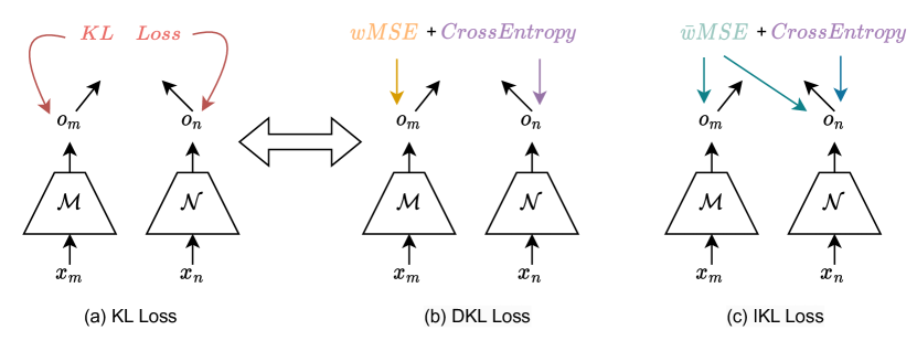
Figure 1: The proposed DKL and IKL losses. $\mathcal{M}$ and $\mathcal{N}$ can be the same one or two separate models determined by application scenarios. Similarly, $x_{m}$, $x_{n}$ $\in$ $\mathcal{X}$ can also be the same one or two different images. $o_{m}$, $o_{n}$ are logits output with which the probability vector can be obtained when applying the Softmax activation. Black arrows represent the forward process while colored arrows indicate the gradient backpropagation flows driven by the corresponding loss functions in the same color. “$wMSE$” is a weighted MSE loss. “$\bar{w}MSE$” is incorporated with global information.

Our study focuses on the Kullback–Leibler (KL) Divergence loss from the perspective of gradient optimization. We provide theoretical proof that it is equivalent to the Decoupled Kullback–Leibler (DKL) Divergence loss, which comprises a weighted Mean Square Error ($w$MSE) loss and a Cross-Entropy loss with soft labels. We have identified potential issues with the DKL loss. Specifically, its gradient optimization is asymmetric with respect to inputs, which can lead to the weighted MSE ($w$MSE) component being ignored in certain scenarios, such as knowledge distillation. Fortunately, it is convenient to address this issue with the formulation of DKL by breaking the asymmetry property. Moreover, global information is used to regularize the training process as a holistic categorical distribution prior. Combining DKL with these two points, we derive the Improved Kullback–Leibler (IKL) Divergence loss. Fig. 1 presents a clear visual comparison of the KL, DKL, and IKL loss functions.

To demonstrate the effectiveness of our proposed IKL loss, we evaluate it in adversarial training and knowledge distillation tasks. Our experimental results on CIFAR-10/100 and ImageNet show that the IKL loss achieves new state-of-the-art performance on both tasks. In summary, the main contributions of our work are:

• Our study provides insights into the Kullback–Leibler (KL) Divergence loss by analyzing its gradient optimization properties. In doing so, we reveal that it is mathematically equivalent to a combination of a weighted Mean Square Error ($w$MSE) loss and a Cross-Entropy loss with soft labels.

• After analyzing the Decoupled Kullback-Leibler (DKL) Divergence loss, we propose two modifications for enhancement: addressing its asymmetry property and incorporating global information. The derived Improved Kullback-Leibler (IKL) Divergence loss demonstrates improved performance.

• By utilizing the IKL loss for adversarial training and knowledge distillation, we obtain state-of-the-art results for both tasks on CIFAR-10/100 and ImageNet.

2 Related Work

Adversarial Robustness.

Since the identification of adversarial examples by Szegedy et al. Szegedy et al. (2013), the security of deep neural networks (DNNs) has gained significant attention, and ensuring the reliability of DNNs has become a prominent topic in the deep learning community. Numerous algorithms have been developed to defend against adversarial attacks. However, as highlighted by Athalye et al. Athalye et al. (2018), methods relying on obfuscated gradients can create a deceptive sense of security and remain vulnerable to strong attacks such as auto-attack Croce and Hein (2020). Adversarial training Madry et al. (2017), being the most effective method, stands out due to its consistently high performance.

Adversarial training incorporates adversarial examples into the training process. Madary et al. Madry et al. (2017) propose the adoption of the universal first-order adversary, specifically the PGD attack, in adversarial training. Zhang et al. Zhang et al. (2019) enhance model robustness by utilizing the Kullback-Leibler (KL) Divergence loss based on their theoretical analysis. Wu et al. Wu et al. (2020) introduce adversarial weight perturbation to explicitly regulate the flatness of the weight loss landscape. Cui et al. Cui et al. (2021b) leverage guidance from naturally-trained models to regularize the decision boundary in adversarial training. Additionally, various other techniques Jia et al. (2022) focusing on optimization or training aspects have also been developed.

In recent years, several works have explored the use of data augmentation techniques to improve adversarial training. Gowal et al. Gowal et al. (2021) have shown that synthesized images using generative models can enhance adversarial training and improve robustness against adversarial attacks. Wang et al. Wang et al. (2023) have demonstrated that stronger robustness can be achieved by utilizing better generative models such as the popular diffusion model Karras et al. (2022), resulting in new state-of-the-art adversarial robustness. Additionally, Addepalli et al. Addepalli et al. (2022) have made it feasible to incorporate general augmentation techniques for image classification, such as Autoaugment Cubuk et al. (2019) and CutMix Yun et al. (2019a), into adversarial training.

We have explored the mechanism of KL loss for adversarial robustness in this paper. The effectiveness of the proposed IKL loss is tested in both settings with and without synthesized data.

Knowledge distillation.

The concept of Knowledge Distillation (KD) was first introduced by Hinton et al. Hinton et al. (2015). It involves extracting "dark knowledge" from accurate teacher models to guide the learning process of student models, which often have lower capacity than their teachers. This is achieved by utilizing the Kullback-Leibler Divergence (KL) loss to regularize the output probabilities of student models, aligning them with those of their teacher models when given the same inputs. This simple yet effective technique significantly improves the generalization ability of smaller models and finds extensive applications in various domains. Since the initial success of KD Hinton et al. (2015), several advanced methods, including logits-based Cho and Hariharan (2019); Furlanello et al. (2018); Mirzadeh et al. (2020); Yang et al. (2019); Zhang et al. (2018); Zhao et al. (2022) and features-based approaches Romero et al. (2015); Tian et al. (2020); Heo et al. (2019a); Zagoruyko and Komodakis (2017); Chen et al. (2021); Heo et al. (2019b, c); Kim et al. (2018); Park et al. (2019a); Peng et al. (2019); Yim et al. (2017), have been introduced.

Logits-based methods extract only the logits output from teacher models. These methods are more general than features-based methods as there is no requirement to know the teacher model architecture, and only the logits output is needed for inputs. Several advanced methods have been proposed, including mutual learning methods like DML Zhang et al. (2018), which train students and teachers simultaneously. Another approach, DKD Zhao et al. (2022), decomposes KD into target class knowledge distillation and non-target class knowledge distillation.

Features-based methods explore to take advantage of intermediate layer features compared with logits-based methods. This kind of method usually requires knowing the architecture of teacher models. With such extra priors and features information, features-based methods are expected to achieve higher performance, which can be along with more computation or storage costs. Works Heo et al. (2019a, c); Romero et al. (2015) directly transfer the representation of teacher models to student models. ReviewKD Chen et al. (2021) distills knowledge from the integrated features of multiple layers in the teacher model.

This paper decouples the KL loss into a new formulation, i.e., DKL, and addresses the limitation of KL loss for application scenarios like knowledge distillation. With the improved version of DKL, i.e., IKL loss, our models even surpass all previous features-based methods.

3 Method

In this section, we detail the preliminary and our motivation in Sec. 3.1, and then discuss our Improved Kullback-Leibler (IKL) Divergence loss in Sec. 3.2.

3.1 Preliminary and Motivation

Revisiting Kullback-Leibler (KL) Divergence Loss.

Kullback-Leibler (KL) Divergence measures the differences between two probability distributions. For distributions $P$ and $Q$ of a continuous random variable, It is defined to be the integral:

$$D_{KL}(P||Q)=\int_{-\infty}^{+\infty}p(x)*\log\frac{p(x)}{q(x)}dx,\\$$ (1)

where $p$ and $q$ denote the probability densities of $P$ and $Q$.

KL loss is one of the most commonly used objectives in deep learning. In this paper, we study the mechanism of KL loss and test our Improved Kullback-Leibler (IKL) Divergence loss with adversarial training and knowledge distillation tasks. For adversarial training, to enhance model robustness, KL loss regularizes the output probabilities of adversarial examples to be the same as that of their corresponding clean images. Knowledge distillation algorithms adopt KL loss to let a student model mimic behaviors of one teacher model. With the transferred knowledge from the teacher, the student is expected to improve performance.

Preliminaries.

We consider image classification models that output predicted probability vectors with the Softmax activation. Assume $o_{i}\in\mathcal{R}^{C}$ is the logits output of one deep model with an image $x_{i}\in\mathcal{X}$ as input, where $C$ is the number of classes in the task. $s_{i}\in\mathcal{R}^{C}$ is the predicted probability vector and $s_{i}=\textit{Softmax}(o_{i})$. $o_{i}^{j}$ and $s_{i}^{j}$ are values for the $j$-th class in $o_{i}$ and $s_{i}$ respectively.

KL loss is applied to make $s_{m}$ and $s_{n}$ similar in many scenarios, leading to the following objective,

$$\mathcal{L}_{KL}(x_{m},x_{n})=\sum_{j=1}^{C}s_{m}^{j}*\log\frac{s_{m}^{j}}{s_{n}^{j}}.\\$$ (2)

For instance, in adversarial training, $x_{m}$ is a natural image, and $x_{n}$ is the corresponding adversarial example of $x_{m}$. $x_{m}$ and $x_{n}$ indicate the same image and are fed into the teacher and student models separately in knowledge distillation. It is worth noting that $s_{m}$ is untraceable because the teacher model is well-trained in advance and fixed in the distillation process.

Motivation.

Previous works Hinton et al. (2015); Zhao et al. (2022); Zhang et al. (2019); Cui et al. (2021b) incorporate the KL loss into their algorithms without exploring its inherent working mechanism. The objective of this paper is to uncover the driving force behind training optimization through an examination of the KL loss function. With the back-propagation rule, the derivative gradients are as follows,

$$\frac{\partial\mathcal{L}_{KL}}{\partial o_{m}^{j}} = \sum_{k=1}^{C}((\Delta m_{j,k}-\Delta n_{j,k})*(s_{m}^{k}*s_{m}^{j})),$$ (3)

$$\frac{\partial\mathcal{L}_{KL}}{\partial o_{n}^{j}} = s_{m}^{j}*(s_{n}^{j}-1)+s_{n}^{j}*(1-s_{m}^{j}),$$ (4)

where $\Delta m_{j,k}=o_{m}^{j}-o_{m}^{k}$, and $\Delta n_{j,k}=o_{n}^{j}-o_{n}^{k}$.

Taking advantage of the gradient information, we introduce a novel formulation - the Decoupled Kullback-Leibler (DKL) Divergence loss - which is presented in Remark 1. The DKL loss is expected to be equivalent to the KL loss and prove to be a more analytically tractable alternative for further exploration and study.

Remark 1

From the perspective of gradient optimization, the Kullback-Leibler (KL) Divergence loss is equivalent to the following Decoupled Kullback-Leibler (DKL) Divergence loss when $\alpha=1$ and $\beta=1$.

$$\mathcal{L}_{DKL}(x_{m},x_{n})\!=\!\underbrace{\frac{\alpha}{4}\sum_{j=1}^{C}\sum_{k=1}^{C}((\Delta m_{j,k}\!-\!\mathcal{S}(\Delta n_{j,k}))^{2}*\mathcal{S}(w_{m}^{j,k}))}_{\textbf{weighted MSE ($w$MSE)}}\underbrace{-\beta\sum_{j=1}^{C}\mathcal{S}(s_{m}^{j})*\log s_{n}^{j}}_{\textbf{Cross-Entropy }},$$ (5)

where $\mathcal{S}(\cdot)$ means stop gradients operation. $w_{m}^{j,k}$ = $s_{m}^{j}$ * $s_{m}^{k}$.
Proof   See Appendix.

As demonstrated by Remark 1 and Eqs. (3) (4), we can conclude the following key properties of KL and DKL.

• DKL loss is equivalent to KL loss in terms of gradient optimization. Thus, KL loss can be decoupled into a weighted Mean Square Error ($w$MSE) loss and a Cross-Entropy loss incorporating soft labels.

• Optimization is asymmetric for $o_{m}$ and $o_{n}$. The $w$MSE and Cross-Entropy losses in (5) are complementary and collaboratively work together. The asymmetry property can cause the $w$MSE to be neglected or overlooked when $o_{m}$ is untraceable, like in the knowledge distillation scenario discussed in Sec. 3.2.

• The “$w_{m}^{j,k}$” in Eq. (5) is conditioned on the prediction of $x_{m}$. Nevertheless, sample-wise predictions may be subject to significant variance, which may result in unstable training and challenging optimization problems.

3.2 Improved Kullback-Leibler (IKL) Divergence Loss

Based on the analysis in Sec. 3.1, we propose an Improved Kullback-Leibler (IKL) Divergence loss,

$$\mathcal{L}_{IKL}(x_{m},x_{n})\!=\!\underbrace{\frac{\alpha}{4}\sum_{j=1}^{C}\sum_{k=1}^{C}((\Delta m_{j,k}\!-\!\Delta n_{j,k})^{2}*\mathcal{S}(\bar{w}_{y}^{j,k}))}_{\textbf{ global weighted MSE ($\bar{w}$MSE)}}\underbrace{-\beta\sum_{j=1}^{C}\mathcal{S}(s_{m}^{j})*\log s_{n}^{j}}_{\textbf{Cross-Entropy }},$$ (6)

where $y$ is the ground-truth label for $x_{m}$. $\bar{w}_{y}\in\mathcal{R}^{C\times C}$ is the weights for class $y$.

Compared with DKL in Eq. (5), we make the following improvements: 1) breaking the asymmetry property; 2) introducing global information. The respective details are presented as follows.

Breaking the asymmetry property.

As shown in Eq. (5), the weighted MSE encourages $o_{n}$ to be similar to $o_{m}$ with the second-order information, i.e., logit differences between any two classes. The cross-entropy loss guarantees that $s_{n}$ can have the same predicted scores with $s_{m}$. Two loss terms collaboratively work together to make $o_{n}$ and $o_{m}$ similar absolutely and relatively. Discarding any one of them can lead to performance degradation.

However, because of the asymmetry property of KL/DKL, the unexpected case may occur when $s_{m}$ is detached from the gradient back-propagation, which is formulated as:

$$\mathcal{L}_{DKL}(x_{m},x_{n})\!=\!\underbrace{\frac{\alpha}{4}\sum_{j=1}^{C}\sum_{k=1}^{C}((\mathcal{S}(\Delta m_{j,k})\!-\!\mathcal{S}(\Delta n_{j,k}))^{2}*\mathcal{S}(w_{m}^{j,k}))}_{\textbf{weighted MSE ($w$MSE)}}\underbrace{-\beta\sum_{j=1}^{C}\mathcal{S}(s_{m}^{j})*\log s_{n}^{j}}_{\textbf{Cross-Entropy }},$$ (7)

where $\mathcal{S}(\cdot)$ means stop gradients operation. $w_{m}^{j,k}$ = $s_{m}^{j}$ * $s_{m}^{k}$.

As indicated by Eq. (7), the weighted MSE loss will take no effect on training optimization since all components of $w$MSE are detached from gradient propagation, which can potentially hurt the model performance. Knowledge distillation matches this case because the teacher model is fixed during distillation training.

We address this issue by breaking the asymmetry property of KL/DKL, i.e., enabling the gradients of $\mathcal{S}(\Delta n_{j,k})$. The updated formulation becomes,

$$\mathcal{L}_{DKL}(x_{m},x_{n})\!=\!\underbrace{\frac{\alpha}{4}\sum_{j=1}^{C}\sum_{k=1}^{C}((\mathcal{S}(\Delta m_{j,k})\!-\!\Delta n_{j,k})^{2}*\mathcal{S}(w_{m}^{j,k}))}_{\textbf{weighted MSE ($w$MSE)}}\underbrace{-\beta\sum_{j=1}^{C}\mathcal{S}(s_{m}^{j})*\log s_{n}^{j}}_{\textbf{Cross-Entropy }},$$ (8)

where $\mathcal{S}(\cdot)$ means stop gradients operation. $w_{m}^{j,k}$ = $s_{m}^{j}$ * $s_{m}^{k}$.

Introducing global information.

The weights for the weighted MSE of DKL in Eq. (5) is sample-wise and depends on the prediction $s_{m}$,

$$w_{m}^{j,k}=s_{m}^{j}*s_{m}^{k}.$$ (9)

However, sample-wise weights can be biased due to the individual prediction variance. We thus adopt class-wise weights for IKL loss shown in Eq. (6),

$$\bar{w}_{y}^{j,k}=\bar{s}_{y}^{j}*\bar{s}_{y}^{k}.$$ (10)

where $y$ is ground-truth label of $x_{m}$, $\bar{s}_{y}=\frac{1}{|\mathcal{X}_{y}|}\sum_{x_{i}\in\mathcal{X}_{y}}s_{i}$.

The global information injected by $\bar{w}_{y}^{j,k}$ can act as a regularization to enhance intra-class consistency and mitigate biases that may arise from sample noise.

To this end, we derive the IKL loss in Eq. (6) by incorporating these two designs.

Table 1: Ablation study on “GI” and “BA” with DKL loss. “GI” is “Global Information”, and “BA” indicates “Breaking Asymmetry”.

Index	GI	BA	Clean	AA	Descriptions
(a)	Na	Na	62.87	30.29	baseline with KL loss.
(b)	✗	✗	62.54	30.20	DKL, equivalent to KL loss
(c)	✗	✔	62.69	30.42	(b) with BA
(d)	✗	✔	66.67	29.10	(c) with $w_{m}^{j,k}=0.01$
(e)	✔	✔	66.51	31.45	(c) with GI, i.e., IKL

A case study.

We empirically examine each component of IKL on CIFAR-100 with the adversarial training task. Ablation experimental results and their setting descriptions are listed in Table 1. In the implementation, we use improved TRADES Zhang et al. (2019) as our baseline that combines with AWP Wu et al. (2020) and uses an increasing epsilon schedule Addepalli et al. (2022). The comparison between (a) and (b) shows that DKL can achieve comparable performance, confirming the equivalence to KL. The comparisons among (b), (d), and (e) validate the effectiveness of the “GI” mechanism. We also confirm the importance of “BA” with the knowledge distillation task in Sec. 4.2.

4 Experiments

To verify the effectiveness of the proposed IKL loss, we conduct experiments on CIFAR-10, CIFAR100, and ImageNet for adversarial training (Sec. 4.1) and knowledge distillation (Sec. 4.2).

4.1 Adversarial Robustness

Experimental settings. We use an improved version of TRADES Zhang et al. (2019) as our baseline, which incorporates AWP Wu et al. (2020) and adopts an increasing epsilon schedule Addepalli et al. (2022). SGD optimizer with a momentum of 0.9 is used. We use the cosine learning rate strategy with an initial learning rate of 0.2 and train models 200 epochs. The batch size is 128, the weight decay is 5e-4 and the perturbation size $\epsilon$ is set to 8 / 255. Following previous work Zhang et al. (2019); Cui et al. (2021b), standard data augmentation including random crops with 4 pixels of padding and random horizontal flip is performed for data preprocessing.

Under the setting of training with generated data, we strictly follow the training configurations in Wang et al. (2023) for fair comparisons. Our implementations are based on their open-sourced code. We only replace the KL loss with our IKL loss.

Datasets and evaluation. CIFAR-10 and CIFAR-100 are the two most popular benchmarks in the adversarial community. The CIFAR-10 dataset consists of 60,000 32$\times$32 color images in 10 classes, with 6,000 images per class. There are 50,000 training images and 10,000 test images. The more challenging CIFAR-100 has 100 classes containing 600 images each. There are 500 training images and 100 testing images per class.

Following previous work Wu et al. (2020); Cui et al. (2021b), we report the clean accuracy on natural images and adversarial robustness under auto-attack Croce and Hein (2020) with epsilon 8/255.

Comparison methods. To compare with previous methods, We categorize them into two groups according to the different types of data preprocessing:

• Methods Wu et al. (2020); Cui et al. (2021b); Liu et al. (2019) with basic augmentation, i.e., random crops and random horizontal flip.

• Methods Wang et al. (2023); Pang et al. (2022); Gowal et al. (2021) with augmentation with generative models or AutoAug Cubuk et al. (2019), CutMix Yun et al. (2019b).

Comparisons with state-of-the-art on CIFAR-100. On CIFAR-100, with the basic augmentations setting, we compare with AWP, LBGAT, LAS-AT, and ACAT. The experimental results are summarized in Table 2. Our WRN-34-10 models trained with IKL loss do a better trade-off between natural accuracy and adversarial robustness. With $\alpha=20$ and $\beta=3$, the model achieves 66.51% top-1 accuracy on natural images while 31.45% robustness under auto-attack.

We follow Wang et al. (2023) to take advantage of synthesized images generated by the popular diffusion models Karras et al. (2022). With 1M generated images, our model achieves 68.99% top-1 natural accuracy and 35.89% robustness, surpassing Wang et al. (2023) by 0.93% and 0.24% respectively. With 50M generated images, we create new state-of-the-art with WideResNet-28-10, achieving 73.85% top-1 natural accuracy and 39.18% adversarial robustness under auto-attack.

Table 2: Test accuracy (%) of clean images and Robustness (%) under AutoAttack on CIFAR-100. We highlight our results in bold whenever the value represents an improvement relative to the strongest baseline under the same training settings, and we underline them whenever the value achieves a new SOTA result under the threat model.

Dataset	Method	Architecture	Augmentation Type	Clean	AA
CIFAR-100 ($\ell_{\infty}$, $\epsilon=8/255$)	AWP Wu et al. (2020)	WRN-34-10	Basic	60.38	28.86
	LBGAT Cui et al. (2021b)	WRN-34-10	Basic	60.64	29.33
	LAS-AT Jia et al. (2022)	WRN-34-10	Basic	64.89	30.77
	ACAT Addepalli et al. (2022)	WRN-34-10	Basic	65.75	30.23
	IKL-AT	WRN-34-10	Basic	66.51	31.45
		WRN-34-10	Basic	64.08	31.67
	Sehwag et al. (2021)	WRN-34-10	1M Generated Data	65.90	31.20
	Pang et al. (2022)	WRN-28-10	1M Generated Data	62.08	31.40
	Rebuffi et al. (2021)	WRN-28-10	1M Generated Data	62.41	32.06
	Wang et al. (2023)	WRN-28-10	1M Generated Data	68.06	35.65
		WRN-28-10	50M Generated Data	72.58	38.83
	IKL-AT	WRN-28-10	1M Generated Data	68.99	35.89
		WRN-28-10	50M Generated Data	73.85	39.18

Table 3: Top-1 accuracy (%) on the ImageNet validation and training speed (sec / iteration) comparisons. $\Delta$ represents the performance improvement over the classical KD. Training speed is calculated on 4 Nvidia GeForce 3090 GPUs with a batch of 512 224x224 images. We underline the values that achieve new SOTA results. All results are the average over three trials.

Distillation Manner	Teacher	Extra Parameters	ResNet34		ResNet50
			73.31		76.16
	Student		ResNet18		MobileNet
			69.75		68.87
Features	AT Zagoruyko and Komodakis (2017)	✗	70.69		69.56
	OFD Heo et al. (2019a)	✔	70.81		71.25
	CRD Tian et al. (2020)	✔	71.17		71.37
	ReviewKD Chen et al. (2021)	✔	71.61	0.319 s/iter	72.56	0.526 s/iter
Logits	DKD Zhao et al. (2022)	✗	71.70		72.05
	KD Hinton et al. (2015)	✗	71.03		70.50
	IKL-KD	✗	71.91	0.197 s/iter	72.84	0.252 s/iter
	$\Delta$		+0.88		+2.34

Comparison with state-of-the-art on CIFAR-10. Experimental results on CIFAR-10 are listed in Table 4, with the basic augmentation setting, our model achieves 84.70% top-1 accuracy on natural images and 57.13% robustness, outperforming previous state-of-the-art by 0.96% on robustness. With extra generated data, we improve the state-of-the-art by 0.44%, achieving 67.75% robustness.

Table 4: Test accuracy (%) of clean images and robustness (%) under AutoAttack on CIFAR-10. We highlight our results in bold whenever the value represents an improvement relative to the strongest baseline under the same training settings, and we underline them whenever the value achieves a new SOTA result under the threat model.

Dataset	Method	Architecture	Augmentation Type	Clean	AA
CIFAR-10 ($\ell_{\infty}$, $\epsilon=8/255$)	Rice et al. (2020)	WRN-34-20	Basic	85.34	53.42
	LBGAT Cui et al. (2021b)	WRN-34-20	Basic	88.70	53.57
	AWP Wu et al. (2020)	WRN-34-10	Basic	85.36	56.17
	LAS-AT Jia et al. (2022)	WRN-34-10	Basic	87.74	55.52
	ACAT Addepalli et al. (2022)	WRN-34-10	Basic	82.41	55.36
	IKL-AT	WRN-34-10	Basic	85.31	57.13
	Sehwag et al. (2021)	WRN-34-10	10M Generated Data	87.00	60.60
	Rebuffi et al. (2021)	WRN-28-10	1M Generated Data	87.33	60.73
	Gowal et al. (2021)	WRN-28-10	100M Generated Data	87.50	63.38
	Wang et al. (2023)	WRN-28-10	1M Generated Data	91.12	63.35
		WRN-28-10	50M Generated Data	92.27	67.17
		WRN-28-10	20M Generated Data	92.44	67.31
	IKL-AT	WRN-28-10	1M Generated Data	90.75	63.54
		WRN-28-10	20M Generated Data	92.16	67.75

Table 5: Top-1 accuracy (%) on the CIFAR-100 validation. Teachers and students are in the same architectures. And $\Delta$ represents the performance improvement over the classical KD. We underline the values that achieve new SOTA results. All results are the average over 3 trials.

Distillation Manner	Teacher	ResNet56	ResNet110	ResNet32$\times$4	WRN-40-2	WRN-40-2	VGG13
		72.34	74.31	79.42	75.61	75.61	74.64
	Student	ResNet20	ResNet32	ResNet8$\times$4	WRN-16-2	WRN-40-1	VGG8
		69.06	71.14	72.50	73.26	71.98	70.36
Features	FitNet Romero et al. (2015)	69.21	71.06	73.50	73.58	72.24	71.02
	RKD Park et al. (2019b)	69.61	71.82	71.90	73.35	72.22	71.48
	CRD Tian et al. (2020)	71.16	73.48	75.51	75.48	74.14	73.94
	OFD Heo et al. (2019a)	70.98	73.23	74.95	75.24	74.33	73.95
	ReviewKD Chen et al. (2021)	71.89	73.89	75.63	76.12	75.09	74.84
Logits	DKD Zhao et al. (2022)	71.97	74.11	76.32	76.24	74.81	74.68
	KD Hinton et al. (2015)	70.66	73.08	73.33	74.92	73.54	72.98
	IKL-KD	71.44	74.26	76.59	76.45	74.98	74.98
	$\Delta$	+0.78	+1.16	+3.26	+1.53	+1.44	+2.00

4.2 Knowledge Distillation

Datasets and evaluation. Following previous work Chen et al. (2021); Tian et al. (2020), we conduct experiments on CIFAR-100 Krizhevsky et al. (2009) and ImageNet Russakovsky et al. (2015) to show the advantages of IKL on knowledge distillation. ImageNet Russakovsky et al. (2015) is the most challenging dataset for classification, which consists of 1.2 million images for training and 50K images for validation over 1,000 classes.

For evaluation, we report top-1 accuracy on CIFAR-100 and ImageNet validation. The training speed of different methods is also discussed.

Experimental settings. We follow the experimental settings in Zhao et al. (2022) by Zhao et al. Our implementation for knowledge distillation is based on their open-sourced code.

Specifically, on CIFAR-100, we train all models for 240 epochs with a learning rate that decayed by 0.1 at the 150th, 180th, and 210th epoch. We initialize the learning rate to 0.01 for MobileNet and ShuffleNet, and 0.05 for other models. The batch size is 64 for all models. We train all models three times and report the mean accuracy.

On ImageNet, we use the standard training that trains the model for 100 epochs and decays the learning rate for every 30 epochs. We initialize the learning rate to 0.2 and set the batch size to 512.

For both CIFAR-100 and ImageNet, we consider the distillation among the architectures having the same unit structures, like ResNet56 and ResNet20, VGGNet13 and VGGNet8. On the other hand, we also explore the distillation among architectures made up of different unit structures, like WideResNet and ShuffleNet, VggNet and MobileNet-V2.

Comparison methods. According to the information extracted from the teacher model in distillation training, knowledge distillation methods can be divided into two categories:

• Features-based methods Romero et al. (2015); Tian et al. (2020); Chen et al. (2021); Heo et al. (2019a). This kind of method makes use of features from different layers of the teacher model, which can need extra parameters and high training computational costs.

• Logits-based methods Hinton et al. (2015); Zhao et al. (2022). This kind of method only makes use of the logits output of the teacher model, which does not require knowing the architectures of the teacher model and thus is more general in practice.

Comparison with state-of-the-art on CIFAR-100. Experimental results on CIFAR-100 are summarized in Table 5 and Table 7 (in Appendix). Table 5 lists the comparisons with previous methods under the setting that the architectures of the teacher and student have the same unit structures. Models trained by IKL-KD can achieve comparable or better performance in all considered settings. Specifically, we achieve the best performance in 4 out of 6 training settings. Table 7 in Appendix shows the comparisons with previous methods under the setting that the architectures of the teacher and student have different unit structures.

Comparison with state-of-the-art on ImageNet. We empirically show the comparisons with other methods on ImageNet in Table 3. With a ResNet34 teacher, our ResNet18 achieves 71.91% top-1 accuracy. With a ResNet50 teacher, our MobileNet achieves 72.64% top-1 accuracy. Models trained by IKL-KD surpass all previous methods while saving 38% and 52% computation costs for ResNet34–ResNet18 and ResNet50–MobileNet distillation training respectively when compared with ReviewKD Chen et al. (2021).

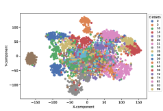
(a) IKL-AT

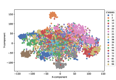
(b) TRADES

Figure 2: Visualizations by T-SNE with randomly selected 20 classes in CIFAR-100.

Table 6: Ablation study of hyper-parameters $\alpha$ and $\beta$ in IKL.

$\alpha$	Clean	AA	APGD-CE	APGD-T
$\alpha=12$	67.24	30.64	34.46	30.64
$\alpha=16$	66.60	30.72	34.43	30.72
$\alpha=20$	66.51	31.45	35.46	31.45
$\alpha=24$	63.59	31.44	35.65	31.45

(a) Effects of $\alpha$ on adversarial robustness.

$\beta$	Clean	AA	APGD-CE	APGD-T
$\beta=1$	66.68	30.69	34.22	30.66
$\beta=2$	66.56	30.80	34.70	30.80
$\beta=3$	66.51	31.45	35.46	31.45
$\beta=4$	65.45	31.08	35.44	31.08

(b) Effects of $\beta$ on adversarial robustness.

4.3 Ablation Studies

Hyper-parameters of $\alpha$ and $\beta$. With IKL, the two components can be manipulated independently. We empirically study the effects of hyper-parameters of $\alpha$ and $\beta$ on CIFAR-100 for adversarial robustness. Robustness under APGD-CE, APGD-T, and AA Croce and Hein (2020) are reported in Table 6. Especially, only samples that can not be attacked by APGD-CE will be tested under APGD-T attack. Reasonable $\alpha$ and $\beta$ should be chosen for the best trade-off between natural accuracy and adversarial robustness.

Visualization with T-SNE. We randomly sample 20 classes in CIFAR-100. The numbers in the pictures are class indexes. For each sampled class, we collect the feature representation of natural images and adversarial examples with the validation set. The visualization by T-SNE is shown in Fig. 2. Compared with TRADES that trained with KL loss, Features by IKL-AT models are more compact and separable.

5 Conclusion and Limitation

In this paper, we have investigated the mechanism of Kullback-Leibler (KL) Divergence loss in terms of gradient optimization. Based on our analysis, we decouple the KL loss into a weighted Mean Square Error ($w$MSE) loss and a Cross-Entropy loss with soft labels. The new formulation is named Decoupled Kullback-Leibler (DKL) Divergence loss. To address the spotted issues of DKL, we make two improvements that break asymmetry property in optimization and incorporate global information, deriving the Improved Kullback-Leibler (IKL) Divergence loss. Experimental results on CIFAR-10/100 and ImageNet show that we create new state-of-the-art on adversarial training and knowledge distillation tasks, indicating the effectiveness of our IKL loss. KL loss has various applications. we consider it as future work to showcase the potential of IKL in other scenarios.

Appendix A Proof to Remark 1

To demonstrate that DKL in Eq. (5) is equivalent to KL in Eq. (1) for training optimization, we prove that DKL and KL have the same gradients given the same inputs.

For KL loss, we have the following derivatives according to the chain rule:

$$\frac{\partial s_{m}^{i}}{\partial o_{m}^{i}} = s_{m}^{i}*\sum_{j!=i}^{C}s_{m}^{j},$$

$$\frac{\partial s_{m}^{j}}{\partial o_{m}^{i}} = -s_{m}^{i}*s_{m}^{j},$$

$$\frac{\partial\mathcal{L}_{KL}}{\partial s_{m}^{i}} = \log s_{m}^{i}-\log s_{n}^{i}+1,$$

$$\frac{\partial\mathcal{L}_{KL}}{\partial o_{n}^{i}} = s_{m}^{i}*(s_{n}^{i}-1)+s_{n}^{i}*(1-s_{m}^{i})$$

$$\frac{\partial\mathcal{L}_{KL}}{\partial o_{m}^{i}} = \frac{\mathcal{L}_{KL}}{\partial s_{m}^{i}}*\frac{\partial s_{m}^{i}}{\partial o_{m}^{i}}+\sum_{j!=i}^{C}\frac{\mathcal{L}_{KL}}{\partial s_{m}^{j}}*\frac{\partial s_{m}^{j}}{\partial o_{m}^{i}}$$ (11)

$$= (\log s_{m}^{i}-\log s_{n}^{i}+1)*s_{m}^{i}*\sum_{j!=i}^{C}s_{m}^{j}+\sum_{j!=i}^{C}(\log s_{m}^{j}-\log s_{n}^{j}+1)*(s_{m}^{j}*s_{m}^{i})$$

$$= \sum_{i!=j}^{C}((\log s_{m}^{i}-\log s_{m}^{j})-(\log s_{n}^{i}-\log s_{n}^{j}))*(s_{m}^{j}*s_{m}^{i})$$

$$= \sum_{i!=j}^{C}((o_{m}^{i}-o_{m}^{j})-(o_{n}^{i}-o_{n}^{j}))*(s_{m}^{j}*s_{m}^{i})$$

$$= \sum_{i!=j}^{C}(\Delta m_{i,j}-\Delta n_{i,j})*w_{m}^{i,j}$$

$$= \sum_{j}^{C}(\Delta m_{i,j}-\Delta n_{i,j})*w_{m}^{i,j}$$

For DKL los, we have the following derivatives according to the chain rule:

$$\frac{\partial\mathcal{L}_{DKL}}{\partial o_{n}^{i}} = \beta*s_{m}^{i}*(s_{n}^{i}-1)+s_{n}^{i}*(1-s_{m}^{i})$$

$$\frac{\partial\mathcal{L}_{DKL}}{\partial o_{m}^{i}} = \frac{\alpha}{4}*2*(\sum_{j}^{C}(\Delta m_{j,i}-\Delta n_{j,i})*(-w_{m}^{j,i})+\sum_{k}^{C}(\Delta m_{i,k}-\Delta n_{i,k})*w_{m}^{i,k})$$ (12)

$$= \alpha*\sum_{j}^{C}(\Delta m_{i,j}-\Delta n_{i,j})*w_{m}^{i,j}$$

Combining with Eqs. (11), (12), we claim that DKL loss and KL loss enjoy the same derivatives give the same inputs. Thus, DKL loss is equivalent to KL loss in training optimization.

Appendix B More Comparisons on CIFAR-100 for Knowledge Distillation

We experiment on CIFAR-100 with the case that the teacher and student models have different unit network architectures. The results are listed in Table 7.

Table 7: Top-1 accuracy (%) on the CIFAR-100 validation. Teachers and students are in different architectures. And $\Delta$ represents the performance improvement over the classical KD. We underline the values that achieve new SOTA results. All results are the average over 3 trials.

Distillation Manner	Teacher	ResNet32$\times$4	WRN-40-2	VGG13	ResNet50	ResNet32$\times$4
		79.42	75.61	74.64	79.34	79.42
	Student	ShuffleNet-V1	ShuffleNet-V1	MobileNet-V2	MobileNet-V2	ShuffleNet-V2
		70.50	70.50	64.60	64.60	71.82
Features	FitNetRomero et al. (2015)	73.59	73.73	64.14	63.16	73.54
	RKDPark et al. (2019b)	72.28	72.21	64.52	64.43	73.21
	CRDTian et al. (2020)	75.11	76.05	69.73	69.11	75.65
	OFDHeo et al. (2019a)	75.98	75.85	69.48	69.04	76.82
	ReviewKDChen et al. (2021)	77.45	77.14	70.37	69.89	77.78
Logits	DKD Zhao et al. (2022)	76.45	76.70	69.71	70.35	77.07
	KDHinton et al. (2015)	74.07	74.83	67.37	67.35	74.45
	IKL-KD	76.64 $\pm$ 0.02	77.19 $\pm$ 0.01	70.40 $\pm$ 0.03	70.62 $\pm$ 0.08	77.16 $\pm$ 0.04
	$\Delta$	+2.57	+2.63	+3.03	+3.27	+2.71

Appendix C More Ablations for Adversarial Robustness

As described in Sec. 3.2, corporating global information, the class-wise weights is proposed to promote intra-class consistency and mitigate the biases from sample noise,

$$\bar{w}_{y}^{j,k}=\bar{s}_{y}^{j}*\bar{s}_{y}^{k}.$$ (13)

where $y$ is ground-truth label of $x_{m}$, $\bar{s}_{y}=\frac{1}{|\mathcal{X}_{y}|}\sum_{x_{i}\in\mathcal{X}_{y}}s_{i}$.

We further examine the effect of temperature $\tau$ and extend the class-wise weights as,

$$\bar{w}_{y}^{j,k}=\bar{s}_{y}^{j}*\bar{s}_{y}^{k}.$$ (14)

where $y$ is ground-truth label of $x_{m}$, $\bar{s}_{y}=\frac{1}{|\mathcal{X}_{y}|}\sum_{x_{i}\in\mathcal{X}_{y}}s_{i}$, and $s_{i}=\textit{Softmax}(o_{i}/\tau)$.

Table 8: Ablation study of temperature $\tau=4$ for global information.

Hyper-parameter $\tau=4$ with $\alpha$	Clean	AA
$\alpha=12$	67.24	30.64
$\alpha=16$	66.60	30.72
$\alpha=20$	66.51	31.45
$\alpha=24$	63.59	31.44

(a) Effects of $\alpha$ with $\beta=3$.

Hyper-parameter $\tau=4$ with $\beta$	Clean	AA
$\beta=1$	66.68	30.69
$\beta=2$	66.56	30.80
$\beta=3$	66.51	31.45
$\beta=4$	65.45	31.08

(b) Effects of $\beta$ with $\alpha=20$.

Table 9: Ablation study of temperature $\tau=2$ for global information.

Hyper-parameter $\tau=2$ with $\alpha$	Clean	AA
$\alpha=15$	65.12	31.17
$\alpha=18$	64.63	31.34
$\alpha=20$	64.31	31.59
$\alpha=24$	63.59	31.44

(a) Effects of $\alpha$ with $\beta=3$.

Hyper-parameter $\tau=2$ with $\beta$	Clean	AA
$\beta=2$	64.30	31.46
$\beta=3$	64.31	31.59
$\beta=4$	64.08	31.67
$\beta=5$	63.58	31.62

(b) Effects of $\beta$ with $\alpha=20$.

Appendix D Code and Pre-trained Models

On adversarial training with CIFAR-100 and CIFAR-10, we achieve the new state-of-the-art in both settings with/without data augmentations. Our pre-trained models are available to be evaluated.

• CIFAR-100 (clean 66.51 AA 31.45): https://drive.google.com/file/d/1GzRey51JGmYNZTV79M_qHCL03tIf6X1P/view?usp=sharing;

• CIFAR-100 (clean 64.08 AA 31.67): https://drive.google.com/file/d/1nJqHcTxiSE0AeRCqL0KoBwZ1qWnX3pOr/view?usp=sharing;

• CIFAR-100 (clean 73.85 AA 39.18): https://drive.google.com/file/d/1Leec2X9kGBnBSuTiYytdb4_wR50ibTE8/view?usp=sharing;

• CIFAR-10 (clean 85.31 AA 57.13): https://drive.google.com/file/d/1SFdNdKE6ezI6OsINWX-h74dGo2-9u3Ac/view?usp=sharing;

• CIFAR-10 (clean 92.16 AA 67.75): https://drive.google.com/file/d/1gEodZ4ushbRPaaVfS_vjJyldH3wJg4zV/view?usp=sharing;

• Evaluation code and logs with auto-attack: https://drive.google.com/file/d/1W96kAkGIiY4aCD9YKxPQogI3K2FEzHiH/view?usp=sharing.

References

- He et al. (2016) Kaiming He, Xiangyu Zhang, Shaoqing Ren, and Jian Sun. Deep residual learning for image recognition. In CVPR, 2016.
- Simonyan and Zisserman (2015) Karen Simonyan and Andrew Zisserman. Very deep convolutional networks for large-scale image recognition. In ICLR, 2015.
- Tan et al. (2019) Mingxing Tan, Bo Chen, Ruoming Pang, Vijay Vasudevan, Mark Sandler, Andrew Howard, and Quoc V. Le. Mnasnet: Platform-aware neural architecture search for mobile. In CVPR, 2019.
- Dosovitskiy et al. (2020) Alexey Dosovitskiy, Lucas Beyer, Alexander Kolesnikov, Dirk Weissenborn, Xiaohua Zhai, Thomas Unterthiner, Mostafa Dehghani, Matthias Minderer, Georg Heigold, Sylvain Gelly, et al. An image is worth 16x16 words: Transformers for image recognition at scale. arXiv preprint arXiv:2010.11929, 2020.
- Liu et al. (2021) Ze Liu, Yutong Lin, Yue Cao, Han Hu, Yixuan Wei, Zheng Zhang, Stephen Lin, and Baining Guo. Swin transformer: Hierarchical vision transformer using shifted windows. In ICCV, pages 10012–10022, 2021.
- Ren et al. (2015) Shaoqing Ren, Kaiming He, Ross Girshick, and Jian Sun. Faster r-cnn: Towards real-time object detection with region proposal networks. In NeurIPS, 2015.
- He et al. (2017) Kaiming He, Georgia Gkioxari, Piotr Dollár, and Ross Girshick. Mask r-cnn. In CVPR, pages 2961–2969, 2017.
- He et al. (2022) Kaiming He, Xinlei Chen, Saining Xie, Yanghao Li, Piotr Dollár, and Ross Girshick. Masked autoencoders are scalable vision learners. In CVPR, pages 16000–16009, 2022.
- Chen et al. (2020a) Ting Chen, Simon Kornblith, Mohammad Norouzi, and Geoffrey E. Hinton. A simple framework for contrastive learning of visual representations. In ICML, 2020a.
- He et al. (2020) Kaiming He, Haoqi Fan, Yuxin Wu, Saining Xie, and Ross B. Girshick. Momentum contrast for unsupervised visual representation learning. In CVPR, 2020.
- Chen et al. (2020b) Xinlei Chen, Haoqi Fan, Ross B. Girshick, and Kaiming He. Improved baselines with momentum contrastive learning. CoRR, 2020b.
- Grill et al. (2020) Jean-Bastien Grill, Florian Strub, Florent Altché, Corentin Tallec, Pierre H. Richemond, Elena Buchatskaya, Carl Doersch, Bernardo Ávila Pires, Zhaohan Guo, Mohammad Gheshlaghi Azar, Bilal Piot, Koray Kavukcuoglu, Rémi Munos, and Michal Valko. Bootstrap your own latent - A new approach to self-supervised learning. In Hugo Larochelle, Marc’Aurelio Ranzato, Raia Hadsell, Maria-Florina Balcan, and Hsuan-Tien Lin, editors, NeurIPS, 2020.
- Caron et al. (2020) Mathilde Caron, Ishan Misra, Julien Mairal, Priya Goyal, Piotr Bojanowski, and Armand Joulin. Unsupervised learning of visual features by contrasting cluster assignments. In Hugo Larochelle, Marc’Aurelio Ranzato, Raia Hadsell, Maria-Florina Balcan, and Hsuan-Tien Lin, editors, NeurIPS, 2020.
- Cui et al. (2021a) Jiequan Cui, Zhisheng Zhong, Shu Liu, Bei Yu, and Jiaya Jia. Parametric contrastive learning. In ICCV, pages 715–724, 2021a.
- Cui et al. (2023) Jiequan Cui, Zhisheng Zhong, Zhuotao Tian, Shu Liu, Bei Yu, and Jiaya Jia. Generalized parametric contrastive learning. IEEE Transactions on Pattern Analysis and Machine Intelligence, pages 1–12, 2023. doi: 10.1109/TPAMI.2023.3278694.
- Cao et al. (2019) Kaidi Cao, Colin Wei, Adrien Gaidon, Nikos Arechiga, and Tengyu Ma. Learning imbalanced datasets with label-distribution-aware margin loss. NeurIPS, 2019.
- Lin et al. (2017) Tsung-Yi Lin, Priya Goyal, Ross Girshick, Kaiming He, and Piotr Dollár. Focal loss for dense object detection. In ICCV, 2017.
- Zhao et al. (2022) Borui Zhao, Quan Cui, Renjie Song, Yiyu Qiu, and Jiajun Liang. Decoupled knowledge distillation. In CVPR, 2022.
- Wang et al. (2020) Yisen Wang, Difan Zou, Jinfeng Yi, James Bailey, Xingjun Ma, and Quanquan Gu. Improving adversarial robustness requires revisiting misclassified examples. In ICLR, 2020.
- Johnson et al. (2016) Justin Johnson, Alexandre Alahi, and Li Fei-Fei. Perceptual losses for real-time style transfer and super-resolution. In ECCV, pages 694–711. Springer, 2016.
- Berman et al. (2018) Maxim Berman, Amal Rannen Triki, and Matthew B Blaschko. The lovász-softmax loss: A tractable surrogate for the optimization of the intersection-over-union measure in neural networks. In CVPR, pages 4413–4421, 2018.
- Wen et al. (2016) Yandong Wen, Kaipeng Zhang, Zhifeng Li, and Yu Qiao. A discriminative feature learning approach for deep face recognition. In ECCV, pages 499–515. Springer, 2016.
- Tan et al. (2020) Jingru Tan, Changbao Wang, Buyu Li, Quanquan Li, Wanli Ouyang, Changqing Yin, and Junjie Yan. Equalization loss for long-tailed object recognition. In CVPR, pages 11662–11671, 2020.
- Zhang et al. (2019) Hongyang Zhang, Yaodong Yu, Jiantao Jiao, Eric Xing, Laurent El Ghaoui, and Michael Jordan. Theoretically principled trade-off between robustness and accuracy. In ICML. PMLR, 2019.
- Wu et al. (2020) Dongxian Wu, Shu-Tao Xia, and Yisen Wang. Adversarial weight perturbation helps robust generalization. In NeurIPS, 2020.
- Cui et al. (2021b) Jiequan Cui, Shu Liu, Liwei Wang, and Jiaya Jia. Learnable boundary guided adversarial training. In ICCV, 2021b.
- Jia et al. (2022) Xiaojun Jia, Yong Zhang, Baoyuan Wu, Ke Ma, Jue Wang, and Xiaochun Cao. Las-at: Adversarial training with learnable attack strategy. In CVPR, 2022.
- Hinton et al. (2015) Geoffrey Hinton, Oriol Vinyals, and Jeff Dean. Distilling the knowledge in a neural network. arXiv preprint arXiv:1503.02531, 2015.
- Chen et al. (2021) Pengguang Chen, Shu Liu, Hengshuang Zhao, and Jiaya Jia. Distilling knowledge via knowledge review. In CVPR, 2021.
- Chaudhry et al. (2018) Arslan Chaudhry, Puneet K Dokania, Thalaiyasingam Ajanthan, and Philip HS Torr. Riemannian walk for incremental learning: Understanding forgetting and intransigence. In ECCV, pages 532–547, 2018.
- Lee et al. (2017) Sang-Woo Lee, Jin-Hwa Kim, Jaehyun Jun, Jung-Woo Ha, and Byoung-Tak Zhang. Overcoming catastrophic forgetting by incremental moment matching. NeurIPS, 2017.
- Hendrycks et al. (2019) Dan Hendrycks, Norman Mu, Ekin D Cubuk, Barret Zoph, Justin Gilmer, and Balaji Lakshminarayanan. Augmix: A simple data processing method to improve robustness and uncertainty. arXiv preprint arXiv:1912.02781, 2019.
- Szegedy et al. (2013) Christian Szegedy, Wojciech Zaremba, Ilya Sutskever, Joan Bruna, Dumitru Erhan, Ian Goodfellow, and Rob Fergus. Intriguing properties of neural networks. arXiv preprint arXiv:1312.6199, 2013.
- Athalye et al. (2018) Anish Athalye, Nicholas Carlini, and David Wagner. Obfuscated gradients give a false sense of security: Circumventing defenses to adversarial examples. In ICML, pages 274–283. PMLR, 2018.
- Croce and Hein (2020) Francesco Croce and Matthias Hein. Reliable evaluation of adversarial robustness with an ensemble of diverse parameter-free attacks. In ICML. PMLR, 2020.
- Madry et al. (2017) Aleksander Madry, Aleksandar Makelov, Ludwig Schmidt, Dimitris Tsipras, and Adrian Vladu. Towards deep learning models resistant to adversarial attacks. arXiv preprint arXiv:1706.06083, 2017.
- Gowal et al. (2021) Sven Gowal, Sylvestre-Alvise Rebuffi, Olivia Wiles, Florian Stimberg, Dan Andrei Calian, and Timothy A Mann. Improving robustness using generated data. In NeurIPS, 2021.
- Wang et al. (2023) Zekai Wang, Tianyu Pang, Chao Du, Min Lin, Weiwei Liu, and Shuicheng Yan. Better diffusion models further improve adversarial training. arXiv preprint arXiv:2302.04638, 2023.
- Karras et al. (2022) Tero Karras, Miika Aittala, Timo Aila, and Samuli Laine. Elucidating the design space of diffusion-based generative models. arXiv preprint arXiv:2206.00364, 2022.
- Addepalli et al. (2022) Sravanti Addepalli, Samyak Jain, and Venkatesh Babu Radhakrishnan. Efficient and effective augmentation strategy for adversarial training. In NeurIPS, 2022.
- Cubuk et al. (2019) Ekin D. Cubuk, Barret Zoph, Dandelion Mané, Vijay Vasudevan, and Quoc V. Le. Autoaugment: Learning augmentation strategies from data. In CVPR, 2019.
- Yun et al. (2019a) Sangdoo Yun, Dongyoon Han, Sanghyuk Chun, Seong Joon Oh, Youngjoon Yoo, and Junsuk Choe. Cutmix: Regularization strategy to train strong classifiers with localizable features. In ICCV, 2019a.
- Cho and Hariharan (2019) Jang Hyun Cho and Bharath Hariharan. On the efficacy of knowledge distillation. In ICCV, pages 4794–4802, 2019.
- Furlanello et al. (2018) Tommaso Furlanello, Zachary Lipton, Michael Tschannen, Laurent Itti, and Anima Anandkumar. Born again neural networks. In ICML, pages 1607–1616. PMLR, 2018.
- Mirzadeh et al. (2020) Seyed Iman Mirzadeh, Mehrdad Farajtabar, Ang Li, Nir Levine, Akihiro Matsukawa, and Hassan Ghasemzadeh. Improved knowledge distillation via teacher assistant. In AAAI, pages 5191–5198, 2020.
- Yang et al. (2019) Chenglin Yang, Lingxi Xie, Chi Su, and Alan L Yuille. Snapshot distillation: Teacher-student optimization in one generation. In CVPR, pages 2859–2868, 2019.
- Zhang et al. (2018) Ying Zhang, Tao Xiang, Timothy M Hospedales, and Huchuan Lu. Deep mutual learning. In CVPR, pages 4320–4328, 2018.
- Romero et al. (2015) Adriana Romero, Nicolas Ballas, Samira Ebrahimi Kahou, Antoine Chassang, Carlo Gatta, and Yoshua Bengio. Fitnets: Hints for thin deep nets. In ICLR, 2015.
- Tian et al. (2020) Yonglong Tian, Dilip Krishnan, and Phillip Isola. Contrastive representation distillation. In ICLR, 2020.
- Heo et al. (2019a) Byeongho Heo, Jeesoo Kim, Sangdoo Yun, Hyojin Park, Nojun Kwak, and Jin Young Choi. A comprehensive overhaul of feature distillation. In ICCV, 2019a.
- Zagoruyko and Komodakis (2017) Sergey Zagoruyko and Nikos Komodakis. Paying more attention to attention: Improving the performance of convolutional neural networks via attention transfer. In ICLR, 2017.
- Heo et al. (2019b) Byeongho Heo, Jeesoo Kim, Sangdoo Yun, Hyojin Park, Nojun Kwak, and Jin Young Choi. A comprehensive overhaul of feature distillation. In Proceedings of the IEEE/CVF International Conference on Computer Vision, pages 1921–1930, 2019b.
- Heo et al. (2019c) Byeongho Heo, Minsik Lee, Sangdoo Yun, and Jin Young Choi. Knowledge transfer via distillation of activation boundaries formed by hidden neurons. In AAAI, pages 3779–3787, 2019c.
- Kim et al. (2018) Jangho Kim, SeongUk Park, and Nojun Kwak. Paraphrasing complex network: Network compression via factor transfer. NeurIPS, 2018.
- Park et al. (2019a) Wonpyo Park, Dongju Kim, Yan Lu, and Minsu Cho. Relational knowledge distillation. In CVPR, pages 3967–3976, 2019a.
- Peng et al. (2019) Baoyun Peng, Xiao Jin, Jiaheng Liu, Dongsheng Li, Yichao Wu, Yu Liu, Shunfeng Zhou, and Zhaoning Zhang. Correlation congruence for knowledge distillation. In ICCV, pages 5007–5016, 2019.
- Yim et al. (2017) Junho Yim, Donggyu Joo, Jihoon Bae, and Junmo Kim. A gift from knowledge distillation: Fast optimization, network minimization and transfer learning. In CVPR, pages 4133–4141, 2017.
- Liu et al. (2019) Ziwei Liu, Zhongqi Miao, Xiaohang Zhan, Jiayun Wang, Boqing Gong, and Stella X. Yu. Large-scale long-tailed recognition in an open world. In CVPR, 2019.
- Pang et al. (2022) Tianyu Pang, Min Lin, Xiao Yang, Jun Zhu, and Shuicheng Yan. Robustness and accuracy could be reconcilable by (proper) definition. In ICML. PMLR, 2022.
- Yun et al. (2019b) Sangdoo Yun, Dongyoon Han, Seong Joon Oh, Sanghyuk Chun, Junsuk Choe, and Youngjoon Yoo. Cutmix: Regularization strategy to train strong classifiers with localizable features. In ICCV, 2019b.
- Sehwag et al. (2021) Vikash Sehwag, Saeed Mahloujifar, Tinashe Handina, Sihui Dai, Chong Xiang, Mung Chiang, and Prateek Mittal. Robust learning meets generative models: Can proxy distributions improve adversarial robustness? arXiv preprint arXiv:2104.09425, 2021.
- Rebuffi et al. (2021) Sylvestre-Alvise Rebuffi, Sven Gowal, Dan A Calian, Florian Stimberg, Olivia Wiles, and Timothy Mann. Fixing data augmentation to improve adversarial robustness. arXiv preprint arXiv:2103.01946, 2021.
- Rice et al. (2020) Leslie Rice, Eric Wong, and Zico Kolter. Overfitting in adversarially robust deep learning. In ICML. PMLR, 2020.
- Park et al. (2019b) Wonpyo Park, Dongju Kim, Yan Lu, and Minsu Cho. Relational knowledge distillation. In CVPR, 2019b.
- Krizhevsky et al. (2009) Alex Krizhevsky, Geoffrey Hinton, et al. Learning multiple layers of features from tiny images. 2009.
- Russakovsky et al. (2015) Olga Russakovsky, Jia Deng, Hao Su, Jonathan Krause, Sanjeev Satheesh, Sean Ma, Zhiheng Huang, Andrej Karpathy, Aditya Khosla, and Michael Bernstein. ImageNet large scale visual recognition challenge. IJCV, 2015.