Deep-Learning-Aided Alternating Least Squares for Tensor CP Decomposition and Its Application to Massive MIMO Channel Estimation

Abstract

CANDECOMP/PARAFAC (CP) decomposition is the mostly used model to formulate the received tensor signal in a multi-domain massive multiple-input multiple-output (MIMO) system, as the receiver generally sums the components from different paths or users. To achieve accurate and low-latency channel estimation, good and fast CP decomposition algorithms are desired. The CP alternating least squares (CPALS) is the workhorse algorithm for calculating the CP decomposition. However, its performance depends on the initializations, and good starting values can lead to more efficient solutions. Existing initialization strategies are decoupled from the CPALS and are not necessarily favorable for solving the CP decomposition. To enhance the algorithm’s speed and accuracy, this paper proposes a deep-learning-aided CPALS (DL-CPALS) method that uses a deep neural network (DNN) to generate favorable initializations. The proposed DL-CPALS integrates the DNN and CPALS to a model-based deep learning paradigm, where it trains the DNN to generate an initialization that facilitates fast and accurate CP decomposition. Moreover, benefiting from the CP low-rankness, the proposed method is trained using noisy data and does not require paired clean data. The proposed DL-CPALS is applied to millimeter wave MIMO orthogonal frequency division multiplexing (mmWave MIMO-OFDM) channel estimation. Experimental results demonstrate the significant improvements of the proposed method in terms of both speed and accuracy for CP decomposition and channel estimation.

I Introduction

To reduce the degrading effects in harmful propagation environments, modern wireless communication systems tend to add more degrees of freedom by transmitting signals covering multiple domains, e.g., space, frequency, polarization and/or code, which extends the traditional vector or matrix signals to multidimensional arrays, i.e., tensors. The multidimensional signal structures can be naturally characterized using tensor decomposition models. In the past decades, tensor models have found a wide range of applications for wireless communication systems [1]. For example, the CANDECOMP/PARAFAC (CP) decomposition, also called canonical polyadic decomposition [2, 3], which factorizes a tensor into a sum of rank-one tensors, is widely applied to the received signal model [4], as the receiver generally sums the signal components of different paths or users.

As a remarkable 5G technology, massive multiple-input multiple-output (MIMO) antenna systems have been applied in practice for increasing the data rate and reliability [5]. The large-scale antenna arrays lead to high-dimensional channels, especially when combined with other transmitting domains, such as the frequency domain in orthogonal frequency division multiplexing (OFDM) systems. Channel estimation is crucial to embrace the potential gains of massive MIMO systems [6]. However, the acquisition of channel state information (CSI) becomes challenging and expensive in terms of accuracy, training overhead and computational complexity. Fortunately, when adopting the millimeter-wave (mmWave) band or antennas at a high altitude, the sparse scattering property enables an approximation of the channel using a low-rank model [7]. By exploiting this low-rankness of the channel tensor, one can enhance the estimation of the channel or its latent parameters, e.g., angles of arrival and departure (AoAs/AoDs), delays, Doppler shifts and path gains [8, 9].

In addition to the pursuit of accurate channel estimation, computational efficient channel estimation methods for massive MIMO systems are also desired to reduce the latency and cope with potential channel variations. Some representative model-driven CP-based estimation methods for a MIMO channel or its latent parameters are listed in Table I. Following array signal processing, the spatial MIMO channel can be constructed by collecting the steering vectors of the different paths/users, thereby leading to a Vandermonde matrix [10]. Hence, for tensor MIMO channels, the CP factors could also be restricted by such a Vandermonde structure, which results in Vandermonde-constrained CP (VCP) decomposition [11]. Furthermore, by exploiting the Vandermonde structure of the factors, subspace-type algorithms based on the singular value decomposition (SVD) and estimation of signal parameters via rotational invariance techniques (ESPRIT) are developed in [12]. Various subspace-type estimation methods to calculate Vandermonde-constrained CP decomposition in different MIMO systems are proposed in [13, 14, 15, 16, 17]. There are different methods for calculating the CP decomposition, such as gradient descent, quasi-Newton and nonlinear least squares [18, 19]. Nevertheless, the alternating least squares (ALS) is described as the “workhorse” for calculating the CP decomposition [3], and is widely used in massive MIMO channel estimation [20, 21, 22, 23, 24, 25, 8, 9, 26]. The ALS is conceptually very simple, and only updates one factor at the time using least squares minimization. Thus, it can always reduce the objective function value monotonically. Many early works point out that the convergence speed and converged stationary points of the ALS depend on the initialization of the algorithm, and good starting points can help to speed up the ALS and find the minima [27, 28, 29]. While some competing methods may produce superior performance, the ALS can chase them once given better initializations [19]. Random initialization and SVD based initialization [3] are mostly used in literature. However, existing initialization strategies are decoupled from the ALS iterations, and are not designed for converging quickly and well.

TABLE I: A list of model-driven CP-based estimation methods for a MIMO channel or its latent parameters ^‡.

MIMO Systems	Algorithms
MIMO radar [20]	ALS
MU MIMO[22]	ALS
DP MIMO [21]	ALS
CF MIMO [13]	subspace-type
TV MIMO [23, 24]	ALS
TV MU MIMO [14]	subspace-type
IRS MIMO [25]	ALS
MIMO-OFDM [8]	ALS
DWB MIMO-OFDM [15]	subspace-type
TV MIMO-OFDM [9, 26]	ALS
IRS MIMO-OFDM [16, 17]	subspace-type

^‡ MU: multi-user. DP: dual-polarized. CF: cell-free. TV: time-varying. DWB: dual-wide-band. IRS: intelligent-reflecting-surface-assisted.

Recently, deep neural networks (DNNs) show a powerful capability to capture the wireless channel characteristics from tons of data, and they have been widely applied for MIMO channel estimation [30, 31, 32]. By treating the channel estimation as a denoising task, the spatial-frequency convolutional neural network (SFCNN) has been proposed for multidimensional channel estimation, which uses a convolutional neural network (CNN) to exploit the multi-dimensional spatial and frequency structure of a MIMO-OFDM channel [33]. Unfortunately, DNNs are commonly utilized as a black box and data-driven deep learning does not yet offer the interpretability and reliability of model-based methods [34]. As an alternate that benefits from the advantages of both model-driven and data-driven paradigms, model-based deep learning methods [35] have attracted the attention of the MIMO communication research, which generally incorporate an internal or external DNN into an iterative algorithm. Compared with traditional algorithms implemented for an individual sample, they benefit from learning the domain knowledge and have shown a performance improvement while keeping relative interpretability [36, 37, 38]. However, these methods are designed for matrix signals and are barely applied to exploit the multidimensional tensor signal structure. Focusing on the tensor network decomposition, a core tensor network (CTN) is proposed in [39] that integrates the gradient-descent-based tensor decomposition and transfer learning to learn a mapping of correlated tensors, which improves the initial condition for gradient-descent.

In this paper, we propose a deep-learning-aided CPALS (DL-CPALS) for CP decomposition and massive MIMO tensor channel estimation, which integrates the unrolled workhorse algorithm CPALS with the deep-learning process to enhance the speed and accuracy. Specifically, the DL-CPALS augments the CPALS by using a simple fully connected neural network to encode the input tensor into the initializations. By integrating the DNN-based initialization and CPALS algorithm into an end-to-end formulation, the DNN is trained to learn good initializations that are favorable for achieving a low reconstruction error efficiently with CPALS. As a model-based deep learning method, benefiting from the denoising effect of a low-rank approximation of the CPALS itself, the proposed method is trained by noisy data and does not require the corresponding real clean data. Compared with existing initialization strategies, experimental results demonstrate that the proposed method leads to a more accurate CP decomposition and channel estimate by using fewer iterative steps.

II Notations

Tensors, matrices, vectors and scalars are represented by boldface calligraphic uppercase letters $\boldsymbol{\mathcal{X}}$, boldface capital letters $\mathbf{X}$, boldface lower case letters $\mathbf{x}$ and lowercase letters $x$, respectively. The symbol $j$ is used to represent $\sqrt{-1}$. Superscripts $(\cdot)^{T},(\cdot)^{*},(\cdot)^{H}$ and $(\cdot)^{\dagger}$ denote the transpose, complex conjugate, Hermitian transpose and pseudoinverse, respectively. Symbols $\circ$, $\diamond$, $\odot$ and $\otimes$ denote the outer product, Hadamard product, Khatri-Rao product and Kronecker product, respectively. The operators $\text{rank}(\cdot)$ and $\text{krank}(\cdot)$ denote the matrix rank and Kruskal rank, respectively. The operator $\text{diag}(\cdot)$ converts a vector into a diagonal matrix. $\mathcal{U}(a,b)$ denotes the uniform distribution in the interval $(a,b)$, and $\mathcal{CN}(m,\sigma^{2})$ denotes the complex circularly-symmetric Gaussian distribution with mean value $m$ and variance $\sigma^{2}$. $\mathbf{1}_{m}\in\mathbb{R}^{m}$ denotes the all-one vector. Mode-$n$ matricization of a tensor $\boldsymbol{\mathcal{X}}\in\mathbb{C}^{I_{1}\times...\times I_{n}\times...\times I_{N}}$ is denoted as $\mathbf{X}_{(n)}\in\mathbb{C}^{I_{n}\times\prod_{m\neq n}^{N}I_{m}}$, where index $n$ enumerates the rows and the rest enumerates the columns. The mode-$n$ product of the tensor $\boldsymbol{\mathcal{X}}$ and a matrix $\mathbf{A}_{n}\in\mathbb{R}^{K\times I_{n}}$ is a tensor $\boldsymbol{\mathcal{X}}\times_{n}\mathbf{A}_{n}\in\mathbb{R}^{I_{1}\times\ldots\times I_{n-1}\times K\times I_{n+1}\ldots\times I_{N}}$, whose elements are computed by $[\boldsymbol{\mathcal{X}}\times_{n}\mathbf{A}_{n}]_{i_{1},\ldots,i_{n-1},k,i_{n+1},\ldots,i_{N}}=\sum_{i_{n}=1}^{I_{n}}x_{i_{1},\ldots,i_{n},\ldots,i_{N}}a_{k,i_{n}}$. Denote $\bigodot^{N}_{l\neq n}\mathbf{A}_{l}=\mathbf{A}_{1}\odot\ldots\mathbf{A}_{n-1}\odot\mathbf{A}_{n+1}\odot\ldots\mathbf{A}_{N}$ as the Khatri-Rao product of all but one matrix. Similarly, denote $\Diamond^{N}_{l\neq n}\mathbf{A}_{l}=\mathbf{A}_{1}\diamond\ldots\mathbf{A}_{n-1}\diamond\mathbf{A}_{n+1}\diamond\ldots\mathbf{A}_{N}$ as the Hadamard product of all but one matrix. A matrix $\mathbf{A}\in\mathbb{C}^{I\times R}$ is said to be (exponential) Vandermonde if its elements are $[\mathbf{A}]_{i,r}=e^{-2\pi j(i-1)\omega_{r}}$. Denote $\mathbf{A}=\text{Van}(\mathbf{z})$ as the generation of a Vandermonde matrix $\mathbf{A}$ using $\mathbf{z}=2\pi[\omega_{1},\ldots,\omega_{R}]^{T}$, where $\mathbf{z}$ is called the generating vector.

III Preliminaries

Here we introduce the CP decomposition and the ALS algorithm applied on tensor channel estimation. For a tensor $\boldsymbol{\mathcal{X}}\in\mathbb{C}^{I_{1}\times\ldots\times I_{N}}$, its CP decomposition is formulated as

$$\begin{split}\boldsymbol{\mathcal{X}}=\sum_{r=1}^{R}\alpha_{r}\mathbf{a}_{1,r}\circ\ldots\circ\mathbf{a}_{N,r}=\llbracket\boldsymbol{\alpha};\mathbf{A}_{1},\ldots,\mathbf{A}_{N}\rrbracket,\end{split}$$ (1)

where $\alpha_{r}$ is the weight of the $r$th rank-one component, $\llbracket\cdot\rrbracket$ denotes the simplified CP representation and $\boldsymbol{\alpha}=[\alpha_{1},\dots,\alpha_{R}]^{T}$. $\mathbf{A}_{n}=[\mathbf{a}_{n,1},\ldots,\mathbf{a}_{n,R}]$ denotes the factor along the $n$th mode. The CP rank is defined as the smallest value of $R$ satisfying equation (1). $\boldsymbol{\mathcal{X}}$ is said to be CP low-rank if $R$ is relatively small. Then the high-dimensional $\boldsymbol{\mathcal{X}}$ can be modeled in a low-dimensional parameter space [40], i.e., $R\sum_{n=1}^{N}I_{n}\ll\prod_{n=1}^{N}I_{n}$. The mode-$n$ matricization of a CP tensor is expressed as $\mathbf{X}_{(n)}=\mathbf{A}_{n}\mathbf{\Lambda}(\mbox{$\bigodot^{N}_{l\neq n}\mathbf{A}_{l}$})^{T}$, where $\mathbf{\Lambda}=\text{diag}(\boldsymbol{\alpha})$. The scaling and permutation ambiguities always exist in the CP model. Specifically, if there are some scaling diagonal matrices $\{\boldsymbol{\Delta}_{n}\}_{n=1}^{N}$ and a permutation matrix $\boldsymbol{\Upsilon}$ that map the factors $\{\mathbf{A}_{n}\}_{n=1}^{N}$ of (1) as

$$\begin{split}&\hat{\mathbf{A}}_{n}=\mathbf{A}_{n}\boldsymbol{\Delta}_{n}\boldsymbol{\Upsilon},\ \text{for}\ n=1,\ldots,N,\\ &\prod_{n=1}^{N}\boldsymbol{\Delta}_{n}=\text{diag}(\boldsymbol{\Upsilon}\boldsymbol{\alpha}),\end{split}$$ (2)

then we have

$$\begin{split}\boldsymbol{\mathcal{X}}=\llbracket\boldsymbol{\alpha};\mathbf{A}_{1},\ldots,\mathbf{A}_{N}\rrbracket=\llbracket\mathbf{1}_{R};\hat{\mathbf{A}}_{1},\ldots,\hat{\mathbf{A}}_{N}\rrbracket.\end{split}$$ (3)

Note that the uniqueness of the CP decomposition does not consider such ambiguity. The following theorem [41] gives a sufficient condition for uniqueness.

Theorem 1 (Uniqueness condition[41])

Let an $N$th-order tensor $\boldsymbol{\mathcal{X}}$ satisfy (1). Then, the CP decomposition is unique if

$$\begin{split}\sum_{n=1}^{N}\text{krank}(\mathbf{A}_{n})\geq 2R+N-1.\end{split}$$ (4)

When the CP model is applied to the received tensor signals of MIMO communication systems equipped with uniform linear arrays (ULAs) or uniform rectangular arrays (URAs), part of the factors may become Vandermonde matrices, which leads to a VCP model [11], i.e., $\boldsymbol{\mathcal{X}}=\llbracket\boldsymbol{\alpha};\mathbf{A}_{1},\ldots,\mathbf{A}_{N_{1}},\mathbf{A}_{N_{1}+1},\ldots,\mathbf{A}_{N}\rrbracket$, where the factors $\{\mathbf{A}_{n}\}_{n=N_{1}+1}^{N}$ are Vandermonde matrices whose elements can be formulated as $[\mathbf{A}_{n}]_{i_{n},r}=e^{-2\pi j(i_{n}-1)\omega_{n,r}}$, and where the factors $\{\mathbf{A}_{n}\}_{n=1}^{N_{1}}$ are generalized matrices with no Vandermonde structure. The generating vectors of the Vandermonde factors can carry information about the AoAs, AoDs, delays and so on, which depends on the specific system as summarized in Table I.

Without accounting for the Vandermonde structure, the ALS algorithm can be used for calculating the VCP decomposition by solving the optimization problem as

$$\begin{split}\min_{\{\hat{\mathbf{A}}_{n}\}^{N}_{n=1}}\left\|\boldsymbol{\mathcal{Y}}-\llbracket\mathbf{1}_{R};\hat{\mathbf{A}}_{1},\ldots,\hat{\mathbf{A}}_{N}\rrbracket\right\|^{2}_{F}.\end{split}$$ (5)

The ALS updates factor $\hat{\mathbf{A}}_{n}$ alternatingly by fixing the other factors. Thus, the optimization problem (5) in the mode-$n$ matricization form becomes

$$\begin{split}\min_{\hat{\mathbf{A}}_{n}}\left\|\mathbf{Y}_{(n)}-\hat{\mathbf{A}}_{n}\left(\mbox{$\bigodot^{N}_{l\neq n}\hat{\mathbf{A}}_{l}$}\right)^{T}\right\|^{2}_{F},\end{split}$$ (6)

and its LS solution is given as

$$\begin{split}\hat{\mathbf{A}}_{n}&=\mathbf{Y}_{(n)}\left(\mbox{$\bigodot^{N}_{l\neq n}\hat{\mathbf{A}}_{l}$}\right)^{T,{\dagger}}\\ &=\mathbf{Y}_{(n)}\left(\mbox{${\bigodot}^{N}_{l\neq n}\hat{\mathbf{A}}_{l}^{*}$}\right)\left(\Diamond^{N}_{l\neq n}\hat{\mathbf{A}}^{T}_{l}\hat{\mathbf{A}}^{*}_{l}\right)^{{\dagger}}.\end{split}$$ (7)

We summarize the CPALS in Algorithm 1. Note that the tolerance on the difference of the factors or reconstructed tensor between two adjacent iterations can also be used as the terminating condition. Nevertheless, we use the number of iterations $K$ as the terminating condition to ease description. To simplify notations, we denote $\Phi$ as the operator to calculate CPALS in Algorithm 1, which is formulated as

$$\begin{split}\{\hat{\mathbf{A}}^{K}_{n}\}_{n=1}^{N}=\Phi_{R,K}(\boldsymbol{\mathcal{Y}},\{\hat{\mathbf{A}}^{0}_{n}\}_{n=2}^{N}),\end{split}$$ (8)

where $\boldsymbol{\mathcal{Y}}$ is the input tensor that needs to be decomposed and $\hat{\mathbf{A}}^{0}_{n}$ is the initial factor for $n=2,\ldots,N$. The approximated CP rank $R$ and the number of iterations $K$ are treated as the predefined hyper-parameters of $\Phi$.

Algorithm 1 CPALS $\Phi_{R,K}(\boldsymbol{\mathcal{Y}},\{\hat{\mathbf{A}}^{0}_{n}\}_{n=2}^{N})$

0:  tensor $\boldsymbol{\mathcal{Y}}$, initializations $\{\hat{\mathbf{A}}^{0}_{n}\}_{n=2}^{N}$, CP rank $R$ and the number of iterations $K$

0:  updated factors $\{\hat{\mathbf{A}}^{K}_{n}\}_{n=1}^{N}$

1:  Update $\hat{\mathbf{A}}^{0}_{1}\leftarrow\mathbf{Y}_{(1)}\left(\mbox{${\bigodot}^{N}_{n=2}\hat{\mathbf{A}}_{n}^{0,*}$}\right)\left(\Diamond^{N}_{n=2}\hat{\mathbf{A}}^{0,T}_{n}\hat{\mathbf{A}}^{0,*}_{n}\right)^{{\dagger}}$.

2:  for $k=1:K$ do

3:     for $n=1:N$ do

4:        Update $\hat{\mathbf{A}}^{k}_{n}$ by calculating (7).

5:     end for

6:  end for

After the ALS terminates, we can extract the $r$th elements of the generating vectors $\{\hat{\mathbf{z}}_{n}\}_{n=N_{1}+1}^{N}$ of the Vandermonde factors by solving the maximum correlation problem

$$\begin{split}\max_{\hat{z}_{n,r}}\frac{\left|\hat{\mathbf{a}}_{n,r}^{H}\text{Van}(\hat{z}_{n,r})\right|}{\left\|\hat{\mathbf{a}}_{n,r}\right\|_{2}},\end{split}$$ (9)

where $\hat{\mathbf{a}}_{n,r}$ is the $r$th column of $\hat{\mathbf{A}}_{n}$. The above problem can be solved by a simple one-dimensional search method.

IV Deep-learning-aided CP decomposition

In this section, we integrate the CP decomposition into the data-driven learning process and propose the deep-learning-aided CPALS, where we use a DNN to generate the initializations that are favorable for CP decomposition. Hence, the proposed method enhances the algorithm’s accuracy and efficiency.

IV-A Motivations

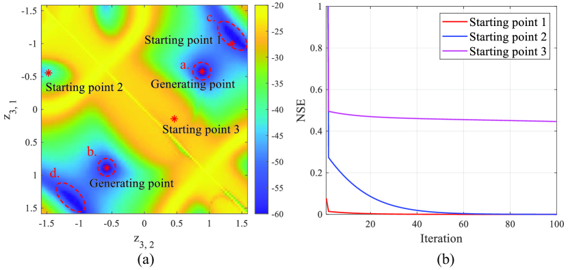
Figure 1: Iterative behaviour of ALS using different starting points of $\hat{\mathbf{z}}^{0}_{3}=[z_{3,1},z_{3,2}]^{T}$ for computing a random tensor $\boldsymbol{\mathcal{Y}}$. (a) The reconstruction NSE in dB with $K=50$ using different starting points. (b) The reconstruction NSE as a function of iteration number.

Researchers have long found in experiments that unfavorable starting points can bring CPALS into swamps [42, 27], where CPALS has not converged to a minimum and using more iterations would not further reduce the objective value. Favorable initializations not only speed up CPALS in finding a mimimum, but also can ensure the global or local convergence theoretically [43, 44]. As the initialization plays an important role for CPALS, two questions naturally arise. What are favorable initializations for CPALS? And how to generate favorable initializations? Next, we address these two questions as a way to motivate our proposed approach.

What are favorable initializations for CPALS? To answer this question, we first illustrate the iterative behaviour of CPALS using different initializations. Consider a synthetic VCP tensor $\boldsymbol{\mathcal{Y}}\in\mathbb{C}^{4\times 4\times 4}$ with $R=2$, whose factors are all Vandermonde matrices. Elements of the generating vectors are drawn from $\mathcal{U}(-\frac{\pi}{2},\frac{\pi}{2})$ randomly, which are $\mathbf{z}_{1}=[0.36,0.18]^{T}$, $\mathbf{z}_{2}=[1.10,-0.70]^{T}$ and $\mathbf{z}_{3}=[-0.58,0.89]^{T}$. Note that this tensor satisfies the uniqueness condition of Theorem 4. Here we only consider to decompose $\boldsymbol{\mathcal{Y}}$ with CPALS without calculating (9) for extracting parameters. We need to provide initializations of $\hat{\mathbf{z}}^{0}_{2}$ and $\hat{\mathbf{z}}^{0}_{3}$ to construct the initialization factors $\{\hat{\mathbf{A}}^{0}_{n}\}_{n=2}^{3}$, as shown in Algorithm 1. We use the randomly generated initialization $\hat{\mathbf{z}}^{0}_{2}=[-0.46,-0.85]^{T}$, and evaluate the performance of CPALS with different starting points of $\hat{\mathbf{z}}^{0}_{3}=[z_{3,1},z_{3,2}]^{T}$. In Figure 1 (a) and 1 (b), we show the normalized square error (NSE) calculated by $\frac{\left\|\hat{\boldsymbol{\mathcal{Y}}}-\boldsymbol{\mathcal{Y}}\right\|^{2}_{F}}{\left\|\boldsymbol{\mathcal{Y}}\right\|^{2}_{F}}$, where $\hat{\boldsymbol{\mathcal{Y}}}=\llbracket\mathbf{1}_{R};\hat{\mathbf{A}}^{K}_{1},\hat{\mathbf{A}}^{K}_{2},\hat{\mathbf{A}}^{K}_{3}\rrbracket$ is the reconstructed tensor by using CPALS. As shown in Figure 1 (a), four regions, which are surrounded by dashed circles, give favorable initializations that allow CPALS to quickly reduce the estimation error to 0. The first two regions are near the true generating point $\mathbf{z}_{3}$ and its permuted point due to permutation ambiguity. Interestingly, there are two more such regions, i.e., region c near the starting point 1 and the permuted region d. In Figure 1 (b), we plot the NSE as a function of the iteration number for CPALS by using the selected starting points. We can observe that the objective value using starting point 3 reduces slowly like in a swamp, but it reduces quickly using starting point 1. Hence, if we could define favorable initializations, then the ALS would reduce to a low objective value using just a few iterations. Note that when $\boldsymbol{\mathcal{Y}}$ is disturbed by the noise $\boldsymbol{\mathcal{N}}$, a low objective value of the approximation problem in (5), i.e., $\left\|\hat{\boldsymbol{\mathcal{Y}}}-\boldsymbol{\mathcal{Y}}-\boldsymbol{\mathcal{N}}\right\|^{2}_{F}$, may not ensure a low NSE. Nevertheless, using a small objective value as the guidance is feasible if the uniqueness condition is satisfied and the noise is small.

How to generate favorable initializations? We denote $\Psi(\boldsymbol{\mathcal{Y}})$ as a functional generator that produces initializations for CPALS to decompose $\boldsymbol{\mathcal{Y}}$. In addition to the random initialization, the most commonly used strategy is based on the SVD, i.e.,

$$\begin{split}\Psi(\boldsymbol{\mathcal{Y}}):\ &\hat{\mathbf{A}}^{0}_{n}=R\ \text{leading left singular vectors of}\ \mathbf{Y}_{(n)},\\ &\text{for }n=2,\ldots,N.\end{split}$$ (10)

However, this initialization strategy fails to consider the updating steps of CPALS in the sequel and does not ensure to generate favorable initializations. Although one can also use other non-iterative decomposition methods like the generalized eigenvalue decomposition (GEVD) to pre-estimate a starting point close to the ground truth as initialization [45], they have higher computational complexity than using the SVD. We need a $\Psi$ providing a guidance that prompts an accurate and fast CP decomposition by producing favorable initializations for the input tensor. Thus, $\Psi$ needs outer domain knowledge learned from a large number of tensor decomposition processes, which inspires us to employ a DNN.

IV-B The proposed deep-learning-aided CPALS (DL-CPALS)

We consider to develop a DNN based generator $\Psi_{\boldsymbol{\theta}}$ with parameters $\boldsymbol{\theta}$, which learns to produce favorable initial parameters to decompose new tensors fast and well. Note that the CPALS for a tensor is naturally treated as a model-driven learning task, which updates its model parameters, i.e., the CP factors, starting from the initializations. In this way, our goal is to pursue favorable initializations using a learned initialization generator $\Psi_{\boldsymbol{\theta}}$. Given a batch of CPALS tasks for decomposing tensors $\boldsymbol{\mathcal{Y}}_{1},\ldots,\boldsymbol{\mathcal{Y}}_{L_{\text{tr}}}$, we can integrate them into the data-driven learning process of $\Psi_{\boldsymbol{\theta}}$. If the unrolled CPALS is differentiable for updating the CP factors, gradients can be backpropagated to train $\Psi_{\boldsymbol{\theta}}$ for generating favorable initializations. Specifically, the loss function of the learning process is formulated as

$$\begin{split}\min_{\boldsymbol{\theta}}&\ \frac{1}{L_{\text{tr}}}\sum_{l=1}^{L_{\text{tr}}}\left\|\boldsymbol{\mathcal{Y}}_{l}-\llbracket\mathbf{1}_{R};\hat{\mathbf{A}}^{K}_{l,1},\ldots,\hat{\mathbf{A}}^{K}_{l,N}\rrbracket\right\|_{F}^{2},\\ \text{s.t.}\ &\ \{\hat{\mathbf{A}}^{0}_{l,n}\}_{n=2}^{N}=\Psi_{\boldsymbol{\theta}}(\boldsymbol{\mathcal{Y}}_{l}),\ \forall l,\\ &\ \{\hat{\mathbf{A}}^{K}_{l,n}\}_{n=1}^{N}=\Phi_{R,K}(\boldsymbol{\mathcal{Y}}_{l},\{\hat{\mathbf{A}}^{0}_{l,n}\}_{n=2}^{N}),\ \forall l.\end{split}$$ (11)

Note that the loss matches the objective function of the CP low-rank approximation problem in (5). When we set a small $K$, the proposed method aims to optimize a DNN for generating the initializations such that a small number of ALS iterations on a CP decomposition task will produce a maximally effective behavior to reduce the approximation error. Thus, the learned DNN would be a good initialization generator that can let the ALS converge to a low objective error quickly for decomposing an input tensor. Moreover, as a model-based optimization algorithm, CPALS is able to find a clean low-rank tensor from a noisy high-rank tensor by solving the low-rank approximation problem, which leads to a denoising effect. Hence, optimizing the loss function (11) and training the DNN $\Psi_{\boldsymbol{\theta}}$ does not need the paired clean data. The training data $\boldsymbol{\mathcal{Y}}_{1},\ldots,\boldsymbol{\mathcal{Y}}_{L_{\text{tr}}}$ can be noisy, which improves the practicability of the proposed method, as clean data are not available in many cases, e.g., wireless channel responses.

A prerequisite to optimize the loss function (11) is that the CPALS $\Phi_{R,K}$ is differentiable in the updated factors for all tensors. As shown in (7), the iterative updating steps of $\Phi_{R,K}$ employ a multiplication, Khatri-Rao product and pseudoinverse of matrices, where the first two are obviously differentiable. As for the pseudoinverse on the complex Hermitian matrix $\Diamond^{N}_{l\neq n}\hat{\mathbf{A}}^{T}_{l}\hat{\mathbf{A}}^{*}_{l}\in\mathbb{C}^{R\times R}$ in (7), its differential has been derived in [46], and the open source deep learning framework PyTorch [47] is able to compute gradients of the matrix pseudoinverse automatically. If $\Diamond^{N}_{l\neq n}\hat{\mathbf{A}}^{T}_{l}\hat{\mathbf{A}}^{*}_{l}$ has full rank, its pseudoinverse is equal to the inverse. Using the inverse operation can simplify the gradient calculation and make the gradient numerically stable. As we find that $\Diamond^{N}_{l\neq n}\hat{\mathbf{A}}^{T}_{l}\hat{\mathbf{A}}^{*}_{l}$ is usually full rank in experiments, we suggest using the inverse operation. The differentiable iterative updating steps of CPALS eventually leads to the learnable $\Psi_{\boldsymbol{\theta}}$.

Algorithm 2 Training of DL-CPALS

0:  the tensor dataset obeying $p(\boldsymbol{\mathcal{Y}})$, the CP rank $R$, the number of iterations $K$, the number of learning steps $I$ and the tensor mini-batch size $L$

0:  DNN $\Psi_{\boldsymbol{\theta}}$

1:  for $i=1:I$ do

2:     Draw $L$ tensors from dataset.

3:     for $l=1:L$ do

4:        Input $\boldsymbol{\mathcal{Y}}_{l}$ into $\Psi_{\boldsymbol{\theta}}$ and obtain the initialization factors $\{\hat{\mathbf{A}}^{0}_{l,n}\}_{n=2}^{N}=\Psi_{\boldsymbol{\theta}}(\boldsymbol{\mathcal{Y}}_{l})$.

5:        Carry out CPALS and obtain updated factors $\{\hat{\mathbf{A}}^{K}_{l,n}\}_{n=1}^{N}=\Phi_{R,K}(\boldsymbol{\mathcal{Y}}_{l},\{\hat{\mathbf{A}}^{0}_{l,n}\}_{n=2}^{N})$.

6:        Calculate the loss of low-rank CP approximation, i.e., $\mathcal{L}_{l}=\left\|\boldsymbol{\mathcal{Y}}_{l}-\llbracket\mathbf{1}_{R};\hat{\mathbf{A}}^{K}_{l,1},\ldots,\hat{\mathbf{A}}^{K}_{l,N}\rrbracket\right\|_{F}^{2}$

7:     end for

8:     Calculate the mini-batch-wise loss $\frac{1}{L}\sum_{l=1}^{L}\mathcal{L}_{l}$, and update $\boldsymbol{\theta}$ using optimizer.

9:  end for

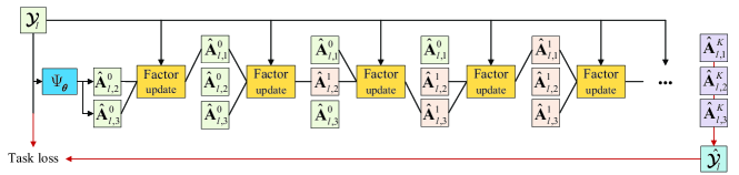
Figure 2: An illustration of the model forward propagation on a single tensor.

We provide the training steps of DL-CPALS in Algorithm 2, where we use a batch-wise training strategy. Moreover, we illustrate the forward propagation of a $3$rd order tensor in Figure 2, which corresponds to line 4 and line 5 of Algorithm 2. It can be seen that CPALS is unrolled by multiple factor updating steps using (7). As long as the factor updating steps are differentiable, the DNN parameters $\boldsymbol{\theta}$ can be optimized for learning by gradient back-propagation according to the updating loss in line 8 of Algorithm 2. After the learning terminates, one can obtain the favorable initializations by feeding the test tensor into $\Psi_{\boldsymbol{\theta}}$. Then, performing CPALS can produce an accurate decomposition solution with high efficiency.

IV-C DNN designs

In this subsection, we describe the details about the network design of the generator $\Psi_{\boldsymbol{\theta}}$. Due to the CP low-rankness assumption that $R$ is small in (11), the initializations $\{\hat{\mathbf{A}}^{0}_{l,n}\}_{n=2}^{N}$ live in a low-dimensional parameter space in comparison with the reconstructed tensor. The CPALS $\Phi_{R,K}$ uses a low-dimensional initialization to produce a low-rank approximation of the high-dimensional target tensor, which is like an explicit decoder. Thus, it is natural to design the generator $\Psi_{\boldsymbol{\theta}}$ as an encoder. In addition, $\Psi_{\boldsymbol{\theta}}$ should have a low computational complexity to compete with the SVD-based initialization. We use a simple fully connected network as generator, which outputs initial factors $\{\hat{\mathbf{A}}^{0}_{l,n}\}_{n=2}^{N}$. Note that the generator $\Psi_{\boldsymbol{\theta}}$ directly outputs the factor matrices rather than generating vectors by utilizing the Vandermonde structure, which makes the proposed method suitable for a generalized CP decomposition.

Given an input tensor $\boldsymbol{\mathcal{Y}}_{l}\in\mathbb{C}^{I_{1}\times\ldots\times I_{N}}$, we reshape it into a vector, and concatenate its real part and imaginary part into a single vector, which has dimension $2\prod_{n=1}^{N}I_{n}$. Assume that each hidden layer has $Q$ neurons. Then, the real weight matrices employed on the input layer and the hidden layer are of sizes $2\prod_{n=1}^{N}I_{n}\times Q$ and $Q\times Q$, respectively. For the output layer, the weight matrix has size of $Q\times 2R\sum_{n=2}^{N}I_{n}$. We use a Relu activation for the hidden layers. As for the activation of the output layer, we suggest to use the hyperbolic tangent function (Tanh), which constrains the output values in the interval $-1$ to $+1$ so that the energies of the initial factors are not very large and result in imbalance.

If the $\Psi_{\boldsymbol{\theta}}$ is stacked by $D$ hidden layers, considering also the biases, its total number of parameters is $2Q\prod_{n=1}^{N}I_{n}+(D-1)Q^{2}+2QR\sum_{n=2}^{N}I_{n}+DQ+2R\sum_{n=2}^{N}I_{n}$. If the input is a real tensor, the total number of parameters is $Q\prod_{n=1}^{N}I_{n}+(D-1)Q^{2}+QR\sum_{n=2}^{N}I_{n}+DQ+R\sum_{n=2}^{N}I_{n}$. In addition, in order to deal with the latent overfitting problem under limited training samples, a dropout layer is added after the activation function of each hidden layer to improve the generalization ability of the DNN model.

V Application to massive MIMO-OFDM Tensor Channel Estimation

Although the CPALS can be applied on a variety of massive MIMO systems that are not limited to those listed in Table I, we consider a representative application to MIMO-OFDM tensor channel estimation.

We first consider a downlink MIMO-OFDM system where both the mobile station (MS) and the base station (BS) are equipped with ULAs, which are of size $I_{1}$ and $I_{2}$, respectively. Suppose also that there are in total $M_{0}$ subcarriers. Consider the mmWave channel is formulated based on a geometrical model as described in [8, 48, 33]. Denote $\vartheta_{r}$ and $\theta_{r}$ as the AoA and AoD of the $r$th path, respectively. To simplify notations, we define $\Theta_{1,r}=2\pi d\sin\vartheta_{r}/\lambda$ and $\Theta_{2,r}=2\pi d\sin\theta_{r}/\lambda$ as the spatial AoA and AoD. The MIMO-OFDM channel in the spatial-frequency domain can then be written in CP form as

$$\begin{split}\boldsymbol{\mathcal{H}}_{0}=&\sum_{r=1}^{R}\beta_{r}e^{-j2\pi\frac{\tau_{r}f_{\text{s}}}{M_{0}}}\text{Van}(\Theta_{1,r})\circ\text{Van}(\Theta_{2,r})\circ\text{Van}(\frac{2\pi\tau_{r}f_{\text{s}}}{M_{0}})\\ =&\llbracket\boldsymbol{\beta};\mathbf{A}_{1},\mathbf{A}_{2},\bar{\mathbf{A}}_{3}\rrbracket\in\mathbb{C}^{I_{1}\times I_{2}\times M_{0}},\end{split}$$ (12)

where $\beta_{r}$ and $\tau_{r}$ are the equivalent path gain and delay of the $r$th path, respectively. We define $\boldsymbol{\beta}=[\beta_{1}e^{-j2\pi\frac{\tau_{1}f_{\text{s}}}{M_{0}}},\ldots,\beta_{R}e^{-j2\pi\frac{\tau_{R}f_{\text{s}}}{M_{0}}}]^{T}$. We further have $\mathbf{A}_{1}=[\text{Van}(\Theta_{1,1}),\ldots,\text{Van}_{1}(\Theta_{1,R})]\in\mathbb{C}^{I_{1}\times R}$, $\mathbf{A}_{2}=[\text{Van}_{2}(\Theta_{2,1}),\ldots,\text{Van}_{2}(\Theta_{2,R})]\in\mathbb{C}^{I_{2}\times R}$, and $\bar{\mathbf{A}}_{3}=[\text{Van}(\frac{2\pi\tau_{1}f_{\text{s}}}{M_{0}}),\ldots,\text{Van}(\frac{2\pi\tau_{R}f_{\text{s}}}{M_{0}})]\in\mathbb{C}^{M_{0}\times R}$, which are stacked by the steering vectors corresponding to the receiving ULA, transmitting ULA and subcarriers, respectively.

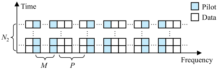
Figure 3: An illustration of the pilot pattern.

To facilitate the comparison of our method with others in experiments, we follow the pilot transmission protocol described in [33]. As the frequency correlation is helpful to improve the channel estimation accuracy, suppose that a training block has $M$ sequential subcarriers in the frequency domain to transmit $N_{2}$ training pilots in the time domain, which is illustrated in Figure 3. Two training blocks are separated by $P$ subcarriers dedicated to data transmission. We only consider the estimation of the tensor channel of a training block that corresponds to the pilot positions. Based on the pilot channels, interpolation can be used to get the data channels. The training tensor channel of a block is given by

$$\begin{split}\boldsymbol{\mathcal{H}}=[\boldsymbol{\mathcal{H}}_{0}]_{:,:,m_{\text{s}}:m_{\text{s}}+M-1}=\llbracket\boldsymbol{\beta};\mathbf{A}_{1},\mathbf{A}_{2},\mathbf{A}_{3}\rrbracket,\end{split}$$ (13)

where $m_{\text{s}}$ denotes the starting index and $\mathbf{A}_{3}$ consists of a group of $M$ rows of $\bar{\mathbf{A}}_{3}$. For the tensor channel, the BS only activates one RF chain to transmit a pilot symbol $x_{n_{2}}$ using a beamforming vector $\mathbf{f}_{2,n_{2}}\in\mathbb{C}^{I_{2}\times 1}$. During the transmission of the pilot $x_{n_{2}}$ at the BS, the MS employs $N_{1}$ combining vectors $\mathbf{f}_{1,1},\ldots,\mathbf{f}_{1,N_{1}}\in\mathbb{C}^{I_{1}\times 1}$ to process it. Note that the RF chains of the MS need to be reused when its total number is less than $N_{1}$. The channel is assumed to be block-fading, and it is constant during training. After transmitting $N_{2}$ pilots, the received baseband signal tensor can be written as

$$\begin{split}\boldsymbol{\mathcal{Y}}\!=\!\boldsymbol{\mathcal{H}}\!\times_{1}\!\mathbf{F}_{1}^{H}\!\times_{2}\text{diag}(\mathbf{x})\mathbf{F}^{T}_{2}\!+\!\boldsymbol{\mathcal{N}}\!\times_{1}\!\mathbf{F}_{1}^{H}\in\mathbb{C}^{N_{1}\!\times\!N_{2}\!\times\!M},\end{split}$$ (14)

where $\mathbf{x}=[x_{1},\ldots,x_{N_{2}}]^{T}$, $\boldsymbol{\mathcal{N}}\in\mathbb{C}^{I_{1}\times N_{2}\times M}$ is the noise tensor. $\mathbf{F}_{1}=[\mathbf{f}_{1,1},\ldots,\mathbf{f}_{1,N_{1}}]\in\mathbb{C}^{I_{1}\times N_{1}}$ and $\mathbf{F}_{2}=[\mathbf{f}_{2,1},\ldots,\mathbf{f}_{2,N_{2}}]\in\mathbb{C}^{I_{2}\times N_{2}}$ are the known combiner and beamformer, respectively. Suppose that $\mathbf{x}=\mathbf{1}_{N_{2}}$ and the rows of $\mathbf{F}_{1}$ and $\mathbf{F}_{2}$ are orthogonal with $N_{1}=I_{1}$ and $N_{2}=I_{2}$. Then, according to (13) and (14), we can obtain a coarse estimation of $\boldsymbol{\mathcal{H}}$, which is processed as

$$\begin{split}\bar{\boldsymbol{\mathcal{H}}}&=\boldsymbol{\mathcal{Y}}\times_{1}\mathbf{F}_{1}\times_{2}\mathbf{F}^{*}_{2}\\ &=\boldsymbol{\mathcal{H}}\times_{1}\mathbf{F}_{1}\mathbf{F}_{1}^{H}\times_{2}\mathbf{F}^{*}_{2}\mathbf{F}^{T}_{2}+\boldsymbol{\mathcal{N}}\times_{1}\mathbf{F}_{1}\mathbf{F}_{1}^{H}\times_{2}\mathbf{F}^{*}_{2}\\ &=\boldsymbol{\mathcal{H}}+\boldsymbol{\mathcal{N}}\times_{2}\mathbf{F}^{*}_{2}\\ &=\llbracket\boldsymbol{\beta};\mathbf{A}_{1},\mathbf{A}_{2},\mathbf{A}_{3}\rrbracket+\boldsymbol{\mathcal{N}}\times_{2}\mathbf{F}^{*}_{2}.\end{split}$$ (15)

In this way, one can collect plentiful samples at the receiver. As the least-squares-based coarse estimation can not remove the noise, the obtained a dataset of the noisy channels that characterizes a distribution $p(\bar{\boldsymbol{\mathcal{H}}})$. Fortunately, the proposed DL-CPALS can be trained by only using the noisy tensor $\bar{\boldsymbol{\mathcal{H}}}$ according to Algorithm 2. Once the model is trained, in the inference phase, the pre-estimated channel is used as input to the model $\Psi_{\boldsymbol{\theta}}$ in order to obtain favorable initialization factors. Then, the ALS with a small number of iterations is calculated to compute the estimated (denoised) channel. In addition, one can also estimate the channel parameters, such as the spatial AoAs, spatial AoDs and delays from the decomposed factors $\mathbf{A}_{1}$, $\mathbf{A}_{2}$ and $\mathbf{A}_{3}$ by solving the optimization problem (9).

VI Simulations

In this section, we evaluate the tensor CP decomposition and channel estimation performance of the proposed DL-CPALS in the considered mmWave MIMO-OFDM systems.

VI-A Results on synthetic data

We first compare the low-rank CP approximation performance of the proposed DL-CPALS with CPALS with random initializations (Random-CPALS) and CPALS with SVD-based initializations (SVD-CPALS). Consider a noisy low-rank CP tensor distribution $p(\boldsymbol{\mathcal{X}}_{\text{no}})$ with $\boldsymbol{\mathcal{X}}_{\text{no}}=\boldsymbol{\mathcal{X}}+\boldsymbol{\mathcal{N}}\in\mathbb{R}^{6\times 6\times 6}$, where the CP rank of $\boldsymbol{\mathcal{X}}$ is set as $R=3$ and $\boldsymbol{\mathcal{N}}$ is Gaussian noise. Based on the CP model of $\boldsymbol{\mathcal{X}}$ in (1), the elements of the factors $\{\mathbf{A}_{n}\in\mathbb{R}^{6\times 3}\}_{n=1}^{3}$ and the weight vector $\boldsymbol{\alpha}\in\mathbb{R}^{3\times 1}$ are all drawn from the uniform distribution $\mathcal{U}(0,1)$. Then, by setting the signal-to-noise-ratio (SNR) to $15$dB, we generate $100000$ noisy tensors of $\boldsymbol{\mathcal{X}}_{\text{no}}$, where $L_{\text{tr}}=90000$ samples are used for training and $L_{\text{te}}=10000$ samples are used for testing. For the DNN model as described in Subsection IV-C, we set the number of hidden layers to $D=4$, the number of neurons to $Q=512$ and the dropout rate to $0.3$. Thus, the total number of model parameters is $917540$. For the model training as given in Algorithm 2, the DL-CPALS uses the Adam optimizer [49] with a learning rate $0.00002$ and mini-batch size $L=512$. The number of learning steps is decided by the number of epochs, which is set to $1000$. As for the setting of the iteration number $K$, we set $K=2$ for training because using a larger $K$ does not lead to significant gains in the experiments but bring more complexity for calculating the gradients. Unless otherwise specified, $K$ is set to $50$ for testing. The performance of the competing CPALS method is evaluated from two aspects: the iterative behavior of the objective value, i.e.,

$$\begin{split}\frac{1}{L_{\text{te}}}\sum_{l=1}^{L_{\text{te}}}\left\|\boldsymbol{\mathcal{X}}_{\text{no},l}-\llbracket\mathbf{1}_{R};\hat{\mathbf{A}}^{K}_{l,1},\ldots,\hat{\mathbf{A}}^{K}_{l,N}\rrbracket\right\|^{2}_{F},\end{split}$$ (16)

and the iterative behavior of the average NSE (ANSE), i.e,

$$\begin{split}\frac{1}{L_{\text{te}}}\sum_{l=1}^{L_{\text{te}}}\frac{\left\|\boldsymbol{\mathcal{X}}_{l}-\llbracket\mathbf{1}_{R};\hat{\mathbf{A}}^{K}_{l,1},\ldots,\hat{\mathbf{A}}^{K}_{l,N}\rrbracket\right\|^{2}_{F}}{\left\|\boldsymbol{\mathcal{X}}_{l}\right\|^{2}_{F}}.\end{split}$$ (17)

In Figure 4, we first show the training loss of the proposed DL-CPALS. It can be seen that the loss value generally decreases and tends to converge as the number of epochs increases, which demonstrates that the proposed DL-CPALS is learnable. In Figure 5, we plot the performance versus number of iterations of all test samples using different initializations. Note that the elements of the initial factors for the Random-CPALS obey the uniform distribution $\mathcal{U}(0,1)$, which actually means non-negative priors are used. Figure 5(a) shows that the convergence of the proposed DL-CPALS is the steepest, because the trained model produces favorable initializations that reduce the objective value quickly. In Figure 5(b), it can be seen that the proposed method achieves the lowest reconstruction error by only using a small number of iterations (about $K=5$), while the competing Random-CPALS and SVD-CPALS fail to reach the same accuracy as DL-CPALS even with $K=50$. Based on these results, the proposed DL-CPALS leads to an accurate and fast low-rank CP decomposition.

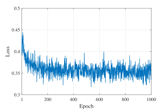
Figure 4: The training loss of DL-CPALS.

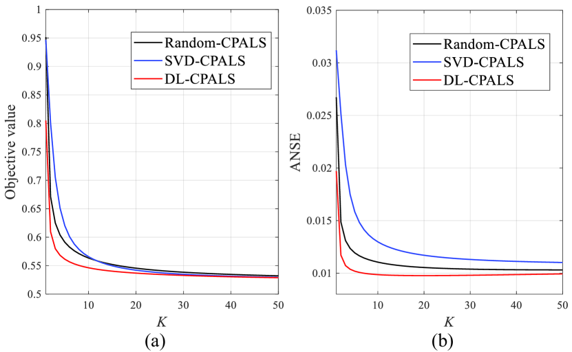
Figure 5: The performance comparison of CPALS using different initializations on synthetic data. (a) Iterative behavior of the objective value. (b) Iterative behavior of the ANSE.

VI-B Results of MIMO-OFDM channel estimation

Consider the ULAs of the MS and the BS are of size $32$ and $8$, respectively. The inter-element spacing $d$ of the ULAs is set to half the carrier wavelength $\lambda$. The sampling rate is set to $f_{\text{b}}=0.32$GHz. The total number of subcarriers is set to $M_{0}=128$, out of which a pilot block is selected randomly with $M=4$ subcarriers and $m_{\text{s}}\in\{1,\ldots,125\}$. Suppose that the elements of the noise tensor $\boldsymbol{\mathcal{N}}$ are i.i.d. $\mathcal{CN}(0,\sigma^{2})$, where $\sigma$ is determined by the SNR. The AoA $\vartheta_{r}$, AoD $\theta_{r}$, delay $\tau_{r}$ in nanoseconds and gains $\beta_{r}$ are i.i.d. with distribution $\mathcal{U}(-\frac{\pi}{2},\frac{\pi}{2})$, $\mathcal{U}(-\frac{\pi}{2},\frac{\pi}{2})$, $\mathcal{U}(0,100)$ and $\mathcal{CN}(0,1)$ for $r=1,\ldots,R$, respectively. The number of channel paths is set to $R=4$. The number of training and test samples are 90000 and 10000, respectively. The fully connected neural network structure has the setting described in Subsection VI-A, where the input layer dimension is $2I_{2}I_{1}M=2048$, and the output layer dimension is $2L(I_{1}+M)=256$. Therefore, the total number of parameters is 1886304. In order to improve the practicality of the model in actual scenarios, note that the distribution of training channel samples $p(\bar{\boldsymbol{\mathcal{H}}})$ has a mixed SNR, which is selected randomly from $\{5,10,15,20,25\}$dB.

For the proposed DL-CPALS method, a two-stage training scheme is adopted. In the first stage, we set the number of iterations $K=0$ (see Algorithm 1) and train the DNN for 1000 epochs with learning rate $0.0001$, which sets the parameters to a reasonable value range so that the reconstructed CP tensor is close to the input. Then, in the second stage, we set $K=2$ and the learning rate to $0.00002$ for training another 1000 epochs. As for the competing methods, in addition to Random-CPALS and SVD-CPALS, the supervised deep-learning-based MIMO-OFDM channel estimation method SFCNN [33] is also considered as a baseline, which uses noisy channel samples and noise-free samples to train a convolutional neural network for denoising. The SFCNN is trained for 2000 epochs with learning rate $0.001$. Other settings are the same as in the open-source codes of the paper. In addition, we also compare the competing methods with the minimum mean-squared error (MMSE) estimator. According to (14), the signal model can be written as $\mathbf{y}=\mathbf{X}\mathbf{h}+\mathbf{n}$, where $\mathbf{X}=\mathbf{I}_{M}\otimes\text{diag}(\mathbf{x})\mathbf{F}^{T}_{2}\otimes\mathbf{F}_{1}^{H}$, and $\mathbf{y}$, $\mathbf{h}$ and $\mathbf{n}$ are the vectorization forms of $\boldsymbol{\mathcal{Y}}$, $\boldsymbol{\mathcal{H}}$ and $\boldsymbol{\mathcal{N}}\!\times_{1}\!\mathbf{F}_{1}^{H}$, respectively. Then, the optimal MMSE estimation is written as $\hat{\mathbf{h}}=\hat{\mathbf{W}}\mathbf{y}$, where $\hat{\mathbf{W}}$ is given as

$$\begin{split}\hat{\mathbf{W}}=&\arg\min_{\mathbf{W}}\mathbb{E}\{\left\|\mathbf{h}-\mathbf{W}\mathbf{y}\right\|_{2}^{2}\}\\ =&\mathbb{E}\{\mathbf{h}\mathbf{h}^{H}\}\left(\mathbb{E}\{\mathbf{h}\mathbf{h}^{H}\}+\mathbb{E}\{\mathbf{n}\mathbf{n}^{H}\}\right)^{-1}\mathbf{X}^{H}.\end{split}$$ (18)

Note that the covariance matrix of the channel is estimated from all training samples and the covariance matrix of the noise is set as true according to the SNR.

Figure 6: The performance comparison of CPALS using different initializations on channel data. (a) Iterative behavior of the objective value. (b) Iterative behavior of the ANSE.

We first demonstrate the performance gain of the proposed DL-CPALS for CP decomposition on efficiency and accuracy in Figure 6, where SNR $=15$dB. Figure 6(a) shows that the proposed DL-CPALS can generate favorable initializations for the CP decomposition that make the objective function decrease rapidly. Although as $K$ increases, SVD-CPALS can achieve an objective function value similar to that of DL-CPALS, the channel estimation results of the proposed DL-CPALS are more accurate as shown in Figure 6(b).

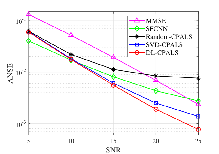
Figure 7: The ANSE of the estimated channels for different SNRs.

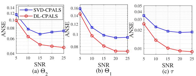
Figure 8: ANSE versus SNR of estimated channel parameters including (a) spatial AoD $\Theta_{2}$, (b) spatial AoA $\Theta_{1}$ and (c) delay $\tau$

Figure 7 shows the comparison of the channel estimation ANSE between the supervised SFCNN and the CPALS algorithm with different initializations under different SNRs with $K=50$. It can be seen that the performance of SFCNN at SNR $=5$dB is better than that of the CPALS algorithm, due to the fact that a low SNR may hurt CPALS for solving a CP low-rank approximation. Nevertheless, the performance of the proposed DL-CPALS becomes optimal as the SNR increases. Although MMSE describes a nearly optimal linear estimation performance, it cannot achieve the accuracy of the DL-CPALS that exploits the channel low-rankness. Moreover, we provide the channel parameter estimation results of SVD-CPALS and DL-CPALS in Figure 8, where the true parameters and estimated ones are all sorted in descending order due to the ambiguity. Note that the SFCNN cannot perform parameter estimation and the results of random-CPALS are poor, which is therefore not provided in the figure. It can be seen that the parameter estimation error of the proposed DL-CPALS is better than SVD-CPALS in all cases.

VI-C Complexity analysis

In this subsection, we discuss the computational complexity of the proposed DL-CPALS in the testing phase. The experiments are all implemented through Python and PyTorch programming on a single computer, which is equipped with an Intel(R) Core(TM) i7-9700K 3.60GHz CPU and 32G memory. During the testing phase, all methods are evaluated on the CPU. We consider SNR $=20$dB and focus on the channel estimation experiments of Subsection VI-B. We set the maximum number of iterations to $K=500$.

TABLE II: The number of iterations of different CPALSs for achieving the same ANSE of channel estimation

ANSE	Random-CPALS	SVD-CPALS	DL-CPALS
0.01	$36$	$5$	$2$
0.004	$259$	$15$	$5$
0.002	Fail	$158$	$36$

We report the number of iterations required for CPALS to achieve a certain channel estimation accuracy using different initialization approaches in Table II, where we can see that DL-CPALS greatly saves iterations to guarantee a certain accuracy. For example for the ANSE $=0.002$, the proposed DL-CPALS only takes 36 iterations, while SVD-CPALS takes 158 iterations and Random-CPALS fails to achieve the prescribed accuracy even after 500 iterations. Compared with Random-CPALS, both SVD-CPALS and DL-CPALS require some complexity for the initializations. According to the floating point operations (FLOPs) counter THOP of the DNN model for PyTorch, the DNN model of the proposed DL-CPALS requires 1884160 FLOPs. The storage of the DNN is 7.2 megabytes. In addition, the average initialization time of a single sample is $0.68$ milliseconds. Note that the exact number of FLOPs of the SVD-based initialization is impossible to compute as the implementation program of PyTorch is unknown, its computational complexity is on the order of $\mathcal{O}(I_{1}^{2}I_{2}M+I_{1}I_{2}M^{2})$, where $I_{1}$, $I_{2}$ and $M$ are the numbers of receiving antennas, transmitting antennas and training subcarriers, respectively. The average initialization time of a single sample is $0.57$ milliseconds. Compared with the running time it took for the ALS iterations, e.g., about $22$ milliseconds with $K=50$, the time required for computing the initializations is negligible.

VII Conclusion

This paper proposes a deep-learning-aided CP alternating least squares (DL-CPALS) method for efficient tensor CANDECOMP/PARAFAC (CP) decomposition. Specifically, by integrating the model-driven CP decomposition into the data-driven learning process, a neural network model is trained to generate favorable initializations for a fast and accurate CP decomposition. Due to the CP low-rankness constraint exploited in the model, the proposed DL-CPALS only requires noisy samples and does not require paired noise-free samples. The method is applied to the CP low-rank approximation using synthetic data and tensor channel estimation for millimeter wave multiple-input multiple-output orthogonal frequency division multiplexing (mmWave MIMO-OFDM) systems. Experimental results show that the proposed method achieves a fast and accurate CP decomposition compared with the baseline methods.

References

- [1] A. L. F. de Almeida, G. Favier, J. da Costa, and J. C. M. Mota, “Overview of tensor decompositions with applications to communications,” Signals and images: advances and results in speech, estimation, compression, recognition, filtering, and processing, pp. 325–356, 2016.
- [2] F. L. Hitchcock, “The expression of a tensor or a polyadic as a sum of products,” Journal of Mathematics and Physics, vol. 6, no. 1-4, pp. 164–189, 1927.
- [3] T. G. Kolda and B. W. Bader, “Tensor decompositions and applications,” SIAM review, vol. 51, no. 3, pp. 455–500, 2009.
- [4] H. Chen, F. Ahmad, S. Vorobyov, and F. Porikli, “Tensor decompositions in wireless communications and MIMO radar,” IEEE Journal of Selected Topics in Signal Processing, vol. 15, no. 3, pp. 438–453, 2021.
- [5] E. G. Larsson, O. Edfors, F. Tufvesson, and T. L. Marzetta, “Massive mimo for next generation wireless systems,” IEEE communications magazine, vol. 52, no. 2, pp. 186–195, 2014.
- [6] I. Barhumi, G. Leus, and M. Moonen, “Optimal training design for MIMO OFDM systems in mobile wireless channels,” IEEE Transactions on signal processing, vol. 51, no. 6, pp. 1615–1624, 2003.
- [7] H. Xie, F. Gao, and S. Jin, “An overview of low-rank channel estimation for massive MIMO systems,” IEEE Access, vol. 4, pp. 7313–7321, 2016.
- [8] Z. Zhou, J. Fang, L. Yang, H. Li, Z. Chen, and R. S. Blum, “Low-rank tensor decomposition-aided channel estimation for millimeter wave MIMO-OFDM systems,” IEEE Journal on Selected Areas in Communications, vol. 35, no. 7, pp. 1524–1538, 2017.
- [9] R. Zhang, L. Cheng, S. Wang, Y. Lou, W. Wu, and D. W. K. Ng, “Tensor decomposition-based channel estimation for hybrid mmwave massive MIMO in high-mobility scenarios,” IEEE Transactions on Communications, vol. 70, no. 9, pp. 6325–6340, 2022.
- [10] H. L. Van Trees, Optimum array processing: Part IV of detection, estimation, and modulation theory. John Wiley & Sons, 2002.
- [11] M. Sørensen and L. De Lathauwer, “Blind signal separation via tensor decomposition with Vandermonde factor: Canonical polyadic decomposition,” IEEE Transactions on Signal Processing, vol. 61, no. 22, pp. 5507–5519, 2013.
- [12] R. Roy and T. Kailath, “ESPRIT-estimation of signal parameters via rotational invariance techniques,” IEEE Transactions on Acoustics, Speech, and Signal Processing, vol. 37, no. 7, pp. 984–995, 1989.
- [13] J. Li, Z. Wu, Z. Wan, P. Zhu, D. Wang, and X. You, “Structured tensor CP decomposition-aided pilot decontamination for UAV communication in cell-free massive MIMO systems,” IEEE Communications Letters, vol. 26, no. 9, pp. 2156–2160, 2022.
- [14] J. Wang, W. Zhang, Y. Chen, Z. Liu, J. Sun, and C.-X. Wang, “Time-varying channel estimation scheme for uplink MU-MIMO in 6G systems,” IEEE Transactions on Vehicular Technology, vol. 71, no. 11, pp. 11 820–11 831, 2022.
- [15] Y. Lin, S. Jin, M. Matthaiou, and X. You, “Tensor-based channel estimation for millimeter wave MIMO-OFDM with dual-wideband effects,” IEEE Transactions on Communications, vol. 68, no. 7, pp. 4218–4232, 2020.
- [16] ——, “Channel estimation and user localization for IRS-assisted MIMO-OFDM systems,” IEEE Transactions on Wireless Communications, vol. 21, no. 4, pp. 2320–2335, 2022.
- [17] ——, “Tensor-based algebraic channel estimation for hybrid IRS-assisted MIMO-OFDM,” IEEE Transactions on Wireless Communications, vol. 20, no. 6, pp. 3770–3784, 2021.
- [18] N. D. Sidiropoulos, L. De Lathauwer, X. Fu, K. Huang, E. E. Papalexakis, and C. Faloutsos, “Tensor decomposition for signal processing and machine learning,” IEEE Transactions on Signal Processing, vol. 65, no. 13, pp. 3551–3582, 2017.
- [19] L. Sorber, M. Van Barel, and L. De Lathauwer, “Optimization-based algorithms for tensor decompositions: Canonical polyadic decomposition, decomposition in rank-(l_r,l_r,1) terms, and a new generalization,” SIAM Journal on Optimization, vol. 23, no. 2, pp. 695–720, 2013.
- [20] F. Wen, J. Shi, and Z. Zhang, “Joint 2D-DOD, 2D-DOA, and polarization angles estimation for bistatic EMVS-MIMO radar via PARAFAC analysis,” IEEE Transactions on Vehicular Technology, vol. 69, no. 2, pp. 1626–1638, 2020.
- [21] C. Qian, X. Fu, N. D. Sidiropoulos, and Y. Yang, “Tensor-based channel estimation for dual-polarized massive MIMO systems,” IEEE Transactions on Signal Processing, vol. 66, no. 24, pp. 6390–6403, 2018.
- [22] Z. Zhou, J. Fang, L. Yang, H. Li, Z. Chen, and S. Li, “Channel estimation for millimeter-wave multiuser MIMO systems via PARAFAC decomposition,” IEEE Transactions on Wireless Communications, vol. 15, no. 11, pp. 7501–7516, 2016.
- [23] J. Du, M. Han, Y. Chen, L. Jin, and F. Gao, “Tensor-based joint channel estimation and symbol detection for time-varying mmWave massive MIMO systems,” IEEE Transactions on Signal Processing, vol. 69, pp. 6251–6266, 2021.
- [24] L. Cheng, G. Yue, X. Xiong, Y. Liang, and S. Li, “Tensor decomposition-aided time-varying channel estimation for millimeter wave MIMO systems,” IEEE Wireless Communications Letters, vol. 8, no. 4, pp. 1216–1219, 2019.
- [25] G. T. de Araújo, A. L. F. de Almeida, and R. Boyer, “Channel estimation for intelligent reflecting surface assisted mimo systems: A tensor modeling approach,” IEEE Journal of Selected Topics in Signal Processing, vol. 15, no. 3, pp. 789–802, 2021.
- [26] S. Park, A. Ali, N. González-Prelcic, and R. W. Heath, “Spatial channel covariance estimation for hybrid architectures based on tensor decompositions,” IEEE Transactions on Wireless Communications, vol. 19, no. 2, pp. 1084–1097, 2020.
- [27] A. K. Smilde, P. Geladi, and R. Bro, Multi-way analysis: applications in the chemical sciences. John Wiley & Sons, 2005.
- [28] E. Sanchez and B. R. Kowalski, “Tensorial resolution: a direct trilinear decomposition,” Journal of Chemometrics, vol. 4, no. 1, pp. 29–45, 1990.
- [29] R. Bro, “Parafac. tutorial and applications,” Chemometrics and intelligent laboratory systems, vol. 38, no. 2, pp. 149–171, 1997.
- [30] H. Ye, G. Y. Li, and B.-H. Juang, “Power of deep learning for channel estimation and signal detection in OFDM systems,” IEEE Wireless Communications Letters, vol. 7, no. 1, pp. 114–117, 2017.
- [31] M. Soltani, V. Pourahmadi, A. Mirzaei, and H. Sheikhzadeh, “Deep learning-based channel estimation,” IEEE Communications Letters, vol. 23, no. 4, pp. 652–655, 2019.
- [32] H. Huang, J. Yang, H. Huang, Y. Song, and G. Gui, “Deep learning for super-resolution channel estimation and DOA estimation based massive MIMO system,” IEEE Transactions on Vehicular Technology, vol. 67, no. 9, pp. 8549–8560, 2018.
- [33] P. Dong, H. Zhang, G. Y. Li, I. S. Gaspar, and N. NaderiAlizadeh, “Deep CNN-based channel estimation for mmwave massive MIMO systems,” IEEE Journal of Selected Topics in Signal Processing, vol. 13, no. 5, pp. 989–1000, 2019.
- [34] V. Monga, Y. Li, and Y. C. Eldar, “Algorithm unrolling: Interpretable, efficient deep learning for signal and image processing,” IEEE Signal Processing Magazine, vol. 38, no. 2, pp. 18–44, 2021.
- [35] N. Shlezinger, J. Whang, Y. C. Eldar, and A. G. Dimakis, “Model-based deep learning,” Proceedings of the IEEE, pp. 1–35, 2023.
- [36] M. Borgerding, P. Schniter, and S. Rangan, “AMP-inspired deep networks for sparse linear inverse problems,” IEEE Transactions on Signal Processing, vol. 65, no. 16, pp. 4293–4308, 2017.
- [37] H. He, C.-K. Wen, S. Jin, and G. Y. Li, “Deep learning-based channel estimation for beamspace mmwave massive MIMO systems,” IEEE Wireless Communications Letters, vol. 7, no. 5, pp. 852–855, 2018.
- [38] K. Pratik, B. D. Rao, and M. Welling, “RE-MIMO: Recurrent and permutation equivariant neural MIMO detection,” IEEE Transactions on Signal Processing, vol. 69, pp. 459–473, 2021.
- [39] J. Zhang, z. Tao, L. Zhang, and Q. Zhao, “Tensor decomposition via core tensor networks,” in IEEE International Conference on Acoustics, Speech and Signal Processing (ICASSP), 2021, pp. 2130–2134.
- [40] D. Hong, T. G. Kolda, and J. A. Duersch, “Generalized canonical polyadic tensor decomposition,” SIAM Review, vol. 62, no. 1, pp. 133–163, 2020.
- [41] N. D. Sidiropoulos and R. Bro, “On the uniqueness of multilinear decomposition of n-way arrays,” Journal of Chemometrics: A Journal of the Chemometrics Society, vol. 14, no. 3, pp. 229–239, 2000.
- [42] B. C. Mitchell and D. S. Burdick, “Slowly converging PARAFAC sequences: swamps and two-factor degeneracies,” Journal of Chemometrics, vol. 8, no. 2, pp. 155–168, 1994.
- [43] A. Uschmajew, “Local convergence of the alternating least squares algorithm for canonical tensor approximation,” SIAM Journal on Matrix Analysis and Applications, vol. 33, no. 2, pp. 639–652, 2012.
- [44] L. Wang and M. T. Chu, “On the global convergence of the alternating least squares method for rank-one approximation to generic tensors,” SIAM Journal on Matrix Analysis and Applications, vol. 35, no. 3, pp. 1058–1072, 2014.
- [45] N. Vervliet, O. Debals, and L. De Lathauwer, “Tensorlab 3.0–numerical optimization strategies for large-scale constrained and coupled matrix/tensor factorization,” in 2016 50th Asilomar Conference on Signals, Systems and Computers. IEEE, 2016, pp. 1733–1738.
- [46] A. Hjorungnes and D. Gesbert, “Complex-valued matrix differentiation: Techniques and key results,” IEEE Transactions on Signal Processing, vol. 55, no. 6, pp. 2740–2746, 2007.
- [47] A. Paszke, S. Gross, F. Massa, A. Lerer, J. Bradbury, G. Chanan, T. Killeen, Z. Lin, N. Gimelshein, L. Antiga et al., “Pytorch: An imperative style, high-performance deep learning library,” Advances in neural information processing systems, vol. 32, 2019.
- [48] J. Rodríguez-Fernández, N. González-Prelcic, K. Venugopal, and R. W. Heath, “Frequency-domain compressive channel estimation for frequency-selective hybrid millimeter wave MIMO systems,” IEEE Transactions on Wireless Communications, vol. 17, no. 5, pp. 2946–2960, 2018.
- [49] D. P. Kingma and J. Ba, “Adam: A method for stochastic optimization [c],” in International Conference on Learning Representations (ICLR). San Diego, CA, USA: OpenReview.net, 2015.