The Complexity of 2-Intersection Graphs of 3-Hypergraphs Recognition for Claw-free Graphs and triangulated Claw-free Graphs

Abstract

Given a $3$-uniform hypergraph $H$, its $2$-intersection graph $G$ has for vertex set the hyperedges of $H$ and $ee^{\prime}$ is an edge of $G$ whenever $e$ and $e^{\prime}$ have exactly two common vertices in $H$. Di Marco et al. prove in [8] that deciding wether a graph $G$ is the $2$-intersection graph of a $3$-uniform hypergraph is $NP$-complete. The main problems we study concern the class of claw-free graphs. We show that the recognition problem remains $NP$-complete when $G$ is claw-free graphs but becomes polynomial if in addition $G$ is triangulated.

Keywords: uniform hypergraph, intersection graph, triangulated graph, $NP$-complete.

1 Introduction

A hypergraph $H=(V,E)$ [1] is a generalization of the concept of graph. In detail, it is defined considering a set of vertices $V=\{v_{1},\ldots,v_{n}\}$ and a set $E\subset 2^{|V|}\setminus\{\emptyset\}$ of hyperedges such that $e\not\subset e^{\prime}$ for any pair $e,e^{\prime}$ of $E$. In the case in which $|e|=1,\forall e\in E$ we say that $H$ is trivial.

Similarly to the graph case, the degree of a vertex $v\in V$ is the number of hyperedges $e\in E$ such that $v\in e$. Another important notion in the field of hypergraphs is that of uniformity. We say that $H$ is $k$-uniform if $|e|=k$ for all hyperedge $e\in E$. We also suppose that $H$ has no parallel hyperedges, i.e., $e\neq e^{\prime}$ for any pair $e,e^{\prime}$ of hyperedges. Therefore, a simple graph (loopless and without parallel edges), is a $2$-uniform hypergraph.

In this paper we are concerned with the reconstruction of intersection graphs of hypergraphs. In particular, given a $k$-uniform hypergraph $H$, its $l$-intersection graph $G=L_{k}^{l}(H),1\leq l<k$ is $G=(E,F)$ where the vertex set is $E$, and $ee^{\prime}\in F$ if and only if $|e\cap e^{\prime}|=l$ (i.e. two hyperedges of $H$ intersect by exactly $l$ elements). Note that a similar definition could be given for general hypergraphs. However, here we focus only on the simpler uniform case.

Starting from the previous idea, new concepts could be introduced. For example, given a pair of vertices $u,v\in H$, their multiplicity is the number of edges in $H$ containing both $u$ and $v$. We denote with $m(H)$ the maximum multiplicity among all pairs of vertices. From this notion follows the concept of linear hypergraphs. In particular, $H$ is linear if and only if $m(H)=1$.

In general, we define $L_{k}^{l}$ as the class of graphs $G$ such that there exists a $k$-uniform hypergraph $H$ such that $G=L_{k}^{l}(H)$. In such a case we say that $H$ is a preimage of $G$ (note that a preimage is not necessarily unique). In particular, note that $L_{2}^{1}$ corresponds to the class of line graph. Finally, we denote $L_{k}^{\infty}=\bigcup_{i=1}^{k-1}L_{k}^{i}$.

Since we are interested in finding when a graph has a preimage, we use specific labelling to label each vertex of $G$ appropriately. In particular, for $G=L_{k}^{l}(H)$ a $\lambda_{k}^{l}$-labelling is a labelling of its vertices such that the label of a vertex $e$ is a $k$-set

Some previous results are proved in the literature about intersection graphs. In particular in [11], Hlinĕný and Kratochvíl proved that deciding whether a graph $G$ belongs in $L_{3}^{1}$ is $NP$-complete. On the other hand, from the characterization of line graphs by Beineke [2] the problem of deciding whether $G$ belongs in $L_{2}^{1}$ is polynomial.

In [8] Di Marco et al. are interested in the null label problem on hypergraphs and in the reconstruction of graphs in $L_{3}^{2}$. In particular, in a previous paper, they prove a sufficient condition about the existence of the former [7] using graphs in that family. Finally, they also proved that the problem of deciding whether a graph $G$ belongs in $L_{3}^{2}$ is $NP$-complete.

In this work, relying on that result, we are interested in studying some subclasses of $L_{3}^{2}$ in which the problem could be polynomial solvable. In fact, one can remark that a graph $G\in L_{3}^{2}$ is $K_{1,4}$-free. A natural subclass of $K_{1,4}$-free graph is the set of claw-free graphs, thus we are interested in the characterization of them in $L_{3}^{2}$. In particular, here we show that deciding whether a claw-free graph belongs to $L_{3}^{2}$ remains a $NP$-complete problem, but, interestingly, it is polynomial in the subclass of triangulated graphs.

The article is organized as follows. In Section 2 we give the notation and definition of graph theory we use throughout the paper, focusing also on properties of the class $L_{3}^{2}$. In section 3 we study the reconstruction of the subclasses of claw-free and triangulated graphs. Finally, in Section 4, we give some properties and complexity results for the graphs in $L_{k}^{l}$.

2 Graphs definitions and notations

In this section we provide some basic definitions, used throughout the paper. The reader is referred to [5] for definitions and notations in graph theory.

We are concerned with simple undirected graphs $G=(V,E)$, $|V|=n,|E|=m$. For $v\in V$, we define the open neighbourhood $N(v)=\{w\in V\ |\ (v,w)\in E\}$. Similarly, we define $N[v]=N(v)\cup\{v\}$ its closed neighbourhood. The degree of $v\in V$ is $d_{G}(v)=|N(v)|$ or simply $d(v)$ when the context is unambiguous. We denote with $\Delta(G),\delta(G)$ the maximal, respectively minimal, degree of a vertex. A vertex $v$ is universal if $N[v]=V$. A vertex $v$ is a leaf if $d(v)=1$. $G$ is $k$-regular when $d(v)=k$ for any $v\in V$.

For $S\subseteq V$, let $G[S]$ denote the subgraph of $G$ induced by $S$, which has vertex set $S$ and edge set $\{uv\in E\;|\;u,v\in S\}$. For $v\in V$, we write $G-v=G[V\setminus\{v\}]$. Similarly, for $S\subsetneq V$ and $v\in V\setminus S$ we write $G[S]+v=G[S\cup\{v\}]$. For $e\in E$, we write $G-e=(V,E\setminus\{e\})$.

For $k\geq 1$, $P_{k}=u_{1}-u_{2}-\cdots-u_{k}$ is a chordless path if no two vertices are connected by an edge that is not in $P_{k}$, i.e. if $V_{P_{k}}=\{u_{1},\ldots,u_{k}\}$ then $G(V_{P_{k}})=P_{k}$. In a similar fashion, it is possible to define a chordless cycle $C_{k}=u_{1}-u_{2}-\cdots-u_{k}-u_{1}$ for $k\geq 3$. For $k\geq 4$, $C_{k}$ is called a hole. A graph without a hole is chordal or, equivalently, triangulated.

We say that $S\subseteq V$ is called a clique if $G[S]$ is a complete graph, i.e., every pairwise distinct vertices $u,v\in S$ are adjacent. We denote with $K_{p}$ the clique on $p$ vertices and we say that $C_{3}=K_{3}$ is a triangle. $K_{1,p}$ is the star on $p+1$ vertices, that is, the graph with vertices $\{u,v_{1},v_{2}\ldots,v_{p}\}$ and edges $uv_{1},uv_{2},\cdots,uv_{p}$. $K_{1,3}$ is a claw.

For $S\subset V$ the clique $G[S]$ is maximal if for any $v\in V\setminus S$ then $G[S]+v$ is not a clique. When the context is unambiguous a clique will be always a maximal clique. In this paper a clique $K$ is small, medium, big when $|K|\leq 2,3\leq|K|\leq 4,|K|\geq 5$, respectively.

A cut-edge in a connected graph $G$ is an edge $e\in E$ such that $G-e$ is not connected.

For a fixed graph $H$ we write $H\subseteq G$ whenever $G$ contains an induced subgraph isomorphic to $H$. Instead, $G$ is $H$-free if $G$ has no induced subgraph isomorphic to $H$.

2.1 Properties of graphs in $L_{3}^{2}$

When dealing with reconstruction issues on graphs, it is important to consider the maximal cliques. For such reason, provided $G\in L_{3}^{2}$, we give some properties involving its maximal cliques.

Let $K_{3}$, the triangle $T=K_{3}$ with vertices $a,b,c$. Two cases can be detected following from two different hyperedges configurations in the related $3$-uniform hypergraph: either $a=\{1,2,x\},b=\{1,2,y\},c=\{1,2,z\},x\neq y\neq z$ or $a=\{1,2,3\},b=\{1,2,4\},c=\{1,3,4\}$. The first case is defined as positive clique and the second negative clique.

A similar situation occurs with $K_{4}$. In fact, if we consider a clique with four vertices $a,b,c,d$, then again two cases appear: either $a=\{1,2,x\},b=\{1,2,y\},c=\{1,2,z\},d=\{1,2,t\},x\neq y\neq z\neq t$ or $a=\{1,2,3\},b=\{1,2,4\},c=\{1,3,4\},d=\{2,3,4\}$. The first case is denoted as positive clique and the second negative clique.

For bigger cliques, the situation is easier. Let $K_{p},p\geq 5,$ the clique with $p$ vertices $a_{1},\ldots,a_{p}$. Then it must be $a_{i}=\{1,2,x_{i}\},1\leq i\leq p$. We defined all these cases as positive. Note that, in general, we are referring to positive cliques whenever their labels are composed of only one sharing couple. The other cases are referred to as negative.

To set the notation, when a clique $K$ is positive we denote it by $K^{+}$ and $K^{-}$ otherwise. For convenience the clique of two vertices $K_{2}$ is both positive and negative.

Property 2.1

If $K_{i},K_{j}$ are two cliques such that $|K_{i}\cap K_{j}|=2$ then we have $K_{i}^{+}$ and $K_{j}^{-}$ (or vice versa).

Proof:  W.l.o.g. let us consider $K_{i}\cap K_{j}=\{u,v\}$ with $u=\{1,2,3\},v=\{1,2,4\}$ and $s\in K_{i}\setminus K_{j},t\in K_{j}\setminus K_{i}$ be such that $st\not\in E$. For contradiction, we assume that $K_{i}^{+},K_{j}^{+}$ or $K_{i}^{-},K_{j}^{-}$. Two cases arises: if $K_{i}^{+},K_{j}^{+}$, then it holds $s=\{1,2,5\},t=\{1,2,6\}$ that is not possible. Lastly, if $K_{i}^{-},K_{j}^{-}$, then w.l.o.g., it holds $s=\{1,3,4\}$, again a contradiction when labelling $t$.    $\Box$

A simple consequence of the previous Property is the following.

Corollary 2.1

Let $e$ be an edge of $G\in L_{3}^{2}$. Then $e$ is an edge of at most two cliques.

Also the following proposition holds.

Property 2.2

Let $K_{n},K_{m}$ be two distinct cliques of $G=(V,E)\in L_{3}^{2}$. Then $|K_{n}\cap K_{m}|\leq 2$.

Proof:  For contradiction, assume that $K_{n}\cap K_{m}\supseteq\{x,y,z\}$. There exists $v_{1}\in K_{n}\setminus K_{n}\cap K_{m},v_{2}\in K_{m}\setminus K_{n}\cap K_{m}$ such that $v_{1}v_{2}\not\in E$.

If one of the two cliques, say $K_{n}$, is positive then $x=\{1,2,3\},y=\{1,2,4\},z=\{1,2,5\}$. Thus $v_{1}=\{1,2,6\},v_{2}=\{1,2,7\}$, a contradiction.

Therefore, consider $K_{n}=K_{4}^{-},i=1,2$. Thus, $x=\{1,2,3\},y=\{1,2,4\},z=\{1,3,4\}$ but $v_{1}=\{2,3,4\},v_{2}=\{2,3,4\}$, another contradiction.    $\Box$

Based on that, for two (maximal) cliques $K_{i},K_{j}$ we say that they are strongly intersecting when $|K_{i}\cap K_{j}|=2$ and they are weakly intersecting when $|K_{i}\cap K_{j}|=1$.

3 Reconstruction of claw-free graphs in $L_{3}^{2}$

In this section we deal with the recognition of claw-free graphs in $L_{3}^{2}$. We initially show that there exist claw-free graphs in $L_{3}^{2}$ and then we provide some necessary conditions to check the belonging. However, we prove that, in general, the recognition problem is $NP$-complete for that class.

3.1 Claw-free graphs in $L_{3}^{2}$

Figure 2 shows a claw-free graph belonging to $L_{3}^{2}$. This is not always the case, as witnessed by Figure 1. In fact, using Proposition 2.2 it directly follows that the graph $K_{5}-e$ has no realization.

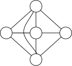
Figure 1: $K_{5}-e$ has no realization.

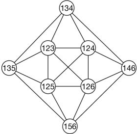
Figure 2: A graph in $L_{3}^{2}$.

We now show some examples of claw-free graphs in $L_{3}^{2}$ that will be used in the following proofs.

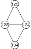
Figure 3: A realization of the diamond.

Corollary 3.1

If $G\in L_{3}^{2}$ contains, as an induced subgraph, a diamond $D$ consisting of the two triangles $T_{1},T_{2}$ then we have either $T_{1}^{-},T_{2}^{+}$ or $T_{1}^{+},T_{2}^{-}$.

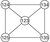
Figure 4: A realization of the $4$-wheel $W_{4}$.

Corollary 3.2

If $G\in L_{3}^{2}$ contains, as an induced subgraph, a $4$-wheel $W_{4}$ consisting of the four triangles $T_{1}=\{a,b,c\},T_{2}=\{a,c,d\},T_{3}=\{a,d,e\},T_{4}=\{a,b,e\}$ then we have either $T_{1}^{-},T_{2}^{+},T_{3}^{-},T_{4}^{+}$ or $T_{1}^{+},T_{2}^{-},T_{3}^{+},T_{4}^{-}$.

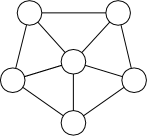
Figure 5: The $5$-wheel $W_{5}$.

Corollary 3.3

If $G\in L_{3}^{2}$ then it cannot contains the $5$-wheel $W_{5}$ as an induced subgraph.

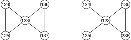
Figure 6: Two realizations of the butterfly.

Property 3.1

If $G\in L_{3}^{2}$ contains, as an induced subgraph, a butterfly $B$ consisting of the two triangles $T_{1},T_{2}$ then we have either $T_{1}^{+},T_{2}^{+}$ or $T_{1}^{-},T_{2}^{+}$ or $T_{1}^{+},T_{2}^{-}$.

Proof:  Let $T_{1}=\{a,b,c\},T_{2}=\{a,d,e\}$. The figure 6 shows two realizations with $T_{1}^{+},T_{2}^{+}$ or $T_{1}^{-},T_{2}^{+}$ or $T_{1}^{+},T_{2}^{-}$. It remains to show that $T_{1}^{-},T_{2}^{-}$ is impossible. Let $a=\{1,2,3\},b=\{1,2,4\},c=\{1,3,4\}$. We have $d=\{2,3,5\}$ but is not possible to label $T_{2}$ in such a way it is negative.    $\Box$

The prism $P$ consists of two vertex disjoint triangles $T_{1}=\{a,b,c\},T_{2}=\{d,e,f\}$ plus the three edges $ad,be,cf$.

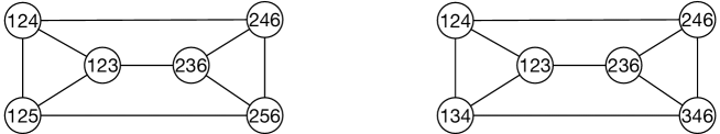
Figure 7: Two realizations of the prism.

Fact 3.1

If $G\in L_{3}^{2}$ contains, as an induced subgraph, a prism $P$ then we have $T_{1}^{+},T_{2}^{+}$ or $T_{1}^{-},T_{2}^{-}$.

Proof:  For contradiction, assume that $T_{1}^{+},T_{2}^{-}$. Let $a=\{1,2,3\},b=\{1,2,4\},c=\{1,2,5\}$. Without loss of generality $d=\{1,3,6\}$. Then we have $e=\{1,6,4\}$. It follows that $f=\{1,5,6\}$, so $T_{2}$ is positive, a contradiction.    $\Box$

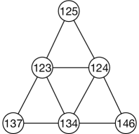
Figure 8: A realization of the sun $S_{3}$.

Fact 3.2

If $G\in L_{3}^{2}$ contains, as an induced subgraph, a sun $S_{3}$ consisting of the four triangles $T_{1}=\{a,b,c\},T_{2}=\{a,b,d\},T_{3}=\{a,c,e\},T_{4}=\{b,c,f\}$ then we have $T_{1}^{-},T_{2}^{+},T_{3}^{+},T_{4}^{+}$ with $a=\{1,2,3\},b=\{1,2,4\},c=\{1,3,4\},d=\{1,2,5\},e=\{1,3,6\},f=\{1,4,7\}$.

Proof:  From Corollary 2.1 we have either $T_{1}^{-},T_{2}^{+},T_{3}^{+},T_{4}^{+}$ or $T_{1}^{+},T_{2}^{-},T_{3}^{-},T_{4}^{-}$. The figure 8 shows a realization with $T_{1}^{-},T_{2}^{+},T_{3}^{+},T_{4}^{+}$. Now we assume that $T_{1}^{+},T_{2}^{-},T_{3}^{-},T_{4}^{-}$ with $a=\{1,2,3\},b=\{1,2,4\},c=\{1,2,5\}$. Then, w.l.o.g., $d=\{1,3,4\}$. It follows that $e=\{2,4,5\}$ but $f$ cannot be labelled.    $\Box$

Fact 3.3

If $G\in L_{3}^{2}$ contains, as an induced subgraph, a path on three vertices $u-v-w$ with $u=\{a,b,c\},w=\{d,e,f\}$ then $\{a,b,c\}\cap\{d,e,f\}\neq\emptyset$.

As mentioned before, we denote with $K_{4}+v$ is the graph with five vertices $\{a,b,c,d,e\}$ where $\{a,b,c,d\}$ is complete and $e$ is connected to exactly one vertex, say $a$.

Fact 3.4

If $G\in L_{3}^{2}$ contains $K_{4}+v$, as an induced subgraph, then the clique $K_{4}$ of $K_{4}+v$ is positive.

Proof:  For contradiction, assume that the clique on four vertices $G[\{a,b,c,d\}]$ is negative: $a=\{1,2,3\},b=\{1,2,4\},c=\{1,3,4\},d=\{2,3,4\}$. Then, without loss of generality, $e=\{1,2,5\}$. So $be\in E$, a contradiction.    $\Box$

Note that all the graphs we have considered in this subsection are claw-free.

3.2 Recognition for claw-free graphs in $L_{3}^{2}$

In [8] authors prove that recognizing whether a graph $G$ is in $L_{3}^{2}$ is $NP$-complete. Since a graph in $L_{3}^{2}$ is $K_{1,4}$-free we are concerned with the subclass of claw-free graphs ($K_{1,3}$-free graphs).

We will prove that the problem of deciding if $G\in L_{3}^{2}$ is $NP$-complete. To reach our goal we need an intermediate problem that is defined and proved $NP$-complete below.

The $2$-labelling intersection ($2LI$) problem

Let us consider a simple graph $G=(V,E)$ and a partition of its edge-set $E$ into two subsets $E_{w}$ and $E_{s}$, i.e. $E=E_{w}\cup E_{s}$ and $E_{w}\cap E_{s}=\emptyset$. We call weak edges the edges in $E_{w}$ and strong edges those in $E_{s}$.

We define a function $\varphi$, say a $2$-labelling, that associates to each vertex $v\in V$ a pair of labels $\{a_{v},b_{v}\}$ such that:

$i)$ if $v_{1}\neq v_{2}$, then $\varphi(v_{1})\neq\varphi(v_{2})$;

$ii)$ if $v_{1}v_{2}\in E_{w}$, then $\varphi(v_{1})\cap\varphi(v_{2})=\emptyset$;

$iii)$ if $v_{1}v_{2}\in E_{s}$, then $|\varphi(v_{1})\cap\varphi(v_{2})|=1$.

See Fig.9 for an example.

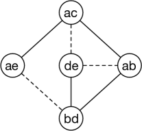
Figure 9: A graph with a $2$-labelling $\varphi$. Weak and strong edges are represented by dotted and straight lines, respectively, while the nodes show the pair of elements associated by $\varphi$.

The $2LI$ problem, provided in its decision form, follows

$2$-labelling intersection ($2LI$)     Instance: a simple graph $G=(V,E)$ and a partition of its edges into $E_{w}$ and $E_{s}$. Question: does $G$ admit $\varphi$ a $2$-labelling of its vertices?

We show the NP-completeness of $2LI$ by a reduction that involves the problem $3-SAT$ (LO2 in [9])

$3$-SAT     Instance: a set $U$ of variables, a collection $C$ of clauses over $U$ such that each clause $c\in C$ has $|c|=3$. Question: Is there a satisfying truth assignment for $C$?

Given an instance $A$ of $3$-Sat, we construct a graph $G_{A}=(V_{A},E_{A})$ and a partition of its edges into weak and strong edges $E_{A,w}$ and $E_{A,s}$ such that the $3$-Sat instance admits a solution if and only if $G_{A}$ admits a $2$-labelling. This will imply the NP-completeness of $2LI$.

Hence, we start by providing two graphs’ prototypes to model variables and clauses of the $3$-Sat instance $A$, then we show how to use them to reach the graph $G_{A}$.

Representing the variables and the clauses of $A$

Let us define the graph $G_{x}=(V_{x},E_{x})$ that will be used to represent each variable $x\in U$. The set $V_{x}$ consists of three vertices $v_{1}^{x}$, $v_{2}^{x}$, and $v_{3}^{x}$, while $E_{x}$ is partitioned into the weak edges $E_{x,w}=\{v_{2}^{x}v_{3}^{x}\}$ and the strong edges $E_{x,s}=\{v_{1}^{x}v_{2}^{x},v_{1}^{x}v_{2}^{x}\}$ (see Fig.10, $(a)$).

Figure 10: $(a)$ the graph defined for a variable $x\in U$; (b) the graph defined for a clause $c\in C$. In $(a)$ the nodes show the pair of elements associated by $\varphi$.

Lemma 3.4

Let $G_{x}$ be the graph related to variable $x$ and $\varphi(v_{1}^{x})=\{a,b\}$. It holds, w.l.o.g., that $a\in\varphi(v_{2}^{x})$ and $b\in\varphi(v_{3}^{x})$.

The proof is immediate by definition of weak and strong edges.

The gadget $G_{x}$ will also be used to represent the dichotomy of the truth values in the final graph. In particular, from now on, we consider the truth values labels $T$ and $F$. We define $G_{TF}$ similarly to $G_{x}$ with the further assumption that $a=T$ and $b=F$.

On the other hand, we associate to each clause $c\in C$ a graph $G_{c}=(V_{c},E_{c})$ having five vertices $V_{c}=\{v_{c}^{1},v_{c}^{2},v_{c}^{3},v_{c}^{4},v_{c}^{5}\}$ and four strong connections, i.e., $E_{c}=E_{c,s}=\{v_{c}^{1}v_{c}^{4},v_{c}^{2}v_{c}^{4},v_{c}^{3}v_{c}^{5},v_{c}^{4}v_{c}^{5}\}$ (see Fig.10, $(b)$).

Putting things together

So, starting from an instance $A$ of $3$-Sat, we proceed in defining the graph $G_{A}=(V_{A},E_{A})$. The reader can follow the construction in Fig.11. We include in $G_{A}$ $n=|U|$ graphs $G_{x_{1}},\dots,G_{x_{n}}$ representing the variables of $U$, $m=|C|$ graphs $G_{c_{1}},\dots,G_{c_{m}}$ representing the clauses of $C$, and the graph $G_{TF}$.

The connections between these graphs in $G_{A}$ are set according to the following rules:

$(1)$ the variables are connected by all the possible weak edges between the vertices $v_{x}^{1}$, i.e., for each couple of variable $x$ and $y$ in $U$, we set the weak edge $v_{x}^{1}v_{y}^{1}\in E_{A,w}$;

$(2)$ let $x$ be the $i$-th variable involved in the clause $c$, with $1\leq i\leq 3$. We set the weak edge $v_{x}^{1}v_{c}^{i}\in E_{A,w}$, and the strong edge $v_{x}^{3}v_{c}^{i}\in E_{A,s}$ if $x$ is negated, $v_{x}^{2}v_{c}^{i}\in E_{A,s}$ otherwise;

$(3)$ for each variable $x$, we set the strong edges $v_{x}^{2}v^{1}_{TF},v^{3}_{x}v^{1}_{TF}\in E_{A,s}$ to connect the variable to the truth values in $G_{TF}$. Furthermore, we set three more strong edges $v^{4}_{c}v^{1}_{TF},v^{5}_{c}v^{1}_{TF},v^{5}_{c}v^{2}_{TF}\in E_{A,s}$ to connect also each clause $c$ to the truth values in $G_{TF}$.

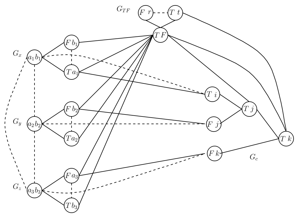
Figure 11: The graph $G_{A}$ for a clause $C={\bar{x}}\vee y\vee z$

Theorem 3.5

Given an instance $A$ of $3$-Sat, the graph $G_{A}$ admits a $2$-labelling if and only if the instance $A$ has a solution.

Proof:  Suppose that a $2$-labelling $\varphi$ exists. Let $\{a_{i},b_{i}\}$ be the label associated to the node $v^{1}_{x_{i}}$ of $G_{x_{i}}$. The connections in $(1)$ assure that the labels $\{a_{i},b_{i}\},1\leq i\leq n,$ have no common elements.

By the edges in $(2)$, for each variable $x$, one among $v^{1}_{x}$ and $v^{2}_{x}$ contains $T$, while $F$ belongs to the other since their labels can not intersect by definition of $G_{x}$. Let us consider a clause $c$ involving literals of the (distinct) variables $x$, $y$ and $z$. $\varphi(v_{c}^{1})$ contains, by the edges in $(2)$, the truth value either in $\varphi(v_{x}^{2})$ or in $\varphi(v_{x}^{3})$ of $G_{x}$ to whom it is strongly connected. Note that $\varphi(v_{c}^{1})$ and $\varphi(v_{x}^{1})$ does not intersect since a weak edge is set between them in $(2)$.

Now, consider the node $v_{c}^{4}$: it is strongly connected both with $v^{1}_{TF}$, $v_{c}^{1}$, and $v_{c}^{2}$, so its label contains $T$ or $F$ according to the values of $\varphi(v_{c}^{1})$ and $\varphi(v_{c}^{2})$. More precisely, the following three cases arise:

- $T\in\varphi(v_{c}^{1})$ and $T\in\varphi(v_{c}^{2})$: it follows that $T\in\varphi(v_{c}^{4})$;

- $T\in\varphi(v_{c}^{1})$ and $F\in\varphi(v_{c}^{2})$, or conversely: it follows that one among $T$ or $F$, but not both, belongs to $\varphi(v_{c}^{4})$;

- $F\in\varphi(v_{c}^{1})$ and $F\in\varphi(v_{c}^{2})$: it follows that $F\in\varphi(v_{c}^{4})$.

Finally, consider the node $v_{c}^{5}$: since it is strongly connected to $v^{1}_{TF}$ and $v^{2}_{TF}$, its label contains, w.l.o.g. $T$. By the three cases above, if $T\in\varphi(v_{c}^{5})$, then it holds $T\in\varphi(v_{c}^{3})$ or $T\in\varphi(v_{c}^{4})$. So, $F\in\varphi(v_{c}^{1})$, $F\in\varphi(v_{c}^{2})$, and $F\in\varphi(v_{c}^{3})$ if and only if $G_{c}$ does not admit a $2$-labelling, and the same holds for $G_{A}$. Since the three truth values in $\varphi(v_{c}^{1})$, $\varphi(v_{c}^{2})$, and $\varphi(v_{c}^{3})$ are the truth values of the literals in $c$, then a truth assignment for $c$ exists if and only if a $2$-labelling for $G_{c}$ does.

It is clear that the converse holds, as the construction is reversible.    $\Box$

Theorem 3.6

Let $G=(V,E)$ be a claw-free graph. Deciding whether there exists a $3$-uniform hypergraph $H$ such that $G=L_{3}^{2}(H)$ is a $NP$-complete problem.

Proof:  The proof has two parts. Firstly, we define $\cal C$ a subclass of claw-free graphs we are interested here. Then we show that the problem of deciding wether $G\in\cal C$ is such that $G\in L_{3}^{2}$ is equivalent to the problem $2LI$ which is $NP$-complete from Theorem 3.5.

First: the definition of $\cal C$. A graph $G\in\cal C$ consists of components $C_{1},\ldots,C_{k}$ each of the $C_{i}$’s being a clique of size at least five, the $C_{i}$’s form a partition of the vertex set of $G$. When two components $C_{i},C_{j}$ are linked there are connected by either a strong link or a weak link. A strong link consists of a $C_{4}$ of $G$ with its two non adjacent vertices $i_{1},i_{2}\in C_{i}$ and its two other non adjacent vertices $j_{1},j_{2}\in C_{j}$. A weak link consist of a $K_{4}$ of $G$ with two vertices $i_{1},i_{2}\in C_{i}$ and the two other vertices $j_{1},j_{2}\in C_{j}$. The links, weak or strong, have no common vertices. It follows that $G$ is claw-free. Moreover, since $|C_{i}|\geq 5$, $C_{i}\cup C_{j}$ the union of two distinct components cannot be a clique.

When $G\in L_{3}^{2}$ the components satisfy the following: Since each component $C_{i}=\{v_{1}^{i},v_{2}^{i},\ldots,v_{p}^{i}\}$ has at least five vertices, we necessarily have $v_{1}^{i}=\{i,i^{\prime},1\},v_{2}^{i}=\{i,i^{\prime},2\},\ldots,v_{p}^{i}=\{i,i^{\prime},p\}$ and $C_{i}$ is associated with its pair of common labels $\{i,i^{\prime}\}$. For two distinct components $C_{i},C_{j}$ we have $|\{i,i^{\prime}\}\cap\{j,j^{\prime}\}|\leq 1$. When $C_{i},C_{j}$ are connected with a strong link then we have $|\{i,i^{\prime}\}\cap\{j,j^{\prime}\}|=1$. When $C_{i},C_{j}$ are connected with a weak link then we have $\{i,i^{\prime}\}\cap\{j,j^{\prime}\}=\emptyset$.

Second: equivalence with the problem $2LI$. Given $G\in\cal C$ we define the graph $G^{\prime}$ as follows: to the vertices $v_{i}$ of $G^{\prime}$ correspond the components $C_{i}$ of $G$, and vice versa; to a strong (resp. weak) link of $G$ corresponds a strong (resp. weak) edge of $G^{\prime}$, and vice versa.

We assume that there exists a $3$-uniform hypergraph $H$ such that $G=L_{3}^{2}(H)$. Since $|C_{i}|\geq 5$ the intersection of the labels of the pairs of vertices in the same component $C_{i}$ is the same two labels says $\{i,i^{\prime}\}$. Now, for two distinct $C_{i},C_{j}$, since $C_{i}\cup C_{j}$ is not a clique we have that $|\{i,i^{\prime}\}\cap\{j,j^{\prime}\}|\leq 1$. When $C_{i},C_{j}$ are strongly connected then $|\{i,i^{\prime}\}\cap\{j,j^{\prime}\}|=1$, when they are weakly connected then $|\{i,i^{\prime}\}\cap\{j,j^{\prime}\}|=0$. Thus for each vertex $v_{i}$ of $G^{\prime}$ when assigning the two labels $i,i$ to $v_{i}$ we obtain a positive answer for the problem $2LI$.

Now, we assume that the problem $2LI$ has a positive answer. Let $i,i^{\prime}$ be the two labels assigned to $v_{i}$ in $G^{\prime}$. We assign $\{i,i^{\prime}\}$ to the component $C_{i}$ of $G$. Let $v_{i},v_{j}$ be two vertices linked with a strong edge. Then the labels associated to $C_{i},C_{j}$ are $\{i,i^{\prime}\},\{i,j\}$, respectively. Let $w_{1}^{i},w_{2}^{i}$ and $w_{1}^{j},w_{2}^{j}$ be respectively the two vertices of the strong link between $C_{i}$ and $C_{j}$. Then $w_{1}^{i}=\{i,i^{\prime},a\},w_{2}^{i}=\{i,i^{\prime},b\},w_{1}^{j}=\{i,j,a\},w_{2}^{j}=\{i,j,b\}$. Let $v_{i},v_{j}$ be two vertices linked with a weak edge. Then the labels associated to $C_{i},C_{j}$ are $\{i,i^{\prime}\},\{j,j^{\prime}\}$, respectively. Let $w_{1}^{i},w_{2}^{i}$ and $w_{1}^{j},w_{2}^{j}$ be respectively the two vertices of the weak link between $C_{i}$ and $C_{j}$. Then $w_{1}^{i}=\{i,i^{\prime},j\},w_{2}^{i}=\{i,i^{\prime},j^{\prime}\},w_{1}^{j}=\{j,j^{\prime},i\},w_{2}^{j}=\{j,j^{\prime},i^{\prime}\}$. Thereafter, when a vertex $w_{k}^{i}\in C_{i}$ is not contained in a link, weak or strong, we take $w_{k}^{i}=\{i,i^{\prime},k\}$. Thus there exists $H$ a $3$-uniform hypergraph $H$ such that $G=L_{3}^{2}(H)$.    $\Box$

3.3 Recognition for triangulated claw-free graphs in $L_{3}^{2}$

Recall that a graph $G$ is triangulated (or chordal) if it is $C_{k}$-free, $k\geq 4$.

It is known that to each triangulated graph $G=(V,E)$, we can associate, in linear time [4], a maximal clique tree $T=(C,S)$ where each maximal clique of $G$ corresponds to a vertex $c\in C$ and $cc^{\prime}\in S$ if $c\cap c^{\prime}\neq\emptyset$ and $c\cap c^{\prime}$ is a minimal separator of $G$ which is a clique. An example is shown in Figure 12

Figure 12: Example of a claw-free triangulated graph and its associated directed tree. We consider the clique $r$ as the root of the tree. The three leaves are highlighted.

From Property 2.2 if $G\in L_{3}^{2}$, then an edge $cc^{\prime}\in S$ corresponds either to a strong intersection when $|c\cap c^{\prime}|=2$ or to a weak intersection when $|c\cap c^{\prime}|=1$. Moreover, when $cc^{\prime}\in S,|c|,|c^{\prime}|\geq 3$ we can easily obtain the following:

• $c$ and $c^{\prime}$ weakly intersect: let $c\cap c^{\prime}=\{a\}$; there exists $\{u,v\}\in c,\{u^{\prime},v^{\prime}\}\in c^{\prime}$ such that $G[\{a,u,v,u^{\prime},v^{\prime}\}]$ is a butterfly, otherwise $a$ cannot be a separator of $G$;

• $c$ and $c^{\prime}$ strongly intersect: let $c\cap c^{\prime}=\{a,b\}$; there exists $u\in c,u^{\prime},\in c^{\prime}$ such that $G[\{a,b,u,v\}]$ is a diamond, otherwise $\{a,b\}$ cannot be a separator of $G$.

In the sequel, for the sake of clarity, we denote the cliques as $K_{i}$ but, when not indicated, they do not represent cliques of size $i$. The following fact holds.

Fact 3.5

Let $G=(V,E)$ be a triangulated claw-free graph and $K_{t}$ be a clique of $G$ such that $t\geq 4$. If $K_{i},K_{j}$ are two (distinct) cliques that strongly intersect $K_{t}$ then $K_{i}\cap K_{j}\cap K_{t}=\emptyset$.

Proof:  For contradiction, we assume $v\in K_{i}\cap K_{j}\cap K_{t}$. Let $K_{i}\cap K_{t}=\{v,v_{i}\},K_{j}\cap K_{t}=\{v,v_{j}\},v_{i}\neq v_{j}$. Since $t\geq 4$ there exists $k\in K_{t}\setminus\{v,v_{i},v_{j}\}$. Let $w_{i}\in K_{i}\setminus\{K_{j}\cup K_{t}$} and $w_{j}\in K_{j}\setminus\{K_{i}\cup K_{t}\}$. We have $w_{i}w_{j}\in E$, otherwise $G[\{v,k,w_{i},w_{j}\}]$ is a claw. We also have $v_{i}v_{j}\in E$ for a similar reason. But then $G[\{v_{i},w_{i},w_{j},v_{j}\}]=C_{4}$ which is not possible since $G$ is triangulated.    $\Box$

Figure 13 shows the situation described in Fact 3.5.

The following theorem states the polynomiality of the reconstruction of a $3$-uniform hypergraph from a triangulated claw-free graphs $G$ such that $G=L_{3}^{2}(H)$. To help the reader, the proof is divided into small steps that lead to the final result.

Figure 13: Visual example of the proof of Fact 3.5. Curves represents nodes inside the same clique. Dashed edges are forced by claw-free property.

Theorem 3.7

Let $G=(V,E)$ be a triangulated claw-free graph. Deciding whether a $3$-uniform hypergraph $H$ exists such that $G=L_{3}^{2}(H)$ and constructing $H$ when it exists can be done in polynomial time.

Proof:  Let $G=(V,E)$ be a triangulated claw-free graph. We can assume that $G$ is connected and $|V|\geq 3$. We first consider two cases.

G has an edge cut

Let $e=v_{1}v_{2}\in E$ be an edge-cut of $G$. We call ${\widetilde{G}_{1}},{\widetilde{G}_{2}}$ the two components of ${\widetilde{G}}=G-e$, with $v_{1}\in{\widetilde{G}_{1}},v_{2}\in{\widetilde{G}_{2}}$.

We will denote $G_{1}={\widetilde{G}_{1}}+v_{2}$ and $G_{2}={\widetilde{G}_{2}}+v_{1}$.

Since $G$ is claw-free, $v_{1}$ is a vertex of at most two cliques: the clique $G[\{v_{1},v_{2}\}]$ and one clique $K_{n}^{1}$ of ${\widetilde{G}_{1}}$. The same holds for $v_{2}$, which can belong respectively to one clique $K_{m}^{2}$ of ${\widetilde{G}_{2}}$ or to $G[\{v_{1},v_{2}\}]$.

First, we suppose that $v_{1}$ is a leaf of $G$ (i.e. $deg_{G}(v_{1})=1$). In such a case, obviously $G=G_{2}$.

Fact 3.6

$G$ has a realization if and only if ${\widetilde{G}_{2}}$ has a realization such that $K_{m}^{2}$ is positive when $m=4$.

Proof:  From Fact 3.4 if $G$ has a realization then $K_{m}^{2}$ is positive when $m=4$.

Conversely, assume that ${\widetilde{G}_{2}}$ such that $K_{m}^{2}$ is positive when $m=4$. The following cases arise:

• if $m=4$ suppose that $K_{m}^{2}=\{v_{2},v_{3},v_{4},v_{5}\}$ with $v_{2}=\{1,2,3\},v_{3}=\{1,2,4\},v_{4}=\{1,2,5\},v_{5}=\{1,2,6\}$. Then we can take $v_{1}=\{1,3,0\}$;

• if $m\geq 5$ then $K_{m}^{2}$ is positive and we do as before.

• if $m=3$ we have two further cases.

  If $K_{m}^{2}$ is positive, we do as above. If instead it is negative, let $K_{m}^{2}=\{v_{2},v_{3},v_{4}\}$ with $v_{2}=\{1,2,3\},v_{3}=\{1,2,4\},v_{4}=\{1,3,4\}$. Then we take $v_{1}=\{2,3,0\}$;

• Finally $K_{m}^{2}=\{v_{2},v_{3}\}$ with $v_{2}=\{1,2,3\},v_{3}=\{1,2,4\}$. We take $v_{1}=\{1,3,0\}$.

$\Box$

We now suppose both $v_{1}$ and $v_{2}$ are not leaves.

Fact 3.7

$G$ has a realization if and only if $G_{1}$ and $G_{2}$ have a realization.

Proof:  Obviously, if $G$ has a realization also $G_{1}$ and $G_{2}$ have it. Therefore we focus on sufficiency.

The following cases arise:

• suppose that $K_{n}^{1}$ and $K_{m}^{2}$ are positive and that the vertices of $K_{n}^{1}$ have the labels $\{1,2,a_{k}\},1\leq k\leq n$ with $v_{1}=\{1,2,a_{1}\}$, while the vertices of $K_{m}^{2}$ have the labels $\{2,3,b_{k}\},1\leq k\leq m$ with $v_{2}=\{2,3,b_{1}\}$. Taking $a_{1}=b_{1}$ and $a_{i}\neq b_{j}$ with $1<i\leq n$ and $1<j\leq m$, we obtain a realization for $G$;

• suppose $K_{n}^{1}$ is positive and $K_{m}^{2}$ is negative. Suppose also that $K_{n}^{1}$ vertices have labels $\{1,2,a_{k}\},1\leq k\leq n$ with $v_{1}=\{1,2,a_{1}\}$.

  From Fact 3.4 we have $m=3$. W.l.o.g., the vertices of $K_{m}^{2}$ have the labels $\{2,3,4\},\{2,3,5\},\{3,4,5\}$ with $v_{2}=\{2,3,4\}$. Taking $a_{1}=4$ we obtain a realization for $G$;

• suppose $K_{n}^{1}$ is positive and $m=2$. Suppose also that the vertices of $K_{n}^{1}$ have labels $\{1,2,a_{k}\},1\leq k\leq n$ with $v_{1}=\{1,2,3\}$. W.l.o.g., for the realization of $G_{1}$ we have $v_{2}=\{1,3,4\}$, then up to a renaming of the labels for the realization of $G^{\prime}_{2}$ we have a realization for $G$;

• suppose $K_{n}^{1}$ and $K_{m}^{2}$ are negative. From Fact 3.4 we have $n=m=3$. For the realization of $G_{1}$ let $v_{1}=\{1,2,3\},v_{2}=\{2,3,5\}$ and let $\{1,2,4\},\{1,3,4\}$ be the labels of the two other vertices of $K_{n}^{1}$. Then up to a renaming of the labels for the realization of $G^{\prime}_{2}$ with $\{3,5,6\},\{2,5,6\}$ the labels of the two other vertices of $K_{m}^{2}$, we have a realization for $G$;

• Suppose $n=m=2$. For the realization of $G_{1}$ let $v_{1}=\{1,2,3\},v_{2}=\{1,3,5\}$ and let $\{1,2,4\}$ be the label of the other vertex of $K_{n}^{1}$. Up to a renaming of the labels for the realization of $G^{\prime}_{2}$ we have a realization for $G$.

$\Box$

G has no edge-cut:

If $G$ has no edge cut, then the following Fact is readily obtained.

Fact 3.8

$G$ has no small cliques.

Proof:  For contradiction we assume that $K=G[\{v_{i}v_{j}\}]$ is a clique with $v_{i}\in K_{i},v_{j}\in K_{j}$, where $K_{i}\neq K,K_{j}\neq K,$ are two distinct cliques. Since $v_{i}v_{j}$ is not a cut-edge there exists a path $v_{i}-v_{k}-\cdots-v_{j}$ where $v_{k}\neq v_{j}$. Assume that it is one of the shortest paths. Then $v_{i}-v_{k}-\cdots-v_{j}-v_{i}$ is an induced cycle of length greater than three, a contradiction.    $\Box$

Therefore, we suppose without loss of generality that $G$ contains only medium or big cliques.

Using the algorithm given in [4] we obtain $T=(C,S)$, a maximal clique tree of $G$ in time $O(n)$ where a vertex $c\in C$ corresponds to a big or a medium clique of $G$. We show how to build a labelling of it.

First, we need the following fact.

Fact 3.9

Let $c\in C$ with $|c|=3$. Then, $c$ has at most $3$ neighbours in $T$.

Proof:  Suppose that $c$ has more than $3$ neighbours. Then, considering our previous results, only two cases are possible: at least two cliques weakly intersect $c$ in the same node $v$ or one strongly intersects $c$ in $\{v,w\}$ and the other weakly intersects $c$, without loss of generality, in $\{v\}$. We consider these cases separately:

• assume that $c$ has two neighbors $c_{1},c_{2}$ that weakly intersect it in $v\in c$. Let $w\in c,w\neq v$. Since the cliques are distinct and of size greater than one, there must exist $v_{i}\in c_{i},v_{i}\neq v,i\in\{1,2\}$. Remember that, if $c_{1},c_{2}$ are neighbours of $c$, it means that $\{v\}$ is a separator in $G$. Therefore, $wv_{1},wv_{2},v_{1}v_{2}\not\in E$, but $G[\{v,w,v_{1},v_{2}\}]=K_{1,3}$, a contradiction;

• we assume that $c$ has two neighbors $c_{1},c_{2}$ such that $c_{1}\cap c=\{v,v^{\prime}\}$ and $c_{2}\cap c=\{v\}$. Let $w\in c,w\neq v,v^{\prime}$. Since $\{v,v^{\prime}\}$ and $\{v\}$ are two separators $wv_{1},wv_{2},v_{1}v_{2}\not\in E$, but $G[\{v,w,v_{1},v_{2}\}]=K_{1,3}$, a contradiction.

Thus $c$ has at most three neighbours.    $\Box$

Note that for the case where $c$ has three neighbours, either $c$ is the central triangle of sun or it weakly intersects three cliques $c_{1},c_{2},c_{3}$ in each of its vertices.

Returning to the main problem, we will associate a label, $\lambda(c)\in\{+,-\}$ to each vertex $c$ of $T$. The idea is that the label associated with a clique represents its negativity or positivity.

In the first stage, partial labelling is obtained with the Preprocessing Labelling algorithm. In this step only the local forcings based on big cliques, Facts 3.4 and 3.2 are taken into account. The last instruction of the algorithm consists of checking the Fact 3.1.

Algorithm 1 Preprocessing Labelling

  for all $c\in T$ do

     if  $|c|\geq 5$ then

        $\lambda(c)=+$ {a big clique is positive}

     end if

     if $|c|=4$ and there exists $c^{\prime}$ that weakly intersects $c$  then

        $\lambda(c)=+$ {by Fact 3.4}

     end if

     if $|c|=3$ and there are $c_{1},c_{2},c_{3}$ such that $|c_{1}|=|c_{2}|=|c_{3}|=3$ and $c_{1},c_{2},c_{3}$ strongly intersects $c$ in different arcs then

        $\lambda(c)=+${by Fact 3.2 noticing that $c,c_{1},c_{2},c_{3}$ induce a sun}

        for i=1to 3  do

           $\lambda(c_{i})=-$

        end for

     end if

  end for

  for all $cc^{\prime}\in S$ do

     if $\lambda(c)=\lambda(c^{\prime})=-$ then

        return  $G\not\in L_{3}^{2}$

     end if{by Fact 3.1}

  end for

Then, in the second stage, the algorithm Labelling propagates, from the bottom to the top, the labelling in the neighbour of the cliques already labelled. The last instruction of the algorithm consists of checking the Fact 3.1. Note that in the algorithm we are not considering the case in which a clique does not have a label, although it’s possible that happen.

Algorithm 2 Labelling

  choose $c_{r}\in C$ as the root of the directed tree $T_{r}$

  {for each $c\neq c_{r}$ the unique path $c_{r}-\cdots-c$ is a directed path starting from $c_{r}$}

  for all $c\in T_{r}$ and $\lambda(c)=\emptyset$, from the leaves to $c_{r}$ do

     Let $c^{\prime}$ be the predecessor of $c$ in $T_{r}$

     if $c$ is a leaf then

        if $c$ and $c^{\prime}$ strongly intersect then

           if $\lambda(c^{\prime})=+$ then

              $\lambda(c)=-$

           end if

           if $\lambda(c^{\prime})=-$ then

              $\lambda(c)=+$

           end if

        end if

        if $c$ and $c^{\prime}$ weakly intersect then

           if $\lambda(c^{\prime})=-$ then

              $\lambda(c)=+${in this case $|c^{\prime}|=3$ must hold}

           end if

           if $\lambda(c^{\prime})=+$ then

              $\lambda(c)=-$

           end if

        end if

     end if

     if $c$ is not a leaf then

        if ($c$ has two successors $c_{1},c_{2}$ that are strongly connected with $c$ and $\lambda(c_{1})\neq\lambda(c_{2})$) or ($c$ has a successor $c_{1}$ that is strongly connected with $c$, $\lambda(c_{1})=+$ and $c$ has a successor $c_{2}$ that is weakly connected with $c$, $\lambda(c_{2})=-$ ) then

           return  $G\not\in L_{3}^{2}$

        end if

        if $c$ has a successor $c_{1}$ strongly connected with $c$ then

           if $\lambda(c_{1})=+$ then

              $\lambda(c)=-$

           end if

           if $\lambda(c_{1})=-$ then

              $\lambda(c)=+$

           end if

        end if

        if $c$ has a successor $c_{1}$ weakly connected with $c$ and $\lambda(c_{1})=-$ then

           $\lambda(c)=+$

        end if

        if $\lambda(c)=\lambda(c^{\prime})=-$ then

           return  $G\not\in L_{3}^{2}$

        end if

     end if

  end for

We consider these cases in the last stage. In fact, when some vertices are not labelled, we can fix their labels to either $+$ or $-$ in such a way that the labels alternate for the cliques $c,c^{\prime}$ that strongly intersect.

Note that the labelling of $T_{r}$ terminates in time $O(n)$.

Then we find a $3$-uniform hypergraph $H$ such that $G=L_{3}^{2}(H)$.

Construction of the $3$-uniform hypergraph

Fact 3.10

Consider the labelled tree $T$ of a claw-free triangulated hypergraph. Then there exists $H$ such that $G=L_{3}^{2}(H)$.

Proof:  Given $T$ with the labelling of its vertices, we construct a labelling of the vertices of $G$ from the root $c_{r}$ to the leaves of $T_{r}$. We assume w.l.o.g. that $\lambda(c_{r})=+$. We label the vertices of $c_{r}$ as follows: since $\lambda(c_{r})=+$, $c_{r}$ it is labelled positively with the labels $(1,2,3)$, $(1,2,4)$,$\ldots$,$(1,2,k_{r})$. Let $c\in C,c\neq c_{r}$. We assume that the vertices of its predecessor $c^{\prime}$ in $T_{r}$ are labelled.

Since $T$ is a tree, up to a permutation of the labels, we assume that the labels of $c^{\prime}$ are taken into $\{1,2,\ldots,k\}$. Consider the following two cases:

• Suppose that $c^{\prime}$ is labelled positively with $(1,2,3),(1,2,4),\ldots,(1,2,k)$ . If $c$ strongly intersect $c^{\prime}$ then $\lambda(c)=-$. We set $(1,2,3),(1,2,4)$ the labels of $c\cap c^{\prime}$. If $c$ contains three vertices, it is labelled as $(1,3,4)$. If it contains four vertices, the last node is labelled as $(2,3,4)$.

  If $c$ weakly intersect $c^{\prime}$ from Fact 3.4 we have $|c|=3$. Let $(1,2,3)$ be the label of $c\cap c^{\prime}$. If $\lambda(c)=-$ then the other labels of $c$ are $(1,3,a),(2,3,a)$, with $a$ different from any value in $c$ and $c^{\prime}$. If $\lambda(c)=+$ then the other labels of $c$ are $(1,3,a),(1,3,b)$, with $a,b$ different from any value in $c$ and $c^{\prime}$. In any case, we obtain a valid label for the two cliques;

• Suppose that $c^{\prime}$ is labelled negatively. Let’s consider the case in which $|c^{\prime}|=4$ and their vertices are $(1,2,3),(1,2,4),(1,3,4),(2,3,4)$: from Fact 3.4 $c$ strongly intersect $c^{\prime}$ and $\lambda(c)=+$ must holds. Let $(1,2,3),(1,2,4)$ be the labels of $c\cap c^{\prime}$. The other labels of $c$ are $(1,2,5),\ldots,(1,2,k)$.

  Consider now the case in which $|c^{\prime}|=3$ and their vertices are $(1,2,3),(1,2,4),(1,3,4)$. If $c$ strongly intersect $c^{\prime}$, let $(1,2,3),(1,2,4)$ be the labels of $c\cap c^{\prime}$. The other labels of $c$ are $(1,2,5),\ldots,(1,2,k)$.

  On the other hand, if $c$ weakly intersects $c^{\prime}$, let $(1,2,3)$ be the label of $c\cap c^{\prime}$. The other labels of $c$ are $(2,3,5),\ldots,(2,3,k)$.

  fIn case $c^{\prime}$ has a second successor $c^{\prime\prime}$, such that the label of $c\cap c^{\prime\prime}$ is $(1,2,4)$, then the other labels of $c^{\prime\prime}$ are $(2,4,k+1),\ldots,(2,4,k+l)$. Recall that $c^{\prime}\neq c_{r}$ so $c^{\prime}$ has at most two successors in $T_{r}$.

$\Box$

To conclude, we estimate the complexity of the whole procedure. When $G$ has no cut edge the procedure takes a time $O(n)$. The algorithm in [12] gives the edge cuts and the biconnected components in time $O(m)$ when $G$ is connected. Hence the complexity of the algorithm is $O(m)$.

The proof is completed.    $\Box$

As an example, consider the graph depicted $G$ in Figure 12 and its associated tree cliques. Using the rules listed in the proof, we obtain the labelling shown in Figure 14. From that label, it’s easy to find an actual label of the vertices and conclude that $G\in L_{3}^{2}(H)$.

Figure 14: Labelling of the graph $G$ and its associated tree.

4 Further properties of $L_{k}^{l}$ class

In this section we prove some further properties of graph belonging to certain $L_{k}^{l}$ classes. After giving some properties on the class $L_{k}^{1}$, we move to $L_{3}^{2}$ providing a complexity result for the hamiltonian cycles detection problem. In particular, Di Marco et al. proved in [8] that hamiltonian cycles in $L_{3}^{2}$ are useful to assure the existence of a null label in the relative hypergraph. We start giving some properties for a graph $G\in L_{k}^{l}$.

Fact 4.1

If $G\in L_{k}^{l}$ then $G$ is $K_{1,p+1}$-free, $p=C_{k}^{l}$.

Proof:  Let $G\in L_{k}^{l}$ and $H$ a preimage of $G$. Suppose that $G$ contains $K_{1,p+1}$ with a central vertex $v$ and $N(v)=\{e_{1}\ldots,e_{p+1}\}$. Then two edges $e_{i},e_{j},1\leq i<j\leq p+1$ exit such that $|e_{i}\cap e_{j}|\geq p$, so $e_{i}e_{j}\in E$, a contradiction.    $\Box$

4.1 NP-complete problems in the class $L^{1}_{k}$

Given a linear $k$-uniform hypergraph $H=(V,E)$ one can build a linear $(k+1)$-uniform hypergraph $H^{\prime}=(V^{\prime},E^{\prime})$ as follows. For each hyperedge $e_{i}\in E,1\leq i\leq m,$ we create the hyperedge $e^{\prime}_{i}\in E^{\prime},e^{\prime}_{i}=e_{i}\cup\{a_{i}\}$. Then we take $V^{\prime}=V\cup_{1\leq i\leq m}\{a_{i}\}$.

From this construction and the NP-complete results we give below we obtain the following properties.

In [11] it is proved that recognizing whether a graph $G\in L_{3}^{1}$ is $NP$-complete. Hence we obtain.

Property 4.1

For any fixed $k\geq 3$, deciding wether a graph is n $L_{k}^{1}$ is NP-complete.

Other significant NP-complete results for the line graphs are the following.

Property 4.2

The problems Hamiltonian cycle [3], $3$-coloring [6], Minimum domination [13] are NP-complete in $L_{2}^{1}$.

It follows from Proposition 4.2 the next complexity results.

Property 4.3

For any fixed $k\geq 2$, the problems Hamiltonian cycle, $3$-coloring, Minimum domination are NP-complete in $L_{k}^{1}$.

4.2 Hamiltonian cycle detection in $L_{3}^{2}$

In [7] authors study the null label problem and prove a sufficient condition for a $3-$hypergraph to be null. In particular, the result uses Hamiltonian graphs in $L_{3}^{2}$. Here, we show that deciding if $G\in L_{3}^{2}$ is Hamiltonian is $NP$-complete, limiting the possible application of the result.

Theorem 4.1

The Hamiltonian cycle problem is $NP$-complete in $L_{3}^{2}$ even for graphs $G=L_{3}^{2}(H)$ where $m(H)=3$.

Proof:  We give a polynomial transformation from the Hamiltonian cycle problem in cubic graphs which is $NP$-complete [9]. From a cubic graph $G^{\prime}=(V^{\prime},E^{\prime})$, we define $G\in L_{3}^{2}$ as follows: to each vertex $v\in V^{\prime}$ with neighbours $u$, $w$, and $t$ corresponds $K_{v}$, i.e., the complete graph with the three vertices $(v,{\overline{v}},u),(v,{\overline{v}},w),(v,{\overline{v}},t)$. For each edge $uv\in E^{\prime}$, we add the edge $(v,{\overline{v}},u)(u,{\overline{u}},v)$. It is straightforward to verify that $G\in L_{3}^{2}$, and that $H$, the hypergraph such that $G=L_{3}^{2}(H)$, satisfies $m(H)=3$. Moreover, $G^{\prime}$ has a hamiltonian cycle if and only if $G$ has one.    $\Box$

Remark 4.1

In [10] is proved that the Hamiltonian cycle problem remains $NP$-complete for cubic planar graphs. Since $K_{3}$, the subgraph replacing each vertex in our reduction is planar, it is straightforward, using the same transformation, that the Hamiltonian cycle problem is $NP$-complete in $L_{3}^{2}$ even for planar graphs.

4.3 Recognition problem for trees

We are interested in the recognition problem for trees in $L_{3}^{2}$.

Property 4.4

Let $T$ be a tree. $T\in L_{3}^{2}$ if and only if $\Delta(T)\leq 3$.

Proof:  Let $T$ be a tree. If $\Delta(T)\geq 4$ then $T$ contains $K_{1,4}$ as an induced subgraph and so $T\not\in L_{3}^{2}$. Now $\Delta(T)\leq 3$. We use induction on $n$, the number of vertices of $T$. The cases $n=1$ and $n=2$ are trivial. Let $v$ be a leaf of $T$. By our induction hypothesis, $T-v$ has a $\lambda_{3}^{2}$-labelling. Let $w$ be the neighbour of $v$ in $T$. In $T-v$, $w$ has degree at most two. Without loss of generality, let $w=\{1,2,3\}$ and $w^{\prime}=\{1,2,4\}$ be the labelling of a neighbor $w^{\prime}$ of $w$ in $T-e$. When $w^{\prime}$ is the unique neighbor of $w$ in $T_{e}$ then $v=\{2,3,5\}$. Else $w^{\prime\prime}$ is the second neighbour of $w$ in $T_{e}$. Let $w^{\prime\prime}=\{1,3,5\}$. Then $v=\{2,3,6\}$.    $\Box$

References

- [1] C. Berge, Hypergraphs, North Holland, 1989.
- [2] L.W. Beineke, Characterization of derived graphs, J. Combin. Theory 9 (1970), 129-135.
- [3] A.A. Bertossi, The edge Hamiltonian path problem is NP-complete, Information Proc. Lett 13 (1981), 157-159.
- [4] A. Berry, G. Simonet, Computing a clique tree with the algorithm maximal label search, Algorithms 10(1) (2017), 20.
- [5] J.A. Bondy, U. S. R. Murty, Graph Theory, Springer, 2008.
- [6] I. Holyer The NP-completeness of edge-coloring, SIAM J. Computing 10 (1981), 718-720.
- [7] N. Di Marco, A., Frosini, W.L., Kocay A Study on the Existence of Null Labelling for Hypergraphs. In: Flocchini, P., Moura, L. (eds) Combinatorial Algorithms. IWOCA 2021. Lecture Notes in Computer Science 1275 (2021), 282-294. Springer, Cham. https://doi.org/10.1007/978-3-030-79987-8_20
- [8] N. Di Marco, A.Frosini, W. Kocay, E. Pergola and L. Tarsissi Structure and Complexity of -Intersection Graphs of -Hypergraphs, Algorithmica 85 (2023), 745-761.
- [9] M. R. Garey and D. S. Johnson, Computers and Intractability: A Guide to the Theory of NP-Completeness, Freeman, 1979.
- [10] M.R. Garey, D.S. Johnson, and R.E. Tarjan, The planar Hamiltonian circuit problem is NP-complete, SIAM J. Comput. 5 (1976), 704-714.
- [11] P. Hlinĕný and J. Kratochvíl Computational complexity of the Krausz dimension of graphs, Lect. Notes in Comput. Sci. 1335 (1997), 214-228.
- [12] J. Hopcroft and R.E. Tarjan, Algorithm 447: efficient algorithms for graph manipulation, Communications of the ACM. 16 (6), 372-378.
- [13] M. Yannakakis, F. Gavril, Edge dominating sets in graphs, SIAM J. Appl. Math. 38(3) (1980), 364-372.