Improving position bias estimation against sparse and skewed dataset with item embedding

Abstract.

Estimating position bias is a well-known challenge in Learning to rank (L2R). Click data in e-commerce applications, such as advertisement targeting and search engines, provides implicit but abundant feedback to improve personalized rankings. However, click data inherently include various biases like position bias. Click modeling is aimed at denoising biases in click data and extracting reliable signals. Result Randomization and Regression Expectation-maximization algorithm have been proposed to solve position bias. Both methods require various pairs of observations (item, position). However, in real cases of advertising, marketers frequently display advertisements in a fixed pre-determined order, and estimation suffers from it. We propose this sparsity of (item, position) in position bias estimation as a novel problem, and we propose a variant of the Regression EM algorithm which utilizes item embeddings to alleviate the issue of the sparsity. With a synthetic dataset, we first evaluate how the position bias estimation suffers from the sparsity and skewness of the logging dataset. Next, with a real-world dataset, we empirically show that item embedding with Latent Semantic Indexing (LSI) and Variational autoencoder (VAE) improves the estimation of position bias. Our result shows that the Regression EM algorithm with VAE improves RMSE relatively by 10.3% and EM with LSI improves RMSE relatively by 33.4%.

1. Introduction

Learning to rank (L2R) (Cao et al., 2007) (Chapelle and Chang, 2011) is a useful approach to ranking performance improvement in search engines, recommender systems (Yuan et al., 2017) (Rendle et al., 2009), and advertisement targeting (Aharon et al., 2019). Click data in the application of rankings is a promising source to improve personalized rankings for users. Click data is often referred to as implicit feedback because it is generated by users’ actions rather than their explicit statements or ratings. In other words, click data reflects how users actually behave when interacting with a system or website, rather than what they say they like or dislike. Click data provides implicit but abundant feedback so that it has been leveraged to improve personalized rankings. However, click data inherently includes various biases, such as presentation bias (Yue et al., 2010), trust bias (Keane and O’Brien, 2006), and position bias (Joachims et al., 2017). Presentation bias suggests users are more likely to click content depending on the attractiveness of the result summary (e.g., the title, URL and abstract). Trust bias suggests that users are more likely to click on search results that search engines provided as trusted or authoritative ones, even if those results are not the most relevant to their query. Position bias suggests that the position of an item in a list or sequence can influence the likelihood of it being selected or chosen. To effectively exploit the potential of click data, a series of previous research has been conducted to denoise click data and extract reliable signals.

Click modeling is one approach to addressing the aforementioned issues. Click models have been developed to formulate the probability that a user will click on a specific item in the journey of web browsing while taking click bias into account. The Position-based click model (PBM) (Richardson et al., 2007) represents the probability of a user clicking on an item as the product of two probabilities: the probability of a user examining a specific position, and the probability of a user clicking on an item after examining it.

In this study, our focus is on estimating position bias under the PBM approach. While the Cascade model (Craswell et al., 2008) is extensively studied, it assumes a top-to-bottom order of items that may not hold in all industrial applications. For instance, Carousel ads incorporate multiple images in a circular format where users can swipe the carousel either left or right. Therefore in this scenario, the top-to-bottom assumption doesnot hold. Similarly, when ads are displayed in a matrix form, the Cascade model cannot be applied directly. In contrast, PBM doesnot make any assumptions about the order of item’s positions, and can therefore be used for ads placed in any arbitrary format.

Estimating accurate position bias is crucial for accurately evaluating the relevance of items. PBM represents CTR as the product of position bias and item-user relevance, hence biased estimation of position bias will cause the biased estimation of item-user relevance. A series of studies has challenged to alleviate position bias. The regression EM algorithm (Wang et al., 2018) was proposed to estimate position bias offline from logged click data, without sacrificing the real traffic of users. We’ve been utilizing this algorithm for recommendations in our e-commerce market. Unfortunately, we discovered that this model didn’t work well in our e-commerce market due to the selection bias. Selection bias refers to the bias that arises when the sample or data used for analysis is not representative of the user’s behavior. Selection bias affects not only the estimation of the average treatment effect (Hughes et al., 2019) but also regression models such as logistic regression (McCullagh, 2008). With the biased input data, regression will fail to learn the map between the input to outcomes. Since the regression EM algorithm internally utilizes a regression model, selection bias can also affect the accuracy of position bias estimation.

In the regression EM algorithm, we take the tuple (item, position) as input data. In an ideal scenario, the items should be placed uniformly in all positions. However, in real-world scenarios, marketers frequently display advertisements in a fixed pre-determined order. As a result, we observe that most items are only placed in a few positions. Moreover, in many cases, we could observe one item is placed always in the onlye one position. In such cases, we only have limited clues to estimate position bias. Another example can be seen in search rankings, where the result of search ranking across many pages and a large number of positions exist. In such cases, we observe each item is placed on only a small subset of positions.

In this research, we propose a method to mitigate the aforementioned sparsity issue. Our main idea is to utilize item similarities to estimate missing values in the (item, position) matrix. When the (item $X$, position 1) entry is missing, we assume that we can predict position bias from a similar item $Y$. Therefore we utilize embedding to preserve the latent representation of items. We create a function that maps (item, feature) $n\times l$ matrix into (embedding, feature) $m\times l$ matrix where $m<<n$, and represents the original sparse dataset with the dense embedding vectors. From the item embedding, our study calculates the probability of each embedding vector given the item. We then represent the original sparse matrix with a dense (embedding vector, position) matrix. To our best knowledge, this is the first paper to utilize embeddings against the sparsity issue in position bias estimation. We found item embeddings to estimate position bias are not yet tested by the basic tabular embedding models such as Latent semantic indexing (LSI) (Rosario, 2000) and Variational Autoencoder (VAE) (Kingma et al., 2019). Therefore in this study, we’re going to leverage these two models as an initial proposal.

In summary, our study makes the following primary contributions:

1. We propose a novel method for estimating position bias using item embedding and demonstrate that it improves the accuracy of position bias estimation for both synthetic and real-world datasets. Using a real-world dataset, our result shows that the Regression EM algorithm with VAE improves Root Mean Squared Error (RMSE) relatively by 10.3% and the Regression EM with LSI improves RMSE relatively by 33.4%.

2. We introduce several metrics (Kullback-Leibler divergence, sparsity ratio) to quantify the sparsity and skewness of the original data, and we conduct a benchmark experiment to investigate how the regression-EM method for position bias estimation suffers from sparsity and skewness.

2. Related works

2.1. Position bias estimation

Position bias estimation with Maximum Likelihood Estimation was initially proposed for DCM (Chuklin et al., 2015). In the case of PBM, we only observe click-through rate (CTR) and since position bias is a latent variable, MLE-based estimation cannot be directly applied. To overcome this issue, Result Randomization (Wang et al., 2016) and its variants (Agarwal et al., 2019) were proposed. However, these models still require an online experiment which can result in significant costs on e-commerce sites. Another approach for estimating position bias is called Dual learning (Ai et al., 2018) which trains position bias and the probability to click on an examined item simultaneously by optimizing two objective functions together.

2.2. Item embedding

As a way of creating embeddings, methods such as word2vec (Mikolov et al., 2013) and BERT (Devlin et al., 2018) are well-known and utilize the dependence relationship of words in the sequences. However, in our case of advertising, the number of words (ads) is less than $10^{3}$ and insufficient to conduct a state-of-the-art sequential embedding with large model. Instead, models for tabular data such as TabNet (Arik and Pfister, 2021) have been developed. Also, Latent semantic indexing (LSI) (Rosario, 2000) and Variational Autoencoder (VAE) (Kingma et al., 2019) have been applied to the sparse tabular data (Zhao et al., 2020) and e-commerce data (Budhraj et al., 2022), and we’ve utilized these two models in our experiment. Regarding combination with Reinforcement Learning, action embedding has been proposed. TRACE (Chen et al., 2021) is NN-based and learns transferable action embeddings with the gradient. Saito (2022) (Saito and Joachims, 2022) utilized action embedding for off-policy evaluation in scenarios where the space of action is extensive.

3. Problem Setting

3.1. Position-based click model

Let $i\in\mathcal{I}$ be an item to be recommended (e.g., an advertisement or a product). Let $C\in\mathbb{R}_{\geqslant 0}$ denote a reward variable (e.g., whether an item displayed was clicked or not). Let $\mathcal{U}$ denote a set of contexts, such as a user’s demographic features (e.g. age, occupation). Let $k$ be a position at which an item is displayed. Under the position-based click model, it is assumed that the probability of clicks $P(C=1|i,u,k)$ can be represented as a product of two latent probabilities, as follows:

(1) $$P(C=1|i,u,k)=P(R=1|i,u)P(E=1|k)$$

where $P(E=1|k)$ represents the probability that position $k$ is examined by a user and $P(R=1|i,u)$ represents the probability that the item is related to the user. In short, if a user examines a position and the item in that position is relevant to the user, the position-based click model assumes that the user clicks on that item. This model also assumes examination only depends on a position and doesnot depend on other items. For simplicity, we denote relevance as $\mu(i,u)=P(R=1|i,u)$ and position bias as $\theta_{k}=P(E=1|k)$.

3.2. The dataset in the Position-based click model and its sparsity.

In the context of the position-based click model presented in Eq 1, let $\mathcal{D}:=\{(u_{i},i_{i},r_{i},k_{i})\}^{n}_{i=1}$ be a logged dataset of $n$ observations. Let $\mathcal{A}$ = $\{(i,k)\}$ be a set of actions containing all possible pairs of $(i,k)$. We define a function $\pi:\mathcal{X}\to\Delta(\mathcal{A})$ as a policy, which maps each context $u\in\mathcal{U}$ to a distribution over the actions, where $\pi(i,k)$ represents the probability of assigning item $i$ to position $k$.The policy that creates the logging dataset $D$ is referred to as the logging policy.

In most cases, the logging policy is often determined by human marketers based on their experience and expertise. As a result, it is mostly deterministic and static. This leads to a limited variety of $(i,k)$ pairs in the logged dataset and this sparsity issue can impact the estimation of position bias.

To quantify the sparsity of the logged dataset, we introduce two metrics: sparsity ratio and Kullback-Leibler divergence. We define the sparsity ratio of $\mathcal{D}$ as follows:

(2) $$J=\frac{|\{(i,k)\in\mathcal{D}\}|}{|\mathcal{I}||\mathcal{K}|}$$

where $|\mathcal{I}|$ is the size of item set and $|\mathcal{K}|$ is the size of position set. $|\{(i,k)\in\mathcal{D}\}|$ is a unique count of $(i,k)$ in the dataset $\mathcal{D}$ and $|\mathcal{I}||\mathcal{K}|$ means a unique count of all possible $(i,k)$. Note that the count of possible elements is $Ik$ instead of ${}_{i}P_{k}$ based on the assumption of PBM that convert the computation from $O(n!)$ to $O(n^{2})$. The sparsity ratio indicates what ratio of $(i,k)$ is actually observed. Other metrics such as $\ell_{0}=|\{j,c_{j}\neq 0\}\in\boldsymbol{c}|$ and Gini coefficient have traditionally been utilized as a sparsity metric (Hurley and Rickard, 2009). In this research, we primarily are interested in whether (item, position) pair exists in the matrix or not. Because if it exists, EM algorithm can use this as a clue of position bias estimation even though the sample size is small. Therefore we introduced a sparsity ratio $J$ as normalized $\ell_{0}$. However, $\ell_{0}$ has an issue in that an infinitesimally small value is treated the same as a large value (Hurley and Rickard, 2009). In our setting, this can be tracked as the skewness of the logging policy. To evaluate it, we also introduced Kullback–Leibler divergence between the logging policy $\pi_{biased}$ and uniform distribution $\pi_{uniform}$ as follows.

(3) $$D_{KL}(\pi_{biased}(i,k)||\pi_{uniform}(i,k))=\sum_{i}\sum_{k}\pi_{biased}(i,k)\log{\frac{\pi_{biased}(i,k)}{\pi_{uniform}(i,k)}}$$

In the result section, we evaluate the performance of position bias estimation with the above two metrics: $J$ and $D_{KL}$. We are particularly interested in cases where $J$ is small and $D_{KL}$ is large, as this is expected to have an adverse effect on the accuracy of position bias estimation.

4. Method

4.1. Item embeddings and modified representation of position-based click model

As we discussed in the above sections, the sparsity problem exists for the $(i,k)$ pairs in the dataset $\mathcal{D}$. Hence, the estimation of position bias is subject to bias due to sparsity and skewed data distribution. To mitigate this issue, we represent an item with latent embedding vectors $e\in\mathcal{E}$. Formally, we create a function that maps the $n\times l$ (item, feature) matrix into (embedding, feature) $m\times l$ matrix where $m<<n$. With the obtained embeddings, we then transform a sparse tuple $(i,k)$ into a dense tuple $(e,k)$. In Section 4, we show this leads to the improvement of position bias estimation.

We first introduce the probability of an embedding vector being represented by item $P(e|i)$. Then we represent the probability of item-user relevance $P(R=1|i,u)$ with embedding vectors, as follows.

(4) $$P(R=1|i,u)=\sum_{e\in\mathcal{E}}P(e|i)P(R=1|e,u)$$

where $\sum_{e\in\mathcal{E}}P(e|i)=1$. Based on $P(e|i)$ and Eq 4, we sample partial reward $w$ from click $C$ based on the following equation.

(5) $$P(w=1|e,u,k)=P(e|i)P(C=1|i,u,k)$$

Then we can rewrite dataset $\mathcal{D}=\{(u_{i},i_{i},c_{i},k_{i})\}^{n}_{i=1}$ as $\mathcal{D}_{e}:=\{(u_{i},e_{i},w_{i},k_{i})\}^{n|\mathcal{E}|}_{i=1}$. Similarly, we can rewrite the position-based click model Eq. 1 with embedding vectors.

(6) $$P(w=1|e,u,k)=P(R=1|e,u)P(E=1|k)$$

Table 1. A toy example illustrating the benefit of item embedding against sparse dataset

	$\pi_{b}(i,k_{0})$	$\pi_{b}(i,k_{1})$	$\pi_{b}(i,k_{2})$
$i_{0}$	1/3	0	0
$i_{1}$	0	1/3	0
$i_{2}$	0	0	1/3

	$p(e_{0}|i)$	$p(e_{1}|i)$
$i_{0}$	1/2	1/2
$i_{1}$	1/3	2/3
$i_{2}$	1/4	3/4

	$\pi(e,k_{0})$	$\pi(e,k_{1})$	$\pi(e,k_{2})$
$e_{0}$	1/6	1/9	1/12
$e_{1}$	1/6	2/9	3/12

• Note: The table on the left is an example of a logging policy that induces sparsity in the dataset $\mathcal{D}$. The table in the middle is an example of assigning embedding vector $e$ to each item $i$. The table on the right is an example of logging policy in the resampled dataset $D_{e}$. For example, we calculate the logging policy as $\pi(e_{0},k_{0})=\sum_{j}p(e_{0}|i_{j})\pi(i_{j},k_{0})$. The table on the right reduced the sparsity of the left figure via item embedding. In the left figure, the sparsity ratio $J=\frac{|(i,k)\in\mathcal{D}|}{IK}=3/9=1/3$, and Kullback-Leibler divergence $D_{KL}=\sum_{i}\sum_{k}\pi_{b}(i,k)\log{\frac{\pi_{b}(i,k)}{\pi_{u}(i,k)}}=3*1*\log{\frac{1/3}{1/9}}=3\log 3$

Table 1 shows a toy example in which the sparsity of the original dataset is mitigated through item embedding.

4.2. How we create the probability of embedding vector given item

In our work, we encountered a challenge in converting $\mathcal{E}$ into the probability space $[0,1]$ to represent $P(e|i)$. Saito (2022) (Saito and Joachims, 2022) proposed the use of a soft-max function to represent the conditional probability of embedding given action. This work aims to build an off-policy evaluation with action embeddings when the number of actions is large, on the other hand, our work aims to estimate position bias accurately against sparse datasets. We follow this approach and define $P(e|i)$ as shown below:

(7) $$p(e|i)=\prod_{l=1}^{m}\frac{\exp(e_{i,l})}{\sum_{l^{\prime}=1}^{m}\exp(e_{i,l^{\prime}})}$$

Here, $e_{i,j}\in\mathcal{E}$ refers to an element obtained from the embedding matrix (item $\times$ embedding). We assume that when two items, $i$ and $i^{\prime}$, are similar, their corresponding embedding space representations $e_{i,j}$ and $e_{i^{\prime},j}$ will be similar, leading to similar distributions of $p(e|i)$ and $p(e|i^{\prime})$. This technique is particularly useful when dealing with sparse datasets. For instance, if we observe only a specific tuple of (item, position) such as $(i_{0},k_{0})$ and $(i_{1},k_{1})$, we can obtain $p(e_{0}|i_{0})$, $p(e_{1}|i_{0})$, $p(e_{0}|i_{1})$, and $p(e_{1}|i_{1})$ through LSI and soft-max conversion. With a dataset of (embedding, position) tuples, we can now have a tuple for both positions $(e_{0},k_{0})$ and $(e_{0},k_{1})$ for each embedding vector, leading to alleviate the problem of data sparsity as described in the previous section.

4.3. Regression EM algorithm with embedding vectors

Our goal is to obtain an accurate position bias $\theta_{k}$. Under the position-based click model 1, we apply Regression EM algorithm (Wang et al., 2018) to optimize $P(R=1|i,u)$ and $P(E=1|k)$ from the observed $P(C=1|a,u,k)$.

At iteration $t+1$, the Expectation step will update the distribution of hidden variable $E$ and $R$ from $\theta_{k}^{(t)}$ and $\mu^{(t)}(i,u)$.

$$P(E=1,R=1|w=1,e,k) =1$$

$$P(E=1,R=0|w=0,e,k) =\frac{\theta_{k}^{(t)}(1-\mu^{(t)}(e,u))}{1-\theta_{k}^{(t)}\mu^{(t)}(e,u)}$$

$$P(E=0,R=1|w=0,e,k) =\frac{(1-\theta_{k}^{(t)})\mu^{(t)}(e,u)}{1-\theta_{k}^{(t)}\mu^{(t)}(e,u)}$$

(8) $$P(E=0,R=0|w=0,e,k) =\frac{(1-\theta_{k}^{(t)})(1-\mu^{(t)}(e,u))}{1-\theta_{k}^{(t)}\mu^{(t)}(e,u)}$$

The Maximization step calculates $\theta_{k}^{(t+1)}$ and $\mu^{(t+1)}(e,u)$ using the probabilities from the Expectation step.

$$\theta_{k}^{(t+1)}=\frac{\sum_{(u,e,w,k^{\prime})\in\mathcal{D}}\mathcal{I}_{k^{\prime}=k}(w+(1-w)P(E=1|u,e,w,k^{\prime}))}{\sum_{(u,e,w,k^{\prime})\in\mathcal{D}}\mathcal{I}_{k^{\prime}=k}}$$

(9) $$\mu^{(t+1)}(e,u)=\frac{\sum_{(u,e^{\prime},w,k)\in\mathcal{D}}\mathcal{I}_{e^{\prime}=e}(w+(1-w)P(R=1|u,e^{\prime},w,k))}{\sum_{(u,e^{\prime},w,k)\in\mathcal{D}}\mathcal{I}_{e^{\prime}=e}}$$

Algorithm 1 Regresssion EM algorithm with embedding

logging dataset $\mathcal{D}=\{($user’s context $u,$ item $i,$ click $c,$ position $k)\}$, position bias: $\{\theta_{k}\}$, relevance between embedding $e$ and user’s context $u$: $\mu(e,u)$, $P(e|i)$

for all $(u,i,c,k)\in\mathcal{D}$ do

     Sample $w\in\{0,1\}$ from $c$ with $P(e|i)$

end for

Prepare $\mathcal{D}_{k}=\{(u,e,w,k)\}$ from sampled $\mathbf{w}$

repeat

     Let $S=\{\}$

     for all $(u,e,w,k)\in\mathcal{D}_{k}$ do

         Sample $r\in\{0,1\}$ from $P(R=1|i,e,u,k)$ based on Eq 4.3.

         $S=S\cup(u,r)$

     end for

     Update $\mu(e,u)=GDBT(\mathbf{u},\mathbf{e},\mathbf{r})$

     Update $\{\theta_{k}\}$ based on Eq 4.3.

until Convergence

return $\{\theta_{k}\}$, $\mu(e,u)$

5. Result

5.1. Synthetic dataset

To examine the relationship between sparsity and the accuracy of position bias, We conducted several experiments using a synthetic dataset.

The dataset consisted of 5 contents (items) and 5 slots, and we defined the position bias of each slot as well as the probabilities of a user clicking on a content when examining a slot. We then created a synthetic logged dataset using a logging policy and estimated the position bias using the regression-EM algorithm. We evaluated the error between the estimated position biases and the true position biases.

5.1.1. How the sparsity and skewness in the logging dataset will affect the estimation of position bias.

To examine how sparsity affects position bias estimation, we defined two metrics in Section 2. One metric is the sparsity ratio in Eq 2, and the other is the Kullback-Leibler divergence between the logging policy and a uniform distribution in Eq 3. We introduced a sparsity ratio to measure how various (item, position) pairs were observed, and we introduced KL divergence to measure how skewed that observation is. We conducted an experiment using synthetic data to evaluate how these metrics impact the position bias estimation using the regression EM algorithm.

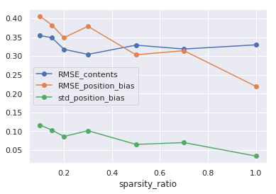
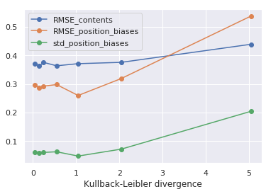
[[(Left)The relationship between RMSE and sparsity ratio (Right) The relationship between RMSE and Kullback Lierbler divergence.](Left) Yellow line shows the RMSE and sparsity$\_$ratio have negative correlation. (Right) Yellow shows the RMSE and KL divergence have positive correlation.

Figure 1. The RSME of position bias estimation against data-sparsity-ratio (left) and against Kullback–Leibler divergence between logging policy and uniform distribution (right).

The figure on the left in Fig.1 shows the Root Mean Square Error and standard deviation of estimated position bias (orange line) becomes lower as the sparsity ratio increases. The figure on the right in Fig.1 shows that these values become higher as Kullback-Leibler divergence becomes larger. Whereas the RMSE of the estimated probability to click contents (blue line) was nearly constant against the change of sparsity metrics.

5.2. Real-world dataset

As our next step, we aim to assess the accuracy of the existing embedding method in calculating $p(e|i)$, as well as the degree to which the No Direct Effect assumption is satisfied in the real-world dataset. To achieve this, we collected a logging dataset from an ”Annonymous e-commerce platform”. This platform features a carousel containing 15 advertisements, with 3 ads displayed simultaneously. When users click the right button, these ads are replaced with the next three banners. During a certain period, the logging policy was uniformly random, serving as a control group for an A/B test. However, during other periods, the logging policy was determined heuristically by marketers, leading to sparse pairs of (item, position).

5.2.1. How item embedding improves the position bias estimation in real-data

In terms of evaluating position bias, it is challenging to obtain the true position biases from a real-world dataset. Instead, we propose another method of assessing position bias. In the synthetic experiment shown in Fig.1, we demonstrated that the position bias estimated with a uniform and dense dataset had a lower RMSE than that estimated with a fixed logging policy. Therefore We treated the position biases with uniform random policy as the target value to be learned. We then dropped off item-position pairs to increase the sparsity of the dataset. As a result, we extracted a sparse sub-dataset that restricts an item to be assigned to a single position. We applied our proposed method to this sub-dataset and evaluated its performance in terms of how well we can predict the estimated position bias with a random policy from the sparse dataset with a fixed policy. Thus, we use RMSE as a performance metric when comparing the estimated position bias from the original dataset.

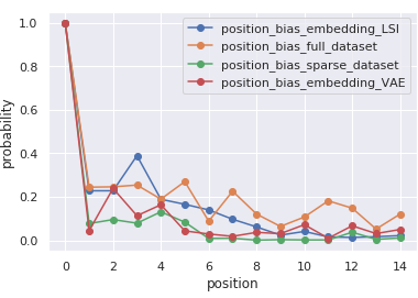
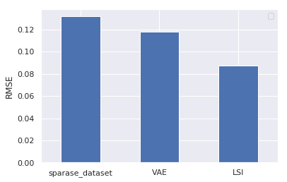
[(Left) The line plot of position bias at each position. (Right) The barplot of RMSE for each policy. VAE improved RMSE relatively by 10.3% and LSI improved RMSE relatively by 33.4%]

Figure 2. The comparison of position bias estimation among different behavior policies (left) and the RMSE (right).

(Left) The yellow line shows the position bias estimated from the logging dataset with uniform random policy. We regard this as the target line. The green line shows the position bias from the sparse sub-dataset with a fixed logging policy. The blue line shows the position bias from a fixed logging policy and Latent semantic indexing. The red line shows the position bias from a fixed logging policy and Variational Auto-Encoder. (Right) The Bar plot of RMSE.

Fig.2 shows the performance when we applied Latent Semantic Index and Variational Auto-Encoder to the real-world dataset. VAE improved RMSE relatively by 10.3% and LSI improved RMSE relatively by 33.4%. This result indicates our proposal method actually improved the estimation of position bias from the real logging dataset.

6. Conclusion and Future work.

We introduced the sparsity issue in the position bias estimation under the Position-based click model. Then with the synthetic data, we showed the metrics of sparsity such as sparsity ratio and Kullback-Leibler divergence are correlated to the RMSE of estimated position bias. To overcome the sparsity issue, we proposed the Regression EM algorithm with embedding. By utilizing the assignment probability $p(e|i)$, we sample various pairs of (embedding vector, position) and apply the Regression EM algorithm to estimate position bias with these samples. We prepared real traffic of clicking ads from the carousel of our e-commerce platform. Our empirical experiment shows that the Regression EM algorithm with VAE improves RMSE relatively by 10.3% and EM with LSI improves RMSE relatively by 33.4%.

References

- (1)
- Agarwal et al. (2019) Aman Agarwal, Ivan Zaitsev, Xuanhui Wang, Cheng Li, Marc Najork, and Thorsten Joachims. 2019. Estimating Position Bias without Intrusive Interventions. In Proceedings of the Twelfth ACM International Conference on Web Search and Data Mining (Melbourne VIC, Australia) (WSDM ’19). Association for Computing Machinery, New York, NY, USA, 474–482. https://doi.org/10.1145/3289600.3291017
- Aharon et al. (2019) Michal Aharon, Oren Somekh, Avi Shahar, Assaf Singer, Baruch Trayvas, Hadas Vogel, and Dobri Dobrev. 2019. Carousel ads optimization in yahoo gemini native. In Proceedings of the 25th ACM SIGKDD International Conference on Knowledge Discovery & Data Mining. 1993–2001.
- Ai et al. (2018) Qingyao Ai, Keping Bi, Cheng Luo, Jiafeng Guo, and W. Bruce Croft. 2018. Unbiased Learning to Rank with Unbiased Propensity Estimation. In The 41st International ACM SIGIR Conference on Research; Development in Information Retrieval (Ann Arbor, MI, USA) (SIGIR ’18). Association for Computing Machinery, New York, NY, USA, 385–394. https://doi.org/10.1145/3209978.3209986
- Arik and Pfister (2021) Sercan Arik and Tomas Pfister. 2021. TabNet: Attentive Interpretable Tabular Learning.
- Budhraj et al. (2022) Rahul Budhraj, Pooja Kherwa, Shreyans Sharma, and Sakshi Gill. 2022. Efficient Recommendation System Using Latent Semantic Analysis. 615–626. https://doi.org/10.1007/978-981-16-3071-2_50
- Cao et al. (2007) Zhe Cao, Tao Qin, Tie-Yan Liu, Ming-Feng Tsai, and Hang Li. 2007. Learning to rank: from pairwise approach to listwise approach. In Proceedings of the 24th international conference on Machine learning. 129–136.
- Chapelle and Chang (2011) Olivier Chapelle and Yi Chang. 2011. Yahoo! Learning to Rank Challenge Overview. In Proceedings of the Learning to Rank Challenge (Proceedings of Machine Learning Research, Vol. 14), Olivier Chapelle, Yi Chang, and Tie-Yan Liu (Eds.). PMLR, Haifa, Israel, 1–24. https://proceedings.mlr.press/v14/chapelle11a.html
- Chen et al. (2021) Yu Chen, Yingfeng Chen, Zhipeng Hu, Tianpei Yang, Changjie Fan, Yang Yu, and Jianye Hao. 2021. Learning Action-Transferable Policy with Action Embedding. arXiv:1909.02291 [cs.LG]
- Chuklin et al. (2015) Aleksandr Chuklin, Ilya Markov, and Maarten de Rijke. 2015. Click models for web search. Synthesis lectures on information concepts, retrieval, and services 7, 3 (2015), 1–115.
- Craswell et al. (2008) Nick Craswell, Onno Zoeter, Michael Taylor, and Bill Ramsey. 2008. An experimental comparison of click position-bias models. In Proceedings of the 2008 international conference on web search and data mining. 87–94.
- Devlin et al. (2018) Jacob Devlin, Ming-Wei Chang, Kenton Lee, and Kristina N. Toutanova. 2018. BERT: Pre-training of Deep Bidirectional Transformers for Language Understanding. https://arxiv.org/abs/1810.04805
- Hughes et al. (2019) Rachael A Hughes, Neil M Davies, George Davey Smith, and Kate Tilling. 2019. Selection bias when estimating average treatment effects using one-sample instrumental variable analysis. Epidemiology (Cambridge, Mass.) 30, 3 (2019), 350.
- Hurley and Rickard (2009) Niall Hurley and Scott Rickard. 2009. Comparing measures of sparsity. IEEE Transactions on Information Theory 55, 10 (2009), 4723–4741.
- Joachims et al. (2017) Thorsten Joachims, Laura Granka, Bing Pan, Helene Hembrooke, and Geri Gay. 2017. Accurately interpreting clickthrough data as implicit feedback. In Acm Sigir Forum, Vol. 51. Acm New York, NY, USA, 4–11.
- Keane and O’Brien (2006) Mark T Keane and Maeve O’Brien. 2006. Modeling result-list searching in the world wide web: The role of relevance topologies and trust bias. In Proceedings of the Annual Meeting of the Cognitive Science Society, Vol. 28.
- Kingma et al. (2019) Diederik P Kingma, Max Welling, et al. 2019. An introduction to variational autoencoders. Foundations and Trends® in Machine Learning 12, 4 (2019), 307–392.
- McCullagh (2008) Peter McCullagh. 2008. Sampling bias and logistic models. Journal of the Royal Statistical Society: Series B (Statistical Methodology) 70, 4 (2008), 643–677.
- Mikolov et al. (2013) Tomas Mikolov, Kai Chen, Greg Corrado, and Jeffrey Dean. 2013. Efficient estimation of word representations in vector space. arXiv preprint arXiv:1301.3781 (2013).
- Rendle et al. (2009) Steffen Rendle, Leandro Balby Marinho, Alexandros Nanopoulos, and Lars Schmidt-Thieme. 2009. Learning optimal ranking with tensor factorization for tag recommendation. In Proceedings of the 15th ACM SIGKDD international conference on Knowledge discovery and data mining. 727–736.
- Richardson et al. (2007) Matthew Richardson, Ewa Dominowska, and Robert Ragno. 2007. Predicting clicks: estimating the click-through rate for new ads. In Proceedings of the 16th international conference on World Wide Web. 521–530.
- Rosario (2000) Barbara Rosario. 2000. Latent semantic indexing: An overview. Techn. rep. INFOSYS 240 (2000), 1–16.
- Saito and Joachims (2022) Yuta Saito and Thorsten Joachims. 2022. Off-Policy Evaluation for Large Action Spaces via Embeddings. arXiv preprint arXiv:2202.06317 (2022).
- Wang et al. (2016) Xuanhui Wang, Michael Bendersky, Donald Metzler, and Marc Najork. 2016. Learning to Rank with Selection Bias in Personal Search (SIGIR ’16). Association for Computing Machinery, New York, NY, USA, 115–124. https://doi.org/10.1145/2911451.2911537
- Wang et al. (2018) Xuanhui Wang, Nadav Golbandi, Michael Bendersky, Donald Metzler, and Marc Najork. 2018. Position bias estimation for unbiased learning to rank in personal search. In Proceedings of the Eleventh ACM International Conference on Web Search and Data Mining. 610–618.
- Yuan et al. (2017) Fajie Yuan, Guibing Guo, Joemon M Jose, Long Chen, Haitao Yu, and Weinan Zhang. 2017. Boostfm: Boosted factorization machines for top-n feature-based recommendation. In Proceedings of the 22nd International Conference on Intelligent User Interfaces. 45–54.
- Yue et al. (2010) Yisong Yue, Rajan Patel, and Hein Roehrig. 2010. Beyond position bias: Examining result attractiveness as a source of presentation bias in clickthrough data. In Proceedings of the 19th international conference on World wide web. 1011–1018.
- Zhao et al. (2020) He Zhao, Piyush Rai, Lan Du, Wray Buntine, Dinh Phung, and Mingyuan Zhou. 2020. Variational autoencoders for sparse and overdispersed discrete data. In International Conference on Artificial Intelligence and Statistics. PMLR, 1684–1694.