Towards Optimal Serverless Function Scaling
in Edge Computing Network

Abstract

Serverless computing has emerged as a new execution model which gained a lot of attention in cloud computing thanks to the latest advances in containerization technologies. Recently, serverless has been adopted at the edge, where it can help overcome heterogeneity issues, constrained nature and dynamicity of edge devices. Due to the distributed nature of edge devices, however, the scaling of serverless functions presents a major challenge. We address this challenge by studying the optimality of serverless function scaling. To this end, we propose Semi-Markov Decision Process-based (SMDP) theoretical model, which yields optimal solutions by solving the serverless function scaling problem as a decision making problem. We compare the SMDP solution with practical, monitoring-based heuristics. We show that SMDP can be effectively used in edge computing networks, and in combination with monitoring-based approaches also in real-world implementations.

I Introduction

In the cloud, Function-as-a-Service (FaaS) computing model provides for fast autoscaling, by removing decision-making on scaling thresholds; reduces starting times, by using containerization as underlying technology; and provides easy capacity planning, by only charging when resources are used; albeit at costs of losing control on the deployment environment by the developers. In edge computing, however, such scaling of services is challenged by the distributed nature and heterogeneity of devices in edge network nodes as well as the resulting performance variability. To overcome these limitations, the serverless execution model with scaling features is envisioned as a prime mechanism in edge computing networks.

Studies adapting and further developing the well-known cloud computing scaling mechanisms are few and far between in the edge context. Since function provider mechanism can scale based on different parameters, such as by the number of requests per second, CPU or memory resource utilization among others, determining which mechanism is more appropriate in the edge is an open challenge. Considering that edge nodes are distributed, constrained computing and networked units, heterogeneous and volatile, optimal scaling methods are non-trivial on these type of dynamic networked systems.

In this paper, we address the optimality of serverless scaling in edge computing network. We propose Semi-Markov Decision Process-based (SMDP) model for the scaling problem of serverless functions as a decision making problem, with actions of scaling the functions up or down, the reward depending on processing and queueing costs. The SMDP model maximizes the long-term expected reward of the system, considering the system gains, costs of queueing and resource utilization. SMDP enables us to obtain the optimal solution where it can be also decided on the next action at each system state. From the practical perspective, our model does not need to know which function is running in which node, thus making the telemetry in edge network rather practical. The theoretical results are compared with practical, monitoring-based algorithms. We show that this novel application of SMDP can be effectively used for function scaling, and in combination with monitoring-based approaches also in real-world edge network implementations, e.g. with OpenFaaS.

The rest of the paper is organized as follows. Section II describes the related work. Section III introduces the SMDP model. Section IV evaluates the performance. Section V concludes the paper.

II Related Work

Function scaling, - a process of increasing or decreasing a number of function replicas, - is solved in a centralized manner both commercially, such as in Amazon AWS Lambda or Google Cloud Functions, and in open source serverless platforms, such as OpenFaaS or Apache OpenWhisk. While previous work adopts these platforms to the edge context, including [1], [2], there is lack of specific scaling mechanisms designed to work for this type of systems. Related theoretical works studying aspects such as job scheduling [3], resource provisioning [4] and placement of resources [5] have been proposed in this context. These solutions, however, assume periodic collection of telemetry data to provide optimal solutions, such as resources state and users’ demand of functions. This requires linear programing models, which are known to be computationally demanding. From the practical perspective, computationally complex optimization models cannot adequately consider software limitations in terms of decision times, complexity of the related telemetry, etc. In addition, joint solutions for functions of scaling, edge node allocation and scheduling are complex to implement, as they use multiple and diverse multiple tools when orchestrating services.

To the best of our knowledge, this paper is the first to study optimal scaling serverless functions problem theoretically by using SMDP modeling. We found inspiration to using SMDP model from a few related works, that used this method in different context. In [6] and [7], SMDP-based resource allocation schemes were used in vehicular networks for quality of experience. The paper considers the service requests from vehicles and decides whether to process it locally or to transfer to other nodes, considering the reward and constraints of each possible action. The reward consists of the income and costs of power consumption and processing time. In [8], SMDP was used for coordinated virtual machine (VM) allocation for a cloud-fog computing system, considering the balance between the high cost of communication to the cloud and and the limited fog capacity.

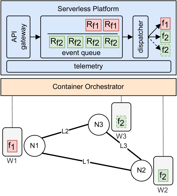
Figure 1: Serverless system at the edge

III SMDP-based Scaling model

Our system model is illustrated in Fig. 1. It consists of a set of edge computing nodes (i.e., W1, W2 and W3), serverless platform and container orchestrator (e.g., Kubernetes), all generally located in different parts of the network. The serverless platform (e.g., OpenFaaS) is instantiated on the cluster with access to all the resources and bundles the API gateway, event queue, dispatcher and telemetry components. The API gateway handles HTTP requests from the users requesting functions and creates events. The event queues allocates different queues per type of function requests where they wait to be served. The dispatcher is responsible for scaling decisions to be made per type of function based on the number of requests and on the resource utilization. For instance, in openFaaS, we monitor the arrival rate (or load) and whenever it exceeds a threshold for a specific function, new replicas are created; whenever the queue is empty it removes the replicas. The information about arrival event and the queue information is collected by the telemetry component through an API exposed by the container orchestrator. The scaling decisions are sent to the container orchestrator which actually creates or removes replicas of functions from the nodes, depending on whether the system is scaling up or down. The container orchestrator is responsible for placing the function replicas on edge nodes.

III-A Problem Formulation

We assume a single master deployment and a set of edge nodes denoted as $\mathcal{E}=\{E_{1},..,E_{n},...,E_{N}\}$, where $E_{n}$ represents the $n^{\text{th}}$ edge node. Each edge node has a certain amount of capacity which we refer to as a number of CPU units $C_{n}$. Every specific function requires a certain amount of resources. Thus, we categorize all function requests into $K$ classes based on their resource needs. A function request of class $k$, where $1\leq k\leq K$, is denoted as $f_{k}$, and requires $b_{k}$ CPU units, whereby $b_{k}\leq max_{\forall n:n\in[1,N]}\{C_{n}\}$, i.e., for any function $f_{k}$, there exist at least one edge node $E_{n}$ with enough capacity $C_{n}$ to satisfy the request. We model the arrival and service processes of function requests of class $k$ as a Poisson process with rates $\lambda_{k}$, and $\mu_{k}$, respectively. We assume that all function requests are queued in a buffer with infinite capacity. The proposed SMDP model is described by the components {$S$, $A(s)$, $p(s^{\prime}|s,a)$, $r(s|a)$}, where $S$ is the state space, $A(s)$ is the set of feasible actions at the state $s\in S$, $p(s^{\prime}|s,a)$ is the transition probability from the state $s$ to the state $s^{\prime}$ when an action $a$ is chosen, and $r(s|a)$ is the reward of the system at the state $s$ when choosing the action $a$.

III-B System States

The system state $s$ represents the number of replicas of each function $k$ in all nodes $E_{n}$, the number of function requests of each service class $k$ in the queue, and the a set of events that can happen in the system:

$$\begin{split}S=\{s|s=&(\Delta,Q,e)\},\end{split}$$ (1)

where a set $\Delta=\delta_{1},...,\delta_{k},...,\delta_{K}$ indicates a number of functions, where the variable $\delta_{k}$ denotes the number of functions of class $k$ replicated in all nodes. $Q=\{Q_{1},...,Q_{K}\}$ denotes the function request queue length vector. The variable $e$ describes an event that occurs in the system, such as $e=\{Ar,D\}$, where a set $Ar=\{Ar_{1},...,Ar_{k},...,Ar_{K}\}$ contains the arrival events of any function request of the class $k$, a set $D=\{D_{1},...,D_{k},...,D_{K}\}$, and a subset $D_{k}=\{D_{1}^{n},...,D_{k}^{n},...,D_{K}^{n}\}$ collects the set of departure events of a function of class $k$, and $D_{k}^{n}$ defines the departure event of a function of class $k$ from node $E_{n}$.

The resource allocation has the capacity constraints, i.e.,

$$\forall n\in[1,N]:\sum_{k=1}^{K}b_{k}\delta_{k}(n)\leq C_{n},$$ (2)

The dispatcher (scaler) has three possibilities of actions $a$ to take for every new event (arrival or departure): to scale up, to scale down or to do nothing. The action space $A(s)$ is described as follows:

$$A(s)=\begin{cases}\{0,1\},\;&e\in Ar\\ \{-1,0\},\;&e\in D\\ \end{cases}$$ (3)

where $a(s)=1,\forall k\in\{1,...,K\}$ when a function of class $k$ is replicated, $a(s)=-1,\forall k\in\{1,...,K\}$ when a function of class $k$ is removed from the system, $a(s)=0$ denotes the action of queuing a function request of any class $k$, without replication in the case of a function arrival, and the queue update without removing function replica in the case of function request departure.

III-C Transition Probabilities

At time slot $t_{i+1}$, the $f_{k}$ request queue length can be expressed as:

$$\begin{split}Q_{k}(t_{i+1})=Q_{k}(t_{i})+\mathds{1}(a(s)=0||e=A_{k})\\ -\mathds{1}(a(s)=0||e\in D_{k})\end{split}$$ (4)

where $Q_{k}(t_{i})$ describes the previous $f_{k}$ request queue length when the $i^{\text{th}}$ event occurs, $\mathds{1}(.)$ describes the identity operator. The number of functions of class $k$ replicated in all edge nodes can be expressed as follows:

$$\begin{split}\delta_{k}(t_{i+1})=\delta_{k}(t_{i})+\mathds{1}(a(s)=1||e=A_{k})\\ -\mathds{1}(a(s)=-1||e\in D_{k}^{n})\end{split}$$ (5)

We assume that the time period between two continuous decision epochs follows an exponential distribution and denoted as $\tau(s,a)$, given the current state $s$ and action $a$. Thus the mean rate of events for a specific state $s$ and action $a$ denoted as $\gamma(s,a)$, is the sum of the rates of all events in the system, which is expressed as follows:

$$\begin{split}&\forall n\in\{1,...,N\},\forall k\in\{1,...,K\}:\\ &\text{ }\tau(s,a)=\gamma(s,a)^{-1}=\\ &\begin{cases}\Lambda+\Theta+\mu_{k},\;&e=Ar_{k},a=1,\\ \Lambda+\Theta,&e=Ar_{k},a=0,\\ \Lambda+\Theta-\mu_{k},&e=D_{k}^{n},a=-1,\\ \Lambda+\Theta,&e=D_{k}^{n},a=0\end{cases}\end{split}$$ (6)

where $\Lambda=\sum_{k=1}^{K}\lambda_{k}$ is the total arrival rate of function requests of all $K$ function classes. When a function request arrives and the dispatcher decides not to replicate, or a function request leaves an edge node and the dispatcher decides not to remove a function from the nodes, the total number of existing functions in the system is $\sum_{k=1}^{K}\delta_{k}$, so the departure rate of a function in the edge computing is $\Theta=\sum_{k=1}^{K}\delta_{k}\mu_{k}$. When a function request of class $k$ is replicated, one function of class $k$ is added to the system, thus the departure rate becomes $\Theta+\mu_{k}$. When a departure of a function of class $k$ occurs and the dispatcher removes a replica from the system, the departure rate becomes $\Theta-\mu_{k}$.

The transition probability in our markov decision model from state $s$ to state $s^{\prime}$ when an action $a$ is selected is denotes as $p(s^{\prime}|s,a)$, which can be determined under different events:

i) State $s=(\Delta,Q,Ar_{k})$, and $a=0$

This state describes the system in terms of number of functions allocated in all nodes, the number of function requests in the queue, and the next event, which is in this case a function request arrival of class $k$. The function arrival event can have two types of actions replicate or not to replicate. The following equation shows the transition probability when the function is queued without replication, where the number of functions allocated in all nodes remains the same, and function request queue length $\widehat{Q}$ is updated using eq. (4), and possible events can occur in the future.

$$\begin{split}&p(s^{\prime}|s,a)=\begin{cases}\frac{\lambda_{k^{\prime}}}{\tau(s,a)}&s^{\prime}=(\Delta,\widehat{Q},Ar_{k^{\prime}})\\ \frac{\delta_{k^{\prime}}\mu_{k^{\prime}}}{\tau(s,a)}&s^{\prime}=(\Delta,\widehat{Q},D_{k^{\prime}}^{n})\end{cases}\end{split}$$ (7)

ii) State $s=(\Delta,Q,Ar_{k})$, $a=1$

This state is defined similar to the previous state, considering creating a new replica.

$$\begin{split}&p(s^{\prime}|s,a)=\begin{cases}\frac{\lambda_{k^{\prime}}}{\tau(s,a)}&s^{\prime}=(\widehat{\Delta},Q,Ar_{k^{\prime}}),\\ \frac{\delta_{k^{\prime}}\mu_{k^{\prime}}}{\tau(s,a)}&k^{\prime}\neq k,\\ &s^{\prime}=(\widehat{\Delta},Q,D_{k^{\prime}}^{n})\\ \frac{(\delta_{k}+1)\mu_{k}}{\tau(s,a)}&s^{\prime}=(\widehat{\Delta},Q,D_{k}^{n})\\ \end{cases}\end{split}$$ (8)

where $\widehat{\Delta}=\{\delta_{1},...,\delta_{k}+1,...,\delta_{K}\}$.

iii) State $s=(\Delta,Q,D_{k}^{n})$, and $a=0$

The next event in this state is a function request departure of class $k$ from edge node $E_{n}$. The function departure event can have two types of actions remove or not remove a function replica. The following equation shows the transition probability when the function leaves the system without removing a function replica, where the number of functions allocated in all edge nodes remains the same, and function request queue length $\widehat{Q}$ is updated using eq. (4), and possible events can occur in the future.

$$\begin{split}&p(s^{\prime}|s,a)=\begin{cases}\frac{\lambda_{k^{\prime}}}{\tau(s,a)}&s^{\prime}=(\Delta,\widehat{Q},Ar_{k^{\prime}})\\ \frac{\delta_{k^{\prime}}\mu_{k^{\prime}}}{\tau(s,a)}&s^{\prime}=(\Delta,\widehat{Q},D_{k^{\prime}}^{n})\end{cases}\end{split}$$ (9)

iv) State $s=(\Delta^{\prime},Q,D_{k}^{n})$, $a=-1$

This state is defined similar to the previous state, considering removing a replica.

$$\begin{split}&p(s^{\prime}|s,a)=\begin{cases}\frac{\lambda_{k^{\prime}}}{\tau(s,a)}&s^{\prime}=(\widehat{\Delta},Q,Ar_{k^{\prime}}),\\ \frac{\delta_{k^{\prime}}\mu_{k^{\prime}}}{\tau(s,a)}&k^{\prime}\neq k\\ &s^{\prime}=(\widehat{\Delta},Q,D_{k^{\prime}}^{n})\\ \frac{(\delta_{k}-1)\mu_{k}}{\tau(s,a)}&s^{\prime}=(\widehat{\Delta},Q,D_{k}^{n})\\ \end{cases}\end{split}$$ (10)

where $\widehat{\Delta}=\{\delta_{1},...,\delta_{k}-1,...,\delta_{K}\}$.

III-D Rewards

Given the system state $s$ and the corresponding action $a$, the system reward of the function provider is denoted by

$$r(s,a)=w(s,a)-g(s,a)$$ (11)

where $w(s,a)$ is the net lump sum incomes of the system at the state $s$ when action $a$ is taken and an event $e$ occurs, and $g(s,a)$ is the expected system costs.

$$\begin{split}w(s,a)=\begin{cases}w_{k}&e=Ar_{k},a\in\{0,1\}\\ 0&e=D_{k}^{n},a=\{0,-1\}\\ \end{cases}\end{split}$$ (12)

where the variable $w_{k}$ denotes the reward of the system for accepting of a function request of class $k$. The expected system cost $g(s,a)$ is defined as:

$$g(s,a)=c(s,a)\cdot\tau(s,a)$$ (13)

where $\tau(s,a)$ is the expected service time defined by eq. (6) from the state $s$ to the next state in case that action $a$ is chosen and $c(s,a)$ is the service holding cost rate when the system is in state $s$ in case that action a is selected, which depends on the queuing. Furthermore, $c(s,a)$ can be described by the number of occupied resources in the system, the queue length using Little’s Law, as follows:

$$\begin{split}&c(s,a)=\underbrace{\sum_{k=1}^{K}c\cdot b_{k}\cdot\delta_{k}}_{\text{Processing}}+\underbrace{\sum_{k=1}^{K}\frac{Q_{k}}{\lambda_{k}}}_{\text{Queuing}}\end{split}$$ (14)

where $c$ represents the utilization cost of a resource unit. In order to only optimize the delay, the processing cost can be ignored by setting $c$ to $0$.

III-E SMDP-based Scaling Model

We develop an SMDP-based Scaling Model (SM) to study the performance of a serverless platform considering the queuing and processing delay of function requests. We aim at taking the optimal decisions at every decision event (arrival of new function request, and departure of a function request) where our goal is to maximize the long-term expected system rewards. The expected discounted reward is given based on the model in [9] as follows:

$$\begin{split}r(s,a)=&w(s,a)-c(s,a)\cdot E_{s}^{a}\{\int_{0}^{\tau}e^{-\alpha t}dt\}\\ =&w(s,a)-c(s,a)\cdot E_{s}^{a}\{\frac{1-e^{-\alpha\tau}}{\alpha}\}\\ =&w(s,a)-\frac{c(s,a)}{\alpha+\tau(s,a)}\\ \end{split}$$ (15)

where $\alpha$ is a continuous-time discount factor.

Using the defined transition probabilities eq. (7), (8), (9), (10), we can obtain the maximum long-term discounted reward using a discounted reward model defined in [9] as

$$\nu(s)=\max_{a\in A(s)}\left\{r(s,a)+\lambda\sum_{s^{\prime}\in S}p(s^{\prime}|s,a)\nu(s^{\prime})\right\}$$ (16)

where $\lambda=\tau(s,a)/(\alpha+\tau(s,a))$. In the SMDP model, the value of $\nu(s)$ in a strategy $\psi$ is computed based on the value $\nu(s^{\prime})$ obtained in the strategy $\psi-1$, and as an initial value, the discounted reward can be set to zero for all states to initialize the computation, which converges afterwards towards the optimal solution.

To simplify the computation of the reward, let $\rho$ be a finite constant, where $\rho=\sum_{i=1}^{K}\lambda_{i}+\sum_{n=1}^{N}\sum_{k=1}^{K}C_{n}\mu_{k}<\infty$. We define $\overline{p}(s^{\prime}|s,a)$, $\overline{\nu}(s)$, and $\overline{r}(s,a)$ as the uniformed transition probability, long-term reward, and reward function, respectively, and given by:

$$\overline{r}(s,a)=r(s,a)\frac{\tau(s,a)+\alpha}{\rho+\alpha},\overline{\lambda}=\frac{\rho}{\rho+\alpha}$$ (17)

$$\begin{split}\overline{p}(s^{\prime}|s,a)=\begin{cases}1-\frac{[1-p(s^{\prime}|s,a)]\tau(s,a)}{\rho}&s^{\prime}=s\\ \frac{p(s^{\prime}|s,a)\tau(s,a)}{\rho}&s^{\prime}\neq s\\ \end{cases}\end{split}$$ (18)

After uniformization, the optimal reward is given by:

$$\overline{\nu}(s)=\max_{a\in A(s)}\left\{\overline{r}(s,a)+\overline{\lambda}\sum_{s^{\prime}\in S}\overline{p}(s^{\prime}|s,a)\overline{\nu}(s^{\prime})\right\}$$ (19)

In order to solve our SMDP-SM, we use the iterative algorithm described as follows:

Algorithm 1 Iterative SMDP-SM Algorithm

1:Step 1 (Initialization): $\overline{\nu}^{0}(s)=0$, for all $s\in S$. Set the value of $\epsilon>0$, and iteration $t=0$.

2:Step 2: Using eq. 19, compute the discounted reward for each state $s$:

$$\overline{\nu}^{t+1}(s)=\max_{a\in A(s)}\left\{\overline{r}(s,a)+\overline{\lambda}\sum_{s^{\prime}\in S}\overline{p}(s^{\prime}|s,a)\overline{\nu}^{t}(s^{\prime})\right\}$$

3:Step 3:

4:if $\|\overline{\nu}^{t+1}-\overline{\nu}^{t}\|>\epsilon$  then $t\longleftarrow t+1$, go to Step 2

5:else  go to Step 4

6:end if

7:Step 4: Compute the optimal scaling policy for all $s\in S$

$$d_{\epsilon}^{*}(s)\in\text{arg}\max_{a\in A(s)}\left\{\overline{r}(s,a)+\overline{\lambda}\sum_{s^{\prime}\in S}\overline{p}(s^{\prime}|s,a)\overline{\nu}^{t+1}(s^{\prime})\right\}$$

After obtaining the optimal policy from Algorithm 1, the steady states probabilities are computed as, i.e.,

$$\begin{split}\pi(P-J)=0,\sum_{s\in S}\pi(s)=1\end{split}$$ (20)

where $\pi(s)$ represents the steady state probability at state $s$, $P$ is the transition probabilities matrix, considering the optimal policy $d_{\epsilon}^{*}$, and $J$ denotes the all-ones matrix.

The Algorithm 1 is executed offline after defining the network topology in order to find the optimal scaling policies for every possible system state. Afterward the optimal policies are used online as a look-up table to make scaling decision with a time complexity of $O(1)$.

III-F Complexity Analysis

Consider the case with $N$ nodes, $K$ functions, the time complexity of Algorithm 1, which is based on Policy Iteration algorithm depends on the number of states $|S|$, number of actions $|A|$ and the discount factor $\gamma$. Scherrer [10] has proven that Policy Iteration terminates after at most $O\left(\frac{|S|\cdot|A|}{1-\gamma}\log\left(\frac{1}{1-\gamma}\right)\right)$. The number of states can be represented in terms of the network configuration parameters using eq. (1), as combination of possible number of replicas of each function, the state of the queues, and the number of possible next events (arrival or departure). Assuming that the system can have a maximum number of replicas per function denoted as $M$, and a maximum queue length $Q_{m}$, $|S|=M^{K}\cdot Q_{m}^{K}\cdot(K+K\cdot N)$. The number of actions in our proposal is equal to 3. Thus the time complexity of Algorithm.1 is given by:

$$O\left(\frac{M^{K}\cdot Q_{m}^{K}\cdot K\cdot(N+1)}{1-\gamma}\log\left(\frac{1}{1-\gamma}\right)\right)$$ (21)

Space complexity of the algorithm is mainly driven by the storage of the states information generated at the initialization phase and given by:

$$O\left(M^{K}\cdot Q_{m}^{K}\cdot K\cdot(N+1)\right)$$ (22)

IV Numerical results

We now evaluate the performance of the SMDP scaling methods, by comparing it to the monitoring-based heuristics, and for the sake of verification, by comparing it to a random-fit model. The monitoring-based methods are relevant to evaluation, since they are used today, e.g., in OpenFaaS. In OpenFaaS, for instance, the scaling decisions consider arrival rates by default. In practice, the theoretical time complexity is in fact $O(1)$. As shown in Fig. 1, the serverless platform includes the monitoring-based scaling, where the telemetry collects information about the load. Whenever the load exceeds a certain threshold, the monitoring algorithm triggers the system to create new replicas, and whenever the queue becomes empty, the algorithm decides to remove replicas, otherwise it keeps the same system state. The monitoring-based algorithm is thus described as follows:

Algorithm 2 Monitoring-based scaling algorithm

1:Input: event, queue, capacity, load, threshold

2:if event is an arrival  then

3:     if capacity is available then

4:         if load > threshold then return 1

5:         else return 0

6:         end if

7:     else return 0

8:     end if

9:end if

10:if event is a departure  then

11:     if the queue is empty  then return -1

12:     else  return 0

13:     end if

14:end if

For comparison purposes, we also show random-fit scaling (theoretical time complexity $O(1)$), that decides randomly either to scale or not, if there are available resources. The algorithm follows the same structure as in the monitoring based approach with the only difference that in line 4, instead of checking the threshold, we just return a random node.

We evaluate the performance of the three scaling methods using: i) SMDP model, ii) monitoring-based (MNT) and iii) random-fit (RF). Since scaling decisions do not determine function allocations, we assume two simple allocation approaches: First-Fit allocation (FFa) and Random-Fit allocation (RFa). In FFa, functions are allocated in the closest available node, considering a network with a single master and multiple workers. In RFa, functions are allocated randomly in any available node with enough available resources. All three scaling methods are then evaluated considering both FFa and RFa. We evaluate two networks, a small one with 3 edge nodes and a big one with 10 nodes. We use the small one for comparing all methods, with threshold numbers $0.1$ and $0.05$. And, we use the large network to compare the performance of only heuristics, with threshold numbers $0.01$, $0.005$ and $0.001$. For generating the results, we use an event based simulator running up to 1 million events with severals seeds to validate our results. The rest of the parameters are shown in Table I.

Table I: Simulation Parameters.

Parameters	$N$	$K$	$b_{k}$	$C_{n}$	$c$	$w_{k}$	$\lambda_{k}$	$\mu_{k}$
Small network	3	5	$k$	16	1	1	2-11	1-11
Large network	10	10	$k$	100	1	1	4-12	10-$10^{2}$

Fig. 2 shows the average service delay of all functions for arrival rates of requests for each scaling algorithm in the small network. The results shows that SMDP overperforms all other approaches for any value of arrival rate. The delay obtained by monitoring based approach decreases with the decrease of the threshold value and outperforms the random approach until a certain value of arrival rate $\lambda$, after which the delay starts to increase exponentially, at $\lambda=9.6$ in Figure 2. This behavior is created by the accumulation of function requests in the queue when the load becomes constantly lower than the threshold, resulting a cumulative queueing delay. The delay results using First-Fit allocation is slightly better than the results obtained with a Random-Fit allocation, which can be explained by the fact that the average delay is mostly affected by the queueing and less by the transmission delay.

Figure 3 shows the average number of replicas of all functions with different arrival rates of function requests for each scaling and allocation algorithm. The results shows that the chosen algorithm does not affect the number of replicas of each function, where both curves coincide. The highest average number of replicas is obtained with SMDP, which explains its performance in terms of delay. As expected, the lowest number of replicas is obtained by the RF approach.

Figure 4 illustrates the average service delay of all functions with different arrival rates of function requests. The monitoring-based approach with a very low threshold value $0.001$ outperforms the random approach, where its performance improves while decreasing the threshold value. A similar behavior is found in the small network for high threshold values, where monitoring-based approach outperforms the random approach until a certain value of arrival rate $\lambda$, after which the delay starts to increase exponentially. Finally, we illustrate in Figure 5 the average number of replicas for the large network. Similar to the small network, the allocation algorithm choice does not affect the number of replicas and Monitoring-based approach with the lowest threshold value creates larger number of replicas.

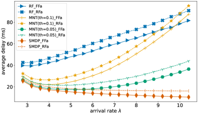
Figure 2: Average service delay per scaling model (small network).

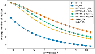
Figure 3: Average number of replicas per scaling model (small network).

V Conclusion

In this paper, we addressed the optimality of serverless scaling in edge computing network and proposed to use Semi-Markov Decision Process-based (SMDP) model for the scaling problem of serverless functions as a decision making problem, with actions of scaling the functions up or down. The theoretical results were compared with practical, monitoring-based algorithms based on current approaches.The results confirmed that SMDP gave best results in terms of queuing delay, and outperformed monitoring-based approaches. The monitoring-based approach however achieved performance comparable to the optimal SMDP solution in terms of delay when the scaling activation threshold was set to comparably lower values.In our future work, we will study the joint scaling and resource allocation problem considering various system parameters. SMDP can be used to analyse the optimal policy for a specific setting. Monitoring based is what is used in real implementations now, which can be more optimized using smarter algorithms such as SMDP. The issue of SMDP is its exponential expansion, so a heuristic based on SMDP can be a very good approach for future.

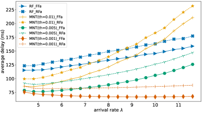
Figure 4: Average service delay per scaling model (large network).

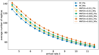
Figure 5: Average number of replicas per scaling model (large network).

References

- [1] F. Carpio, M. Michalke, and A. Jukan, “Benchfaas: Benchmarking serverless functions in an edge computing network testbed,” IEEE Network, pp. 1–8, 2022.
- [2] L. Baresi and D. F. Mendonça, “Towards a serverless platform for edge computing,” in 2019 IEEE International Conference on Fog Computing (ICFC). IEEE, 2019, pp. 1–10.
- [3] H. Tan, Z. Han, X.-Y. Li, and F. C. Lau, “Online job dispatching and scheduling in edge-clouds,” in IEEE INFOCOM 2017-IEEE Conference on Computer Communications. IEEE, 2017, pp. 1–9.
- [4] O. Ascigil, A. Tasiopoulos, T. K. Phan, V. Sourlas, I. Psaras, and G. Pavlou, “Resource provisioning and allocation in function-as-a-service edge-clouds,” IEEE Transactions on Services Computing, 2021.
- [5] M. Bensalem, J. Dizdarević, and A. Jukan, “Modeling of deep neural network (dnn) placement and inference in edge computing,” in 2020 IEEE International Conference on Communications Workshops (ICC Workshops), 2020, pp. 1–6.
- [6] H. Liang, X. Zhang, X. Hong, Z. Zhang, M. Li, G. Hu, and F. Hou, “Reinforcement learning enabled dynamic resource allocation in the internet of vehicles,” IEEE Transactions on Industrial Informatics, vol. 17, no. 7, pp. 4957–4967, 2020.
- [7] K. Zheng, H. Meng, P. Chatzimisios, L. Lei, and X. Shen, “An smdp-based resource allocation in vehicular cloud computing systems,” IEEE Transactions on Industrial Electronics, vol. 62, no. 12, 2015.
- [8] Q. Li, L. Zhao, J. Gao, H. Liang, L. Zhao, and X. Tang, “Smdp-based coordinated virtual machine allocations in cloud-fog computing systems,” IEEE Internet of Things Journal, vol. 5, no. 3, 2018.
- [9] M. L. Puterman, Markov decision processes: discrete stochastic dynamic programming. John Wiley & Sons, 2014.
- [10] B. Scherrer, “Improved and generalized upper bounds on the complexity of policy iteration,” Advances in Neural Information Processing Systems, vol. 26, 2013.