The Context Model: A Graph Database Model

Abstract

In the relational model a relation over a set of attributes is defined to be a (finite) subset of the Cartesian product of the attribute domains, separately from the functional dependencies that the relation must satisfy in order to be consistent. In this paper we propose to include the functional dependencies in the definition of a relation by introducing a data model based on a graph in which the nodes are attributes, or Cartesian products of attributes, and the edges are the functional dependencies.

Such a graph actually represents the datasets of an application and their relationships, so we call it an application context or simply context. We define a database over a context $\mathcal{C}$ to be a function $\delta$ that associates each node $X$ of $\mathcal{C}$ with a finite set of values $\delta(X)$ from the domain of $X$ and each edge $e:X\to Y$ with a total function $\delta(e):\delta(X)\to\delta(Y)$. We combine the nodes and edges of a context using a functional algebra in order to define queries; and the set of all well-formed expressions of this algebra is the query language of the context. A relation over attributes $A_{1},\ldots,A_{n}$ is then defined as a query whose paths form a tree with leaves $A_{1},\ldots,A_{n}$ and whose root is the key.

The main contributions of this paper are as follows: (a) we introduce a novel graph database model, called the context model, (b) we show that a consistent relational database can be embedded in the context model as a view over the context induced by its functional dependencies, (c) we define analytic queries in the query language of a context in a seamless manner - in contrast to the relational model where analytic queries are defined outside the relational algebra, and (d) we show that the context model can be used as a user-friendly interface to a relational database for data analysis purposes.

1 Introduction

The basic idea underlying this work is that the datasets of an application and their relationships can be seen as a labeled directed graph in which the nodes are the datasets and each edge is a function from its source node to its target node. We call such a graph an application context (or simply context).

The concept of context was first introduced in DBLP:conf/fqas/Spyratos06  SpyratosS18 as a means for defining analytic queries, in the abstract, and then translating them as queries to underlying query evaluation mechanisms such as SQL, MapReduce or SPARQL. In this paper we build upon these earlier works to propose a full fledged data model.

Let us borrow an example from SpyratosS18 to explain what a context is. Suppose $Inv$ is the set of all delivery invoices, say over a year, in a distribution center (e.g. Walmart) which delivers products of various types in a number of branches. A delivery invoice has an identifier (e.g. an integer) and shows the date of delivery, the branch in which the delivery took place, the type of product delivered (e.g. $CocaLight$) and the quantity (i.e. the number of units delivered of that type of product). There is a separate invoice for each type of product delivered, and the data on all invoices during the year is stored in a database for analysis and planning purposes.

Conceptually, the information provided by each invoice would most likely be represented as a tuple of a relation $R$ with the following attributes: Invoice number ($Inv$), $Date$, $Branch$, Product ($Prod$) and Quantity ($Qty$) with Invoice number as the key. Now, as $Inv$ is the key, we have the following key dependencies:

$d:Inv\to Date,~{}~{}b:Inv\to Branch,~{}~{}p:Inv\to Prod,~{}~{}q:Inv\to Qty$

These dependencies form a graph $\mathcal{C}$ as shown in Figure 1(a) (actually a tree in this case).

Think now of a mapping $\delta$ that associates the nodes and edges of $\mathcal{C}$ with projections over $R$ as follows:

Nodes: $\delta(Inv)=\pi_{Inv}(R)$,   $\delta(Date)=\pi_{Date}(R)$,   $\delta(Branch)=\pi_{Branch}(R)$,   $\delta(Prod)=\pi_{Prod}(R)$,   $\delta(Qty)=\pi_{Qty}(R)$

Edges: $\delta(d)=\pi_{Inv,Date}(R)$,   $\delta(b)=\pi_{Inv,Branch}(R)$,   $\delta(p)=\pi_{Inv,Prod}(R)$,   $\delta(q)=\pi_{Inv,Qty}(R)$

Clearly, if $R$ is consistent then each of the assignments $\delta(d)$, $\delta(b)$, $\delta(p)$ and $\delta(q)$ is a total function. Moreover all these functions have the same domain of definition, namely the projection $\pi_{Inv}(R)$ of $R$ over its key $Inv$.

Following this view, given an invoice number $i$ in $\delta(Inv)$, the function $\delta(d)$ returns a date $\delta(d)(i)$, the function $\delta(b)$ returns a branch $\delta(b)(i)$, the function $\delta(p)$ returns a product type $\delta(p)(i)$ and the function $\delta(q)$ returns a quantity $\delta(q)(i)$ (i.e. the number of units of product type $\delta(p)(i)$). Moreover by ‘pairing’ these four functions we recover the relation $R$ that is:

$R=\delta(d)\wedge\delta(b)\wedge\delta(p)\wedge\delta(q)$, where ‘$\wedge$’ denotes the operation of pairing

In this paper, given two functions $f:X\to Y$ and $g:X\to Z$ with a common source $X$, we call pairing of $f$ and $g$, denoted as $f\wedge g$, the function defined as follows:

$f\wedge g:X\to Y\times Z$ such that $(f\wedge g)(x)=(f(x),g(x))$

Note that pairing works as a tuple constructor. Indeed, if we view the elements of $X$ as identifiers, then for each $x$ in $X$ the pairing constructs a tuple $(f(x),g(x))$ of the images of $x$ under the input functions; and this tuple is identified by $x$. In other words, the graph of the function $(f\wedge g)$ is a set of triples of the form $(x,f(x),g(x))$ that is a relation over $\{X,Y,Z\}$ with key $X$, satisfying the functional dependencies $X\to Y$ and $X\to Z$. Clearly, the definition of pairing can be extended to more than two functions with the same source in a straightforward manner. As we shall see later the operation of pairing plays a fundamental role in our model, especially in the way relations are defined over a context.

Figure 1(a) shows the one-one correspondence between consistent relations and contexts. As we see in this figure, we go from relations to contexts using projection and from contexts to relations using pairing.

In this paper we propose a model in which contexts are treated as ‘first class citizens’ in the sense that we study the concepts of context and database over a context in their own right (i.e. as a separate data model) and then we use the results of our study to gain more insight into some fundamental concepts of relational databases.

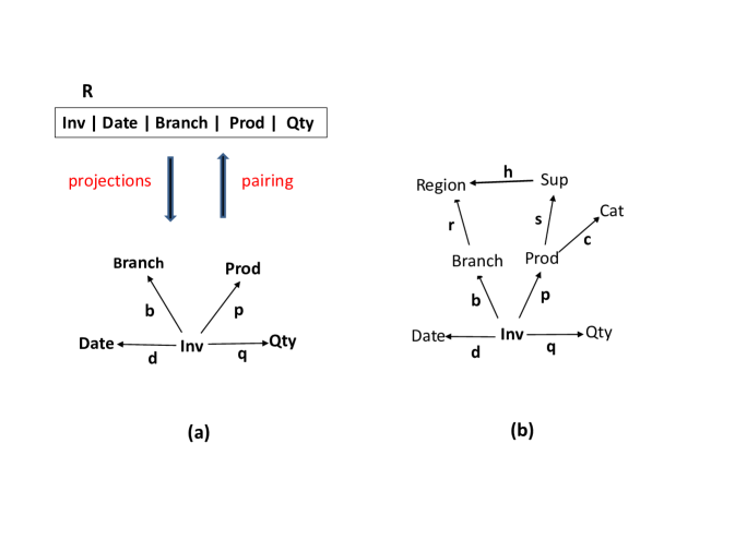
Figure 1: Example of context definition

As another example of context, suppose that, apart from the relation $R$, we have three more relations defined as follows:

$R1(Branch,Region)$ with $Branch$ as key

$R2(Prod,Sup,Cat)$ with $Prod$ as key

$R3(Sup,Region)$ with $Sup$ as key

The relation $R1$ gives for each branch the region where the branch is located; the relation $R2$ gives for each product the supplier and category of that product; and the relation $R3$ gives for each supplier the region in which its seat is located. Following the same reasoning as for $R$, we can associate $R1$ with the context $\{Branch\to Region\}$, $R2$ with the context $\{Prod\to Sup,Prod\to Cat\}$ and $R3$ with the context $\{Sup\to Region\}$. These three contexts put together with the context of $R$ make up the context shown in Figure 1(b).

Another way to look at the context shown in Figure 1(b) is to think of it as an ‘evolution’ of the context in Figure 1(a) in the sense that we have added the region in which each branch is located; the category and the supplier of each product; and the region in which each supplier has its seat. In other words, we can model this application independently of its relational representation.

Incidentally, note that the new edges added to the context of Figure 1(a), namely $r$, $c$, $s$ and $h$ can be seen as ‘derived’ edges in the sense that they can be computed from existing data. Indeed, the region of each branch can be computed (by Geo-localization) from the address of the branch; the region of each supplier from the address of supplier’s seat; and the category and supplier of each product can be ‘read off’ the code bar of the product. Note that this context has two ‘parallel paths’ from $Inv$ to $Region$ (‘parallel’ in sense ‘same source same target’).

By the way, the context of Figure 1(b) could be the context of a data warehouse with fact table $R$ and dimension tables $R1,R2,R3$.

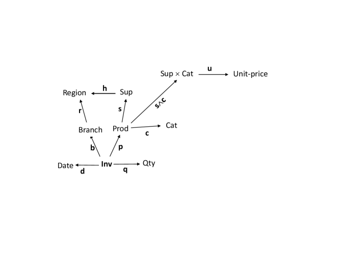
Figure 2: Representing the dependency $\{Sup,Cat\}\to Unitprice$

As a last example, consider the context of Figure 1(b) and suppose that the price of a product is determined by the supplier and the category of the product. In the relational model this is expressed by the functional dependency $\{Sup,Cat\}\to Unitprice$. To express this dependency in our model we need to add the edges $s\wedge c:Prod\to Sup\times Cat$ and $(Sup\times Cat)\to Unitprice$ as shown in Figure 2.

It should be evident from our examples that the model that we propose here is a graph database model DBLP:reference/bdt/GutierrezHW19 . A graph database model is a schema-less model that uses nodes, relationships between nodes and key-value properties instead of tables to represent information. Therefore it is typically substantially faster for associative data sets. While other database models compute relationships expensively at query time, a graph database stores connections as first-class citizens, readily available for any “join-like” navigation operation. Any purposeful query can be easily answered via graph databases, as data is easily accessed using traversals. A traversal is how you query a graph, navigating from starting nodes to related nodes according to an algorithm DBLP:journals/corr/AnglesABHRV16 . As we shall see, the functional algebra that we use in our model provides the basis for querying the database using such traversals.

There is a substantial body of literature around the use of graphs in computer science, including several tools to support graph management by means of digital technology, as well as data models and query languages based on graphs. The reader is referred to DBLP:conf/sigmod/ArenasGS21 DBLP:conf/aib/Hogan22 DBLP:journals/csur/HoganBCdMGKGNNN21 for a comprehensive analysis of graph-based approaches to data and knowledge management, emphasizing the relation between graph databases and knowledge graphs and including an extensive bibliography. A rather detailed discussion on the power and limitations of graph databases can be found in DBLP:conf/cisim/Pokorny15 . Moreover, several graph database systems have appeared in recent years such as Neo4j Graph Database, ArangoDB, Amazon Neptune, Dgraph and a host of others.

The main contributions of this paper are as follows: (a) we introduce a novel graph database model, called the context model, (b) we show that a consistent relational database can be embedded in the context model as a view over the context induced by its functional dependencies, (c) we define analytic queries in the query language of a context in a seamless manner - in contrast to the relational model where analytic queries are defined outside the relational algebra, and (d) we show that the context model can be used as a user-friendly interface to relational databases for data analysis purposes.

The remaining of the paper is organized as follows. In Section 2 we present the formal context model, namely the formal definition of context and database over a context, the query language of a context, and the notions of ‘view’ and ‘path-equality constraint’. In Section 3 we illustrate the expressive power of the context model by showing how a consistent relational database can be embedded in the context model; and how the context model can be used as a user-friendly interface to a relational database for data analysis purposes. And finally, in Section 4, we offer concluding remarks and discuss perspectives of our work.

2 The formal model

In this section we build upon the work of DBLP:conf/fqas/Spyratos06 , SpyratosS18 to give the formal definition of context and of database over a context; and then we define the query language of a context and the notions of ‘view’ and ‘path equality constraint’ over a context.

2.1 The definition of context

As we have seen informally in the introduction, a context is just a labeled directed graph in which each node represents a dataset and each edge $f$ from a node $X$ to a node $Y$ represents a function from the dataset $X$ to the dataset $Y$. We have also seen that a node of a context can be either a simple node such as $Branch$ or $Price$ in Figure  2, or a product node such as $Sup\times Cat$ in that same figure.

Let us now introduce informally some auxiliary concepts that we need in order to justify the formal definition of context. First, the dataset represented by a simple node $A$ comes always from a given, fixed set of values associated with $A$; this set is called the domain of $A$, denoted as $dom(A)$. Although the domain of a node $A$ can be an infinite set, $A$ always represents a finite set of values from its domain. As for a product node $A\times B$ its domain is defined as the product of the domains of $A$ and $B$ that is $dom(A\times B)=dom(A)\times dom(B)$.

Second, a context being a graph, it may contain cycles. However, we can convert a context into an acyclic graph by (a) showing that all nodes in a cycle are equivalent and (b) coalescing all nodes in every cycle to a single node.

To define the sense in which all nodes of a cycle are equivalent, define the following relation over nodes $X$ and $Y$ of a cycle: $X\equiv Y$ if there is a path from $X$ to $Y$. This relation is an equivalence relation as it is reflexive, symmetric and transitive. It follows that all nodes in a cycle are equivalent and therefore we can coalesce them into a single node (a representative of the cycle).

A typical example where cycles occur is when the price of a product is given in two (or more) different currencies, for example in dollars and in pounds, call them $\$Price$ and $\pounds Price$, respectively. In this case, we have the edges $\$Price\to\pounds Price$ and $\pounds Price\to\$price$ that represent ‘conversion functions’ from the price in dollars to the price in pounds and vice-versa. The existence of these edges makes the two nodes equivalent. Therefore we can choose one of the two nodes as the representative of the equivalence class $\{\pounds Price,\$Price\}$. Incidentally, in this example, one could replace the two nodes by a third, new node $Price$; and if this new node was made clickable then the user could see the ‘hidden’ equivalent nodes by clicking on $Price$. In general, if we click on a node $X$ we see all nodes equivalent with $X$, or eventually the node $X$ itself if there are no node equivalent to $X$.

In view of the above discussion, we shall make the assumption that all nodes in a cycle are represented by one node therefore a context has no cycle of length more than one. Furthermore, we shall make the following assumptions:

- every node $X$ of a context is equipped with an edge $\iota_{X}:X\to X$, called the ‘identity edge’ of $X$ and representing the identity function on $X$

- every context contains a ‘terminal node’ $T$ such that $dom(T)$ is a singleton

- every node $X$ of a context is equipped with a ‘terminal edge’ $\tau_{X}:X\to T$ representing a constant function from $X$ to $T$

The reasons behind these assumptions will become clear in the following section, when we discuss analytic queries and their properties.

Definition 1 (Context)

Let $U$ be a set in which every element $A$ is associated with a set of values called the domain of $A$, denoted by $dom(A)$. A context over $U$ is a finite, labeled, directed, acyclic graph $\mathcal{C}$ such that:

• each node of $\mathcal{C}$ is either an element of $U$ or the Cartesian product of a finite set of elements of $U$

• every node $A$ of $\mathcal{C}$ is associated with a unique edge $\iota_{A}:A\to A$ from $A$ to $A$ called the identity edge of $A$

• there is a distinguished node $T$ with no outgoing edges called the terminal node of $\mathcal{C}$

• every node $A$ of $\mathcal{C}$ is associated with a unique edge $\tau_{A}:A\to T$ called the terminal edge of $A$

• every node of $U$ is either source or target of an edge of $\mathcal{C}$ other than an identity edge (i.e., no isolated nodes)

Several remarks are in order here to clarify the above definition of context. First, although acyclic, a context is not necessarily a tree. In particular, a context can have more than one root as in Figure 3, and it can have parallel paths as in Figure 1(b). Here, the term ‘parallel paths’ is used to mean paths with the same source and same target. More formally, seen as syntactic objects, the edges of a context are triples of the form (source, label, target), therefore two edges are different if they differ in at least one component of this triple. This implies, in particular, that two edges can have the same label if they have different sources and/or different targets. Moreover, two different edges can have the same source and the same target as long as they have different labels. We call such edges parallel edges. Incidentally, it is because of the possibility of having parallel edges that we require that edges be labelled in the above definition.

Second, as we shall see in the next section, the presence of the terminal node $T$ in a context and of a terminal edge $\tau_{X}$ for each node $X$ are indispensable for expressing some important types of analytic queries.

Third, each node of a context will be assumed equipped with its identity edge, its terminal edge and with its projection edges (if the node is a product node). In our examples, however, we will not show these special edges if not necessary, but we will always assume their existence. In other words, every simple node $A$ will be assumed equipped with its identity edge $\iota_{A}$ and its terminal edge $\tau_{A}$ and every product node $A\times B$ will be assumed equipped with its identity edge $\iota_{A\times B}$, its terminal edge $\tau_{A\times B}$ and its projection edges $\pi_{A},\pi_{B},\pi_{AB}$ none of which will be shown but all of which will be assumed to be available at node $A\times B$ (and similarly if the node is the product of more than two factors). Note that we can consider a simple node $A$ as a trivial product node with only one factor, equipped with its identity edge $\iota_{A}$, its terminal edge $\tau_{A}$ and its (only) projection function: $\pi_{A}=\iota_{A}$.

Finally, a context can be seen as the interface between users of an application and the datasets of the application, in the sense that users formulate their queries using the nodes and edges of the context. Therefore a context plays the role of a schema. However, in contrast to, say, a relational schema, a context is not aware of complex structures in data. For example, a context is not aware of how functions might be grouped together into relations. It is the query language that gives the possibility to users to create such complex structures. We shall come back to this remark in the following section when we describe how a relational database can be defined as a view over the context induced by its functional dependencies.

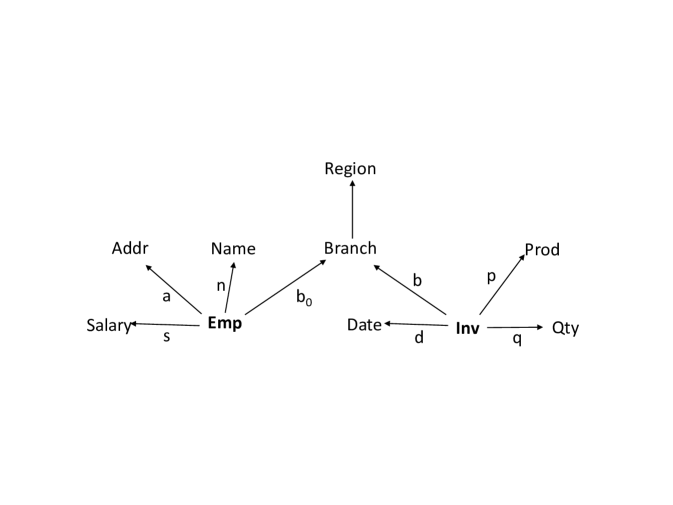
Figure 3: A context with two roots

Now, a context is a syntactic object and its nodes and edges can be associated with data values as discussed in the introduction. These associations constitute what we call a database over a context.

Definition 2 (Database)

Let $\mathcal{C}$ be a context. A database over $\mathcal{C}$ is a function $\delta$ from nodes and edges of $\mathcal{C}$ to sets of values such that:

• for each simple node $A$ of $\mathcal{C}$, $\delta(A)$ is a finite subset of $dom(A)$

• for each product node $A\times B$, $\delta(A\times B)=\delta(A)\times\delta(B)$; and similarly for the product of more than two nodes.

• for each edge $f:X\to Y$ of $\mathcal{C}$, $\delta(f)$ is a total function from $\delta(X)$ to $\delta(Y)$

• for each simple node $A$ of $\mathcal{C}$, $\delta(\iota_{A})$ is the identity function on $\delta(A)$; and as a consequence, $\delta(\iota_{A\times B})((a,b))=(\iota_{A}(a),\iota_{B}(b))$, for all $(a,b)$ in $\delta(A\times B)$; and a similar argument holds for the product of more than two nodes.

• $\delta(T)$ is a singleton.

Several remarks are in order here regarding this definition of database. First, in our discussions if $X$ is a node, we shall refer to $\delta(X)$ as the current instance or the extension of $X$; and and if $f$ is an edge, we shall refer to $\delta(f)$ as the current instance or the extension of $f$. Moreover, in order to simplify our discussions, we shall confuse the terms ‘node $X$’ and ‘current instance of $X$’, the terms ‘edge $f$’ and ‘current instance of $f$’ and the terms ‘path $p=f_{1};\ldots;f_{n}$’ and ‘function $\delta(p)=\delta(f_{n})\circ\dots\circ\delta(f_{1})$’ when no ambiguity is possible. Indeed, more often than not, the intended meaning will be evident from the use of these terms. For example, if $e$ is an edge and we write $e^{-1}$ this will clearly mean $\delta(e)^{-1}$; and similarly, if $e:X\to Y$ and $f:Y\to Z$ are two edges and we write $f\circ e$ this will clearly mean the composition $\delta(f)\circ\delta(e)$.

Second, as the data assigned by $\delta$ to an edge $f:X\to Y$ of a context is a function, and as the current instances of $X$ and $Y$ are finite so will be the current instance of $f$. Therefore $\delta(f):\delta(X)\to\delta(Y)$ is a finite function. Moreover, in this definition, we assume that $\delta(f)$ is a total function that is $\delta(f)$ is defined on every value of $\delta(X)$ which means that we assume no nulls.

Third, as the terminal node is assigned a singleton set, the function $\delta(\tau_{X}):\delta(X)\to\delta(T)$ is a constant function, for every node $X$. Note that we may use any name for the single element of $\delta(T)$. For the purposes of this paper however we choose the name All that is we define $\delta(T)=\{All\}$, where All is a constant. The reason why we choose this name is because All is a reminder of the fact that $\delta(\tau_{X})^{-1}(All)=\delta(X)$ (i.e, the inverse of function $\tau_{X}$ is the whole set $\delta(X)$). We shall come back to this remark when we define analytic queries in the following section.

2.2 The query language of a context

In order to access the data of a context users need operations to combine nodes and edges so as to formulate queries. In our model we use one operation to combine nodes, namely the Cartesian product, and three operations to combine functions, namely composition of two or more functions, restriction of a function to a subset of its domain of definition and pairing of two or more functions (as defined in the introductory section). These four operations on nodes and edges are well known, elementary operations that we call collectively the functional algebra of a context.

Definition 3 (Functional algebra)

Given a context $\mathcal{C}$, the functional algebra of $\mathcal{C}$ consists of the following operations:

• Cartesian product of two or more nodes

• Restriction of a function to a subset of its domain of definition

• Composition of two or more functions

• Pairing of two or more functions with the same source.

It is worth noting here that the four operations of the functional algebra are strongly connected to each other as stated in the following lemma. Its proof is a direct consequence from the definitions of the above operations (see also Figure 4).

Lemma 1

Let $X,Y,Z$ be three nodes of a context $\mathcal{C}$ and $f:X\to Y$ and $g:X\to Z$ be two edges of $\mathcal{C}$. Then the following hold: $\pi_{Y}(f\wedge g)=f$ and $\pi_{Z}(f\wedge g)=g$.

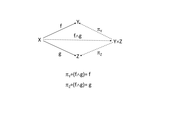
Figure 4: Illustrating lemma 1

There is an interesting ‘derived’ operation, whose definition uses operations of the functional algebra. This operation is called ‘product’ of two or more functions

Definition 4 (Product of functions)

Let $f:X\to Y$ and $g:X^{\prime}\to Y^{\prime}$ be two functions. The product of $f$ and $g$ is a function $f\times g:X\times X^{\prime}\to Y\times Y^{\prime}$ defined as follows:  $(f\times g)=(f\circ\pi_{X})\wedge(g\circ\pi_{X^{\prime}})$
In other words:

$(f\times g)(x,x^{\prime})=((\pi_{X}\circ f)(x,x^{\prime}),(\pi_{X^{\prime}}\circ g)(x,x^{\prime}))$, for all $(x,x^{\prime})$ in $X\times X^{\prime}$.

Clearly, the above definition of product can be extended to more than two functions in a straightforward manner.

Note that there is an alternative but equivalent definition of product which is sometimes preferable to use instead of the above definition:

Definition 5

Let $f:X\to Y$ and $g:X^{\prime}\to Y^{\prime}$ be two functions. The product of $f$ and $g$ is a function $f\times g:X\times X^{\prime}\to Y\times Y^{\prime}$ defined as follows:  $(f\times g)((x,x^{\prime}))=(f(x),g(x^{\prime})),$ for all $(x,x^{\prime})$ in $X\times X^{\prime}$.

Now, every well-formed expression of the functional algebra of a context $\mathcal{C}$ represents a query over $\mathcal{C}$. For example, in the context of Figure 2, the expression $r\circ b$ is a query ‘asking’ for the set of pairs $(Inv,Region)$, and similarly $s\wedge c$ is a query asking for the set of triples $(Prod,Sup,Cat)$.

Definition 6 (Query language)

Let $\mathcal{C}$ be a context. A query $Q$ over $\mathcal{C}$ is one of the following:

• a Cartesian product of nodes of $\mathcal{C}$

• an edge of $\mathcal{C}$ or a well-formed expression whose operands are nodes and edges of $\mathcal{C}$ and whose operations are among those of the functional algebra.

Definition 7 (Query answer)

Let $\mathcal{C}$ be a context, $\delta$ a database over $\mathcal{C}$ and $Q$ a query over $\mathcal{C}$. The answer of $Q$ in $\delta$ is the function obtained after replacing the operands of $Q$ with their current instances and performing the operations.

Therefore, if the query is a Cartesian product of nodes, say $A\times B$, then the answer is the Cartesian product $\delta(A)\times\delta(B)$. Otherwise, if the query is an edge, say $e:X\to Y$, then the answer is the function $\delta(e):\delta(X)\to\delta(Y)$; and if the query is a well-formed expression involving two or more edges then the answer is the function obtained after replacing each operand $e$ in the query by its extension $\delta(e)$ and performing the operations. In this case, the source and the target of the answer can be defined recursively based on the sources and targets of the edges appearing in the query. For example, in Figure 2, if $Q_{1}=r\circ b$ then $source(Q_{1})=Inv$ and $target(Q_{1})=Region$; and similarly, if $Q_{2}=(r\circ b)\wedge p$ then $source(Q_{2})=Inv$ and $target(Q_{2})=Region\times Product$.

Let us see a few examples of queries using the context of Figure 2. The simplest query is a single edge, for example $Q1=b$. Its answer is the current instance of $e$, namely $Ans(Q1)=\delta(b)$ and can be represented as a set of pairs:

$Ans(Q1)=\{(x,y)/x\in\delta(Branch),y=\delta(b)(x)\}$

Therefore the answer can be represented as a relation $R1(Branch,Region)$, in the sense of the relational model; and this relation satisfies the dependency $Branch\to Region$ since $\delta(b):\delta(Branch)\to\delta(Region)$ is a function.

As another example consider the query $Q2=(h\circ s)\wedge c$. Its answer is the function $Ans(Q2)=(\delta(h)\circ\delta(s))\wedge\delta(c)$ and can be represented as a set of triples:

$Ans(Q2)=\{(x,y,z)\}/x\in\delta(Prod),y=(\delta(h)\circ\delta(s))(x),z=\delta(c)(x)\}$.

Therefore, again, the answer can be represented as a relation $R2(Prod,Region,Cat)$, in the sense of the relational model, satisfying the dependencies $Prod\to Region$ and $Prod\to Cat$ since $\delta(h)\circ\delta(s):\delta(Prod)\to\delta(Region)$ and $\delta(c):\delta(Prod)\to\delta(Cat)$ are functions.

A more tricky example now is the following query: $Q3=(h\circ s\circ p)\wedge(r\circ b)$. Its answer is the function

$Ans(Q3)=((\delta(h)\circ\delta(s)\circ\delta(p))\wedge(\delta(r)\circ\delta(b))$

and can be represented as a set of triples:

$Ans(Q3)=\{(x,y,z)/x\in\delta(Inv),y=(\delta(h)\circ\delta(s)\circ\delta(p))(x),z=(\delta(r)\circ\delta(b))(x))\}$

Note that both values $y$ and $z$ are branches. However, there is no ambiguity between $y$ and $z$ as they are computed by two different functions: given an invoice $x$, $y$ is the region where the supplier’s seat is located (computed by $\delta(h)\circ\delta(s)\circ\delta(p)$) and $z$ is the region where the branch is located (computed by $\delta(h)\circ\delta(s)\circ\delta(p)$). Representing this information in the relational model requires two ‘renamings’ of the attribute $Region$, namely $Branch.Region$ and $Sup.Region$, to represent the two different values $y$ and $z$ (in general, one needs as many renamings as there are different paths to $Branch$). Clearly, this is the cost to pay if one wants to represent data and query results in usual (1NF) tables as is the case in the relational model. In contrast, in our model, there is no need for renamings: if we want to represent query results in usual (1NF) tables then each column of the table can be labeled by the path computing the values of the column.

The above examples of queries use composition and pairing. Regarding the use of restriction, let us consider the following possible cases: $(i)$ the query is a single path and $(ii)$ the query is the pairing of two or more paths.

First suppose that the query is a single path, say $f:X\to Y$ and $g:Y\to Z$. If node $X$ is restricted to a subset $E$ then the answer is computed by the composition $g\circ(f/E)$. If moreover $Y$ is restricted to a subset $F$ then we can compute the answer by (a) ‘pushing’ the restriction of $Y$ to $X$ by defining $E^{\prime}=E\cap g^{-1}(F)$ and (b) computing the answer as $g\circ(f/E^{\prime})$. As it should be obvious from these examples, if the query is a single path then we can ‘push’ the restriction of any node along the path to the source of the path. On the other hand, if the query is the pairing of two or more paths, say $p_{1},\ldots,p_{n}$ with (common) source $X$ then we can proceed as follows: (a) let $E_{i}$ be the result of ‘pushing’ the node restrictions of path $p_{i}$ to $X$, $i=1,\ldots,n$, (b) if $E$ is the restriction of the source node $X$ then define $E^{\prime}=E\cap E_{1}\cap\ldots\cap E_{n}$ and (c) compute the pairing with $X$ restricted to $E^{\prime}$. We note that restricting the nodes of a query corresponds to the ‘selection’ operation in relational algebra queries (hence to the ‘where’ clause of SQL).

An important class of queries is the one in which each query is the pairing of one or more paths with common source, such as the queries $Q1,Q2$ and $Q3$ above. We call such queries ‘subcontext queries’.

Definition 8 (Subcontext query and tree query)

Let $\mathcal{C}$ be a context. A subcontext query $Q$ over a set of nodes $A_{1},\ldots,A_{n}$ is defined by giving a node $K$ and at least one path from $K$ to $A_{i}$, $i=1,\ldots,n$. The node $K$ is called the key, the nodes $A_{1},\ldots,A_{n}$ the attributes, and the paths from $K$ to $A_{i}$, $i=1,\ldots,n$, the attribute paths of $Q$. If there is exactly one path from $K$ to $A_{i}$, $i=1,\ldots,n$, then $Q$ is called a tree query.

Note that, in the above definition of subcontext and tree query, the key $K$ can be a simple node like $Inv$ or $Region$ in Figure 2, or a product node like $Prod\times Cat$ in that same figure; and similarly, each $A_{i}$ can be a simple node or a product node. However, if a node $A_{i}$ is a product node, say $A\times B$, we can always replace the path $p:K\to A\times B$ by the two paths $\pi_{A}\circ p:K\to A$ and $\pi_{B}\circ p:K\to B$, based on Lemma 1. Therefore, without loss of generality, we can assume that each $A_{i}$ in the above definition is a simple node (and we shall make this assumption in this paper in order to simplify our discussions).

Let us illustrate this definition using the context of Figure 1(b). We can define a subcontext query $\mathcal{S}$ over $Region$ and $Cat$ by designating $Inv$ as the key and giving two paths from $Inv$ to $Region$, namely: $Inv\to Branch\to Region$ and $Inv\to Prod\to Sup\to Region$; and one path from $Inv$ to $Cat$, namely: $Inv\to Prod\to Cat$. Note that the two paths from $Inv$ to $Region$ are parallel paths.

As another example, we can define a tree query $S_{1}$ over the nodes $Region$ and $Cat$ by designating $Inv$ as the key and the paths $Inv\to Branch\to Region$ and $Inv\to Prod\to Cat$ as the attribute paths; and as yet another example, we can define the tree query $\mathcal{S}_{2}$ over $Sup$ and $Cat$ by designating the node $Prod$ as the key and the paths $Prod\to Sup$ and $Prod\to Cat$ as the attribute paths. Note that we can define a different tree query $\mathcal{S}_{3}$ over the same nodes, $Sup$ and $Cat$, by designating the node $Inv$ as the key and the paths $Inv\to Prod\to Sup$ and $Inv\to Prod\to Cat$ as the attribute paths. Clearly, although $\mathcal{S}_{2}$ and $\mathcal{S}_{3}$ are defined over the same nodes, they have different semantics.

The term ‘subcontext query’ is justified by the fact that all its edges belong to $\mathcal{C}$, therefore the query is a context rooted in $K$.

The importance of this class of queries lies in the fact that their answers can be represented as relations satisfying the dependencies that were used in their definition (this is obvious in queries $Q1,Q2$ and $Q3$ above).

The important characteristic of a tree query, in particular, lies in the fact that we can represent both, the query and its answer by a usual table. Indeed, let $\mathcal{C}$ be a context and let $Q$ be a tree query over nodes $A_{1},\ldots,A_{n}$ with key $K$ and attribute paths $p_{1},\ldots,p_{n}$. Let $\delta$ be a database over $\mathcal{C}$ and let Ans($Q$) be the answer to $Q$ with respect to a database $\delta$. Then Ans($Q$) can be represented by a table whose columns are indexed by the nodes $K,A_{1},\ldots,A_{n}$, rows are indexed by the values in $\delta(K)$, and for each value $k\in\delta(K)$ the cell $(k,A_{i})$ contains the value $\delta(p_{A_{i}})(k)$. As there is only one path $p_{A_{i}}$ from $K$ to $A_{i}$, it follows that each cell contains one and only one value. In the relational model such a table is said to be in First Normal Form ($1NF$ for short, see Ullman ). Therefore a tree query as defined above returns a relation (in the sense of the relational model) which is in First Normal Form and whose key is $K$. Additionally, this relation is consistent (in the sense of the relational model) that is the projection of the table over $KA_{i}$ is a function, for all $i=1,\ldots,n$, and this function is $\delta(p_{A_{i}})$, $i=1,\ldots,n$.

Clearly, the above representation of the answer to a tree query $Q$ by a table in $1NF$ is still valid if $Q$ is a subcontext query, provided that all parallel paths in $Q$ between $K$ and $A_{i}$ are assigned the same function by $\delta$, $i=1\ldots,n$. We shall come back to these remarks concerning tree queries and subcontext queries in the following section.

Fourth, a database over a context $\mathcal{C}$ can be seen as assigning ‘semantics’ to the nodes and edges of $\mathcal{C}$. Note that, under this view, two tree subcontexts over the same set of nodes may receive different semantics. For example, the tree queries $\mathcal{S}_{2}$ and $\mathcal{S}_{3}$, defined earlier, both over nodes $Sup$ and $Cat$, have different semantics. Indeed, in every database over $\mathcal{C}$, all products appearing in the answer to $\mathcal{S}_{3}$ also appear in the answer of $\mathcal{S}_{2}$ whereas the opposite is not true.

A last remark regarding contexts, databases and queries is the following. A context describes the functioning of an enterprise as seen by a domain expert, while a database over the context records the current data of the enterprise. As for the query language, it helps extract information on the current status of the enterprise. What we would like to stress here is that defining a context is one thing while designing queries to extract useful information is quite another thing. For example, consider the following trivial context: $\mathcal{C}=\{f:Emp\to Dep,g:Prod\to Price\}$. The queries $Q1=f$ and $Q2=g$ ‘make sense’ as they return each employee’s department and each product’s price, respectively. In contrast, the query $Q3=f\times g$ makes little sense as it puts together employee-product pairs and the corresponding department-price pairs. In other words, defining what is useful can’t be automated and designing a set of queries useful to the functioning of an enterprise is not an easy job.

2.3 View of a context

A user or a group of users may want to use only a part of the information contained in a context, and may want that part to be structured again as a context, reflecting specific user needs. For example, Figure 5 shows a context $\mathcal{C}$ and two views of $\mathcal{C}$, namey $\mathcal{V}_{1}$ and $\mathcal{V}_{2}$. Each node of $\mathcal{V}_{1}$ appears in $\mathcal{C}$ and the edges $e,e^{\prime}$ of $\mathcal{V}_{1}$ are defined as queries over $\mathcal{C}$. In other words, $\mathcal{V}_{1}$ is a context whose nodes and edges are queries over $\mathcal{C}$ (and similarly for $\mathcal{V}_{2}$).

Definition 9 (View of a context)

Let $\mathcal{C}$ be a context. A view of $\mathcal{C}$ is defined to be a context $\mathcal{V}$ whose nodes and edges are queries over $\mathcal{C}$. Given a database $\delta$ over $\mathcal{C}$ the current instance of $\mathcal{V}$ is defined to be the set of answers to the queries defining the nodes and edges of $\mathcal{C}$.

It should be clear that the concept of view as well as the problems related to view management in our approach are similar to those in the relational model: a view can be virtual or materialized; a query over a virtual view $\mathcal{V}$ must be translated into a query over the context $\mathcal{C}$ in order to be answered whereas a query in a materialized view can be answered directly from the view; when the database over the context $\mathcal{C}$ is updated, the updates are propagated to the view only if the view is materialized; updating through views is problematic; and so on (see Ullman ).

As an example consider the view $\mathcal{V}_{1}$ in Figure 5 and consider the following query over that view: $Q=e\wedge e^{\prime}$. To answer $Q$, $e$ and $e^{\prime}$ are replaced by their definitions to obtain the query $\overline{Q}=(r\circ b)\wedge(c\circ p)$ which is evaluated over $\mathcal{C}$ to obtain the answer to $Q$. Note that, as this example shows, the edges of a view of a context $\mathcal{C}$ can be seen as macros that facilitate the formulation of queries over $\mathcal{C}$.

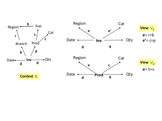
Figure 5: A context $\mathcal{C}$ and two views of $\mathcal{C}$ with different roots

2.4 Path equality constraints

As we have seen, a context is an acyclic graph (up to node equivalence) in which we may have more than one root and we may also have parallel paths. For example, in Figure 3 we have two roots, $Emp$ and $Inv$, and two parallel paths from node $Inv$ to node $Region$.

Now, in a database $\delta$, if we compose the edges along two or more parallel paths then we obtain functions with the same source and the same target. In the example of Figure 1(b) these functions are:

$e=r\circ b:Inv\to Region$ and $e^{\prime}=u\circ b\circ p:Inv\to Region$

In general, such ‘parallel functions’ do not have to be equal. However, in our model, we can use their equality in two important ways: (a) to express conditions in queries and (b) to express constraints that a database over a context must satisfy. For example, consider the following queries over the context of Figure 1(b):

$Q1=\pi_{Sup,Region}(e\wedge e^{\prime})$

$Q2=\pi_{Sup,Region}((e\wedge e^{\prime})/E)$, where $E=\{i\in Inv/e(i)=e^{\prime}(i)\}$

If the database is unconstrained then $Q1$ returns a set of pairs $(Sup,Region)$ which may contain pairs $(Sup,Region)$ such that the supplier’s region is not the same as the branch’s region; whereas $Q2$ returns a pair $(Sup,Region)$ only if the supplier’s region is ‘equal’ (ı.e., the same) as the branch’s region. If the database is constrained to satisfy all path equalities then $Q1$ and $Q2$ both return the same answer.

The above discussion motivates the following definition of path equality constraint.

Definition 10

Let $\mathcal{C}$ be a context. A pair $(p,p^{\prime})$ of parallel paths of $\mathcal{C}$ is called a path equality constraint over $\mathcal{C}$. A database $\delta$ over $\mathcal{C}$ is said to satisfy $(p,p^{\prime})$, denoted $\delta\models(p,p^{\prime})$, if $\delta(p)=\delta(p^{\prime})$. Moreover, $\delta$ is said to be consistent with respect to a set $PP$ of equality constraints, denoted by $\delta\models PP$, if it satisfies all path equalities of $PP$. Finally, $\delta$ is said to be consistent over $\mathcal{C}$ if it satisfies all equality constraints of $\mathcal{C}$.

It is important to note that in a consistent database every set of parallel functions is actually replaced by a single function, and therefore the set of functions of a consistent database is a tree (or a set of trees if the context has more than one root). In this case every set of parallel edges in the underlying context $\mathcal{C}$ can be replaced by a single edge to obtain a tree (or a set of trees if $\mathcal{C}$ has more than one root).

Following this remark, an interesting question is: can we replace the database tree by a set of trees of height one without loss of database content and/or without loss of equality constraints?

The interest in answering this question lies in the fact that each tree of height one can be represented as a table whose rows are indexed by the root of the tree, say $K$, and whose columns are indexed by the leaves, say $A_{1},\ldots,A_{n}$. Indeed, such a tree is of the form $f_{A_{i}}:K\to A_{i}$, $i=1,\ldots n$ and can be represented by a table whose rows are indexed by the values of $K$ and whose columns are indexed by $A_{1},\ldots,A_{n}$; and for each value $k$ of $K$ the cell $<k,A_{i}>$ contains the value $f_{A_{i}}(k)$. In other words, in this case, the database can be represented by a set of tables, thus providing a user-friendly interface to the database content. Moreover, one can design easy to use languages for accessing the database content (such as the SQL language).

This kind of ‘decomposition’ into a set of trees of height one together with a number of related questions lie outside the scope of the present paper and it is the subject of future work.

3 Applications

In this section, we answer two important questions: (a) how to embed a consistent relational database as a view of a context and (b) how to use the context model as a user-friendly interface to a relational database for data analysis purposes.

3.1 Embedding relations in a context

Let $R(A_{1},\ldots,A_{n})$ be a relation schema with a set $FD$ of functional dependencies over the attribute set $U=\{A_{1},\ldots,A_{n}\}$. We recall that two subsets $X,Y$ of $U$ are equivalent if the dependencies $X\to Y$ and $Y\to X$ are both implied by $FD$. It follows that all keys of $R$ are equivalent and let’s call $K$ the unique key of $R$ (up to equivalence). Then the dependency $K\to X$ is implied by $FD$ for every subset $X$ of $U$ and let’s define:

$FD^{\prime}=FD\cup\{K\to X/X\subseteq U\}$

Let us now consider a relation $r$ over $R$ and define: $\delta(X)=\pi_{X}(r)$ for every subset $X$ of $U$. Moreover, for every dependency $f:X\to Y$ in $FD^{\prime}$, where $X,Y$ are subsets of $U$, let’s define $\delta(f):\pi_{X}(r)\to\pi_{Y}(r)$ such that: for every tuple $t$ in $r$, $\delta(f)(t.X)=t.Y$. If $r$ is consistent then we have the following facts:

Fact 1: As $r$ is consistent, $\delta(f)$ is a function, for every $f$ in $FD^{\prime}$ (by the definition of consistency); and moreover, $\delta(f)$ is a total function over $\pi_{X}(r)$.

Fact 2: As $r$ is in $1NF$, for every $f:X\to Y$ in $FD$ we have that: $f\circ\delta(K\to X)=\delta(K\to Y)$ (otherwise there would exist a value $k$ in $\delta(K)$ such that $f\circ\delta(K\to X)(k)\neq\delta(K\to Y)(k)$), thus violating $1NF$.

Fact 3: $r=\delta(K\to A_{1})\wedge\ldots\wedge\delta(K\to A_{n})$, where ‘$\wedge$’ is the operation of pairing of functions with common source (here, the common source is $K$).

It can be easily seen that:

$FD^{\prime}$ is a context, call it $\mathcal{C}_{FD^{\prime}}$, rooted in $K$ and $\delta$ is a database over $\mathcal{C}_{FD^{\prime}}$

$R=(K\to A_{1})\wedge\ldots\wedge(K\to A_{n})$ is a subcontext query over $\mathcal{C}_{FD^{\prime}}$ and $Ans(R)=r$. In other words $R$ is a view of $\mathcal{C}_{FD^{\prime}}$.

It follows that a consistent relational database $\{R_{1},\ldots,R_{m}\}$ can be seen as a view of the context $FD_{R_{1}}^{\prime}\cup\ldots\cup FD_{R_{m}}^{\prime}$ satisfying all its parallel paths (i.e. all pairs of paths of the form $K\to X\to Y$ and $K\to Y$).

An important remark is in order here. The requirement of the relational model that the relations in a database be in First Normal Form has two important consequences: (a) it reduces the expressive power of the model as opposed to the context model and (b) it introduces ambiguity in the interpretation of query answers.

Let us explain these claims using a simple example. Suppose that we want to design a relational database schema over a universe $U=\{Emp,Dep,Mgr\}$ with a set $FD=\{f:Emp\to Dep,g:Dep\to Mgr,h:Emp\to Mgr\}$ meaning that an employee works for one and only one department, a department has one and only one manager, and an employee has one and only one manager - who may not be the employee’s department manager. In other words, although parallel, the two paths $Emp\to Dep\to Mgr$ and $Emp\to Mgr$ do not necessarily represent two equal functions in a database.

Clearly, putting all three attributes, $Emp,Dep$ and $Mgr$ in a single relation schema $R$ is not an option as relations over $R$ would not be in First Normal Form. The solution proposed in the relational model is to (a) ‘decompose’ $R$ by putting the dependencies $f$ and $g$ in one schema, say $R_{1}$ and the dependency $h$ in a different schema, say $R_{2}$; and (b) to rename the attribute $Mgr$ as $Dep.Mgr$ in $R_{1}$ and as $Emp.Mgr$ in $R_{2}$.

Although this solution seems reasonable in terms of data representation, it still has a problem when it comes to interpreting query answers. For example consider the query $\pi_{Emp,Dep.Mgr}(R_{1})\cup R_{2}$ which returns employee - manager pairs. Given a tuple $(e,m)$ in the answer, we don’t know if $m$ is the manager of $e$ or the manager of $e$’s department. A similar ambiguity is introduced in the answer of queries using joins, for example in the answer of the query: $\pi_{Emp,Dep.Mgr}(R_{1})\bowtie R_{2}$.

In contrast, in our model, by representing directly the functions relating the datasets of an application and using a functional language to formulate queries, we have both, a clear representation of data and no ambiguity in query answers.

Indeed, as we explained in the previous section, a relation schema corresponds to a set $R$ of paths in a context, with common source $K$ and if we want it to be in First Normal Form then we require equality of all parallel paths in $R$. However, this requirement is not mandatory as we may very well combine relation schemas whose parallel paths are not equal, using the operations of the functional algebra. For instance, in our previous example, we can combine $R_{1}$ and $R_{2}$ using pairing: $(R_{1}\wedge R_{2})$, in which the paths $Emp\to Dep\to Mgr$ and $Emp\to Mgr$ are distinct factors of the pairing. Note that the two paths appear in the same ‘relation schema’ without ambiguity, although we do not require this schema to be in First Normal Form.

We can summarize our discussion above as follows:

- A relation schema $R(U)$ with a set $FD$ of dependencies corresponds to a subcontext query in the context $\mathcal{C}_{FD^{\prime}}$.

- If $R(U)$ is in $1NF$ then it corresponds to a tree query in the context $\mathcal{C}_{FD^{\prime}}$.

Our conclusion here is that the constraint that each relation in a relational database must be in First Normal Form reduces the expressive power of the relational model and introduces ambiguity in query answers. First Normal Form is after all a representational constraint, namely that all data should be representable by usual tables. Our proposal is the following: rather than having the database administrator design a set of relations with accompanying functional dependencies in $1NF$, give users the freedom to define their own relations the way they want and manipulate them using the functional algebra. In defining their relations, users can be aided from interfaces such as the one described in the next section.

Summarizing what we have seen in this section, we can say that we have demonstrated (a) that a consistent relation in $1NF$ can be represented as a tree query in the context induced by its functional dependencies and (b) that a non-$1NF$ relation can be represented as a subcontext query.

3.2 A context as an interface

In this section we show how a context can serve as a user-friendly interface to a relational database for data analysis purposes. The general idea works as follows: (a) represent the database by a context as explained in the introductory section (see Figure 1) and make its nodes clickable, (b) the user defines an analytic query over the context through a sequence of clicks that the interface translates as an SQL Group-by query on the underlying database and (c) the user receives the result in the form of a table and/or in a visual form following some visualization template. Our idea is depicted in the diagram of Figure 7 that we will elaborate further shortly.

We have already seen how to define a relation over a context as the answer of a tree query over nodes $A_{i},i=1,\ldots,n$ by designating a node $K$ (the key) and a single path $p_{i}$ from $K$ to each $A_{i}$, $i=1,\ldots,n$, where the $A_{i}$’s are called the attributes of $K$.

As for defining an analytic query over a context, we adopt the definition of SpyratosS18 that we recall briefly here, using the example that we have seen in the introduction (Figure 1(b)). This example concerns the set of all delivery invoices, say over a year, in a distribution center (e.g. Walmart) which delivers products of various types in a number of branches.

Each delivery invoice has an identifier (e.g. an integer) and shows the date of delivery, the branch in which the delivery took place, the type of product delivered (e.g. $CocaLight$) and the quantity (i.e. the number of units delivered of that type of product). There is a separate invoice for each type of product delivered, and the data on all invoices during the year is stored in a database for analysis and planning purposes.

Suppose now that we want to know the total quantity delivered to each branch during the year. This computation needs only two among the four functions, namely $b$ and $q$. Figure 6 shows a toy example of the data returned by $b$ and $q$, where the data-set $Inv$ consists of seven invoices, numbered 1 to 7. In order to find the total quantity by branch we proceed in three steps as follows:

Grouping: During this step we group together all invoices referring to the same branch (using the function $b$). We obtain the following groups of invoices (also shown in the figure):

• Branch $b_{1}$: $1,2$

• Branch $b_{2}$: $3,4$

• Branch $b_{3}$: $5,6,7$

Measuring: In each group of the previous step, we find the quantity corresponding to each invoice in the group (using the function $q$):

• Branch $b_{1}$: 200, 100

• Branch $b_{2}$: 200, 400

• Branch $b_{3}$: 100, 400, 100

Aggregation: In each group of the previous step, we sum up the quantities found:

• Branch $b_{1}$: $200+100=300$

• Branch $b_{2}$: $200+400=600$

• Branch $b_{3}$: $100+400+100=600$

Then the association of each branch to the corresponding total quantity, as shown in Figure 6, is the desired result:

• Branch-1 $\rightarrow 300$

• Branch-2 $\rightarrow 600$

• Branch-3 $\rightarrow 600$

We view the ordered triple $Q=(b,q,sum)$ in Figure 6 as an analytic query over the context, the function $Ans_{Q}:Branch\rightarrow TotQty$ in that same figure as the answer to $Q$, and the computations as the query evaluation process.

Note that what makes the association of branches to total quantities possible is the fact that $b$ and $q$ have a common source (which is $Inv$).

The function $b$ that appears first in the triple $(b,q,sum)$ and is used in the grouping step is called the grouping function; the function $q$ that appears second in the triple is called the measuring function, or the measure; and the function $sum$ that appears third in the triple is called the aggregate operation. Actually, the triple $(b,q,sum)$ should be regarded as the specification of an analysis task to be carried out over the dataset $Inv$.

Note that exchanging the two first component of this triple we obtain the query $(q,b,sum)$ which is not a well formed query as the aggregate operation is not applicable on b-values that are Branches (i.e. we can’t sum up branches). However if instead of ‘sum’ we put ‘count’ as the aggregate operation then we obtain the query $(q,b,count)$ which is a well formed query, as ‘count’ is an aggregate operation applicable on b-values. By the way, what this query returns is the number of branches which were delivered the same quantity of products.

To see another example of analytic query, suppose that $T$ is a set of tweets accumulated over a year; $dd$ is the function associating each tweet $t$ with the date $dd(t)$ in which the tweet was published; and $cc$ is the function associating each tweet $t$ with its character count, $cc(t)$. To find the average number of characters in a tweet by date, we follow the same steps as in the delivery invoices example: first, group the tweets by date (using function $dd$); then find the number of characters per tweet (using function $cc$); and finally take the average of the character counts in each group (using ‘average’ as the aggregate operation). The appropriate query formulation in this case is the triple $(dd,cc,avg)$.

As yet another example, consider the context of Figure 2. The query to find the total quantity delivered by region is the following: $(r\circ b,q,sum)$ and the query to find the total value of products delivered by supplier is:

$(s\circ p,u\circ(s\wedge c)\circ p,sum)$.

As a last example, consider again the context of Figure 2. The query to find the average quantity delivered by region and supplier is the following: $(r\wedge p,q,sum)$.

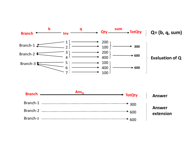
Figure 6: The evaluation of an analytic query

As we can see from these examples, the grouping function $g$ and the measuring function $m$ are each a functional expression. Therefore summarizing our discussion so far, we can say that an analytic query is defined to be an ordered triple $Q=(g,m,op)$ such that $g$ and $m$ are functional expressions with common source, say $K$, and $op$ is an aggregate operation applicable on $m$-values. The evaluation of $Q$ is done in three steps as follows: (a) group the items of $K$ using the values of $g$ (i.e. items with the same $g$-value $g_{i}$ are grouped together), (b) in each group of items, extract from $K$ the $m$-value of each item in the group, and (c) aggregate the $m$-values thus obtained (using $op$) to get a single value $v_{i}$. The value $v_{i}$ is defined to be the answer of $Q$ on $g_{i}$, that is $Ans_{Q}(g_{i})=v_{i}$. This means that a query is a triple of functions and its answer is also a function.

Clearly, given a context $\mathcal{C}$, we can use the identity edge $\iota_{X}$ and the terminal edge $\tau_{X}$ of a node $X$ in the same way as any other edge of $\mathcal{C}$. In particular, we can use them to form functional expressions and we can use such expressions in defining analytic queries. Referring to the context of Figure 1(b), here are two examples of analytic queries using these special edges $\iota_{A}$ and $\tau_{A}$:

$Q_{1}=(\iota_{Inv},q,sum)$ and $Q_{2}=(q,\iota_{Inv},count)$

During the evaluation of $Q_{1}$, in the grouping step, the function $\iota_{Inv}$ puts each invoice of $Inv$ in a single block. Therefore summing up the values of $q$ in a block simply finds the value of $q$ on the single invoice in that block; then the measuring step simply returns this value of $q$. It follows that $Ans_{Q_{1}}=q$.

As for the query $Q_{2}$, the grouping function $q$ groups together all invoices having the same delivered quantity; and as $\iota_{Inv}$ doesn’t change the values in each block, the answer to $Q_{2}$ is the number of invoices by quantity delivered. Here are some more examples:

$(\tau_{Inv},\iota_{Inv},count)$ returns the cardinality of node $Inv$.

Note that the identity function $\iota_{A}$ is typically used for finding the cardinality of a node $A$.

$(\tau_{Inv},q,sum)$ returns the total of all quantities delivered (i.e. for all dates, branches and products).

Note that the constant function $\tau_{A}$ is typically used for finding the reduction of the whole of $A$ under some measuring function.

$(s,c,count)$ returns the number of product categories supplied by supplier.

$(c,s,count)$ returns the number of suppliers by product category.

Note that the last two queries are defined in the subcontext rooted in $Prod$

Regarding the use of $\iota_{A}$ and $\tau_{A}$ in functional expressions, we note the following facts: for any nodes $X$ and $Y$, and any functional expression $e:X\to Y$, we have:

• $e\circ\iota_{Y}=\iota_{X}\circ e=e$

• $e\circ\tau_{Y}=\tau_{X}$

An important remark regarding analytic queries as defined in this paper is that we have two possibilities of restriction: (a) restricting one or more nodes from those appearing in the query, as usual and (b) restricting the query answer itself. Indeed, as the answer of an analytic query $Q$ is a function we can restrict it to a subset $D$ of its domain of definition or of its range. This kind of restriction is denoted as $Ans(Q)/D$. For example, consider the query: $Q=(p,q,sum)$ over the context of Figure 1, which returns the totals by product. Its answer is a function from $Prod$ to $Totals$, and if we define $D=\{x~{}in~{}Prod/Ans(Q)(x)\leq 1000\}$, then the answer to $Q$ will contain only products for which the total is less than or equal to 1000. We note that this kind of restriction is not possible in relational algebra queries (although possible in SQL through the ‘Having’ clause).

Analytic queries as defined here possess a powerful rewriting system, which is important for the incremental evaluation of query answers when processing big data sets SpyratosS18 . Another important feature of analytic queries is that every analytic query can be translated as an SQL Group-by query, when processing relational data SpyratosS18 ; as a MapReduce job, when processing data residing in a file system SpyratosS18 ; ZervoudakisKSP21 ; and as a SPARQL query when processing RDF data PapadakiST21 .

This possibility of translating an analytic query over a context as a query to three different kinds of widely used query evaluation mechanisms makes it possible to use the context model as a ‘mediator’ DBLP:journals/csur/Wiederhold95 . This means that a user can formulate a query over the context, the query is then translated to a query over the underlying query evaluation mechanism and the user receives the answer ‘transparently’ that is as if the query were processed by the context.

In the remaining of this section we describe how a context can be used as such a mediator, or interface for the analysis of a big dataset stored in a relational database or in a relational data warehouse.

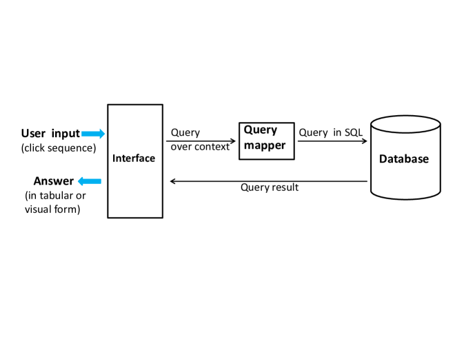
Figure 7: Information flow in the interface

In the interface that we have designed and implemented doi:10.1080/10447318.2022.2073007 , interaction between the user and the interface occurs in four steps as follows:

Step 0: The relational database, call it RDB, is represented as a context, say RDB-Context (as we saw in the introduction) and the interface shows to the user this context (with its nodes clickable).

Step 1: The user clicks on a set of nodes $A_{1}$, …, $A_{n}$ of the RDB-context (meaning that the user requests if there is a relation between these nodes).

Step 2: The system responds by showing to the user $n$ proposals. Each proposal consists of a key node $K$ and a set $P(A_{i})$ of parallel paths with source $K$ and target $A_{i}$, $i=1,\ldots,n$.

Step 3: The user selects one proposal and one path $p_{i}$ from $P(A_{i})$, for each $A_{i}$, $i=1,\ldots,n$ (and eventually defines restrictions on the nodes of the selected paths). This defines the user’s analysis context, call it $\mathcal{C}_{u}$, which is a tree. The user can now ask analytic queries over $\mathcal{C}_{u}$ through a sequence of clicks as will be described shortly.

Step 4: The interface translates each analytic query submitted by the user as an SQL Group-by query $Q$ on the underlying relational database which evaluates $Q$ and returns a relation that the user can visualize as a table and/or in some other visual form.

The information flow in the interface is described succinctly by the diagram of Figure 7.

Additionally, the interface provides a zooming facility when the context graph is very large, so that the user can concentrate on a sub-graph of interest of (conceptually) manageable size, before starting with Step 1.

Note that in Step 1 above the interface provides also an alternative interaction: apart from clicking the nodes $A_{1}$, …, $A_{n}$ the user may also click a node $K$ to be used as the key of the requested relation. In this case all proposals by the system in Step 2 are relations with key $K$. For more details on this interface and user interaction with the system the reader is referred to doi:10.1080/10447318.2022.2073007 .

Note also that once a relation has been extracted the interface can also be used to define usual relational algebra queries. For example, to define a projection of the extracted relation it is sufficient to select the keyword ‘projection’ (from a menu) and then click on the attributes over which projection is to be done; to define a selection it is sufficient to select the keyword ‘selection’ and then click on attributes, one by one, giving the value(s) to be selected for each of the clicked attributes; and so on. For more details the user is referred to doi:10.1080/10447318.2022.2073007 .

To illustrate the interaction between the user and the system consider the data warehouse containing the relations $R,R1,R2,R3,R4$ as defined in the introduction. Setting up the interface requires two preliminary steps: (a) define the RDB-context which, in this case, is the context shown in Figure 1(b) and explained in the introductory section and (b) select the visualization templates to be used. These actions constitute the preliminary Step 0.

After these two actions, the information flow in the interface follows the diagram of Figure 7, where the user’s clicks are translated by a mapper into an SQL Group-by query on the underlying relational database; then the query is evaluated and the result is sent to the interface. As an option, the user can click a desired visualization template from a pop-up menu so as to visualize the result according to the selected template. In order to test the interface, we have experimented with the Pentaho-Mondrian food database (http://mondrian.pentaho.com) as described in detail in doi:10.1080/10447318.2022.2073007 .

To illustrate how an analytic query is defined by the user through a sequence of clicks, consider again the context of Figure 1(b). A user who wants to define the analytic query ‘totals by $Region$’ (formally: $(r\circ b,q,sum)$) will go through the following steps:

Grouping function mode: The user clicks on the nodes $Inv,Branch,Region$ thus defining the path $r\circ b$

Measuring function mode: The user clicks on the nodes $Inv,Qty$ thus defining the path $q$

At this point the interface determines the aggregate operations applicable on $Qty$ and shows to the user a pop-up menu containing these operations; the user clicks one (or more) operations in the menu.

Result visualization mode: The user clicks a visualization template from a pop-up menu (tabular, pie, scatter plot, histogram etc.)

The above actions specify completely the analytic query, as ‘clicked’ by the user, as well as the form in which the user will receive the result.

Summarizing what we have seen in this subsection, we can say that we have demonstrated (a) that the functional algebra allows for the definition of analytic queries in a seamless manner and (b) that a context can be used as an interface to a relational database for data analysis purposes.

4 Concluding remarks and perspectives

In this paper we have seen a data model in which the data sets of an application and their relationships are represented as a labeled, directed, acyclic graph that we called a context. The nodes of a context are the data sets of the application and each edge represents a relation from its source node to its target node. We have also defined the concept of database over a context as an assignment $\delta$ of finite sets of values to the nodes and of finite total functions to the edges.

The nodes and edges of a context can be combined using a set of basic operations on functions that we called the functional algebra of the context; and the set of all well-formed expressions of the functional algebra constitutes the query language of the context. The answer to a query $Q$ with respect to a database $\delta$ is then defined by replacing the nodes and edges appearing in $Q$ by the values assigned to them by $\delta$ and performing the operations.

We have also seen that an analytic query can be defined seamlessly in the functional algebra in contrast to the relational model where analytic queries are defined outside the relational algebra (as group-by queries in SQL).

A prominent feature of our approach is that contexts are treated as ‘first class citizens’ in the sense that we study the concepts of context and database over a context in their own right and then we use the results of our study to gain more insight into some fundamental concepts of relational databases.

To demonstrate the expressive power of our model, we have shown how a consistent relational database can be seen as a view of he context defined by its functional dependencies. We have also demonstrated the applicability of our model by showing how a context can serve as an interface to relational databases for data analysis purposes; and we have designed, implemented and experimented such an interface using the Mondrian food database.

In future work we plan to follow three main lines of related research. First, in view of the embedding of relations as subcontext queries in our model, we would like to revisit fundamental issues of relational database theory such as functional dependency theory, foreign keys, inclusion dependencies, decomposition theory, the chase algorithm and so on, and see how such concepts can be embedded in the context model.

Second, we would like to define update and transaction languages for the context model. Updating in a context $\mathcal{C}$ can happen at two levels: updating the graph $\mathcal{C}$ or updating the database $\delta$. Updating the graph $\mathcal{C}$ means adding or removing edges under the constraint that the graph remains acyclic. In a relational database, this operation corresponds to changing the schema which is extremely complex and costly as it means migrating the data of the database to the new schema (a problem related to data exchange FKMP03 ; FKP05 ). On the other hand, updating the database $\delta$ means changing the function assigned to an edge $f:X\to Y$. This can be done by inserting a pair of values $(x,y)$ not already in $f$ or by deleting or modifying a pair of values $(x,y)$ already in $f$. The constraint that has to be maintained during these operations is that all functions in the updated database $\delta$ must be total functions.

Finally, as an analytic query is a triple of functions and its answer is also a function, we would like to define a ‘visualisation algebra’ for manipulating visualisations of analytic query answers along the lines of SpyratosS19 .

References

- [1] Renzo Angles, Marcelo Arenas, Pablo Barceló, Aidan Hogan, Juan L. Reutter, and Domagoj Vrgoc. Foundations of modern graph query languages. CoRR, abs/1610.06264, 2016.
- [2] Marcelo Arenas, Claudio Gutierrez, and Juan F. Sequeda. Querying in the age of graph databases and knowledge graphs. In Guoliang Li, Zhanhuai Li, Stratos Idreos, and Divesh Srivastava, editors, SIGMOD ’21: International Conference on Management of Data, Virtual Event, China, June 20-25, 2021, pages 2821–2828. ACM, 2021.
- [3] Ronald Fagin, Phokion G. Kolaitis, Renée J. Miller, and Lucian Popa. Data exchange: Semantics and query answering. In Database Theory - ICDT, 9th International Conference, Italy, Proceedings, pages 207–224, 2003.
- [4] Ronald Fagin, Phokion G. Kolaitis, and Lucian Popa. Data exchange: getting to the core. ACM Trans. Database Syst., 30(1):174–210, 2005.
- [5] Claudio Gutierrez, Jan Hidders, and Peter T. Wood. Graph data models. In Sherif Sakr and Albert Y. Zomaya, editors, Encyclopedia of Big Data Technologies. Springer, 2019.
- [6] Aidan Hogan. Knowledge graphs: A guided tour (invited paper). In Camille Bourgaux, Ana Ozaki, and Rafael Peñaloza, editors, International Research School in Artificial Intelligence in Bergen, AIB 2022, June 7-11, 2022, University of Bergen, Norway, volume 99 of OASIcs, pages 1:1–1:21. Schloss Dagstuhl - Leibniz-Zentrum für Informatik, 2022.
- [7] Aidan Hogan, Eva Blomqvist, Michael Cochez, Claudia d’Amato, Gerard de Melo, Claudio Gutierrez, Sabrina Kirrane, José Emilio Labra Gayo, Roberto Navigli, Sebastian Neumaier, Axel-Cyrille Ngonga Ngomo, Axel Polleres, Sabbir M. Rashid, Anisa Rula, Lukas Schmelzeisen, Juan F. Sequeda, Steffen Staab, and Antoine Zimmermann. Knowledge graphs. ACM Comput. Surv., 54(4):71:1–71:37, 2022.
- [8] Maria-Evangelia Papadaki, Nicolas Spyratos, and Yannis Tzitzikas. Towards interactive analytics over RDF graphs. Algorithms, 14(2):34, 2021.
- [9] Jaroslav Pokorný. Graph databases: Their power and limitations. In Khalid Saeed and Wladyslaw Homenda, editors, Computer Information Systems and Industrial Management - 14th IFIP TC 8 International Conference, CISIM 2015, Warsaw, Poland, September 24-26, 2015. Proceedings, volume 9339 of Lecture Notes in Computer Science, pages 58–69. Springer, 2015.
- [10] Nicolas Spyratos. A functional model for data analysis. In Henrik Legind Larsen, Gabriella Pasi, Daniel Ortiz Arroyo, Troels Andreasen, and Henning Christiansen, editors, Flexible Query Answering Systems, 7th International Conference, FQAS 2006, Milan, Italy, June 7-10, 2006, Proceedings, volume 4027 of Lecture Notes in Computer Science, pages 51–64. Springer, 2006.
- [11] Nicolas Spyratos and Tsuyoshi Sugibuchi. HIFUN - a high level functional query language for big data analytics. J. Intell. Inf. Syst., 51(3):529–555, 2018.
- [12] Nicolas Spyratos and Tsuyoshi Sugibuchi. Data exploration in the HIFUN language. In Alfredo Cuzzocrea, Sergio Greco, Henrik Legind Larsen, Domenico Saccà, Troels Andreasen, and Henning Christiansen, editors, Flexible Query Answering Systems - 13th International Conference, FQAS 2019, Amantea, Italy, July 2-5, 2019, Proceedings, volume 11529 of Lecture Notes in Computer Science, pages 176–187. Springer, 2019.
- [13] Jeffrey D. Ullman. Principles of Databases and Knowledge-Base Systems, volume 1-2. Computer Science Press, 1988.
- [14] Katerina Vitsaxaki, Stavroula Ntoa, George Margetis, and Nicolas Spyratos. Interactive visual exploration of big relational datasets. International Journal of Human–Computer Interaction, 0(0):1–15, 2022.
- [15] Gio Wiederhold. Mediation in information systems. ACM Comput. Surv., 27(2):265–267, 1995.
- [16] Petros Zervoudakis, Haridimos Kondylakis, Nicolas Spyratos, and Dimitris Plexousakis. Query rewriting for incremental continuous query evaluation in HIFUN. Algorithms, 14(5):149, 2021.