On the relevance of APIs facing fairwashed audits

Abstract

Recent legislation required AI platforms to provide APIs for regulators to assess their compliance with the law. Research has nevertheless shown that platforms can manipulate their API answers through fairwashing. Facing this threat for reliable auditing, this paper studies the benefits of the joint use of platform scraping and of APIs. In this setup, we elaborate on the use of scraping to detect manipulated answers: since fairwashing only manipulates API answers, exploiting scraps may reveal a manipulation. To abstract the wide range of specific API-scrap situations, we introduce a notion of proxy that captures the consistency an auditor might expect between both data sources. If the regulator has a good proxy of the consistency, then she can easily detect manipulation and even bypass the API to conduct her audit. On the other hand, without a good proxy, relying on the API is necessary, and the auditor cannot defend against fairwashing.

We then simulate practical scenarios in which the auditor may mostly rely on the API to conveniently conduct the audit task, while maintaining her chances to detect a potential manipulation. To highlight the tension between the audit task and the API fairwashing detection task, we identify Pareto-optimal strategies in a practical audit scenario.

We believe this research sets the stage for reliable audits in practical and manipulation-prone setups.

1 Introduction

Regulators are institutions that are typically put in charge by states (see e.g. [11]) to assess the compliance of platforms with the law. To facilitate access to relevant data, a standard approach for regulators is to ask platforms to open up Application Programming Interfaces (APIs) [11, 12] (as YouTube contextual recommendation API [27] or Amazon’s APIs for algorithmic pricing [3]).

Unfortunately, it has been shown that such APIs can be manipulated [23, 1, 2, 18]. Indeed, using the API clearly identifies the auditor to the platform, and the consequences (trial, fine, reputation) of a negative audit outcome provides a clear incentive for malicious platforms to game the audit. The danger of this situation is to have platforms behave compliantly with auditors only, while conserving a non-compliant (but perhaps economically desirable) behavior with all regular users. This setup constitutes a serious threat to the reliability of auditing: focusing on a single data source falls short.

In this paper, we focus on a simple strategy auditors can rely on to mitigate this reliability threat. Despite the wide variety of audit situations, the key element to fairwashing strategies is to behave differently with auditors than with regular users. For an auditor, checking the consistency of a platform’s answers from both a user and an API perspective is hence of interest. Like mystery shoppers, auditors should thus covertly query data as regular users to seek inconsistencies and detect fairwashing.

To query such data, auditors can submit crafted queries from the platform service, or can scale by designing bots that emulate real users and scrape the platform’s website [16, 10]. Unfortunately, scraping is arguably more challenging than using an API. Bots need to be tailored to the specifics of the platform’s web interface. Bots also need to exhibit human-like behavior for evading bot detection mechanisms [17]. In particular, bots are usually bound to limited query rates, which limits the quantity of queried data. Finally, in contrast to APIs purposely designed to provide audit-relevant data, scraping only yields public data that might only be very remotely connected to the audit property [10]. Hence, depending on the specific context, scraping may yield data of insufficient quality or quantity to support the audit.

To sum up, we consider settings where auditors have access to two distinct data sources to audit a potentially malicious platform: i) specifically designed APIs that conveniently provide the right information but are prone to manipulation, and ii) scraping approaches that provide non-manipulated data about the platform behavior but might come in insufficient quantity and/or quality to support the audit. This paper proposes to formalize this setup and study the conditions under which the auditor can nevertheless produce a reliable (i.e. non-fairwashed) audit.

Contributions.

More specifically, and after introducing the API auditing problem in Section 2, we make the following two main contributions: 1) we formalize the notion of consistency (Sections 3 and 4) that binds data queried from both perspectives under the generic form of a (statistical) proxy. We identify three canonical proxies, and study their impact on reliable audits. 2) We experimentally study a query-efficient Pareto-optimal strategy (Section 5) in which the regulator maximizes the quality of the audit and the probability to detect manipulation, by leveraging a two-armed approach on both the API and the scraped data source.

2 The API Auditing Problem

We now define the API auditing problem, illustrated in Figure 1. We consider a threat model where a regulator audits a platform $\mathbf{P}$ through two distinct data sources $\mathbf{A}$ (the API) and $\mathbf{B}$ (scraping), with a budget constraint on the number of queries. She aims to assess if a property holds, using an evaluation function $h_{*}$ applied to $\mathbf{P}$. $\mathbf{P}$ might be manipulative, by modifying the answers of $\mathbf{A}$ to prevent $h_{*}$ to conclude on a violation of the property [1, 2, 18, 23].

2.1 The auditing power of the regulator

In a common audit setup [19], the goal of the regulator is to produce a binary decision, coined $Z$, using a function $h_{*}$ that evaluates a property on a platform $\mathbf{P}$.

We consider that $Z=0$ is an audit outcome that has a negative consequence, e.g. $Z$ is "is $\mathbf{P}$ fair concerning group xyz ?", in which case $Z=0$ implies $\mathbf{P}$ is unfair and liable for prosecution. Formally, $Z=h_{*}(\Omega_{\mathbf{A}})\in\{0,1\}$ with $\Omega_{\mathbf{A}}$ the set of all queries and answers pairs gathered from $\mathbf{A}$.

The regulator constructs an estimator, which is a function from the function space $\mathcal{H}=\{h:S\rightarrow Z\}$ containing functions that can be defined on a dataset $S$ to $\{0;1\}$. We address the audit problem from an empirical risk minimization (ERM) perspective [8, 15].

Figure 1: The ideal auditing scenario uses a trusted audit API $\mathbf{A}$ (that is non-manipulative), leading to an accurate audit (left). (center) We consider a manipulative platform (orange arrows): in the absence of a proxy (red cross), the regulator cannot verify the outcome of $\mathbf{A}$ nor estimate $h_{*}$ with $\mathbf{B}$. (Right) The existence of a good or perfect proxy allows for both checking the consistency of API answers from scraped data and reliably audit $\mathbf{P}$.

The regulator constructs the estimator of $h_{*}$ from $\mathbf{A}$’s answers, using $t$-accuracy:

Definition 1.

$t$-accuracy.
An estimator $\hat{h}_{t}$ is $t$-accurate if and only if, by using $t$ samples, it is a probably approximately correct estimator of $h_{*}$, where $h_{*}$ can be defined such as $h_{*}=\underset{h\in\mathcal{H}}{argmin}\{R(h)\}$ with $R$ the expectation of a loss function $l$. That is to say, $\hat{h}_{t}$ satisfies a concentration inequality of the type:

$$\forall\epsilon,\exists\delta,\mathds{P}(R(\hat{h}_{t})-R(h_{*})\geq\epsilon)\leq\delta,$$ (1)

We shorthand the notation $\hat{h}_{t}$ by $\hat{h}$. The index will instead specify on which samples the estimator works, e.g. $\hat{h}_{\mathbf{A}}$ is a $t_{\mathbf{A}}$-accurate estimator of $h_{*}$ on a dataset from $\mathbf{A}$ of size $t_{\mathbf{A}}$.

From a $t_{\mathbf{A}}$-accurate estimator $\hat{h}_{\mathbf{A}}$, the regulator thus decides on her audit on $\mathbf{P}$ thanks to $\mathbf{A}$.

2.2 Regulator’s access to data

The regulator queries some input $x_{\mathbf{A}}\in\mathcal{X}_{\mathbf{A}}$ from $\mathbf{A}$ and gets label $\mathbf{A}(x_{\mathbf{A}})\in\mathcal{Y}_{\mathbf{A}}$ in return. An audit budget of $t$ means that the regulator can query up to $t$ such queries to decide on an outcome. The samples queried from $\mathbf{A}$ are noted $S_{\mathbf{A}}=(X_{\mathbf{A}},Y_{\mathbf{A}})=\{(x_{\mathbf{A}},\mathbf{A}(x_{\mathbf{A}}),(x^{\prime}_{\mathbf{A}},\mathbf{A}(x^{\prime}_{\mathbf{A}})),\cdots\}\subset\Omega_{\mathbf{A}}$ where $\Omega_{\mathbf{A}}=\mathcal{X}_{\mathbf{A}}\times\mathbf{A}(\mathcal{X}_{\mathbf{A}})$. When the number of samples is relevant, the pairs are noted $S_{\mathbf{A}}^{t_{\mathbf{A}}}$.

Similarly, we define the same sets $S_{\mathbf{B}}$ and universe $\Omega_{\mathbf{B}}$ from the data queried from $\mathbf{B}:\mathcal{X}_{\mathbf{B}}\rightarrow\mathcal{Y}_{\mathbf{B}}$ by replacing $\mathbf{A}$ with $\mathbf{B}$ in the previous notations.

The regulator queries samples from $\mathbf{A}$ and $\mathbf{B}$. The platform can manipulate the answers of $\mathbf{A}$ to appear compliant with the law, without the regulator being able to detect the manipulation (fairwashing). In other words, the answers of $\mathbf{A}$ might be manipulated to cover bias (as shown in [21]), while the actual biased model at the heart of the platform remains unchanged.

3 Formalizing the Relation Between API $\mathbf{A}$ and Scrap $\mathbf{B}$: Consistency

As $\mathbf{A}$ and $\mathbf{B}$ are two sources of information provided by $\mathbf{P}$, a regulator may expect a consistency relation mapping them: a proxy. We model the regulator proxy as a function $\phi:\Omega_{\mathbf{A}}\times\Omega_{\mathbf{B}}\mapsto[0,1]$ such that $\phi(S_{\mathbf{A}},S_{\mathbf{B}})=\mathds{P}(S_{\mathbf{A}}|~S_{\mathbf{B}})$.

As an illustration, consider an API $\mathbf{A}$ simply providing programmer-friendly access to website data $\mathbf{B}$ (as Twitter [24] provides). In such a case, one expects to query the same data from $\mathbf{A}$ and from $\mathbf{B}$, that is $\forall x\in\mathcal{X}_{\mathbf{B}},\mathbf{B}(x)=\mathbf{A}(x)$ with $\mathcal{X}_{\mathbf{A}}=\mathcal{X}_{\mathbf{B}}$ and $\mathcal{Y}_{\mathbf{A}}=\mathcal{Y}_{\mathbf{B}}$. The proxy is the indicator function: $\phi((x,\mathbf{A}(x))|(x,\mathbf{B}(x)))=\mathbbm{1}_{\{\mathbf{A}(x)=\mathbf{B}(x)\}}$.

In a more elaborate example, Dunna et al. [10] use several proxies in their study on YouTube’s demonetization algorithm. Among these, they identify controversial topics on YouTube by using banned or quarantined Subreddit topics queried from Reddit [5]. This proxy could be formally expressed by: $\phi(\text{topic controversial on YT}|\text{topic in Reddit})=\mathds{P}(\text{topic controversial on Reddit})$.

The quality of the proxy at hand is thus crucial: while an identity function does not convey any error, the YouTube example is prone to imprecision; we focus on this aspect in the next section.

The existence of a quality proxy can then be leveraged to detect manipulation. We assume that only the answers of $\mathbf{A}$ can be manipulated. The consistency between $\mathbf{A}$ and $\mathbf{B}$ is captured as follows:

Definition 2.

$\zeta-$Consistency.
Let $\phi$ a proxy, and $S_{\mathbf{B}}\in\Omega_{\mathbf{B}}$ (resp. $S_{\mathbf{A}}\in\Omega_{\mathbf{A}}$) corresponding samples from $\mathbf{B}$ (resp. $\mathbf{A}$). We say that $\mathbf{A}$ is $\zeta$-consistent with $\mathbf{B}$ iff $\phi(S_{\mathbf{A}},S_{\mathbf{B}})\geq\zeta$. When the context is clear, we shorthand the notation and focus on the converse case: $S_{\mathbf{A}}$ and $S_{\mathbf{B}}$ are inconsistent when $\phi(S_{\mathbf{B}},S_{\mathbf{A}})<\zeta$.

As $\phi$ and $\zeta$-consistency are often jointly used we define a set of consistent samples.

Definition 3.

Set of consistent samples.
$\psi$ is a function that associates with each sample $S_{\mathbf{B}}$ the set of consistent samples $S_{\mathbf{A}}$ that would be $\zeta$-consistent for $\phi$: $\forall S_{\mathbf{B}}\in\Omega_{\mathbf{B}},\psi(S_{\mathbf{B}})=\{S_{\mathbf{A}}\in\Omega_{\mathbf{A}}\text{ s.t. }\phi(S_{\mathbf{A}},S_{\mathbf{B}})>\zeta\}$.

Figure 2: Characteristics of the API depending on the proxy quality, and results shown in this paper.

We now expose three canonical proxies:

1) The perfect proxy $\phi^{p}$ is a proxy checking the consistency for all data queried from $\mathbf{A}$: $\forall S_{\mathbf{A}},\exists S_{\mathbf{B}}$ s.t. $\psi^{p}(S_{\mathbf{B}})=\{S_{\mathbf{A}}\}$. As a slight notation abuse, we write $\psi^{p}(S_{\mathbf{B}})=S_{\mathbf{A}}$. With a perfect proxy $\phi^{p}$, samples are inconsistent when the auditor queries $S^{\prime}_{\mathbf{A}}\neq\psi^{p}(S_{\mathbf{B}})$. We stress that such perfect proxies often exist, for instance when $\mathbf{A}$ is simply a programmer-friendly version of $\mathbf{B}$ that provides the exact same data.

2) A poor proxy $\phi^{\emptyset}$ is a proxy that does not perform better than random: $\forall S_{\mathbf{A}},\forall S_{\mathbf{B}},\phi^{\emptyset}(S_{\mathbf{A}},S_{\mathbf{B}})=\frac{1}{|\mathcal{X}_{\mathbf{A}}|}$. As a consequence, assuming $\zeta<\frac{1}{|\mathcal{X}_{\mathbf{A}}|}$, we have $\forall S_{\mathbf{B}},\psi^{\emptyset}(S_{\mathbf{B}})=\mathcal{X}_{\mathbf{A}}\times\mathcal{Y}_{\mathbf{A}}$. $\phi^{\emptyset}$ does not allow detecting any inconsistency.

3) Intermediate proxies: any proxy whose quality lies in between $\phi^{\emptyset}$ and $\phi^{p}$.

Equipped with this proxy quality gradation, we now define two desirable properties on APIs.

Definition 4.

Verifiable.
When the proxy is perfect, we say that $\mathbf{A}$ is verifiable if and only if the regulator can verify each API declaration using $\mathbf{B}$: $\forall S_{\mathbf{A}}\exists S_{\mathbf{B}},~{}s.t.~{}\psi^{p}(S_{\mathbf{B}})=S_{\mathbf{A}}$.

We now define the necessity of an API, i.e. to what extent is it possible to audit a platform without using $\mathbf{A}$?

Definition 5.

API necessity.
The API $\mathbf{A}$ is said necessary if the regulator cannot have an accurate estimator of the property without querying from $\mathbf{A}$. In the opposite case, $\mathbf{A}$ is said not necessary.

Typically, an API could be necessary if it provides information that can neither be queried from $\mathbf{B}$ (because it is not available in the user interface) nor be inferred from scraped data.

Notice that, as the property is evaluated on samples $S$, if the answers have been manipulated, the $t$-accuracy concerns these manipulated pairs $S$ and not the true and unknown samples from $\mathbf{P}$. In the following, we will show that a necessary API cannot be resilient to manipulation.

3.1 With a poor proxy, APIs are necessary

We technically show in Appendix A.1 that a regulator having a poor proxy $\phi^{\emptyset}$ cannot detect manipulation during an audit (i.e. cannot exhibit inconsistency). It can be stated as follows (thm. 3): If the best proxy that the regulator has is the poor proxy $\phi^{\emptyset}$, then there is a strategy for the platform to manipulate $\mathbf{A}$ for compliance with the property. Thus, if $\phi^{\emptyset}$ is the best proxy available to the regulator, then $\mathbf{A}$ is necessary (thm. 4). It means that the regulator cannot estimate $h_{*}$ with $\mathbf{B}$ using $\hat{h}_{\mathbf{A}}$, with the same theoretical guarantees.

3.2 With a perfect proxy, APIs are not necessary

This section exposes the central result of this paper for regulators: it demonstrates that if the API is verifiable, then it is not necessary (because the regulator can estimate $h_{*}$ solely thanks to $\mathbf{B}$).

Theorem 1.

Consider a platform with a verifiable API $\mathbf{A}$ and a proxy $\phi$ with its corresponding $\psi$. A regulator has an estimator $\hat{h}_{\mathbf{A}}$ of a property $h_{*}$ with $t_{\mathbf{A}}$ queries from $\mathbf{A}$. From an ERM perspective, if $\hat{h}_{\mathbf{A}}$ satisfies a concentration inequality (as Equation 1), then for any query’s budget $t_{\mathbf{B}}$ from $\mathbf{B}$ greater than a known budget, the regulator can estimate the property using $\mathbf{B}$ with an estimator $\hat{h}_{\mathbf{B}}$, and this estimator satisfies the same concentration inequality. Which is expressed mathematically as:

$$\begin{matrix}\forall t_{\mathbf{A}}\in\mathbb{N},\exists\psi:S_{\mathbf{B}}\rightarrow S_{\mathbf{A}},\exists~\hat{h}_{\mathbf{A}}:S_{\mathbf{A}}^{t_{\mathbf{A}}}\rightarrow Z,\forall\epsilon,\exists\delta_{\epsilon},\\ \mathds{P}(R(~\hat{h}_{\mathbf{A}})-R(h_{*})\geq\epsilon)\leq\delta_{\epsilon}\end{matrix}\Rightarrow\begin{matrix}\forall t_{\mathbf{B}}\geq sup|\psi^{-1}(S_{\mathbf{A}}^{t_{\mathbf{A}}})|,\exists~\hat{h}_{\mathbf{B}}:S_{\mathbf{B}}^{t_{\mathbf{B}}}\rightarrow Z,\\ \mathds{P}(R(~\hat{h}_{\mathbf{B}})-R(h_{*})\geq\epsilon)\leq\delta\end{matrix}$$

In other words, if a proxy is powerful enough to verify an API, it can also be directly exploited to robustly emulate the API with $\mathbf{B}$: the regulator can estimate the property regardless of any fairwashing.

A more direct claim follows from the contrapositive of theorem 1:

Theorem 2.

If the API $\mathbf{A}$ is necessary then it is not verifiable, i.e. the regulator can only blindly trust the API.

The proofs for both theorems are deferred in Appendix A.2.

3.3 The intermediate case: good enough proxies

The global picture (fig. 1) is the following: the best possible proxy $\phi^{p}$ allows to detect any possible manipulation, and hence ensures a verifiable API. However, this implies (thm. 1) that the same API is not necessary, as it can be directly emulated by the regulator through the same proxy. In the case of a poor proxy $\phi^{\emptyset}$, the API is necessary and cannot be replaced (thm. 4), while in the meantime its answers can be manipulated (thm. 3).

What happens for intermediate proxies that are neither poor, nor perfect, yet good enough? While a complete exploration of those cases goes beyond the scope of this paper, one can observe that: in some cases, a proxy can be sufficiently powerful to emulate $\mathbf{A}$ (thus making $\mathbf{A}$ not necessary), while not being sufficiently powerful to make $\mathbf{A}$ verifiable.

For instance, let $\phi^{i}$ be an intermediate proxy, with the corresponding $\psi^{i}$, that rules out all but one alternative API declaration $\mathbf{A}^{\prime}$:

Observation 1.

If there exists $\psi^{i}$ s.t. $\forall S_{B},\psi^{i}(S_{B})=\{S_{A},S_{A}^{\prime}\}$ and $\hat{h}_{A}(S_{A})=\hat{h}_{A}(S_{A}^{\prime})$, then $\mathbf{A}$ is not necessary.

In such cases, since both $S_{A}$ and $S_{A}^{\prime}$ always both yield the same audit result, $\mathbf{A}$ is not necessary. In other words, here $\mathbf{A}$ is not necessary before being verifiable, hence compromising the equivalence between verifiable and non-necessary.

Another case is possible when the intermediate proxy $\phi^{i}$ miss-maps some samples: $\exists S_{\mathbf{B}},\psi^{i}(S_{\mathbf{B}})\neq\psi^{p}(S_{\mathbf{B}})$. If the number of errors is small compared to the number of pairs, then the intermediate proxy may be sufficient to estimate some violation of the property. A simulation of such a good enough proxy is presented in Appendix B.

We conclude that from a decidability perspective, APIs are not necessary to check compliance when the regulator has a good enough proxy at hand.

4 Experimental Illustrations

In Section 3, we have connected the notions of proxy quality, API necessity, and API verifiability. The following experiments illustrate these, in the case the regulator has a perfect proxy to audit an online video-sharing platform. Both non-manipulated API (sec. 4.1) and manipulated API (sec. 4.2) are explored. Configurations where a regulator has only an intermediate proxy are developed in Appendix B, where we use the Census Income dataset with a trained machine-learning model.

4.1 A perfect proxy, a non-manipulated API

We consider some content creators publishing videos on an online sharing platform. Users are enjoying these videos. The platform compensates content creators for their videos, depending on their popularity and the monetization parameter of each video. A regulator wants to verify if creator’s earnings are indeed proportional to the popularity of the content they publish.

The regulator setup.

The setup is depicted in Figure 6 in the Appendix. The regulator has access to two data sources: $\mathbf{A}$ is an API that returns the popularity $p$ and the earnings $e$ of each content creator $c$, while $\mathbf{B}$ is the website interface for viewing videos: the regulator gets for each video $v$: its number of views $m$, and its monetization rate $r$ defined as the amount of money per view gained by its creator $c$. We thus have $\mathbf{A}:c\mapsto p,e$ and $\mathbf{B}:v\mapsto m,r,c$.

The regulator uses the following proxy $\psi$ for her audit: $\psi:(v,m,r,c)\mapsto(c,p,e)$.

As in [10], the popularity $p$ is estimable as the sum of views on all the videos of a content creator $c$. The earnings of each creator are the sum of views per video weighted by their monetization rate ($e=\sum_{v\in V_{c}}m.r$). This proxy is deemed perfect, as the regulator made a correct guess on the relation between data from $\mathbf{B}$ and $\mathbf{A}$: it allows for a correct assessment of a potential bias.

The property tested by the regulator is the economic parity: "Does the platform compensate creators proportionally to the popularity of the videos they publish?".

Simulation setup.

This simulation leverages the usual $80\%$ ceil for the disparate impact [13]. We can then define economic parity as:

$$h_{*}(\cdots,(c,p,e),(c^{\prime},p^{\prime},e^{\prime}),\cdots)=\left(\mathds{P}\left(e<e^{\prime}|p<p^{\prime}\right)>0.8\right).$$

A platform is violating the property if the monetization rate is not the same for all content creators. To introduce such a bias in our simulation, we set a randomly selected third of the content creators to have a monetization rate $r_{1}=\$0.1$ per view, while the remaining two-thirds a rate $r_{0}=\$0.01$ per view. Creators with a monetization rate $r_{1}$ are called privileged creators.

Simulation results.

We show that if the API is verifiable, then it is not necessary to decide.

The simulation runs $1,000$ content creators, each having published a number of videos following an exponential law. We measure $\mathds{P}\left(e<e^{\prime}|p<p^{\prime}\right)=0.776$. As it is below $0,8$, economic parity is violated ($Z=0$). Under no budget limitation, $h_{*}$ can be estimated with all the samples queried from $\mathbf{A}$ by using a statistical estimator $\hat{h}_{\mathbf{A}}$. We measure $\hat{h}_{\mathbf{A}}(\Omega_{\mathbf{A}})=0.776$.

As $\phi$ and $\psi$ are perfect and the API is not manipulated, we define $\hat{h}_{\mathbf{B}}=~\hat{h}_{\mathbf{A}}\circ\psi$ (with $\circ$ the composition operator). By definition, it is an unbiased estimator of $h_{*}$, assuming that the query budget is large enough to reconstruct all antecedents of entries of $\hat{h}_{\mathbf{A}}$ by $\psi$. That is to say, for all content creators queried on $\mathbf{A}$, the regulator must query all their videos from $\mathbf{B}$ to avoid using $\mathbf{A}$. We measured $\hat{h}_{\mathbf{B}}(\Omega_{\mathbf{B}})=~(\hat{h}_{\mathbf{A}}\circ\psi)(\Omega_{\mathbf{B}})=0.776$ which is the expected result.

Since the $\hat{h}_{\mathbf{B}}$ resulting from the audit is an accurate estimator of the property, it trivially follows that $\mathbf{A}$ is not necessary. This scenario is nevertheless ideal; we now move on to a more elaborate and manipulated case.

4.2 A perfect proxy, a manipulated API

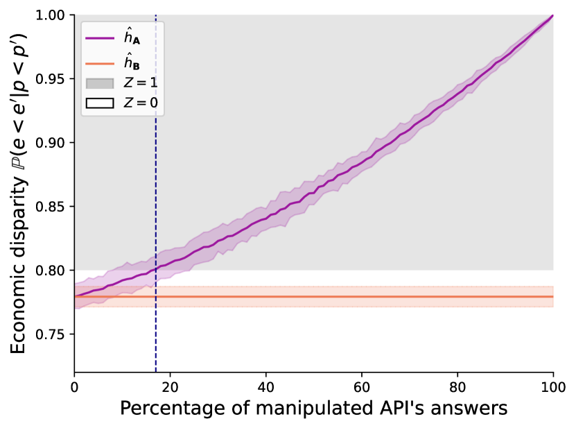
(a) Decreasing privileged creator’s earnings.

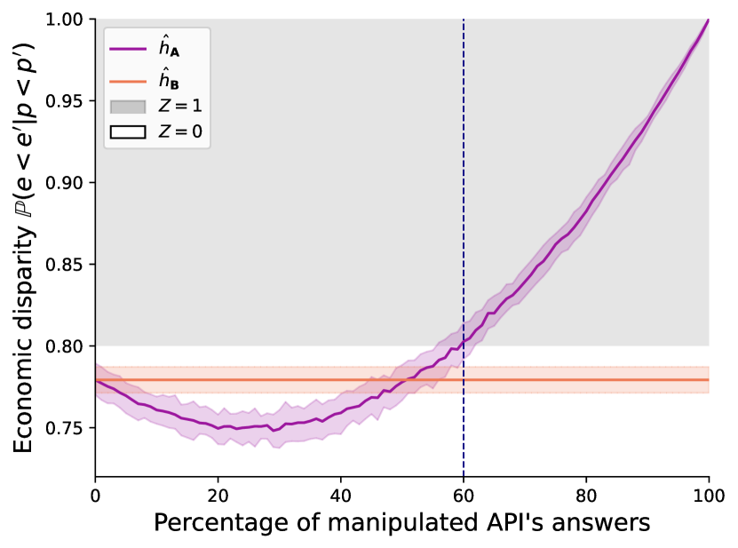
(b) Increasing non-privileged creator’s earnings.

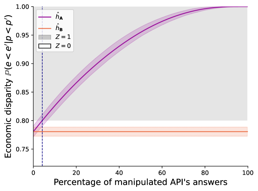
(c) Swapping creator’s earnings

Figure 3: Three strategies for API manipulations by the platform. The $x$-axis on a figure amounts to the percentage of manipulated answers in $\mathbf{A}$, ranging from $0$ to $100\%$. The $y$-axis represents the empirical probability of economic parity. If the probability is greater than $0.8$ (gray zone, $Z=1$), the regulator concludes in compliance with the property. The pink curve (resp. orange) is the evaluation of the estimator of $h_{*}$ using all samples queried from $\mathbf{A}$ (resp. $\mathbf{B}$). The threshold (vertical blue line) is the minimal amount of manipulation on $\mathbf{A}$’s answers to game the audit and prevent concluding on the violation of economic parity. Uncertainties are given for the quantiles ($0.1$ and $0.9$ on $50$ runs).

We now simulate a scenario where the platform is manipulative, in an attempt to cover non-compliance to economic parity (i.e. by trying to hide the existence of privileged creators). The following three manipulation strategies are leveraged by the platform.

Decreasing privileged creator’s earnings.

It is a scenario close to the demonetization observed on some real platforms. The platform manipulates $\mathbf{A}$ by announcing a decrease in the earnings of privileged creators in its answers (considering a monetization rate of $r_{0}$ while their monetization rate must be $r_{1}$) on $x\%$ of the privileged creators on Figure 3(a).

Increasing non-privileged creator’s earnings.

This manipulation (Figure 3(b)) is the opposite of the previous one: the platform manipulates $\mathbf{A}$ to announce an increase in the earnings of non-privileged creators.

Swapping creator’s earnings.

We considered the following list of earnings: the earning in position $i$ is the earning of the creator $i$ where creators are sorted according to their popularity. The economic parity is perfect when this list is sorted. Thus, the platform manipulates $\mathbf{A}$ by sorting the list of earnings following the bubble sort. That is to say, the platform repeatedly compares each element of the list of earnings with the one after it, swapping their values if needed. Those passes through the list are repeated on Figure 3(c) until no swaps had to be performed during a pass, meaning that the list has become fully sorted from $x=0\%$ for no pass, to $x=100\%$ when the list of earnings is sorted.

Results.

Audits for economic parity are depicted in Figure 3. The regulator uses the same $\psi$ as in Section 4.1, as she ignores that the data of $\mathbf{A}$ is being manipulated. For instance, in Figure 3(a), if $x=20\%$ of the privileged creators have their monetization rate manipulated to $r_{0}$, the estimation of the property using $\mathbf{A}$ is $Z=1$ because the economic parity on $\mathbf{A}$ will be greater than $0.8$ (gray area). As only $\mathbf{A}$ is manipulated, the estimation using $\mathbf{B}$ and the proxy (orange curve) is constant.

When the platform manipulates $\mathbf{A}$ to a maximum of $27\%$, it can either improve its equity (cases (a) and (c)) or deteriorate it (case (b)) depending on its manipulation strategy. Cases (a) and (b) are symmetrical: the proportion between privileged and non-privileged must tend to $0$ or $1$ to ensure fairness. To be fair, every creator must be either privileged or not. The worst case is $0.5$, where there are as many privileged as non-privileged creators: it is reached at the minimum of the pink curve in (b). $\hat{h}_{\mathbf{A}}$ is strictly increasing in (c) because sorting swaps reorder the earnings at each step.

With the increasing manipulation of $\mathbf{A}$, there is always a threshold where the manipulation makes the regulator erroneously conclude the compliance with the economic parity while using the manipulated $\mathbf{A}$.

In conclusion, we saw that the platform can manipulate the answers of $\mathbf{A}$ to fool a regulator auditing through $\mathbf{A}$. This illustrates the possibility of fairwashing in practice [1]. Auditing $\mathbf{A}$ thus fools the regulator, while $\mathbf{B}$ is sufficient for an accurate audit; $\mathbf{A}$ is not necessary for this decision task.

5 Query Budget Arbitration: the Choice Between Two Arms

We now analyze a setting where with a budget of $t$ queries, our regulator has two distinct objectives: $i)$ estimating the property of interest $Z$ as accurately as possible and $ii)$ verifying the consistency between $\mathbf{A}$ and $\mathbf{B}$ to detect a manipulative platform. This section deals with the case where the total budget $t$ of the regulator is greater than $t_{\mathbf{A}}$ and when $t_{\mathbf{A}}$ can be mathematically determined depending on the accepted error in the ERM (Equation 1). Please refer to Appendix D.2 for additional strategies in the remaining cases.

The query budget arbitration is modeled by a two-armed problem: the first arm is sending one input to $\mathbf{A}$ for later estimating $\hat{h}_{\mathbf{A}}$, while the second arm is sending one input to $\mathbf{A}$ and several queries to $\mathbf{B}$ to check the consistency of $\mathbf{P}$. With the second arm, for one input $x_{\mathbf{A}}$ the regulator must query $\psi^{-1}(x_{\mathbf{A}})$ from $\mathbf{B}$, which can be very expensive. However, the samples queried from $\mathbf{A}$ by querying $x_{\mathbf{A}}$ can also be later used for estimating $\hat{h}_{\mathbf{A}}$.

The regulator has to find the right trade-off to spend on each arm. Appendix D.1 contains the theoretical analysis for calculating the accuracy of the estimator based on a given budget allocation.

Simulation setup.

We reuse the video platform scenario, where a third of the content creators have a better monetization rate ($r_{1}$) than the others ($r_{0}$). To cover the violation of the economic parity, the platform manipulates $\mathbf{A}$ decreasing the monetization rate of $20\%$ of the privileged creators. We set the regulator’s query’s budget $t$ to $0.25\%$ of the total input space of the platform; this corresponds to around $200$ queries in our setting.

The regulator can distribute her budget as she wishes, in particular by using $t\beta$ queries on the first arm and $t(1-\beta)$ queries on the second arm (with $\beta\in[0,1]$). The probability to detect inconsistencies is evaluated by estimation, while $\epsilon$ is calculated thanks to equation 2.

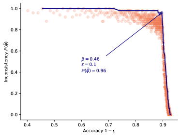
Figure 4: A Pareto frontier in estimating economic parity while also checking for manipulation (inconsistencies between answers from $\mathbf{A}$ and $\mathbf{B}$) under a fixed audit query-budget. Each point of the figure corresponds to a setting for $\beta$.

Results.

Figure 4 presents the empirical probability $\mathds{P}(\bar{\phi})$ that the regulator finds at least one inconsistency as a function of the theoretical error $\epsilon$ of her estimator $\hat{h}_{\mathbf{A}}$. The blue line represents the Pareto frontier, i.e. the set of efficient solutions regarding the trade-off between $\mathds{P}(\bar{\phi})$ and $\epsilon$. That is to say, to efficiently choose her budget, the regulator must choose one point on the blue line. For example, for the margin error $\epsilon=10\%$ (blue point pointed by the arrow), and for a selected $\beta=0.46$, the empirical probability to detect an inconsistency is very high at $\mathds{P}(\bar{\phi})=0.96$.

Under a limited budget to query from the platform, a regulator can then arbitrate her budget to $i)$ accurately perform her audit and to $i)$ detect manipulation on the API.

6 Related Work

Yan and Zhang [26] elaborated on the design of another type of manipulation-proof audit. They target manipulations of the model post-audit, i.e. they aim at preventing that the model is manipulated after an audit while staying consistent with the answers that were given during this initial audit. In that light, they provide an algorithm that guarantees that the platform cannot manipulate a new audit without being detected, thanks to a set of queries that constrain the platform the most. We note that in this work, authors do not consider direct manipulation of the platform answers, as yet shown possible by fairwashing [23, 1, 2, 18], making this work still prone to it.

The result "only non-verifiable APIs are necessary" is a sort of impossibility result that fits well into the current state of the art. For example, the survey [6] enumerates almost fifty impossibility theorems related to problems in the field of AI.

In the audit scenario, fairwashing detection was also studied [23]. In a slightly different setup, the authors also consider two models: a black-box model (corresponding to $\mathbf{B}$ in our model) from which is derived a potentially fairwashed interpretable surrogate model (that would correspond to $\mathbf{A}$ in our model). They then show in this context that a fairwashed demographic parity can be detected by comparing the accuracy of the surrogate for each demographic class. In contrast, our results provide a more general perspective (any property, any relation between $\mathbf{A}$ and $\mathbf{B}$, limited queries to $\mathbf{A}$) and highlights the intrinsic tension of any such model : necessary APIs are non-verifiable. Besides, we provide a construction for a regulator to turn a good enough proxy into an emulator of the API.

7 Limitations

The limitations of our work are as follows:
1) We assume scraping (through $\mathbf{B}$) yields non-manipulated data. This assumption might fail in some contexts, but is unfortunately essential as otherwise the auditor has no chance to produce a reliable audit if she only sees manipulated data, without additional work assumptions.
2) The act of scraping by itself might not qualify as legal evidence, as exemplified since June 2021 by the Computer Fraud and Abuse Act [25], which specifies that regulators can not prove a violation of the CFAA by mere scraping. While in our approach scraping would serve to control consistency, we believe the legal consequences of this approach with respect to specific national regulatory authorities should be assessed by an expert.
3) Besides the extreme (poor and perfect) proxies, the intermediate case covers a wide and diverse variety of situations. We sketched several good enough proxies in this work but did not consider a complete study of this proxy class, that we believe is to be examined on a per-concrete audit basis.

8 Conclusion

Facing the possibility of audit gaming by the platforms, it is critical that the regulators know what are nevertheless the conditions to perform accurate audits. In this paper, we have exposed the benefits of the junction of a second data source to an API to detect audit manipulation.

For building our first contribution that formalizes the notion of proxy consistency, i) we demonstrated in Section 3 that a perfect proxy is desirable, as it enables detecting manipulation and helps performing the audit accurately. Experiments also show that good enough proxies may help in specific cases. We then have proven ii) (sec. 3) that verifiable APIs are not necessary. Interestingly, there is however no strict equivalence between necessity and non-verifiability, and this is observed in cases where APIs are not verifiable and yet not necessary.

In our second contribution, we studied a trade-off (sec. 5) that drives the budget that a regulator may use to perform her audit, while also attempting to detect API manipulation, under a two-armed posed problem.

Altogether, this paper challenges future works to provide ways to derive good proxies, given samples publicly available versus the information that can be extracted from platforms APIs.

Appendix A Proofs for the necessity theorems

A.1 With poor proxies, APIs are necessary

We here provide the proof that if $\phi^{\emptyset}$ is the best proxy available to the regulator, then $\mathbf{A}$ is necessary (stated in Section 3.1). First, we demonstrate the following theorem:

Theorem 3.

If the best proxy that the regulator has is the poor proxy $\phi^{\emptyset}$, then there is a strategy for the platform to manipulate $\mathbf{A}$ for compliance with the property ($Z=1$).

Proof.

The platform knows the queries $X_{\mathbf{A}}$ and the function $h_{*}$ that the regulator estimates. If $\mathbf{A}$ is already in compliance with the propriety ($h_{*}(X_{\mathbf{A}},\mathbf{A}(X_{\mathbf{A}}))=1$) then the platform provides the non-manipulated $\mathbf{A}$ to the regulator. If the property is violated ($h_{*}(X_{\mathbf{A}},\mathbf{A}(X_{\mathbf{A}}))=0$), the platform must find another API $\mathbf{A}^{\prime}$ to be in compliance with the property.

First, assume no such $\mathbf{A}^{\prime}$ exists: it means that there exists a query sequence $X_{\mathbf{A}}$ for which any possible answer leads to a violation of the property. In other words, all platforms are guilty given the input $X_{\mathbf{A}}$, and the audit is trivial.

Second, consider that the platform finds a $\mathbf{A}^{\prime}$ in compliance with the property ($h_{*}(X_{\mathbf{A}},\mathbf{A^{\prime}}(X_{\mathbf{A}}))=1$). As on the regulator side, $\hat{h}_{\mathbf{A}}$ is an accurate estimator of $h_{*}$, then the answer is not violating the property anymore ($\hat{h}_{\mathbf{A}}(X_{\mathbf{A}},\mathbf{A^{\prime}}(X_{\mathbf{A}}))=1$).

Third, since it does not exist a set $S_{\mathbf{B}}$ s.t. $\phi(S_{\mathbf{B}},(X_{\mathbf{A}},\mathbf{A^{\prime}}(X_{\mathbf{A}})))<\zeta$, necessarily $\mathbf{A}^{\prime}$ is consistent with any possible sample queried by the regulator on the $\mathbf{B}$ side. ∎

The regulator cannot use $\mathbf{A}$ without risking being gamed by the platform: the evaluation of the property on $\mathbf{A}$ does not reflect the behavior of the platform. However, as Theorem 4 shows, if the regulator wants to estimate $h_{*}$, she must use $\mathbf{A}$.

Theorem 4.

Fix $\mathbf{A}$ and $\mathbf{B}$, and assume $\phi^{\emptyset}$ is the best available proxy. Then $\mathbf{A}$ is necessary.

Proof.

We proceed by contradiction. Assume $\mathbf{A}$ is useless: then $\exists\hat{h}_{\mathbf{B}}$ s.t. $\hat{h}_{\mathbf{B}}$ is a $t$-accurate estimator of the evaluation function $h_{*}$. Let $Z\in\{0,1\}$ be the property of interest. Observe that $\hat{h}_{\mathbf{B}}$ induces a partition of $\Omega_{\mathbf{B}}$ given its answer: let $\Omega_{\mathbf{B}}^{Z}=\{S_{\mathbf{B}}\in\Omega_{\mathbf{B}}$ s.t. $\hat{h}_{\mathbf{B}}(S_{\mathbf{B}})=Z\}$. Let $\hat{h}_{\mathbf{A}}$ be a $t$-accurate estimator of $h_{*}$ using $\mathbf{A}$’s input. Observe that $\hat{h}_{\mathbf{A}}$ induces a partition of $\Omega_{\mathbf{A}}$ given its answer: let $\Omega_{\mathbf{A}}^{Z}=\{S_{\mathbf{A}}\in\Omega_{\mathbf{A}}$ s.t. $\hat{h}_{\mathbf{A}}(S_{\mathbf{A}})=Z\}$.

The central observation here is that since $\mathbf{A}$ and $\mathbf{B}$ are supposed to both consistently represent $\mathbf{P}$’s properties, estimate property $Z$ both through $\mathbf{A}$ and $\mathbf{B}$ should also be consistent.

Let us define the proxy $\phi_{\hat{h}_{\mathbf{B}}}(S_{\mathbf{A}},S_{\mathbf{B}})=\mathds{P}(\hat{h}_{\mathbf{A}}(S_{\mathbf{A}})=\hat{h}_{\mathbf{B}}(S_{\mathbf{B}}))$. Then, $\forall(S_{\mathbf{A}},S_{\mathbf{B}})\in\Omega_{\mathbf{A}}^{Z}\times\Omega_{\mathbf{B}}^{Z},\mathds{P}(\hat{h}_{\mathbf{A}}(S_{\mathbf{A}})=\hat{h}_{\mathbf{B}}(S_{\mathbf{B}}))=1$ as by definition of $\Omega_{\mathbf{A}}^{Z}$ and $\Omega_{\mathbf{B}}^{Z}$, $\hat{h}_{\mathbf{A}}(S_{\mathbf{A}})=\hat{h}_{\mathbf{B}}(S_{\mathbf{B}})$ in those sets. We set for all others sets, $\forall(S_{\mathbf{A}},S_{\mathbf{B}})\notin\Omega_{\mathbf{A}}^{Z}\times\Omega_{\mathbf{B}}^{Z},\phi_{\hat{h}_{\mathbf{B}}}(S_{\mathbf{A}},S_{\mathbf{B}})=\phi^{\emptyset}(S_{\mathbf{A}},S_{\mathbf{B}})$.
That is to say, $\phi_{\hat{h}_{\mathbf{B}}}$ is better than $\phi^{\emptyset}$ on $\Omega_{\mathbf{A}}^{Z}\times\Omega_{\mathbf{B}}^{Z}$, equal on the rest which contradicts the hypothesis that $\phi^{\emptyset}$ is the best available proxy. ∎

Theorem 3 shows that a regulator having a poor proxy cannot detect manipulations in $\mathbf{A}$ while according to Theorem 4 $\mathbf{A}$ is necessary. In conclusion, for a manipulation-proof audit, the regulator must find a better proxy than $\phi^{\emptyset}$ to verify the compliance of $\mathbf{P}$ with the property $Z$.

A.2 With perfect proxies, APIs are not necessary

Probability distributions $\mathds{P}((X_{\mathbf{A}},Y_{\mathbf{A}})=S_{\mathbf{A}})$ (also noted $\mathds{P}(S_{\mathbf{A}})$) are defined to determine how likely it is to query $S_{\mathbf{A}}$ from $\mathbf{A}$. $\mathds{P}((X_{\mathbf{B}},Y_{\mathbf{B}})=S_{\mathbf{B}})$ (resp. $\mathds{P}(S_{\mathbf{B}})$) is defined likewise on $\mathbf{B}$.

In the case where there is no API manipulation and $\phi$ is perfect. We recall theorem 1:

See 1 This theorem is proved as follows :

Proof.

Even if it means doing a discretization trick as in [14] (defined in Remark 4.1 in [22]), we assume that we are dealing with finite sets and that the expectations defined later are written as discrete sums.

We restrict $\Omega_{\mathbf{A}}=(\mathcal{X}_{\mathbf{A}},\mathcal{Y}_{\mathbf{A}})^{t_{\mathbf{A}}}$ as the universe of all $t_{\mathbf{A}}$ pairs of elements in $(\mathcal{X}_{\mathbf{A}},\mathcal{Y}_{\mathbf{A}})$.

By definition of the risk,

$$R(~\hat{h}_{\mathbf{A}})=\mathbb{E}(l(((X_{\mathbf{A}},Y_{\mathbf{A}}),Z),~\hat{h}_{\mathbf{A}}))$$

By transfer theorem:

$$R(~\hat{h}_{\mathbf{A}})=\sum_{\mathclap{\begin{subarray}{c}S_{\mathbf{A}}\in\Omega_{\mathbf{A}}\\ z\in Z\end{subarray}}}l((S_{\mathbf{A}},z),~\hat{h}_{\mathbf{A}})\mathds{P}((X_{\mathbf{A}},Y_{\mathbf{A}})=S_{\mathbf{A}},Z=z)$$

With the short notations:

$$R(~\hat{h}_{\mathbf{A}})=\sum_{\mathclap{\begin{subarray}{c}S_{\mathbf{A}}\in\Omega_{\mathbf{A}}\\ z\in Z\end{subarray}}}l((S_{\mathbf{A}},z),~\hat{h}_{\mathbf{A}})\mathds{P}(S_{\mathbf{A}},z)$$

Thanks to the equality in the sense of events (only true without data manipulation),

$$\{S_{\mathbf{A}}\}=\bigcup_{\mathclap{S_{\mathbf{B}}\in\psi^{-1}(S_{\mathbf{A}})}}\{S_{\mathbf{B}}\}$$

So:

$$R(~\hat{h}_{\mathbf{A}})=\sum_{\mathclap{\begin{subarray}{c}S_{\mathbf{A}}\in\Omega_{\mathbf{A}}\\ z\in Z\end{subarray}}}l((S_{\mathbf{A}},z),~\hat{h}_{\mathbf{A}})\mathds{P}(\bigcup_{\mathclap{S_{\mathbf{B}}\in\psi^{-1}(S_{\mathbf{A}})}}\{S_{\mathbf{B}}\},z)$$

By distributivity of the conjunction over the disjunction:

$$R(~\hat{h}_{\mathbf{A}})=\sum_{\mathclap{\begin{subarray}{c}S_{\mathbf{A}}\in\Omega_{\mathbf{A}}\\ z\in Z\end{subarray}}}l((S_{\mathbf{A}},z),~\hat{h}_{\mathbf{A}})\mathds{P}(\bigcup_{\mathclap{S_{\mathbf{B}}\in\psi^{-1}(S_{\mathbf{A}})}}\{S_{\mathbf{B}},z\})$$

The events are all 2 to 2 disjoint:

$$R(~\hat{h}_{\mathbf{A}})=\sum_{\mathclap{\begin{subarray}{c}S_{\mathbf{A}}\in\Omega_{\mathbf{A}}\\ z\in Z\end{subarray}}}l((S_{\mathbf{A}},z),~\hat{h}_{\mathbf{A}})\sum_{\mathclap{\begin{subarray}{c}S_{\mathbf{B}}\in\psi^{-1}(S_{\mathbf{A}})\end{subarray}}}\mathds{P}(S_{\mathbf{B}},z)$$

$$R(~\hat{h}_{\mathbf{A}})=\sum_{{\begin{subarray}{c}S_{\mathbf{A}}\in\Omega_{\mathbf{A}}\\ z\in Z\end{subarray}}}\sum_{S_{\mathbf{B}}\in\psi^{-1}(S_{\mathbf{A}})}l((S_{\mathbf{A}},z),~\hat{h}_{\mathbf{A}})\mathds{P}(S_{\mathbf{B}},z)$$

$$R(~\hat{h}_{\mathbf{A}})=\sum_{{\begin{subarray}{c}S_{\mathbf{A}}\in\Omega_{\mathbf{A}}\\ z\in Z\end{subarray}}}\sum_{S_{\mathbf{B}}\in\psi^{-1}(S_{\mathbf{A}})}l((\psi(S_{\mathbf{B}}),z),~\hat{h}_{\mathbf{A}})\mathds{P}(S_{\mathbf{B}},z)$$

By definition of $\psi$ (without data manipulation):

$$R(~\hat{h}_{\mathbf{A}})=\sum_{{\begin{subarray}{c}S_{\mathbf{A}}\in\Omega_{\mathbf{A}}\\ z\in Z\end{subarray}}}\sum_{S_{\mathbf{B}}\in\psi^{-1}(S_{\mathbf{A}})}l((S_{\mathbf{B}},z),~\hat{h}_{\mathbf{A}}\circ\psi)\mathds{P}(S_{\mathbf{B}},z)$$

As $\psi$ is perfect, the probability of any set of pairs of elements $S$ in $(\mathcal{X}_{\mathbf{B}},\mathcal{Y}_{\mathbf{B}})$ is null if $S\notin\Omega_{\mathbf{B}}$ (where $\Omega_{\mathbf{B}}=\mathcal{X}_{\mathbf{B}}\times\mathbf{B}(\mathcal{X}_{\mathbf{B}})$ as defined in the core of the paper).

The number of elements in $\Omega_{\mathbf{B}}$ with non-null probability to success is equal to $t_{\mathbf{B}}=\underset{S^{t_{\mathbf{A}}}_{\mathbf{A}}}{sup}|\psi^{-1}(S_{\mathbf{A}}^{t_{\mathbf{A}}})|$.

We change the partition:

$$R(~\hat{h}_{\mathbf{A}})=\sum_{\mathclap{\begin{subarray}{c}S_{\mathbf{B}}\in\Omega_{\mathbf{B}}\\ z\in Z\end{subarray}}}l((S_{\mathbf{B}},z),~\hat{h}_{\mathbf{A}}\circ\psi)\mathds{P}(S_{\mathbf{B}},z)$$

By definition of the risk:

$$R(~\hat{h}_{\mathbf{A}})=R(~\hat{h}_{\mathbf{A}}\circ\psi)$$

This was to be demonstrated. ∎

Intuitively, to detect a manipulated API, the proxy allows emulating an honest API. If such honest emulation exists, it incidentally implies that the final goal of $\mathbf{A}$ (estimating $h_{*}$) can also be fulfilled by the emulation. As a consequence, $\mathbf{A}$ is not necessary. A more direct claim follows:

We recall theorem 2: See 2

Proof.

Proof by contrapositive of the Theorem 1. ∎

Appendix B Further experiments: A good proxy, a non-manipulated API

In Section 4, we have experimented on a simulated video-sharing platform. The regulator has a perfect proxy between $\mathbf{A}$ and $\mathbf{B}$ and she is facing both a non-manipulated API (sec. 4.1) or a manipulated one (sec. 4.2). We now experiment with a prediction task using a real dataset: the regulator has an intermediate proxy because no perfect proxy exists in this scenario.

Figure 5: Auditing the disparate impact of sex on the prediction of high revenues using logistic regression. Data were taken from [9]. The proxy between $\mathbf{A}$ and $\mathbf{B}$ estimates sex considering first names.

We first describe the data and features of the model used by the platform; a visual representation is given in Figure 5.

B.1 Experiment data

Data is adapted from the "Census Income" dataset available in the UCI Machine Learning repository [9]. It contains $48,842$ instances ($16,281$ instances in the training set, $32,561$ in the test set). According to the demonstration of [4], we retained only six characteristics out of the fourteen of the AdultDataset to focus on the impact of the sex of the profiles:

$W=$

• ’age’

• ’education-num’

• ’capital-gain’

• ’capital-loss’

• ’hours-per-week’

All original features except sex will be denoted $W$ in the sequel. In addition to these characteristics, we added random first names to all profiles among the top $25$ given names in Pennsylvania in $1990$ for each sex and reported in the Table II [4]. Barry et al. show that the last spelled letter of these first names often indicates the sex of the individual. That is, first names are a good estimation to sex. We then consider:

$$g:n\mapsto s,$$

that returns an estimation of the sex $s$ from a name $n$ and the frequencies reported in Table I of [4]. On the test dataset, $g$ predicts the true sex in $69.1\%$ of cases. As not perfect, we qualify it as a good proxy, and we are interested in studying the impact of this imperfection on the audit outcome.

B.2 Evaluation metric

To evaluate the fairness of a model that creates a dataset $S$ containing a protected attribute, we use the disparate impact [13, 7]:

Definition 6.

Disparate impact, the "80% rule".

Given a dataset $S=(X,Y)$ containing a protected attribute (e.g. gender, race, religion…) to classify individuals into a protected group $\mathcal{C}$ from the rest of the population $\mathcal{X}\backslash\mathcal{C}$, we will say that $S$ has disparate impact if

$$Z:=\left(DI=\frac{\mathds{P}(Y=1|X\notin\mathcal{C})}{\mathds{P}(Y=1|X\in\mathcal{C})}\leq 0.8\right)$$

where $\mathds{P}(Y=y|X\in\mathcal{C})$ denotes the conditional probability (evaluated over $S$) that the class outcome is $y$ knowing that the individual is in the protected group.

In the following experiments, we audit the entire test set to compute the disparate impact.

B.3 Experimental setup

The task to be performed by the platform is, given an input profile $X$, to predict whether $X$’s income exceeds $\$50$K/yr ($Y=1$) or not ($Y=0$). This scenario is typically performed by a bank that seeks to predict which customer it will allocate loans to. The platform trains a logistic regression, noted f, on the original data. The data sources of the platform are:

$$\mathbf{A}:W,s\underset{f}{\mapsto}Y$$

$$\mathbf{B}:W,n\underset{g}{\mapsto}W,s^{\prime}\underset{f}{\mapsto}Y,$$

where $s$ is the true sex of individuals, whereas $s^{\prime}=g(n)$ is the predicted sex from first name. Both the API $\mathbf{A}$ and platform user service $\mathbf{B}$ use the logistic regression f to predict $Y$ using $W$. However, the last feature of the input is not the same. $\mathbf{A}$ is using the true sex of individuals, given directly by their profiles, an input of $\mathbf{A}$. $\mathbf{B}$ does not provide this information. The regulator instead relies on an estimation based on names, which are available to her. The corresponding $\psi$ of the proxy between samples queried from $\mathbf{A}$ and from $\mathbf{B}$ is

$$\psi:(W,n,Y)\mapsto(W,g(n),Y).$$

B.4 Results

	DI	$\epsilon$(DI)	Z	$\epsilon$(sex)
$\mathbf{A}$	$0.252$	-	$0$	-
$\mathbf{B}+g$	$0.360$	$43\%$	$0$	$30.9\%$

Table 1: Estimated disparate impact (DI) and its estimation error ($\epsilon$(DI)) on the platform, by using $\mathbf{A}$ or $\mathbf{B}$ with an unlimited budget. $Z=0$ means that the property $h_{*}$ is violated by the algorithm. $\epsilon$(sex) is the error on the estimation of the sex of people with the function $g$ considering names.

As displayed in Table 1, the disparate impact computed using sex on a non-manipulated $\mathbf{A}$ is $0.252$, which is significantly smaller than $0.8$. This means that the API is highly unfair ($Z=0$) with regard to the sex, and that the regulator has a chance to detect it using $\mathbf{A}$. However, if the regulator wants to prove this unfairness only using $\mathbf{B}$, she will leverage $\psi$. The proxy is accurate enough to prove the unfairness of $\mathbf{B}$, without using $\mathbf{A}$, with a classic statistical test, easily computed on the queried samples: $0.360$ is way below $0.8$. This means that the joint use of $\mathbf{B}$ and $\psi$ is sufficient to estimate the violation of the property ($Z=0$), even though her proxy is not perfect. The proxy has $30.9$% errors on the test dataset.

This is another illustration that $\mathbf{A}$ is not necessary to the regulator equipped with an accurate enough proxy.

Appendix C Data for Reproducibility

The code is open-sourced anonymously at: https://pastebin.com/BbThmpGv, and will be open sourced under the GPLv3 licence shall the paper be accepted.

Figure 6: Auditing economic parity on a video sharing platform. The API provides popularity and earnings of content creators, whereas the user interface provides videos and information about videos. The proxy estimates the earnings of creators based on their videos.

Here are the details of the experiments carried out in Sections 4.1,4.2 and 5. The online sharing platform is created for $1000$ content creators. Each content creator has published between $1$ and $100$ videos. The distribution of the number of videos by creators follows an exponential law with parameter $3$. That is to say, many creators have published a lot of videos, and few creators have published little videos. The number of views of each video is drawn randomly and uniformly in the interval of integers $[0,1000]$.
We arbitrarily set $r_{0}=\$0.01$ per view and $r_{1}=\$0.1$ per view. Data manipulations are drawn randomly from the possibilities. The total budget of the regulator in Sections 4.1 and 4.2 is non-limited (i.e. the regulator can query from $\mathbf{A}$ and from $\mathbf{B}$ on every input if she wants). In Section 5, the regulator can use $0.25\%$ of the total input space of $\mathbf{A}$ and $\mathbf{B}$.

Appendix D Query budget arbitration

In Section 5, the query budget was studied when it is greater than $t_{\mathbf{A}}$ and less than $t_{\mathbf{B}}$ (with $t_{\mathbf{A}}$, $t_{\mathbf{B}}$ the budget needed to get $t_{\mathbf{A}}$-accurate or $t_{\mathbf{B}}$-accurate estimators of $h_{*}$). There are $t_{\mathbf{A}}=t(\beta+\frac{1-\beta}{k+1})$ samples queried from $\mathbf{A}$ and $t\frac{1-\beta}{k+1}k$ samples queried from $\mathbf{B}$ (with $k$ being the average number of videos per creator). The simulation and measures leading to Figure 4 are details in Section D.1 before moving to alternative situations depending on the budget of the auditor in Section D.2.

D.1 Theory for the simulation on the query budget arbitration

In Figure 4, two properties are involved: the probability to detect inconsistencies and the accuracy of the economic parity.

The probability to detect inconsistencies

As the regulator has a perfect proxy, there is inconsistency iff

$$\exists(c,p,e)\in S_{\mathbf{A}},\exists S\subset S_{\mathbf{B}},\psi(S)=(c,p,e)\land(\sum_{\mathclap{\begin{subarray}{c}(v,m,r,c)\in S\end{subarray}}}m.r>e\lor\sum_{\mathclap{\begin{subarray}{c}(v,m,r,c)\in S\end{subarray}}}m>p).$$

As the popularity $p$ is not manipulated in $\mathbf{A}$, there is inconsistency iff

$$\exists(c,p,e)\in S_{\mathbf{A}},\exists S\subset S_{\mathbf{B}},\psi(S)=(c,p,e)\land\sum_{(v,m,r,c)\in S}m.r>e.$$

The probability to detect inconsistencies, $\mathds{P}(\bar{\phi})$ is evaluated by estimation: we average the number of inconsistencies detected by the regulator on the total number of simulated audits ($50$ runs for each $\beta$).

The accuracy of the economic parity

The economic parity can be estimated with a $t_{\mathbf{A}}$-accurate statistical test. First, we state the link between $\epsilon$, $\delta$ and $t_{\mathbf{A}}$ in Equation 1. We consider $W=l((S,Z),h_{*})\in\mathbb{R}$ with $l$ a classical $0-1$ loss function that could be defined as $l((S,Z),h)=\mathbbm{1}_{Z\neq h(S)}$ with $Z$ the answer of $h_{*}$ on the sample $S$.

We apply the Central Limit Theorem to $W$:

$$\forall\gamma>0,\underset{t\rightarrow+\infty}{lim}\mathds{P}\left(|\bar{W}_{t}-\mathbb{E}(W)|>\frac{\gamma}{\sqrt{t}}\right)\leq\int_{-\gamma}^{\gamma}\frac{1}{\sqrt{2\pi\sigma^{2}}}e^{-\frac{x^{2}}{2\sigma^{2}}}dx$$

By definition of $W$, $\bar{W}_{t}$ is the sample expected value of $W$ on $t$ samples, i.e. $\bar{W}_{t}=R(\hat{h})$ and $\mathbb{E}(W)$ is the true expected value of $W$, i.e. $\mathbb{E}(W)=R(h_{*})$. As we require a large number of samples for an audit to be correct, we assume $t$ to be large enough for the inequality to hold. We thus have:

$$\mathds{P}(R(\hat{h}_{t})-R(h_{*})\geq\epsilon)\leq\delta$$

with for all $\gamma$ positive and $t$ large, $\epsilon=\frac{\gamma}{\sqrt{t}}$, $\delta=\int_{-\gamma}^{\gamma}\frac{1}{\sqrt{2\pi\sigma^{2}}}e^{-\frac{x^{2}}{2\sigma^{2}}}dx$.

The link between $\epsilon$ and $\delta$ can be simplified as $\epsilon=\alpha\sqrt{\frac{q(1-q)}{t_{\mathbf{A}}}}$ where $\alpha$ is the $z$-score at confidence level $\delta$ (calculated from the integral), $q$ is the proportion of the population that exhibits the violation of the economic parity. As $q$ is not known by the regulator, we consider the worst case: $q(1-q)=0.25$.

As we are interested in the relation between the estimation (margin) error $\epsilon$ of the estimator and the number of sample $t_{\mathbf{A}}$ used in $\hat{h}_{\mathbf{A}}$, we set $\alpha=1.96$ which corresponds to a $\delta=5\%$ (confidence level $95\%$, a classic value for statistical tests). That is to say, the relation between the error of the economic parity estimate $\epsilon$ and the number of samples (query budget $t_{\mathbf{A}}$) is:

$$\epsilon=1.96\sqrt{\frac{0.25}{t_{\mathbf{A}}}.}$$ (2)

$\epsilon$ is calculated thanks to equation 2 for all budget $t_{\mathbf{A}}$ explored in the simulation.

D.2 Alternative situations

Depending on the relation of $t$ with $t_{\mathbf{A}}$ and $t_{\mathbf{B}}$, the regulator can develop different strategies. The other cases are dealt with in the following and illustrated in Figure 7.

Figure 7: Possible actions by the regulator depending on her allocated budget: mere estimation of the property, or attempt to detect possible manipulation, using queries from $\mathbf{A}$ or $\mathbf{B}$. The blue box $t>t_{\mathbf{A}}$ is exposed in the core of the paper. The red box $t>t_{\mathbf{B}}$ can be dealt with a similar approach, while the hashed box $t<t_{\mathbf{A}}$ must be impossible.

The case of small budget $t<t_{\mathbf{A}}$

The budget is too little to allow for a correct estimation of $h_{*}$ even in the absence of manipulation of $\mathbf{A}$. As we assume that the platform provides $\mathbf{A}$ to the regulator to insure its compliance with the law, we assume that this scenario is not possible.

The case of large budget $t>t_{\mathbf{B}}$

The budget is sufficient to compute a correct manipulation-free estimation of $h_{*}$ using $\mathbf{B}$. The additional budget can be used to check part of the consistency between $\mathbf{A}$ and $\mathbf{B}$. $\mathbf{A}$ is then only used to check consistency, $\mathbf{B}$ is used for estimation and consistency. This is the ideal case: we can detect lies on $\mathbf{A}$ and even if there are some we still have a good estimate of $h_{*}$ only using $\mathbf{B}$.

As in the case dealt with in section 5, it is possible to find the best possible budget arbitration by modeling two-armed bandits.

References

- [1] Ulrich Aïvodji, Hiromi Arai, Olivier Fortineau, Sébastien Gambs, Satoshi Hara, and Alain Tapp. Fairwashing: the risk of rationalization. In International Conference on Machine Learning, pages 161–170. PMLR, 2019.
- [2] Ulrich Aïvodji, Hiromi Arai, Sébastien Gambs, and Satoshi Hara. Characterizing the risk of fairwashing. Advances in Neural Information Processing Systems, 34:14822–14834, 2021.
- [3] Amazon.com. Amazon marketplace web service (amazon mws) documentation, 2015.
- [4] Herbert Barry III and Aylene S Harper. Three last letters identify most female first names. Psychological reports, 87(1):48–54, 2000.
- [5] Jason Baumgartner, Savvas Zannettou, Brian Keegan, Megan Squire, and Jeremy Blackburn. The pushshift reddit dataset. In Proceedings of the international AAAI conference on web and social media, volume 14, pages 830–839, 2020.
- [6] Mario Brcic and Roman V Yampolskiy. Impossibility results in ai: A survey. arXiv preprint arXiv:2109.00484, 2021.
- [7] Anupam Datta, Shayak Sen, and Yair Zick. Algorithmic transparency via quantitative input influence: Theory and experiments with learning systems. In 2016 IEEE symposium on security and privacy (SP), pages 598–617. IEEE, 2016.
- [8] Michele Donini, Luca Oneto, Shai Ben-David, John S Shawe-Taylor, and Massimiliano Pontil. Empirical risk minimization under fairness constraints. Advances in neural information processing systems, 31, 2018.
- [9] Dheeru Dua and Casey Graff. UCI machine learning repository, 2017.
- [10] Arun Dunna, Katherine A Keith, Ethan Zuckerman, Narseo Vallina-Rodriguez, Brendan O’Connor, and Rishab Nithyanand. Paying attention to the algorithm behind the curtain: Bringing transparency to youtube’s demonetization algorithms. Proceedings of the ACM on human-computer interaction, 6(CSCW2):1–31, 2022.
- [11] European Commission. Proposal for a regulation of the european parliament and of the council on a single market for digital services (digital services act) and amending directive 2000/31/ec., 2020.
- [12] European Commission. Proposal for a regulation of the european parliament and of the council laying down harmonised rules on artificial intelligence (artificial intelligence act) and amending certain union legislative acts., 2021.
- [13] Michael Feldman, Sorelle A. Friedler, John Moeller, Carlos Scheidegger, and Suresh Venkatasubramanian. Certifying and removing disparate impact. In Proceedings of the 21th ACM SIGKDD International Conference on Knowledge Discovery and Data Mining, KDD ’15, page 259–268, New York, NY, USA, 2015. Association for Computing Machinery.
- [14] Alberto Gandolfi. Decidability of sample complexity of pac learning in finite setting. arXiv preprint arXiv:2002.11519, 2020.
- [15] Oded Goldreich. Property testing. Lecture Notes in Comput. Sci, 6390, 2010.
- [16] Eslam Hussein, Prerna Juneja, and Tanushree Mitra. Measuring misinformation in video search platforms: An audit study on youtube. Proc. ACM Hum.-Comput. Interact., 4(CSCW1), may 2020.
- [17] Christos Iliou, Theodoros Kostoulas, Theodora Tsikrika, Vasilios Katos, Stefanos Vrochidis, and Ioannis Kompatsiaris. Web bot detection evasion using deep reinforcement learning. In Proceedings of the 17th International Conference on Availability, Reliability and Security, ARES ’22, New York, NY, USA, 2022. Association for Computing Machinery.
- [18] Erwan Le Merrer and Gilles Trédan. Remote explainability faces the bouncer problem. Nature Machine Intelligence, 2(9):529–539, 2020.
- [19] Jakob Mökander, Jessica Morley, Mariarosaria Taddeo, and Luciano Floridi. Ethics-based auditing of automated decision-making systems: Nature, scope, and limitations. Science and Engineering Ethics, 27(4):44, 2021.
- [20] Edward F Moore et al. Gedanken-experiments on sequential machines. Automata studies, 34:129–153, 1956.
- [21] Bashir Rastegarpanah, Krishna Gummadi, and Mark Crovella. Auditing black-box prediction models for data minimization compliance. Advances in Neural Information Processing Systems, 34:20621–20632, 2021.
- [22] Shai Shalev-Shwartz and Shai Ben-David. Understanding machine learning: From theory to algorithms. Cambridge university press, 2014.
- [23] Ali Shahin Shamsabadi, Mohammad Yaghini, Natalie Dullerud, Sierra Wyllie, Ulrich Aïvodji, Alryeh Mkean, Aisha Alaagib, Sébastien Gambs, and Nicolas Papernot. Washing the unwashable: On the (im) possibility of fairwashing detection. In Advances in Neural Information Processing Systems, 2022.
- [24] twitter.com. Twitter api documentation, 2012.
- [25] Van Buren vs. United States. https://www.supremecourt.gov/opinions/20pdf/19-783_k53l.pdf, 2021.
- [26] Tom Yan and Chicheng Zhang. Active fairness auditing. In International Conference on Machine Learning, pages 24929–24962. PMLR, 2022.
- [27] Renjie Zhou, Samamon Khemmarat, and Lixin Gao. The impact of youtube recommendation system on video views. In Proceedings of the 10th ACM SIGCOMM Conference on Internet Measurement, IMC ’10, page 404–410, New York, NY, USA, 2010. Association for Computing Machinery.