Subsampling Error in Stochastic Gradient Langevin Diffusions

Abstract

The Stochastic Gradient Langevin Dynamics (SGLD) are popularly used to approximate Bayesian posterior distributions in statistical learning procedures with large-scale data. As opposed to many usual Markov chain Monte Carlo (MCMC) algorithms, SGLD is not stationary with respect to the posterior distribution; two sources of error appear: The first error is introduced by an Euler–Maruyama discretisation of a Langevin diffusion process, the second error comes from the data subsampling that enables its use in large-scale data settings. In this work, we consider an idealised version of SGLD to analyse the method’s pure subsampling error that we then see as a best-case error for diffusion-based subsampling MCMC methods. Indeed, we introduce and study the Stochastic Gradient Langevin Diffusion (SGLDiff), a continuous-time Markov process that follows the Langevin diffusion corresponding to a data subset and switches this data subset after exponential waiting times. There, we show that the Wasserstein distance between the posterior and the limiting distribution of SGLDiff is bounded above by a fractional power of the mean waiting time. Importantly, this fractional power does not depend on the dimension of the state space. We bring our results into context with other analyses of SGLD.

1 Introduction and main result

Bayesian machine learning allows the applicant not only to train a model, but also to accurately describe the uncertainty that remains in the model after incorporating the training data. Bayesian approaches are naturally used in conjugate settings, e.g., Gaussian process regression or naive Bayes [2] or when appropriate approximations are available, e.g., Variational Bayes [20]. In other situations, none of this is possible and the Bayesian posterior distribution of the trained model needs to be approximated with a Monte Carlo scheme, such as Markov chain Monte Carlo (MCMC) [36]. Due to the large amount of available training data and the large computational cost of model/derivative evaluations in, e.g., Bayesian deep learning problems, accurate MCMC techniques (e.g. MALA [40]) are usually inapplicable. Instead, approximate MCMC techniques, such as the Stochastic Gradient Langevin Dynamics (SGLD) and its variants are popularly employed. Those methods combine the unadjusted Langevin algorithm (ULA) with data subsampling as it would be usual in stochastic-gradient-descent-type optimisation algorithms.

In this work, we analyse the error that arises from data subsampling in Langevin-based MCMC algorithms in an idealised dynamical system that we refer to as Stochastic Gradient Langevin Diffusion (SGLDiff). We now introduce the exact setting we work in, as well as the SGLDiff.

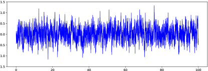
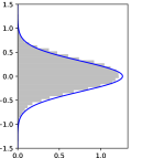
Figure 1.1: Left: Sample path of the diffusion process $\mathrm{d}\zeta_{t}=-10\zeta_{t}\mathrm{d}t+\sqrt{2}\mathrm{d}W_{t}$. Right: Its associated stationary density $\mathrm{N}(0,0.1)$ and the histogram of the sample path.

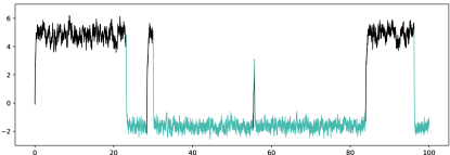
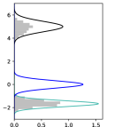
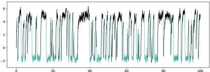
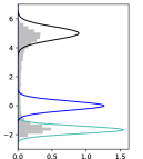
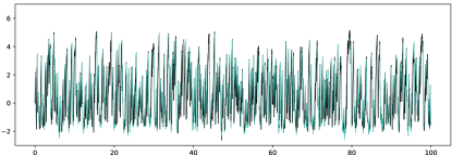
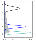
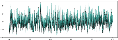
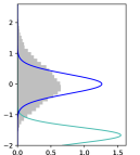
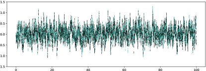
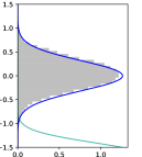
Figure 1.2: Left column: Sample paths of SGLDiffs with $N=2$ given by $\mathrm{d}\theta_{t}=a_{\boldsymbol{i}(t)}(b_{\boldsymbol{i}(t)}-\theta_{t})\mathrm{d}t+\sqrt{2}\mathrm{d}W_{t}$, with $a:=(5,15)$ and $b:=(5,-5/3)$, that approximate SDE and distribution given in Figure 1.1, with $\eta=10^{1},10^{0},10^{-1},10^{-2},10^{-3}$ (top to bottom). We show the path of $(\theta_{t})_{t\geq 0}$ in black whenever $\boldsymbol{i}(t)\equiv 1$ and in teal if $\boldsymbol{i}(t)\equiv 2$. Right column: Stationary densities of subsampled process (e.g., with fixed $\boldsymbol{i}$) in black and teal, respectively, the density of $\mathrm{N}(0,0.1)$ in blue, and the histogram of the sample path in gray.

1.1 Problem setting

Throughout this work, we aim to approximate a probability distribution $\mu$ on a space $X:=\mathbb{R}^{d}$ that we equip with the Euclidean norm $\|\cdot\|$ and its associated Borel-$\sigma$-algebra $\mathcal{B}(X)$. We assume that $\mu$ is given by

$$\mu(\mathrm{d}\theta)=\frac{1}{Z}\exp\left(-{\bar{\Phi}}(\theta)\right)\mathrm{d}\theta,$$

where ${\bar{\Phi}}:=\frac{1}{N}\sum_{i=1}^{N}\Phi_{i}$ is the arithmetic mean of some functions $\Phi_{i}:X\rightarrow\mathbb{R}$ that are bounded below, continuously differentiable, and indexed by $i\in I:=\{1,\ldots,N\}$, and

$$Z:=\int_{X}\exp\left(-{\bar{\Phi}}(\theta^{\prime})\right)\mathrm{d}\theta^{\prime}\in(0,\infty)$$

is the normalising constant. In a Bayesian learning or inference problem, $\mu$ should be thought off as the posterior distribution. In this case, the function $\Phi_{i}$ then refers to the regularised data misfit or the negative log-posterior with respect to the data subset with index $i\in I$. Outside of learning and inference, probability distributions of this form also arise in statistical physics.

We use a Monte Carlo approach to approximate $\mu$, e.g., we generate random samples and then approximate $\mu$ by the associated empirical measure. Here, we rely on MCMC techniques that generate a Markov chain that is ergodic and stationary with respect to $\mu$, e.g., the samples can be used to approximate integrals with respect to $\mu$. An example of a continuous-time Markov chain that does this, is the solution $(\zeta_{t})_{t\geq 0}$ of the following (overdamped) Langevin diffusion:

$$\mathrm{d}\zeta_{t}=-\nabla{\bar{\Phi}}(\zeta_{t})\mathrm{d}t+\sqrt{2}\mathrm{d}W_{t},$$ (1.1)

where $(W_{t})_{t\geq 0}$ is a Brownian motion on $X$. We show an example where the Langevin diffusion is used to approximate a Gaussian distribution in Figure 1.1. In practice, such a Langevin diffusion is used as an inaccurate MCMC algorithm through Euler–Maruyama discretisation. Indeed, this is the unadjusted Langevin algorithm, where the Markov chain $(\widehat{\zeta}_{k})_{k=1}^{\infty}$ is generated by

$$\widehat{\zeta}_{k+1}\leftarrow\widehat{\zeta}_{k}-\eta\nabla{\bar{\Phi}}(\widehat{\zeta}_{k})+\sqrt{2\eta}\xi_{k},$$ (1.2)

where $\eta>0$ is the learning rate (or step size) and $(\xi_{k})_{k=1}^{\infty}$ is a sequence of indendepent and identically distributed (iid) standard Gaussian random variables on $X$. ULA approximates $(\zeta_{t})_{t\geq 0}$, but does not necessarily converge to $\mu$ in its longterm limit.

In practice, $N$ might be very large in which case we may not be able to repeatedly evaluate all $N$ gradients in (1.2). Based on the popular Stochastic Gradient Descent method in optimisation [39], Welling and Teh [42] have proposed the Stochastic Gradient Langevin Dynamic, which is of the form

$$\tilde{\zeta}_{k+1}\leftarrow\tilde{\zeta}_{k}-\eta\nabla\Phi_{i(k)}(\tilde{\zeta}_{k})+\sqrt{2\eta}\xi_{k},$$ (1.3)

where $i(0),i(1),\ldots\sim\mathrm{Unif}(I)$ are iid. This data subsampling that allows us to consider only one gradient at a time introduces again an additional error. In this work, we aim to study this subsampling error, isolatedly from the ULA error. This allows us to obtain a best case error for Langevin-based MCMC methods that are subject to subsampling and is independent from the discretisation. To do so, we will consider the aforementioned Stochastic Gradient Langevin Diffusion, a switched diffusion process that is given through the following dynamical system

$$\mathrm{d}\theta_{t}=-\nabla\Phi_{\boldsymbol{i}(t/\eta)}(\theta_{t})\mathrm{d}t+\sqrt{2}\mathrm{d}W_{t},$$ (1.4)

where $(\boldsymbol{i}(t))_{t\geq 0}$ is a homogeneous continuous-time Markov process on $I$ that jumps from any state to any other state at rate $1$ and where $\eta>0$ still has the character of a learning rate. The definition of the SGLDiff is especially motivated by earlier work on continuous-time stochastic gradient descent [22, 24, 25, 29] and different from purely diffusion-based analyses, e.g., such similar to [31]. We give examples for sample paths of SGLDiff with different learning rates $\eta$ in Figure 1.2. There, we especially illustrate that SGLDiff $(\theta_{t})_{t\geq 0}$ approximates the Langevin diffusion $(\zeta_{t})_{t\geq 0}$, if $\eta\downarrow 0$. Moreover, we can see that SGLDiff also approximates our distribution of interest $\mu$. Throughout this work, we study this approximation of $(\zeta_{t})_{t\geq 0}$ using $(\theta_{t})_{t\geq 0}$.

1.2 Contributions and outline

We now state the contributions of this work and then give an outline.

From a learning perspective, we study the approximation of the Langevin diffusion $(\zeta_{t})_{t\geq 0}$ using SGLDiff $(\theta_{t})_{t\geq 0}$. Indeed,

• we study convergence and divergence between $\theta_{t}$ and $\zeta_{t}$ for small $\eta$ and large $t$, respectively,

• we give assumptions under which SGLDiff has a unique stationary distribution $\mu^{\eta}$ and is ergodic, and we prove an error bound between $\mu$ and $\mu^{\eta}$, and

• we use the triangle inequality to then also bound the distance between $(\theta_{t})_{t\geq 0}$ and $\mu$, giving us information about bias and convergence at the same time.

From a probabilistic perspective, we develop a novel approach by leveraging the key ideas embedded within the ergodic theorem and show the strong convergence between $(\theta_{t})_{t\geq 0}$ and $(\zeta_{t})_{t\geq 0}$ while only having weak convergence between their coefficients $\nabla\Phi_{i(t/\eta)}$ and $\nabla\bar{\Phi}$. We adapt the reflection coupling method in the context of switching diffusion processes and propose an innovative application of this method to address the convergence between the invariant measures of systems (1.1) and (1.4).

We formulate the main results of this work in Theorems 1.1–1.3 in Subsection 1.3 and bring them into context with discrete-in-time results in Subsection 1.4. We outline the proofs of Theorem 1.1 and Theorems 1.2–1.3 in Sections 2 and 3 and make them rigorous in Appendices A and B, respectively. We conclude the work in Section 4 and point the reader towards related open problems.

1.3 Main results

We present our main results in this section – starting with two assumptions.

Assumptions 1.1 (Smoothness)

For any $i\in I$, $\Phi_{i}\in\mathcal{C}^{1}(X:\mathbb{R})$, i.e., it is continuously differentiable. In addition, $\nabla\Phi_{i}$ is Lipschitz continuous with Lipschitz constant $L$, i.e., for any $x,y\in X$,

$$\left\|\nabla\Phi_{i}(x)-\nabla\Phi_{i}(y)\right\|\leq L\left\|x-y\right\|.$$

Assumptions 1.2

There exist $K,R>0$ such that for any $i\in I$ and $\left\|x-y\right\|\geq R,$

$$\left\langle\nabla\Phi_{i}(x)-\nabla\Phi_{i}(y),x-y\right\rangle\geq K\left\|x-y\right\|^{2}.$$

Assumption 1.1 is usual in the literature [38, 44, 52] and provides existence and uniqueness of the solution to the equation (1.4), see, e.g., [43] or [45, Chapter 2]. Note that the solution is $\mathcal{F}^{\eta}_{t}:=\sigma(\mathcal{F}^{B}_{t}\cup\mathcal{F}^{I}_{t/\eta})$-adapted, where $\mathcal{F}^{B}_{t}$ is the filtration generated by the Brownian motion $(W_{t})_{t\geq 0}$ and $\mathcal{F}^{I}_{t}$ is the filtration generated the Markov jump process $(\boldsymbol{i}(t))_{t\geq 0}$. Assumption 1.2 is motivated by [16] and [17], which allows us to use the reflection coupling method to prove exponential convergence. Intuitively, it states that $\Phi_{i}$ is strongly convex if $x$ and $y$ are away from each other. We remark that while this assumption is weaker than strong convexity, it is stronger than the dissipativeness assumption, which is usually assumed in the discrete-in-time literature for convergence analysis of the non-convex case (e.g. [38, 44, 52]). See Appendix C where we discuss this connection.

With the above assumptions, we show three convergence results regarding SGLDiff. We begin by showing that the processes $(\zeta_{t})_{t\geq 0}$ and $(\theta_{t})_{t\geq 0}$ may diverge as $t\rightarrow\infty$, but strongly converge at any fixed time $t$ if the learning rate $\eta\downarrow 0$.

Theorem 1.1

Let $(\theta_{t})_{t\geq 0}$ be the solution to (1.4) and $(\zeta_{t})_{t\geq 0}$ be the solution to (1.1) with initial value $\theta_{0}=\zeta_{0}$. Under Assumptions 1.1, we have the following inequality

$$\mathbb{E}[\left\|\theta_{t}-\zeta_{t}\right\|]\leq C_{\Phi,\theta_{0},d}\mathrm{e}^{8(1+L)t}\eta^{\frac{1}{4}},$$

where $C_{\Phi,\theta_{0},d}=8(1+d+\left\|\theta_{0}\right\|^{2}+2\left\|\nabla\bar{\Phi}(0)\right\|^{2})C^{(1)}_{\Phi}$ and $C^{(1)}_{\Phi}=1+L+\sup_{i\in I}\left\|\nabla\Phi_{i}(0)\right\|.$

One can see easily, that $C_{\Phi,\theta_{0},d}=\mathcal{O}(d)$ in terms of its dependence on the dimension $d$ of $X$.

Next, we study the ergodicity of the SGLDiff (1.4), which we study in terms of the Wasserstein distance. The Wasserstein distance between two probability measures $\nu$ and $\nu^{\prime}$ on $(X,\mathcal{B}(X))$ is given by

$${{\mathcal{W}}}_{\left\|\cdot\right\|}(\nu,\nu^{\prime})=\inf_{\Gamma\in\mathcal{H}(\nu,\nu^{\prime})}\int_{X\times X}\left\|y-y^{\prime}\right\|\Gamma(\mathrm{d}y,\mathrm{d}y^{\prime}),$$

where $\mathcal{H}(\nu,\nu^{\prime})$ is the set of coupling between $\nu$ and $\nu^{\prime}$, i.e.

$$\mathcal{H}(\nu,\nu^{\prime})=\{\Gamma\in\mathrm{Pr}(X\times X):\Gamma(A\times X)=\nu(A),\Gamma(X\times B)=\nu^{\prime}(B)(A,B\in\mathcal{B}(X))\}.$$

We note that Assumptions 1.1 and 1.2 imply that the joint process $(\theta_{t},\boldsymbol{i}(t))_{t\geq 0}$ defined in equation (1.4) is Markovian and admits a unique invariant measure $M^{\eta}(\mathrm{d}\theta,\{i\}).$ We denote by $\mu^{\eta}(\mathrm{d}\theta):=M^{\eta}(\mathrm{d}\theta,I)$ the $(\theta_{t})_{t\geq 0}$-marginal of the stationary distribution $M^{\eta}$ and, similarly, the distributions $\nu_{t}^{\eta}:=\mathbb{P}(\theta_{t}\in\cdot)$ and $\nu_{t}:=\mathbb{P}(\zeta_{t}\in\cdot)$ at a fixed time $t>0$. Finally, we assume in the following that $\boldsymbol{i}(0)\sim\mathrm{Unif}(I)$ and then obtain the following ergodic theorem.

Theorem 1.2

Under the Assumptions 1.1 and 1.2, we have

$$\mathcal{W}_{\left\|\cdot\right\|}(\nu^{\eta}_{t},\mu^{\eta})\leq C\mathrm{e}^{-ct}\mathcal{W}_{\left\|\cdot\right\|}(\nu_{0},\mu^{\eta}),$$

where $c=\min\{\big{(}3L+\frac{2}{R^{2}}\big{)},K\}\mathrm{e}^{-{LR^{2}}/{2}}$ and $C=2\mathrm{e}^{{LR^{2}}/{2}}$.

Theorem 1.2 provides a quantitative way to measure the distance between $\nu_{t}^{\eta}$ and the limiting measure, i.e. the exponential convergence between $\nu_{t}^{\eta}$ and $\mu^{\eta}$. Notice that the constants in the obtained upper bound are independent of the dimension as the reflection coupling reduces the diffusion to a one-dimensional Brownian motion, which will be explained later in the outline of the proof.

In the third convergence result, we study the invariant measures $\mu$ and $\mu^{\eta}$ of $(\zeta_{t})_{t\geq 0}$ and $(\theta_{t})_{t\geq 0}$. Here, we bound the Wasserstein distance between $\mu$ and $\mu^{\eta}$ and, thus, quantify the asymptotic subsampling error between correct distribution and SGLDiff.

Theorem 1.3

Under the Assumptions 1.1 and 1.2, the marginal distribution $\mu^{\eta}(dx)$ converges weakly to the stationary measure of $(\zeta_{t})_{t\geq 0}$. In particular, we have

$$\mathcal{W}_{\left\|\cdot\right\|}(\mu^{\eta},\mu)\leq C_{\Phi,d}\eta^{c_{\Phi}},$$

where $c_{\Phi}:=\frac{c}{32(L+1)+4c}$ and $C_{\Phi,d}:=C_{\Phi,\theta_{0}=0,d}+C^{(1)}_{d}C,$ with $C^{(1)}_{d}=\mathcal{O}(\sqrt{d}).$

When $t$ goes to infinity, both, $(\zeta_{t})_{t\geq 0}$ and $(\theta_{t})_{t\geq 0}$ converge to their invariant measures respectively, and this theorem shows that their invariant measures coincide as the learning rate goes to zero. From Theorem 1.1, we know that the dimension-dependence of the constant $C_{\Phi,d}$ is of order $\mathcal{O}(d)$. The rate $c_{\Phi}$ is approximately $1/4-\delta$ for some $\delta>0$ and dimension-independent. The constant $C^{(1)}_{d}$ is discussed explicitly in Lemma 3.1.

1.4 Comparison with discrete-in-time Langevin algorithm and related work

There has been an increasing interest in the use of Langevin diffusion-based algorithms for the approximation of Bayesian posterior distributions as these algorithms have demonstrated significant potential for achieving accurate and efficient sampling [42]. The convergence rate has been studied extensively under different log-concavity conditions on the target distribution, see for example [9, 10, 13, 14, 34]; as well as in the non-log-concave case, see for example, [1, 30, 32, 38, 41, 44]. In recent years, there has been a growing body of research focused on improving and extending Langevin diffusion-based algorithms for Bayesian sampling. The subsampling-variant of the unadjusted Langevin algorithm, referred to as Stochastic Gradient Langevin Dynamics (SGLD), has proven to be particularly useful for sampling and optimization tasks in which the objective function is nonconvex, noisy, and/or has a large number of parameters. Recall that the Stochastic Gradient Langevin Dynamics updates are defined as in (1.3). The convergence rate of this algorithm and its variants have been studied in for example, [6, 11, 21, 38, 44, 46, 52]. Since then, a significant amount of effort has been put into improving various aspects. For example, SGLD can be combined with variance reduction resulting in a faster convergence rate, such as the Stochastic Variance Reduced Gradient Langevin Dynamics (SVRG-LD), see for instance, [12, 23, 27, 44, 49, 50, 52]. Another direction of work are higher order MCMC methods, such as Hamiltonian Monte Carlo (see e.g. non-subsampling: [3, 7, 15, 33, 35, 37], subsampling: [47]) and the underdamped Langevin dynamics (see e.g. non-subsampling: [8, 17, 19], subsampling: [4, 5, 21, 48, 51]).

In particular, the vanilla SGLD in the context of non-convex learning converges as,

$${{\mathcal{W}}}_{2}(\mathbb{P}(\tilde{\zeta}_{k}\in\cdot),\mu)=\mathcal{O}\big{(}(1+d)(\delta^{1/4}+\eta^{1/4})k\eta\big{)}+\mathcal{O}\left(\frac{1+d}{\sqrt{\lambda}}\right)\mathrm{e}^{-\Omega(\lambda k\eta/(d+1))},$$

where ${{\mathcal{W}}}_{2}:=({{\mathcal{W}}}_{\left\|\cdot\right\|^{2}})^{1/2}$ is the Wasserstein-2 distance, $d$ is still the dimension of $X$, $\lambda$ is the uniform spectral gap of the limiting measure $\mu$, and $\delta$ bounds the second moment of stochastic gradient noise; see [38] for details. Note that this bound has been improved in [52]. Even though a direct comparison between our result and this bound may not be possible, it is still noteworthy to observe the discrete analogy of our continuous scenario, which offers interesting insights. Using the triangle inequality to combine Theorems 1.2 and 1.3, we have

$$\mathcal{W}_{\left\|\cdot\right\|}(\nu_{t}^{\eta},\mu)\leq C_{\Phi,d}\eta^{c_{\Phi}}+C\mathrm{e}^{-ct}\mathcal{W}_{\left\|\cdot\right\|}(\nu_{0},\mu^{\eta}),$$

where $C_{\Phi,d}$ is of order $\mathcal{O}(d)$. The first term is independent of time, however $c_{\Phi}\leq 1/4$ indicates slow convergence. The second term decays exponentially in time and it is independent of the dimension $d$. Hence, our analysis indicates that the subsampling error in SGLDiff is not amplified as time $t\rightarrow\infty$, although in our result converging slower as a function of $\eta$ compared to SGLD. Moreover, the ergodic convergence rate is dimension independent in our idealised setting. Both results indicate that one may be able to find a Langevin-based subsampling MCMC method that significantly improves upon SGLD.

2 SGLDiff $(\theta_{t})_{t\geq 0}$ approximates the Langevin diffusion $(\zeta_{t})_{t\geq 0}$

In this section, we give a sketch of the proof of Theorem 1.1 showing the strong convergence of $\theta_{t}\rightarrow\zeta_{t}$ for a fixed time $t>0$, as $\eta\downarrow 0$. The full proof of this theorem and proofs of auxiliary results stated here are deferred to Appendix A. The proof of Theorem 1.1 is inspired by the calculation of the variance for ergodic averages, for example, see [18, Chapter 2.2] and [28]. We notice that $\boldsymbol{i}(\cdot/\eta)$ converges weakly to its invariant measure when $\eta\downarrow 0$. From the ergodic theory for Markov processes, however, we expect that $\int_{0}^{t}\nabla\Phi_{\boldsymbol{i}(s/\eta)}(\theta_{s})ds=\eta\int_{0}^{t/\eta}\nabla\Phi_{\boldsymbol{i}(r)}(\theta_{\eta r})dr$ converges to $\int_{0}^{t}\nabla\bar{\Phi}(\theta_{s})ds$ strongly, which we can then use to prove strong convergence of the full processes. Before sketching the proof of Theorem 1.1, we require some auxiliary results. We start with the following.

Lemma 2.1

Under Assumption 1.1, for any $t>0,$ we have the following inequality,

$$\mathbb{E}[\left\|\zeta_{t}\right\|^{2}]\leq\tilde{c}_{t,\theta_{0},d},$$

where $\tilde{c}_{t,\theta_{0},d}=\Big{(}\left\|\theta_{0}\right\|^{2}+2\left\|\nabla\bar{\Phi}(0)\right\|^{2}+2td\Big{)}\mathrm{e}^{2(L+1)t}.$

Lemma 2.1 provides the boundedness of $(\zeta_{t})_{t\geq 0}$ which will be used repeatedly in the rest of the paper. The following Lemma shows that $(\zeta_{t})_{t\geq 0}$ is continuous in time due to the continuity from the drift and the Brownian motion. This continuity allows us to employ a time decomposition later in the proof of Theorem 1.1.

Lemma 2.2

Under Assumption 1.1, $(\theta_{t})_{t\geq 0}$ is continuous w.r.t time, in the following sense: for $t>s>0,$ we have

$$\mathbb{E}[\left\|\zeta_{t}-\zeta_{s}\right\|^{2}]\leq c_{t,\theta_{0},d}\left|t-s\right|,$$

where $c_{t,\theta_{0},d}:=2\mathrm{e}^{2(L+1)t}\tilde{c}_{t,\theta_{0},d}.$

Notice that the Markov process $(\boldsymbol{i}(t))_{t\geq 0}$ is ergodic, i.e.

$$\frac{1}{T}\int_{0}^{T}g_{\boldsymbol{i}(t)}dt\to\frac{1}{N}\sum^{N}_{i=1}g_{i},$$

as $T\rightarrow\infty$, for some function $g:I\rightarrow X$. The following lemma discusses the precise convergence rate and shows that the time average converges to the space-average with order $\mathcal{O}(1/\sqrt{T})$.

Lemma 2.3

Let $g:I\rightarrow X$ satisfy $\sum_{i=1}^{N}g_{i}=0$. Then

$$\sup_{\boldsymbol{i}(0)\in I}\mathbb{E}_{\boldsymbol{i}(0)}\Big{[}\left\|\int_{0}^{\frac{t}{\eta}}g_{\boldsymbol{i}(s)}\mathrm{d}s\right\|^{2}\Big{]}\leq\frac{2\max_{i=1,...,N}\left\|g_{i}\right\|^{2}}{N}\frac{t}{\eta}\ .$$

We now have all ingredients to explain how Theorem 1.1 can be proven.

Proof sketch of Theorem 1.1

In the proof of Theorem 1.1, the main idea is to break down the difference of $\theta_{t}$ and $\zeta_{t}$. First, we examine equations (1.1) and (1.4) and rewrite $\left\|\theta_{t}-\zeta_{t}\right\|$ by inserting $\nabla\Phi_{\boldsymbol{i}(s/\eta)}(\zeta_{s})$ between $\nabla\Phi_{\boldsymbol{i}(s/\eta)}(\theta_{s})$ and $\nabla\bar{\Phi}(\zeta_{s})$. Indeed, we employ

$$\left\|\theta_{t}-\zeta_{t}\right\|= \left\|\int_{0}^{t}\nabla\Phi_{\boldsymbol{i}(s/\eta)}(\theta_{s})-\nabla\bar{\Phi}(\zeta_{s})\mathrm{d}s\right\|$$

$$\leq \left\|\int_{0}^{t}\nabla\Phi_{\boldsymbol{i}(s/\eta)}(\theta_{s})-\nabla\Phi_{\boldsymbol{i}(s/\eta)}(\zeta_{s})\mathrm{d}s\right\|+\left\|\int_{0}^{t}\nabla\Phi_{\boldsymbol{i}(s/\eta)}(\zeta_{s})-\nabla\bar{\Phi}(\zeta_{s})\mathrm{d}s\right\|.$$

For the term $\nabla\Phi_{\boldsymbol{i}(s/\eta)}(\theta_{s})-\nabla\Phi_{\boldsymbol{i}(s/\eta)}(\zeta_{s})$, we apply the Lipschitz assumption from Assumption 1.1. Consequently, $\left\|\theta_{t}-\zeta_{t}\right\|$ can be bounded by the sum of $\int_{0}^{t}\left\|\theta_{s}-\zeta_{s}\right\|\mathrm{d}s$ and $\left\|\int_{0}^{t}\nabla\Phi_{\boldsymbol{i}(s/\eta)}(\zeta_{s})-\nabla\bar{\Phi}(\zeta_{s})\mathrm{d}s\right\|$. Our main goal is to show that the second term is bounded by a constant depending on $t\eta^{1/4}$. To achieve this, we use a discretization technique to estimate the integral ([28] and [25, proof of Theorem 3]). More precisely, one can understand the switching rate $\eta$ as the discretization time-step and analyze the difference on each time interval of length $\tilde{\eta}$,

$$\int_{0}^{t}\nabla\Phi_{\boldsymbol{i}(s/\eta)}(\zeta_{s})-\nabla\bar{\Phi}(\zeta_{s})\mathrm{d}s=\sum^{1/\tilde{\eta}}_{j=1}\int_{(j-1)t\tilde{\eta}}^{jt\tilde{\eta}}\nabla\Phi_{\boldsymbol{i}(s/\eta)}(\zeta_{s})-\nabla\bar{\Phi}(\zeta_{s})\mathrm{d}s.$$

Within each time interval $((j-1)t\tilde{\eta},jt\tilde{\eta}]$ we want to control the variation of $(\zeta_{t})_{t\geq 0}$ (using Lemma 2.2), which requires the length $\tilde{\eta}$ to be small. On the other hand, using the ergodicity bound from Lemma 2.3, the fluctuation on each interval has to be large enough so that the overall sum goes to zero. Consequently, we choose $\tilde{\eta}$ approximately to be $\sqrt{\eta}$, which optimally satifies those requirements. Once this bound is established, we apply Grönwall’s inequality to obtain the desired result.

3 The stationary distribution $\mu^{\eta}$ approximates $\mu$

We now study how well $\mu^{\eta}$ approximates $\mu$. Again, the full proofs of the main theorems and lemmas are deferred to Appendix B. We begin by showing that $(\theta_{t})_{t\geq 0}$ converges exponentially to its stationary measure.

Proof sketch of Theorem 1.2

Before discussing the proof of Theorem 1.2, we recall the exponential contractivity for Markov semi-groups (see e.g. [29, 18, 16]). Let $p_{t}:X\times\mathcal{B}(X)\rightarrow[0,1]$ be a homogeneous Markov semi-group and let $\pi$ be its invariant measure. The exponential contraction in Wasserstein distance induced by some distance $d$ is defined as

$$\mathcal{W}_{d}(\pi_{0}p_{t},\pi)\leq\mathrm{e}^{-ct}\mathcal{W}_{d}(\pi_{0},\pi).$$

Now, while the pair $(\theta_{t},\boldsymbol{i}(t/\eta))_{t\geq 0}$ is a Markov process, $(\theta_{t})_{t\geq 0}$ on its own is not Markovian. Rather than exploring the contractivity of the pair $(\theta_{t},\boldsymbol{i}(t/\eta))_{t\geq 0}$, we start the dynamic with $\boldsymbol{i}(0)$ being already distributed according to its invariant measure $\mathrm{Unif}(I)$ and study the contractivity only in $(\theta_{t})_{t\geq 0}$. When the potentials $(\Phi_{i})_{i\in I}$ are strongly convex, this property is classical and we could use the method in e.g. [29] to obtain it. More precisely, one can construct a coupled process starting from the invariant measure and run the same dynamic with the same diffusion process. However, in the non-convex case, we do not obtain enough decay solely from the potential hence we need to construct the coupling in a way such that the diffusion term offers extra decay. By selecting an appropriate distance function $F(\cdot)$, it is possible to achieve exponential contractivity even in non-convex potential cases. Here, we choose the distance function to be a supermartingale w.r.t $\mathcal{F}_{t}^{\eta}$ and equivalent to the Euclidean distance so that we get exponential decay under this distance and deduce the exponential decay in $\left\|\cdot\right\|$. This idea is adapted from the reflection couplings discussed by [16, 17]. Intuitively, by diffusing the coupled process along the reflection, we compensate for the lack of decay in the drift. As a result, a large exponential decay rate can be obtained in the $\mathcal{W}_{\left\|\cdot\right\|}$ distance.

Now, we move on to show the error bound between the stationary distribution $\mu^{\eta}$ and the distribution of interest $\mu$.

Proof sketch of Theorem 1.3

The following lemma shows that $\mu^{\eta}$ and $\mu$ are bounded in terms of their first absolute moments. Recall that $\mu^{\eta}$ is the marginal distribution of the invariant measure of $(\theta_{t})_{t\geq 0}$ and $\mu$ is the invariant measure of $(\zeta_{t})_{t\geq 0}$.

Lemma 3.1

Let $\delta_{0}$ be the Dirac delta function at $0$. Under Assumptions 1.1 and 1.2, we have

$$\mathcal{W}_{\left\|\cdot\right\|}(\delta_{0},\mu^{\eta})\leq C^{(1)}_{d},$$

where $C^{(1)}_{d}=\sqrt{C_{\Phi}K^{-1}d}$ and $C_{\Phi}=2(L+K)R^{2}+\sup_{i\in I}\frac{\left\|\nabla\Phi_{i}(0)\right\|^{2}}{K}.$

Specifically, when $N=1$, it is easy to conclude that

$$\mathcal{W}_{\left\|\cdot\right\|}(\delta_{0},\mu)\leq C^{(1)}_{d}.$$

We first insert $\nu^{\eta}_{t}$ and $\nu_{t}$ into the distance between $\mu^{\eta}$ and $\mu$. Using the triangle inequality, we find that $\mathcal{W}_{\left\|\cdot\right\|}(\mu^{\eta},\mu)$ can be bounded by the sum of three terms: $\mathcal{W}_{\left\|\cdot\right\|}(\mu^{\eta},\nu^{\eta}_{t})$, $\mathcal{W}_{\left\|\cdot\right\|}(\nu^{\eta}_{t},\nu_{t})$, and $\mathcal{W}_{\left\|\cdot\right\|}(\nu_{t},\mu)$,

$$\mathcal{W}_{\left\|.\right\|}(\mu^{\eta},\mu)\leq\mathcal{W}_{\left\|.\right\|}(\mu^{\eta},\nu^{\eta}_{t})+\mathcal{W}_{\left\|.\right\|}(\nu^{\eta}_{t},\nu_{t})+\mathcal{W}_{\left\|.\right\|}(\nu_{t},\mu).$$

Essentially, the distance between the invariant measures propagates through the distance between their dynamics, $\mathcal{W}_{\left\|\cdot\right\|}(\nu^{\eta}_{t},\nu_{t})$. Assuming they have the same initial value, this can be controlled using Theorem 1.1 and we obtain an upper bound of order $\eta^{1/4}$. Starting at $0$, from Theorem 1.2, we can bound $\mathcal{W}_{\left\|\cdot\right\|}(\mu^{\eta},\nu^{\eta}_{t})$ and $\mathcal{W}_{\left\|\cdot\right\|}(\nu_{t},\mu)$ by $\mathcal{W}_{\left\|\cdot\right\|}(\delta_{0},\mu^{\eta})+\mathcal{W}_{\left\|\cdot\right\|}(\delta_{0},\mu)$ with exponential decay, which are bounded due to Lemma 3.1. Hence the distance between the dynamic and its invariant measure is bounded in both (1.1) and (1.4). Since the left-hand side is independent of $t$, we choose $t$ freely to obtain an optimal bound. While the contractivity is obtained for each dynamic and their limiting measures, the distance between the dynamics accumulates as $t$ goes to infinity, and the precise rate is given in Theorem 1.1. Hence, we design $t$ as a function of $\eta$ such that the overall bound goes to $0$ as $\eta$ goes to $0$.

4 Conclusions and open problems

Our analysis has shown that our idealised subsampling MCMC dynamic SGLDiff is able to approximate the distribution of interest $\mu$ at high accuracy. We especially learnt that the convergence rate is dimension-independent, only the prefactors depend linearly on the dimension of the sample space. Our analysis also shows that the amplification of the subsampling error throughout time is a numerical artefact introduced by the Euler–Maruyama discretisation of ULA. Hence, this amplification may be prevented or reduced with a more accurate or more stable discretisation scheme.

Whilst it may be possible to find better algorithms for the sampling of posterior (and other) distributions in large-scale data settings, our work does not give a recipe to find such a technique. A clear limitation of our approach is that it relies on an idealised dynamical system. In addition, the obtained fractional rate $<1/4$ may be too slow for many practical applications.

To the best of our knowledge, we are not aware of any negative social impacts in our results.

4.1 Future work

There are many related open problems. We discuss two next steps below.

Optimisation.

SGLD can also be seen as a noisier version of the Stochastic Gradient Descent method [39], where additional Gaussian noise is added to the stochastic gradients to further regularize the optimisation problem. In this case, we would probably consider equation (1.4) with an inverse temperature $\beta>0$, i.e.

$$\mathrm{d}\theta_{t}=-\nabla\Phi_{\boldsymbol{i}(t/\eta)}(\theta_{t})\mathrm{d}t+\sqrt{2\beta^{-1}}\mathrm{d}W_{t}.$$ (4.1)

The non-subsampled version of this equation (i.e. setting $\Phi_{\boldsymbol{i}(t/\eta)}={\bar{\Phi}}$) has invariant distribution $\mu_{\beta}(\mathrm{d}\theta)\propto\mathrm{e}^{-\Phi(\theta)/\beta}\mathrm{d}\theta.$ With certain assumptions on the potential function ${\bar{\Phi}}$, $\mu^{\beta}$ converges to $\delta_{\theta_{*}}$ weakly as $\beta\to\infty$, where $\delta_{\theta_{*}}$ is the Dirac delta function concentrated in the global minimizer $\theta_{*}$ of ${\bar{\Phi}}$. We may now study the invariant distribution $\mu^{\eta}_{\beta}$ of the subsampled process $(\theta_{t})_{t\geq 0}$ that solves (4.1). Here, we especially ask, whether $\mu^{\eta}_{\beta}\rightarrow\delta_{\theta_{*}}$, if $\beta\uparrow\infty$ and $\eta\downarrow 0$. And thus, whether and how fast this noisier version of Stochastic Gradient Descent can find the global optimiser of ${\bar{\Phi}}$.

Momentum.

Higher-order dynamics have shown to be very successful at optimisation, e.g. ADAM [26], and sampling, e.g. the previously mentioned Hamiltonian Monte Carlo. In our work, we can obtain a higher-order dynamic by including a momentum term in equation (1.4) and, thus, obtain an underdamped Stochastic Gradient Langevin Diffusion

$$\mathrm{d}X_{t}= V_{t}\mathrm{d}t$$

$$\mathrm{d}V_{t}= -\gamma V_{t}\mathrm{d}t-\nabla\Phi_{\boldsymbol{i}(t/\eta)}(X_{t})\mathrm{d}t+\sqrt{2}\mathrm{d}W_{t},$$

for which we would study the convergence of the solution $(X_{t})_{t\geq 0}$ analogous to that of $(\theta_{t})_{t\geq 0}$. The momentum may help to explore complicated energy landscapes in Bayesian deep learning and may reduce the influence of the subsampling. Ideas from [24] might help the analysis.

Appendix for Subsampling Error in Continuous Stochastic Gradient Langevin Dynamics

Appendix A Proof of Theorem 1.1

A.1 Proof of Lemma 2.1

Lemma 2.1 Under Assumption 1.1, for any $t>0,$ we have the following inequality,

$$\mathbb{E}[\left\|\zeta_{t}\right\|^{2}]\leq\tilde{c}_{t,\theta_{0},d},$$

where $\tilde{c}_{t,\theta_{0},d}=\Big{(}\left\|\theta_{0}\right\|^{2}+2\left\|\nabla\bar{\Phi}(0)\right\|^{2}+2td\Big{)}e^{2(L+1)t}.$

• By Itô’s formula, we have

  $$\frac{\left\|\zeta_{t}\right\|^{2}}{2}= \left\|\theta_{0}\right\|^{2}-\int_{0}^{t}\left\langle\zeta_{s},\nabla\bar{\Phi}(\zeta_{s})\right\rangle\mathrm{d}t+\sqrt{2}\int_{0}^{t}\left\langle\zeta_{s},\mathrm{d}B_{s}\right\rangle+td$$

  $$= \left\|\theta_{0}\right\|^{2}-\int_{0}^{t}\left\langle\zeta_{s},\nabla\bar{\Phi}(\zeta_{s})-\nabla\bar{\Phi}(0)\right\rangle\mathrm{d}s$$

  $$-\int_{0}^{t}\left\langle\zeta_{s},\nabla\bar{\Phi}(0)\right\rangle\mathrm{d}s+\sqrt{2}\int_{0}^{t}\left\langle\zeta_{s},\mathrm{d}B_{s}\right\rangle+td$$

  $$\leq \left\|\theta_{0}\right\|^{2}+L\int_{0}^{t}\left\|\zeta_{s}\right\|^{2}\mathrm{d}s+\left\|\nabla\bar{\Phi}(0)\right\|\int_{0}^{t}\left\|\zeta_{s}\right\|\mathrm{d}s+\sqrt{2}\int_{0}^{t}\left\langle\zeta_{s},\mathrm{d}B_{s}\right\rangle+td$$

  $$\leq \left\|\theta_{0}\right\|^{2}+(L+1)\int_{0}^{t}\left\|\zeta_{s}\right\|^{2}\mathrm{d}s+\left\|\nabla\bar{\Phi}(0)\right\|^{2}+\sqrt{2}\int_{0}^{t}\left\langle\zeta_{s},\mathrm{d}B_{s}\right\rangle+td.$$

  Taking expectation of both sides, we have

  $$\frac{\mathbb{E}[\left\|\zeta_{t}\right\|^{2}]}{2}\leq\frac{\left\|\theta_{0}\right\|^{2}}{2}+(L+1)\int_{0}^{t}\mathbb{E}[\left\|\zeta_{s}\right\|^{2}]\mathrm{d}s+\left\|\nabla\bar{\Phi}(0)\right\|^{2}+td.$$

  By using Grönwall’s inequality, we obtain the bound

  $$\mathbb{E}[\left\|\zeta_{t}\right\|^{2}]\leq\Big{(}\left\|\theta_{0}\right\|^{2}+2\left\|\nabla\bar{\Phi}(0)\right\|^{2}+td\Big{)}e^{2(L+1)t},$$

  which completes the proof. $\hfill\Box$

A.2 Proof of Lemma 2.2

Lemma 2.2 Under Assumption 1.1, $(\theta_{t})_{t\geq 0}$ is continuous w.r.t time, in the following sense: for $t>s>0,$ we have

$$\mathbb{E}[\left\|\zeta_{t}-\zeta_{s}\right\|^{2}]\leq c_{t,\theta_{0},d}\left|t-s\right|,$$

where $c_{t,\theta_{0},d}:=2\mathrm{e}^{2(L+1)t}\tilde{c}_{t,\theta_{0},d}.$

• From equation (1.1), we get

  $$\left\|\zeta_{t}-\zeta_{s}\right\|\leq\underbrace{\int_{s}^{t}\left\|\nabla\bar{\Phi}(\zeta_{r})\right\|\mathrm{d}r}_{(m2.1)}+\underbrace{\sqrt{2}\left\|B_{t}-B_{s}\right\|}_{(m2.2)}.$$

  The second term can be bounded by the variance of increments of Brownian motions,

  $$\mathbb{E}\Big{[}(m2.2)^{2}\Big{]}=2\left|t-s\right|.$$

  Consider the first term,

  $$(m2.1)=\int_{s}^{t}\left\|\nabla\bar{\Phi}(\zeta_{r})\right\|\mathrm{d}r= \int_{s}^{t}(\left\|\nabla\bar{\Phi}(\zeta_{r})-\nabla\bar{\Phi}(0)\right\|+\left\|\nabla\bar{\Phi}(0)\right\|)\mathrm{d}r$$

  $$\leq L\int_{s}^{t}\left\|\zeta_{r}\right\|\mathrm{d}r+\left\|\nabla\bar{\Phi}(0)\right\|\left|t-s\right|.$$

  By Lemma 2.1, we conclude

  $$\mathbb{E}[\left|(m2.1)\right|^{2}]\leq 2(\tilde{c}_{t,\theta_{0},d}+\left\|\nabla\bar{\Phi}(0)\right\|^{2})t\left|t-s\right|,$$

  which yields

  $$\mathbb{E}[\left\|\zeta_{t}-\zeta_{s}\right\|^{2}]\leq 2\mathbb{E}[\left|(m2.1)\right|^{2}]+2\mathbb{E}[\left|(m2.2)\right|^{2}]\leq c_{t,\theta_{0},d}\left|t-s\right|$$

  for some constant $c_{t,\theta_{0},d}.$ $\hfill\Box$

A.3 Proof of Lemma 2.3

Lemma 2.3 Let $g:I\rightarrow X$ satisfy $\sum_{i=1}^{N}g_{i}=0$. Then

$$\sup_{\boldsymbol{i}(0)\in I}\mathbb{E}_{\boldsymbol{i}(0)}\Big{[}\left\|\int_{0}^{\frac{t}{\eta}}g_{\boldsymbol{i}(s)}\mathrm{d}s\right\|^{2}\Big{]}\leq\frac{2\max_{i=1,...,N}\left\|g_{i}\right\|^{2}}{N}\frac{t}{\eta}\ .$$

• We rewrite the square integral and use the Markov property of $(\boldsymbol{i}(t))_{t\geq 0}$,

  $$\mathbb{E}_{\boldsymbol{i}(0)}\Big{[}\left\|\int_{0}^{\frac{t}{\eta}}g_{\boldsymbol{i}(s)}\mathrm{d}s\right\|^{2}\Big{]}= \mathbb{E}_{\boldsymbol{i}(0)}\Big{[}\int_{0}^{\frac{t}{\eta}}\int_{0}^{\frac{t}{\eta}}\left\langle g_{\boldsymbol{i}(s)},g_{\boldsymbol{i}(r)}\right\rangle\mathrm{d}s\mathrm{d}r\Big{]}$$

  $$= 2\mathbb{E}_{\boldsymbol{i}(0)}\Big{[}\int_{0}^{\frac{t}{\eta}}\int_{0}^{\frac{t}{\eta}}\left\langle g_{\boldsymbol{i}(s)},g_{\boldsymbol{i}(r)}\right\rangle\boldsymbol{1}_{r\leq s}\mathrm{d}s\mathrm{d}r\Big{]}\textit{ (since $s,r$ are symmetric)}$$

  $$= 2\mathbb{E}_{\boldsymbol{i}(0)}\Big{[}\int_{0}^{\frac{t}{\eta}}\int_{r}^{\frac{t}{\eta}}\left\langle g_{\boldsymbol{i}(s)},g_{\boldsymbol{i}(r)}\right\rangle\mathrm{d}s\mathrm{d}r\Big{]}$$

  $$= 2\mathbb{E}_{\boldsymbol{i}(0)}\Big{[}\int_{0}^{\frac{t}{\eta}}\int_{r}^{\frac{t}{\eta}}\mathbb{E}[\left\langle g_{\boldsymbol{i}(s)},g_{\boldsymbol{i}(r)}\right\rangle|\mathcal{F}_{r}]\mathrm{d}s\mathrm{d}r\Big{]}$$

  $$= 2\mathbb{E}_{\boldsymbol{i}(0)}\Big{[}\int_{0}^{\frac{t}{\eta}}\int_{r}^{\frac{t}{\eta}}\mathbb{E}_{j=\boldsymbol{i}(r)}[\left\langle g_{\boldsymbol{i}(s-r)},g_{j}\right\rangle]\mathrm{d}s\mathrm{d}r\Big{]}\textit{ (by Markov property)}$$

  $$= 2\mathbb{E}_{\boldsymbol{i}(0)}\Big{[}\int_{0}^{\frac{t}{\eta}}\int_{r}^{\frac{t}{\eta}}\frac{1-e^{-N(s-r)}}{N}\underbrace{\left\langle\sum^{N}_{i=1}g_{i},g_{\boldsymbol{i}(r)}\right\rangle}_{=0}+e^{-N(s-r)}\left\|g_{\boldsymbol{i}(r)}\right\|^{2}\mathrm{d}s\mathrm{d}r\Big{]}$$

  $$\left(\frac{1-e^{-N(s-r)}}{N}\textit{is the probability switching from $j$ to any other state in $(s-r,s]$.}\right)$$

  $$= 2\int_{0}^{\frac{t}{\eta}}\int_{r}^{\frac{t}{\eta}}e^{-N(s-r)}\mathbb{E}_{\boldsymbol{i}(0)}[\left\|g_{\boldsymbol{i}(r)}\right\|^{2}]\mathrm{d}s\mathrm{d}r$$

  $$\leq 2\max_{i=1,...,N}\left\|g_{i}\right\|^{2}\int_{0}^{\frac{t}{\eta}}\int_{0}^{\frac{t}{\eta}-r}e^{-Nm}\mathrm{d}m\mathrm{d}r$$

  $$\leq \frac{2\max_{i=1,...,N}\left\|g_{i}\right\|^{2}}{N}\frac{t}{\eta}.$$

  $\hfill\Box$

A.4 Proof of Theorem 1.1

Theorem 1.1 Let $(\theta_{t})_{t\geq 0}$ be the solution to (1.4) and $(\zeta_{t})_{t\geq 0}$ be the solution to (1.1) with initial value $\theta_{0}=\zeta_{0}$. Under Assumption 1.1, we have the following inequality

$$\mathbb{E}[\left\|\theta_{t}-\zeta_{t}\right\|]\leq C_{\Phi,\theta_{0},d}\mathrm{e}^{8(1+L)t}\eta^{\frac{1}{4}},$$

where $C_{\Phi,\theta_{0},d}=8(1+d+\left\|\theta_{0}\right\|^{2}+2\left\|\nabla\bar{\Phi}(0)\right\|^{2})C^{(1)}_{\Phi}$ and $C^{(1)}_{\Phi}=1+L+\sup_{i\in I}\left\|\nabla\Phi_{i}(0)\right\|.$

• We decompose $\left\|\theta_{t}-\zeta_{t}\right\|$ into two terms using equations (1.1) and (1.4),

  $$\left\|\theta_{t}-\zeta_{t}\right\|= \left\|\int_{0}^{t}\nabla\Phi_{\boldsymbol{i}(s/\eta)}(\theta_{s})-\nabla\bar{\Phi}(\zeta_{s})\mathrm{d}s\right\|$$

  $$\leq \left\|\int_{0}^{t}\nabla\Phi_{\boldsymbol{i}(s/\eta)}(\theta_{s})-\nabla\Phi_{\boldsymbol{i}(s/\eta)}(\zeta_{s})\mathrm{d}s\right\|+\left\|\int_{0}^{t}\nabla\Phi_{\boldsymbol{i}(s/\eta)}(\zeta_{s})-\nabla\bar{\Phi}(\zeta_{s})\mathrm{d}s\right\|$$

  $$\leq L\int_{0}^{t}\left\|\theta_{s}-\zeta_{s}\right\|\mathrm{d}s+\left\|\int_{0}^{t}\nabla\Phi_{\boldsymbol{i}(s/\eta)}(\zeta_{s})-\nabla\bar{\Phi}(\zeta_{s})\mathrm{d}s\right\|.$$ (A.1)

  We claim that $\mathbb{E}[\left\|\int_{0}^{t}\nabla\Phi_{\boldsymbol{i}(s/\eta)}(\zeta_{s})-\nabla\bar{\Phi}(\zeta_{s})\mathrm{d}s\right\|]$ can be bounded by $C_{t,\theta_{0},d}\sqrt{\eta}$ for some $C_{t,\theta_{0},d}>0$. Let $\tilde{\eta}:=1/[1/\sqrt{\eta}]$, where $[x]$ is the greatest integer less than or equal to $x$. Then we have the following decomposition

  $$\int_{0}^{t}\Big{(}\nabla\Phi_{\boldsymbol{i}(s/\eta)}(\zeta_{s})-\nabla\bar{\Phi}(\zeta_{s})\Big{)}\mathrm{d}s=\sum^{1/\tilde{\eta}}_{i=1}\int_{(i-1)t\tilde{\eta}}^{it\tilde{\eta}}G(\boldsymbol{i}(s/\eta),\zeta_{s})\mathrm{d}s,$$

  where $G(i,x)=\nabla\Phi_{i}(x)-\nabla\bar{\Phi}(x).$ For fixed $i$, $G(i,x)$ is Lipschitz continuous with constant $L$. Hence,

  $$\left\|\int_{(i-1)t\tilde{\eta}}^{it\tilde{\eta}}(G(\boldsymbol{i}(s/\eta),\zeta_{s})\mathrm{d}s\right\|\leq \left\|\int_{(i-1)t\tilde{\eta}}^{it\tilde{\eta}}(G(\boldsymbol{i}(s/\eta),\zeta_{s})-G(\boldsymbol{i}(s/\eta),\zeta_{(i-1)t\tilde{\eta}}))\mathrm{d}s\right\|$$

  $$+ \left\|\int_{(i-1)t\tilde{\eta}}^{it\tilde{\eta}}(G(\boldsymbol{i}(s/\eta),\zeta_{(i-1)t\tilde{\eta}})\mathrm{d}s\right\|$$

  $$\leq L\underbrace{\int_{(i-1)t\tilde{\eta}}^{it\tilde{\eta}}\left\|\zeta_{s}-\zeta_{(i-1)t\tilde{\eta}}\right\|\mathrm{d}s}_{(p2.1)}+\underbrace{\left\|\int_{(i-1)t\tilde{\eta}}^{it\tilde{\eta}}(G(\boldsymbol{i}(s/\eta),\zeta_{(i-1)t\tilde{\eta}})\mathrm{d}s\right\|}_{(p2.2)}.$$

  By Lemma 2.2, we bound the first term as

  $$\mathbb{E}[(p2.1)]\leq Lc_{t,\theta_{0},d}(t\tilde{\eta})^{\frac{3}{2}}.$$

  We first study the second term whilst conditioning on $\mathcal{F}^{\eta}_{(i-1)t\tilde{\eta}}$,

  $$\mathbb{E}\Big{[}(p2.2)\Big{|}\mathcal{F}^{\eta}_{(i-1)t\tilde{\eta}}\Big{]} =\mathbb{E}_{i^{\eta}((i-1)t\tilde{\eta}),x=\zeta_{(i-1)t\tilde{\eta}}}\Big{[}\left\|\int_{0}^{t\tilde{\eta}}(G(\boldsymbol{i}(s/\eta),x)\mathrm{d}s\right\|\Big{]}$$

  $$\leq\Big{[}\mathbb{E}_{i^{\eta}((i-1)t\tilde{\eta}),x=\zeta_{(i-1)t\tilde{\eta}}}\left\|\int_{0}^{t\tilde{\eta}}(G(\boldsymbol{i}(s/\eta),x)\mathrm{d}s\right\|^{2}\Big{]}^{\frac{1}{2}}$$

  $$\overset{r=s/\eta}{=}\Big{[}\mathbb{E}_{i^{\eta}((i-1)t\tilde{\eta}),x=\zeta_{(i-1)t\tilde{\eta}}}\eta^{2}\left\|\int_{0}^{t\tilde{\eta}\eta^{-1}}(G(\boldsymbol{i}(r),x)\mathrm{d}r\right\|^{2}\Big{]}^{\frac{1}{2}}$$

  $$\underbrace{\leq}_{\text{Lemma \ref{lem: th3 3}}}\frac{2\max_{j=1,...,N}\left\|G(j,\zeta_{(i-1)t\tilde{\eta}})\right\|}{\sqrt{N}}\sqrt{t\eta\tilde{\eta}}$$

  $$=\frac{2\max_{j=1,...,N}\left\|(\nabla\Phi_{j}-\nabla\bar{\Phi})(\zeta_{(i-1)t\tilde{\eta}})\right\|}{\sqrt{N}}\sqrt{t\eta\tilde{\eta}}$$

  $$\leq C^{(1)}_{\Phi}(1+\left\|\zeta_{(i-1)t\tilde{\eta}}\right\|)\sqrt{t\eta\tilde{\eta}},$$

  where $C^{(1)}_{\Phi}=2(1+L+\sup_{i\in I}\left\|\nabla\Phi_{i}(0)\right\|).$ By Lemma 2.1, this implies

  $$\mathbb{E}[(p2.2)]\leq C^{(1)}_{\Phi}c_{t,\theta_{0},d}\tilde{\eta}^{\frac{3}{2}}.$$

  Hence,

  $$\mathbb{E}[\left\|\theta_{t}-\zeta_{t}\right\|]\leq L\int_{0}^{t}\mathbb{E}[\left\|\theta_{s}-\zeta_{s}\right\|]\mathrm{d}s+C^{(1)}_{\Phi}c_{t,\theta_{0},d}(1+\sqrt{t})\tilde{\eta}^{\frac{1}{2}}.$$

  Using Grönwall’s inequality yields

  $$\mathbb{E}[\left\|\theta_{t}-\zeta_{t}\right\|]\leq C^{(1)}_{\Phi}c_{t,\theta_{0},d}(1+\sqrt{t})\tilde{\eta}^{\frac{1}{2}}e^{Lt}.$$

  Recall that $c_{t,\theta_{0},d}(1+\sqrt{t})=2(1+\sqrt{t})\Big{(}1+\left\|\theta_{0}\right\|^{2}+2\left\|\nabla\bar{\Phi}(0)\right\|^{2}+2td\Big{)}e^{4(L+1)t}$. Therefore,

  $$\mathbb{E}[\left\|\theta_{t}-\zeta_{t}\right\|]\leq C_{\Phi,\theta_{0},d}e^{8(L+1)t}\eta^{\frac{1}{4}},$$

  where $C_{\Phi,\theta_{0},d}=8(1+d+\left\|\theta_{0}\right\|^{2}+2\left\|\nabla\bar{\Phi}(0)\right\|^{2})(1+L+\sup_{i\in I}\left\|\nabla\Phi_{i}(0)\right\|)$. $\hfill\Box$

Appendix B Proof of Theorem 1.2 and Theorem 1.3

B.1 Proof of Theorem 1.2

Theorem 1.2 Under Assumptions 1.1 and 1.2, we have

$$\mathcal{W}_{\left\|\cdot\right\|}(\nu^{\eta}_{t},\mu^{\eta})\leq C\mathrm{e}^{-ct}\mathcal{W}_{\left\|\cdot\right\|}(\nu_{0},\mu^{\eta}),$$

where $c=\min\{\big{(}3L+\frac{2}{R^{2}}\big{)},K\}\mathrm{e}^{-{LR^{2}}/{2}}$ and $C=2\mathrm{e}^{{LR^{2}}/{2}}$.

• We adapt the reflection coupling method introduced in [16, 17]. Let $(\theta_{t})_{t\geq 0}$ be the solution to equation (1.4) with $\theta_{0}\sim\nu.$ In the coupling approach, we construct another solution $(\tilde{\theta}_{t})_{t\geq 0}$ of the same SDE on the same probability space with the same index process $(\boldsymbol{i}(t/\eta))_{t\geq 0}$ and with a different initial law in $\theta$ denoted as $\tilde{\theta}_{0}\sim\mu^{\eta}$, i.e.

  $$\left\{\begin{array}[]{rl}d\theta_{t}&=-\nabla\Phi_{\boldsymbol{i}(t/\eta)}(\theta_{t})\mathrm{d}t+\sqrt{2}\mathrm{d}B_{t}\\ d\tilde{\theta}_{t}&=-\nabla\Phi_{\boldsymbol{i}(t/\eta)}(\tilde{\theta}_{t})\mathrm{d}t+\sqrt{2}\mathrm{d}\tilde{B}_{t}\\ i(t=0)&=i_{0}\\ \tilde{\theta}(t=0)&=\tilde{\theta}_{0}\sim\mu^{\eta},\ \theta(t=0)=\theta_{0}\sim\nu\end{array}\right.$$ (B.1)

  where

  $$\tilde{B}_{t}=\int_{0}^{t}(I_{d}-2e_{s}e_{s}^{T}\boldsymbol{1}_{\theta_{s}\neq\tilde{\theta}_{s}})dB_{s},\ \ e_{s}=(\theta_{s}-\tilde{\theta}_{s})/\left\|\theta_{s}-\tilde{\theta}_{s}\right\|,$$

  and $I_{d}$ is the identity matrix of dimension $d$. It is not hard to verify $I_{d}-2e_{s}e_{s}^{T}$ is an orthogonal matrix, which implies that $\tilde{B}_{t}$ is a d-dimensional Brownian motion.

  Let $T=\inf\{t\geq 0:\theta_{t}=\tilde{\theta}_{t}\}$ and $r_{t}=\left\|\theta_{t}-\tilde{\theta}_{t}\right\|,$ then for $t<T,$ the difference between $\theta_{t}$ and $\tilde{\theta}_{t}$ satisfies

  $$d(\theta_{t}-\tilde{\theta}_{t})=-(\nabla\Phi_{\boldsymbol{i}(t/\eta)}(\theta_{t})-\nabla\Phi_{\boldsymbol{i}(t/\eta)}(\tilde{\theta}_{t}))\mathrm{d}t+2\sqrt{2}e_{t}\mathrm{d}B_{t}^{1},$$ (B.2)

  where $B_{t}^{1}:=\int_{0}^{t}e_{s}\cdot dB_{s}$, which is a one-dimensional Brownian motion. Hence, for $F\in C^{2}(\mathbb{R}),$ by Itô’s formula, we have, for $t<T,$

  $$dF(r_{t})=\Big{[}-\left\langle e_{t},\nabla\Phi_{\boldsymbol{i}(t/\eta)}(\theta_{t})-\nabla\Phi_{\boldsymbol{i}(t/\eta)}(\tilde{\theta}_{t})\right\rangle F^{\prime}(r_{t})+4F^{\prime\prime}(r_{t})\Big{]}dt+2\sqrt{2}F^{\prime}(r_{t})dB_{t}^{1}.$$

  We choose $F(r)=\int_{0}^{r}e^{-\frac{L\min\{s,R\}^{2}}{2}}(1-\frac{1}{2R}\min\{s,R\})ds.$ Note that $F^{\prime}$ is non-increasing. Hence, $e^{-\frac{LR^{2}}{2}}r/2\leq F(r)\leq r.$ Next, we are going to verify that for some constant $c>0,$

  $$(L\boldsymbol{1}_{r\leq R}-K\boldsymbol{1}_{r>R})rF^{\prime}(r)+4F^{\prime\prime}(r)\leq-cF(r).$$ (B.3)

  When $r>R$, since $F^{\prime\prime}(r)\leq 0$ and $F^{\prime}(r)=e^{-\frac{LR^{2}}{2}}$, (B.3) holds with constant $c\leq Ke^{-\frac{LR^{2}}{2}}.$ For $r\leq R,$ we have $F^{\prime}(r)=e^{-\frac{Lr^{2}}{2}}(1-\frac{r}{2R})$ and $F^{\prime\prime}(r)=e^{-\frac{Lr^{2}}{2}}(-\frac{2Lr}{2}+\frac{Lr^{2}}{2R}-\frac{1}{2R}).$ Hence, for $r\leq R,$ the left side of (B.3) is

  $$L\boldsymbol{1}_{r\leq R}rF^{\prime}(r)+4F^{\prime\prime}(r)= e^{-\frac{Lr^{2}}{2}}r\big{(}L-\frac{Lr}{2R}-4L+\frac{Lr}{2R}-\frac{2}{rR}\big{)}$$

  $$\leq -e^{-\frac{Lr^{2}}{2}}r\big{(}3L+\frac{2}{rR}\big{)}\leq-\big{(}3L+\frac{2}{R^{2}}\big{)}e^{-\frac{LR^{2}}{2}}F(r).$$

  Setting $c=\min\{\big{(}3L+\frac{2}{R^{2}}\big{)},K\}e^{-\frac{LR^{2}}{2}}$ yields inequality (B.3). By Assumptions 1.1 and 1.2, since $r_{t}=0$ for $t\geq T,$ we know $e^{ct}F(r_{t})$ is a supermartingale w.r.t $\mathcal{F}^{\eta}_{t}$. Therefore,

  $$\mathbb{E}[F(r_{t})]\leq e^{-ct}\mathbb{E}[F(r_{0})].$$

  Recall that $e^{-\frac{LR^{2}}{2}}r/2\leq F(r)\leq r,$ we get

  $$\mathcal{W}_{\left\|.\right\|}(\nu^{\eta}_{t},\tilde{\nu}^{\eta}_{t})\leq Ce^{-ct}\mathcal{W}_{\left\|.\right\|}(\nu_{0},\mu^{\eta})$$

  for $C=2e^{\frac{LR^{2}}{2}}.$ Since $\mu^{\eta}$ is invariant in time, we have $\tilde{\nu}^{\eta}_{t}=\nu^{\eta}_{0}=\mu^{\eta}(\cdot,I)$,which completes the proof. $\hfill\Box$

B.2 Proof of Lemma 3.1

Lemma 3.1 Let $\delta_{0}$ be the Dirac delta function at $0$. Under Assumptions 1.1 and 1.2, we have

$$\mathcal{W}_{\left\|.\right\|}(\delta_{0},\mu^{\eta})\leq C^{(1)}_{d},$$

where $C^{(1)}_{d}=\sqrt{C_{\Phi}K^{-1}d}$ and $C_{\Phi}=2(L+K)R^{2}+\sup_{i\in I}\frac{\left\|\nabla\Phi_{i}(0)\right\|^{2}}{K}.$

Specifically, when $N=1$, it is easy to conclude that

$$\mathcal{W}_{\left\|.\right\|}(\delta_{0},\mu)\leq C^{(1)}_{d}.$$

• Let $\nu^{\eta}_{t}$ be the distribution of $\theta_{t}$ with $(\theta_{0},I_{0})=(0,i_{0})$ and $i_{0}\sim\mathrm{Unif}(I)$, we have

  $$\mathcal{W}_{\left\|.\right\|}(\delta_{0},\mu^{\eta})\leq\mathcal{W}_{\left\|.\right\|}(\delta_{0},\nu^{\eta}_{t})+\mathcal{W}_{\left\|.\right\|}(\nu^{\eta}_{t},\mu^{\eta}).$$

  From Theorem 1.2, we can bound the second term via

  $$\mathcal{W}_{\left\|.\right\|}(\nu^{\eta}_{t},\mu^{\eta})\leq Ce^{-ct}\mathcal{W}_{\left\|.\right\|}(\delta_{0},\mu^{\eta}).$$

  For the first term, by Itô’s formula, we have

  $$\mathrm{d}\left\|\theta_{t}\right\|^{2}= -2\left\langle\theta_{t},\nabla\Phi_{\boldsymbol{i}(t/\eta)}(\theta_{t})\right\rangle\mathrm{d}t+2\sqrt{2}\left\langle\theta_{t},\mathrm{d}B_{t}\right\rangle+2d\mathrm{d}t$$

  $$= -2\left\langle\theta_{t},\nabla\Phi_{\boldsymbol{i}(t/\eta)}(\theta_{t})-\nabla\Phi_{\boldsymbol{i}(t/\eta)}(0)\right\rangle\mathrm{d}t$$

  $$-2\left\langle\theta_{t},\nabla\Phi_{\boldsymbol{i}(t/\eta)}(0)\right\rangle dt+2\sqrt{2}\left\langle\theta_{t},\mathrm{d}B_{t}\right\rangle+2d\mathrm{d}t.$$

  Moreover,

  $$-2 \left\langle\theta_{t},\nabla\Phi_{\boldsymbol{i}(t/\eta)}(\theta_{t})-\nabla\Phi_{\boldsymbol{i}(t/\eta)}(0)\right\rangle-2\left\langle\theta_{t},\nabla\Phi_{\boldsymbol{i}(t/\eta)}(0)\right\rangle$$

  $$\leq 2L\left\|\theta_{t}\right\|^{2}\boldsymbol{1}_{\left\|\theta_{t}\right\|\leq R}-2K\left\|\theta_{t}\right\|^{2}\boldsymbol{1}_{\left\|\theta_{t}\right\|>R}+K\left\|\theta_{t}\right\|^{2}+\frac{\left\|\nabla\Phi_{\boldsymbol{i}(t/\eta)}(0)\right\|^{2}}{K}$$

  $$\leq 2(L+K)\left\|\theta_{t}\right\|^{2}\boldsymbol{1}_{\left\|\theta_{t}\right\|\leq R}-K\left\|\theta_{t}\right\|^{2}+\frac{\left\|\nabla\Phi_{\boldsymbol{i}(t/\eta)}(0)\right\|^{2}}{K}$$

  $$\leq 2(L+K)R^{2}-K\left\|\theta_{t}\right\|^{2}+\frac{\left\|\nabla\Phi_{\boldsymbol{i}(t/\eta)}(0)\right\|^{2}}{K}$$

  $$\leq C_{\Phi}-K\left\|\theta_{t}\right\|^{2},$$

  where $C_{\Phi}=2(L+K)R^{2}+\sup_{i\in I}\frac{\left\|\nabla\Phi_{i}(0)\right\|^{2}}{K}.$

  Since we set $\theta_{0}=0,$ we have

  $$e^{Kt}\mathbb{E}[\left\|\theta_{t}\right\|^{2}]\leq C_{\Phi}d\int_{0}^{t}e^{Ks}ds,$$

  which implies $\mathcal{W}_{\left\|.\right\|}(\delta_{0},\nu^{\eta}_{t})\leq\sqrt{C_{\Phi}K^{-1}d}$. Therefore,

  $$\mathcal{W}_{\left\|.\right\|}(\delta_{0},\mu^{\eta})\leq\sqrt{C_{\Phi}K^{-1}d}+Ce^{-ct}\mathcal{W}_{\left\|.\right\|}(\delta_{0},\mu^{\eta}).$$

  The second term goes to $0$ as $t\to\infty$, which yields the proof. $\hfill\Box$

B.3 Proof of Theorem 1.3

Theorem 1.3 Under the Assumptions 1.1 and 1.2, the marginal distribution $\mu^{\eta}(dx)$ converges weakly to the stationary measure of $(\zeta_{t})_{t\geq 0}$. In particular, we have

$$\mathcal{W}_{\left\|\cdot\right\|}(\mu^{\eta},\mu)\leq C_{\Phi,d}\eta^{c_{\Phi}},$$

where $c_{\Phi}:=\frac{c}{32(L+1)+4c}$ and $C_{\Phi,d}:=C_{\Phi,\theta_{0}=0,d}+C^{(1)}_{d}C,$ with $C^{(1)}_{d}=\mathcal{O}(\sqrt{d}).$

• We first bound $\mathcal{W}_{\left\|.\right\|}(\mu^{\eta},\mu)$ by

  $$\mathcal{W}_{\left\|.\right\|}(\mu^{\eta},\mu)\leq\underbrace{\mathcal{W}_{\left\|.\right\|}(\mu^{\eta},\nu^{\eta}_{t})}_{(w1.1)}+\underbrace{\mathcal{W}_{\left\|.\right\|}(\nu^{\eta}_{t},\nu_{t})}_{(w1.2)}+\underbrace{\mathcal{W}_{\left\|.\right\|}(\nu_{t},\mu)}_{(w1.3)},$$

  where $\nu^{\eta}_{0}=\nu_{0}=\delta_{0}.$ From Theorem 1.2, we have

  $$(w1.1)+(w1.3)\leq Ce^{-ct}\Big{(}\mathcal{W}_{\left\|.\right\|}(\delta_{0},\mu^{\eta})+\mathcal{W}_{\left\|.\right\|}(\delta_{0},\mu)\Big{)}.$$

  From Lemma 3.1, we conclude that $(w1.1)+(w1.3)\leq C^{(1)}Ce^{-ct}$. For the middle term, by using Theorem 1.1 with initial value $\theta_{0}=0$, we get

  $$(w1.2)\leq\mathbb{E}[\left\|\theta_{t}-\zeta_{t}\right\|]\leq C_{\Phi,0,d}e^{8(L+1)t}\eta^{\frac{1}{4}}.$$

  We set $t=-\frac{1}{32(L+1)+4c}\log\eta.$ Hence,

  $$\mathcal{W}_{\left\|.\right\|}(\mu^{\eta},\mu)\leq(w1.1)+(w1.2)+(w1.3)\leq C_{\Phi,d}\eta^{c_{\Phi}},$$

  where $c_{\Phi}=\frac{c}{32(L+1)+4c}$ and $C_{\Phi,d}=C_{\Phi,0,d}+C^{(1)}C.$ $\hfill\Box$

Appendix C Dissipativeness is weaker than Assumption 1.2

To bring Assumption 1.2 into the context of other analyses of SGLD algorithms, we remark that the dissipativeness assumption assumed in the non-convex analysis of SGLD-type algorithms (see e.g. [38, 44, 52]) is weaker than Assumption 1.2. Recall the dissipativeness assumption as the following.

Definition C.1 (Dissipativeness)

A function $f(\cdot)$ is $(m,b)$-dissipative if for some $m>0$ and $b>0$,

$$\left\langle x,\nabla f(x)\right\rangle\geq m\left\|x\right\|^{2}-b,\ \ \ \ \forall x\in\mathbb{R}^{d}.$$

Intuitively, dissipativeness means that the function $f(\cdot)$ grows like a quadratic function outside of a ball. The following lemma shows that Assumption 1.2 implies dissipativeness. The converse implication, however, is incorrect: after proving the lemma, we give an example of a function satisfying the dissipativeness condition, but not Assumption 1.2.

Lemma C.2

Assume $\{\Phi_{i}\}_{i\in I}$ satisfy Assumption 1.2 with $(R,K)$. Then there exists a constant $b\geq 0$, such that $\{\Phi_{i}\}_{i\in I}$ is $(K/2,b)$-dissipative, i.e. for any $i\in I,$

$$\left\langle x,\nabla\Phi_{i}(x)\right\rangle\geq\frac{K}{2}\left\|x\right\|^{2}-b.$$

• When $\left\|x\right\|\leq R$,

  $$\left\langle x,\nabla\Phi_{i}(x)\right\rangle\geq -\left\|x\right\|\left\|\nabla\Phi_{i}(x)\right\|$$

  $$\geq\frac{K}{2}\left\|x\right\|^{2}-\frac{K}{2}R^{2}-\left\|x\right\|\left\|\nabla\Phi_{i}(x)\right\|$$

  $$\geq\frac{K}{2}\left\|x\right\|^{2}-\frac{K}{2}R^{2}-R\sup_{i\in I}\sup_{\left\|x\right\|\leq R}\left\|\nabla\Phi_{i}(x)\right\|.$$

  For $\left\|x\right\|\geq R$, by choosing $y=0$ in Assumption 1.2, we have

  $$\left\langle x,\nabla\Phi_{i}(x)-\nabla\Phi_{i}(0)\right\rangle\geq K\left\|x\right\|^{2},$$

  which implies

  $$\left\langle x,\nabla\Phi_{i}(x)\right\rangle\geq K\left\|x\right\|^{2}+\left\langle x,\nabla\Phi_{i}(0)\right\rangle.$$

  By $\varepsilon$-Young’s inequality,

  $$\left\langle x,\nabla\Phi_{i}(0)\right\rangle\geq-\left\|x\right\|\left\|\nabla\Phi_{i}(0)\right\|\geq-\frac{K}{2}\left\|x\right\|^{2}-\frac{1}{2K}\sup_{i\in I}\left\|\nabla\Phi_{i}(0)\right\|^{2}.$$

  Hence, for $\left\|x\right\|\geq R$, we have for any $i\in I,$

  $$\left\langle x,\nabla\Phi_{i}(x)\right\rangle\geq K\left\|x\right\|^{2}-\frac{K}{2}\left\|x\right\|^{2}-\frac{1}{2K}\sup_{i\in I}\left\|\nabla\Phi_{i}(0)\right\|^{2}$$

  $$\geq \frac{K}{2}\left\|x\right\|^{2}-\frac{1}{2K}\sup_{i\in I}\left\|\nabla\Phi_{i}(0)\right\|^{2}.$$

  Set $b=\max\{\frac{K}{2}R^{2}+R\sup_{i\in I}\sup_{\left\|x\right\|\leq R}\left\|\nabla\Phi_{i}(x)\right\|,\frac{1}{2K}\sup_{i\in I}\left\|\nabla\Phi_{i}(0)\right\|^{2}\},$ we get

  $$\left\langle x,\nabla\Phi_{i}(x)\right\rangle\geq\frac{K}{2}\left\|x\right\|^{2}-b.$$

  $\hfill\Box$

Example C.3

We let $X:=\mathbb{R}$. We give $\Phi$ through its derivative $\Phi^{\prime}(x)$. The latter is the odd function defined in the following way, for $0\leq x\leq 2$, $\Phi^{\prime}(x)=x.$ In the case $x\geq 2,$ there exist $n\geq 1,$ such that $2^{n}\leq x<2^{n+1}$, we define:

$$\Phi^{\prime}(x)=\begin{cases}2^{n},&\text{if }2^{n}\leq x\leq 2^{n}+\log(n);\\ \frac{2^{n}}{2^{n}-\log(n)}(x-2^{n}-\log(n))+2^{n},&\text{if }2^{n}+\log(n)<x<2^{n+1}.\end{cases}$$ (C.1)

We can verify that $x/2\leq\Phi^{\prime}(x)\leq x$ for $x\geq 0,$ hence we have $x\Phi^{\prime}(x)\geq x^{2}/2$ and $\Phi$ satisfies dissipativeness with $(m,b)=(1/2,0)$. However, for any $n\in\mathbb{N}$ and $x,y\in[2^{n},2^{n}+\log(n)],$ we have $\Phi^{\prime}(x)-\Phi^{\prime}(y)=0.$ Therefore, $\Phi$ does not satisfy Assumption 1.2.

References

- [1] Krishna Balasubramanian, Sinho Chewi, Murat A Erdogdu, Adil Salim, and Shunshi Zhang. Towards a theory of non-log-concave sampling:first-order stationarity guarantees for Langevin Monte Carlo. In Proceedings of Thirty Fifth Conference on Learning Theory, volume 178 of Proceedings of Machine Learning Research, pages 2896–2923. PMLR, 02–05 Jul 2022.
- [2] Christopher M. Bishop. Pattern Recognition and Machine Learning (Information Science and Statistics). Springer-Verlag, Berlin, Heidelberg, 2006.
- [3] Nawaf Bou-Rabee, Andreas Eberle, and Raphael Zimmer. Coupling and convergence for Hamiltonian Monte Carlo. The Annals of Applied Probability, 30(3):1209 – 1250, 2020.
- [4] Changyou Chen, Nan Ding, and Lawrence Carin. On the convergence of stochastic gradient MCMC algorithms with high-order integrators. In Proceedings of the 28th International Conference on Neural Information Processing Systems - Volume 2, NIPS’15, page 2278–2286, 2015.
- [5] Changyou Chen, Wenlin Wang, Yizhe Zhang, Qinliang Su, and Lawrence Carin. A convergence analysis for a class of practical variance-reduction stochastic gradient MCMC. Science China Information Sciences, 62, 09 2017.
- [6] Yi Chen, Jinglin Chen, Jing Dong, Jian Peng, and Zhaoran Wang. Accelerating nonconvex learning via replica exchange Langevin diffusion. ICLR, 2019.
- [7] Yuansi Chen, Raaz Dwivedi, Martin J. Wainwright, and Bin Yu. Fast mixing of Metropolized Hamiltonian Monte Carlo: Benefits of multi-step gradients. J. Mach. Learn. Res., 21(1), jan 2020.
- [8] Xiang Cheng, Niladri Chatterji, Yasin Abbasi-Yadkori, Peter Bartlett, and Michael Jordan. Sharp convergence rates for Langevin dynamics in the nonconvex setting, 05 2018.
- [9] Arnak Dalalyan. Further and stronger analogy between sampling and optimization: Langevin Monte Carlo and gradient descent. In Proceedings of the 2017 Conference on Learning Theory, volume 65 of Proceedings of Machine Learning Research, pages 678–689. PMLR, 07–10 Jul 2017.
- [10] Arnak S. Dalalyan. Theoretical guarantees for approximate sampling from smooth and log-concave densities. Journal of the Royal Statistical Society. Series B (Statistical Methodology), 79(3):651–676, 2017.
- [11] Wei Deng, Qi Feng, Liyao Gao, Faming Liang, and Guang Lin. Non-convex learning via replica exchange stochastic gradient MCMC. In Proceedings of the 37th International Conference on Machine Learning, volume 119 of Proceedings of Machine Learning Research, pages 2474–2483. PMLR, 13–18 Jul 2020.
- [12] Kumar Avinava Dubey, Sashank J. Reddi, Sinead A Williamson, Barnabas Poczos, Alexander J Smola, and Eric P Xing. Variance reduction in stochastic gradient Langevin dynamics. In Advances in Neural Information Processing Systems, volume 29. Curran Associates, Inc., 2016.
- [13] Alain Durmus and Éric Moulines. Sampling from a strongly log-concave distribution with the unadjusted Langevin algorithm. arXiv: Statistics Theory, 2016.
- [14] Alain Durmus and Éric Moulines. Nonasymptotic convergence analysis for the unadjusted Langevin algorithm. The Annals of Applied Probability, 27(3):1551 – 1587, 2017.
- [15] Alain Durmus, Eric Moulines, and Eero Saksman. On the convergence of Hamiltonian Monte Carlo, 2019.
- [16] Andreas Eberle. Reflection coupling and Wasserstein contractivity without convexity. Comptes Rendus Mathematique, 349(19):1101–1104, 2011.
- [17] Andreas Eberle. Reflection couplings and contraction rates for diffusions. Probability Theory and Related Fields, 166, 12 2016.
- [18] Andreas Eberle. Markov processes. https://uni-bonn.sciebo.de/s/kzTUFff5FrWGAay, 2023.
- [19] Andreas Eberle, Arnaud Guillin, and Raphael Zimmer. Couplings and quantitative contraction rates for Langevin dynamics. The Annals of Probability, 47, 03 2017.
- [20] Charles W. Fox and Stephen J. Roberts. A tutorial on variational Bayesian inference. Artificial Intelligence Review, 38(2):85–95, 2012.
- [21] Xuefeng Gao, Mert Gürbüzbalaban, and Lingjiong Zhu. Global convergence of stochastic gradient Hamiltonian Monte Carlo for nonconvex stochastic optimization: Nonasymptotic performance bounds and momentum-based acceleration. Oper. Res., 70(5):2931–2947, sep 2022.
- [22] Matei Hanu, Jonas Latz, and Claudia Schillings. Subsampling in ensemble Kalman inversion. 2023.
- [23] Zhishen Huang and Stephen Becker. Stochastic gradient Langevin dynamics with variance reduction. In 2021 International Joint Conference on Neural Networks (IJCNN), pages 1–8, 2021.
- [24] Kexin Jin, Jonas Latz, Chenguang Liu, and Alessandro Scagliotti. Losing momentum in continuous-time stochastic optimisation, 2022.
- [25] Kexin Jin, Jonas Latz, Chenguang Liu, and Carola-Bibiane Schönlieb. A continuous-time stochastic gradient descent method for continuous data, 2021.
- [26] Diederik P. Kingma and Jimmy Ba. Adam: A method for stochastic optimization, 2017.
- [27] Yuri Kinoshita and Taiji Suzuki. Improved convergence rate of stochastic gradient Langevin dynamics with variance reduction and its application to optimization. In Advances in Neural Information Processing Systems, 2022.
- [28] Harold J. Kushner. Approximation and weak convergence methods for random processes with applications to stochastic systems theory, volume 6. MIT press, 1984.
- [29] Jonas Latz. Analysis of stochastic gradient descent in continuous time. Statistics and Computing, 31, 07 2021.
- [30] Holden Lee, Andrej Risteski, and Rong Ge. Beyond log-concavity: Provable guarantees for sampling multi-modal distributions using simulated tempering Langevin Monte Carlo. In Advances in Neural Information Processing Systems, volume 31, 2018.
- [31] Qianxiao Li, Cheng Tai, and Weinan E. Stochastic modified equations and dynamics of stochastic gradient algorithms i: Mathematical foundations. Journal of Machine Learning Research, 20(40):1–47, 2019.
- [32] Yi-An Ma, Yuansi Chen, Chi Jin, Nicolas Flammarion, and Michael Jordan. Sampling can be faster than optimization. Proceedings of the National Academy of Sciences, 116:201820003, 09 2019.
- [33] Oren Mangoubi and Nisheeth K. Vishnoi. Dimensionally tight bounds for second-order Hamiltonian Monte Carlo. In Neural Information Processing Systems, 2018.
- [34] Oren Mangoubi and Nisheeth K Vishnoi. Nonconvex sampling with the Metropolis-adjusted Langevin algorithm. In Alina Beygelzimer and Daniel Hsu, editors, Proceedings of the Thirty-Second Conference on Learning Theory, volume 99 of Proceedings of Machine Learning Research, pages 2259–2293. PMLR, 25–28 Jun 2019.
- [35] Oren Mangoubi and Nisheeth K. Vishnoi. Nonconvex sampling with the Metropolis-adjusted Langevin algorithm. In COLT, 2019.
- [36] Radford M. Neal. Bayesian Learning for Neural Networks. Springer, New York, NY, 1996.
- [37] Radford M. Neal. MCMC using Hamiltonian dynamics. Handbook of Markov Chain Monte Carlo, pages 113 – 162, 2012.
- [38] Maxim Raginsky, Alexander Rakhlin, and Matus Telgarsky. Non-convex learning via stochastic gradient Langevin dynamics: a nonasymptotic analysis. In Proceedings of the 2017 Conference on Learning Theory, volume 65 of Proceedings of Machine Learning Research, pages 1674–1703. PMLR, 07–10 Jul 2017.
- [39] Herbert Robbins and Sutton Monro. A Stochastic Approximation Method. The Annals of Mathematical Statistics, 22(3):400 – 407, 1951.
- [40] Gareth O. Roberts and Richard L. Tweedie. Exponential convergence of Langevin distributions and their discrete approximations. Bernoulli, 2(4):341 – 363, 1996.
- [41] Santosh Vempala and Andre Wibisono. Rapid convergence of the unadjusted Langevin algorithm: Isoperimetry suffices. In Advances in Neural Information Processing Systems, volume 32, 2019.
- [42] Max Welling and Yee Whye Teh. Bayesian learning via stochastic gradient Langevin dynamics. ICML’11, page 681–688, Madison, WI, USA, 2011.
- [43] Fubao Xi. On the stability of jump-diffusions with Markovian switching. Journal of Mathematical Analysis and Applications, 341(1):588–600, 2008.
- [44] Pan Xu, Jinghui Chen, Difan Zou, and Quanquan Gu. Global convergence of Langevin dynamics based algorithms for nonconvex optimization. In Advances in Neural Information Processing Systems, volume 31, 2018.
- [45] G. George Yin and Chao Zhu. Hybrid Switching Diffusions: Properties and Applications. Springer New York, New York, NY, 2010.
- [46] Yuchen Zhang, Percy Liang, and Moses Charikar. A hitting time analysis of stochastic gradient Langevin dynamics. In Annual Conference Computational Learning Theory, 2017.
- [47] Difan Zou and Quanquan Gu. On the convergence of Hamiltonian Monte Carlo with stochastic gradients. In Proceedings of the 38th International Conference on Machine Learning, volume 139 of Proceedings of Machine Learning Research, pages 13012–13022. PMLR, 18–24 Jul 2021.
- [48] Difan Zou, Pan Xu, and Quanquan Gu. Stochastic variance-reduced Hamilton Monte Carlo methods. In Proceedings of the 35th International Conference on Machine Learning, volume 80 of Proceedings of Machine Learning Research, pages 6028–6037. PMLR, 10–15 Jul 2018.
- [49] Difan Zou, Pan Xu, and Quanquan Gu. Subsampled stochastic variance-reduced gradient Langevin dynamics. In International Conference on Uncertainty in Artificial Intelligence, 2018.
- [50] Difan Zou, Pan Xu, and Quanquan Gu. Sampling from non-log-concave distributions via variance-reduced gradient Langevin dynamics. In Proceedings of the Twenty-Second International Conference on Artificial Intelligence and Statistics, volume 89 of Proceedings of Machine Learning Research, pages 2936–2945. PMLR, 16–18 Apr 2019.
- [51] Difan Zou, Pan Xu, and Quanquan Gu. Stochastic gradient Hamiltonian Monte Carlo methods with recursive variance reduction. In Advances in Neural Information Processing Systems, volume 32. Curran Associates, Inc., 2019.
- [52] Difan Zou, Pan Xu, and Quanquan Gu. Faster convergence of stochastic gradient Langevin dynamics for non-log-concave sampling. In Proceedings of the Thirty-Seventh Conference on Uncertainty in Artificial Intelligence, volume 161 of Proceedings of Machine Learning Research, pages 1152–1162. PMLR, 27–30 Jul 2021.