KCL-PH-TH/2023-27, CERN-PH-TH-2023-083
FTPI-MINN-23/08, UMN-TH-4214/23

Electroweak Loop Contributions to the Direct Detection of Wino Dark Matter

John Ellis^a, Natsumi Nagata^b, Keith A. Olive^c, and Jiaming Zheng^d

^aTheoretical Particle Physics and Cosmology Group, Department of Physics, King’s College London, London WC2R 2LS, United Kingdom;
Theoretical Physics Department, CERN, CH-1211 Geneva 23, Switzerland
^bDepartment of Physics, University of Tokyo, Bunkyo-ku, Tokyo 113–0033, Japan

^cWilliam I. Fine Theoretical Physics Institute, School of Physics and Astronomy,
University of Minnesota, Minneapolis, Minnesota 55455, USA

^dTsung-Dao Lee Institute & School of Physics and Astronomy,
Shanghai Jiao Tong University, Shanghai 200240, China

Electroweak loop corrections to the matrix elements for the spin-independent scattering of cold dark matter particles on nuclei are generally small, typically below the uncertainty in the local density of cold dark matter. However, as shown in this paper, there are instances in which the electroweak loop corrections are relatively large, and change significantly the spin-independent dark matter scattering rate. An important example occurs when the dark matter particle is a wino, e.g., in anomaly-mediated supersymmetry breaking (AMSB) and pure gravity mediation (PGM) models. We find that the one-loop electroweak corrections to the spin-independent wino LSP scattering cross section generally interfere constructively with the tree-level contribution for AMSB models with negative Higgsino mixing, $\mu<0$, and in PGM-like models for both signs of $\mu$, lifting the cross section out of the neutrino fog and into a range that is potentially detectable in the next generation of direct searches for cold dark matter scattering.

1 Introduction

As a general rule, electroweak loop corrections to the matrix elements for the scattering of dark matter particles on nuclei are expected to be small compared to other uncertainties such as those in the local density of dark matter, its velocity spectrum and the distributions of quark and gluon constituents in nuclear matter. However, there are instances in which electroweak loops can make non-negligible contributions to the dark matter scattering matrix elements, as we discuss in this paper, focusing on the case of the scalar matrix elements that dominate spin-independent dark matter scattering.

These instances arise when the tree-level scattering matrix element is suppressed, e.g., because scalar exchange is parametrically reduced as in the case of a wino-like dark matter particle that couples weakly to an intermediate Higgs boson, or because of an accidental cancellation for specific values of the contributions to the hadronic scattering matrix element that causes a ‘blind spot’ in the model parameter space. The former case is relevant, in particular, in models with anomaly-mediated supersymmetry breaking (AMSB) [1, 2, 3, 4] or pure gravity mediation (PGM) [5, 6, 7], which predict that the lightest supersymmetric particle (LSP) is a wino-like neutralino. A first example of a ‘blind spot’ was given in the MSSM with supersymmetry-breaking parameters constrained to be universal at the input grand unification scale (the CMSSM) for a negative sign of the Higgsino mixing term $\mu$ [8, 9, 10].

A lot of experimental water has passed under the supersymmetric bridge since the CMSSM, AMSB and PGM were initially formulated, with the LHC and direct searches for dark matter via scattering experiments taking their tolls on the respective supersymmetric model parameter spaces [11]. For example, a recent survey of the CMSSM [12] found allowed strips of parameter space in which the dark matter density was brought into the allowed range by either the focus-point mechanism [13] or stop coannihilation [14], for Higgsino or bino LSP with Higgs mass calculations enforcing a heavy spectrum. A global analysis of the AMSB model that took into account LHC and other experimental constraints [3] found them to be consistent with a wino LSP weighing $\sim 3$ TeV [15, 16] that had a very low spin-independent dark matter scattering cross section that could descend into the neutrino background ‘fog’ [17] . However, this analysis did not take into account electroweak loop corrections to the spin-independent scattering matrix element, which can become important in regions where the tree-level scattering matrix element is suppressed, e.g., because of large sparticle masses and/or a chance cancellation.

We recall that in mAMSB models [2] the number of free parameters is reduced relative to the CMSSM, from four to three. The gravitino mass, $m_{3/2}$ provides a seed for gaugino masses and $A$-terms, which are generated by radiative corrections. For example, at one loop, the gaugino masses at some high-energy scale (often taken to be the GUT scale as in the CMSSM) are given by [1]:

$$M_{1} = \frac{33}{5}\frac{g_{1}^{2}}{16\pi^{2}}m_{3/2}\ ,$$ (1)

$$M_{2} = \frac{g_{2}^{2}}{16\pi^{2}}m_{3/2}\ ,$$ (2)

$$M_{3} = -3\frac{g_{3}^{2}}{16\pi^{2}}m_{3/2}\ ,$$ (3)

with $M_{i}\ll m_{3/2}$. This results in a mass spectrum with $|M_{1}|:|M_{2}|:|M_{3}|\approx 2.8:1:7.1$, resulting in a wino LSP if the scalar masses are sufficiently heavy. Similar one-loop expressions determine the trilinear terms at the same high-energy input scale. Requiring that scalar masses are also determined radiatively results in an unrealistic model, because renormalization leads to negative squared masses for sleptons. Thus the minimal AMSB scenario (mAMSB) adds a constant $m_{0}^{2}$ to all squared scalar masses [2]. Thus the mAMSB model has three continuous free parameters: $m_{3/2}$, $m_{0}$ and the ratio of Higgs vevs, $\tan\beta$. In the limit that $m_{0}=m_{3/2}$, one recovers the set of two-parameter PGM models [6], specified by $m_{3/2}$ and $\tan\beta$. For these models to be viable, $\tan\beta\approx 2$ is required. As in the CMSSM, the $\mu$-term and the Higgs pseudoscalar mass (or $B_{0}\mu$) are determined from the minimization of the Higgs potential, and the sign of $\mu$ is free.

In both the mAMSB [2] and PGM-like [7] models the LSP is typically a wino-like neutralino . In such scenarios, if the Higgsino mixing parameter $\mu\gg M_{2}$ and $m_{Z}$, the tree-level Higgs exchange contribution to spin-independent dark matter scattering is strongly suppressed, which is why the electroweak loop corrections can be important. This is the case, in particular, when there is a cancellation in the tree-level scattering matrix element, as can occur in both the mAMSB and PGM-like models, as we discuss here.

The outline of this paper is as follows. In Section 2 we discuss calculations of the spin-independent dark matter scattering cross section, first reviewing the relevant effective interactions and then the tree-level contribution of Higgs exchange and then the form of the one-loop electroweak radiative corrections. In Section 3 we discuss calculations of two auxiliary quantities, namely the relic wino dark matter density and the Higgs mass, paying particular attention to the requirements of radiative electroweak symmetry breaking and a reliable calculation of the Higgs mass in supersymmetric models with a very heavy spectrum. We present our results for the spin-independent wino dark matter scattering cross section in Section 4, exhibiting the regions of AMSB and PGM-like parameter space where the one-loop effects enhance the cross section, as well as regions where they suppress it. For reasons that we explain, both effects are possible in the AMSB model, whereas the cross section is generally enhanced in the PGM-like model. As we discuss in Section 5, there are generic regions of the models’ parameter spaces where the enhanced cross section rises out of the neutrino fog and may be detectable in the next generation of direct searches for cold dark matter scattering.

2 Spin-Independent Scattering Cross Sections

2.1 Effective interactions

We first review the calculation of the cross section for the elastic scattering of wino-like dark matter on a nucleus. We focus on the spin-independent elastic scattering, as the spin-dependent scattering cross section turns out to be negligibly small for the cases considered here. The spin-independent scattering cross section for generic Majorana fermion dark matter is given by [19, 20, 21, 22, 23, 24, 8]

$$\sigma_{\text{SI}}^{Z,A}=\frac{4}{\pi}\biggl{(}\frac{m_{\chi}m_{T}}{m_{\chi}+m_{T}}\biggr{)}^{2}\left[Zf_{p}+(A-Z)f_{n}\right]^{2}~{},$$ (4)

where $m_{\chi}$ and $m_{T}$ are the masses of the Majorana dark matter and the target nucleus, respectively, $A$ and $Z$ are the mass and atomic numbers of the nucleus, and $f_{N}$ $(N=p,n)$ are the effective dark matter-nucleon couplings.

The effective couplings $f_{N}$ are obtained as a sum of the Wilson coefficients of dark matter-quark/gluon effective operators multiplied by their nucleon matrix elements. The operators relevant to our discussions are [23, 8, 25, 26, 27, 28]

$${\cal L}_{\text{eff}} =\sum_{q}\alpha_{3q}\,\overline{\tilde{\chi}^{0}}\tilde{\chi}^{0}\bar{q}q+\alpha_{G}\,\frac{\alpha_{s}}{\pi}\overline{\tilde{\chi}^{0}}\tilde{\chi}^{0}G^{a}_{\mu\nu}G^{a\mu\nu}$$

$$+\sum_{q}\frac{\beta_{1q}}{m_{\chi}}\,\overline{\tilde{\chi}^{0}}i\partial^{\mu}\gamma^{\nu}\tilde{\chi}^{0}\,{\cal O}^{q}_{\mu\nu}+\sum_{q}\frac{\beta_{2q}}{m_{\chi}^{2}}\,\overline{\tilde{\chi}^{0}}i\partial^{\mu}i\partial^{\nu}\tilde{\chi}^{0}\,{\cal O}^{q}_{\mu\nu}~{},$$ (5)

where $\tilde{\chi}^{0}$ denotes the dark matter field, the $q$ are quark fields, $G^{a}_{\mu\nu}$ is the field strength tensor of the gluon, $\alpha_{s}\equiv g_{s}^{2}/(4\pi)$ is the strong gauge coupling constant, and the ${\cal O}^{q}_{\mu\nu}$ are the so-called twist-2 operators of the quark fields  defined by [23, 24]

$${\cal O}^{q}_{\mu\nu}\equiv\frac{1}{2}\bar{q}i\Bigl{(}D_{\mu}\gamma_{\nu}+D_{\nu}\gamma_{\mu}-\frac{1}{2}\eta_{\mu\nu}{\ooalign{\hfil/\hfil\crcr$D$}}\Bigr{)}q~{},$$ (6)

with $D_{\mu}$ denoting the covariant derivative.

2.2 Tree-level Higgs exchange

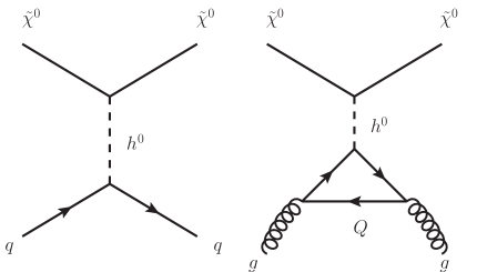
Figure 1: The Higgs-boson exchange processes that contribute at leading order to the spin-independent scattering of wino-like neutralino with nucleons.

The effective four-fermion coupling, $\alpha_{3q}$ in Eq. (5) contains contributions from both squark and Higgs exchange. However, in the region of parameter space of interest here, the squark masses and the heavy Higgs scalar mass, $m_{H}$, are significantly larger than the light Higgs scalar mass, $m_{h}$. Thus, at leading order, wino-like neutralino dark matter-nucleon scattering is induced by the light Higgs-boson exchange processes shown in Fig. 1. By integrating out the Higgs boson, we can readily obtain the effective quark couplings $\alpha_{3q}$ [8, 25]

$$\alpha_{3q}^{(\text{tree})}\simeq\frac{gm_{q}}{4m_{W}m_{h}^{2}}\text{Re}\left[\left(Z_{\chi 3}\cos\beta-Z_{\chi 4}\sin\beta\right)\left(gZ_{\chi 2}-g^{\prime}Z_{\chi 1}\right)\right]~{},$$ (7)

where $g$ and $g^{\prime}$ denote the SU(2)_L and U(1)_Y gauge couplings, respectively, $m_{W}$ is the $W$-boson mass, the $m_{q}$ are the quark masses, and $\tan\beta$ is the ratio of the Higgs VEVs defined by $\tan\beta\equiv\langle H_{u}^{0}\rangle/\langle H_{d}^{0}\rangle$. Note that in the assumed limit, $m_{H}\gg m_{h}\simeq 125$ GeV, the Higgs mixing angle, $\alpha$ can be approximated by the decoupling limit $\alpha\to\beta-\pi/2$, so that $\cos\alpha\to\sin\beta$ and $\sin\alpha\to-\cos\beta$. The $Z_{\chi i}$ ($i=1,2,3,4$) in Eq. (7) are defined by

$$\tilde{\chi}^{0}=Z_{\chi 1}\tilde{B}+Z_{\chi 2}\tilde{W}^{0}+Z_{\chi 3}\tilde{H}_{d}^{0}+Z_{\chi 4}\tilde{H}^{0}_{u}~{},$$ (8)

where $\tilde{B}$, $\tilde{W}^{0}$, $\tilde{H}^{0}_{d}$, and $\tilde{H}^{0}_{u}$, denote the bino, wino, and Higgsino fields, respectively. Focusing on the region of parameter space in which $\tilde{\chi}^{0}$ is wino-like and $m_{W}\ll|M_{i}-\mu|$ ($i=1,2$), where $M_{1}$, $M_{2}$ and $\mu$ are the bino mass, wino mass and Higgsino mixing parameters, respectively, we have

$$Z_{\chi 1}\simeq 0,\quad Z_{\chi 2}\simeq 1, Z_{\chi 3}\simeq\frac{m_{W}}{M_{2}^{2}-\mu^{2}}(M_{2}\cos\beta+\mu\sin\beta),$$

$$Z_{\chi 4} \simeq -\frac{m_{W}}{M_{2}^{2}-\mu^{2}}(M_{2}\sin\beta+\mu\cos\beta)\,,$$ (9)

and we can further approximate Eq. (7) as

$$\alpha_{3q}^{(\text{tree})}\simeq\frac{g^{2}m_{q}(M_{2}+\mu\sin 2\beta)}{4m_{h}^{2}(M_{2}^{2}-\mu^{2})}~{}.$$ (10)

From this expression, we see that $\alpha_{3q}^{(\text{tree})}$ decreases as $\propto\mu^{-1}$ when $|\mu|\gg M_{2}$, which is the case for the AMSB so long as $m_{0}\ll m_{3/2}$. These approximations also hold in the PGM model for values of $\tan\beta$ that maintain $|\mu|\gg M_{2}$.

The contribution of the diagrams in Fig. 1 to the effective nucleon couplings is obtained by using the nucleon matrix elements of the quark-antiquark scalar operators, $\bar{q}q$. Their values are often described by the mass fractions $f_{T_{q}}^{(N)}$ defined by

$$m_{N}f_{T_{q}}^{(N)}\equiv\langle N|m_{q}\bar{q}q|N\rangle\equiv\sigma_{q}\equiv m_{q}B_{q}^{N}\,,$$ (11)

with $m_{N}$ the nucleon mass. For the light quarks, combinations of the matrix elements can be related to $\sigma$ terms such as the pion-nucleon $\sigma$ term

$$\Sigma_{\pi N}\;=\;\frac{1}{2}(m_{u}+m_{d})\left(B_{u}^{p}+B_{d}^{p}\right)\,,$$ (12)

which may be computed directly with lattice simulations [29] or extracted phenomenologically from data on low-energy $\pi$-nucleon scattering or on pionic atoms [30]. Another combination can be extracted phenomenologically from the octet baryon mass splittings,

$$\sigma_{0}\;=\;\frac{1}{2}(m_{u}+m_{d})\left(B_{u}^{p}+B_{d}^{p}-2B_{s}^{p}\right)\,,$$ (13)

which gives

$$\sigma_{s}=m_{s}B^{p}_{s}=\frac{m_{s}}{m_{u}+m_{d}}(\Sigma_{\pi N}-\sigma_{0})\,.$$ (14)

A third relation is obtained from baryon octet masses

$$z\;\equiv\;\frac{B_{u}^{p}-B_{s}^{p}}{B_{d}^{p}-B_{s}^{p}}\;=\;\frac{m_{\Xi^{0}}+m_{\Xi^{-}}-m_{p}-m_{n}}{m_{\Sigma^{+}}+m_{\Sigma^{-}}-m_{p}-m_{n}}\;=\;1.49\,.$$ (15)

From a recent compilation in Ref. [31], we use

$$\Sigma_{\pi N}\;=\;46\pm 11\;{\rm MeV}\qquad\sigma_{s}\;=\;35\pm 16\;{\rm MeV}\,,$$ (16)

which determines the matrix elements of the three light quarks and we list them in the first three columns of Table 1 for the reader’s convenience.

Table 1: Values of the mass fractions $f^{(N)}_{T_{q,G}}$ obtained in Ref. [31].

	$f^{(N)}_{T_{u}}$	$f^{(N)}_{T_{d}}$	$f^{(N)}_{T_{s}}$	$f^{(N)}_{T_{G}}$	$f^{(N)}_{T_{c}}$	$f^{(N)}_{T_{b}}$	$f^{(N)}_{T_{t}}$
Proton	0.018(5)	0.027(7)	0.037(17)	0.917(19)	0.078(2)	0.072(2)	0.069(1)
Neutron	0.013(3)	0.040(10)	0.037(17)	0.910(20)	0.078(2)	0.071(2)	0.068(2)

The contributions of the heavy quarks to the scattering cross section are often calculated by integrating them out and replacing them by the one-loop gluon contributions so that $f_{T_{Q}}^{(N)}=\frac{2}{27}f_{T_{G}}^{(N)}$ for $Q=c,b,t$, where the nucleon matrix element of the gluon scalar operator is evaluated using the trace anomaly formula given in [32]:

$$\langle N|\frac{\alpha_{s}}{\pi}G^{a}_{\mu\nu}G^{a\mu\nu}|N\rangle=-\frac{8}{9}m_{N}f_{T_{G}}^{(N)}~{},$$ (17)

which holds at the leading order in $\alpha_{s}$, and we note in addition that $f_{T_{G}}^{(N)}\equiv 1-\sum_{q=u,d,s}f_{T_{q}}^{(N)}$.

However, momenta around the mass scale of the quark running in the loop make the most important contributions to the integral in the loop diagram shown in Fig. 1. These contributions are often referred to as long-distance contributions as the relevant energy scales are much lower than the electroweak scale in the cases of the charm and bottom quarks. Since $\alpha_{s}(m_{Q})$ is rather large at the scales of these masses, higher-order QCD corrections are significant. We take these corrections into account to ${\cal O}(\alpha_{s}^{3})$ in perturbative QCD, following Ref. [33], finding

$$\sigma_{c} = \frac{2}{27}\left(-0.3+1.48f^{(N)}_{T_{G}}\right)M_{N}\;=\;73.4\pm 1.9\;{\rm MeV}\,,$$ (18)

$$\sigma_{b} = \frac{2}{27}\left(-0.16+1.23f^{(N)}_{T_{G}}\right)M_{N}\;=\;67.3\pm 1.6\;{\rm MeV}\,,$$ (19)

$$\sigma_{t} = \frac{2}{27}\left(-0.05+1.07f^{(N)}_{T_{G}}\right)M_{N}\;=\;64.7\pm 1.4\;{\rm MeV}\,.$$ (20)

Using (11), the corrected contributions for all quarks can then be expressed in terms of the effective mass fractions $f^{(N)}_{T_{Q}}$, whose values we show in the last three columns of Table 1. The resulting effective coupling is given by

$$f_{N}^{(\text{tree})}=m_{N}\sum_{q=u,d,s,c,b,t}\frac{\alpha_{3q}^{(\text{tree})}}{m_{q}}f_{T_{q}}^{(N)}~{}.$$ (21)

This treatment increases the resulting value of $f_{N}$ by ${\cal O}(10)$% [31] relative to computing $f_{N}$ using a common $f_{T_{Q}}^{(N)}$ for the heavy quarks. We note that even though the contributions from heavy quarks are induced by QCD loop diagrams, the resultant contributions are similar in magnitude to those from the light quarks [23, 26, 27]. This is because of the large contribution of the gluons to the mass of nucleon: $f_{T_{G}}^{(N)}\gg f_{T_{q}}^{(N)}$.

2.3 Electroweak loop contributions

As seen in Eq. (10), the tree-level Higgs exchange contribution is suppressed when the Higgsino mass is very large. In this case, the contributions from the loop processes shown in Figs. 2 and 3 may dominate over the tree-level contribution [34]. These loop contributions have been computed in the literature [26, 27, 35, 36, 37], and we include them in our analysis with the following approximations:

• We use the results obtained for a pure wino, though the wino-like neutralino LSP in our case also contains admixtures of the bino and Higgsinos. This approximation is valid since the loop corrections can be significant only when the Higgsino mass is quite large so that the tree-level bino contribution becomes small—in this case, $|Z_{\chi 1}|,|Z_{\chi 3}|,|Z_{\chi 4}|\ll 1$ as can be seen from Eq. (9), i.e., the LSP is almost pure wino.

• Although the electroweak loop contributions have been computed at NLO in QCD [37], we use the LO result, since the difference between the two approximations can be neglected for our purposes.

In the rest of this subsection, we summarize our results for the electroweak loop contributions.

The left diagram in Fig. 2 gives rise to scalar light-quark operators, with coefficients given by

$$\alpha_{3q}^{(\text{loop})}=\frac{\alpha_{2}^{2}m_{q}}{4m_{W}m_{h}^{2}}g_{\rm H}(\omega)~{},$$ (22)

where $\alpha_{2}\equiv g^{2}/(4\pi)$ is the SU(2)_L coupling strength and $\omega\equiv m_{W}^{2}/m_{\chi}^{2}$. The mass function $g_{\text{H}}(x)$ is given in the Appendix. In addition, heavy quarks provide scalar gluon operator contributions via the two-loop diagrams in Fig. 3. As in the case of the tree-level Higgs exchange processes, these two-loop contributions can be comparable to the one-loop contribution to the scalar quark operators, even though they are induced at a higher order in ${\cal O}(\alpha_{s})$.

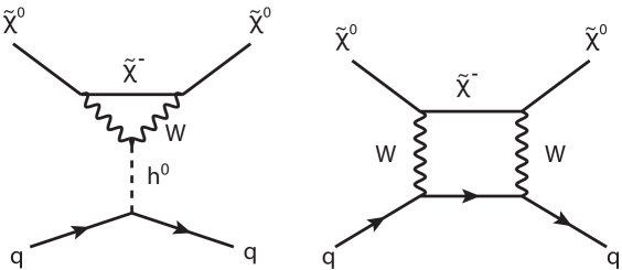
Figure 2: One-loop contributions to wino-nucleon scattering.

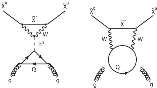
Figure 3: Two-loop contributions to wino-nucleon scattering.

We again take account of the long-distance QCD corrections to the left diagram in Fig. 3 by using the $f^{(N)}_{T_{Q}}$ $(Q=c,b,t)$ values given in Table 1. For each heavy quark we have

$$\alpha_{3Q}^{(\text{loop})}=\frac{\alpha_{2}^{2}m_{Q}}{4m_{W}m_{h}^{2}}g_{\rm H}(\omega)~{},$$ (23)

which is the same as in Eq. (22).

The contribution from the right diagram in Fig. 3 is included in the coefficient $\alpha_{G}$ of the scalar gluon operator:

$$\alpha_{G}=2\times\frac{\alpha_{2}^{2}}{4m_{W}^{3}}g_{\rm B1}(\omega)+\frac{\alpha_{2}^{2}}{4m_{W}^{3}}g_{\rm B3}(\omega,\tau)\ ,$$ (24)

where $\tau\equiv m_{t}^{2}/m_{\chi}^{2}$ and the mass functions $g_{\text{B1}}$ and $g_{\text{B3}}$ are given in the Appendix. The first (second) term in the right-hand side of the above expression corresponds to the first- and second-generation (third-generation) contribution. We use the LO formula (17) to evaluate the nucleon matrix element of the gluon scalar operator. A more systematic treatment for the inclusion of the higher-order QCD effects as well as the separation between the long- and short-distance contributions using the matching procedure is discussed in Ref. [37].

The right diagram in Fig. 2 induces interactions described by the twist-2 operators in Eq. (5). The Wilson coefficients of these operators are found to be

$$\beta_{1q} =\frac{\alpha_{2}^{2}}{m_{W}^{3}}g_{\rm T1}(\omega)\ ,$$ (25)

$$\beta_{2q} =\frac{\alpha_{2}^{2}}{m_{W}^{3}}g_{\rm T2}(\omega)\ ,$$ (26)

for $q=u,d,s,c$ and

$$\beta_{1b} =\frac{\alpha_{2}^{2}}{m_{W}^{3}}h_{\rm T1}(\omega,\tau)\ ,$$ (27)

$$\beta_{2b} =\frac{\alpha_{2}^{2}}{m_{W}^{3}}h_{\rm T2}(\omega,\tau)\ ,$$ (28)

for the $b$ quark. The nucleon matrix elements of the twist-2 operators are given by the second moments of the parton distribution functions (PDFs) [23, 24]:

$$\langle N(p)|{\cal O}_{\mu\nu}^{q}|N(p)\rangle =m_{N}\left(\frac{p_{\mu}p_{\nu}}{m_{N}^{2}}-\frac{1}{4}\eta_{\mu\nu}\right)\left[q_{N}(2)+\bar{q}_{N}(2)\right]~{},$$ (29)

with

$$q_{N}(2) =\int^{1}_{0}dx~{}x\ q_{N}(x)~{},$$ (30)

$$\bar{q}_{N}(2) =\int^{1}_{0}dx~{}x\ \bar{q}_{N}(x)~{},$$ (31)

where $q_{N}(x)$ and $\bar{q}_{N}(x)$ are the PDFs of the quark and antiquark, respectively. We present in Table 2 the values of the second moments at the scale $\mu=m_{Z}$ for the proton, where we have used the CJ12 NLO PDFs given by the CTEQ-Jefferson Lab collaboration [38]. As mentioned above, there is also a gluon twist-2 contribution, but this can be neglected, as it is higher order in $\alpha_{s}/\pi$, and the nucleon matrix element of the gluon twist-2 operator, $g(2)$, is not so much larger than the light-quark operators, $u(2)$ and $d(2)$, in contrast to the cases for the scalar operators. Thus the gluon twist-2 contribution is always suppressed by an extra $\alpha_{s}/\pi$ factor compared to the light-quark twist-2 contributions.

Table 2: Second moments of the PDFs of partons in the proton evaluated at $\mu=m_{Z}$. We use the CJ12 next-to-leading order PDFs given by the CTEQ-Jefferson Lab collaboration [38].

$g(2)$	0.464(2)
$u(2)$	0.223(3)	$\bar{u}(2)$	0.036(2)
$d(2)$	0.118(3)	$\bar{d}(2)$	0.037(3)
$s(2)$	0.0258(4)	$\bar{s}(2)$	0.0258(4)
$c(2)$	0.0187(2)	$\bar{c}(2)$	0.0187(2)
$b(2)$	0.0117(1)	$\bar{b}(2)$	0.0117(1)

2.4 Summary

Combining the results above, the effective coupling $f_{N}$ is evaluated as

$$\frac{f_{N}}{m_{N}} =\frac{f_{N}^{(\text{tree})}}{m_{N}}+\sum_{q=u,d,s,c,b,t}f_{T_{q}}^{(N)}\frac{\alpha_{3q}^{(\text{loop})}}{m_{q}}-\frac{8}{9}f_{T_{G}}^{(N)}\alpha_{G}+\sum_{q=u,d,s,c,b}\frac{3}{4}(q_{N}(2)+\bar{q}_{N}(2))(\beta_{1q}+\beta_{2q})~{},$$ (32)

where $f_{N}^{(\text{tree})}$ is given in Eq. (21), the $f_{T_{q}}^{(N)}$ are given in Table 1, $\alpha_{3q}^{(\text{loop})}$ is given in Eq. (22), $\alpha_{G}$ is given in Eq. (24), $\beta_{1q}$ and $\beta_{2q}$ are shown in Eqs. (26) and (28), respectively, the second moments $q_{N}(2)$ and $\bar{q}_{N}(2)$ are given in Table 2, and the mass functions in the coefficients are summarized in the Appendix.

3 Calculation of the Relic Density and Higgs Mass

3.1 Relic Wino LSP Density

As discussed earlier, the mAMSB model is characterized by three continuous parameters, $m_{3/2},m_{0}$ and $\tan\beta$, and the sign of $\mu$. Examples of $(m_{0},m_{3/2})$ planes with $\tan\beta=5$ and 2 and both signs of $\mu$ are shown in Fig. 4, which updates a similar plot given in [4]. In the pink shaded region to the right of each panel, there are no solutions for the minimization of the Higgs potential, and therefore radiative electroweak symmetry breaking is not possible in this region. The red lines are contours of $m_{h}$ in GeV. (Our calculation of the Higgs mass is discussed in more detail below.) In the largely horizontal blue-shaded region the LSP relic density is $\Omega_{\chi}h^{2}=0.12\pm 0.01$.

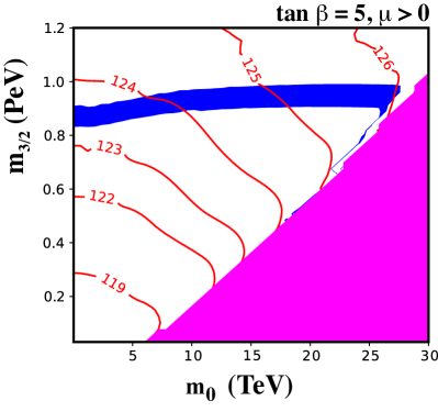
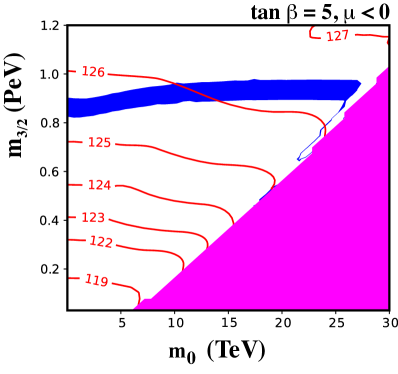
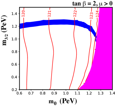
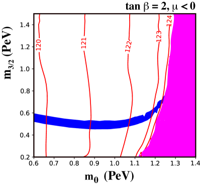
Figure 4: The $(m_{0},m_{3/2})$ plane in the mAMSB/PGM models for $\tan\beta=5$ (upper panels) and $\tan\beta=2$ (lower panels) for $\mu>0$ (left panels) and $\mu<0$ (right panels). Electroweak symmetry breaking does not occur in the region shaded pink. Contours of $m_{h}$ are shown as red lines labeled in units of GeV. The LSP relic density is $\Omega_{\chi}h^{2}=0.12\pm 0.01$ in the region shaded blue.

The wino mass increases monotonically with $m_{3/2}$ as seen in Eq. (2). For $\tan\beta=5$ and $m_{3/2}\approx 0.9-1$ PeV, the wino mass is roughly 3 TeV and, as seen in the upper panels of Fig. 4, it is able to provide the correct relic density when the Sommerfeld enhancements are included. For relatively low values of $\tan\beta$ such as those chosen in Fig. 4, the Higgs mass is quite sensitive to parameter choices and increases with $\tan\beta$, and we find that for $\tan\beta\simeq 5$ the relic density is satisfied for an acceptable value of the Higgs mass.

We note that, as $m_{0}$ increases, the value of the $\mu$ eventually starts to decrease so that the LSP becomes more Higgsino-like close to the region with no electroweak symmetry breaking. When $\mu\sim 1$ TeV and $m_{3/2}$ is sufficiently large the LSP is almost a pure Higgsino and the relic density is acceptable. This region is visible as the diagonal blue strip running close to the boundary of the pink-shaded region in the upper panels of Fig. 4. However, we do not consider this strip, as our approximations for the elastic scattering cross section only apply in the wino-like case represented by the horizontal blue-shaded band .

As one can see in the upper panels of Fig. 4, for $\tan\beta=5$ the requirements of electroweak symmetry breaking and the cold dark matter density enforce $m_{0}\ll m_{3/2}$. PGM boundary conditions with $m_{0}\simeq m_{3/2}$ are only possible at lower values of $\tan\beta\simeq 2$ [6]. In the lower two panels of Fig. 4, we show the $(m_{0},m_{3/2})$ plane with $\tan\beta=2$. In the horizontal blue-shaded region, the LSP is again wino-like with the required relic density. The Higgs mass is generally too low, except for the largest values of $m_{0}$ allowed by radiative electroweak symmetry breaking. We note that higher values of $m_{h}$ can be attained for slightly higher values of $\tan\beta$. For example, $m_{h}=125$ GeV is possible for $\tan\beta=2.05$.

The neutralino mass spectra for $\tan\beta=2$ and 5 are shown in Fig. 5 for both signs of $\mu$. Along each of the curves, the value of $m_{3/2}$ is chosen so that the relic density is $\Omega_{\chi}h^{2}=0.12$. For $\tan\beta=5$, the range of gravitino masses is 0.87–0.95 PeV for $\mu>0$ and 0.86–0.94 PeV for $\mu<0$. Similarly, the range for the gravitino mass when $\tan\beta=2$ is 1.0–1.3 PeV for $\mu>0$ and 0.49–0.70 PeV for $\mu<0$. In all of the cases shown, we see that both the bino and wino masses are relatively independent of $m_{0}$ when $m_{0}\ll m_{3/2}$. On the other hand, the Higgsino mass is quite sensitive to $m_{0}$, as it is essentially determined by $\mu$, which is in turn fixed by the electroweak symmetry breaking conditions. At very large $m_{0}$, $|\mu|$ begins to drop, and at sufficiently large $m_{0}$ the focus-point region [13] is reached and the Higgsino becomes the LSP.

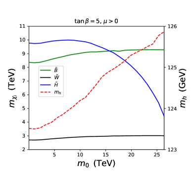
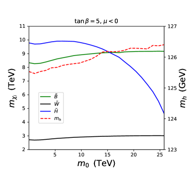
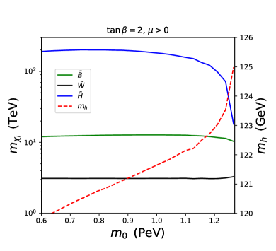
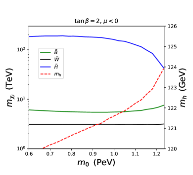
Figure 5: Calculations of the neutralino and Higgs masses as functions of $m_{0}$ for $\tan\beta=5$ (upper panels) and $\tan\beta=2$ (lower panels) and $\mu>0$ (left panels) and $\mu<0$ (right panels). The (Higgsino-) (bino-) wino-like mass contours are (blue) (red) black. For each value of $m_{0}$, the value of $m_{3/2}$ is chosen so that the relic LSP density is $\Omega_{\chi}h^{2}=0.12$. Also shown is the Higgs mass given by the scale on the right.

It is instructive to consider the dependences of the neutralino masses on $\tan\beta$ as shown in the left panels of Fig. 6 for the cases $m_{3/2}=950$ TeV, $m_{0}=15$ TeV and both signs of $\mu$. We see that the lightest neutralino is always wino-like with a mass around 3 TeV, and the bino-like neutralino has a mass $\sim 9$ TeV. The second lightest neutralino is bino-like for $\tan\beta\lesssim 5$ and Higgsino-like for larger $\tan\beta$. Also shown in the left panels of Fig. 6 is the Higgs mass plotted as a function of $\tan\beta$. Here we see clearly the strong dependence of $m_{h}$ on $\tan\beta$ for $\tan\beta\lesssim 10$. All of the masses are relatively independent of $\tan\beta$ when $\tan\beta\gtrsim 10$.

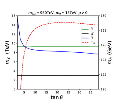
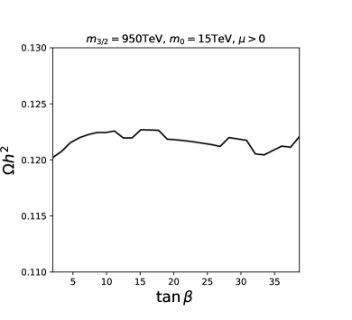
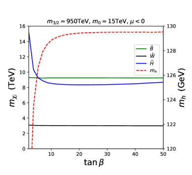
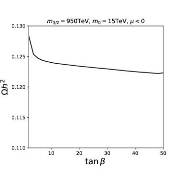
Figure 6: Neutralino and Higgs masses (left panels) and the cold dark matter density (right panels) as functions of $\tan\beta$ for $m_{3/2}=950$ TeV, $m_{0}=15$ TeV with $\mu>0$ (upper panels) and $\mu<0$ (lower panels). The lightest neutralino is always wino-like (black line). The bino-like neutralino mass is shown as a green line and the Higgsino-like neutralino masses as a blue line. (The two Higgsinos are nearly degenerate.) The red dashed line shows the Higgs mass.

For the same choices of parameters, we show the relic LSP density as a function of $\tan\beta$ in the right panels of Fig. 6. While it might appear that there is a strong dependence on $\tan\beta$, this is largely due to the choice of scale. The relic density is acceptable (particularly when calculational uncertainties are taken into account) throughout the range of $\tan\beta$ shown.

In the limit that $m_{0}=m_{3/2}$ as in PGM models, only a relatively narrow range of $\tan\beta$ is allowed, as seen in Figs. 7 where the neutralino and Higgs masses and relic density are plotted as functions of $\tan\beta$ assuming $m_{0}=m_{3/2}=1.15$ PeV for $\mu>0$ (upper panels) and $m_{0}=m_{3/2}=0.7$ PeV for $\mu<0$ (lower panels). The mass spectra plotted in the left panels show again a wino-like LSP with mass around 3 TeV. Because the $\mu$ parameter typically takes values of order $m_{0}$, the Higgsino masses are very large in this case until $\tan\beta$ is sufficiently large that the focus-point region is approached. At this point, the Higgs mass is increased toward its experimental value. At still larger $\tan\beta$ radiative electroweak symmetry breaking is no longer possible.

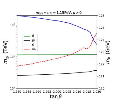
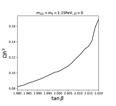
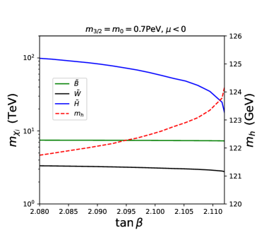
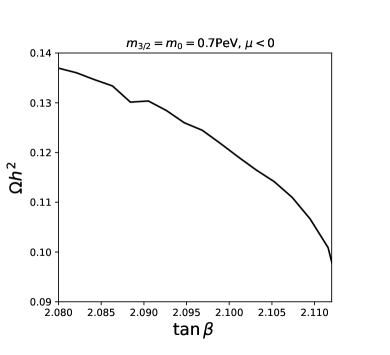
Figure 7: Neutralino and Higgs masses (left panels) and the relic LSP density (right panels) as functions of $\tan\beta$ for the PGM model when $m_{3/2}=m_{0}=1.15$ PeV with $\mu>0$ (upper panels) and $\mu<0$ (lower panels).

The relic LSP density for the same sets of parameters is shown in right panels of Fig. 7. Depending on the sign of $\mu$, the relic LSP density (which is always close to the observationally determined values) increases ($\mu>0$) or decreases ($\mu<0$), tracking the behavior of the wino-like LSP mass.

3.2 Calculation of the Higgs Boson Mass

Reliable calculations of the light Higgs mass are challenging when the supersymmetry-breaking scale is ${\cal O}({\rm PeV})$, as is the case for the AMSB and PGM models considered here. Accordingly, we have compared results from two codes: FeynHiggs 2.18.1 [40] and mhsplit, a simplified code devised specifically for large supersymmetry-breaking scales. Following [41, 42], the 2-loop RGE evolution of the couplings of the effective theory below the supersymmetry breaking scale are used to obtain the Higgs mass at full next-to-leading order accuracy as described in more detail in [43] for a model with an AMSB-like spectrum. The same code was also adapted to PGM models [6]. A comparison of the results of the two codes is shown in Fig. 8, where we plot the Higgs mass as a function of $m_{0}$ given by each code for $m_{3/2}=950$ TeV and $\tan\beta=2$ with $\mu>0$ (left) and $\mu<0$ (right). The Higgs mass from mhsplit is shown by the (smooth) solid curve, and that from FeynHiggs 2.18.1 by the dashed curve. For $m_{0}=0.1-0.6$ PeV, both codes are in good agreement and appear well-behaved. At lower values of $m_{0}$, the approximations used in mhsplit break down. At $m_{0}\gtrsim 0.6$ PeV, FeynHiggs 2.18.1 starts to exhibit irregularities that are absent in the simplified calculation.

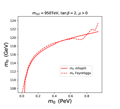
(a) $\mu>0$

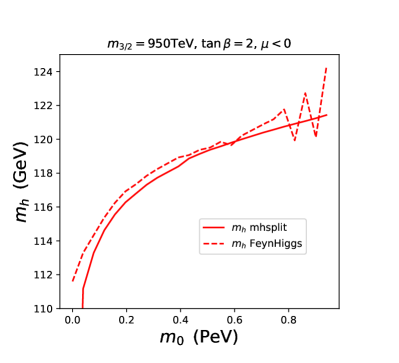
(b) $\mu<0$

Figure 8: Comparisons of the calculations of $m_{h}$ made using FeynHiggs 2.18.1 (dashed lines) and mhsplit, a simplified code devised specifically for large supersymmetry-breaking scales (solid lines). We see that the simplified calculation of $m_{h}$ is very stable at large values of $m_{0}$ for $m_{3/2}=950$ TeV, $\tan\beta=2$ and both signs of $\mu$, and agrees very well with the FeynHiggs results for values of $m_{0}\simeq 0.1-0.6$ PeV.

Motivated by the above comparison, the Higgs mass contours for the mAMSB models shown in the upper panels of Fig. 4 are run using FeynHiggs 2.18.1, whereas those in the lower panels for the PGM-like models with significantly higher supersymmetry-breaking mass parameters are run using mhsplit. The Higgs mass as a function of $m_{0}$ for fixed $\tan\beta$ and $m_{3/2}$ fixed to yield $\Omega_{\chi}h^{2}=0.12$ is shown in Fig. 5. The upper panels with $\tan\beta=5$ are calculated using FeynHiggs 2.18.1 while the lower panels with $\tan\beta=2$ are calculated using mhsplit. As one can see, the scalar mass range there is highly sensitive to $\tan\beta$. It is relatively easy in the mAMSB models with $\tan\beta=5$ to obtain acceptable Higgs masses with $m_{0}\sim\mathcal{O}(10)$ TeV, whereas $m_{0}\gtrsim 1$ PeV is required in the PGM model with $\tan\beta=2$, and an acceptable Higgs mass is only possible when the Higgsino mass drops precipitously as one approaches the focus-point region. The dependence of the Higgs mass on $\tan\beta$ is shown in Fig. 6 for the mAMSB models and in the left panels of Fig. 7 for the PGM models.

4 Results for the Spin-Independent Wino Scattering Cross Section

We now present our results for the spin-independent scattering cross section of a wino-like neutralino, $\sigma_{p}$, obtained using the results presented in Section 2. Explicit expressions for the mass functions introduced there are given in the Appendix. We also provide in the Appendix simple approximate formulae that apply when the wino-like neutralino mass $m_{\chi}$ is much larger than the electroweak scale, which is the case for the parameter regions of interest in this paper.

We present in Fig. 9 a comparison of calculations of $\sigma_{p}$ made using tree-level matrix elements (solid black lines) and one-loop calculations (solid blue lines). The spin-independent cross section is plotted as a function of $m_{0}$ for the AMSB model with $\tan\beta=5$ (upper panels) for both $\mu>0$ (left panels) and $\mu<0$ (right panels). In the lower panels we show the cross section in the PGM-like model with $\tan\beta=2$. The orange-shaded region in each plot corresponds to cross sections in the neutrino fog [17]. For comparison, we note that for $m_{\chi}\simeq 3$ TeV the current best experimental limit, from the LUX-ZEPLIN (LZ) experiment [44], is $\sigma_{p}\lesssim 10^{-9}$ pb.

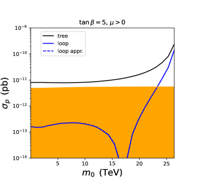
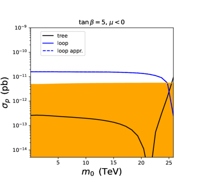
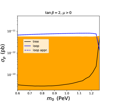
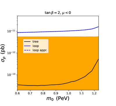
Figure 9: Comparison of calculations of $\sigma_{p}$ as a function of $m_{0}$ made using tree-level matrix elements (black lines) and one-loop calculations made using the full expressions in the Appendix (solid blue lines) and the simplified expressions in Eq. (42) that become exact when the wino neutralino mass $m_{\chi}\gg m_{W}$ (dashed blue lines). The calculations are for the AMSB model with $m_{3/2}=950$ TeV, $m_{0}=15$ TeV and both signs of $\mu$ (upper panels) and the PGM-like model with $m_{3/2}=m_{0}=1.15$ PeV for $\mu>0$ (lower left panel) and with $m_{3/2}=m_{0}=0.7$ PeV for $\mu<0$ (lower left panel). The orange-shaded region corresponds to cross section values in the neutrino fog.

In the mAMSB model with $\tan\beta=5$ and $\mu>0$, we have the discouraging result that although the tree level result is above the neutrino fog (and hence in principle observable, though it is still two orders of magnitude below the current LZ limit), the one-loop correction induces a cancellation and the cross section drops into the neutrino fog unless $m_{0}\gtrsim 23$ TeV. Indeed, the cancellation is near-total when $m_{0}=16$ TeV. This cancellation can be understood by looking at the tree and loop contributions to the cross section separately. From Eqs. (10) and (21), we see that $\alpha_{3q}/m_{q}$ is independent of $m_{q}$ for a wino LSP in mAMSB, and we can write

$$f_{p}^{(\rm tree)}\simeq 2\times 10^{-6}{\rm GeV}^{-1}\times\frac{(M_{2}+\mu\sin 2\beta)}{(M_{2}^{2}-\mu^{2})}\,,$$ (33)

when taking $m_{h}=125$ GeV. When the relic density is fixed, requiring the wino mass, $M_{2}\simeq 3$ TeV, and noting that $\mu$ (nearly equal to the Higgsino mass shown in Fig. 5) varies with $m_{0}$, we see that the tree-level cross section varies little at low $m_{0}$ (as does $\mu$) and increases as $\mu$ begins to drop. This is the behaviour seen in the upper left panel of Fig. 9. When $M_{2}\simeq 3$ TeV for wino DM and $m_{h}$ is restricted to the observed value, the loop correction is roughly constant and takes the value

$$f_{p}^{(\rm loop)}\simeq 1.6\times 10^{-10}\,{\rm GeV}^{-2}\,.$$ (34)

However, when $\mu>0$ the tree level amplitude is negative and for a certain value of $\mu$ ($m_{0}$) will cancel the one-loop contribution as seen in Fig. 9. It is easy to see that a complete cancellation, $f_{p}^{(\rm tree)}+f_{p}^{(\rm loop)}=0$, occurs when

$$\sin 2\beta\simeq\frac{\mu}{12{\rm TeV}}-\frac{3.7{\rm TeV}}{\mu}\,.$$ (35)

This occurs when $m_{0}\sim 17$ TeV, when $\tan\beta=5$ and $\mu\sim 9$ TeV as seen in Fig. 5. However, we note that the amplitude will not vanish if $|\mu|\gtrsim 15$ TeV. This same cancellation can be seen in the upper panels of Fig. 10, where we show the cross section as a function of $\tan\beta$ for $m_{3/2}=950$ TeV and $m_{0}=15$ TeV. 

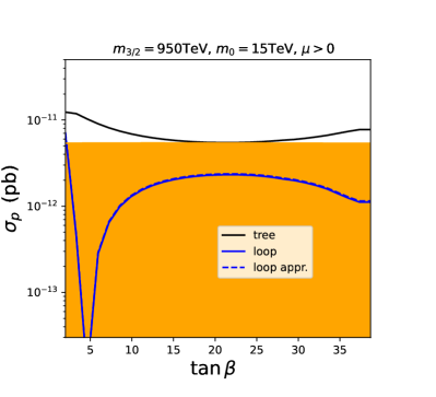
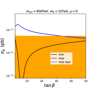
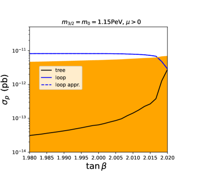
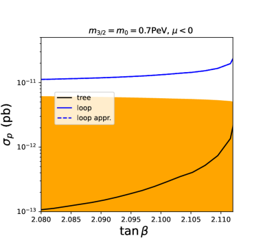
Figure 10: Comparison of calculations of $\sigma_{p}$ as a function of $\tan\beta$ made using tree-level matrix elements (black lines) and one-loop calculations made using the full expressions in the Appendix (solid blue lines) and the simplified expressions in Eq. (42) that become exact when the wino neutralino mass $m_{\chi}\gg m_{W}$ (dashed blue lines). The calculations are for the AMSB model with $m_{3/2}=950$ TeV, $m_{0}=15$ TeV and both signs of $\mu$ (upper panels) and the PGM-like models with $m_{3/2}=m_{0}=1.15$ PeV for $\mu>0$ (lower left panel) and with $m_{3/2}=m_{0}=0.7$ PeV for $\mu<0$ (lower right panel). The orange-shaded region corresponds to cross sections in the neutrino fog. In all four panels the value of $m_{3/2}$ is chosen to give $\Omega h^{2}\simeq 0.12$.

On the other hand, the tree-level scattering amplitude vanishes when $M_{2}+\mu\sin 2\beta=0$. For $\tan\beta=5$, this occurs when $\mu\sim-8$ TeV, corresponding to $m_{0}\sim 21$ TeV. However, when $\mu<0$ the one-loop correction can enhances the total cross section, lifting it out of the neutrino fog and into the domain of possible experimental observation (though still unobservable at present). The large loop correction can significantly shift this point of vanishing amplitude. In the case of the upper right panel of Fig. 9, the cancellation would occur at $m_{0}>25$ TeV, past the point where radiative electroweak symmetry breaking is possible.

In the PGM-like model with $\tan\beta=2$ ($\sin 2\beta=0.8$), $\mu\gg M_{2}$, and the tree-level amplitude is approximately proportional to $1/\mu$. So long as $\mu$ is very large, the one-loop correction dominates the cross section substantially, lifting it out the neutrino fog unless $m_{0}\gtrsim 1.2$ PeV when $\mu>0$, as seen in the lower panels of Figs. 9 and 10.

Before concluding, we note that the tree-level cross section in the mAMSB model was explored in a frequentist analysis using constraints from cosmology and accelerator experiments in [3]. The best-fit cross section for wino dark matter was found to be slightly above (below) the neutrino fog for $\mu>0$ ($\mu<0$), and values for $\mu<0$ extended far into the neutrino fog. It was also found that values of the cross section extend to much higher values. This occurs when $m_{0}$ takes large values and approaches the region with no electroweak symmetry breaking. This behaviour is seen, for example, in the upper left panel of Fig. 9 where the cross section increases by over an order of magnitude as $m_{0}$ is increased.

5 Conclusion and Discussion

The results in Figs. 9 and 10 illustrate clearly the potential importance of one-loop electroweak corrections to the spin-independent scattering cross section for a wino-like LSP. In the case of the AMSB model, the results in the upper panels of these two figures show sharp difference between the two signs of $\mu$. In the case of positive $\mu$ (upper left panels), the one-loop correction interferes negatively with the tree-level contribution and has similar magnitude, potentially causing a total cancellation. On the other hand, in the case of negative $\mu$ (upper right panels), the one-loop correction has the same sign as the tree-level contribution for $m_{0}\lesssim 20$ TeV and $\tan\beta\lesssim 5$, enhancing the spin-independent scattering cross section. Furthermore, in the case of the PGM-like model shown in the lower panels of Figs. 9 and 10, the one-loop corrections enhance the cross section for both signs of $\mu$.

The consequences of these effects is to invert the conclusions about experimental observability that would be drawn from considering naively the tree-level cross section alone. In the case of the AMSB model shown in the upper panels of Figs. 9 and 10, whereas the tree-level calculation gives an observable cross section for $\mu>0$ and a cross section lost in the neutrino fog for $\mu<0$, the one-loop correction pushes the cross section down into the fog for most values of $m_{0}$ and $\tan\beta$ when $\mu>0$ and lifts it out of the fog when $\mu<0$. On the other hand, in the PGM-like model shown in the lower panels of Figs. 9 and 10, the effect of the one-loop electroweak correction is generally positive, lifting the spin-independent cross section out of the fog for most of the displayed ranges of $m_{0}$ and $\tan\beta$.

The one-loop electroweak corrections must therefore be taken into account when assessing the implications of direct searches for the scattering of cold dark matter on nuclear targets for the viability of AMSB and PGM-like models.  The good news is that the cross section is likely to be above the neutrino fog for the AMSB model if $\mu<0$ and for PGM-like models with either sign of $\mu$. On the other hand, even in these encouraging cases the cross section is not much higher than the neutrino fog, so a strenuous experimental effort [45] will be necessary to explore these models. However, the results of this paper indicate that this effort would have a good chance of being rewarded if it is able to reach down to the level of the neutrino fog.

Appendix

We list here explicit expressions for the mass functions introduced above:

$$g_{\rm H}(x) =2\sqrt{x}(2-x\ln x)-\frac{2}{b_{x}}(2+2x-x^{2})\tan^{-1}\biggl{(}\frac{2b_{x}}{\sqrt{x}}\biggr{)}~{},$$ (36)

$$g_{\rm B1}(x) =\frac{1}{24}\sqrt{x}(2-x\ln x)+\frac{1}{24b_{x}}(4-2x+x^{2}){\rm tan}^{-1}\biggl{(}\frac{2b_{x}}{\sqrt{x}}\biggr{)}~{},$$ (37)

$$g_{\rm B3}(x,y) =-\frac{x^{\frac{3}{2}}(2y-x)}{12(y-x)^{2}}-\frac{x^{\frac{3}{2}}y^{3}\ln y}{24(y-x)^{3}}+\frac{x^{\frac{5}{2}}(3y^{2}-3xy+x^{2})\ln x}{24(y-x)^{3}}$$

$$+\frac{x^{\frac{3}{2}}\sqrt{y}(y^{3}-2y^{2}-14y+6x)\tan^{-1}\left(\frac{2b_{y}}{\sqrt{y}}\right)}{24b_{y}(y-x)^{3}}$$

$$-\frac{x\left(x^{4}-3yx^{3}-2x^{3}+3y^{2}x^{2}+6yx^{2}+4x^{2}-6y^{2}x-6yx-6y^{2}\right)\tan^{-1}\left(\frac{2b_{x}}{\sqrt{x}}\right)}{24b_{x}(y-x)^{3}}\ ,$$

$$g_{\rm T_{1}}(x) =\frac{1}{12}\sqrt{x}\{1-2x-x(2-x)\ln x\}+\frac{1}{3}b_{x}(2+x^{2})\tan^{-1}\biggl{(}\frac{2b_{x}}{\sqrt{x}}\biggr{)}~{},$$ (38)

$$g_{\rm T_{2}}(x) =-\frac{1}{4}\sqrt{x}\{1-2x-x(2-x)\ln x\}+\frac{1}{4b_{x}}x(2-4x+x^{2})\tan^{-1}\biggl{(}\frac{2b_{x}}{\sqrt{x}}\biggr{)}~{},$$ (39)

$$h_{{\rm T_{1}}}(x,y) =\frac{x^{\frac{3}{2}}\{x(1-2x)+y(13+2x)-2y^{2}\}}{12(x-y)^{2}}$$

$$-\frac{x^{\frac{3}{2}}\{x^{3}(2-x)+2xy(3-3x+x^{2})+6y^{2}(2-x)\}}{12(x-y)^{3}}\ln x$$

$$+\frac{x^{\frac{3}{2}}y\{2x(3-6y+y^{2})+y(12+2y-y^{2})\}}{12(x-y)^{3}}\ln y$$

$$+\frac{x\{4x^{2}b_{x}^{2}(2+x^{2})-2xy(6-7x+5x^{2}-x^{3})-6y^{2}(2-4x+x^{2})\}}{12b_{x}(x-y)^{3}}\tan^{-1}\left(\frac{2b_{x}}{\sqrt{x}}\right)$$

$$-\frac{x^{\frac{3}{2}}y^{\frac{1}{2}}\{2x(3-y)(2+5y-y^{2})-y(2-y)(14+2y-y^{2})\}}{12b_{y}(x-y)^{3}}\tan^{-1}\left(\frac{2b_{y}}{\sqrt{y}}\right),$$ (40)

$$h_{{\rm T_{2}}}(x,y) =\frac{x^{\frac{3}{2}}\{x(-1+2x)-(1+2x)y+2y^{2}\}}{4(x-y)^{2}}$$

$$+\frac{x^{\frac{5}{2}}\{(2-x)x^{2}+2y(1-3x+x^{2})\}}{4(x-y)^{3}}\ln x$$

$$+\frac{x^{\frac{3}{2}}y\{y^{2}(y-2)-2x(1-3y+y^{2})\}}{4(x-y)^{3}}\ln y$$

$$+\frac{x^{3}\{x(2-4x+x^{2})-2y(5-5x+x^{2})\}}{4b_{x}(x-y)^{3}}\tan^{-1}\left(\frac{2b_{x}}{\sqrt{x}}\right)$$

$$+\frac{x^{\frac{3}{2}}y^{\frac{3}{2}}(2x(5-5y+y^{2})-y(2-4y+y^{2}))}{4b_{y}(x-y)^{3}}\tan^{-1}\left(\frac{2b_{y}}{\sqrt{y}}\right)~{},$$ (41)

where we have defined $b_{x}\equiv\sqrt{1-x/4}$.

When the mass of the wino-like neutralino $m_{\chi}$ is much larger than the electroweak scale; i.e., $\omega,\tau\to 0$, the above mass functions can be approximated as

$$g_{\rm H}(\omega) \simeq-2\pi\ ,$$

$$g_{\rm B1}(\omega) \simeq\frac{\pi}{12}\ ,$$

$$g_{\rm B3}(\omega,\tau) \simeq\frac{\pi(2+3r)}{24(1+r)^{3}}~{},$$

$$g_{\rm T1}(\omega) \simeq\frac{\pi}{3}\ ,$$

$$g_{\rm T2}(\omega) \simeq 0\ ,$$

$$h_{\rm T1}(\omega,\tau) \simeq\frac{\pi(2+3r)}{6(1+r)^{3}}~{},$$

$$h_{\rm T2}(\omega,\tau) \simeq 0\ ,$$ (42)

with $r\equiv\sqrt{\tau/\omega}=m_{t}/m_{W}$.

References

- [1] M. Dine and D. MacIntire, Phys. Rev. D 46, 2594 (1992) [hep-ph/9205227]; L. Randall and R. Sundrum, Nucl. Phys. B 557, 79 (1999) [arXiv:hep-th/9810155]; G. F. Giudice, M. A. Luty, H. Murayama and R. Rattazzi, JHEP 9812, 027 (1998) [arXiv:hep-ph/9810442]; A. Pomarol and R. Rattazzi, JHEP 9905, 013 (1999) [hep-ph/9903448]; J. A. Bagger, T. Moroi and E. Poppitz, JHEP 0004, 009 (2000) [arXiv:hep-th/9911029]; P. Binetruy, M. K. Gaillard and B. D. Nelson, Nucl. Phys. B 604, 32 (2001) [arXiv:hep-ph/0011081].
- [2] T. Gherghetta, G. Giudice and J. Wells, Nucl. Phys. B 559 (1999) 27 [arXiv:hep-ph/9904378]; E. Katz, Y. Shadmi and Y. Shirman, JHEP 9908, 015 (1999) [hep-ph/9906296]; Z. Chacko, M. A. Luty, I. Maksymyk and E. Ponton, JHEP 0004, 001 (2000) [hep-ph/9905390]; J. L. Feng and T. Moroi, Phys. Rev. D 61, 095004 (2000) [hep-ph/9907319]; G. D. Kribs, Phys. Rev. D 62, 015008 (2000) [hep-ph/9909376]; U. Chattopadhyay, D. K. Ghosh and S. Roy, Phys. Rev. D 62, 115001 (2000) [hep-ph/0006049]; I. Jack and D. R. T. Jones, Phys. Lett. B 491, 151 (2000) [hep-ph/0006116]; H. Baer, J. K. Mizukoshi and X. Tata, Phys. Lett. B 488, 367 (2000) [hep-ph/0007073]; A. Datta, A. Kundu and A. Samanta, Phys. Rev. D 64, 095016 (2001) [hep-ph/0101034]; H. Baer, R. Dermisek, S. Rajagopalan and H. Summy, JCAP 1007, 014 (2010) [arXiv:1004.3297 [hep-ph]]; A. Arbey, A. Deandrea and A. Tarhini, JHEP 1105, 078 (2011) [arXiv:1103.3244 [hep-ph]]; B. C. Allanach, T. J. Khoo and K. Sakurai, JHEP 1111, 132 (2011) [arXiv:1110.1119 [hep-ph]]; A. Arbey, A. Deandrea, F. Mahmoudi and A. Tarhini, Phys. Rev. D 87, no. 11, 115020 (2013) [arXiv:1304.0381 [hep-ph]].
- [3] E. Bagnaschi et al., Eur. Phys. J. C 77 (2017) no.4, 268 [arXiv:1612.05210 [hep-ph]].
- [4] E. Bagnaschi, H. Bahl, J. Ellis, J. Evans, T. Hahn, S. Heinemeyer, W. Hollik, K. A. Olive, S. Paßehr and H. Rzehak, et al. Eur. Phys. J. C 79 (2019) no.2, 149 [arXiv:1810.10905 [hep-ph]].
- [5] M. Ibe, T. Moroi and T. T. Yanagida, Phys. Lett. B 644, 355 (2007) [hep-ph/0610277].
- [6] J. L. Evans, M. Ibe, K. A. Olive and T. T. Yanagida, Eur. Phys. J. C 73, 2468 (2013) [arXiv:1302.5346 [hep-ph]]; J. L. Evans, N. Nagata and K. A. Olive, Phys. Rev. D 91, 055027 (2015) [arXiv:1502.00034 [hep-ph]]; J. L. Evans, N. Nagata and K. A. Olive, Eur. Phys. J. C 79 (2019) no.6, 490 [arXiv:1902.09084 [hep-ph]].
- [7] J. L. Evans, M. Ibe, K. A. Olive and T. T. Yanagida, Phys. Rev. D 91 (2015), 055008 [arXiv:1412.3403 [hep-ph]]; J. L. Evans and K. A. Olive, Phys. Rev. D 106 (2022) no.5, 055026 [arXiv:2202.07830 [hep-ph]].
- [8] T. Falk, A. Ferstl and K. A. Olive, Phys. Rev. D 59, 055009 (1999) [Phys. Rev. D 60, 119904 (1999)] [hep-ph/9806413]; T. Falk, A. Ferstl and K. A. Olive, Astropart. Phys. 13, 301 (2000) [hep-ph/9908311]; J. R. Ellis, A. Ferstl and K. A. Olive, Phys. Lett. B 481, 304 (2000) [hep-ph/0001005]; J. R. Ellis, K. A. Olive, Y. Santoso and V. C. Spanos, Phys. Rev. D 71, 095007 (2005) [hep-ph/0502001].
- [9] V. Mandic, A. Pierce, P. Gondolo and H. Murayama, hep-ph/0008022; J. R. Ellis, J. L. Feng, A. Ferstl, K. T. Matchev and K. A. Olive, Eur. Phys. J. C 24, 311 (2002) [astro-ph/0110225].
- [10] C. Cheung, L. J. Hall, D. Pinner and J. T. Ruderman, JHEP 1305, 100 (2013) [arXiv:1211.4873 [hep-ph]]; P. Huang and C.E. M. Wagner, Phys. Rev. D 90, no. 1, 015018 (2014) [arXiv:1404.0392 [hep-ph]]; A. Crivellin, M. Hoferichter, M. Procura and L. C. Tunstall, JHEP 1507 (2015) 129 [arXiv:1503.03478 [hep-ph]].
- [11] M. Aaboud et al. [ATLAS Collaboration], JHEP 1806, 107 (2018) [arXiv:1711.01901 [hep-ex]]; M. Aaboud et al. [ATLAS Collaboration], Phys. Rev. D 97, no. 11, 112001 (2018) [arXiv:1712.02332 [hep-ex]]; A. M. Sirunyan et al. [CMS Collaboration], Eur. Phys. J. C 77, no. 10, 710 (2017) [arXiv:1705.04650 [hep-ex]]; A. M. Sirunyan et al. [CMS Collaboration], JHEP 1805, 025 (2018) [arXiv:1802.02110 [hep-ex]].
- [12] J. Ellis, K. A. Olive, V. C. Spanos and I. D. Stamou, Eur. Phys. J. C 83 (2023) no.3, 246 [arXiv:2210.16337 [hep-ph]].
- [13] J. L. Feng, K. T. Matchev and T. Moroi, Phys. Rev. Lett. 84, 2322 (2000) [arXiv:hep-ph/9908309]; H. Baer, T. Krupovnickas, S. Profumo and P. Ullio, JHEP 0510 (2005) 020 [hep-ph/0507282]; J. L. Feng, K. T. Matchev and D. Sanford, Phys. Rev. D 85, 075007 (2012) [arXiv:1112.3021 [hep-ph]]; P. Draper, J. Feng, P. Kant, S. Profumo and D. Sanford, Phys. Rev. D 88, 015025 (2013) [arXiv:1304.1159 [hep-ph]].
- [14] C. Boehm, A. Djouadi and M. Drees, Phys. Rev. D 62, 035012 (2000) [arXiv:hep-ph/9911496]; J. R. Ellis, K. A. Olive and Y. Santoso, Astropart. Phys. 18, 395 (2003) [arXiv:hep-ph/0112113]; J. L. Diaz-Cruz, J. R. Ellis, K. A. Olive and Y. Santoso, JHEP 0705, 003 (2007) [arXiv:hep-ph/0701229]; M. A. Ajaib, T. Li and Q. Shafi, Phys. Rev. D 85, 055021 (2012) [arXiv:1111.4467 [hep-ph]]; J. Harz, B. Herrmann, M. Klasen, K. Kovarik and Q. L. Boulc’h, Phys. Rev. D 87 (2013) 5, 054031 [arXiv:1212.5241]; J. Ellis, K. A. Olive and J. Zheng, Eur. Phys. J. C 74 (2014) 2947 [arXiv:1404.5571 [hep-ph]]; S. Raza, Q. Shafi and C. S. Ün, Phys. Rev. D 92, no. 5, 055010 (2015) [arXiv:1412.7672 [hep-ph]]; A. Ibarra, A. Pierce, N. R. Shah and S. Vogl, Phys. Rev. D 91, no. 9, 095018 (2015) [arXiv:1501.03164 [hep-ph]]; J. Ellis, J. L. Evans, F. Luo, K. A. Olive and J. Zheng, Eur. Phys. J. C 78 (2018) no.5, 425 [arXiv:1801.09855 [hep-ph]].
- [15] J. Hisano, S. Matsumoto, M. Nagai, O. Saito and M. Senami, Phys. Lett. B 646 (2007) 34 [hep-ph/0610249].
- [16] M. Cirelli, A. Strumia and M. Tamburini, Nucl. Phys. B 787 (2007) 152 [arXiv:0706.4071 [hep-ph]]; A. Hryczuk, R. Iengo and P. Ullio, JHEP 1103 (2011) 069 [arXiv:1010.2172 [hep-ph]]; M. Beneke, A. Bharucha, F. Dighera, C. Hellmann, A. Hryczuk, S. Recksiegel and P. Ruiz-Femenia, JHEP 1603 (2016) 119 [arXiv:1601.04718 [hep-ph]]; M. Beneke, R. Szafron and K. Urban, JHEP 02 (2021), 020 [arXiv:2009.00640 [hep-ph]].
- [17] J. Billard, L. Strigari and E. Figueroa-Feliciano, Phys. Rev. D 89, no. 2, 023524 (2014) [arXiv:1307.5458 [hep-ph]]; P. Cushman, C. Galbiati, D. N. McKinsey, H. Robertson, T. M. P. Tait, D. Bauer, A. Borgland and B. Cabrera et al., Snowmass Working Group Report: WIMP Dark Matter Direct Detection, arXiv:1310.8327 [hep-ex]; L. E. Strigari, Phys. Rev. D 93, no.10, 103534 (2016) [arXiv:1604.00729 [astro-ph.CO]].
- [18] T. Cohen, M. Lisanti, A. Pierce and T. R. Slatyer, JCAP 1310, 061 (2013) [arXiv:1307.4082]; J. Fan and M. Reece, JHEP 1310, 124 (2013) [arXiv:1307.4400 [hep-ph]]; A. Hryczuk, I. Cholis, R. Iengo, M. Tavakoli and P. Ullio, JCAP 1407, 031 (2014) [arXiv:1401.6212 [astro-ph.HE]]; B. Bhattacherjee, M. Ibe, K. Ichikawa, S. Matsumoto and K. Nishiyama, JHEP 1407, 080 (2014) [arXiv:1405.4914 [hep-ph]]; M. Baumgart, I. Z. Rothstein and V. Vaidya, JHEP 1504, 106 (2015) [arXiv:1412.8698 [hep-ph]]; M. Beneke, A. Bharucha, A. Hryczuk, S. Recksiegel and P. Ruiz-Femenia, arXiv:1611.00804 [hep-ph]; M. Baumgart, T. Cohen, E. Moulin, I. Moult, L. Rinchiuso, N. L. Rodd, T. R. Slatyer, I. W. Stewart and V. Vaidya, JHEP 01 (2019), 036 [arXiv:1808.08956 [hep-ph]]; S. Ando, A. Kamada, T. Sekiguchi and T. Takahashi, Phys. Rev. D 100 (2019) no.12, 123519 [arXiv:1901.09992 [hep-ph]]. L. Rinchiuso, O. Macias, E. Moulin, N. L. Rodd and T. R. Slatyer, Phys. Rev. D 103 (2021) no.2, 023011 [arXiv:2008.00692 [astro-ph.HE]].
- [19] M. W. Goodman and E. Witten, Phys. Rev. D 31, 3059 (1985).
- [20] K. Griest, Phys. Rev. Lett. 61, 666 (1988); K. Griest, Phys. Rev. D 38, 2357 (1988) Erratum: [Phys. Rev. D 39, 3802 (1989)].
- [21] R. Barbieri, M. Frigeni and G. F. Giudice, Nucl. Phys. B 313, 725 (1989).
- [22] J. R. Ellis and R. A. Flores, Phys. Lett. B 300, 175 (1993).
- [23] M. Drees and M. Nojiri, Phys. Rev. D 48, 3483 (1993) [hep-ph/9307208].
- [24] For a review, see, e.g., G. Jungman, M. Kamionkowski and K. Griest, Phys. Rep. 267 (1996) 195.
- [25] J. R. Ellis, A. Ferstl and K. A. Olive, Phys. Lett. B 481 (2000) 304 [hep-ph/0001005].
- [26] J. Hisano, K. Ishiwata and N. Nagata, Phys. Lett. B 690, 311 (2010) [arXiv:1004.4090 [hep-ph]].
- [27] J. Hisano, K. Ishiwata and N. Nagata, Phys. Rev. D 82, 115007 (2010) [arXiv:1007.2601 [hep-ph]].
- [28] J. Hisano, R. Nagai and N. Nagata, JHEP 05, 037 (2015) [arXiv:1502.02244 [hep-ph]].
- [29] Y. Aoki et al. [Flavour Lattice Averaging Group (FLAG)], Eur. Phys. J. C 82, no.10, 869 (2022) [arXiv:2111.09849 [hep-lat]].
- [30] V. Baru, C. Hanhart, M. Hoferichter, B. Kubis, A. Nogga and D. R. Phillips, Phys. Lett. B 694 (2011) 473 [arXiv:1003.4444 [nucl-th]] and Nucl. Phys. A 872 (2011) 69 [arXiv:1107.5509 [nucl-th]].
- [31] J. Ellis, N. Nagata and K. A. Olive, Eur. Phys. J. C 78, no. 7, 569 (2018) [arXiv:1805.09795 [hep-ph]].
-
[32]
M. A. Shifman, A. I. Vainshtein and V. I. Zakharov,
Phys. Lett. 78B, 443 (1978);
A. I. Vainshtein, V. I. Zakharov and M. A. Shifman, Usp. Fiz. Nauk 130, 537 (1980). - [33] L. Vecchi, arXiv:1312.5695 [hep-ph].
- [34] J. Hisano, K. Ishiwata and N. Nagata, Phys. Rev. D 87, 035020 (2013) [arXiv:1210.5985 [hep-ph]].
- [35] J. Hisano, K. Ishiwata, N. Nagata and T. Takesako, JHEP 1107, 005 (2011) [arXiv:1104.0228 [hep-ph]].
- [36] R. J. Hill and M. P. Solon, Phys. Lett. B 707, 539 (2012) [arXiv:1111.0016 [hep-ph]]; R. J. Hill and M. P. Solon, Phys. Rev. Lett. 112, 211602 (2014) [arXiv:1309.4092 [hep-ph]]; R. J. Hill and M. P. Solon, Phys. Rev. D 91, 043504 (2015) [arXiv:1401.3339 [hep-ph]]; R. J. Hill and M. P. Solon, Phys. Rev. D 91, 043505 (2015) [arXiv:1409.8290 [hep-ph]]; C. Y. Chen, R. J. Hill, M. P. Solon and A. M. Wijangco, Phys. Lett. B 781, 473 (2018) [arXiv:1801.08551 [hep-ph]]; Q. Chen and R. J. Hill, Phys. Lett. B 804 (2020), 135364 [arXiv:1912.07795 [hep-ph]].
- [37] J. Hisano, K. Ishiwata and N. Nagata, JHEP 1506, 097 (2015) [arXiv:1504.00915 [hep-ph]].
- [38] J. F. Owens, A. Accardi and W. Melnitchouk, Phys. Rev. D 87, no. 9, 094012 (2013) [arXiv:1212.1702 [hep-ph]].
- [39] N. Nagata and S. Shirai, JHEP 01, 029 (2015) [arXiv:1410.4549 [hep-ph]].
- [40] H. Bahl, T. Hahn, S. Heinemeyer, W. Hollik, S. Passehr, H. Rzehak and G. Weiglein, Comput. Phys. Commun. 249, 107099 (2020) [arXiv:1811.09073 [hep-ph]]; H. Bahl, S. Heinemeyer, W. Hollik and G. Weiglein, Eur. Phys. J. C 80 (2020) no.6, 497 [arXiv:1912.04199 [hep-ph]].
- [41] N. Bernal, A. Djouadi and P. Slavich, JHEP 0707, 016 (2007) [arXiv:0705.1496 [hep-ph]].
- [42] G. F. Giudice and A. Strumia, Nucl. Phys. B 858, 63 (2012) [arXiv:1108.6077 [hep-ph]].
- [43] E. Dudas, A. Linde, Y. Mambrini, A. Mustafayev and K. A. Olive, Eur. Phys. J. C 73 (2013) no.1, 2268 [arXiv:1209.0499 [hep-ph]].
- [44] J. Aalbers et al. [LUX-ZEPLIN Collaboration], arXiv:2207.03764 [hep-ex].
- [45] XLZD Dark Matter Detection Consortium, https://xlzd.org.