Methodological refinement of the
submillimeter galaxy magnification bias.
Paper III: cosmological analysis with tomography

Abstract

Context. This is the third paper in a series focusing on the submillimeter galaxy magnification bias, specifically in the tomographic scenario. It builds upon previous work while utilising updated data to refine the methodology employed in constraining the free parameters of the halo occupation distribution model and cosmological parameters within a flat $\Lambda$CDM model.

Aims. This work aims to optimize CPU time and explore strategies for analysing different redshift bins while maintaining measurement precision. Additionally, it seeks to examine the impact of excluding the GAMA15 field, one of the H-ATLAS fields that was found to have an anomalous strong cross-correlation signal, and increasing the number of redshift bins on the results.

Methods. The study uses a tomographic approach, dividing the redshift range into a different number of bins and analysing cross-correlation measurements between H-ATLAS submillimeter galaxies with photometric redshifts in the range $1.2<z<4.0$ and foreground GAMA galaxies with spectroscopic redshifts in the range $0.01<z<0.9$. Interpreting the weak lensing signal within the halo model formalism and carrying out a Markov chain Monte Carlo algorithm, we obtain the posterior distribution of both halo occupation distribution and cosmological parameters within a flat $\Lambda$CDM model. Comparative analyses are conducted between different scenarios, including different combinations of redshift bins and the inclusion or exclusion of the GAMA15 field.

Results. The mean-redshift approximation employed in the ”base case” yields results in good agreement with the more computationally intensive ”full model” case. Marginalized posterior distributions confirm a systematic increase in the minimum mass of the lenses with increasing redshift. The inferred cosmological parameters show narrower posterior distributions compared to previous studies on the same topic, indicating reduced measurement uncertainties. Excluding the GAMA15 field, demonstrates a reduction in the cross-correlation signal, particularly in one of the redshift bins, suggesting sample variance within the large-scale structure along the line of sight. Moreover, extending the redshift range improves the robustness against the sample variance issue and produces similar but tighter constraints compared to excluding the GAMA15 field.

Conclusions. The study emphasises the importance of considering sample variance and redshift binning in tomographic analyses. Increasing the number of independent fields and the number of redshift bins can minimised both spatial and redshift sample variance, resulting in more robust measurements. The adoption of additional wide area field observed by Herschel and of updated foreground catalogues, such as the Dark Energy Survey or the future Euclid mission, is important for implementing these approaches effectively.

1 Introduction

The excess of high-redshift sources near low-redshift mass structures, known as magnification bias, has the potential to serve as a valuable tool for investigating the large-scale structure of the universe and the distribution of dark matter when applied to background submillimeter galaxies (Bonavera et al., 2022, and references therein). By providing independent constraints on cosmological parameters, measurements of magnification bias complement other cosmological probes. This phenomenon is caused by gravitational lensing, whereby the distribution of matter in the universe, including galaxies and clusters of galaxies, bends light as it travels through space, resulting in the apparent brightness and size of distant objects being magnified or distorted (e.g. Schneider et al., 1992). The magnification bias effect manifests as a significant cross-correlation function between two source samples with different redshift ranges, indicating that the large-scale structure traced by the foreground sources is amplifying the background ones. This phenomenon has been observed in various situations, such as the correlation between galaxies and quasars (e.g. Scranton et al., 2005; Ménard et al., 2010), Herschel sources and Lyman-break galaxies (Hildebrandt et al., 2013), and between the cosmic microwave background (CMB) and other sources (Bianchini et al., 2015, 2016). In particular, submillimeter galaxies (SMGs) are very suitable as background sources due to their exceptional properties, which include a steep luminosity function, high redshifts, and faint optical band emission (refer to González-Nuevo et al., 2012; Blain, 1996; Negrello et al., 2007, 2010, 2017; González-Nuevo et al., 2017; Bussmann et al., 2012, 2013; Fu et al., 2012; Wardlow et al., 2013; Calanog et al., 2014; Nayyeri et al., 2016; Bakx et al., 2020, amog others). Previous studies have exhibited the magnification bias effect on SMGs and have measured it to derive both astrophysical and cosmological information (González-Nuevo et al., 2017; Bonavera et al., 2020; Cueli et al., 2021; González-Nuevo et al., 2021). Additionally, the ability to divide the foreground sample into distinct redshift bins allows for a more detailed tomographic analysis (Bonavera et al., 2021; Cueli et al., 2022).

Indeed, similarly to shear studies (Bacon et al., 2000; Van Waerbeke et al., 2000; Wittman et al., 2000; Rhodes et al., 2001), cosmological parameters could benefit from a tomographic analysis, especially by allowing for better estimation of the halo occupation distribution (HOD) parameters. Slight variations in these parameters are expected when explored in distinct redshift bins. González-Nuevo et al. (2017) demonstrate this by performing tomographic studies on the HOD parameters, separating the foreground sample into four redshift bins: $0.1-0.2$, $0.2-0.3$, $0.3-0.5$, and $0.5-0.8$. It was discovered that $M_{min}$, the mean minimum mass for a halo to host a (central) galaxy, exhibited a clear evolution, increasing with redshift as predicted by theoretical calculations. Furthermore, in González-Nuevo et al. (2021), a simplified tomographic analysis is conducted using a background sample of Herschel Astrophysical Terahertz Large Area Survey (H-ATLAS) galaxies with photometric redshifts $z>1.2$, and two independent foreground samples, Galaxy And Mass Assembly (GAMA) galaxies with spectroscopic redshifts and Sloan Digital Sky Survey (SDSS) galaxies with photometric redshifts, with $0.2<z<0.8$. The study obtained constraints on the cosmological parameters $\Omega_{M}$ ($0.50^{+0.14}_{-0.20}$ ) and $\sigma_{8}$ ($0.75^{+0.07}_{-0.10}$) as a 68% confidence interval (C.I.).

Bonavera et al. (2021) investigated the possibility of improving constraints on cosmological parameters $\Omega_{M}$, $\sigma_{8}$, and $H_{0}$ by using unbiased measurements of the H-ATLAS/GAMA cross-correlation function, as concluded by the methodological analysis of González-Nuevo et al. (2021) and a tomographic analysis. They found a trend towards higher values of $M_{min}$ at higher redshifts. They also explored different values of the dark energy equation of state parameter, $\omega$. Their results showed maximum posterior values, at a 68% C.I., of $0.26^{+0.15}_{-0.09}$ for $\Omega_{M}$ and $0.87^{+0.13}_{-0.12}$ for $\sigma_{8}$ in the $\Lambda$CDM model. The study also examined a more general $\omega_{0}$CDM model, allowing values of $\omega_{0}\neq-1$, and found that the constraints on $\Omega_{M}$ and $\sigma_{8}$ were similar. However, the maximum posterior value for $\omega_{0}$ was found to be at $-1.00^{+0.53}_{-0.56}$ with a 68% C.I. In the $\omega_{0}$$\omega_{a}$CDM model, where a possible z dependence of the $\omega$ parameter is allowed, the results showed a maximum posterior value of $-1.09^{+0.43}_{-0.63}$ with a 68% C.I. for $\omega_{0}$ and a maximum posterior value of $-0.19^{+1.29}_{-1.69}$ with a 68% C.I. for $\omega_{a}$. The tomographic analysis improved the constraints on the $\sigma_{8}$ - $\Omega_{M}$ plane, and demosntrated the the magnification bias does not to show the degeneracy found with cosmic shear measurements. Finally, the study revealed a trend of higher $\omega_{0}$ values for lower $H_{0}$ values concerning dark energy.

This work is the third of a series focusing on three particular aspect related to the study of magnification bias. In GON23, also referred to as paper I, various measurement strategies for the cross-correlation function are explored, highlighting potential biases associated with each approach. CUE23, or paper II, focuses on deriving cosmological and astrophysical constraints using a single broad foreground redshift bin, building upon the findings of paper I. Additionally, the theoretical modelling of the signal is reexamined with respect to the work of Bonavera et al. (2021) and González-Nuevo et al. (2021) to assess the significance of the logarithmic slope of background galaxy number counts and a specific numerical correction.

The goal of this third work is to assess the performance of this observable in a tomographic setup after the methodological refinement described in paper I. Given the numerous parameters to be jointly analysed in tomography and the numerical complexity of the theoretical model, the computational time required for this task is large. The aim is to investigate the possibility to optimise CPU time and strategies, such as selecting different redshift bins, to improve the stability and accuracy of the results. This work suggests various strategies to streamline CPU time without compromising the precision of the measurements. It also delves into the selection of different redshift bins and their effect on the ultimate outcome.

In this manuscript, we have structured the content as follows: Sect. 2 summarises the methodology of this work (data, theoretical framework and parameter estimation). The results obtained for different combinations of redshift bins and ranges are summarised in Sect. 3. Finally, in Sect. 4, we draw conclusions based on our findings.

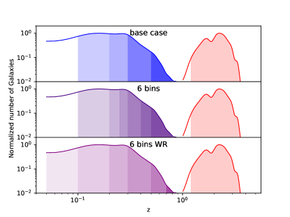
Figure 1: Redshift distributions of the background SMGs (in red) and foreground lenses with the adopted redshift bins indicated by different shades of the same colour. From top to bottom, the ”base case” is shown in blue, the ”6 bins” case in the $0.1<z<0.8$ range in indigo and the ”6 bins WR” case in the wider $0.01<z<0.9$ range in purple, respectively.

2 Methodology

2.1 Data and redshift subsample

The details of the data used for computing the cross-correlation signal are discussed in detail in paper I GON23. Specifically, the background sample is selected from the Herschel Astrophysical Terahertz Large Area Survey (H-ATLAS; Eales et al., 2010) sources in the Galaxy And Mass Assembly (GAMA) fields (G09, G12 and G15) which covers approximately $\sim 147$ deg² of common area and part of the south Galactic pole (SGP), totalling around 60 deg². A photometric redshift selection of $1.2<z<4.0$ was applied to avoid redshift overlap with the lenses. As a result, we obtained a sample of approximately 66,000 sources with an average photometric redshift of 2.20. The redshift distribution of the background sources used in the study is estimated as $p(z|W)$ for galaxies selected by a window function with a redshift range of $1.2<z<4.0$. The distribution takes into account the effect of random errors in photometric redshifts, following the methodology described in González-Nuevo et al. (2017).

The foreground or lens sample used in this work is referred to as the ”z_spec sample” in González-Nuevo et al. (2021), consisting of approximately 150,000 galaxies with redshifts in the range of 0.2 ¡ z_spec ¡ 0.8. These redshift values were obtained from the GAMA II spectroscopic survey. The total common area used in this study was approximately 207 deg². To facilitate our analysis, we divided the foreground sample into different sub-samples based on their redshift. Following the previous results from Bonavera et al. (2021), we adopted the ”base case” which involved dividing the entire redshift range into four bins: $0.1<z<0.2$ (bin 1), $0.2<z<0.3$ (bin 2), $0.3<z<0.5$ (bin 3), and $0.5<z<0.8$ (bin 4).

To investigate the possible dependence on the number of redshift bins but maintaining the same redshfit range, we conducted a joint analysis using six redshift bins, referred to as the ”6 bins” scenario. In this scenario, the entire range was divided into $0.1<z<0.2$ (bin1), $0.2<z<0.25$( bin2a), $0.25<z<0.3$ (bin2b), $0.3<z<0.4$ (bin3a), $0.4<z<0.5$ (bin3b) and $0.5<z<0.8$ (bin4). Finally, we also conducted a joint analysis using six bins of redshift, but with a wider range, denoted as the ”6 bins WR” case. In this case, the range extended from 0.01 to 0.9, with the following bin divisions: $0.01<z<0.1$ (bin 0), $0.1<z<0.2$ (bin 1), $0.2<z<0.3$ (bin 2), $0.3<z<0.5$ (bin 3), $0.5<z<0.7$ (bin 4) and $0.7<z<0.9$ (bin 5).

The redshift distributions of the foreground and background sources are shown in Fig. 1. The bins of redshift adopted in the foreground sample are highlighted with varying shades of the same colour. The three different sets of bins, consisting of four bins, six bins and six bins in a wider range, are displayed from top to bottom in blue, indigo and purple, respectively.

2.2 Measurements

In previous works, the available area is divided in small regular regions, mini-tiles, due to its computational efficiency and accuracy in measuring the angular clustering of galaxies (e.g. González-Nuevo et al., 2017; Bonavera et al., 2019, 2020, 2021; Cueli et al., 2021; González-Nuevo et al., 2021; Bonavera et al., 2022; Cueli et al., 2022). However, it requires an integral constraint (IC) correction to obtain an unbiased estimate of the true function, particularly crucial for constraining cosmological parameters on the largest angular scales. Moreover, using mini-tiles poses a practical challenge as the vertices of each of them must be manually defined, that it is poorly scalable when expanding the study to other wide field surveys observed by Herschel, which might have hundreds of mini-tiles.

To overcome these challenges, we have adopted a statistically rigorous approach that leverages the full field area and combines the number of different foreground-background pairs from each field into a single estimation. This new approach, described in detail in paper I, reduces statistical uncertainty and effectively utilises all available information in the data, as opposed to separately measuring cross-correlation functions for individual fields. The cross-correlation function is then measured using the modified version of the Landy & Szalay (1993) estimator by Herranz (2001),

$$\hat{w}_{\text{fb}}(\theta)=\frac{\rm{D}_{f}\rm{D}_{b}(\theta)-\rm{D}_{f}\rm{R}_{b}(\theta)-\rm{D}_{b}\rm{R}_{f}(\theta)+\rm{R}_{f}\rm{R}_{b}(\theta)}{\rm{R}_{f}\rm{R}_{b}(\theta)},$$ (1)

For every angular separation $\theta$, the $\rm{D}_{f}\rm{D}_{b}$, $\rm{D}_{f}\rm{R}_{b}$, $\rm{D}_{b}\rm{R}_{f}$ and $\rm{R}_{f}\rm{R}_{b}$ represent the normalised foreground-background, foreground-random, background-random and random-random pair counts coming from the whole available area. The background random samples are generated taking into account the surface density variation due to the Herschel scanning strategy.

Furthermore, to estimate the covariance matrix, we employed a Bootstrap method by dividing each field into at least five patches, ensuring a sufficient number of measurements. As explained in Paper I, these patches were created using a k-mean clustering algorithm, ensuring that the spatial dependence structure is retained during resampling. This new methodology has demonstrated enhanced robustness and significantly reduced uncertainties in the obtained measurements. In essence, the overall area was divided into 22 subregions and $N_{b}$=10000 Bootstrap samples were created with an over-sampling factor of 3. Therefore, the covariance matrix is given by

$$\text{Cov}(\theta_{i},\theta_{j})=\frac{1}{N_{b}-1}\sum_{k=1}^{N_{b}}\,\bigg{[}\hat{w}_{k}(\theta_{i})-\bar{\hat{w}}(\theta_{i})\bigg{]}\bigg{[}\hat{w}_{k}(\theta_{j})-\bar{\hat{w}}(\theta_{j})\bigg{]},$$ (2)

where $\hat{w}_{k}$ denotes the measured cross-correlation function from the $k^{\text{th}}$ Bootstrap sample and $\bar{\hat{w}}$ is the corresponding average value over all Bootstrap samples.

In this work, we conduct a tomographic analysis by calculating the cross-correlation functions for each redshift bin defined in the previous section. The cross-correlation measurements, along with the outcomes of each case, are presented in Sect. 3. Specifically, in Fig. 2, we compare the cross-correlation measurements obtained by Bonavera et al. (2021) (light grey circles) with those derived using our new methodology (black circles), thereby confirming the improved results also in the context of tomography.

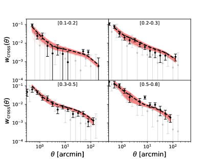
Figure 2: Cross-correlation data (black points) and the results obtained with the tomographic case: the posterior sampling of the cross-correlation function is shown in red and the best fit with the black dashed line. Bin 1 to bin 4 are shown from left to right, top to bottom. For comparison cross-correlation data by Bonavera et al. (2021) are shown in grey.

2.3 Theoretical framework

The low redshift galaxy-mass correlation and the cross-correlation between foreground and background sources are connected through weak lensing. The mass density field traced by the foreground galaxy sample causes weak lensing, and this affects the number counts of the background galaxy sample through magnification bias, as described in detail in paper II. To compute the correlation between the foreground and background sources, we adopt the halo model formalism described in Cooray & Sheth (2002) and the Limber and flat-sky approximations. The correlation can be evaluated using the following equation:

$$\begin{split}w_{\text{fb}}(\theta)=2(\beta-1)\int^{\infty}_{0}\frac{dz}{\chi^{2}(z)}\frac{dN_{f}}{dz}W^{lens}(z)\\ \int_{0}^{\infty}\frac{ldl}{2\pi}P_{\text{g-m}}(l/\chi^{2}(z),z)J_{0}(l\theta)\end{split}$$ (3)

where $W^{\text{lens}}(z)$ is defined as:

$$W^{\text{lens}}(z)=\frac{3}{2}\frac{H_{0}^{2}}{c^{2}}E^{2}(z)\int_{z}^{\infty}dz^{\prime}\frac{\chi(z)\chi(z^{\prime}-z)}{\chi(z^{\prime})}\frac{dN_{b}}{dz^{\prime}}$$ (4)

Here, $E(z)=\sqrt{\Omega_{m}(1+z)^{3}+\Omega_{\Lambda}}$, $dN_{b}/dz$ and $dN_{f}/dz$ are the unit-normalised background and foreground redshift distributions, $\chi(z)$ is the comoving distance to redshift z and $P_{\text{g-m}}$ is the galaxy-matter cross-power spectrum. The logarithmic slope of the background sources number counts is denoted by $\beta$, and the details of our handling of such parameter in the analysis are described in paper II.

Due to the considerable number of integrals that need to be computed for each evaluation of the model, a mean-redshift approximation has been utilised. This approximation involves the evaluation of the outermost integrals in equations 3 not being carried out directly for the entire redshift distribution, but instead through computation at the sample’s mean redshift:

$$w_{\text{fb}}(\theta)\approx 2(\beta-1)\frac{W^{\text{lens}}(\bar{z})}{\chi^{2}(\bar{z})}\int_{0}^{\infty}\frac{ldl}{2\pi}P_{\text{g-m}}(l/\chi(\bar{z}),\bar{z})J_{0}(l\theta).$$ (5)

As detailed in paper II, the cross-power spectrum of galaxies and matter is the power spectrum of the galaxy distribution is expressed as the sum of two terms: the 1-halo term, which describes galaxy-matter correlations within the same halo, and the 2-halo term, which refers to the cross-correlation between different halos.

The cross-correlation function depends on the value of beta and the cosmological parameters of the assumed underlying model, but it also needs information about the way galaxies populate dark matter halos. This is described by the HOD, for which we assume the simple three-parameter model by Zehavi et al. (2005). According to it, when the mass of a halo exceeds a certain threshold, $M_{min}$, a galaxy is located at its centre. Any other galaxies are considered satellites and their distribution is directly proportional to the halo mass profile, as detailed in works such as Zheng et al. (2005). If the mass of a halo exceeds a different threshold, $M_{1}$, it will host satellites, and the number of satellites present is described by a power-law function with a coefficient of $\alpha$.

Consequently, it is possible to represent the probability of a central galaxy being present as a step function:

$$N_{\text{c}}(M)=\cases{0}\quad\text{if}\ M<M_{\text{min}}\\ 1\quad\text{otherwise}{}$$ (6)

The satellite galaxies occupation can be described as:

$$N_{\text{s}}(M)=N_{\text{c}}(M)\cdot\biggl{(}\dfrac{M}{M_{1}}\biggr{)}^{\alpha}$$ (7)

being $M_{\text{min}}$, $M_{1}$ and $\alpha$ the free-parameters of the model.

2.4 Parameter estimation

In order to estimate the parameters, we use the open source software package called emcee, which is licensed under MIT, and utilises a Markov chain Monte Carlo (MCMC) algorithm to estimate the parameters. It is based on the Affine Invariant MCMC Ensemble sampler by Goodman & Weare (2010) and is implemented purely in Python. The MCMC runs in this work are performed with a number of walkers set to three times the number of parameters to be estimated, $N$, and a fixed number of iterations set to 5000. This generates $15,000N$ posterior samples per run, which are then reduced by discarding the initial iterations and introducing a burn-in when flattening the chain. We examined each parameter’s walkers separately to identify the burn-in value. We selected the iterations where all walkers had moved to explore a specific area rather than wandering randomly. The number of iterations we kept depended on the specific case. Finally, we confirmed the chains’ convergence using GETDIST (Lewis, 2019).

In our analysis, we aim to estimate both astrophysical and cosmological parameters. The astrophysical parameters of interest are $M_{min}$, $M_{1}$, and $\alpha$, with different values for each redshift bin. With respect to Bonavera et al. (2021), the parameter $\beta$ is also added to the analysis, since, as studied in paper II, fixing it to the previously used value of 3 could bias the results. On the other hand, the cosmological parameters include $\Omega_{M}$, $\sigma_{8}$, and $h$, which is defined as $H_{0}=100\cdot h\text{km}\text{s}^{-1}\text{Mpc}^{-1}$. We assume a flat universe where $\Omega_{\text{DE}}=1-\Omega_{M}$, and we hold the values of $\Omega_{b}$ and $n_{s}$ fixed at their best-fit values from Planck Collaboration et al. (2021), which are $\Omega_{b}=0.0486$ and $n_{s}=0.9667$, respectively. In the weak lensing approximation, only the cross-correlation function data with angular scales greater than or equal to $0.5$ arcmin are considered, as discussed in detail in Bonavera et al. (2019).

When using the Bayesian method for parameter estimation, it is necessary to define both a prior and a likelihood distribution. For the likelihood distribution, a conventional Gaussian function is employed. In terms of selecting prior distributions for the astrophysical parameters, we use uniform priors. In particular, in the scenarios using the four bins, that is ”base case”, ”w/o G15”, ”bins 14” and ”bins 23”, we adopt the $\log{M_{min}}$ and $\log{M_{1}}$ priors listed in Table 1. In the ”6 bins” case we use the priors specified in Table 2. For the ”6 bins WR” case we choose those in Table 3. For all bins and all cases, $\alpha\sim\mathcal{U}[0.5,1.5]$ and $\beta$ priors are Gaussian with $\beta\sim\mathcal{G}[2.2,0.1]$, following the discussion of paper II.

Table 1: Parameter prior distributions adopted in the scenarios using the four bins, that is ”base case”, ”w/o G15”, ”bins 14” and ”bins 23”.

Parameter	bin 1	bin 2	bin 3	bin 4
$\log M_{\text{min}}$	$\mathcal{U}[10.0,13.0]$	$\mathcal{U}[11.0,13.0]$	$\mathcal{U}[11.5,13.5]$	$\mathcal{U}[12.0,14.5]$
$\log M_{1}$	$\mathcal{U}[11.0,15.5]$	$\mathcal{U}[12.0,15.5]$	$\mathcal{U}[12.5,15.5]$	$\mathcal{U}[13.0,15.5]$

Table 2: Parameter prior distributions adopted in the ”6 bins”.

Parameter	bin 1	bin 2a	bin 2b	bin 3a	bin 3b	bin 4
$\log M_{\text{min}}$	$\mathcal{U}[10.0,13.0]$	$\mathcal{U}[11.0,13.0]$	$\mathcal{U}[11.0,13.0]$	$\mathcal{U}[11.5,13.5]$	$\mathcal{U}[11.5,13.5]$	$\mathcal{U}[12.0,14.5]$
$\log M_{1}$	$\mathcal{U}[11.0,15.5]$	$\mathcal{U}[12.0,15.5]$	$\mathcal{U}[12.0,15.5]$	$\mathcal{U}[12.5,15.5]$	$\mathcal{U}[12.5,15.5]$	$\mathcal{U}[13.0,15.5]$

Table 3: Parameter prior distributions adopted in the ”6 bins WR”.

Parameter	bin 0	bin 1	bin 2	bin 3	bin 4	bin 5
$\log M_{\text{min}}$	$\mathcal{U}[10.0,13.0]$	$\mathcal{U}[10.0,13.0]$	$\mathcal{U}[11.0,13.0]$	$\mathcal{U}[11.5,13.5]$	$\mathcal{U}[12.0,14.5]$	$\mathcal{U}[12.0,14.5]$
$\log M_{1}$	$\mathcal{U}[11.0,15.5]$	$\mathcal{U}[11.0,15.5]$	$\mathcal{U}[12.0,15.5]$	$\mathcal{U}[12.5,15.5]$	$\mathcal{U}[13.0,15.5]$	$\mathcal{U}[13.0,15.5]$

The prior distributions for the cosmological parameters that we aim to estimate are the same as those employed in Bonavera et al. (2020, 2021). More specifically, $\Omega_{M}\sim\mathcal{U}[0.1-0.8]$, $\sigma_{8}\sim\mathcal{U}[0.6-1.2]$, and $h\sim\mathcal{U}[0.5-1.0]$.

3 Results

In this section we describe and discuss the results obtained by jointly analysing different combination of bins of redshift for foreground sample, the lenses. In particular, Sec. 3.1 describes the ”base case”, while Sec. 3.2 study the potential effect in the results due to the anomalous measurements in the G15 field, pointed out in paper I and already analysed in paper II. Finally, in Sec. 3.3 the effect on the constraints of using different number and ranges of bins for the tomographic analysis is discussed. On one hand, we address the possibility of reducing the joint analysis to only a pair of bins (”bins 14” and ”bins 23”), which would diminish the computational time of the parameters estimation. On the other hand, we increase the number of bins to six to explore both the effect of a thinner slicing (”6 bins” case) of the foreground sample in the same redshift range of the ”base case” and the effect of introducing two more bins, one at each end of the four bin case (”6 bins WR” case).

3.1 ”Base case”: four redshift bins

The fist step of our study consists in the comparison between the results obtained with the ”full model” and the mean-redshift approximation, as described in paper II. This approximation reduces the computational time by about a factor of 10 and it is of crucial importance when performing tomographic analyses, given the large number of parameters to be estimated in such a configuration. The same improved data and methodology described in paper I are used in both cases. The comparative plots are shown in appendix A. The HOD parameters prior distributions used for both cases are summarised in Table 1.

Figures 13 and 2 present the posterior sampling of the cross-correlation function (in red), the best fit (dashed black line) and the data (black dots) in the four redshift bins for ”full model” and the mean-redshift approximation, respectively. The panels represent the results for the different bins of redshift, bin 1 to bin 4 from left to right, top to bottom, respectively. The redshift range is indicated in every panel. The data have comparable errorbars in the four bins, except in bin 1 that present larger errorbars at intermediate-large angular scales. Overall, the best fit and sampled area area in good agreement with the data in both cases.

Moreover, Fig. 14 illustrates the marginalised posterior distribution and probability contours for all the estimated parameters. Given the large number of involved parameters, in order to clearly show the results, we divide the corner plot according to the number of bins. In this way we depict the posterior distribution of the HOD parameters of each bin together with the cosmological parameters (that are the same for every bin). With the same aim of making the presentation of the results more intelligible, we decide not to include in the plots the $\beta$ parameter, since its posterior distribution barely deviates from its (Gaussian) prior. As expected, given the small bin ranges used for tomography, the mean-redshift approximation (”base case”) results are in good agreement with the ”full model” case.

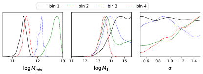
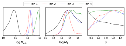
Figure 3: Top: HOD parameters for the tomographic case. Bottom: HOD parameters for the tomographic case excluding the data from the G15 field. The solid black, dashed red, dotted blue and dash-dotted green lines are the bin 1, bin 2, bin 3 and bin 4, respectively. The mass values are expressed in $M_{\odot}/h$ units.

The top panel of Figure 3 displays the marginalised posterior distributions of the HOD parameters for the ”base case”. The solid black, dashed red, dotted blue, and dash-dotted green lines correspond to bin 1, bin 2, bin 3, and bin 4, respectively. A notable trend can be observed, with the value of $\log{M_{min}}$ increasing as a function of redshift from bin 1 to bin 4. The distribution peaks are located at 11.54, 11.56, 12.16, and 12.77, respectively. This behaviour is consistent with previous tomographic analyses (González-Nuevo et al., 2017; Bonavera et al., 2021; Cueli et al., 2022).

Regarding the $\log{M_{1}}$ parameter, the marginalised posteriors appear relatively homogeneous across the four bins, with peaks ranging from 13.44 to 13.85, except for bin 1 which exhibits slightly higher values peaking at 14.67 along with a broader distribution. On the other hand, the $\alpha$ parameter remains poorly constrained in all bins, with only lower limits identified in bin 2 and bin 4, while exhibiting a peak at 0.89 in bin 3.

Comparing our results to those of Bonavera et al. (2021), we generally find narrower distributions and consistent findings. The main discrepancy lies in the $\log{M_{min}}$ distributions for bin 4, where the values obtained in the ”base case” are lower. Additionally, some subtle distinctions can be observed in the opposite trends of the $\alpha$ distributions for bin 2, although it should be noted that $\alpha$ is not constrained in either case.

Figure 4 presents the estimated cosmological parameters for the ”base case” represented by the blue curves. The marginalised distributions exhibit peaks at 0.14 for $\Omega_{M}$ and 0.90 for $\sigma_{8}$. The results from the non-tomographic analysis in paper II and the tomographic analysis by Bonavera et al. (2021) are also displayed in red and green, respectively. The impact of the new methodology, particularly the reduction in measurement uncertainties, is evident for $\Omega_{M}$, as indicated by the significantly narrower posterior distributions compared to the results obtained by Bonavera et al. (2021). However, it is noteworthy that there is a preference for lower values of $\Omega_{M}$, with the posterior distributions deviating considerably from the standard model. This issue will be further explored in the subsequent subsection.

Regarding $\sigma_{8}$, there is good agreement between the tomographic results, with the newer analysis exhibiting a slightly narrower posterior distribution. The higher value observed in the non-tomographic case is consistent with the comparison between the non-tomographic results from González-Nuevo et al. (2021) and the tomographic analysis by Bonavera et al. (2021). Notably, the parameter $h$ remains unconstrained in all three cases.

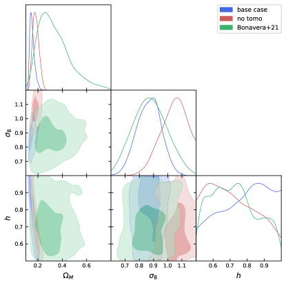
Figure 4: Comparison of the marginalised posterior distribution and probability contours (set to 0.393 and 0.865) for the cosmological parameters obtained in the ”base case” in blue, with single bin form paper II in red and by Bonavera et al. (2021) in green.

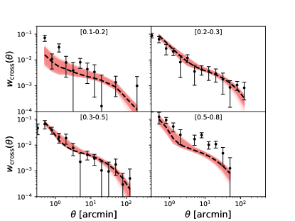
Figure 5: Cross-correlation data (black points) and the results obtained with the tomographic case excluding G15: the posterior sampling of the cross-correlation function is shown in red and the best fit with the black dashed line. Bin 1 to bin 4 are shown from left to right, top to bottom and the redshift ranges are indicated in each panel.

3.2 ”w/o G15”: four redshift bins without the G15 field

The inclusion or exclusion of the G15 field has a significant impact on the measured cross-correlation function at larger angular scales, as previously discussed in paper I. Since the cosmological constraints heavily rely on these angular scales, the effect of the G15 field on the results becomes crucial, as demonstrated in paper II for a broad single redshift bin. In light of this, we explore the potential effects of excluding the G15 field in the tomographic analysis in this study.

The posterior sampling of the cross-correlation function, shown in red in Figure 5, confirms the effect of removing the G15 field on the largest angular scales, resulting in a steeper decrement of the signal. Due to the reduced statistics compared to the case where all four fields are included, the uncertainties of the data are larger. Comparing both sets of measurements, it is evident that the removal of the G15 field leads to a worsening of the best fit and posterior sampling for the bin 1 and, especially, for the highest redshift bin. This can be attributed to the statistical weight of the central bins in the overall best fit due to the relatively better uncertainties in the measurements.

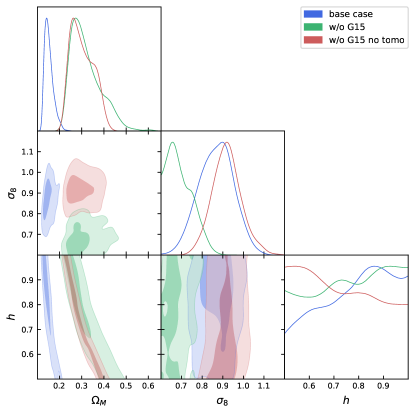
Figure 6: Comparison of the marginalised posterior distribution and probability contours (set to 0.393 and 0.865) of the cosmological parameters obtained in the ”w/o G15” case (in green) and in the corresponding case with single bin from paper II (in red). The ”base case” results are also shown in blue.

Figure 15 displays the posterior distribution of the estimated parameters, organised per bin, similar to Fig. 14. The marginalised posterior distributions of the estimated HOD parameters, presented in the bottom panel of Fig. 3, reveal that, similar to the ”base case,” the $\log{M_{min}}$ parameters exhibit increasing peak values with the bin range. Specifically, the distributions peak at 10.89, 12.16, 12.26, and 12.88 for bin 1 to bin 4, respectively. Comparing with the ”base case” in the upper panel, the main difference lies in the $\log{M_{min}}$ distribution of bin 2, which shifts to higher values when the G15 field is excluded. This shift may be related to the substantial difference in the signal levels observed in bin 2 between these two cases. The parameter $\log{M_{1}}$ displays a similar behaviour to that of the ”base case,” while the $\alpha$ distributions are broad and mostly consistent between the ”base case” and the ”w/o G15” case, except for the opposite trends observed in bin 1 and bin 3.

Figure 6 presents the marginalised posterior distributions and probability contours of the cosmological parameters estimated for the ”w/o G15” case (in green). The marginalised posterior distribution for $\Omega_{M}$ peaks at a higher value of 0.27 compared to the ”base case” (in blue), while it peaks at a lower value of 0.66 for $\sigma_{8}$. The parameter $h$ remains unconstrained. In the same plot, we also compare the results with the corresponding non-tomographic analysis from paper II (in red). The main difference lies in the higher value of $\sigma_{8}$, which peaks at approximately 0.9 in the non-tomographic case, but the qualitative behaviour is the same: the removal of the G15 region produces lower values of $\sigma_{8}$ and larger values of $\Omega_{m}$ both in the non-tomographic and tomographic cases.

In summary, we confirm in this study that the exclusion of the G15 field leads to a decrease in the cross-correlation signal at the largest angular separation distances, as observed in paper I and paper II. While this effect is noticeable in all redshift bins, it is particularly evident across all angular scales in bin 2. Consequently, the main difference with respect to the ”base case” is observed in the $\log{M_{min}}$ distribution for bin 2, which shifts towards significantly higher values. These findings suggest that the anomaly associated with the G15 field may be related to a sample variance problem within the large-scale structure in the line of sight, but particularly within a specific range of redshifts.

3.3 Tomographic analysis with different bins of redshift

In this section, we assess the impact of considering different numbers of redshift bins and exploring different redshift ranges. One interesting aspect to investigate from a computational perspective is the possibility of using only two bins of redshift, which would effectively halve the number of HOD parameters to be estimated compared to the ”base case” (see Sect. 3.3.1). Additionally, we aim to discern the major contributor to cosmological parameter estimation: whether it is more influenced by the extreme redshift bins (”bins 14” case), where the redshift evolution of the measurements plays a prominent role, or the central bins (”bins 23” case), which offer better statistical robustness.

In section 3.3.2, despite not reducing computational time, we further explore the possibilities with a finer slicing of the default redshift range. Specifically, we investigate the potential benefits of jointly analyzing six bins of redshift (”6 bins” case). Lastly, we extend the total redshift range by incorporating two additional bins at the endpoints of the original ”base case” in the foreground sample. Through these analyses, we aim to gain insights into the implications of different redshift binning strategies and explore the trade-offs between computational efficiency and precision in cosmological parameter estimation.

3.3.1 Two-bins analysis

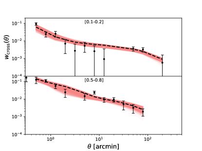
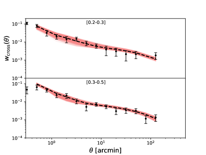
Figure 7: Cross-correlation data (black points), best fit (black dashed line) and the posterior sampling (in red) in the ”bins 14” scenario (left panel) and in the ”bins 23” case (right panel).

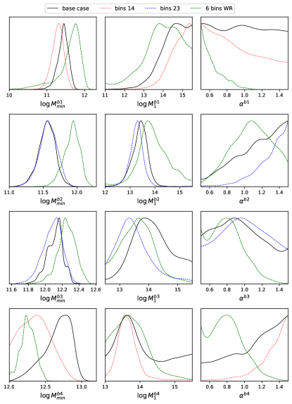
Figure 8: Comparison of the marginalised posterior distributions of the HOD parameters ($\log{M_{min}}$, $\log{M_{1}}$ and $\alpha$ from left to right, respectively) derived in the different analysed cases, for the bin 1, bin 2, bin 3 and bin 4 from top to bottom, respectively. The ”base case” is shown with the black solid line, ”bins 14” with the red dotted line, ”bins 23” with the blue dashed line and the ”6 bins WR” with the green dash-dotted line. The mass values are expressed in $M_{\odot}/h$ units.

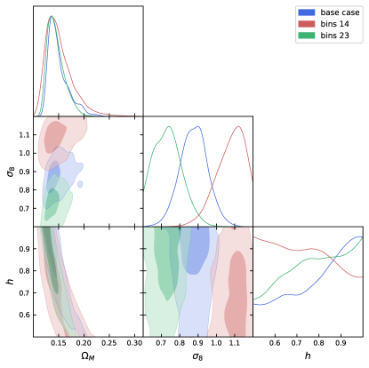
Figure 9: Comparison of the marginalised posterior distribution and probability contours (set to 0.393 and 0.865) of the cosmological parameters obtained in the ”base case” (in blue) and in the two bins cases, ”bins 14” (in red) and ”bins 23” (in green).

The panels in Fig. 7 depict the data (black dots), the posterior sampling of the cross-correlation function (in red) and the best fit (dashed black line) obtained in the joint analysis of bin 1 and bin 4 (”bins 14”, left panel) and in the joint analysis of bin 2 and bin 3 (”bins 23”, right panel). In both cases the upper panel refers to the lowest bin in the pair and the bottom to the highest. The redshift range is indicated in every panel. In most cases the best fit and sampled area are in agreement with the data.

The marginalised and probability distribution are shown in Figs. 16 (for the joint bin 1 and bin 4 case) and 17 (for the joint bin 2 and bin 3 case). As with the previous plots, the results are divided according to the number of jointly analysed bins, two in this case, for a better visualisation.

The HOD marginalised posterior distributions for the two-bins cases are shown in Fig. 8: the red dotted line indicates the results of ”bins 14” and the blue dashed line those of ”bins 23”. These cases are compared with the ”base case” (black solid line) and the common bins in the ”6 bins WR” case. This figure shows the three analysed HOD parameters $\log{M_{min}}$, $\log{M_{1}}$ and $\alpha$ in the columns from left to right, respectively. The four rows represents the four bins, bin 1 to bin 4 from top to bottom.

For the ”bins 14” case, the ${M_{min}}$ parameter in bin 1 is consistent with that of the ”base case,” peaking at 11.32, while in bin 4, it slightly shifts towards lower values, peaking at 12.38. Similarly, the $\log{M_{1}}$ parameter in both bins aligns with the ”base case,” peaking at 15.35 in bin 1 and 13.57 in bin 4. The $\alpha$ parameter remains unconstrained in bin 1 and provides a lower limit in bin 4. In the ”bins 23” case, $\log{M_{min}}$ again agrees with the ”base case,” with peaks at 11.56 in bin 2 and 12.13 in bin 3. The $\log{M_{1}}$ results are also consistent, peaking at 13.31 in bin 2 and slightly lower at 13.32 in bin 3. The parameter $\alpha$ exhibits a lower limit in bin 2 and remains unconstrained in bin 3.

The posterior distributions of cosmological parameters are shown in Fig. 9, with the ”bins 14” case displayed in red and the ”bins 23” case in green. For comparison, the ”base case” is plotted in blue, with uncertainties only slightly improved compared to the other two cases. The marginalised posterior distribution of $\Omega_{M}$ shows good agreement among the three cases, peaking at 0.14. The $\sigma_{8}$ posteriors reveal an intriguing displacement: the distribution for ”bins 23” is shifted to lower values (peaking at 0.74) compared to ”bins 14” (peaking at 1.12), while the ”base case” distribution falls in between (peaking at 0.90). The parameter $h$ remains unconstrained as expected. Tomographic analysis achieves substantial constraining power even with only two redshift bins. However, the discrepancy in $\sigma_{8}$ across the different cases suggests a sample variance issue that can be mitigated by increasing the number of redshift bins. Thus, the sample variance problem identified in paper I, which affected the spatial distribution, also manifests as sample variance in redshift, as hinted by the analysis of the G15 effect in Section 3.2.

3.3.2 Six-bins analysis

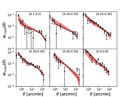
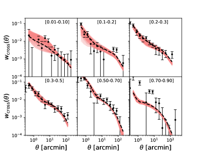
Figure 10: Cross-correlation data (black points), best fit (black dashed line) and sampling posterior (in red) obtained in the ”6 bins” case (left) and the ”6 bins WR” case (right).

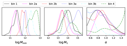
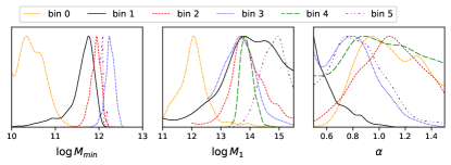
Figure 11: HOD parameters marginalised posterior distributions: $\log{M_{min}}$, $\log{M_{1}}$ and $\alpha$, first, second and third column, respectively. The top panel shows the results for the ”6 bins” case and the bottom panel those for the ”6 bins WR” case. The mass values are expressed in $M_{\odot}/h$ units.

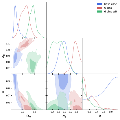
Figure 12: Comparison of the marginalised posterior distribution and probability contours for the cosmological parameters obtained in the ”base case” (in blue) and in the six bins cases, ”6 bins” (in red) and ”6 bins WR” (in green).

Considering the conclusions of the previous section, we investigate the effect of increasing the number of redshift bins in two specific cases: maintaining the same redshift range (”6 bins”) or extending it by adding additional redshift bins (”6 bins WR”). The definition of the redshift bins for both cases was already discussed in Sec. 2.1, and the prior distributions used are summarised in Table 2 and 3, respectively.

The panels in Fig. 10 display the posterior sampling of the cross-correlation function (in red), the best fit (dashed black line), and the data (black dots) for the joint analysis of six bins in the original redshift range (”6 bins” case, left plot) and the wider redshift range from 0.01 to 0.9 (”6 bins WR” case, right plot). Each panel represents the results for a specific redshift bin, and the range of each bin is indicated. In the ”6 bins” case, the data are visibly affected by poorer statistics compared to the ”base case” due to the same total number of sources being spread over more bins. In the ”6 bins WR” case, the central bins show similar behaviour to the ”base case,” while the newly added first and last bins have large error bars due to lower lensing probability (see Lapi et al., 2012) in the first bin and significantly poorer statistics in the last bin. In most cases, the best fit and sampled area align well with the data, except for the last bin in the ”6 bins WR” case, which exhibits poor agreement.

The marginalised and probability distribution of the six-bins analysis are illustrated in Figs. 18 (”6 bins” case) and 19 (”6 bins WR” case). As in the previous cases, the corner plot is divided according to the number of jointly analysed bins, six in this case, for a better visualisation.

Figure 11 displays the marginalised posterior distributions of the HOD parameters for the six-bins cases: the ”6 bins” case in the upper panel and the ”6 bins WR” case in the lower panel. The parameters $\log{M_{min}}$, $\log{M_{1}}$, and $\alpha$ are shown from left to right, and different redshift bins are indicated with various line styles. In the ”6 bins WR” case, the most similar bins to the original ones are represented with the same line style. The additional bins added at the extremes of the original range are depicted with the yellow dash-dotted line (bin 0) and the purple dash-dot-dotted line (bin 5) in the bottom panel.

The ${M_{min}}$ parameter generally increases with redshift, except for bin 2 in the ”6 bins” case, which shows a distribution similar to bin 1, and bin 5 in the ”6 bins WR” case, positioned between bins 3 and 4. This might simply be due to the much larger errobars and less significant signal in such bins, especially bin 5 in the ”6 bins WR” case, which is the one with the worst fit. All the distributions are well constrained showing peaks (from lower to higher bin) at 11.46, 11.37, 11.79, 12.03, 12.39 and 12.77 for the ”6 bins” case and at 10.33, 11.76, 11.95, 12.23, 13.57 and 12.08 for the ”6 bins WR” case. Notably, in the ”6 bins WR” case, the values tend to converge around 12.0 for all redshift bins except bin 0 and bin 4. Fig. 8 compares, for the redshift bins in common, the HOD marginalised posterior distributions of the ”6 bins WR” case (green dash-dotted line) with the other three cases studied in this work. The figure shows again how the $\log{M_{min}}$ values tend to converge toward a value near 12.0.

The marginalised posterior distributions of $\log{M_{1}}$ are very similar in both cases, although the ”6 bins WR” case shows a slight shift towards higher values. The peaks in the ”6 bins” case range from 13.39 to 14.02, with the exception of bin 4, which has slightly higher values (peak at 15.07). In the ”6 bins WR” case, the peaks range from 13.66 to 14.96, except for bin 1, which peaks at a lower value of 12.06. The parameter $\alpha$ does not show a clear trend, as the posterior distributions peak at different values within the available range for both cases.

The marginalised posterior distributions of the cosmological parameters are presented in Fig. 12 in red for the ”6 bins” case and in green for the ”6 bins WR” case. The ”base case” results are plotted in blue for comparison. The marginalised posterior distribution of $\Omega_{M}$ clearly shifts towards higher values, with the ”6 bins” case peaking at 0.23 and the ”6 bins WR” case peaking at 0.29, compared to the ”base case” peak at 0.14. The posterior distributions in both cases are wider than in the ”base case”.

Increasing the number of redshift bins has a similar effect to removing the G15 field, especially when additional bins are added instead of dividing the existing ones. This suggests that the evolution with redshift, i.e. the cosmological model, starts to dominate over the sample variance effect. However, the overall fit is not perfect for each individual bin, resulting in poorer fits for the most biased samples. Extending the redshift range seems to work better than simply increasing the number of redshift bins, as it improves statistics per bin and produces tighter constraints compared to the ”w/o G15” case.

The $\sigma_{8}$ posterior distribution for the ”6 bins WR” case is compatible with the ”base case” results but shows a wider distribution towards lower values, with a peak (mean) value at 0.84 (0.80). In contrast, the ”6 bins” case exhibits a clear peak at 1.08. This difference can be attributed to the splitting of the two central bins, which reduces their statistics compared to bin 1 and bin 4, resulting in a lower weight in the parameter estimation and producing estimates similar to the ”bins 14” case.

Finally, the parameter $h$ remains unconstrained, but for the first time in this work, the posterior distributions show tight upper limits of 0.78 and 0.73 at 95%C.I., in the ”6 bins” and ”6 bins WR” respectively in both cases. These results align with the findings in paper II, where a joint analysis of the cross-correlation function and galaxy clustering measurements was performed. Although these results should be interpreted with caution, they indicate that with improved data and better-constrained parameters, there is hope for obtaining constraints on $h$.

4 Conclusions

This study is the third in a series that examines various aspects associated with the study of the submillimeter galaxy magnification bias, with a specific focus on the tomographic scenario. It is akin to the work carried out by Bonavera et al. (2021), but using the updated data from Paper I. The objective is to refine the methodology employed in constraining the free parameters of the HOD model, that is $M_{min}$, $M_{1}$, and $\alpha$, and the cosmological parameters $\Omega_{M}$, $\sigma_{8}$, and $h$ of a flat $\Lambda$CDM model on a tomographic scenario.

Due to the large number of parameters that must be jointly analysed in tomography, a significant amount of computational time is required to accomplish this kind of task. Therefore, one of the aims of this work is to explore ways to optimise CPU time and strategies for analysing different redshift bins without compromising the precision of the measurements. Various data-sets have been explored to this end, which involve the combination of different redshift bins and the inclusion/exclusion of the G15 field suspected to have an anomalous behaviour. Each data-set consists in the measurement of the cross-correlation function between background H-ATLAS submillimeter galaxies and foreground GAMA galaxies within a tomographic setup.

As in Bonavera et al. (2021) and Cueli et al. (2022) we divide the entire redshift range into four bins: bin 1 ($0.1<z<0.2$), bin 2 ($0.2<z<0.3$), bin 3 ($0.3<z<0.5$), and bin 4 ($0.5<z<0.8$). In the ”base case” and ”w/o G15” scenarios, we examine all four bins together, including SGP and all the GAMA fields and excluding the G15 field, respectively.

We first compare the ”base case” which makes use of the mean-redshift approximation with the ”full model” case. This approximation reduces the computational time by about a factor of 10 and it is of crucial importance when performing tomographic analyses, given the large number of parameters to be estimated in such a configuration. The comparative plots confirm that given the thinness of the redshift bins used for tomography, the ”base case” results are in good agreement with the ”full model” case.

The marginalised posterior distributions exhibit a systematic increase in $\log{M_{min}}$ from bin 1 to bin 4 as redshift increases, while the distributions of $\log{M_{1}}$ show relatively consistent values across the four bins. In addition to the HOD parameters, we compare the inferred cosmological parameters with the results obtained from the non-tomographic runs in paper II and the tomographic analysis conducted by Bonavera et al. (2021). The impact of our new methodology, particularly the reduction in measurement uncertainties, becomes evident when examining $\Omega_{M}$, as indicated by the considerably narrower posterior distributions compared to the findings of Bonavera et al. (2021). However, it is worth noting that our results exhibit a preference for lower values of $\Omega_{M}$, with the posterior distributions deviating noticeably from the predictions of the standard model.

In relation to the ”w/o G15” scenario, our study confirms the findings of paper I and paper II, which demonstrate that excluding the G15 field results in a reduction of the cross-correlation signal at larger angular separations. While this effect is observed across all redshift bins, it is particularly pronounced in bin 2, affecting all angular scales. As a result, the most significant deviation from the ”base case” is observed in the $\log{M_{min}}$ distribution for bin 2, which shifts towards notably higher values. These observations suggest that the peculiar behavior associated with the G15 field might be attributed to sample variance within the large-scale structure along the line of sight, particularly within a specific range of redshifts.

For the sake of computational efficiency, we narrow our focus to the joint analysis of two bin pairs: ”bins 14” (the first and fourth bin) and ”bins 23” (the second and third bin). Remarkably, the HOD parameters obtained from these analyses are consistent with those of the ”base case”. The marginalised posterior distribution of $\Omega_{M}$ exhibits strong agreement across all three cases, peaking at 0.14. However, the $\sigma_{8}$ posteriors reveal an intriguing disparity: the distribution for ”bins 23” is shifted towards lower values (peaking at 0.74), whereas ”bins 14” yields higher values (peaking at 1.12), and the ”base case” falls in between (peaking at 0.90). This discrepancy suggests the presence of sample variance in redshift, which can be mitigated by increasing the number of redshift bins. Thus, the sample variance issue identified in paper I, which affected the spatial distribution, also manifests as sample variance in the redshift domain, as implied by the analysis of the G15 effect.

We investigate the impact of increasing the number of redshift bins in two cases: ”6 bins” (maintaining the same redshift range) and ”6 bins WR” (extending the range with additional bins). In the ”6 bins” case, the data are affected by poorer statistics due to the same number of sources being spread over more bins. In the ”6 bins WR” case, central bins resemble the ”base case,” while newly added first and last bins have larger error bars and significantly poorer statistics.

The marginalised posterior distributions of $\log{M_{1}}$ and $\alpha$ are very similar in both cases. The $\log{M_{min}}$ distributions are well-constrained, with peaks increasing with redshift as expected. In the ”6 bins WR” case, the values show a convergence around the value 12.0 for most bins. The $\Omega_{M}$ distribution shifts towards higher values, peaking at 0.23 in the ”6 bins” case and 0.29 in the ”6 bins WR” case, compared to the ”base case” peak at 0.14. Increasing the number of redshift bins has a similar effect as removing the G15 field, suggesting the dominance of the cosmological model over sample variance. However, individual bin fits are not perfect, resulting in poorer fits for the most biased samples. Extending the redshift range improves statistics and produces tighter constraints compared to the ”w/o G15” case.

The $\sigma_{8}$ posterior distribution for the ”6 bins WR” case is compatible with the ”base case” results but shows a wider distribution towards lower values, with a peak (mean) value of 0.84 (0.80). In contrast, the ”6 bins” case exhibits a clear peak at 1.08. This difference is due to reduced statistics in the two central bins compared to bin 1 and bin 4, producing estimates more similar to the ”bins 14” case. The parameter $h$ remains unconstrained, but the posterior distributions show tight upper limits in both cases, consistent with previous findings in paper II.

As a concluding remark, this study contributes to refining the methodology for tomographic analyses and highlighted the importance of considering sample variance and redshift binning in obtaining precise measurements of HOD and cosmological parameters. The spatial sample variance, and probably also the redshift one, can be minimised by increasing the number of independent fields, such as incorporating additional Herschel wide area surveys, such us the Herschel Multi-tiered Extragalactic Survey (HerMES; Oliver et al., 2012) or the Great Observatories Origins Deep Survey-Herschel (GOODS-H; Elbaz et al., 2011). However, our results also indicate that enhancing both the number of redshift bins and the redshift range yields more accurate and robust outcomes, mitigating the potential impact of both types of sample variance. To implement this second approach effectively, it is important to adopt updated foreground catalogues with improved statistics for our purposes, such as the Dark Energy Survey (DES; The Dark Energy Survey Collaboration, 2005) or the future Euclid mission (Euclid Collaboration et al., 2022).

Appendix A Comparison ”full model” and ”base case”

This appendix presents the results obtained in the ”base case” and the original model, ”full model” which is used in previous works (e.g. González-Nuevo et al., 2017; Bonavera et al., 2020, 2021, 2022; Cueli et al., 2021, 2022). The jointly analysed bins of redshift and the priors are the same in both runs. Figure 13 shows the cross-correlation data (black points), the best fit (black dashed line) and the sampled area (in red) obtained with the MCMC. The agreement with the data is good as well as with the findings in Fig. 2.

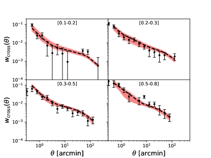
Figure 13: Cross-correlation data (black points) and the results obtained with the full model with no approximations: the black dashed line shows the best fit and the red lines are the sampling posteriors.

Moreover, we show in red the marginalised posterior distributions and probability contours (set to 0.393 and 0.865) in Fig. 14. Even if the analysis is jointly performed among the four bins, due to the large amount of parameters to be shown in the figure, we split such results into four panels. Each panel shows the HOD estimated parameters for one bin together with the cosmological parameters, that are the same for the four panels. In particular, bin 1 to bin 4 are shown from left to right, top to bottom respectively. In this figure we also show in blue the results of the ”base case” where we adopt the mean-redshift approximation, detailed described in paper II which consists in computing the outer integrals in equation 3 at the mean redshift of the sample (see equation 5). In the tomographic analysis performed in this work we can safely adopt such approximation, given the small range of redshift in each in bin.

The results of this two cases are in very good agreement and the subsequent analyses in this work can be safely performed with it. It provides great advantages from the computational point of view, especially in the tomographic analysis which involves a large number of parameters.

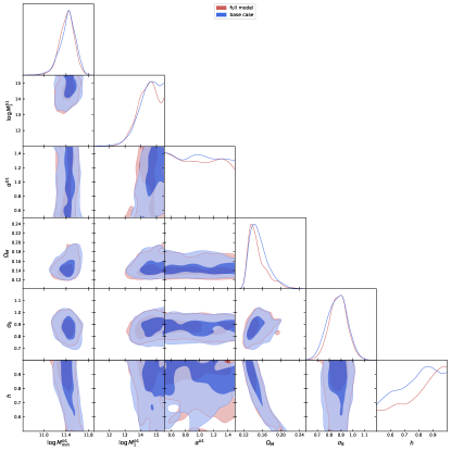
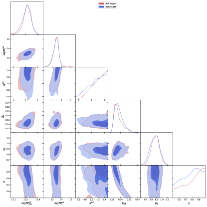
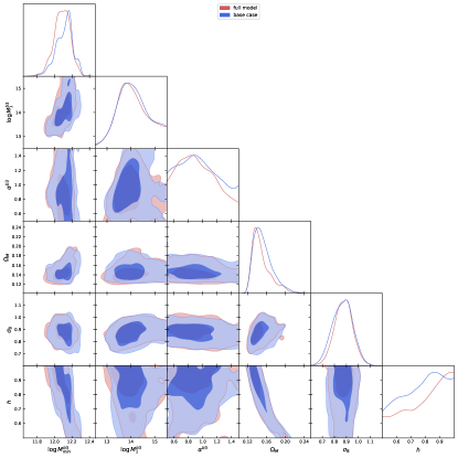
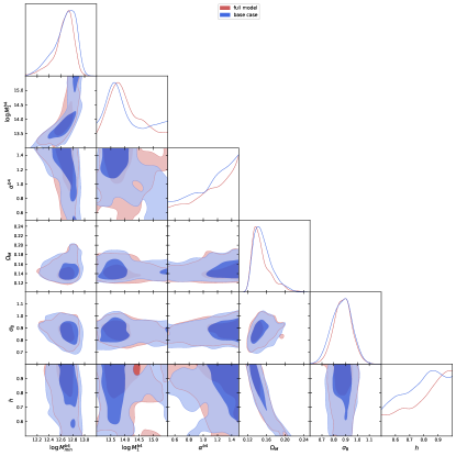
Figure 14: Comparison of the marginalised posterior distribution and probability contours (set to 0.393 and 0.865) for the HOD and cosmological parameters obtained in the ”base case” (in blue) and in the ”full model” case (in red).

Appendix B Posterior distributions of the individual cases

This section presents the marginalised posterior distributions and probability contours (set to 0.393 and 0.865) of all the cases addressed in this work and compared to the ”base case” presented in section A. In particular, Fig. 15 show the case corresponding to Sect. 3.2 in which the joint analysis is performed on the four bins bin 1, bin 2, bin 3 and bin 4 without taking into account the G15 field.

The two bins case described in Sect. 3.3.1, where only two bins are jointly analysed are shown in Figs. 16 and 17. In particular, Fig. 16 corresponds to the ”bins 14” case, where just bin 1 and bin 4 are jointly analysed and Fig. 17 shows the results obtained in the ”bins 23” case, that is considering only bin 2 and bin 3.

The six bins cases in Sect. 3.3.2 are depicted in Figs. 18 and 19. Fig. 18 describes the findings of the ”6 bins” case, which are attained using bin 1, bin 2a and bin 2b (by splitting bin 2), bin 3a and bin 3b (by splitting bin 3) and bin 4. Fig. 19 shows the ”6 bins WR” case, obtained adding two extra bins to the ”base case”: bin 0 (to the lower end of the original case, $0.01>z>0.1$), bin 1, bin 2, bin 3, bin 4 (but only up to z=0.7 to increase the statistics of bin 5) and bin 5 ($0.7>z>0.9$).

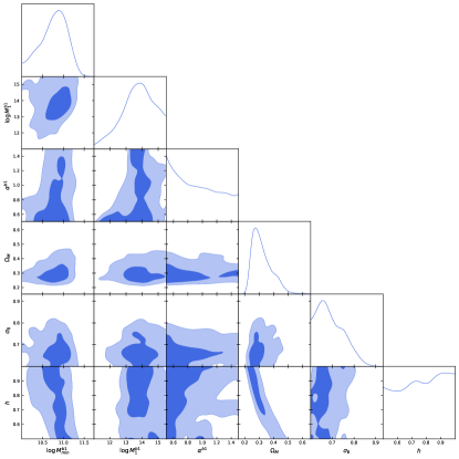
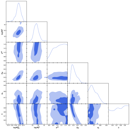
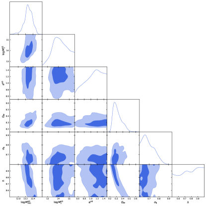
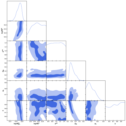
Figure 15: Marginalised posterior distribution and probability contours (set to 0.393 and 0.865) for the HOD and cosmological parameters obtained in the ”w/o G15” case.

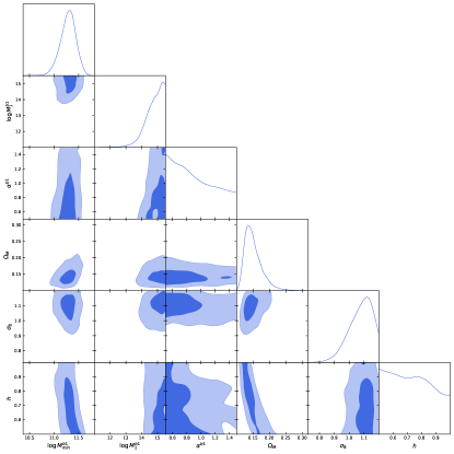
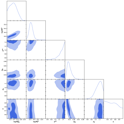
Figure 16: Marginalised posterior distribution and probability contours (set to 0.393 and 0.865) for the HOD and cosmological parameters obtained in the ”bins 14” case.

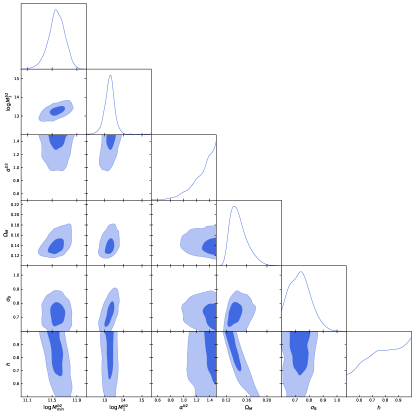
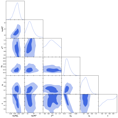
Figure 17: Marginalised posterior distribution and probability contours (set to 0.393 and 0.865) for the HOD and cosmological parameters obtained in the ”bins 23” case.

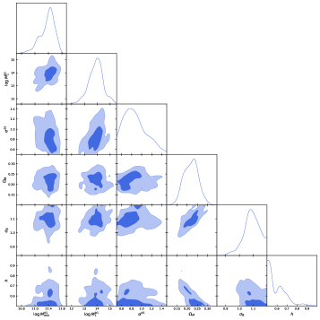
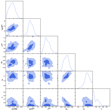
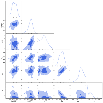
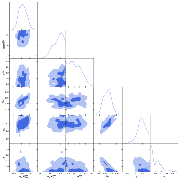
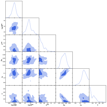
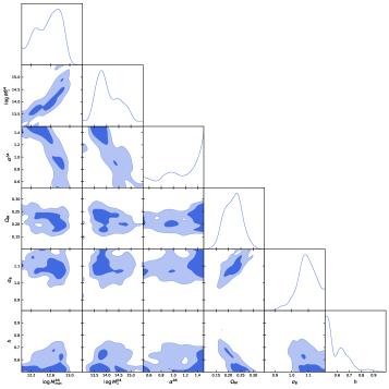
Figure 18: Marginalised posterior distribution and probability contours (set to 0.393 and 0.865) for the HOD and cosmological parameters obtained in the ” 6 bins” (i.e. $0.1<z<0.8$) case.

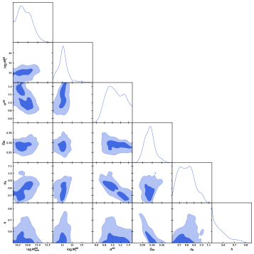
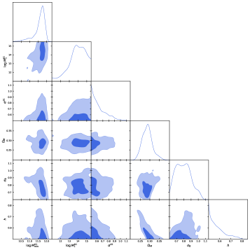
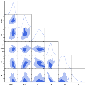
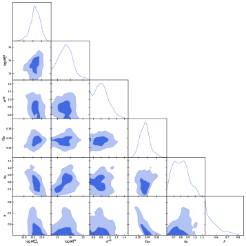
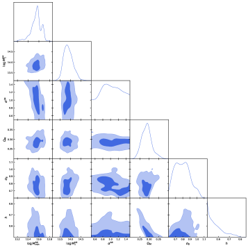
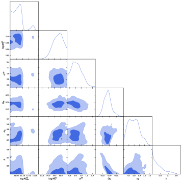
Figure 19: Marginalised posterior distribution and probability contours (set to 0.393 and 0.865) for the HOD and cosmological parameters obtained in the ” 6 bins WR” (i.e. $0.01<z<0.9$) case.

References

- Bacon et al. (2000) Bacon, D. J., Refregier, A. R., & Ellis, R. S. 2000, Monthly Notices of the Royal Astronomical Society, 318, 625
- Bakx et al. (2020) Bakx, T. J. L. C., Eales, S., & Amvrosiadis, A. 2020, MNRAS, 493, 4276
- Bianchini et al. (2015) Bianchini, F., Bielewicz, P., Lapi, A., et al. 2015, ApJ, 802, 64
- Bianchini et al. (2016) Bianchini, F., Lapi, A., Calabrese, M., et al. 2016, ApJ, 825, 24
- Blain (1996) Blain, A. W. 1996, MNRAS, 283, 1340
- Bonavera et al. (2022) Bonavera, L., Cueli, M. M., & Gonzalez-Nuevo, J. 2022, Proceedings of the MG16 Meeting on General Relativity, R. Ruffini & G. Vereshchagin eds., World Scientific., arXiv:2112.02959
- Bonavera et al. (2021) Bonavera, L., Cueli, M. M., González-Nuevo, J., et al. 2021, A&A, 656, A99
- Bonavera et al. (2020) Bonavera, L., González-Nuevo, J., Cueli, M. M., et al. 2020, A&A, 639, A128
- Bonavera et al. (2019) Bonavera, L., González-Nuevo, J., Suárez Gómez, S. L., et al. 2019, J. Cosmology Astropart. Phys., 2019, 021
- Bussmann et al. (2012) Bussmann, R. S., Gurwell, M. A., Fu, H., et al. 2012, ApJ, 756, 134
- Bussmann et al. (2013) Bussmann, R. S., Pérez-Fournon, I., Amber, S., et al. 2013, ApJ, 779, 25
- Calanog et al. (2014) Calanog, J. A., Fu, H., Cooray, A., et al. 2014, ApJ, 797, 138
- Cooray & Sheth (2002) Cooray, A. & Sheth, R. 2002, Phys. Rep, 372, 1
- Cueli et al. (2022) Cueli, M. M., Bonavera, L., González-Nuevo, J., et al. 2022, A&A, 662, A44
- Cueli et al. (2021) Cueli, M. M., Bonavera, L., González-Nuevo, J., & Lapi, A. 2021, A&A, 645, A126
- Eales et al. (2010) Eales, S., Dunne, L., Clements, D., et al. 2010, PASP, 122, 499
- Elbaz et al. (2011) Elbaz, D., Dickinson, M., Hwang, H. S., et al. 2011, A&A, 533, A119
- Euclid Collaboration et al. (2022) Euclid Collaboration, Scaramella, R., Amiaux, J., et al. 2022, A&A, 662, A112
- Fu et al. (2012) Fu, H., Jullo, E., Cooray, A., et al. 2012, ApJ, 753, 134
- González-Nuevo et al. (2021) González-Nuevo, J., Cueli, M. M., Bonavera, L., et al. 2021, A&A, 646, A152
- González-Nuevo et al. (2017) González-Nuevo, J., Lapi, A., Bonavera, L., et al. 2017, J. Cosmology Astropart. Phys., 2017, 024
- González-Nuevo et al. (2012) González-Nuevo, J., Lapi, A., Fleuren, S., et al. 2012, ApJ, 749, 65
- Goodman & Weare (2010) Goodman, J. & Weare, J. 2010, Communications in Applied Mathematics and Computational Science, 5, 65
- Herranz (2001) Herranz, D. 2001, in Cosmological Physics with Gravitational Lensing, ed. J. Tran Thanh Van, Y. Mellier, & M. Moniez, 197
- Hildebrandt et al. (2013) Hildebrandt, H., van Waerbeke, L., Scott, D., et al. 2013, MNRAS, 429, 3230
- Hunter (2007) Hunter, J. D. 2007, Computing In Science & Engineering, 9, 90
- Jones et al. (2001) Jones, E., Oliphant, T., Peterson, P., et al. 2001, SciPy: Open source scientific tools for Python
- Landy & Szalay (1993) Landy, S. D. & Szalay, A. S. 1993, ApJ, 412, 64
- Lapi et al. (2012) Lapi, A., Negrello, M., González-Nuevo, J., et al. 2012, The Astrophysical Journal, 755, 46
- Lewis (2019) Lewis, A. 2019 [arXiv:1910.13970]
- Ménard et al. (2010) Ménard, B., Scranton, R., Fukugita, M., & Richards, G. 2010, MNRAS, 405, 1025
- Nayyeri et al. (2016) Nayyeri, H., Keele, M., Cooray, A., et al. 2016, ApJ, 823, 17
- Negrello et al. (2017) Negrello, M., Amber, S., Amvrosiadis, A., et al. 2017, MNRAS, 465, 3558
- Negrello et al. (2010) Negrello, M., Hopwood, R., De Zotti, G., et al. 2010, Science, 330, 800
- Negrello et al. (2007) Negrello, M., Perrotta, F., González-Nuevo, J., et al. 2007, MNRAS, 377, 1557
- Oliver et al. (2012) Oliver, S. J., Bock, J., Altieri, B., et al. 2012, MNRAS, 424, 1614
- Pérez & Granger (2007) Pérez, F. & Granger, B. E. 2007, Computing in Science and Engineering, 9, 21
- Planck Collaboration et al. (2021) Planck Collaboration, Aghanim, N., Akrami, Y., et al. 2021, A&A, 652, C4
- Rhodes et al. (2001) Rhodes, J., Refregier, A., & Groth, E. J. 2001, The Astrophysical Journal, 552, L85
- Schneider et al. (1992) Schneider, P., Ehlers, J., & Falco, E. E. 1992, Gravitational Lenses
- Scranton et al. (2005) Scranton, R., Ménard, B., Richards, G. T., et al. 2005, ApJ, 633, 589
- The Dark Energy Survey Collaboration (2005) The Dark Energy Survey Collaboration. 2005, arXiv e-prints, astro
- Van Waerbeke et al. (2000) Van Waerbeke, L., Mellier, Y., Erben, T., et al. 2000, A&A, 358, 30
- Wardlow et al. (2013) Wardlow, J. L., Cooray, A., De Bernardis, F., et al. 2013, ApJ, 762, 59
- Wittman et al. (2000) Wittman, D. M., Tyson, J. A., Kirkman, D., Dell’Antonio, I., & Bernstein, G. 2000, Nature, 405, 143
- Zheng et al. (2005) Zheng, Z., Berlind, A. A., Weinberg, D. H., et al. 2005, ApJ, 633, 791