Mitigating the Performance Impact of Network Failures in Public Clouds

Abstract. Some faults in data center networks require hours to days to repair because they may need reboots, re-imaging, or manual work by technicians. To reduce traffic impact, cloud providers mitigate the effect of faults, for example, by steering traffic to alternate paths. The state-of-art in automatic network mitigations uses simple safety checks and proxy metrics to determine mitigations. SWARM, the approach described in this paper, can pick orders of magnitude better mitigations by estimating end-to-end connection-level performance (CLP) metrics. At its core is a scalable CLP estimator that quickly ranks mitigations with high fidelity and, on failures observed at a large cloud provider, outperforms the state-of-the-art by over 700$\times$ in some cases.

1. Introduction

Data center networks often incur a variety of (concurrent) failures ranging from failed or lossy links to localized, persistent congestion. It takes time to repair these failures (GCP, [n. d.]); e.g., operators require days to replace optical links and hours to fix hardware-induced packet corruptions (Wu et al., 2012; Bogle et al., 2019; Gao et al., 2020; Zhuo et al., 2017).

Cloud providers install mitigations to reduce the impact of failures while they work on repairs. With the economic importance of cloud services and the increasing likelihood of failures at scale, it is crucial to find and implement effective mitigations quickly. In this paper, we focus on network-level mitigations such as disabling links or switches, re-routing traffic, etc. These are effective because of the path and resource diversity in data center networks.

Nowadays, cloud providers are turning to automation to find effective mitigation for each failure. For instance, ProviderX utilizes automation for nearly $80\%$ of its incidents. An auto-mitigation system allows an operator to pre-define a limited set of potential mitigations for each type of failure. The system then chooses the “best” mitigation for each individual incident. Thus, at its core, an auto-mitigation system ranks mitigations based on one or more criteria. To be effective, it must do so quickly; data at ProviderX shows mitigation must be in place within $5$ minutes (see also (Gao et al., 2020)) of operators localizing the failure.

ProviderX uses local criteria to assess mitigations. For example, disabling a link is acceptable if it leaves sufficient functional uplinks at the corresponding switch. The start of the art either uses non-local criteria, such as the residual path diversity from the ToRs to the spine of the data center (Zhuo et al., 2017), or global but non-end-to-end measures like packet loss and network utilization (Wu et al., 2012). But these methods can negatively impact customers by suggesting inadequate mitigations (§2).

In this paper, we explore a mitigation ranking criterion which prior work does not consider — the global impact of the mitigation on the end-to-end connection-level performance (CLP) across all connections in the data center. Our CLP measures include flow throughput and flow completion time (FCT). We quantify the global impact using distributional measures of these quantities (averages and percentiles). Failures can adversely impact these measures, for instance, by lowering the 1st percentile (1p) throughput due to a reduction in capacity: an ideal mitigation is the one that minimizes the drop in 1p throughput relative to the original network.

From the cloud operator’s perspective, this criterion completely captures the network performance all customers experience and is preferable to local or non-end-to-end criteria, which may not always directly relate to customer-visible network performance. But at the scale of today’s data centers, it is unclear if it is possible to quickly rank mitigations by global end-to-end CLP measures.

We introduce SWARM, a service for operators and auto-mitigation systems that quickly ranks mitigations while scaling to large clusters. SWARM leverages the insight that ranking mitigations only requires an estimate of CLP distributions with enough fidelity to produce effective orderings. SWARM uses a CLP estimator that approximates the distribution of CLP metrics: it models traffic, routing, and transport behavior in sufficient detail to ensure ranking fidelity and at the same time produces results in just a matter of minutes.

To estimate CLP, SWARM must estimate per-flow performance not just for the current network state (topology and routing), but for potential (unknown) future network states (e.g., additional failures or repairs) which may manifest while a mitigation is in place. Flow performance can depend on other concurrent flows, and flow arrivals and departures. Taking all these into account, while producing an estimate quickly, is the central challenge SWARM faces.

SWARM overcomes these challenges as follows (§3):

• SWARM takes as input distributions of flow arrivals, sizes, and communication probabilities. It uses these to sample a set of flow-level traffic demands to ensure statistical significance. For each such demand, it generates routing samples to capture uncertainty in flows’ paths. SWARM combines the CLP estimates from each combination of routing and traffic samples to create a composite distribution which succinctly captures traffic and routing variability. It then uses this distribution to rank mitigations.

• SWARM estimates CLP separately for long and short flows. Estimating CLP for short flows is easier, since they experience less time varying network behavior. SWARM takes care in modeling long flows along two dimensions: whether their throughput is limited by loss or contention, how this limitation changes over time as flows arrive and depart and network bottlenecks shift during the course of the flow’s lifetime.

• To compute quick estimates, it uses a suite of aggressive scaling methods which include pipelining, parallelism, topology downscaling, and careful data structure design.

It is beneficial to rank CLP estimates: SWARM can explicitly account for failure characteristics (e.g., packet drop rate); it can reason about a broader range of mitigations (taking no action, bringing back a previously disabled link, or adjusting WCMP (Zhou et al., 2014) weights); it can also model failures that prior work (Wu et al., 2012; Zhuo et al., 2017) cannot (e.g., packet drops below the ToR).

SWARM’s design is guided by our experience working with operators of a large production cloud, ProviderX. We discuss the nuances and requirements derived from operator experience and describe how SWARM improves the state of practice. In summary, we make the following contributions:

• We propose CLP-aware failure mitigation, which finds the mitigation with the least impact on network performance. This is a significant departure from state-of-the-art.

• We identify sufficient approximations that allow us to build a robust and scalable CLP estimator that helps rank mitigations effectively and supports a wider range of failures and mitigations compared to prior work.

• We empirically show SWARM is fast at scale and useful: For common failure scenarios (Scenarios 1 and 2 in §4), it picks either the best mitigation or one that is at most $9$% worse. It also outperforms the state-of-the-art by up to 793x. In more complicated failure cases which many prior work (Zhuo et al., 2017; Wu et al., 2012) do not support (Scenario 3 in §4), SWARM picks an action that is at most $29\%$ worse than the best mitigation.

Ethics. This work does not raise any ethical issues.

2. CLP-aware Mitigation

In this section, we use simplified versions of real-world incidents at ProviderX (Figure 1) to explain the limitations of state-of-art auto-mitigation techniques and to illustrate the benefit of global CLP-based impact assessments.

The failure scenario. In the Clos topology of Figure 1, frame check sequence (FCS) errors (Zhuo et al., 2017) appear on a link (FCS). Operators mitigate this failure, but before they can physically replace the link, a fiber cut on another (Link Cut) causes congestion and packet loss.

We simulate (in Mininet (Lantz et al., 2010), details in §4) a sequence of flow arrivals and successively apply each mitigation (or a combination of them) for FCS and Link Cut. For this example, our goal is to maximize the 1st percentile (1p) throughput. We show examples where ProviderX’s troubleshooting guide, CorrOpt (Zhuo et al., 2017), and NetPilot (Wu et al., 2012) lead to substantial and unnecessary performance degradation.

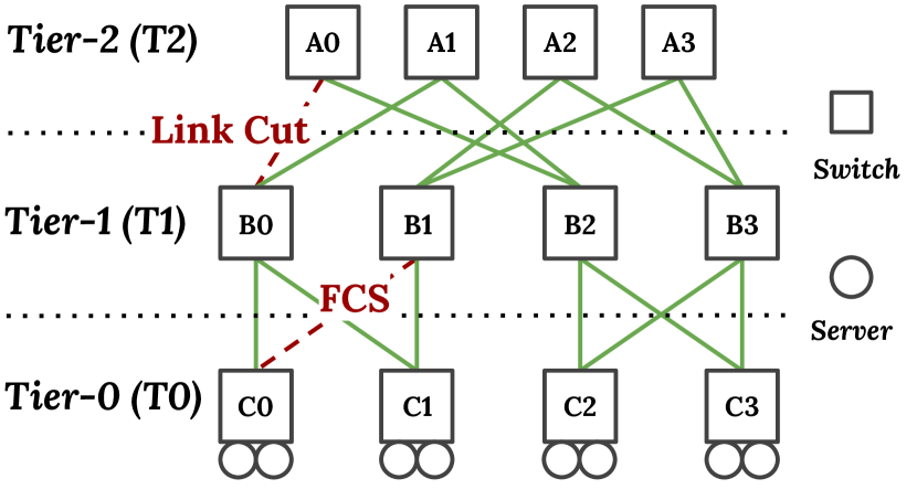
Figure 1. An example of two consecutive failures. First, the link between C0 and B1 experiences frame check sequence (FCS) errors. After mitigating, but before fixing this failure, a fiber cut between A0 and B0 causes congestion-induced packet drops.

Troubleshooting guides. ProviderX’s automation and troubleshooting guides disable any failed link (with drop rate $\geq O(10^{-6})$) if at least half of the switch uplinks are healthy. This mitigation for FCS achieves a 1p throughput of 3.6 Mbps. This decision might be optimal when the drop rates are high (e.g., High FCS with a drop rate of $O(10^{-2})$) but it is conservative, static, and ignores the failure pattern, link location, and traffic demand. For example, at a loss rate of $O(10^{-5})$, leaving the lossy link in place and taking no action has a higher 1p throughput (14.2 Mbps), while disabling the link causes congestion which impacts tail performance. For Link Cut, ProviderX’s guidelines do not do anything in the face of congestion, which results in a 1p throughput of 2.7 Mbps — the 1p throughput is higher if we adjust WCMP (Zhou et al., 2014) weights to reduce traffic on congested links (3.2 Mbps).

CorrOpt (Zhuo et al., 2017). CorrOpt disables the link in FCS if there is sufficient path diversity to the spine/core. This is sub-optimal for the same reason discussed above: depending on the failure properties (e.g., drop rate and location), taking no action may lead to a higher 1p throughput. CorrOpt focuses on FCS errors and does not consider congestion induced by capacity drops, like Link Cut.

NetPilot (Wu et al., 2012). For High FCS, NetPilot always disables the link — not doing so would increase the loss rate (one of the health metrics in NetPilot). This is not always the best option: In a Low FCS scenario (with $O(10^{-5})$ drop rate), we can reduce the 1p throughput from 15 Mbps to 3.6 Mbps if we disable the link. After the Link Cut, NetPilot proceeds to disable the congested link or switch (to avoid additional packet drops), which exacerbates the problem — the 1p throughput reduces to 3.17 Mbps. A better strategy is to undo a previous mitigation and re-enable the Low FCS link when Link Cut occurs: the 1p throughput of this is 14.2 Mbps.

Takeaways. While this is a simplified example, operators can negatively impact customers in practice and cause extended outages if they fail to find an effective mitigation (Azu, [n. d.]). Rules with static thresholds in troubleshooting guides cannot capture correct mitigations because CLP impact depends on traffic demands. Local path diversity measures (as in CorrOpt) cannot capture customer impact since they do not account for the failure characteristics. Non end-to-end metrics like packet loss or utilization (as in NetPilot) often suggest disabling links, which discounts better mitigations. By using CLP, SWARM can rank mitigations by global impact on end-to-end measures.

3. SWARM Design

In this section, we describe how SWARM ranks mitigations in terms of their impact on CLP measures, throughput and FCT. §3.4 discusses failures and mitigations SWARM supports.

3.1. Challenges and Insights

Challenges. Network operators seek to improve CLP objectives which they often specify in terms of distributional statistics (average, percentiles) across the entire data center (e.g., 99th percentile or 99p FCT). To achieve this, SWARM must estimate these distributions quickly and with sufficient accuracy to ensure effective mitigation ranking. This is hard:

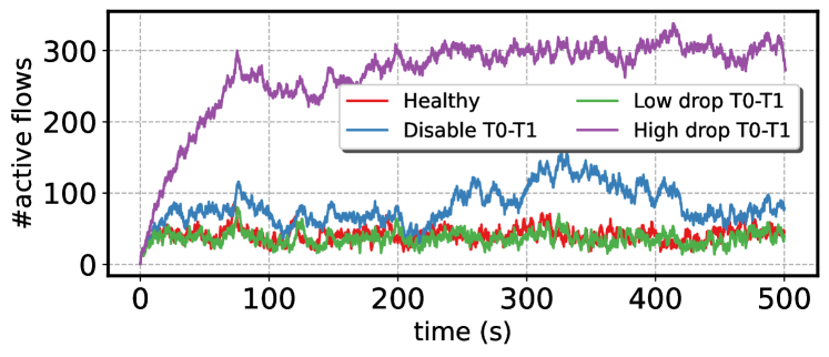
Figure 2. When mitigations keep faulty links up or reduce capacity, flow durations increase, resulting in more active flows.

Traffic characterization. SWARM needs a characterization of traffic demands to estimate CLP distributions for a given failure and mitigation. Instantaneous flow or ToR-level traffic matrices (TMs) can provide such a characterization. Unfortunately, fine-grained flow-level TMs are impractical at data center scales, and ProviderX does not capture them. They are also highly variable under failure; for instance, packet drops often extend the FCT, which can increase the concurrently active flows by $3$-$4\times$ (Figure 2). ToR-to-ToR TMs, as used by NetPilot (Wu et al., 2012), are too ambiguous since they aggregate flows with different behaviors under failure (e.g., a long flow is impacted more by capacity drops).

Routing. Routing determines contention at each link, which impacts throughput and FCTs. How the network routes flows can depend on ECMP hash functions, as well as the existing failures in the network. For example, ECMP hash functions can change when links fail or switches reboot (Sarykalin et al., 2008). SWARM must account for these factors.

Transport behavior. SWARM needs to model transport behavior since CLP measures depend on factors such as congestion controls (e.g., New-Reno vs. Cubic), their parameters (e.g., initial window size), and their reaction to failures (e.g., packet drops). But it is hard to choose the right abstraction level and maintain scalability. Accurate simulations over-index on specific protocols and take too long (Henderson et al., 2008). Faster approximate simulators do not account for lossy links (Zhao et al., 2022; Zhang et al., 2021) or require a prohibitive amount of compute (Zhao et al., 2022; Zhang et al., 2021). Existing formal models are limiting (see §6); e.g., fluid models (Kelly, 2003) capture steady-state for long flows, but datacenter flows are often short and do not reach steady state (Montazeri et al., 2018).

Temporal and spatial flow dependencies. CLP measures depend on the time-varying number of flows competing for bandwidth at a link. They also depend on where (and for how long) these flows are bottlenecked. For instance, a flow bottlenecked elsewhere does not need its full fair share at another link. These bottlenecks might shift frequently due to the arrival and departure of flows. SWARM must efficiently account for these dependencies.

Approach. At the core of SWARM (Figure 3) is a CLPEstimator that estimates the distribution of flows’ throughput and completion times (FCT) for a given network, failure pattern, and mitigation set.

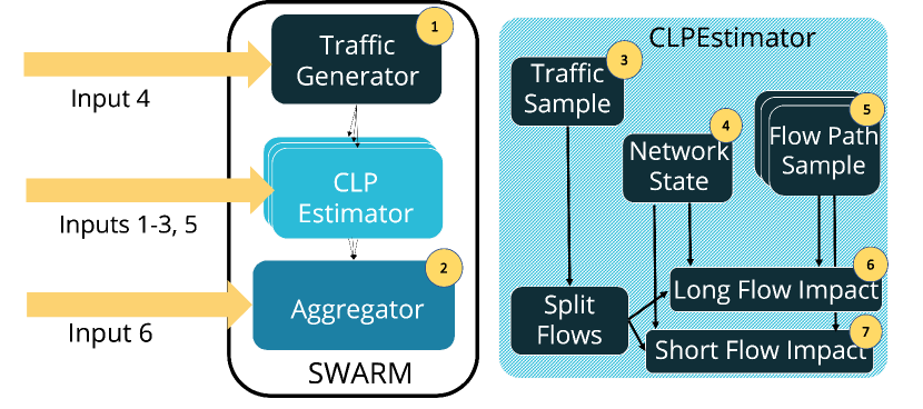
Figure 3. SWARM Design.

SWARM avoids the limitations of fine-grained flow-level TMs and uses an approximate TM distribution (§3.2). It generates multiple ( ) TM samples ( in Figure 3) from three inputs that operators such as ProviderX already collect: the flow arrival rates, their size distributions (Montazeri et al., 2018), and the probability of server-to-server communication (Arzani et al., 2020).

To robustly estimate CLP distributions without exact flow routing information, SWARM samples multiple potential paths ( ) for the given network state (e.g., with or without a failure or mitigation, ) for each flow to ensure a desired statistical confidence (§3.3).

Perhaps the trickiest challenge is to model the impact of losses and dependencies between concurrent flows on throughput and FCT. To this end, SWARM uses two techniques.

First, SWARM addresses changes in bandwidth over time and flow dependencies through a fast and scalable epoch-based flow rate estimator. Specifically, it divides time into multiple epochs, recomputes CLPs in each epoch, and stitches the results to find an overall estimate. Within every epoch, it estimates throughput and FCT for short ( ) and long flows ( ) separately since network failures impact these in different ways: larger flows stay in the network longer and are influenced by the variations in the network state but short flows only experience a snapshot of the network and have more predictable FCTs.

Second, SWARM uses an approximate model of TCP-friendly transport protocols that share a common objective: they grab the flow’s fair share of the bottleneck bandwidth in the absence of failures. To achieve this in the presence of failures and packet drops, SWARM needs to check whether long flows are capacity or loss-limited. For capacity-limited flows, it needs to compute their fair share of bandwidth. For loss-limited flows, it needs to capture the bandwidth their control loop converges to under loss. To achieve this, SWARM extends existing max-min fair algorithms (Jose et al., 2019) .

SWARM aggregates distributions ( ) from each traffic and routing sample, and operators use these to rank mitigations: they can set priorities based on one or more distributional metrics (e.g., prioritize average throughput over FCT).

3.2. SWARM: Inputs and Outputs

Failure	Mitigation	Works that consider these failures/actions
Packet drop above the ToR	Take down the switch or link	NetPilot, CorrOpt, Operators
	Bringing back less faulty links to add capacity	$\times$
	Changing WCMP weights	$\times$
	Do not apply any mitigation	$\times$
Packet drop at ToR	Disable the ToR	Operators
	Move traffic e.g., by changing VM placement	$\times$
	Do not apply any mitigation	$\times$
Congestion above the TOR	Disable the link	NetPilot, Operators
	Disable the device	NetPilot, Operators
	Bring back less faulty links to add capacity	$\times$
	Change WCMP weights	$\times$
	Do not apply any mitigation	$\times$

Table 1. The list of failures and mitigating actions we consider in our design of SWARM.

Inputs. Operators or auto-mitigation tools can invoke SWARM with the following inputs:

1. The topology of the data center.

2. A list of ongoing mitigations (if any).

3. Failure pattern (e.g.,estimated loss rate) and location.

4. Data center traffic details (e.g., TMs distributions).

5. Candidate mitigations to evaluate.

6. A comparator that ranks mitigations by CLP estimates.

Inputs 1-2-3. Operators (e.g., ProviderX) use monitoring systems (Case et al., 1989; Lonvick, 2001) and automated watchdogs (Gao et al., 2020) to detect incidents and use different techniques (such as those in (Wu et al., 2012; Zhang et al., 2018; Arzani et al., 2016)) to localize the failure. They then create incident reports (Gao et al., 2020) that contain details of the incident. Operators or their automation systems use these to install mitigations that are active until the operator finds the root cause and repairs the failure. ProviderX’s automitigation system uses these incident reports, and so does SWARM. The failure characterization (e.g., packet drop rate) is sometimes imperfect in these reports and operators may not be able to accurately localize the failure. SWARM can tolerate errors in packet drop rate (§4), and operators can incorporate the probability of different locations (§5) and iteratively refine mitigations to deal with imperfect localization.

Input 4. SWARM requires simple characterizations of datacenter traffic: the flow arrival distribution, the server-to-server communication probability, and the flow size distributions. From these, it extracts a set of flow-level demand matrices (§3.3). These probabilistic characterizations of the inputs allows SWARM to be robust to traffic variability and ensure a desired level of statistical confidence in its estimation.

Input 5. SWARM takes a list of mitigations as an input to evaluate. Similar to existing troubleshooting guides at cloud providers, operators provide to SWARM a mapping from failure types to a list of mitigations or a combination of mitigations (see §2, e.g., disabling a link and undoing a prior mitigation). Some mitigations might require additional inputs (candidate VM placements or WCMP weights); we assume operators use existing techniques (Supittayapornpong et al., 2022; Grandl et al., 2014) to find values for these inputs. Table 1 shows a sample of failures and associated mitigations.

Input 6. Operators can customize the comparator. Our current implementation supports two types of comparators, and we can easily extend it to support others (see §4). The priority comparator considers throughput-based, and FCT-based metrics (e.g., the $1$-percentile throughput or the $99$-percentile FCT) in a pre-specified priority order. The linear comparator is a linear combination of two or more of these metrics, where the operator specifies the weights.

Outputs. SWARM outputs the mitigation (or mitigation combination) with minimal impact as ranked by the comparator.

3.3. SWARM: Internals

The CLPEstimator (Figure 3). This takes as input a demand matrix ($\mathcal{T}$) and a mitigation ($\mathcal{M}$) and estimates: (a) the distribution of average throughput across all the long flows, and (b) the distribution of FCT accross all the short flows in $\mathcal{T}$. SWARM can compute average throughput from FCT and vice versa using $FCT=\frac{flow\ size}{throughput}$ if needed. SWARM calls the CLPEstimator for each candidate mitigation and ranks them based on the estimates. This section presents the key ideas underlying CLPEstimator (see also Algorithm 2).

How SWARM uses CLPEstimator. SWARM samples $K$ different demand matrices ( in Figure 3) and invokes the CLPEstimator for each of them to evaluate a given mitigation. It selects the different demand matrices, $K$, to achieve a desired level of confidence (see below). CLPEstimator then internally generates $N$ different routing samples ( ), where each sample describes paths flows in the demand matrix take. It chooses $N$ to ensure a desired level of confidence (see below). For each demand and routing sample, SWARM obtains a distribution of throughput and FCT for long and short flows.

From all of these, depending on the comparator, SWARM estimates the distribution of the percentiles of throughput and FCT across these traffic and routing samples (Figure 4). Formally, it computes the distribution of the ordered statistics of the throughput and FCT through empirical observations. For example, if the comparator is based on 99p FCT, SWARM would extract the 99p from FCT distributions of each of the $N\times K$ samples. These values form a composite distribution of the 99p FCTs. The variance of this distribution captures the statistical significance of our estimates in the presence of various sources of uncertainty: the uncertainty in the input distributions (e.g., variance) translates to a corresponding uncertainty in our estimates. We can reduce the uncertainty and improve the confidence in our estimates by increasing the number of samples (Cormode et al., 2012).

SWARM uses the composite distribution ( ) to compare and rank mitigations. This approach allows it to explicitly handle uncertainty and provide robust mitigation rankings.

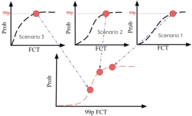
Figure 4. The composite distribution of 99p FCT obtained from many randomly generated traffic and routing samples.

Network state representation. SWARM models the state of the network ( ) using a graph $G=(\mathcal{V},\mathcal{E})$ where each edge $e$ has a capacity and a drop rate (0% = healthy and 100% = completely down), each node $v$ has an associated drop rate and a routing table, and each server $s$ has a mapping to a switch. At the beginning of each invocation (line 2 in Algorithm 2), SWARM updates this state to reflect mitigation $\mathcal{M}$. It uses a careful choice of data structures to ensure that this step is efficient (§3.4).

Modeling traffic variability. The demand matrix $\mathcal{T}$ consists of the arrival times, sizes of flows, and their corresponding source and destinations. To create $\mathcal{T}$, SWARM uses input 4 ( ): for each flow, it samples the flow arrival distribution, randomly determines a source-destination pair from the server-to-server communication probabilities, and flow size from the size distribution. SWARM invokes CLPEstimator with $K$ demand matrix samples. To determine $K$, given a confidence level $\alpha$ it uses the DKW inequality, which provides confidence bounds for the difference between an empirically sampled distribution and the underlying distribution from which the samples are drawn (Dvoretzky et al., 1956).

Modeling routing uncertainty. CLPEstimator handles routing uncertainty by generating $N$ different flow path samples ( ), each representing a different routing of the flows (§3.1). It first uses the DKW inequality (Dvoretzky et al., 1956) to determine the $N$ to achieve a confidence level of $\alpha$. Then, it samples from the distribution of possible paths between source-destination pairs. For this, it computes the probability of a specific path for a given source-destination pair based on routing tables and associated WCMP weights at each node (Figure 5).

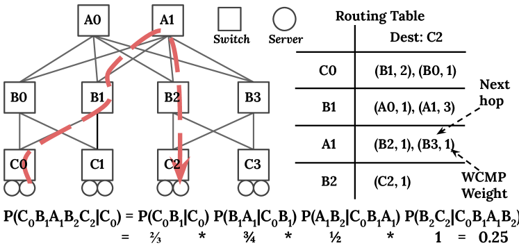
Figure 5. The probability of a flow between two servers taking a particular path.

Modeling the throughput of long flows. As described above, SWARM models long ( ) and short ( ) flows separately. Long flows typically reach their steady state and their throughput depends upon network variations and packet drops, as described below.

Varying network conditions. SWARM approximates network variations and the arrival and departure of flows that compete on a link by dividing time into discrete epochs (Algorithm 1). It assumes stable conditions within the epoch (no flow arrival/departure) but allows for variations across them. At the beginning of each epoch, SWARM adds the newly arrived flows (Line 1) to the set of active flows. Then, it computes their bandwidth share (Line 1). At the end of each epoch, SWARM updates the number of transmitted bytes for each flow, removes the completed flows, and records their overall throughput estimates (Line 1-Line 1).

Input: $G$. current network state.

Input: $\mathcal{T}$ = {<src, dst, size, start time>}.

Input: $\mathcal{P}$. (sample) Set of paths for all flows.

Input: $\mathcal{I}\subset\mathcal{T}$. measurement interval.

Input: $\zeta$. epoch size.

Output: $\beta_{l}$. distribution of throughput of long flows

1 $\mathcal{K}\leftarrow\{\}$

2 $time\leftarrow 0$

3 $\beta_{l}\leftarrow[]$

4 while $\exists\;f\in\mathcal{T}:\;f.start\geq time\;or\;\mathcal{K}\neq\varnothing$ do

5       $time\leftarrow time+\zeta$

6       $\mathcal{K}.add(\{f\in\mathcal{T}:\;time-\zeta\leq f.start<time\})$

7       $\theta_{f}\leftarrow compute\_throughput(G,\mathcal{K},\mathcal{P})$

8       for flow f in $\mathcal{K}$ do

9             $f.sent\leftarrow min(f.sent+\zeta\theta_{f}$, f.size)

10             if $f.sent=f.size$ then

11                   $\mathcal{K}.remove(f)$

12                   if $f\in\mathcal{I}$ then

13                        $\beta_{l}.append(\frac{f.size}{f.dur})$

14                   end if

15                  

16             end if

17            

18       end for

19      

20 end while

return $\beta_{l}$

Algorithm 1 Impact on Long Flows.

Computing bandwidth share. SWARM finds the rate of each flow within an epoch in two steps (Line 1 in Algorithm 1):

1. It computes the loss-limited throughput of each flow, as described below.

2. It executes a demand-aware extension of the water-filling approach in (Jose et al., 2019) (this algorithm provably converges in $O(|E|)$ where $E$ is the number of edges) where it uses these estimates as an upper bound on the flow throughput. We have developed this extension (see  §A.2).

Modeling loss-limited throughputs. While it is possible to find the throughput under packet drop rate analytically, these models are tied to specific congestion control protocols and can not easily extend to other variants (e.g., (Alizadeh et al., 2010)). SWARM overcomes this limitation by using an empirically-driven distribution of the loss-limited throughputs. To find this distribution, SWARM measures the average throughput of a long flow under different network conditions (e.g., drop rate, latency) through experiments in a small testbed. In each experiment, it makes sure link capacities are high enough that they never become bottlenecks, so the drop rate is the only limiting factor. For each network condition, SWARM repeats the experiment multiple times (Dvoretzky et al., 1956) to create a robust distribution. It uses this distribution in step (1) above to sample the drop-limited throughputs. See §B for details.

Modeling the FCT of short flows. Prior work (Mellia and Zhang, 2002) develops an analytical model for the average FCT across flows. We are unaware of any models that estimate the distribution. For SWARM, a simple empirical model for estimating the FCT distribution of short flows suffices — their FCTs are more predictable since they do not stay in the network long enough to be affected by network variations.

SWARM finds the distribution of short flow FCT ( ) by estimating: (a) its RTT; and (b) the number of RTTs to deliver its demand. A short flow’s FCT is equal to the average duration of RTTs times the number of required RTTs. We derive the distribution of each metric separately and use probability theory to combine them and compute the FCT distribution.

We use experiments in a small testbed, with packet drop rates and RTT variations that match those of the data center, to compute (offline) the distribution of the number of RTTs needed to deliver a flow’s demand (for different flow sizes). We store these results in a table that maps the network state and flow properties (e.g., flow size, slow start threshold, initial congestion window) to this distribution.

Next, we estimate the RTT: the sum of the propagation delay (a constant determined by the flow’s path) and the queueing delay along the flow’s path. To estimate queueing delay, we gather data resulting from sending small flows on links with different utilization and active flow counts ( §B).

SWARM combines these distributions to derive the distribution of the FCT for short flows as the sum of the propagation delay and queueing delay multiplied by the number of RTTs.

3.4. Expressivity, Scaling and Robustness

SWARM supports more failures and mitigations than prior work, can be applied iteratively for robustness and incorporates many scaling techniques for speed.

Expressivity. SWARM supports any failure and mitigation if we can present it as changes in the state of the network or the traffic. It does not need the root cause of a failure or details of a mitigation action, but only needs to model the failure’s or mitigation’s observable impact (e.g., packet drop, port down). As a result of this flexibility, SWARM supports a wide variety of failures and mitigations (Table 1). ProviderX commonly observes these failures. Existing production and state-of-the-art systems  (Wu et al., 2012; Zhuo et al., 2017) do not support many of these failures and mitigations.

Robustness. SWARM’s network-level mitigations mask network failures. This masking is not perfect, and a cloud service might react to a mitigation (or, more generally, a failure), thereby changing the traffic demand (e.g., using retries). Precisely for this reason, SWARM does not model a fixed traffic demand, but draws enough traffic demand samples from historical statistics of flow arrivals, sizes, and communication probabilities to ensure statistical significance (§3.3). When operators don’t have such statistics (e.g., after a previously unseen failure, or a data center expansion), SWARM uses a distribution that captures maximum uncertainty (Robinson, 2008).

Although SWARM carefully models uncertainty its CLP estimates may not match CLP estimates operators observe after installing a mitigation. This can happen, for instance, if a relatively rare failure manifests itself that the sampling process did not capture. In these cases, the auto-mitigation system that uses SWARM must update its inputs and invoke it again to revise its decision — mitigation does not have to be a single shot process and can be revised over time especially since failure diagnosis might take hours to days (Gao et al., 2020; Wu et al., 2012).

Scaling. Naïve implementations of SWARM may have unacceptably long run times, even on small topologies. We scale SWARM as follows:

An ultra-fast max-min fair computation algorithm. We use an approximate computation of network-wide max-min fair share rates (max, [n. d.]), which provides significant speedup over the state-of-art methods (Jose et al., 2019) without affecting quality.

Efficient network state and traffic update. The demand matrix is independent of network state and SWARM computes the demand samples offline. But SWARM must re-compute routing samples when it invokes CLPEstimator and has to update the network state to reflect each mitigation before doing so. To make this fast SWARM separates how it represents the topology (as a graph, §3.3) from how it represents demand: it sorts the latter into a list of tuples (source and destination server, flow size, and flow start time). With this design, we can, for example, disable a device (switch or link) by changing drop rate in $G$ to 100%; or if a mitigation modifies the demand (e.g., a VM Migration), we can update the demand matrix.

Parallelism and pipelining. SWARM invokes CLPEstimator for different demand and routing samples in parallel. It also parallelizes and pipelines routing sample generation with epoch execution.

Reducing the number of epochs. After these steps, the bottleneck is the number of epochs in Algorithm 1. We shorten this in two ways. We first initialize the algorithm on warmed-up networks which we draw from historical data. This eliminates the effect of cold-start. Second, we leverage the observation that epochs that are far apart from each other in time present an independent snapshot of the network with a non-overlapping set of flows. So, we can compute their CLPs independently and in parallel. Then, we can stitch the results to form a distribution across all the flows.

Traffic Down Scaling. Following POP (Narayanan et al., 2021), SWARM down-scales the demand matrix, with minimal impact on throughput and splits a network with link capacity $c$ into $k$ sub-networks with link capacity $\frac{c}{k}$ and divides traffic randomly across these sub-networks. This works with any flow arrival distribution; we use Poisson distributions (Kassing et al., 2017; Ghobadi et al., 2016; Mellette et al., 2020; Teh et al., 2020) where the results are the same if we assign flows randomly vs if we down-scale the arrival rate.

4. Evaluation

SWARM outperforms the state of the art, is accurate, and scales well. We first summarize our main findings:

1. In the scenario that most frequently occurs in production, it reduces the performance penalty on 99p FCT by 793$\times$ compared to the next-best system while maintaining comparable average throughput. In other scenarios, it either matches or significantly outperforms other systems.

2. It always chooses a mitigation whose CLP impact is within 9% of the optimal for the most common failure scenarios and at most 29% worse than the optimal on more complicated failures. SWARM considers twice the number of mitigations than the next-best system, choosing to take no action in more than 35% of runs.

3. SWARM finds the best mitigation for a network with over $16$K servers in $\leq 5$ minutes.

4.1. Methodology

Implementation. We have implemented a prototype of SWARM in Python. Our implementation consists of 1500 lines of code.

Metric. We evaluate each approach by computing the Performance Penalty (%): the relative difference between the CLP metrics that result from the best possible mitigation and the one each technique suggests — the best mitigation thus results in a performance penalty of zero. This metric captures the unnecessary performance degradation caused by a technique choosing sub-optimal mitigation. Often, the difference between the best mitigation and the “runner up” is insignificant, which results in a small penalty. In contrast, the difference between the best mitigation and the one the baselines choose can be as high as 200%.

Experimentation setup. We evaluate SWARM both through experiments using Mininet (Lantz et al., 2010) and a physical testbed. Our experimental setup is as follows (see §C for further details):

Traffic characterization. Our distributions for the number of active flows per server per minute use ProviderX production logs; flow size distributions are from DCTCP (Alizadeh et al., 2010).

Simulation Setup. Like (Ros-Giralt et al., 2021), we use Mininet for most of our evaluation, as this gives us control over the topology, but we extend it to improve the analysis and fidelity of our results. We add to Mininet monitoring that captures throughput and latency and we also enable support for various queueing disciplines. We report results on over 50 experiments which represent 4000 experiment-hours and use the Clos (Greenberg et al., 2009; Singh et al., 2015) topology in Figure 1 for our baseline comparisons.

We seek to emulate a topology with a flow arrival rate of $1500$ flows per second per server which results in $12,000$ flows per second arriving in the network, and $40$ Gbps links where each link has $50\mu$s propagation delay. However, running Mininet on a VM with 64 cores and 256GB cannot emulate this traffic demand. We thus downscale, by 120$\times$, traffic demand and link capacities (see§3.4). We run each emulation for $250$ seconds each on $30$ different traces derived from our traffic characterization. We warm-start the emulation to avoid capturing effects from an empty network.

Testbed Setup. Our testbed employs a Clos topology of six TORs, four T1s, and two T2 switches, all connected by 10Gbps links. All switches are Arista 7050QX-32. Each of our six racks contain five to six servers. We introduce random packet loss in the testbed by using a user-defined ACL to match bits on the IP ID field in packet headers and directly modify the Broadcom firmware to drop packets the ACL matches. Because of this, packet loss rates in the testbed are powers of two, based on the number of bits the ACL matches on. We evaluate the impact of the failure and each mitigating action on the testbed with a traffic load of 3000 flows per second over 15 traces derived from our traffic characterization.

SWARM Parameters. We use 32 different random traffic matrices, each 200 seconds long, to estimate the impact of each mitigation. We generate 1000 independent routing samples per traffic, and we compute the CLP metrics over all the flows that start within [50, 150) seconds. Each epoch is 200ms. We also consider any flow with a size $\leq 150KB$ short.

Baselines. We compare SWARM to:

NetPilot (Wu et al., 2012).:

Given a failure, NetPilot iterates through each possible mitigation, computes the maximum link utilization, and picks the mitigation that minimizes utilization. Because NetPilot does not model link utilization on faulty links, it always disables corrupted links. We report these results as NetPilot-Orig. We also extend NetPilot to only mitigate only if the resulting maximum link utilization is below a threshold. We report these results as NetPilot-80 for an 80% and NetPilot-99 for a 99% link utilization threshold.

CorrOpt (Zhuo et al., 2017).:

CorrOpt only considers link corruption failures. CorrOpt disables a link that corrupts packets if the number of paths to the spine that remain once it disables the link is above a threshold. We consider three thresholds, CorrOpt-25 uses a threshold of 25% of paths remaining, CorrOpt-50 uses 50%, and CorrOpt-75 uses 75%.

Operator playbooks.:

If an FCS error occurs above the TOR where there is path redundancy, the ProviderX playbook (also used by their automitigation system) would disable the affected link when the number of uplinks at the switch that remain is above a threshold. We consider three thresholds: Operator-25 uses a 25% threshold, Operator-50 uses 50%, and Operator-75 uses 75%. (2) If there is packet loss of more than $10^{-3}$ at the TOR or below, the playbook would drain the affected nodes (an expensive operation that risks VM reboots or interrupts). Otherwise, it would take no action.

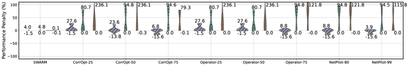
() PriorityFCT

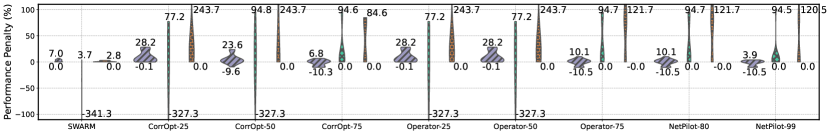
(a) PriorityAvgT

Figure 6. Scenario 1: Comparing the performance penalty by SWARM to baselines. SWARM achieves 793x lower performance penalty on 99p FCS in the worst case compared to the next best baseline (CorrOpt-75) on PriorityFCT. SWARM is the only technique that achieves near-optimal performance across all three metrics (less than 7% penalty) and performs equally well across both comparators. Note, some baselines have a performance penalty as high as $200\%$ on some metrics.

Some baselines result in a partitioned network under certain failure scenarios (in-part due to the smaller scale in our evaluations due to Mininet). For a fair comparison, unless noted otherwise, for baseline comparisons, we only report results when all baselines result in a connected network.

Comparators. Most experiments use two priority comparators (§3.2) (§D.3 shows SWARM achieves low penalty across two other comparators including a linear one as well):

PriorityFCT:

minimizes the 99p FCT. It uses two tiebreakers, 1p throughput followed by average throughput.

PriorityAvgT:

maximizes the average throughput first, using two tiebreakers, 99p FCT, followed by 1p throughput.

Two mitigations are tied on a particular metric if they are within 10% of each other on that metric.

4.2. Baseline Comparisons

We evaluate SWARM over three different failure scenarios which are common in production incidents on ProviderX.

Scenario 1: Link-level packet corruption with network redundancy. In this scenario, $2$ links consecutively experience FCS errors. Links fail with high O($10^{-2}$) or low O($10^{-5}$) packet drop rates. We evaluate all combinations of two-link failures on the topology of Figure 1. This is the most common failure pattern at ProviderX where any drop rate above $O(10^{-6})$ is an incident. Here, the following mitigations are viable: doing nothing, disabling the link, undoing past mitigations and bringing back links that have been already taken down, changing WCMP weights, or any subset of these. All baselines support this scenario (but some fail to support other scenarios) because the link failure is above the TOR and there is path redundancy.

Figure 6 compares the performance penalty of SWARM to the baselines for both comparators. We do not compare to NetPilot-orig in this scenario since the network was partitioned in 16 out of 32 failure pairs and the results on the remaining failure pairs were not statistically significant. We use violin plots to show the distribution of performance penalty across all failure patterns for each candidate approach and each metric. A tall violin plot indicates that performance penalties span a wide range, while a short and wide plot indicates penalties are clustered within a small set of values. Even though baselines do not explicitly use comparators, the best mitigation depends on the choice of the comparator (as the comparator informs the notion of “best”), this causes the performance penalty to change for the baseline under different comparators.

SWARM outperforms all baselines with a performance penalty consistently close to zero. In Figure 6() which uses the Priority-FCT to prioritize 99p FCT, SWARM has a maximum FCT performance penalty of 0.1%, compared with the 79.3% penalty of the closest baseline CorrOpt-75. In Figure 6(a), which uses Priority-AvgT to prioritize average throughput, SWARM’s maximum penalty on average throughput is similar to several of the baselines, such as NetPilot-99 and CorrOpt-75. But SWARM reduces the performance penalty across all three CLP metrics (for both comparators) while the baselines suffer from high performance penalties across at least one. SWARM outperforms the baselines because it can analyze a large space of mitigations and choose one that reduces performance impact on all CLP metrics. Occasionally, it consistently improves a CLP metric (e.g., the 1p throughput for PriorityAvgT) across most failure patterns (negative performance penalty).

Figure 7 depicts the diversity of SWARM’s mitigation choices. It shows the fraction of times SWARM chose each mitigation across all failure patterns under each comparator. SWARM chooses to take no action in more than 35% of the failure patterns. In two cases under PriorityFCT, it not only takes no action on the second failure, but also reinstates the faulty link it previously disabled from the first failure (action NoA/BB/E). Despite two links dropping packets, because of the locations of the failures, their intensity, and the traffic demands, SWARM finds it better to preserve those links rather than eliminate their capacity and cause congestion. Under PriorityAvgT, SWARM chooses multiple mitigations (e.g., disabling both links and adjusting WCMP weights).

We next evaluate SWARM on two other scenarios we derive from production to highlight its properties and to illustrate shortcomings in existing approaches.

Scenario 2: Congestion on a link. Operators shut down a number of faulty links (prior failures) which causes a healthy link to become over-subscribed and the aggregation-core layer to operate at half capacity. CorrOpt and operator playbooks cannot handle this as they ignore traffic dynamics. NetPilot can reason about congestion, but assumes the rest of the network is under-utilized. We evaluate SWARM and NetPilot under two failure patterns: (i) where the network is under-utilized, and (ii) where a second link drops packets and reduces network capacity (Table A.1).

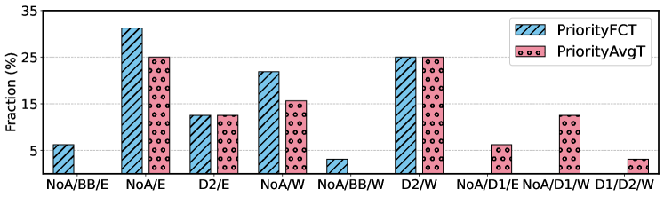
Figure 7. SWARM’s actions in Scenario 1 (see §4): it chooses from nine action combinations, while choosing no action more than 35% of the time. The action encoding is as follows: NoA: No Action on link 2, D2: Disable link 2, BB: Bring Back link 1, D1: Disable link 1, W: WCMP Routing, E: ECMP Routing.

Figure 8 compares the performance penalty of SWARM to the various NetPilot variants for both comparators, across both failure patterns. SWARM achieves consistently low penalty for its target CLP metric: 99p FCT in Figure 8(a) and average throughput in Figure 8(b). Figure 8 demonstrates that, because NetPilot assumes the rest of the network is under-utilized, it aggressively shuts down links and causes a large performance impact. Under PriorityFCT, SWARM chooses a mitigation with near optimal performance on FCT, while NetPilot, the next best approach, suffers a FCT penalty of 38%. Under the PriorityAvgT comparator, the NetPilot-80/99 variants result in lower impact on average throughput, but at the cost of increased performance penalty in at least one other metric (e.g., NetPilot-80 achieves $7.2\%$ less penalty in terms of average throughput at the cost of $\leavevmode\nobreak\ 80\%$ penalty on $99$p FCT) while SWARM is the only technique that performs well across both comparators and all three metrics.

Scenario 3: Packet corruption at ToR. In this scenario, we consider (Table A.1) failure patterns where each of the ToR and core links have both high O($10^{-2}$) and low O($10^{-5}$) packet drop rates, as well as those where the core link has no packet loss (a ToR-only failure). CorrOpt and NetPilot cannot mitigate this type of failure; they can only account for scenarios where the network has redundant paths. The operator playbook makes a local decision on whether to mitigate the failure based on severity of the packet loss, which ignores the conditions in the rest of the network. If a second failure occurs above the ToR, it reduces capacity in the network core and the operator’s approach breaks down which results in high performance penalties.

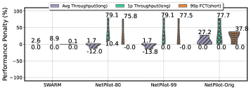
(a) PriorityFCT

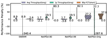
(b) PriorityAvgT

Figure 8. Comparison of SWARM and NetPilot variants under Scenario 2. Under the PriorityFCT comparator, SWARM always chooses a mitigation that provides near-optimal performance on FCT ($\leq$ 0.1%), while NetPilot, the next best approach, chooses mitigations up to 37.8% worse than optimal. For PriorityAvgT, SWARM performs similar to the NetPilot-80/99 variants in terms of Avg Throughput and is the only approach achieving low performance penalty across all three metrics.

The playbook-based approaches, with different thresholds, both suffer from performance penalties at least 2$\times$ higher than SWARM under PriorityFCT (Figure 9). SWARM has a worst-case FCT penalty of 28.9% while the best operator approach Operator-25 has a worst-case FCT penalty of 57%. Once again, SWARM is the only approach that achieves low penalty across all three metrics for both comparators.

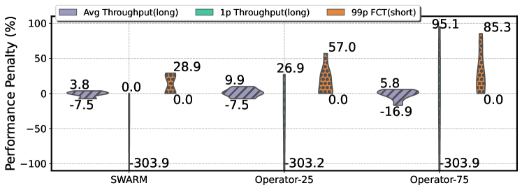
(a) Priority FCT

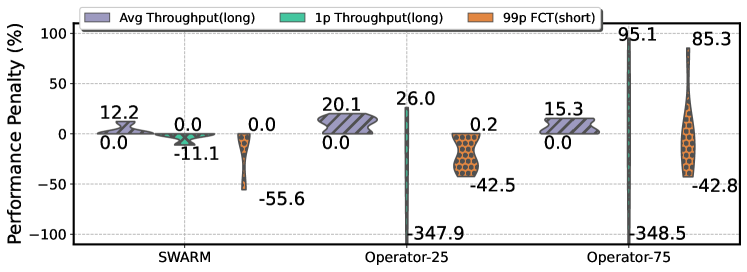
(b) Priority AvgT

Figure 9. Comparison of SWARM and operator playbooks on Scenario 3. Under PriorityFCT, SWARM outperforms operator playbooks by at least 2x in 99p FCT in the worst case while protecting the other two metrics. It is consistently able to protect other non-priority metrics while optimizing for the priority metric (e.g., it outperforms baselines in 99% FCT under PriorityAvgT while also reducing impact on average throughput).

4.3. Other Results

Scalability. SWARM scales (Figure 11(a)) to large Clos topologies with up to $16$K servers: for these, it can find the best mitigation in less than $5$ minutes, a small fraction of the mitigation times operators report today (GCP, [n. d.]; Gao et al., 2020).

SWARM scales without sacrificing accuracy (Figure 11(b)). Each technique in §3.4 contributes significantly: (a) the max-min fair algorithm improves run-time by $36.3\times$ and only introduces $\leq 0.9\%$ error; (b) down-scaling traffic by an additional $2\times$ does not introduce additional error but produces $73.6\times$ speedup! (c) adding warm-start and reducing the number of epochs results in $105.7\times$ speedup and $\leq 1.2\%$ error. Increasing the scale factor or reducing the number of epochs can increase speedup; we leave this to future work.

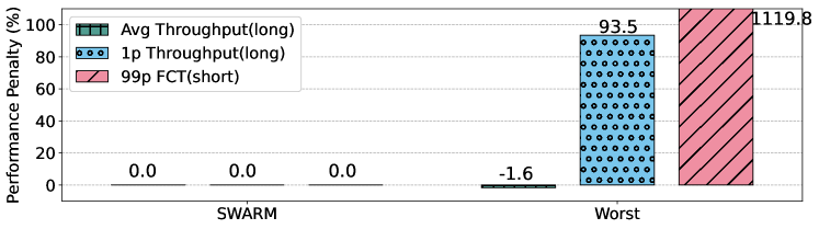
(a) Priority FCT

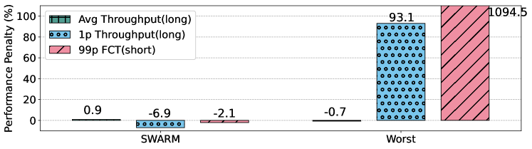
(b) Priority AvgT

Figure 10. Validation of SWARM on a physical testbed.

Sensitivity analysis. We evaluated SWARM’s sensitivity to various inputs including the packet drop rate estimates, and flow-arrival rates, and uncertainty in the input traffic distributions (see §D.1 in the appendix for details).

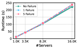
(a) Runtime for different topology sizes

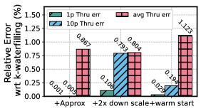
(b) Estimation Error for different scalability choices

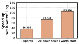
(c) Speed up for different scalability choices

Figure 11. Scalability. (a) SWARM scales almost linearly with the number of servers. (b) Accuracy sacrificed for achieving scale (approx refers to the ultra-fast max-min fair algorithm). (c) Speed-up from each of our scaling components. Here, we use extended k-waterfilling (Jose et al., 2019) (k=$1$) as the baseline for computing max-min fair rates.

Outside of a few inflection points the choice of what mitigation is best is clear: as the inputs to the system vary, there are only few inflection points where SWARM is sensitive to errors in the inputs. These points are where SWARM can make mistakes and pick sub-optimal mitigations if the inputs are noisy. But we find the difference between the performance penalty of the mitigations is small around these inputs. Outside of these areas the choice of the better mitigation is clear. Thus, SWARM can tolerate large error in the input distribution: the difference between mitigations is either large enough around that point so the choice of mitigation is clear or it is small enough where a mistake is not too costly.

SWARM is able to pick the best mitigation under different congestion control protocols (see Figure A.3). For this, we compare two protocols with different behaviors under loss: Cubic (Ha et al., 2008), which drastically reduces its sending rate when it observes packet loss, and BBR (Cardwell et al., 2016) which does not. SWARM picks the best mitigation irrespective of which protocol we use. But its approximations of the $1$p throughput distribution are more accurate when the mix of protocols is known (it can explicitly account for their differences in handling loss).

Testbed validation. To demonstrate that SWARM makes high-quality mitigation decisions even on a physical testbed, we induce a failure pattern from Scenario 1 in which a link from a TOR to T1 randomly drops packets at a rate 6.25% (1/16 packets), while a link from a different T1 to a T2 also drops packets at 0.39% (1/256 packets). SWARM picks an optimal mitigation for Priority-FCT, and picks a mitigation with less than 1% performance penalty for PriorityAvgT (Figure 10). In contrast, the FCT performance penalty from choosing the worst action under PriorityFCT is over 1000%. While the average throughput performance penalty is low across all mitigations in this incident, under the PriorityAvgT comparator SWARM picks an action with low penalty across all three metrics, avoiding the 93% penalty to 1p throughput and 1095% penalty to 99p FCT of the worst action.

We conclude that SWARM chooses the optimal or near-optimal mitigation both on the wide range of emulated incidents evaluated in Mininet, as well as on a real incident in a physical network, avoiding orders of magnitude of unnecessary performance loss from a poor mitigation.

Justifying design choices. We also conducted several experiments to justify: special treatment of loss-limited flows; estimating distributions of FCT and throughput; using multiple epochs to capture flow dynamics; using distributional measures to determine the best mitigation; and the importance of accounting for queueing delay (see §D.2).

5. Discussion and Limitations

SWARM is a first step towards CLP-aware incident mitigation. It has limitations that future work can address.

Support for loss-less transport. Cloud providers increasingly use RDMA (Gao et al., 2021; Singhvi et al., 2020) for internal traffic. We can modify SWARM’s CLPEstimator to (a) detect and account for pauses and (b) when losses happen, model loss-recovery approaches.

Mitigations with transient effects. Some actions introduce transient risk. For example, a switch drops packets during reboot. SWARM needs to account for this, since a reboot can induce non-steady-state behavior on long flows.

Approximate failure localization. SWARM waits for operators or automation to localize the failure. It can instead use a spatial failure distribution which is available much sooner. This lowers the mean time to repair. SWARM relies on the correct input of the type of failure.

Impact on wide area network traffic. WAN traffic is a small fraction of data center traffic (Firestone et al., 2018; Benson et al., 2010), so we ignore its impact. When WAN traffic increases, we would need to account its larger RTT.

Other extensions. Future work can extend SWARM to other metrics such as jitter, and failures of software components such as load balancers. It can also account for estimated repair time in ranking mitigations; this can be challenging because incidents that have vastly different repair times often have similar symptoms (Govindan et al., 2016).

6. Related Work

Impact or risk estimation in networking. No prior work considers CLP-aware failure mitigation but several estimate the impact or future risk of management operations. Janus (Alipourfard et al., 2019) focuses on risk estimation for DC management operations; RSS (Xia et al., 2021) estimates risk for backbone management; TEAVAR (Bogle et al., 2019) and (Dikbiyik et al., 2014; Vidalenc et al., 2013) route traffic in production wide area networks to minimize long-term impact; and (Mitra and Wang, 2005) models the risk of demand uncertainty and its impact on revenue in a WAN. Other approaches minimize the impact of failures without explicitly accounting for risk (Liu et al., 2014; Zhong et al., 2021).

NetPilot (Wu et al., 2012) and CorrOpt (Zhuo et al., 2017) are closest to SWARM. These can fail to produce mitigations with minimal CLP impact (see §2) because they: (a) ignore the failure pattern; (b) do not account for changes in traffic after they mitigate; (c) use proxy metrics (e.g., maximum utilization), that only loosely correlate with CLPs, to quantify impact; and (d) estimate impact on a healthy network, which makes it difficult to analyze the impact of undoing previous mitigations.

Computing fair share. Prior work assumes flows follow max-min fairness, which matches the objective of TCP (Fred et al., 2001), and either employ optimization (Singla et al., 2012; Namyar et al., 2021; Hong et al., 2013; Danna et al., 2012), use simulations (Zhao et al., 2022), or iterative algorithms (Jose et al., 2019; Jain et al., 2013; Ros-Giralt et al., 2021; Danna et al., 2017; Ros-Giralt and Tsai, 2001) to find the fair share. These approaches are limited; they either focus on throughput-limited flows or assume flow rates are only limited by the network capacity and ignore packet drops.

7. Conclusion

While failure mitigations are crucial to running a DC network at scale, operators often find it hard to choose the right mitigation. SWARM ranks mitigations based on their impact on well-known CLP metrics. Our evaluation shows the careful modeling of these objectives pays off: SWARM is significantly more robust than both existing operator playbooks and state-of-the-art systems: in the most common scenario, SWARM reduces the performance penalty, for a p99 FCT objective, by 793$\times$ over the next best system.

Appendix A Algorithm details

A.1. Details of the CLPEstimator function

Algorithm 2 shows the CLPEstimator in detail. The impact estimator first computes the number of samples it needs for a given confidence threshold based on (Dvoretzky et al., 1956). It then updates the topology and the traffic based on the mitigation $\mathcal{M}$. Finally, it divides the updated traffic into short and long flows, and compute their CLPs separately (§3.3).

Input: $\mathcal{T}$. traffic matrix {$<$src, dst, start time, size$>$}.

Input: $G$. current network state (location, type, and magnitude of failures).

Input: $\mathcal{M}$. mitigation.

Input: $\alpha$. confidence threshold

Output: $\beta_{l}$ = $\{<\beta_{l}^{\mathcal{S(P)}},\mathcal{S(P)}.prob>\}$. For all possible combination of flow paths $\mathcal{S(P)}$, $\beta_{l}^{,\mathcal{S(P)}}$ is the distribution of impact over all long flows.

Output: $\beta_{s}$ = $\{<\beta_{s}^{\mathcal{S(P)}},\mathcal{S(P)}.prob>\}$. For all possible combination of flow paths $\mathcal{S(P)}$, $\beta_{s}^{\mathcal{S(P)}}$ is the distribution of impact over all short flows.

1 $N\leftarrow num\_samples(\alpha)$

2 $G_{a},\mathcal{T}_{a}\leftarrow apply\_mitigation(G,\mathcal{M},\mathcal{T})$

3 $\mathcal{T}_{s},\mathcal{T}_{l}\leftarrow split\_traffic(\mathcal{T}_{a})$

4 for $n\in 1\dots N$ do

5       $\mathcal{P}_{n}\leftarrow get\_sample(\mathcal{S(P)})$

6       $\beta_{l}^{\mathcal{P}_{n}}\leftarrow impact\_long\_flows(G_{a},\mathcal{T}_{l},\mathcal{P}_{n})$

7       $\beta_{s}^{\mathcal{P}_{n}}\leftarrow impact\_short\_flows(G_{a},\mathcal{T}_{s},\mathcal{P}_{n})$

8      

9 end for

return $\beta_{l}$, $\beta_{s}$

Algorithm 2 CLPEstimator Function.

A.2. Demand-Aware Max-Min Fair

This section describes how we compute the max-min fair rate of flows given their drop-limited throughput. (Algorithm 4, Line 4). Algorithms to compute max-min fairness (Jose et al., 2019) assume demands are unbounded and are only limited by the network capacities. In SWARM, when we account for drop-limited flows we assume there is no congestion and so we find the maximum rate they can achieve using the packet drop rate on their route. We then model these drop-based rates in the max-min fair throughput computation by adding one virtual edge per flow with capacity = drop-based rate. This ensures the flow would not get more than its drop-based throughput, and at the same time, if congestion is more severe than the drop rate, the flow would be limited by its fair share. We can use the same method to model congestion control rate limits in the first few epochs of each flow. For example, scenarios where the protocol’s congestion window limits a flow’s rate.

We can use any of the variants of the k-waterfilling algorithm (Jose et al., 2019) in the network-wide-max-min-fair function in Line 3 (but some can result in O(|E| + |F|) number of iterations where |E| is the number of edges and |F| the number of flows).

We instead use a faster variant of max-min fairness that improves the speed up of k-waterfilling by 30x with minor degradation in the quality of the estimated metric (Figure 11(c), Figure 11(b)).

Input: $G$. current network state.

Input: $\mathcal{T}_{1\times M}$. source destination pairs (long flows).

Input: $\mathcal{P}_{1\times M}$. The (sampled) paths for each flow.

Input: $\theta_{1\times M}$. Input demand rate (=drop-limited rate) for all the flows.

Output: $\hat{\theta}_{1\times M}$. The max-min fair throughput rates after applying congestion.

1 for $\forall f\in\mathcal{T}$ do

       /* add one virtual edge to enforce demand per flow */

2       $e\leftarrow G.add\_virtual\_edge()$

       /* set the capacity of the link to the drop-limited rate */

3       $e.capacity=\theta_{f}$

       /* add the new link to the route of flow $f$ */

4       $\mathcal{P}_{f}.add(e)$

5      

6 end for

7$\hat{\theta}\leftarrow network\_wide\_max\_min\_fairness(G,\mathcal{T},\mathcal{P})$

return $\hat{\theta}$

Algorithm 3 Demand-Aware Max-Min Fair.

Input: $G$. current network state.

Input: $\mathcal{T}_{1\times n}$. source destination pairs (long flows).

Input: $\mathcal{P}_{1\times n}$. The (sampled) paths for each flow.

Output: $F$. Max-Min Fair Throughput

1 $\theta\leftarrow get\_drop\_limited\_tput(G,\mathcal{T},\mathcal{P})$

2

3$F\leftarrow demand\_aware\_max\_min\_fair(G,\mathcal{T},\theta,\mathcal{P})$

return F

Algorithm 4 Compute throughput.

Appendix B Details of offline measurements

SWARM relies on three empirically driven distributions that we measure offline: the upper bound on the throughput of long flows in a lossy network, the number of RTTs needed for short flows to complete and their queueing delay. In this section, we describe how we gathered these distributions in SWARM. We also show a sample distribution in Figure A.8.

Throughput of long flows in a lossy network. We use the topology in Figure 1(a) where h1 sends a long flow, $f$, to h2. We measure the throughput of $f$ using iperf3 under different network conditions (e.g., by inducing packet drops in s1 – s2 or changing the RTT by adding delay on s1 – s2). We use link capacities high enough so flow $f$ is always bottlenecked by the drop rate: we use the throughput of a flow in a loss-less network as our baseline — if the flow’s throughput in a lossy network is less than this baseline we assume it is bottlenecked by the loss. We also repeat each experiment multiple times to create a statistically significant distribution (Dvoretzky et al., 1956).

Number of RTTs for short flows. Here we generate short flows between h1 and h2 in the same topology (Figure 1(a)). We measure the FCT of the flow under different flow (e.g., flow size, slow start threshold, initial congestion window) and network (e.g., packet drop rate, RTT) conditions. This gives us an FCT distribution. We divide this distribution by the two-way propagation delay of our setup (we only have one flow in this set up and so we can ignore queueing delay) to find the distribution of the number of RTTs we need to complete a flow. We also repeat each scenario multiple times to ensure the empirical distributions are statistically significant.

Queueing delay for short flows. It is harder to measure the queueing delay because it depends on competing traffic (e.g., the number of flows on the same bottleneck link).

We use the topology in Figure 1(b) to estimate a queueing delay distribution under various network conditions. We route $M$ long flows from h4 to h3, and $N$ additional flows from h4 to h5. Once these flows reach steady state, we route a small flow (that finishes within an RTT) between h1 and h3.

In the above scheme, the value $M+N$ controls the utilization on the s1 – s2 link (the $M$ long flows on the h4 – s1 link cause some flows to be bottlenecked before reaching s1 —s2) and $N$ controls the number of flows that compete on the link. To generate the FCT distributions that result from long flows competing on the links in our network we can vary both $M$ and $N$ to model different utilizations. We subtract the two way propagation delay of the flow from the FCT distribution to derive the queing delay distribution. Once again we repeat these experiments such that the resulting distributions are statistically significant.

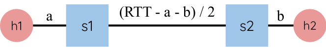
(a) Topology 1

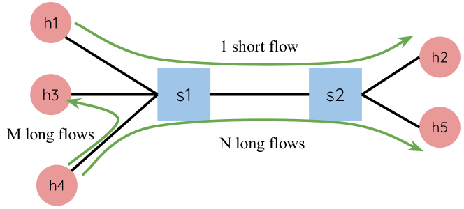
(b) Topology 2

Figure A.1. Topologies for offline measurements.

Appendix C Additional Experiment Details

Mininet. For all the Mininet experiments unless mentioned otherwise, we use 30 different random traffic matrices, each 500s long. We compute CLP metrics on the flows that started within [50, 150) seconds.

SWARM. For all of our SWARM experiments (unless mentioned otherwise) we use 32 different, randomly generated, traffic matrices. Along with each traffic matrix we use 1000 different random routing samples. Each demand is 200s, and as in Mininet we compute the CLP metrics over all the flows that start within [50, 150) seconds. We also use 200 ms as the epoch size for Algorithm 1.

Scenarios. Table A.1 summarizes the details of all the failure scenarios we used to evaluate SWARM. In total, we evaluated 57 different cases, spanning across 3 failure scenarios.

		Details	#scenarios
Scen. 1	1 link failure	One T0 – T1 and one T1 –T2, each with two levels of packet drop rate O($10^{-2}$) and O($10^{-5}$)	4
	2 link failures	Four combination of pair of links (two T0 – T1s in the same cluster connected to the same T0, two T0 – T1s in the same cluster connected to different T0s & T1s, one T0 – T1 & one T1 – T2 connected to different T1s, and two T1 – T2s connected to different T1s & T2s), each with all combinations of the two packet drop levels and all the possible ordering of failures.	32
Scen. 2	no other link failure	one T1 – T2 with capacity reduced to half	1
	1 other link failure	one T1 – T2 with capacity reduced to half, another T0 –T1 link with 3 levels of failure (two packet drop levels + completely down), and all possible ordering of failures.	6
Scen. 3	no link failure	One T0 with two levels of packet drop rate O($10^{-2}$) and O($10^{-5}$)	2
	1 link failure	One T0 and One T0 – T1 in the same cluster connected to a different T0, with all combination of packet drop rates (ToR with two levels of packet drop rate and link with three levels of failure (two packet drop rates + completely down)), and all the possible ordering of failures.	12
		total number of evaluated scenarios	57

Table A.1. Mininet Experiment Details.

Appendix D Extended evaluation

In this section we present an extended evaluation of SWARM.

D.1. Sensitivity Analysis

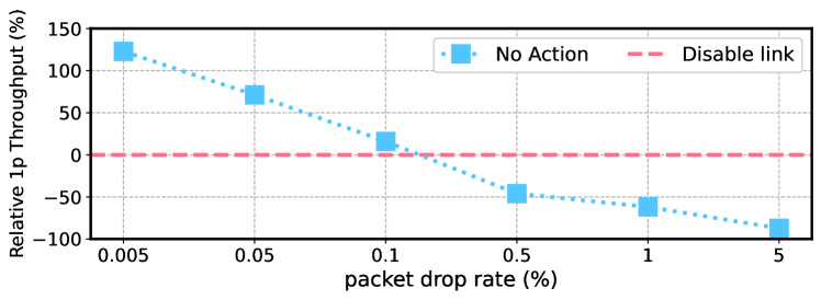
(a) Sensitivity to packet drop rate

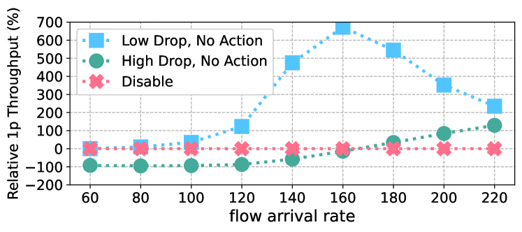
(b) Sensitivity to flow arrival rate changes

Figure A.2. Sensitivity Analysis. All experiments are in a scenario where a T0 – T1 drop packets. (a) shows the sensitivity to changes to the packet drop rate; (b) shows the sensitivity to errors in the input flow-arrival rate distribution under two different loss rates.

Next, we evaluate SWARM’s sensitivity to various design choices (Figure A.2).

Packet drop rates. To evaluate SWARM’s sensitivity to packet drop rates we consider a failure pattern in which a T0 – T1 link drops packets. Figure 2(a) shows the relative difference between the 1p throughput when we take no action vs when we disable the link under different drop rates (in log-scale). We find the choice of the right decision to be bi-modal with a wide room for error: for all drop rates below $\sim 0.1\%$ it is better to take no action while beyond that point the best action is to disable the link. Furthermore, the penalty close to this transition point ($0.1\%$ drop rate) is rather small. Put differently, the error in the input packet loss rate has to be an order of magnitude in order for SWARM to make the wrong decision, an unlikely possibility in today’s clouds.

Flow arrival rates. SWARM is resilient to small errors in the input flow arrival rate (Figure 2(b)). To show this, we investigate how SWARM’s decisions change with changing flow-arrival rates and under two different failure severities. We observe there are inflection points, outside of which the gap between the two decisions is significant which means SWARM will pick the best mitigation in most cases.

To see this, take the example of low drop rates where the difference between disabling the link and taking no action initially increases as arrival rates increase (120 – 160 fps): if we disable the link congestion will increase. Once we pass $160$ fps if we bring the link down we will fully congest the network and the difference shrinks. This means SWARM has a wide margin of error: for medium and large rates the difference between the two actions is consistently significant (we will always pick the right action) and at lower rates the difference is very small (whichever action we pick results in the same impact). We observe a similar behavior under the high drop rate scenario.

Sensitivity to the choice of Congestion Control. We conduct a limited experiment to evaluate whether SWARM is resilient to the choice of congestion control. We consider a scenario where a T0 – T1 and a T1 – T2 are dropping packets at low and high drop rates respectively. We use two example congestion control protocols i.e., CUBIC (Ha et al., 2008) and BBR (Cardwell et al., 2016): the two behave differently under loss — Cubic significantly reduces its rate under loss while BBR does not.

We compare SWARM’s estimated 1p throughput with what we observe in Mininet (Figure A.3) under four mitigations. We find SWARM is able to estimate throughput adequately enough to pick the best mitigation: the choice of the best action remains independent of the congestion control protocol being used with a large margin of error compared to the next best mitigation. We see, SWARM’s estimate is more accurate when it operates on the same congestion control protocol which is used by Mininet. This shows SWARM will be more robust if operators input the right probability distribution for how likely it is for different protocols to be used inside their DCs.

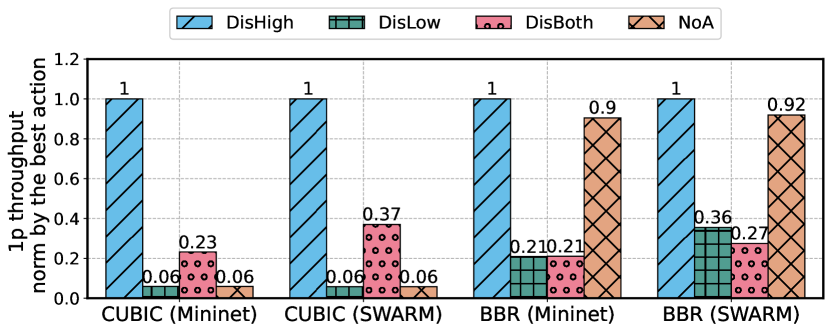
Figure A.3. Evaluation of SWARM on multiple congestion controls. In general, SWARM is able to correctly order the mitigation actions and approximately capture the relative difference between different mitigation actions on both congestion controls (BBR (Cardwell et al., 2016) and Cubic (Ha et al., 2008)).

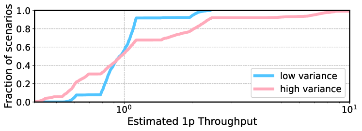
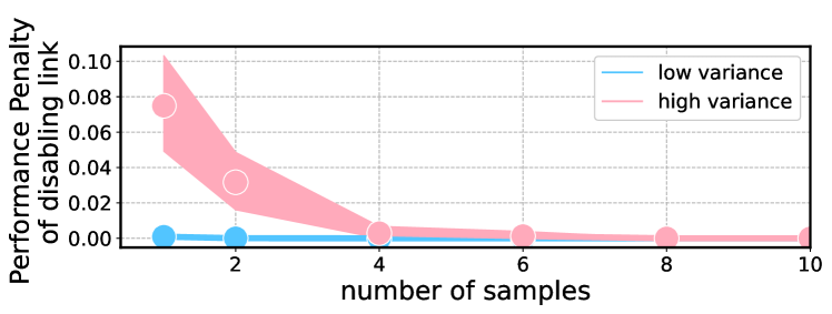
Figure A.4. Variance in the input flow arrival rate and it’s impact on the performance penalty of mitigation actions.

D.2. Validating assumptions and design choices

We also evaluate the underlying components and the assumptions we used in our design

Capturing the impact of drop-limited flows. SWARM has to account for drop-limited flows: we assume we can account for drop-limited flows by computing an upper bound on their achievable rate and then approximating the demand-constrained max-min fair rates under these constraints. Figure 5(a) shows this assumption is reasonable in an experiment where we use a single link that has varying packet-drop rates and a mixture of number of flows going over it.

We indeed observe flows are limited by their fair share rate when the drop rate is low and as the drop rate increases they become bottlenecked by the drop rate.

We next evaluate our design choices for estimating the distribution of the flow completion time and throughput (Figure 5(b)). Specifically, we show the quality of SWARM’s approximations compared to what we measure in Mininet. Here we use the scenario where two links drop packets at different rates and where the mitigation is to disable the link with the higher packet drop rate. The design choices we evaluate are:

Single Epoch vs. Multiple Epochs. In SWARM we use epochs to account for flow arrivals and departures which in turn cause changes in the available bandwidth: a single epoch assumed the set of flows a given flow has to compete with on the bottleneck link is not going to change throughout its lifetime. We see using a single epoch results in significant estimation error (more than 50% on average) which we can eliminate by switching to the multi-epoch approach.

Distributions vs deterministic estimates. SWARM relies on distributions to pick the best mitigation. We find if we switch to a single approximation (single sample) of throughout and flow completion time SWARM suffers. SWARM can generate these distributions (multiple samples) efficiently as it can generate different samples in parallel.

Queueing Delay. Finally we show it is important to account for queuing delay. To do so, we use an example scenario where link C0 – B0 in topology Figure 1 drops packets at a high drop rate and the operator prioritizes 99p FCT. The best action here is to disable the link but after we apply this mitigation the link C0 – B1 starts to drop packets at a high drop rate as well. Unfortunately, if we disable C0 – B1, we would have a network partition.

In this setup, and when we ignore queuing delay, the approximate 99p FCT is the same if we bring back C0 – B1 and if we take no action. But bringing back C0 – B1 is actually the better mitigation as it reduces queuing delay. We compare the effect of these mitigations in Table 2(a).

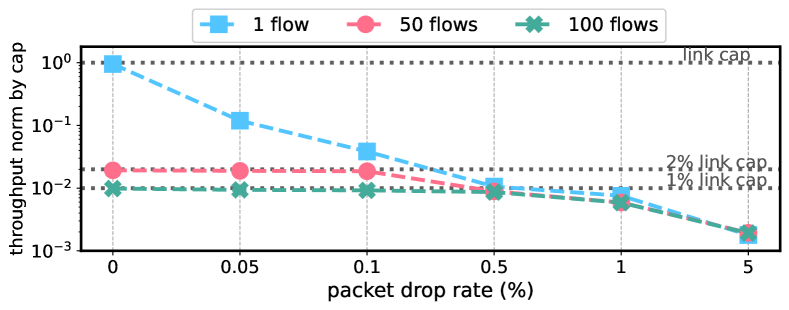
(a) Drop-limited vs Capacity-limited

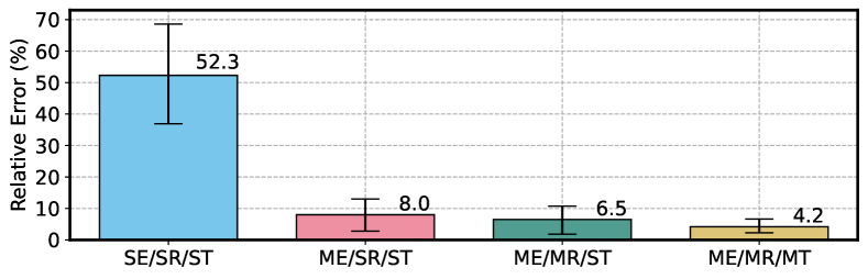
(b) Impact of different design choices on throughput estimation (E=Epoch, R=Routing Sample, T=Traffic Sample, S=Single, M=Multiple). For example, SE/SR/ST refers to using a single epoch, with a single routing sample, and a single traffic sample. We run each method with 10 different seeds.

Approach	Best Action	FCT Penalty
Ignore Queueing	Disable C0 – B0	48 %
Model Queueing	Bring back C0 – B0	0 %

(a) How queueing delay influences the mitigation choice.

Figure A.5. Validationg assumptions and design choices. (a) shows when flows are capacity vs loss limited — when the throughput of a group of flows drops below their corresponding fair share of the link capacity (marked as dashed lines) the flow is loss limited. (b) shows the impact of the various speed up techniques we use and the relative error they introduce: the combination of these techniques both reduces the error and results in significant speedup. (c) the importance of accounting for queuing delay.

D.3. Results for other comparators

Priority1pT. This comparator minimizes the 1p ($1$-th percentile) throughput. It uses two tiebreakers, in the following order: average throughput and 99p FCT.

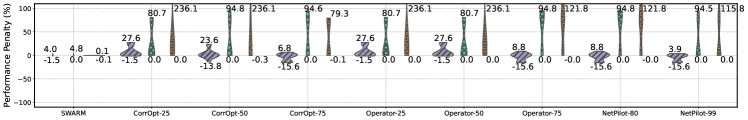
() Scenario 1

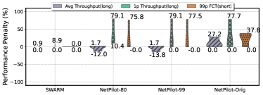
(a) Scenario 2

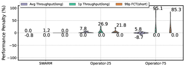
(b) Scenario 3

Figure A.6. Priority1pT: Comparing the performance penalty of SWARM to baselines under Priority1pT comparator.. SWARM outperforms all the other baselines (for example, by 16.8x on the most prefered metric in Scenario 1) and it is the only method that achieves consistently low performance penalty across all the metric and all the scenarios.

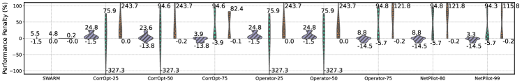
() Scenario 1

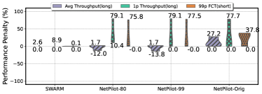
(a) Scenario 2

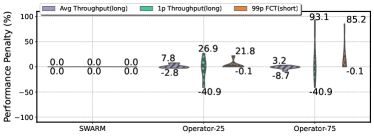
(b) Scenario 3

Figure A.7. Linear combination: Comparing the performance penalty of SWARM to baselines. SWARM achieves consistently low performance penalty (always $\leq$ 8.9%) accross all the three metrics and all the three scenarios.

Linear combination. This comparator minimizes a weighted combination of the three CLP metrics (i.e., 99p FCT, 1p throughput, and average throughput);

$$w_{0}\frac{99p\leavevmode\nobreak\ FCT}{99p\leavevmode\nobreak\ FCT_{h}}+w_{1}\frac{1p\leavevmode\nobreak\ Thru_{h}}{1p\leavevmode\nobreak\ Thru}+w_{2}\frac{avg\leavevmode\nobreak\ Thru_{h}}{avg\leavevmode\nobreak\ Thru}$$

where $w_{i}$s’ show the weights assigned to each metric and $Metric_{h}$ shows the measured metric when the network was healthy. Note that 1p throughput and average throughput move in the opposite direction compared to FCT (i.e., we prefer a lower FCT while we prefer higher throughput). Therefore, we use inverse of them in our definition of linear comparator. Figure A.7 shows the results when the weights = 1 (i.e., we do not have any preference over the metrics – we choose these weights because it is substantially different from all the other comparators but SWARM admits any combination of weights).

Summary of the results. Figure A.7 and Figure A.7 compare the performance penalty of SWARM againts other baselines across 3 different failure scenarios for Priority1pT and Linear combination comparator respectively. In summary, we observe SWARM’s performance penalty is low across various scenarios and metrics. The results are also generalizable to different comparators (we evaluate 4 different comparators in total including the two in the §4).

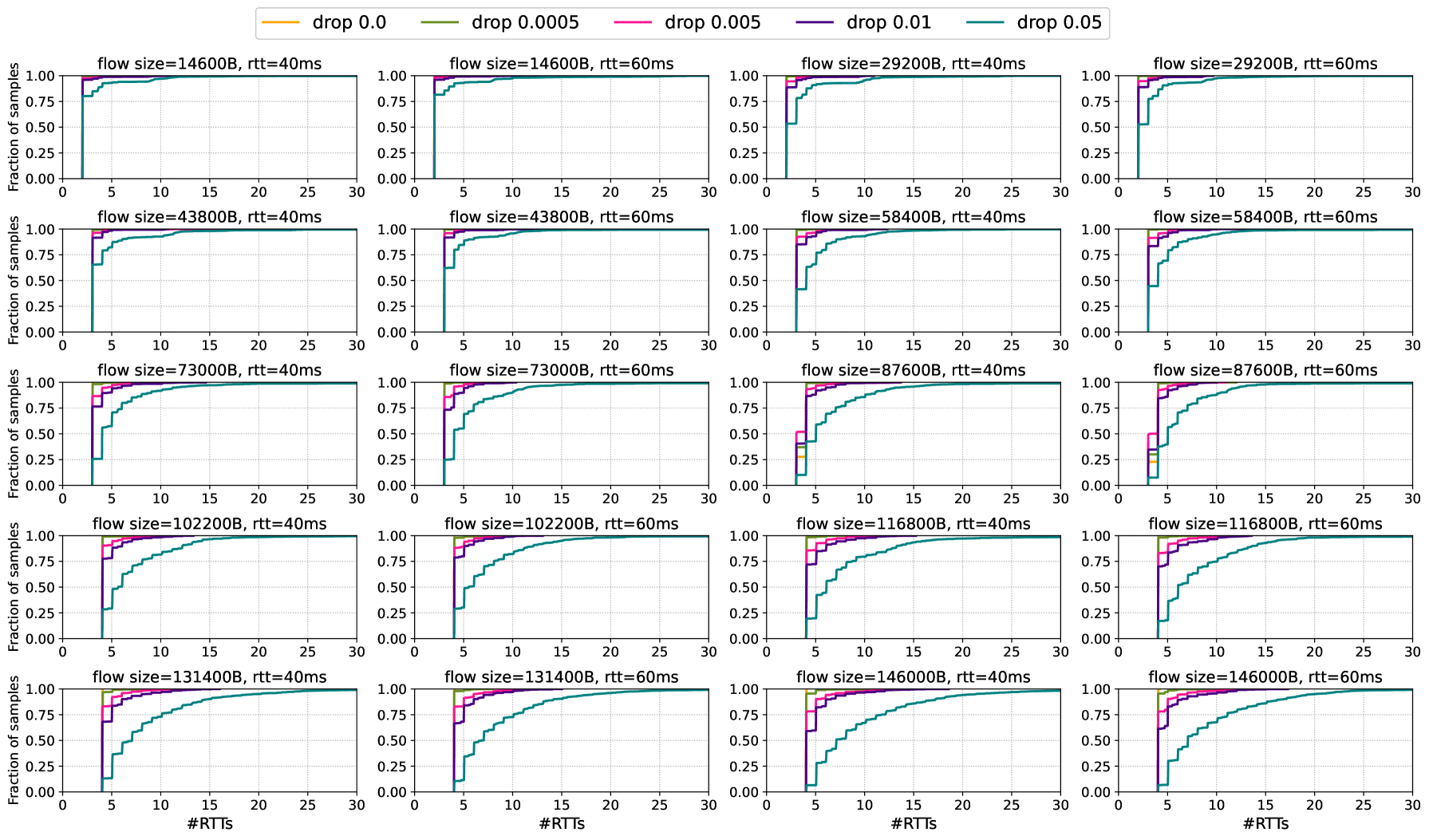
Figure A.8. An example of distribution measured for short flow’s FCT.

References

- (1)
- GCP ([n. d.]) [n. d.]. Google Cloud incident summary. https://status.cloud.google.com/summary. ([n. d.]).
- Azu ([n. d.]) [n. d.]. RCA - Network Latency Issue – West Europe (Tracking ID 8KLC-1T8). https://status.azure.com/en-us/status/history/. ([n. d.]).
- max ([n. d.]) [n. d.]. Under submission. Details omitted for double-blind reviewing. ([n. d.]).
- Alipourfard et al. (2019) Omid Alipourfard, Jiaqi Gao, Jeremie Koenig, Chris Harshaw, Amin Vahdat, and Minlan Yu. 2019. Risk Based Planning of Network Changes in Evolving Data Centers. In Proceedings of the 27th ACM Symposium on Operating Systems Principles (SOSP ’19). Association for Computing Machinery, New York, NY, USA, 414–429. https://doi.org/10.1145/3341301.3359664
- Alizadeh et al. (2010) Mohammad Alizadeh, Albert Greenberg, David A. Maltz, Jitendra Padhye, Parveen Patel, Balaji Prabhakar, Sudipta Sengupta, and Murari Sridharan. 2010. Data Center TCP (DCTCP). In Proceedings of the ACM SIGCOMM 2010 Conference (SIGCOMM ’10). Association for Computing Machinery, New York, NY, USA, 63–74. https://doi.org/10.1145/1851182.1851192
- Arzani et al. (2018) Behnaz Arzani, Selim Ciraci, Luiz Chamon, Yibo Zhu, Hongqiang Harry Liu, Jitu Padhye, Boon Thau Loo, and Geoff Outhred. 2018. 007: Democratically finding the cause of packet drops. In 15th USENIX Symposium on Networked Systems Design and Implementation (NSDI 18). 419–435.
- Arzani et al. (2016) Behnaz Arzani, Selim Ciraci, Boon Thau Loo, Assaf Schuster, and Geoff Outhred. 2016. Taking the blame game out of data centers operations with netpoirot. In Proceedings of the 2016 ACM SIGCOMM Conference. 440–453.
- Arzani et al. (2020) Behnaz Arzani, Selim Ciraci, Stefan Saroiu, Alec Wolman, Jack Stokes, Geoff Outhred, and Lechao Diwu. 2020. Privateeye: Scalable and privacy-preserving compromise detection in the cloud. In 17th USENIX Symposium on Networked Systems Design and Implementation (NSDI 20). 797–815.
- Benson et al. (2010) Theophilus Benson, Aditya Akella, and David A Maltz. 2010. Network traffic characteristics of data centers in the wild. In Proceedings of the 10th ACM SIGCOMM conference on Internet measurement. 267–280.
- Bogle et al. (2019) Jeremy Bogle, Nikhil Bhatia, Manya Ghobadi, Ishai Menache, Nikolaj Bjørner, Asaf Valadarsky, and Michael Schapira. 2019. TEAVAR: Striking the Right Utilization-Availability Balance in WAN Traffic Engineering. In Proceedings of the ACM Special Interest Group on Data Communication (SIGCOMM ’19). Association for Computing Machinery, New York, NY, USA, 29–43. https://doi.org/10.1145/3341302.3342069
- Cardwell et al. (2016) Neal Cardwell, Yuchung Cheng, C. Stephen Gunn, Soheil Hassas Yeganeh, and Van Jacobson. 2016. BBR: Congestion-Based Congestion Control. ACM Queue 14, September-October (2016), 20 – 53. http://queue.acm.org/detail.cfm?id=3022184
- Case et al. (1989) Jeffrey D Case, Mark Fedor, Martin L Schoffstall, and James Davin. 1989. Simple network management protocol (SNMP). Technical Report.
- Cormode et al. (2012) Graham Cormode, Minos Garofalakis, Peter J. Haas, and Chris Jermaine. 2012. Synopses for Massive Data: Samples, Histograms, Wavelets, Sketches. Found. Trends Databases 4, 1–3 (jan 2012), 1–294. https://doi.org/10.1561/1900000004
- Danna et al. (2017) Emilie Danna, Avinatan Hassidim, Haim Kaplan, Alok Kumar, Yishay Mansour, Danny Raz, and Michal Segalov. 2017. Upward Max-Min Fairness. J. ACM 64, 1, Article 2 (mar 2017), 24 pages. https://doi.org/10.1145/3011282
- Danna et al. (2012) Emilie Danna, Subhasree Mandal, and Arjun Singh. 2012. A practical algorithm for balancing the max-min fairness and throughput objectives in traffic engineering. In 2012 Proceedings IEEE INFOCOM. 846–854. https://doi.org/10.1109/INFCOM.2012.6195833
- Dikbiyik et al. (2014) Ferhat Dikbiyik, Massimo Tornatore, and Biswanath Mukherjee. 2014. Minimizing the Risk From Disaster Failures in Optical Backbone Networks. Journal of Lightwave Technology 32, 18 (2014), 3175–3183. https://doi.org/10.1109/JLT.2014.2334713
- Dvoretzky et al. (1956) A. Dvoretzky, J. Kiefer, and J. Wolfowitz. 1956. Asymptotic Minimax Character of the Sample Distribution Function and of the Classical Multinomial Estimator. The Annals of Mathematical Statistics 27, 3 (1956), 642 – 669. https://doi.org/10.1214/aoms/1177728174
- Firestone et al. (2018) Daniel Firestone, Andrew Putnam, Sambhrama Mundkur, Derek Chiou, Alireza Dabagh, Mike Andrewartha, Hari Angepat, Vivek Bhanu, Adrian Caulfield, Eric Chung, et al. 2018. Azure Accelerated Networking:SmartNICs in the Public Cloud. In USENIX Symposium on Networked Systems Design and Implementation. 51–66.
- Fred et al. (2001) S. Ben Fred, T. Bonald, A. Proutiere, G. Régnié, and J. W. Roberts. 2001. Statistical Bandwidth Sharing: A Study of Congestion at Flow Level. In Proceedings of the 2001 Conference on Applications, Technologies, Architectures, and Protocols for Computer Communications (SIGCOMM ’01). Association for Computing Machinery, New York, NY, USA, 111–122. https://doi.org/10.1145/383059.383068
- Gao et al. (2020) Jiaqi Gao, Nofel Yaseen, Robert MacDavid, Felipe Vieira Frujeri, Vincent Liu, Ricardo Bianchini, Ramaswamy Aditya, Xiaohang Wang, Henry Lee, David Maltz, et al. 2020. Scouts: Improving the diagnosis process through domain-customized incident routing. In Proceedings of the Annual conference of the ACM Special Interest Group on Data Communication on the applications, technologies, architectures, and protocols for computer communication. 253–269.
- Gao et al. (2021) Yixiao Gao, Qiang Li, Lingbo Tang, Yongqing Xi, Pengcheng Zhang, Wenwen Peng, Bo Li, Yaohui Wu, Shaozong Liu, Lei Yan, et al. 2021. When Cloud Storage Meets RDMA. In 18th USENIX Symposium on Networked Systems Design and Implementation (NSDI 21). 519–533.
- Ghobadi et al. (2016) Monia Ghobadi, Ratul Mahajan, Amar Phanishayee, Nikhil Devanur, Janardhan Kulkarni, Gireeja Ranade, Pierre-Alexandre Blanche, Houman Rastegarfar, Madeleine Glick, and Daniel Kilper. 2016. ProjecToR: Agile Reconfigurable Data Center Interconnect. In Proceedings of the 2016 ACM SIGCOMM Conference (SIGCOMM ’16). Association for Computing Machinery, New York, NY, USA, 216–229. https://doi.org/10.1145/2934872.2934911
- Govindan et al. (2016) Ramesh Govindan, Ina Minei, Mahesh Kallahalla, Bikash Koley, and Amin Vahdat. 2016. Evolve or Die: High-Availability Design Principles Drawn from Googles Network Infrastructure. In Proceedings of the 2016 ACM SIGCOMM Conference (SIGCOMM ’16). Association for Computing Machinery, New York, NY, USA, 58–72. https://doi.org/10.1145/2934872.2934891
- Grandl et al. (2014) Robert Grandl, Ganesh Ananthanarayanan, Srikanth Kandula, Sriram Rao, and Aditya Akella. 2014. Multi-Resource Packing for Cluster Schedulers. In Proceedings of the 2014 ACM Conference on SIGCOMM (SIGCOMM ’14). Association for Computing Machinery, New York, NY, USA, 455–466. https://doi.org/10.1145/2619239.2626334
- Greenberg et al. (2009) Albert Greenberg, James R. Hamilton, Navendu Jain, Srikanth Kandula, Changhoon Kim, Parantap Lahiri, David A. Maltz, Parveen Patel, and Sudipta Sengupta. 2009. VL2: A Scalable and Flexible Data Center Network. In Proceedings of the ACM SIGCOMM 2009 Conference on Data Communication (SIGCOMM ’09). Association for Computing Machinery, New York, NY, USA, 51–62. https://doi.org/10.1145/1592568.1592576
- Ha et al. (2008) Sangtae Ha, Injong Rhee, and Lisong Xu. 2008. CUBIC: a new TCP-friendly high-speed TCP variant. ACM SIGOPS operating systems review 42, 5 (2008), 64–74.
- Henderson et al. (2008) Thomas R Henderson, Mathieu Lacage, George F Riley, Craig Dowell, and Joseph Kopena. 2008. Network simulations with the ns-3 simulator. SIGCOMM demonstration 14, 14 (2008), 527.
- Hong et al. (2013) Chi-Yao Hong, Srikanth Kandula, Ratul Mahajan, Ming Zhang, Vijay Gill, Mohan Nanduri, and Roger Wattenhofer. 2013. Achieving high utilization with software-driven WAN. In Proceedings of the ACM SIGCOMM 2013 Conference on SIGCOMM. 15–26.
- Huang et al. (2020) Qun Huang, Haifeng Sun, Patrick PC Lee, Wei Bai, Feng Zhu, and Yungang Bao. 2020. Omnimon: Re-architecting network telemetry with resource efficiency and full accuracy. In Proceedings of the Annual conference of the ACM Special Interest Group on Data Communication on the applications, technologies, architectures, and protocols for computer communication. 404–421.
- Jain et al. (2013) Sushant Jain, Alok Kumar, Subhasree Mandal, Joon Ong, Leon Poutievski, Arjun Singh, Subbaiah Venkata, Jim Wanderer, Junlan Zhou, Min Zhu, Jon Zolla, Urs Hölzle, Stephen Stuart, and Amin Vahdat. 2013. B4: Experience with a Globally-Deployed Software Defined Wan. In Proceedings of the ACM SIGCOMM 2013 Conference on SIGCOMM (SIGCOMM ’13). Association for Computing Machinery, New York, NY, USA, 3–14. https://doi.org/10.1145/2486001.2486019
- Jose et al. (2019) Lavanya Jose, Stephen Ibanez, Mohammad Alizadeh, and Nick McKeown. 2019. A distributed algorithm to calculate max-min fair rates without per-flow state. Proceedings of the ACM on Measurement and Analysis of Computing Systems 3, 2 (2019), 1–42.
- Kassing et al. (2017) Simon Kassing, Asaf Valadarsky, Gal Shahaf, Michael Schapira, and Ankit Singla. 2017. Beyond Fat-Trees without Antennae, Mirrors, and Disco-Balls. In Proceedings of the Conference of the ACM Special Interest Group on Data Communication (SIGCOMM ’17). Association for Computing Machinery, New York, NY, USA, 281–294. https://doi.org/10.1145/3098822.3098836
- Kelly (2003) Frank Kelly. 2003. Fairness and stability of end-to-end congestion control. European journal of control 9, 2-3 (2003), 159–176.
- Lantz et al. (2010) Bob Lantz, Brandon Heller, and Nick McKeown. 2010. A network in a laptop: rapid prototyping for software-defined networks. In ACM SIGCOMM Workshop on Hot Topics in Networks. 1–6.
- Liu et al. (2014) Hongqiang Harry Liu, Srikanth Kandula, Ratul Mahajan, Ming Zhang, and David Gelernter. 2014. Traffic engineering with forward fault correction. In Proceedings of the 2014 ACM Conference on SIGCOMM. 527–538.
- Lonvick (2001) Chris Lonvick. 2001. The BSD syslog protocol. Technical Report.
- Mellette et al. (2020) William M. Mellette, Rajdeep Das, Yibo Guo, Rob McGuinness, Alex C. Snoeren, and George Porter. 2020. Expanding across time to deliver bandwidth efficiency and low latency. In 17th USENIX Symposium on Networked Systems Design and Implementation (NSDI 20). USENIX Association, Santa Clara, CA, 1–18. https://www.usenix.org/conference/nsdi20/presentation/mellette
- Mellia and Zhang (2002) Marco Mellia and Hui Zhang. 2002. TCP model for short lived flows. IEEE communications letters 6, 2 (2002), 85–87.
- Mitra and Wang (2005) D. Mitra and Qiong Wang. 2005. Stochastic traffic engineering for demand uncertainty and risk-aware network revenue management. IEEE/ACM Transactions on Networking 13, 2 (2005), 221–233. https://doi.org/10.1109/TNET.2005.845527
- Montazeri et al. (2018) Behnam Montazeri, Yilong Li, Mohammad Alizadeh, and John Ousterhout. 2018. Homa: A receiver-driven low-latency transport protocol using network priorities. In Proceedings of the 2018 Conference of the ACM Special Interest Group on Data Communication. 221–235.
- Namyar et al. (2021) Pooria Namyar, Sucha Supittayapornpong, Mingyang Zhang, Minlan Yu, and Ramesh Govindan. 2021. A Throughput-Centric View of the Performance of Datacenter Topologies. In Proceedings of the 2021 ACM SIGCOMM 2021 Conference (SIGCOMM ’21). Association for Computing Machinery, New York, NY, USA, 349–369. https://doi.org/10.1145/3452296.3472913
- Narayanan et al. (2021) Deepak Narayanan, Fiodar Kazhamiaka, Firas Abuzaid, Peter Kraft, Akshay Agrawal, Srikanth Kandula, Stephen Boyd, and Matei Zaharia. 2021. Solving Large-Scale Granular Resource Allocation Problems Efficiently with POP (SOSP ’21). Association for Computing Machinery, New York, NY, USA, 521–537. https://doi.org/10.1145/3477132.3483588
- Robinson (2008) Derek W Robinson. 2008. Entropy and uncertainty. Entropy 10, 4 (2008), 493–506.
- Ros-Giralt et al. (2021) Jordi Ros-Giralt, Noah Amsel, Sruthi Yellamraju, James Ezick, Richard Lethin, Yuang Jiang, Aosong Feng, Leandros Tassiulas, Zhenguo Wu, Min Yee Teh, and Keren Bergman. 2021. Designing Data Center Networks Using Bottleneck Structures. In Proceedings of the 2021 ACM SIGCOMM 2021 Conference (SIGCOMM ’21). Association for Computing Machinery, New York, NY, USA, 319–348. https://doi.org/10.1145/3452296.3472898
- Ros-Giralt and Tsai (2001) Jordi Ros-Giralt and Wei Kang Tsai. 2001. A theory of convergence order of maxmin rate allocation and an optimal protocol. In Proceedings IEEE INFOCOM 2001. Conference on Computer Communications. Twentieth Annual Joint Conference of the IEEE Computer and Communications Society (Cat. No. 01CH37213), Vol. 2. IEEE, 717–726.
- Roy et al. (2017) Arjun Roy, Hongyi Zeng, Jasmeet Bagga, and Alex C Snoeren. 2017. Passive realtime datacenter fault detection and localization. In 14th USENIX Symposium on Networked Systems Design and Implementation (NSDI 17). 595–612.
- Sarykalin et al. (2008) Sergey Sarykalin, Gaia Serraino, and Stan Uryasev. 2008. Value-at-risk vs. conditional value-at-risk in risk management and optimization. In State-of-the-art decision-making tools in the information-intensive age. Informs, 270–294.
- Singh et al. (2015) Arjun Singh, Joon Ong, Amit Agarwal, Glen Anderson, Ashby Armistead, Roy Bannon, Seb Boving, Gaurav Desai, Bob Felderman, Paulie Germano, Anand Kanagala, Jeff Provost, Jason Simmons, Eiichi Tanda, Jim Wanderer, Urs Hölzle, Stephen Stuart, and Amin Vahdat. 2015. Jupiter Rising: A Decade of Clos Topologies and Centralized Control in Google’s Datacenter Network. In Proceedings of the 2015 ACM Conference on Special Interest Group on Data Communication (SIGCOMM ’15). Association for Computing Machinery, New York, NY, USA, 183–197. https://doi.org/10.1145/2785956.2787508
- Singhvi et al. (2020) Arjun Singhvi, Aditya Akella, Dan Gibson, Thomas F Wenisch, Monica Wong-Chan, Sean Clark, Milo MK Martin, Moray McLaren, Prashant Chandra, Rob Cauble, et al. 2020. 1RMA: Re-Envisioning Remote Memory Access for Multi-Tenant Datacenters. In Proceedings of the Annual conference of the ACM Special Interest Group on Data Communication on the applications, technologies, architectures, and protocols for computer communication. 708–721.
- Singla et al. (2012) Ankit Singla, Chi-Yao Hong, Lucian Popa, and P. Brighten Godfrey. 2012. Jellyfish: Networking Data Centers Randomly. In 9th USENIX Symposium on Networked Systems Design and Implementation (NSDI 12). USENIX Association, San Jose, CA, 225–238. https://www.usenix.org/conference/nsdi12/technical-sessions/presentation/singla
- Supittayapornpong et al. (2022) Sucha Supittayapornpong, Pooria Namyar, Mingyang Zhang, Minlan Yu, and Ramesh Govindan. 2022. Optimal Oblivious Routing for Structured Networks. In IEEE INFOCOM 2022 - IEEE Conference on Computer Communications. 1988–1997. https://doi.org/10.1109/INFOCOM48880.2022.9796682
- Teh et al. (2020) Min Yee Teh, Shizhen Zhao, Peirui Cao, and Keren Bergman. 2020. COUDER: robust topology engineering for optical circuit switched data center networks. arXiv preprint arXiv:2010.00090 (2020).
- Vidalenc et al. (2013) Bruno Vidalenc, Laurent Ciavaglia, Ludovic Noirie, and Eric Renault. 2013. Dynamic risk-aware routing for OSPF networks. In 2013 IFIP/IEEE International Symposium on Integrated Network Management (IM 2013). 226–234.
- Wu et al. (2012) Xin Wu, Daniel Turner, Chao-Chih Chen, David A. Maltz, Xiaowei Yang, Lihua Yuan, and Ming Zhang. 2012. NetPilot: Automating Datacenter Network Failure Mitigation. In Proceedings of the ACM SIGCOMM 2012 Conference on Applications, Technologies, Architectures, and Protocols for Computer Communication (SIGCOMM ’12). Association for Computing Machinery, New York, NY, USA, 419–430. https://doi.org/10.1145/2342356.2342438
- Xia et al. (2021) Yiting Xia, Ying Zhang, Zhizhen Zhong, Guanqing Yan, Chiun Lin Lim, Satyajeet Singh Ahuja, Soshant Bali, Alexander Nikolaidis, Kimia Ghobadi, and Manya Ghobadi. 2021. A Social Network Under Social Distancing: Risk-Driven Backbone Management During COVID-19 and Beyond. In 18th USENIX Symposium on Networked Systems Design and Implementation (NSDI 21). USENIX Association, 217–231. https://www.usenix.org/conference/nsdi21/presentation/xia
- Zhang et al. (2021) Qizhen Zhang, Kelvin KW Ng, Charles Kazer, Shen Yan, João Sedoc, and Vincent Liu. 2021. MimicNet: fast performance estimates for data center networks with machine learning. In Proceedings of the 2021 ACM SIGCOMM 2021 Conference. 287–304.
- Zhang et al. (2018) Qiao Zhang, Guo Yu, Chuanxiong Guo, Yingnong Dang, Nick Swanson, Xinsheng Yang, Randolph Yao, Murali Chintalapati, Arvind Krishnamurthy, and Thomas Anderson. 2018. Deepview: Virtual Disk Failure Diagnosis and Pattern Detection for Azure. In Proceedings of the 15th USENIX Conference on Networked Systems Design and Implementation (NSDI’18). USENIX Association, USA, 519–532.
- Zhao et al. (2022) Kevin Zhao, Prateesh Goyal, Mohammad Alizadeh, and Thomas E Anderson. 2022. Scalable Tail Latency Estimation for Data Center Networks. arXiv preprint arXiv:2205.01234 (2022).
- Zhong et al. (2021) Zhizhen Zhong, Manya Ghobadi, Alaa Khaddaj, Jonathan Leach, Yiting Xia, and Ying Zhang. 2021. ARROW: restoration-aware traffic engineering. In Proceedings of the 2021 ACM SIGCOMM 2021 Conference. 560–579.
- Zhou et al. (2014) Junlan Zhou, Malveeka Tewari, Min Zhu, Abdul Kabbani, Leon Poutievski, Arjun Singh, and Amin Vahdat. 2014. WCMP: Weighted cost multipathing for improved fairness in data centers. In Proceedings of the Ninth European Conference on Computer Systems. 1–14.
- Zhuo et al. (2017) Danyang Zhuo, Monia Ghobadi, Ratul Mahajan, Klaus-Tycho Förster, Arvind Krishnamurthy, and Thomas Anderson. 2017. Understanding and Mitigating Packet Corruption in Data Center Networks. In Proceedings of the Conference of the ACM Special Interest Group on Data Communication (SIGCOMM ’17). Association for Computing Machinery, New York, NY, USA, 362–375. https://doi.org/10.1145/3098822.3098849