Abstract

This paper generalizes the local variance gamma model of Carr and Nadtochiy, to a piecewise quadratic local variance function. The formulation encompasses the piecewise linear Bachelier and piecewise linear Black local variance gamma models. The quadratic local variance function results in an arbitrage-free interpolation of class $\mathcal{C}^{3}$. The increased smoothness over the piecewise-constant and piecewise-linear representation allows to reduce the number of knots when interpolating raw market quotes, thus providing an interesting alternative to regularization while reducing the computational cost.

xx 1 1 The Quadratic Local Variance Gamma Model: an arbitrage-free interpolation of class $\mathcal{C}^{3}$ for option prices Fabien Le Floc’h Fabien Le Floc’h

1 Introduction

The financial markets provide option prices for a discrete set of strike prices and maturity dates. In order to price over-the-counter vanilla options with different strikes, or to hedge complex derivatives with vanilla options, it is useful to have a continuous arbitrage-free representation of the option prices, or equivalently of their implied volatilities. For example, the variance swap replication of Carr and Madan consists in integrating a specific function over a continuum of vanilla put and call option prices (Carr and Madan, 2001; Carr and Lee, 2008). More generally, Breeden and Litzenberger (1978) have shown that any path-independent claim can be valued by integrating over the probability density implied by market option prices. An arbitrage-free representation is also particularly important for the Dupire local volatility model (Dupire, 1994), where arbitrage will translate to a negative local variance. A option price representation of class $\mathcal{C}^{2}$ is also key to guarantee the second-order convergence of numerical schemes applied to the Dupire partial differential equation, commonly used to price exotic financial derivative contracts.

A rudimentary, but popular representation is to interpolate market implied volatilities with a cubic spline across option strikes. Unfortunately this may not be arbitrage-free as it does not preserve the convexity of option prices in general. A typical convex interpolation of the call option prices by quadratic splines or rational splines is also not satisfactory in general since it may generate unrealistic oscillations in the corresponding implied volatilities, as evidenced in (Jäckel, 2014). Kahalé (2004) designs an arbitrage-free interpolation of the call option prices, which however requires convex input quotes, employs two embedded non-linear minimizations, and it is not proven that the algorithm for the interpolation function of class $\mathcal{C}^{2}$ converges.

More recently, Andreasen and Huge (2011) have proposed to calibrate the discrete piecewise constant local volatility corresponding to a single-step finite difference discretization of the forward Dupire equation. In their representation of the local volatility, the authors use as many constants as the number of market option strikes for an optimal fit. It is thus sometimes considered to be "non-parametric". Their technique works well in general but requires some care around the choice of discretization grid: it must be sufficiently dense so that two market strikes do not fall in between the same consecutive grid nodes, and sufficiently wide to properly model the boundary behaviour. Those two requirements complicate, and slow down the non-linear optimization involved in the technique. Furthermore the output is a discrete set of option prices, which, while relatively dense, must still be interpolated carefully to obtain the price of options whose strike falls in between grid nodes.

Le Floc’h and Oosterlee (2019b) derived a specific B-spline collocation to fit the market option prices, while ensuring the arbitrage-free property at the same time. While the fit is quite good in general, it may not be applicable to interpolate the original quotes with high accuracy. For example, input quotes may already be smoothed out if they stem from a prior model, or from a market data broker, or from another system in the bank. In those cases, it is desirable to use a nearly exact interpolation.

Le Floc’h (2021) extends the local variance gamma model of Carr and Nadtochiy (2017), which relies on a piecewise-constant representation of the local variance function, to a piecewise-linear Bachelier representation. This paper generalizes the model to a piecewise-quadratic function. It encompasses the piecewise-linear Bachelier and piecewise-linear Black representations. The full piecewise-quadratic model results in an arbitrage-free interpolation of class $\mathcal{C}^{3}$ for the option prices. The smoother implied probability density allows for the use of a sparser set of interpolation knots, thus providing an alternative to regularization in order to avoid overfitting. In addition, a sparser set of knots reduces the computational cost of the technique.

2 Dupire’s PDDE in the local variance gamma model

We recall Dupire’s partial difference differential equation (PDDE) for a call option price $C(T,x)$ of strike $x$ and maturity $T$ (Carr and Nadtochiy, 2017):

$$\frac{C(T,x)-\max(X(0)-x,0)}{T}=\frac{1}{2}a^{2}(x)\frac{\partial^{2}C(T,x)}{\partial x^{2}}\,,$$ (1)

for a Martingale asset price process $X(t)$ of expectation $\mathbb{E_{\mathbb{Q}}}[X(t)]=X(0)$.

Let $\{x_{0},x_{1},...,x_{m},x_{m+1}\}$ be a increasing set of the strike prices, such that $x_{0}=L$, $x_{m+1}=U$ with the interval $(L,U)$ being the spatial interval where the asset $X$ lives. Furthermore, we require the following to hold

$$\exists s\in[1,m]|x_{s}=X(0)\,.$$

The $(x_{1},...,x_{m})$ may correspond to the strike prices of the options of maturity $T$ we want to calibrate against, along with the forward price as in (Carr and Nadtochiy, 2017; Le Floc’h, 2021). This choice allows for a nearly exact fit. It may also be some specific discretization of size $m$ with $m$ lower or equal to the number of market strike prices.

We consider $a$ to be a piecewise-quadratic function of class $\mathcal{C}^{0}$ on $[x_{0},x_{m}]$.

Let $V$ be the function defined by $V(x)=C(x,T)-\max(X(0)-x,0)$. $V$ is effectively the price of an out-of-the-money option (the price of a call option for $x>X(0)$ and of a put option for $x<X(0)$). The Dupire PDDE leads to

$$V(x)=\frac{1}{2}a^{2}(x)T\left[V^{\prime\prime}(x)+\delta(x=X(0))\right]\,,$$ (2)

on the interval $(L,U)$, where $\delta$ is the Dirac delta function. Instead of solving Equation 2 directly, we look for a solution $V$ on the two intervals $(L,X(0))$ and $(X(0),U)$ separately. On each interval, we have

$$V(x)=\frac{1}{2}a^{2}(x)TV^{\prime\prime}(x)\,,$$ (3)

Then, the continuity of $\frac{\partial C}{\partial x}$ at $x=X(0)$ implies

$$\lim\limits_{x\to X(0)-}V^{\prime}(x)=1+\lim\limits_{x\to X(0)^{+}}V^{\prime}(x)\,.$$ (4)

In order to define a unique $V$, we also impose the absorbing boundary conditions

$$V(L)=0=V(U)\,.$$ (5)

The continuity of the second derivative of $V$ at $x=X(0)$ follows from the continuity of $a(x)$ at $x=X(0)$. We may further impose a $\mathcal{C}^{3}$ continuity relation at $x=x_{s}$:

$$\lim\limits_{x\to X(0)-}\left(\frac{V}{a^{2}}\right)^{\prime}(x)=\lim\limits_{x\to X(0)+}\left(\frac{V}{a^{2}}\right)^{\prime}(x)\,.$$ (6)

3 Explicit solution

Let $a(x)=\alpha_{i}x^{2}+\beta_{i}x+\gamma_{i}$ on $[x_{i},x_{i+1})$ with $(\alpha_{i},\beta_{i},\gamma_{i})\in\mathbb{R}^{3}$. Being a quadratic, $a$ may also be expressed as $a(x)=\alpha_{i}(x-\tilde{x}_{i,1})(x-\tilde{x}_{i,2})$ with

$$\tilde{x}_{i,1}=\frac{-\beta_{i}+\sqrt{\delta_{i}}}{2\alpha_{i}}\,, \quad\tilde{x}_{i,2}=\frac{-\beta_{i}-\sqrt{\delta_{i}}}{2\alpha_{i}}\,,\quad\textmd{ with }\delta_{i}=\beta_{i}^{2}-4\alpha_{i}\gamma_{i}\,,\quad\textmd{ for }\alpha\neq 0\,.$$

In particular, $\tilde{x}_{i,1}$ and $\tilde{x}_{i,2}$ may be complex numbers. When $\alpha_{i}=0$ and $\beta_{i}\neq 0$, we may define $\delta_{i}=\beta_{i}^{2}$ and we have $a(x)=\alpha_{i}(x-\tilde{x}_{i,1})$ with $\tilde{x}_{i,1}=-\gamma_{i}/\beta_{i}$.

The solutions of Equation 3 on $[x_{i},x_{i+1})$ read

$$V(x) =\frac{\chi_{i}(x)}{\chi_{i}(x_{i})}\left[\Theta_{i}^{c}\cosh\left(\omega_{i}\left(z_{i}(x)-z_{i}(x_{i})\right)\right)+\Theta_{i}^{s}\sinh\left(\omega_{i}\left(z_{i}(x)-z_{i}(x_{i})\right)\right)\right]\,,$$ (7)

with

$$z_{i}(x) =\ln\left(\frac{x-\tilde{x}_{i,1}}{x-\tilde{x}_{i,2}}\right)\,, \quad\omega_{i} =\frac{1}{2}\sqrt{1+\frac{8}{\delta_{i}T}}\,, \quad\chi_{i} =\sqrt{\left(x-\tilde{x}_{i,1}\right)\left(x-\tilde{x}_{i,2}\right)}\,, \quad\textmd{ for }\alpha_{i}\neq 0\,,$$

$$z_{i}(x) =\ln\left|x-\tilde{x}_{i,1}\right|\,, \quad\omega_{i} =\frac{1}{2}\sqrt{1+\frac{8}{\delta_{i}T}}\,, \quad\chi_{i} =\sqrt{\left|x-\tilde{x}_{i,1}\right|}\,, \quad\textmd{for }\alpha_{i}=0,\textmd{ and }\beta_{i}\neq 0\,,$$

$$z_{i}(x) =x\,, \quad\omega_{i} =\frac{1}{\gamma_{i}}\sqrt{\frac{2}{T}}\,, \quad\chi_{i} =1\,, \quad\textmd{for }\alpha_{i}=0,\textmd{ and }\beta_{i}=0\,.$$

where $(\Theta_{i}^{c},\Theta_{i}^{s})\in\mathbb{C}^{2}$. The normalization makes $V(x_{i})=\Theta_{i}^{c}$.

The derivative of $V$ reads

$$V^{\prime}(x) =\frac{\chi_{i}(x)}{\chi_{i}(x_{i})}z_{i}^{\prime}(x)\left[(\kappa_{i}\Theta_{i}^{c}+\omega_{i}\Theta_{i}^{s})\cosh\left(\omega_{i}(z_{i}(x)-z_{i}(x_{i}))\right)+(\kappa_{i}\Theta_{i}^{s}+\omega_{i}\Theta_{i}^{c})\sinh\left(\omega_{i}(z_{i}(x)-z_{i}(x_{i}))\right)\right]\,,$$ (8)

with

$$z_{i}^{\prime}(x) =\frac{1}{x-\tilde{x}_{i,1}}-\frac{1}{x-\tilde{x}_{i,2}}\,, \quad\kappa_{i} =\frac{1}{2z_{i}^{\prime}(x)}\left(\frac{1}{x-\tilde{x}_{i,1}}+\frac{1}{x-\tilde{x}_{i,2}}\right)\,, \quad\textmd{ for }\alpha_{i}\neq 0\,,$$

$$z_{i}^{\prime}(x) =\frac{1}{x-\tilde{x}_{i,1}}\,, \quad\kappa_{i} =\frac{1}{2}\,, \quad\textmd{ for }\alpha_{i}=0\textmd{ and }\beta_{i}\neq 0\,,$$

$$z_{i}^{\prime}(x) =1\,, \quad\kappa_{i} =0\,, \quad\textmd{ for }\alpha_{i}=0\textmd{ and }\beta_{i}=0\,.$$

The conditions to impose continuity of $V$ and its derivative at $x=x_{i+1}$ results in the following linear system

$$\cosh_{i}\Theta_{i}^{c}+\sinh_{i}\Theta_{i}^{s} =\frac{\Theta_{i+1}^{c}}{\chi_{i}(x_{i+1})}\,,$$ (9)

$$(\kappa_{i}\cosh_{i}+\omega_{i}\sinh_{i})\Theta_{i}^{c}+(\omega_{i}\cosh_{i}+\kappa_{i}\sinh_{i})\Theta_{i}^{s} =\frac{\left(\kappa_{i+1}\Theta_{i+1}^{c}+\omega_{i+1}\Theta_{i+1}^{s}\right)z_{i+1}^{\prime}(x_{i+1})}{\chi_{i}(x_{i+1})z_{i}^{\prime}(x_{i+1})}$$ (10)

for $i=0,...,s-2$, with

$$\cosh_{i}=\cosh\left(\omega_{i}(z_{i}(x_{i+1})-z_{i}(x_{i}))\right)\,, \quad\sinh_{i}=\sinh\left(\omega_{i}(z_{i}(x_{i+1})-z_{i}(x_{i}))\right)\,.$$

The boundary condition at $x=x_{0}=L$ translates to $\Theta_{0}^{c}=0$. At $x=x_{m+1}=U$, the boundary condition translates to $\Theta_{m}^{c}=-\Theta_{m}^{s}\frac{\sinh_{m}}{\cosh_{m}}$. The jump condition at $x=s$ reads

$$V_{s-1}(x_{s}) =V_{s}(x_{s})\,,$$

$$V_{s-1}^{\prime}(x_{s}) =1+V_{s}^{\prime}(x_{s})\,,$$

with

$$V_{s-1}(x_{s}) =\chi_{s-1}(x_{s})(\Theta_{s-1}^{c}\cosh_{s-1}+\Theta_{s-1}^{s}\sinh_{s-1})\,,$$

$$V_{s}(x_{s}) =\Theta_{s}^{c}\,,$$

$$V_{s-1}^{\prime}(x_{s}) =\chi_{s-1}(x_{s})z_{s-1}^{\prime}(x_{s})\left[(\kappa_{s-1}\Theta_{s-1}^{c}+\omega_{s-1}\Theta_{s-1}^{s})\cosh_{s-1}+(\omega_{s-1}\Theta_{s-1}^{c}+\kappa_{s-1}\Theta_{s-1}^{s})\sinh_{s-1}\right]\,,$$

$$V_{s}^{\prime}(x_{s}) =(\kappa_{s}\Theta_{s}^{c}+\omega_{s}\Theta_{s}^{s})z_{s}^{\prime}(x_{s})\,.$$

From the above equations, we deduce that the coefficients $\Theta_{i}^{c},\Theta_{i}^{s}$ are solutions of the following tridiagonal system

$$\begin{pmatrix}B_{0}&C_{0}&&0\\ A_{1}&\ddots&\ddots\\ &\ddots&\ddots&C_{2m}\\ 0&&A_{2m+1}&B_{2m+1}\end{pmatrix}\begin{pmatrix}\Theta_{0}^{s} \\ \Theta_{0}^{c}\\ \vdots\\ \Theta_{m}^{s}\\ \Theta_{m}^{c}\end{pmatrix}=\begin{pmatrix}D_{0} \\ \vdots\\ D_{2m+1}\end{pmatrix}\,,$$ (11)

with $D_{i}=0$ for $i\notin\left\{2s-1,2s\right\}$, $D_{2s-1}=D_{2s}=1$,

$$\begin{cases}A_{2i+1}&=(\omega_{i}\cosh_{i}+\kappa_{i}\sinh_{i})\chi_{i}z_{i}^{\prime}(x_{i+1})-\kappa_{i+1}\sinh_{i}\chi_{i}z_{i+1}^{\prime}(x_{i+1})\,,\\ B_{2i+1}&=(\kappa_{i}\cosh_{i}+\omega_{i}\sinh_{i})\chi_{i}z_{i}^{\prime}(x_{i+1})-\kappa_{i+1}\cosh_{i}\chi_{i}z_{i+1}^{\prime}(x_{i+1})\,,\\ C_{2i+1}&=-\omega_{i+1}z_{i+1}^{\prime}(x_{i+1})\,,\\ A_{2i+2}&=\left(\kappa_{i}\cosh_{i}+\omega_{i}\sinh_{i}-\frac{\omega_{i}\cosh_{i}+\kappa_{i}\sinh_{i}}{\sinh_{i}}\cosh_{i}\right)\chi_{i}z_{i}^{\prime}(x_{i+1})\,,\\ B_{2i+2}&=-\omega_{i+1}z_{i+1}^{\prime}(x_{i+1})\,,\\ C_{2i+2}&=\frac{\omega_{i}\cosh_{i}+\kappa_{i}\sinh_{i}}{\sinh_{i}}z_{i}^{\prime}(x_{i+1})-\kappa_{i+2}z_{i+1}^{\prime}(x_{i+1})\,,\end{cases}$$

for $i=0,...,m-1$, and $B_{0}=0,C_{0}=1,A_{2m+1}=\sinh_{m},B_{2m+1}=\cosh_{m}$.

Using the continuity of $V(x_{s})=\Theta^{c}_{s}$, the jump condition of $V^{\prime}$ at $x_{s}$ and the continuity of $a(x_{s})$, the $\mathcal{C}^{3}$ condition (Equation 6) reads

$$1-2\Theta^{c}_{s}\frac{\lim\limits_{x\to x_{s}-}a^{\prime}(x)}{a(x_{s})}=-2\Theta^{c}_{s}\frac{\lim\limits_{x\to x_{s}+}a^{\prime}(x)}{a(x_{s})}\,.$$ (12)

Equation 12 implies that $a^{\prime}$ is not continuous at $x_{s}$, unless $a(x_{s})=0$. The condition can not be imposed as an additional constraint on $\Theta_{s}^{c}$ since its value is already fully determined by the tridiagonal system. It may however be imposed by choosing the correct model parameter to adjust the value of $a$ at $x_{s}$ along with its left and right derivative values.

4 Parameterizations

4.1 Linear Bachelier

The linear Bachelier local variance consists in $\alpha_{i}=0$ and may be rewritten using values at the knots $\sigma_{i}$ as

$$a(x) =\frac{x-x_{i}}{x_{i+1}-x_{i}}(\sigma_{i+1}-\sigma_{i})+\sigma_{i}\quad\textmd{ for }x_{i}\leq x<x_{i+1}\,,\quad i=0,...,m\,,$$ (13)

where the parameters $\sigma_{i}>0$.

It corresponds to the parameterization studied in (Le Floc’h, 2021), where it is shown that the local variance function must not be $\mathcal{C}^{1}$ at $x=x_{s}$ but must follow $\mathcal{C}^{3}$ condition (Equation 12) in order to avoid a spurious spike at $x=x_{s}$. Under the linear Bachelier local variance, the condition reads

$$1-2\Theta_{s}^{c}\frac{\sigma_{s}-\sigma_{s-1}}{(x_{s}-x_{s-1})\sigma_{s}}=-2\Theta_{s}^{c}\frac{\sigma_{s+1}-\sigma_{s}}{(x_{s+1}-x_{s})\sigma_{s}}\,,$$

or equivalently

$$\sigma_{s}=\frac{2\Theta_{s}^{c}\left(\frac{\sigma_{s-1}}{x_{s}-x_{s-1}}+\frac{\sigma_{s+1}}{x_{s+1}-x_{s}}\right)}{2\Theta_{s}^{c}\left(\frac{1}{x_{s}-x_{s-1}}+\frac{1}{x_{s+1}-x_{s}}\right)-1}\,.$$ (14)

This is not a linear problem, as $\Theta_{s}^{c}$ depends on $\sigma_{s}$ through $\Theta_{s+1}^{c},\Theta_{s+1}^{s}$ in a non-linear way (Equations 9 and 10). Starting with the algorithm described in Section 3 to compute $\Theta^{c},\Theta^{s}$, using Equation 14 with $\Theta_{s}^{c}\approx V_{\textsf{market}}(x_{s})$ as initial guess for $\sigma_{s}$, we may however apply the following iteration

• Update $\sigma_{s}$ through Equation 14.

• Recalculate $\Theta_{i}^{c}$ and $\Theta_{i}^{s}$ for $i=0,...,m$ by solving the updated tridiagonal system.

Three iterations are enough in practice.

4.2 Linear Black

The linear Black local variance model is defined by $\gamma=0$. The local variance function may be rewritten using values at the knots $\sigma_{i}$ as

$$a(x) =\left(\frac{x-x_{i}}{x_{i+1}-x_{i}}(\sigma_{i+1}-\sigma_{i})+\sigma_{i}\right)x\quad\textmd{ for }x_{i}\leq x<x_{i+1}\,,\quad i=0,...,m\,,$$ (15)

where the parameters $\sigma_{i}>0$. Interestingly, the $\mathcal{C}^{3}$ condition (Equation 12) is also given by Equation 14.

4.3 Positive quadratic B-spline

A B-spline parameterization with positive coefficients implies $a$ positive. Furthermore, Equation 12 imposes a double knot at $x=x_{s}$ (because the derivative of $a$ is not continuous there). We thus consider

$$a(x)=\sum_{i=1}^{m+3}\lambda_{i}B_{i,3}(x)$$ (16)

where $\lambda_{i}>0$ and $B_{i,3}$ is the quadratic basis spline with knots $\bm{t}=(L,L,L,x_{1},x_{2},...,X(0),X(0),...,x_{m},U,U,U)$. In particular, we have $t_{s+2}=t_{s+3}=X(0)$. Using the B-spline derivative identity (De Boor, 1978) and the fact that the order of the B-spline is 3, we obtain

$$a^{\prime}(x)=2\sum_{i}\frac{\lambda_{i}-\lambda_{i-1}}{t_{i+2}-t_{i}}B_{i-1,2}(x)\,,$$

and the $\mathcal{C}^{3}$ condition reads

$$\sum_{i}\lambda_{i}B_{i,3}(x_{s})=4\Theta^{c}_{s}\left(\frac{\lambda_{s+1}-\lambda_{s}}{t_{s+3}-t_{s+1}}B_{s,2}(x_{s}^{-})-\frac{\lambda_{s+2}-\lambda_{s+1}}{t_{s+4}-t_{s+2}}B_{s+1,2}(x_{s}^{+})\right)\,.$$

Using the definitions of $B_{i,3}$ and $B_{i,2}$ we obtain

$$\lambda_{s+1}=4\Theta^{c}_{s}\left(\frac{\lambda_{s+1}-\lambda_{s}}{t_{s+3}-t_{s+1}}-\frac{\lambda_{s+2}-\lambda_{s+1}}{t_{s+4}-t_{s+2}}\right)\,,$$

or equivalently

$$\lambda_{s+1}=\frac{4\Theta^{c}_{s}\left(\frac{\lambda_{s}}{t_{s+3}-t_{s+1}}+\frac{\lambda_{s+2}}{t_{s+4}-t_{s+2}}\right)}{4\Theta^{c}_{s}\left(\frac{1}{t_{s+3}-t_{s+1}}+\frac{1}{t_{s+4}-t_{s+2}}\right)-1}\,.$$ (17)

As an illustration, we consider the same example as in (Le Floc’h, 2021): we fit the quadratic LVG model to 10 option prices of strikes (0.85, 0.90, 0.95, 1, 1.05, 1.1, 1.15, 1.2, 1.3, 1.4), obtained by the Black-Scholes model with constant volatility $\sigma_{B}=20\%$, time to maturity $T=0.25$ and forward price $1.025$. We know that the theoretical distribution is a lognormal distribution. A straightforward $\mathcal{C}^{1}$ quadratic B-spline leads to a large spike in the probability density implied from the calibrated LVG model (Figure 1). Adding the $\mathcal{C}^{3}$ condition through an additional B-spline knot recovers a smooth implied probability density.

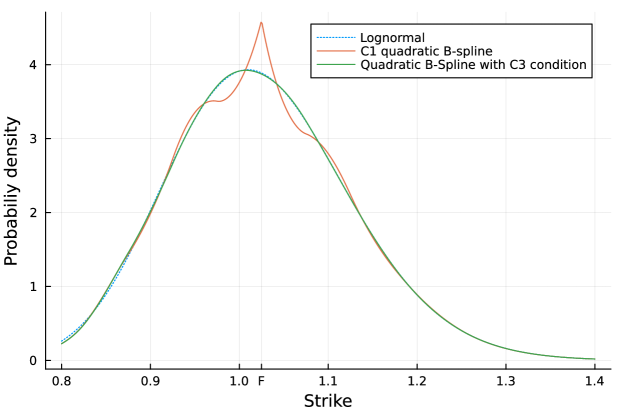
Figure 1: Implied probability density for the quadratic LVG model with or without the $\mathcal{C}^{3}$ condition (Equation 6), fitted to a Black-Scholes model with constant volatility $\sigma_{B}=20\%$, time to expiry $T=0.25$ and forward $1.025$.

5 Calibration

5.1 Error measure

The calibration of a single maturity consists in finding the parameters (the $\bm{\alpha}$ for the linear models, or $\bm{\lambda}$ for the quadratic B-spline) such that the function $C(x,T)$, solution of the Dupire PDDE fits the market option prices $(\hat{C}_{i})_{i=1,...n}$ of respective strikes $(K_{i})_{i=1,...,n}$ according to an appropriate measure. A common practice is to perform a least-squares minimization of the error measure $E$ defined by

$$E=\sum_{i=1}^{m}\mu_{i}^{2}\left(\sigma(\alpha,x_{i})-\hat{\sigma}_{i}\right)^{2}\,,$$ (18)

with $\alpha_{i}>0$ for $i=1,...,m$ and where $\sigma(\alpha,x)$ is the implied volatility corresponding to the option prices obtained with the piecewise-linear local gamma variance model and $\hat{\sigma}_{i}$ is the market implied volatility at strike $x_{i}$, $(\mu_{i})_{i=1,...,m}$ are weights associated to the accuracy of the fit at each point.

In order to solve this non-linear least-squares problem, we will use the Levenberg-Marquardt algorithm as implemented by Klare and Miller (2013). The box constraints $\alpha_{i}>0$ can be added in a relatively straightforward manner to any Levenberg-Marquardt algorithm, through the projection technique described in (Kanzow et al., 2004), or through a variable transform from $\mathbb{R}$ to a subset of $\mathbb{R^{+}}$ (for example through the function $x\to x^{2}+\epsilon$ with some small positive $\epsilon$).

The implied volatility for a given option price may be found efficiently and accurately through the algorithm of Jäckel (2015). In general, we prefer to solve an almost equivalent formulation in terms of option prices, using the error measure $E_{V}$ defined by

$$E_{V}=\sum_{i=1}^{m}w_{i}^{2}\left(C(\alpha,x_{i})-\hat{C}_{i}\right)^{2}\,,$$ (19)

with $C(\alpha,x)$ being the local variance gamma option price with parameter $\alpha$ and strike $x$, and the capped inverse Vega weights $w_{i}$ given by

$$w_{i}=\min\left(\frac{1}{\nu_{i}},\frac{10^{6}}{X(0)}\right)\mu_{i}\,,$$ (20)

where $\nu_{i}=\frac{\partial\hat{C}_{i}}{\partial\sigma}$ is the Black-Scholes Vega corresponding the market option price $\hat{C}_{i}$, and $10^{6}$ is a cap applied to avoid numerical issues related to the limited machine accuracy (see Le Floc’h and Oosterlee (2019b); Le Floc’h (2021) for the justification).

5.2 Exact interpolation

Sometimes, it is desirable to interpolate a given set of reference prices nearly exactly. This is typically the case when the reference prices come from some prior model. We apply the same least-square minimization but choose the number of free parameters to be equal to the number of reference prices.

5.2.1 Linear models

For the linear models, this means to use $m=n$ and set $\alpha_{0}=\alpha_{1}$ and $\alpha_{m+1}=\alpha_{m}$ to model a flat extrapolation. In general, the market strikes will not include $X(0)$. In this case, $X(0)$ must be added to the knots $\{x_{i}\}_{i=1,...,m}$ used in the local variance gamma representation. This adds one more parameter $\alpha_{s}$ to the representation, where $s$ is the index corresponding to $X(0)$ in the set of knots. The value of $\alpha_{s}$ is not free, it is given by the $\mathcal{C}^{3}$ condition (Equation 6) and enforced through the iterative procedure described in the previous sections.

5.2.2 B-spline knots locations

For the linear Bachelier and Black parameterization, choosing the knots at the market strikes works well. The situation is more complex for the quadratic B-spline parameterization.

Let $(K_{i})_{i=1,...,n}$ be the market options strikes. Let the index $i_{F}$ be such that $K_{i_{F}}\leq F<K_{i_{F}+1}$. We may:

• place the knots at the market strikes (labeled "Strikes" in the figures)

  $$\bm{t}=\begin{cases}\left(L,L,L,K_{1},...,K_{i_{F}},F,F,K_{i_{F}+1},...,K_{n},U,U,U\right)&\textmd{ if }K_{i_{F}}\neq F\\ \left(L,L,L,K_{1},...,K_{i_{F}},F,K_{i_{F}+1},...,K_{n},U,U,U\right)&\textmd{ if }K_{i_{F}}=F\end{cases}\,,$$

  The dimension of $\bm{\lambda}$ is then $n_{\lambda}=n+5$ if $F\neq K_{i_{F}}$ and $n+4$ if $F=K_{i_{F}}$. The change in the number of dimensions suggests that the interpolation may change significantly when the forward price moves across a market strike.

• place the knots in the middle of market strikes. According to (De Boor, 1978, p. 61), the $\mathcal{C}^{1}$ quadratic spline is then solution to a diagonally dominant tridiagonal system, which increases the stability and reduce oscillations of the interpolation. There are however several ways to do it:

  • choose the direct mid-points (labeled "Mid-Strikes")

    $$\bm{t}=\begin{cases}\left(L,L,L,\frac{K_{1}+K_{2}}{2},...,\frac{K_{i_{F}-1}+K_{i_{F}}}{2},F,F,\frac{K_{i_{F}}+K_{i_{F}+1}}{2},...,\frac{K_{n-1}+K_{n}}{2},U,U,U\right)&\textmd{ if }F<\frac{K_{i_{F}}+K_{i_{F}+1}}{2}\\ \left(L,L,L,\frac{K_{1}+K_{2}}{2},...,\frac{K_{i_{F}-1}+K_{i_{F}}}{2},\frac{K_{i_{F}}+K_{i_{F}+1}}{2},F,F,...,\frac{K_{n-1}+K_{n}}{2},U,U,U\right)&\textmd{ if }F>\frac{K_{i_{F}}+K_{i_{F}+1}}{2}\\ \left(L,L,L,\frac{K_{1}+K_{2}}{2},...,\frac{K_{i_{F}-1}+K_{i_{F}}}{2},F,F,\frac{K_{i_{F}+1}+K_{i_{F}+2}}{2},...,\frac{K_{n-1}+K_{n}}{2},U,U,U\right)&\textmd{ if }F=\frac{K_{i_{F}}+K_{i_{F}+1}}{2}\end{cases}\,,$$

    The dimension of $\bm{\lambda}$ is then $n_{\lambda}=n+4$ if $F\neq K_{i_{F}}$ and $n+3$ if $F=K_{i_{F}}$.

  • choose the mid-points, excluding the point closest to the forward price $F$ (labeled "Mid-X")

    $$\bm{t}=\left(L,L,L,\frac{K_{1}+K_{2}}{2},...,\frac{K_{i_{F}-1}+K_{i_{F}}}{2},F,F,\frac{K_{i_{F}+1}+K_{i_{F}+2}}{2},...,\frac{K_{n-1}+K_{n}}{2},U,U,U\right)\,,$$

    The dimension of $\bm{\lambda}$ is then $n_{\lambda}=n+3$.

  • choose the mid-points, excluding the point closest to the forward price and placing the first and last strike in the middle of two knots (labeled "Mid-XX")

    $$\bm{t}=\left(L,L,L,\frac{3K_{1}-K_{2}}{2},\frac{K_{1}+K_{2}}{2},...,\frac{K_{i_{F}-1}+K_{i_{F}}}{2},F,F,\frac{K_{i_{F}+1}+K_{i_{F}+2}}{2},...,\frac{K_{n-1}+K_{n}}{2},\frac{3K_{n}-K_{n-1}}{2},U,U,U\right)\,,$$

    The dimension of $\bm{\lambda}$ is then $n_{\lambda}=n+5$.

• use a uniform discretization of $[K_{1},K_{n}]$ composed of $n+1$ points, and shift it such that the forward is exactly part of the knots and we have $n_{\lambda}=n+5$.

In each of those case, we make sure to add the forward price as a double knot, as well as the boundaries $L,U$. The dimension of $\bm{\lambda}$ implied by the knots is larger than the number of market strikes. We choose the extra parameters as such:

• if $n_{\lambda}=n+5$, we set $\lambda_{1}=\lambda_{2}=\lambda_{3}$, $\lambda_{n+3}=\lambda_{n+4}=\lambda_{n+5}$ and $\lambda_{i_{F}+3}$ is obtained from $\lambda_{i_{F}+2}$ and $\lambda_{i_{F}+4}$.

• if $n_{\lambda}=n+4$, we set $\lambda_{1}=\lambda_{2}=\lambda_{3}$, $\lambda_{n+3}=\lambda_{n+4}$ and $\lambda_{i_{F}+3}$ is obtained from $\lambda_{i_{F}+2}$ and $\lambda_{i_{F}+4}$.

• if $n_{\lambda}=n+3$, we set $\lambda_{1}=\lambda_{2}$, $\lambda_{n+2}=\lambda_{n+3}$ and $\lambda_{i_{F}+2}$ is obtained from $\lambda_{i_{F}+1}$ and $\lambda_{i_{F}+3}$.

In order to assess the various knots candidates, we consider the same example as in the previous section, but using a few different random sets of 10 strikes in the interval [85,140] and a forward price $F=101$ (Table 1).

Table 1: Sets of market strikes with a Black-Scholes volatility of 20% for a maturity $T=0.25$ and forward $F=101$.

Set	$K_{1}$	$K_{2}$	$K_{3}$	$K_{4}$	$K_{5}$	$K_{6}$	$K_{7}$	$K_{8}$	$K_{9}$	$K_{10}$
A	88.77	92.85	93.38	99.37	107.99	120.29	122.03	123.9	134.71	135.43
B	85.02	101.92	103.55	114.45	121.85	123.69	125.07	125.58	131.63	133.86
C	98.07	100.93	101.06	106.88	109.12	110.93	119.76	119.83	132.19	138.27
D	85.00	90.00	95.00	100.00	101.00	105.00	110.00	115.00	120.00	130.00

Table 2: Root mean square error in implied volatilities % for various choices of B-spline knots. The reference volatilities are flat 20%.

Set	Strikes	Mid-Strikes	Mid-X	Mid-XX	Uniform
A	9.4e-8	6.0e-3	5.2e-3	4.1e-8	4.8e-9
B	9.9e-9	2.8e-3	5.8e-1	2.9e-6	9.9e-3
C	1.0e-6	1.9e-3	1.0e-2	1.1e-8	1.4e-3
D	4.1e-4	8.1e-2	4.1e-2	2.6e-5	5.0e-7

The uniform discretization may result in strong oscillations due to overfitting in places where no market strike is quoted as in the set A (Figure 2(a)).

The "Mid-Strikes" choice leads to a strong oscillation around the forward in set B (Figure 2(b)). The "Mid-X" produces a somewhat awkward shape on the set B. When the forward is very close to some of the knots as in set C, the "Strikes", "Mid-Strikes" choices lead to a density with a sharp gradient near the forward, a feature not desirable (Figure 2(c)). When the forward is part of the market strikes, a small wiggle is visible at the forward for "Strikes" and "Mid-Strikes" (Figure 2(d)).

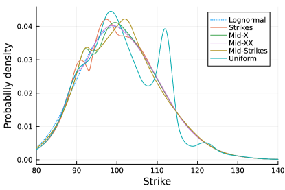
(a) Set A.

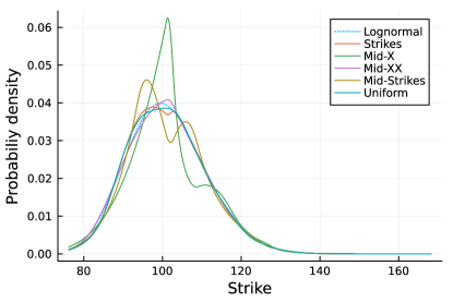
(b) Set B.

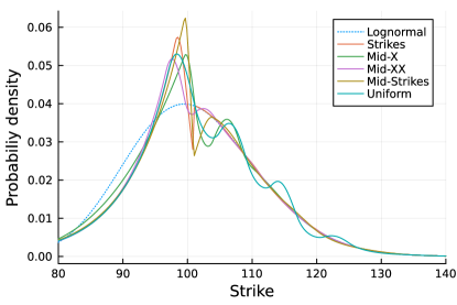
(c) Set C.

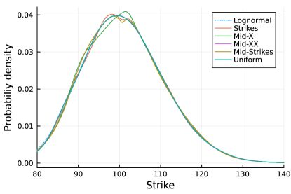
(d) Set D.

Figure 2: Implied probability density of the calibrated quadratic LVG model using different sets of knots.

Finally it is also interesting to look at the overall root mean square error in implied volatilities for the different choices (Table 2). The "Strikes" and "Mid-XX" choices consistently result in a near-perfect fit.

Overall, the "Mid-XX" knots lead to the most stable probability density along with an excellent fit.

5.2.3 Many quotes, few parameters

In (Le Floc’h, 2021), regularization is employed to ensure a smooth implied probability density when fitting to many, eventually noisy, market option quotes. An interesting simpler alternative is to use few knots/few parameters instead of as many parameters as market quotes: by limiting the number of free-parameters, we may avoid overfitting issues, and at the same time we reduce the number of dimensions of the problem, thus increasing stability and performance. Where to place the knots then? Based on the previous observations, we may choose knots such that the market strikes are equidistributed. Concretely, we use

$$\tilde{\bm{K}}=\left\{K_{1},K_{1+j},K_{1+2j},...,K_{n}\right\}\,,$$

where $j=n/m$ with $m\leq n$ and use the "Mid-XX" knots on top of $\tilde{\bm{K}}$. It may happen that many market strikes are quoted in a narrow range, in which case the set could be adjusted with a minimum strike width, although we did not need this tweak on the market examples presented below.

We consider several different underlying assets: SPX500 expiring on March 24, 2017 as March 16, 2017 (one week - 1w) and on March 7, 2018 as of February 5, 2018 (one month - 1m), TSLA of maturity July 20, 2018 as of June 15, 2018 (1m), AAPL with expiry in 4 days as of October 28, 2013 (4d) from Alexiou et al. (2021), as as well as the AUD/NZD currency pair of maturity July 9, 2014 as of July 2, 2014 (1w) from Wystup (2018). There is an apparent focus on short maturities as those are more difficult to capture, with a variety of smile shapes, with some exhibiting multi-modality. The latter are particularly challenging for parametric models such as SVI (Gatheral, 2006), SABR (Hagan et al., 2002), or even polynomial stochastic collocation (Le Floc’h and Oosterlee, 2019a, b). As the implied volatility smile flattens for long maturities, those are much easier to fit to.

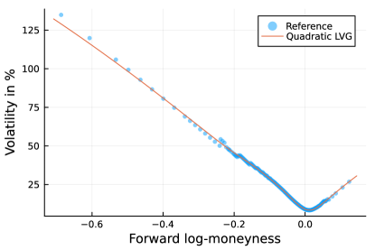
(a) Implied volatility.

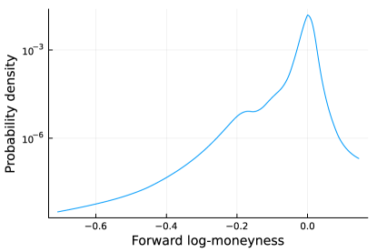
(b) Implied probability density in log scale.

Figure 3: Quadratic LVG model with 10 points calibrated to SPX500 options of maturity 1w.

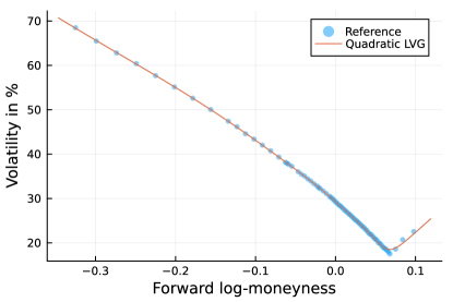
(a) Implied volatility.

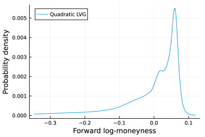
(b) Implied probability density.

Figure 4: Quadratic LVG model with 10 points calibrated to SPX500 options of maturity 1m.

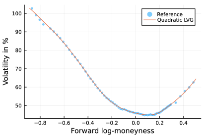
(a) Implied volatility.

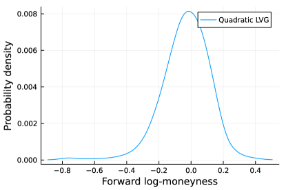
(b) Implied probability density.

Figure 5: Quadratic LVG model with 10 points calibrated to TSLA options of maturity 1m.

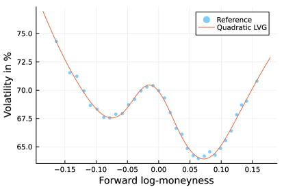
(a) Implied volatility.

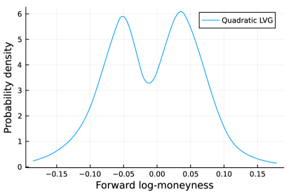
(b) Implied probability density.

Figure 6: Quadratic LVG model with 10 points calibrated to AAPL options of maturity 4d.

The AUD/NZD foreign exchange smile from Wystup (2018) is useful to see how the local variance gamma model behaves on a minimalistic example: indeed, as is usual on the foreign exchange options market, it involves only five options quotes. In this case we use as many parameters as market quotes. Figure 7(b) shows that the density implied by the quadratic LVG model is smooth, but the one implied by the linear Bachelier LVG model exhibits some sharp unnatural gradients near the money.

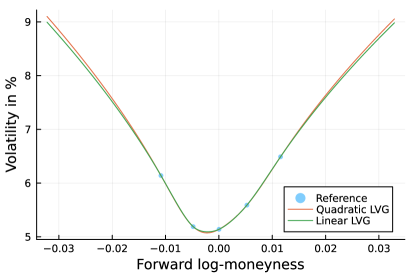
(a) Implied volatility.

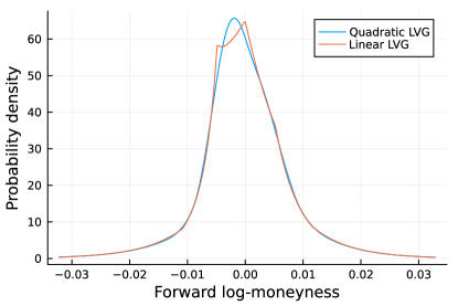
(b) Implied probability density.

Figure 7: Quadratic LVG model with 5 points calibrated to AUD/NZD options of maturity 1w.

Indeed, the linear LVG model leads only to a $\mathcal{C}^{0}$ probability density. Such gradients are then inevitable when the number of quotes is small. On this example, the (unconstrained) SVI model is known to lead to some negative probability density.

In all the examples considered so far, the fit in terms of implied volatilities is excellent, and the implied probability density is smooth, without spurious peaks, although the number of points considered ($n=10$) is somewhat arbitrary.

5.2.4 Challenging examples of exact interpolation

We consider the manufactured examples of Jäckel (2014) presented in Table 8. In the first example, a cubic spline interpolation of option prices is known to produce oscillations in the implied volatility, while a cubic spline on the volatilities introduces spurious arbitrages. In the second example, some of the quotes are at the limit of arbitrage.

On those examples, some care need to be taken in the choice of the boundaries $L$ and $U$: they must be far away enough. We pick $L=K_{1}/2$ and $U=2K_{m}$ where $K_{1}$ is the smallest quoted strike and $K_{m}$ the largest.

On the example case I, the fit is nearly exact for the linear Bachelier, Black and quadratic LVG models and there is no oscillation or wiggles in the implied volatility interpolation (Figure 8(a)). The corresponding implied probability density is of course smoothest with the quadratic LVG model (Figure 8(b)).

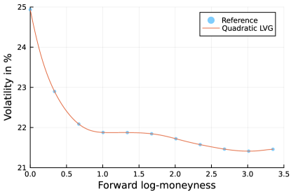
(a) Implied volatility.

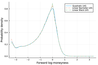
(b) Implied probability density in logarithmic scale.

Figure 8: LVG models calibrated to the example case I of Jäckel (2014).

On the example case II, the quadratic LVG model does not allow for an exact fit. The root mean square error is around 4 basis points (Table 3), the fit is qualitatively good (Figure 9(a)). The near-arbitrages impose the probability density to go to almost zero, which conflicts with the $\mathcal{C}^{1}$ continuity constraints of parameterized B-spline density. The density stays however smooth, and looks more natural than the clear overfit of the linear LVG models (Figure 9(b)).

(a) Implied volatility.

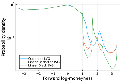
(b) Implied probability density in logarithmic scale.

Figure 9: LVG models calibrated to the example case II of Jäckel (2014).

Our choice of range for the $\bm{\alpha}$ parameter does not allow the linear Bachelier model to fit as well as the linear Black model. Increasing the range would make the two implied probability densities even more similar.

Table 3: Root mean square error (RMSE) in implied volatilities of the LVG models calibrated to the market data of Table 8.

Model	Case I	Case II
Linear Bachelier	5.00e-13	4.54e-6
Linear Black	3.64e-12	8.04e-8
Quadratic	2.25e-12	4.02e-4

6 Conclusion

The quadratic local variance gamma model with a small number of knots lead to smooth implied probability densities on a variety of market option quotes, while providing an excellent fit in terms of implied volatilities, even on challenging examples of non convex implied volatilities or multi-modal probability densities.

It thus constitutes an interesting alternative to the non-parametric approaches of the linear or quadratic local variance gamma models or of the Andreasen-Huge one-step local volatility model, which all require a non-trivial choice of regularization constant to produce a smooth implied probability density.

In similar fashion as Falck and Deryabin (2017), it may be used as specific generic parameterization with a fixed, small number of parameters using only 3 or 5 points. In contrast to Falck and Deryabin (2017), where the linear parameterization leads to edges in the implied probability density and where the problem of the discontinuity at the forward is not dealt with, the probability density of the quadratic LVG model with a reduced number of points will be smooth.

Further research may explore the use of Fourier transforms to recover efficient pricing formulae for European options under the local variance gamma model with a more general local variance function.

yes

no

Appendix A Avoiding the use of complex numbers

We have $\chi_{i}=\sqrt{\frac{a(x)}{\alpha_{i}}}$ and we know that $a(x)\geq 0$ since all the B-spline coefficients are positive, thus $\chi_{i}$ is either real or imaginary if the sign of $\alpha_{i}$ is positive (respectively strictly negative). Since $V(x)$ involves the ratio $\chi_{i}(x)/\chi_{i}(x_{i})$, we may equivalently calculate $\chi_{i}$ via $\chi_{i}=\sqrt{\frac{a(x)}{|\alpha_{i}|}}$.

From its definition, we know that $\omega_{i}$ is real if $\delta_{i}T+8\geq 0$ and imaginary otherwise.

For $z_{i}$ we need to consider the two cases where the roots $\tilde{x}_{i,1},\tilde{x}_{i,2}$ are both real or both complex.

If they are real, we have $\frac{x-\tilde{x}_{i,1}}{x-\tilde{x}_{i,2}}=\frac{a(x)}{\alpha_{i}(x-\tilde{x}_{i,2})^{2}}$. We know that $a(x)\geq 0$ since the B-spline coefficients are all positive. If $\alpha_{i}>0$ then $z_{i}$ is real, otherwise $z_{i}=\ln\left|\frac{x-\tilde{x}_{i,1}}{x-\tilde{x}_{i,2}}\right|+\mathrm{i}\mkern 1.0mu\pi$.

If the roots are complex with non null imaginary parts, $\tilde{x}_{i,1},\tilde{x}_{i,2}$ are conjugates of each other. We may write $\tilde{x}_{i,1}=u+\mathrm{i}\mkern 1.0muv$ and $\tilde{x}_{i,2}=u-\mathrm{i}\mkern 1.0muv$ with $(u,v)\in\mathbb{R}\times\mathbb{R}^{\star}$. We have then $\left|\frac{x-\tilde{x}_{i,1}}{x-\tilde{x}_{i,2}}\right|=\left|\frac{x-u-\mathrm{i}\mkern 1.0muv}{x-u+\mathrm{i}\mkern 1.0muv}\right|=1$ and thus $z_{i}$ is imaginary.

The term $\cosh\left(\omega_{i}\left(z_{i}(x)-z_{i}(x_{i})\right)\right)$ is thus always real. When $\omega_{i}\left(z_{i}(x)-z_{i}(x_{i})\right)$ is imaginary, the term $\sinh\left(\omega_{i}\left(z_{i}(x)-z_{i}(x_{i})\right)\right)$ is imaginary.

To evaluate the expression $V(x)$, there are four cases two consider:

• $\delta_{i}\geq 0$ and $\delta_{i}T+8\geq 0$. All the variables are real.

• $\delta_{i}\geq 0$ and $\delta_{i}T+8<0$. Take the absolute value in $\omega_{i}$, $\bar{\omega}_{i}=\frac{1}{2}\sqrt{\left|1+\frac{8}{\delta_{i}T}\right|}$. Then use $\sin$ instead of $\sinh$. $\Theta_{i}^{s}$ will then be real instead of complex.

• $\delta_{i}<0$ and $\delta_{i}T+8\geq 0$. The logarithm in $z_{i}$ may be calculated using $\Im\left(z_{i}(x)\right)=\arcsin\left[\Im\left(\frac{x-\tilde{x}_{i,1}}{x-\tilde{x}_{i,2}}\right)\right]$. The imaginary part may be directly calculated (without complex numbers). Then use $\cos\left[\bar{\omega}_{i}\Im\left(z_{i}(x)\right)\right]$, $\sin\left[-\bar{\omega}_{i}\Im\left(z_{i}(x)\right)\right]$ instead of $\cosh$ and $\sinh$ terms. $\Theta_{i}^{s}$ will then be real instead of complex.

• $\delta_{i}<0$ and $\delta_{i}T+8<0$. The logarithm in $z_{i}$ may be calculated using $\Im\left(z_{i}(x)\right)=\arcsin\left[\Im\left(\frac{x-\tilde{x}_{i,1}}{x-\tilde{x}_{i,2}}\right)\right]$. The imaginary part may be directly calculated (without complex numbers). Then use $\cosh\left[\bar{\omega}_{i}\Im\left(z_{i}(x)\right)\right]$, $\sinh\left[-\bar{\omega}_{i}\Im\left(z_{i}(x)\right)\right]$.

Appendix B Market data

Table 4: Implied volatilities SPX500 European options expiring on March 24, 2017 (one week, $T=0.021918$) assuming proportional dividends, with $r=0.9\%$ and implied forward $F(T)=2385.103981$. $y$ represents the log-moneyness $\ln\frac{K}{F}$ taken from Healy (2019).

Strike	$y$	Volume	Vol	Call Bid	Call Ask	Put Bid	Put Ask
1800	-0.2815	0	0.58	0.00	1.24	0.00	0.61
1850	-0.2541	3300	0.53	0.00	1.14	0.00	0.56
1875	-0.2406	3402	0.50	0.00	1.09	0.00	0.53
1880	-0.2380	1551	0.54	0.00	1.08	0.52	0.56
1890	-0.2327	200	0.53	0.00	1.06	0.51	0.55
1900	-0.2274	200	0.52	0.00	1.04	0.50	0.53
1910	-0.2221	0	0.49	0.00	1.02	0.00	0.52
1980	-0.1861	3	0.43	0.00	0.89	0.42	0.45
1990	-0.1811	2	0.43	0.00	0.87	0.41	0.45
2000	-0.1761	12	0.42	0.00	0.86	0.40	0.44
2010	-0.1711	1	0.41	0.00	0.84	0.39	0.43
2030	-0.1612	11	0.39	0.00	0.80	0.37	0.41
2035	-0.1587	1	0.38	0.00	0.79	0.36	0.40
2050	-0.1514	10	0.38	0.00	0.76	0.37	0.40
2055	-0.1490	10	0.38	0.00	0.75	0.36	0.39
2085	-0.1345	11	0.36	0.00	0.69	0.34	0.36
2090	-0.1321	1	0.35	0.00	0.69	0.34	0.36
2100	-0.1273	105	0.34	0.00	0.67	0.33	0.35
2105	-0.1249	1	0.33	0.00	0.66	0.32	0.34
2120	-0.1178	6	0.32	0.00	0.63	0.32	0.33
2125	-0.1155	111	0.32	0.00	0.62	0.31	0.33
2130	-0.1131	1	0.31	0.00	0.61	0.30	0.32
2135	-0.1108	11	0.31	0.00	0.61	0.30	0.31
2140	-0.1084	10	0.31	0.00	0.60	0.30	0.31
2150	-0.1038	6610	0.29	0.00	0.53	0.29	0.30
2155	-0.1015	1	0.29	0.00	0.52	0.28	0.30
2160	-0.0991	8	0.29	0.00	0.51	0.28	0.30
2165	-0.0968	2	0.28	0.00	0.50	0.28	0.29
2175	-0.0922	3	0.27	0.00	0.48	0.27	0.28
2180	-0.0899	66	0.27	0.00	0.47	0.27	0.28
2185	-0.0876	15	0.27	0.00	0.46	0.26	0.27
2190	-0.0853	26	0.26	0.00	0.45	0.26	0.27
2195	-0.0831	13	0.26	0.00	0.44	0.25	0.26
2200	-0.0808	113	0.25	0.00	0.43	0.25	0.25
2205	-0.0785	13	0.25	0.00	0.42	0.25	0.25
2210	-0.0762	14	0.24	0.00	0.41	0.24	0.25
2215	-0.0740	102	0.24	0.00	0.41	0.23	0.24
2220	-0.0717	2	0.23	0.00	0.40	0.23	0.24
2225	-0.0695	43	0.23	0.00	0.39	0.22	0.23
2230	-0.0672	93	0.22	0.00	0.38	0.22	0.23
2235	-0.0650	2	0.22	0.00	0.37	0.21	0.22
2240	-0.0628	134	0.21	0.00	0.36	0.21	0.22
2245	-0.0605	11	0.21	0.00	0.35	0.21	0.21
2250	-0.0583	104	0.20	0.00	0.34	0.20	0.21
2255	-0.0561	205	0.20	0.00	0.34	0.20	0.20
2260	-0.0539	184	0.19	0.00	0.33	0.19	0.20
2265	-0.0517	89	0.19	0.00	0.32	0.19	0.19
2270	-0.0495	74	0.18	0.00	0.28	0.18	0.19
2275	-0.0473	377	0.18	0.00	0.27	0.18	0.18
2280	-0.0451	207	0.17	0.00	0.26	0.17	0.17
2285	-0.0429	478	0.17	0.00	0.25	0.17	0.17
2290	-0.0407	295	0.16	0.00	0.24	0.16	0.17
2295	-0.0385	280	0.16	0.00	0.18	0.16	0.16
2300	-0.0363	1106	0.15	0.00	0.18	0.15	0.16
2305	-0.0342	377	0.15	0.00	0.17	0.15	0.15
2310	-0.0320	793	0.14	0.00	0.17	0.14	0.15
2315	-0.0298	567	0.14	0.09	0.16	0.14	0.14
2320	-0.0277	864	0.14	0.09	0.15	0.13	0.14
2325	-0.0255	569	0.13	0.10	0.15	0.13	0.13
2330	-0.0234	567	0.13	0.10	0.14	0.13	0.13
2335	-0.0212	260	0.12	0.10	0.14	0.12	0.12
2340	-0.0191	407	0.12	0.10	0.13	0.12	0.12
2345	-0.0170	506	0.12	0.10	0.13	0.11	0.12
2350	-0.0148	1850	0.11	0.10	0.12	0.11	0.11
2355	-0.0127	528	0.11	0.10	0.11	0.11	0.11
2360	-0.0106	1134	0.10	0.10	0.11	0.10	0.11
2365	-0.0085	436	0.10	0.10	0.10	0.10	0.10
2370	-0.0064	1063	0.10	0.09	0.10	0.10	0.10
2375	-0.0042	1420	0.09	0.09	0.10	0.09	0.10
2380	-0.0021	1248	0.09	0.09	0.09	0.09	0.09
2385	0.0000	229	0.09	0.09	0.09	0.09	0.09
2390	0.0021	2252	0.09	0.09	0.09	0.09	0.09
2395	0.0041	912	0.09	0.09	0.09	0.08	0.09
2400	0.0062	2650	0.09	0.08	0.09	0.08	0.09
2405	0.0083	2523	0.08	0.08	0.09	0.08	0.09
2410	0.0104	789	0.08	0.08	0.09	0.08	0.10
2415	0.0125	863	0.08	0.08	0.08	0.07	0.10
2420	0.0145	905	0.08	0.08	0.09	0.00	0.13
2425	0.0166	1178	0.09	0.08	0.09	0.00	0.13
2430	0.0187	815	0.09	0.08	0.09	0.00	0.14
2435	0.0207	267	0.09	0.09	0.09	0.00	0.15
2440	0.0228	402	0.09	0.09	0.09	0.00	0.16
2445	0.0248	50	0.09	0.09	0.09	0.00	0.17
2450	0.0268	2027	0.09	0.09	0.10	0.00	0.17
2455	0.0289	59	0.10	0.10	0.10	0.00	0.18
2460	0.0309	159	0.10	0.10	0.10	0.00	0.19
2465	0.0330	26	0.10	0.10	0.11	0.00	0.20
2470	0.0350	53	0.10	0.10	0.11	0.00	0.21
2475	0.0370	229	0.11	0.10	0.11	0.00	0.22
2495	0.0450	1	0.12	0.11	0.13	0.00	0.25
2550	0.0669	800	0.15	0.00	0.16	0.00	0.37

Table 5: Implied volatility quotes for SPX500 options expiring on March 7, 2018, as of February, 5, 2018. In ACT/365, the option maturity is $T=0.082192$. The implied forward price is $F(0,T)=2629.80$. The interest rate is $r=0.97\%$.

Strike	Logmoneyness	Implied vol.		Strike	Logmoneyness	Implied vol.
1900	-0.325055	0.684883		2650	0.007651	0.280853
1950	-0.299079	0.6548		2655	0.009536	0.277035
2000	-0.273762	0.627972		2660	0.011417	0.273715
2050	-0.249069	0.604067		2665	0.013295	0.270891
2100	-0.224971	0.576923		2670	0.01517	0.267889
2150	-0.201441	0.551253		2675	0.017041	0.264533
2200	-0.178451	0.526025		2680	0.018908	0.262344
2250	-0.155979	0.500435		2685	0.020772	0.258598
2300	-0.134	0.474137		2690	0.022632	0.2555
2325	-0.123189	0.461716		2695	0.024489	0.25219
2350	-0.112493	0.445709		2700	0.026343	0.249534
2375	-0.101911	0.433661		2705	0.028193	0.246659
2400	-0.09144	0.42016		2710	0.03004	0.243553
2425	-0.081077	0.407463		2715	0.031883	0.240202
2450	-0.070821	0.393168		2720	0.033723	0.236588
2470	-0.062691	0.381405		2725	0.03556	0.234574
2475	-0.060668	0.3793		2730	0.037393	0.230407
2480	-0.05865	0.377109		2735	0.039223	0.227866
2490	-0.054626	0.372471		2740	0.041049	0.223049
2510	-0.046626	0.360294		2745	0.042872	0.219888
2520	-0.04265	0.354671		2750	0.044692	0.218498
2530	-0.03869	0.350533		2755	0.046509	0.214702
2540	-0.034745	0.34419		2760	0.048322	0.210506
2550	-0.030815	0.339273		2765	0.050132	0.208175
2560	-0.026902	0.333069		2770	0.051939	0.205508
2570	-0.023003	0.328206		2775	0.053742	0.199967
2575	-0.021059	0.324314		2780	0.055542	0.199007
2580	-0.019119	0.322041		2785	0.057339	0.195062
2590	-0.015251	0.3168		2790	0.059133	0.190547
2600	-0.011397	0.310914		2795	0.060923	0.188427
2610	-0.007559	0.305042		2800	0.062711	0.185893
2615	-0.005645	0.302416		2805	0.064495	0.182878
2620	-0.003734	0.299488		2810	0.066276	0.179292
2625	-0.001828	0.29609		2815	0.068053	0.175001
2630	7.5E-05	0.292378		2835	0.075133	0.185751
2635	0.001974	0.289516		2860	0.083913	0.207173
2640	0.00387	0.28584		2900	0.097802	0.225248
2645	0.005762	0.283342

Table 6: Implied volatilities of TSLA European options expiring on July 20, 2018 as of June 15, 2018 ($T=0.095890$) with implied forward $F(T)=357.755926$.

Strike	Mid Vol in %	Weight	Strike	Mid Vol in %	Weight
150.0	102.7152094560499	1.7320508075688772	335.0	47.11478482467228	7.365459931328131
155.0	99.05195749900227	1.0	340.0	46.78835216769108	7.0992957397195395
160.0	96.57262376591365	1.224744871391589	345.0	46.56217516966071	7.628892449104261
165.0	94.05597986379826	1.0	350.0	46.299652559206564	7.461009761866454
175.0	91.81603362313814	2.738612787525831	355.0	45.939930288424485	8.706319543871567
180.0	90.19382314978117	1.558387444947959	360.0	45.856510564386596	8.78635305459552
185.0	88.46745842549402	1.9999999999999998	365.0	45.79048747963794	7.000000000000021
190.0	86.5754243981787	1.2602520756252087	370.0	45.52139844132191	7.745966692414834
195.0	84.561554924342	1.3301243435223526	375.0	45.3447302139774	8.093207028119338
200.0	82.45634579529838	2.273030282830976	380.0	45.04013827012644	6.16441400296897
205.0	80.28174604214972	1.3944333775567928	385.0	44.800472164335794	4.974937185533098
210.0	78.053958851195	1.2089410496539776	390.0	44.91995553643971	4.650268809434567
215.0	76.36802684802436	1.9999999999999998	395.0	44.78840707248649	4.315669125408015
220.0	74.54192306685303	2.0976176963403033	400.0	45.00659311379786	4.636809247747854
225.0	72.60651215584285	3.500000000000001	405.0	45.17530880150887	4.732863826479693
230.0	70.58414693439228	3.286335345030995	410.0	44.99007489879635	3.1144823004794873
235.0	68.49143304434797	2.6692695630078282	415.0	44.8814967685824	2.8809720581775857
240.0	66.3409356115238	2.7838821814150116	420.0	45.16047756853698	2.8284271247461894
245.0	64.6230979973991	3.1622776601683804	425.0	45.63938928347205	2.7718093060793882
250.0	63.0129173926189	3.605551275463988	430.0	46.002220642176724	4.092676385936223
255.0	61.30540004186168	3.3541019662496834	435.0	46.102443173801966	2.7041634565979926
260.0	59.469230763484425	3.0	440.0	46.40646817026155	2.652259934210953
265.0	58.11921286363728	2.9742484506432634	445.0	47.09795491400157	3.710691413905333
270.0	56.87314890047378	3.6469165057620923	450.0	47.625950451280104	3.777926319123662
275.0	55.39815904720001	3.8729833462074152	455.0	48.10009989573377	3.929942040850535
280.0	54.226712926697765	4.183300132670376	460.0	48.559069655772966	3.921096785339529
285.0	53.38887990387771	3.7505555144093887	465.0	49.06446878461756	3.70809924354783
290.0	52.34154661207794	4.1918287860346295	470.0	49.60612773473766	3.517811819867573
295.0	51.68510552270313	3.7670248460125917	475.0	50.11170526132832	3.3354160160315844
300.0	50.72806473672073	4.795831523312714	480.0	50.59204240563133	3.1622776601683777
305.0	49.979731599616564	4.527692569068711	500.0	51.591022062492634	1.3483997249264843
310.0	48.96563997378466	3.482097069296032	520.0	55.056251469410256	1.8929694486000912
315.0	48.23975850368014	3.2333489534143167	540.0	57.838819666460616	1.914854215512676
320.0	47.93681836406913	3.687817782917155	560.0	59.92609035805611	1.699673171197595
325.0	48.00058538405501	6.3245553203367555	580.0	62.59792014943735	1.8708286933869707
330.0	47.57525564073338	6.837397165588683

Table 7: Quotes for options on AUD/NZD currency pair of maturity July 9th, 2014 as of July 2nd, 2014. $S=1.0784,F(0,T)=1.07845,B(0,T)=0.999712587139$, 10-$\Delta$ RR = 0.35%, 25-$\Delta$ RR = 0.40%, ATM vol = 5.14%, 25-$\Delta$ BF = 0.25%, 10-$\Delta$ BF = 1.175%.

Maturity	10$\Delta$-Put	25$\Delta$-Put	ATM	25$\Delta$-Call	10$\Delta$-Call
1w	6.14%	5.19%	5.14%	5.59%	6.49%

Table 8: Black-Scholes implied volatilities against moneyness $\frac{x}{X(0)}$ for an option of maturity $T=5.0722$, examples 1 and 2 of Jäckel (2014).

Moneyness	Volatility (Case I)	Volatility (Case II)
0.035123777453185	0.642412798191439	0.649712512502887
0.049095433048156	0.621682849924325	0.629372247414191
0.068624781300891	0.590577891369241	0.598339248024188
0.095922580089594	0.553137221952525	0.560748840467284
0.134078990076508	0.511398042127817	0.518685454812697
0.18741338653678	0.466699250819768	0.473512707134552
0.261963320525776	0.420225808661573	0.426434688827871
0.366167980681693	0.373296313420122	0.378806875802102
0.511823524787378	0.327557513727855	0.332366264644264
0.715418426368358	0.285106482185545	0.289407658380454
1	0.249328882881654	0.253751752243855
1.39778339939642	0.228967051575314	0.235378088110653
1.95379843162821	0.220857187809035	0.235343538571543
2.73098701349666	0.218762825294675	0.260395028879884
3.81732831143284	0.218742183617652	0.31735041252779
5.33579814376678	0.218432406892364	0.368205175099723
7.45829006788743	0.217198426268117	0.417582432865276
10.4250740447762	0.21573928902421	0.46323707706565
14.5719954372667	0.214619929462215	0.504386489988866
20.3684933182917	0.2141074555437	0.539752566560924
28.4707418310251	0.21457985392644	0.566370957381163

References

- Alexiou et al. (2021) Alexiou, Lykourgos, Amit Goyal, Alexandros Kostakis, and Leonidas Rompolis. 2021. Pricing event risk: Evidence from concave implied volatility curves. Swiss Finance Institute Research Paper (21-48).
- Andreasen and Huge (2011) Andreasen, Jesper and Brian Huge. 2011. Volatility interpolation. Risk 24(3), 76.
- Breeden and Litzenberger (1978) Breeden, Douglas T and Robert H Litzenberger. 1978. Prices of state-contingent claims implicit in option prices. Journal of business, 621–651.
- Carr and Lee (2008) Carr, Peter and Roger Lee. 2008. Robust replication of volatility derivatives. In Prmia award for best paper in derivatives, mfa 2008 annual meeting.
- Carr and Madan (2001) Carr, Peter and Dilip Madan. 2001. Towards a theory of volatility trading. Option Pricing, Interest Rates and Risk Management, Handbooks in Mathematical Finance, 458–476.
- Carr and Nadtochiy (2017) Carr, Peter and Sergey Nadtochiy. 2017. Local variance gamma and explicit calibration to option prices. Mathematical Finance 27(1), 151–193.
- De Boor (1978) De Boor, Carl. 1978. A practical guide to splines, Volume 27. Springer-Verlag New York.
- Dupire (1994) Dupire, Bruno. 1994. Pricing with a smile. Risk 7(1), 18–20.
- Falck and Deryabin (2017) Falck, Markus and Mikhail Vladimirovich Deryabin. 2017. Local variance gamma revisited. Available at SSRN 2659728.
- Gatheral (2006) Gatheral, Jim. 2006. The volatility surface: a practitioner’s guide, Volume 357. Wiley. com.
- Hagan et al. (2002) Hagan, Patrick S, Deep Kumar, Andrew S Lesniewski, and Diana E Woodward. 2002. Managing smile risk. Wilmott magazine.
- Healy (2019) Healy, Jherek. 2019. Applied Quantitative Finance for Equity Derivatives. Lulu.com.
- Jäckel (2014) Jäckel, Peter. 2014. Clamping down on arbitrage. Wilmott 2014(71), 54–69.
- Jäckel (2015) Jäckel, Peter. 2015. Let’s be rational.
- Kahalé (2004) Kahalé, Nabil. 2004. An arbitrage-free interpolation of volatilities. Risk 17(5), 102–106.
- Kanzow et al. (2004) Kanzow, Christian, Nobuo Yamashita, and Masao Fukushima. 2004. Levenberg-marquardt methods for constrained nonlinear equations with strong local convergence properties. J. Computational and Applied Mathematics 172, 375–397.
- Klare and Miller (2013) Klare, Kenneth and Guthrie Miller. 2013. Gn–a simple and effective nonlinear least-squares algorithm for the open source literature.
- Le Floc’h (2021) Le Floc’h, Fabien. 2021. An arbitrage-free interpolation of class for option prices. The Journal of Derivatives 28(4), 64–86.