Memory Asymmetry Creates Heteroclinic Orbits to Nash Equilibrium
in Learning in Zero-Sum Games

Abstract

Learning in games considers how multiple agents maximize their own rewards through repeated games. Memory, an ability that an agent changes his/her action depending on the history of actions in previous games, is often introduced into learning to explore more clever strategies and discuss the decision-making of real agents like humans. However, such games with memory are hard to analyze because they exhibit complex phenomena like chaotic dynamics or divergence from Nash equilibrium. In particular, how asymmetry in memory capacities between agents affects learning in games is still unclear. In response, this study formulates a gradient ascent algorithm in games with asymmetry memory capacities. To obtain theoretical insights into learning dynamics, we first consider a simple case of zero-sum games. We observe complex behavior, where learning dynamics draw a heteroclinic connection from unstable fixed points to stable ones. Despite this complexity, we analyze learning dynamics and prove local convergence to these stable fixed points, i.e., the Nash equilibria. We identify the mechanism driving this convergence: an agent with a longer memory learns to exploit the other, which in turn endows the other’s utility function with strict concavity. We further numerically observe such convergence in various initial strategies, action numbers, and memory lengths. This study reveals a novel phenomenon due to memory asymmetry, providing fundamental strides in learning in games and new insights into computing equilibria.

Introduction

Learning in games discusses how players learn their strategies through repeated games (Fudenberg and Levine 1998). Here, whether or not players learn their optimal strategies, called Nash equilibrium, is a nontrivial problem because each player’s optimal strategy depends on the strategy of his/her opponent. This problem becomes further exacerbated in zero-sum games, where both the players conflict in their utility functions. In order to approach this problem, various learning algorithms have been proposed, such as replicator dynamics (Börgers and Sarin 1997; Hofbauer, Sigmund et al. 1998; Sato, Akiyama, and Farmer 2002) and gradient ascent (Singh, Kearns, and Mansour 2000; Zinkevich 2003; Bowling and Veloso 2002; Bowling 2004). The dynamics of these algorithms have undergone extensive study, with findings indicating a cycling behavior around the Nash equilibrium in zero-sum games (Mertikopoulos and Sandholm 2016; Mertikopoulos, Papadimitriou, and Piliouras 2018).

Memory, referring to an agent’s ability to alter their subsequent actions based on past decisions, is often incorporated into games to investigate more sophisticated strategies and explore the decision-making processes of real agents, such as humans. Such memory introduces greater complexity and diversity into games. A celebrated study in economics has shown that players with memory can take various strategies in the Nash equilibria (Fudenberg and Maskin 2009). Indeed, in prisoner’s dilemma games, agents with memory can achieve cooperation (Axelrod and Hamilton 1981) and asymmetric degree of cooperation (Fujimoto and Kaneko 2019), even though those without memories cannot cooperate in the Nash equilibrium. Memory also complicates learning dynamics such as chaotic dynamics (Barfuss, Donges, and Kurths 2019) and divergence from the Nash equilibrium (Fujimoto, Ariu, and Abe 2023) in zero-sum games. In recent years, theoretical approaches to games with memories have garnered significant interest (Barfuss 2020; Usui and Ueda 2021; Meylahn, Janssen et al. 2022; Ueda 2023).

How learning changes depending on memory length is an interesting question in games with memory. Indeed, this question has often been discussed in prisoner’s dilemma games. It is reported that agents with longer memories can cooperate more cleverly (Hilbe et al. 2017; Murase and Baek 2020). Furthermore, the difference in payoffs emerges between agents with different memory lengths in various learning algorithms such as Q-learning (Sandholm and Crites 1996), coupled replicator dynamics (Fujimoto and Kaneko 2021), and evolutionary dynamics (Baek et al. 2016; Schmid et al. 2022). This suggests that an asymmetry in memory capacities could potentially lead to the exploitation of the opponent’s payoff in zero-sum games. Despite this, the impact of memory asymmetry in games has yet to be thoroughly investigated.

This study considers learning in zero-sum games between agents with memory asymmetry. First, we formulate games with asymmetry memory and a gradient ascent algorithm in the games. This algorithm corresponds to replicator dynamics, provided that the learning rate is sufficiently small, as outlined in Fujimoto, Ariu, and Abe (2023). In order to catch theoretical insights, we first focus on two-action zero-sum games between agents with memory lengths of one and zero (called one-memory and zero-memory). We analyze the Nash equilibrium in this with-memory game in comparison with the “original” Nash equilibrium in games without memory. Interestingly, we prove that this original Nash equilibrium can be divided into two distinct regions. The first region comprises unstable fixed points within the learning dynamics, while the second consists of stable fixed points. These stable points correspond to the Nash equilibrium in with-memory games. Thus, heteroclinic orbits (Strogatz 2018) are observed in with-memory games; Dynamics diverge from the unstable region and converge to the stable region within the original Nash equilibrium. This convergence is because the agent with a longer memory learns to concave the opponent’s utility function. Furthermore, we experimentally confirmed this convergence across various initial states, action numbers, and memory lengths.

To summarize, our study uncovers complex heteroclinic dynamics in learning in with-memory games. We also identify a novel phenomenon of convergence in learning in zero-sum games, which is achieved due to memory asymmetry. Given that replicator dynamics exhibit cyclical behavior without memory (see Panel A in Fig. 1) and diverging behavior with memory symmetry (see Panel B), our discovery is significant (see Panel C).

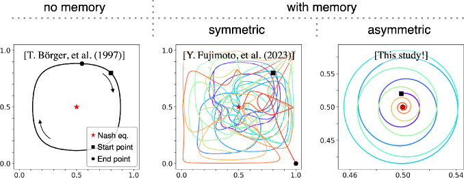
Figure 1: Learning dynamics illustrated for three memory-configuration scenarios involving two agents. Learning dynamics show a cycling behavior around the Nash equilibrium when the agents have no memory (left panel). Learning dynamics diverge from the Nash equilibrium when the agents have the same memory capacity (center). Learning dynamics draw heteroclinic orbits and eventually converge to the Nash equilibrium when the agents have different memory lengths (right). In all the panels, the horizontal and vertical axes indicate the probabilities of the agents choosing “head” in matching-pennies games (see Fig. 2). In the center and right panels, the color gradient indicates the passage of time (blue represents older data, and red represents newer data).

Preliminary

Two-Player Normal-Form Games

We consider two players of X and Y. In every round, each of them chooses its action from $\mathcal{A}=\{a_{1},\cdots,a_{m}\}$ and $\mathcal{B}=\{b_{1},\cdots,b_{m}\}$. If they choose $a\in\mathcal{A}$ and $b\in\mathcal{B}$, they immediately receive a payoff of $u_{ab}\in\mathbb{R}$ and $v_{ab}\in\mathbb{R}$, respectively. For the illustration of two-player normal-form games, see the area surrounded by the magenta dotted lines in Fig. 2-A.

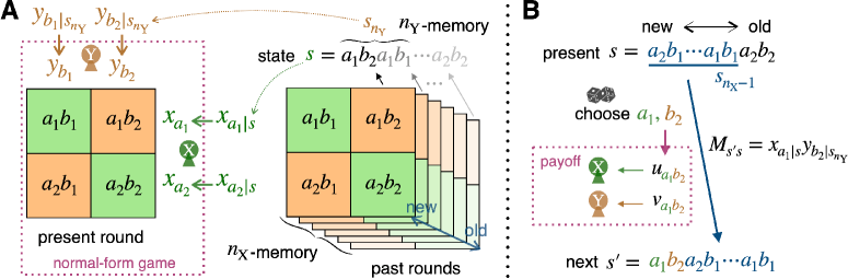
Figure 2: A: Schematics of with-memory games. The area surrounded by the magenta dotted line shows a classic normal-form game, where player X (green) chooses action either $a_{1}$ or $a_{2}$ with the probability of $x_{a_{1}}$ and $x_{a_{2}}$ in the row of the matrix, while player Y (orange) chooses action either $b_{1}$ or $b_{2}$ with the probability of $y_{b_{1}}$ and $y_{b_{2}}$ in the column. Especially in the matching-pennies game, $a_{1}=b_{1}=$ “head” and $a_{2}=b_{2}=$ “tail”. The matching of X’s and Y’s actions leads to X’s win (green panel), while the mismatching leads to Y’s win (orange panel). In with-memory games, $x_{a_{i}}$ and $y_{b_{i}}$ is given by $x_{a_{i}|s}$ and $y_{b_{i}|s_{n_{\rm Y}}}$. Here, $s$ is the string of their actions played in the previous $n_{\rm X}$ rounds. In addition, because Y has a shorter memory than X, $s_{n_{\rm Y}}$ is defined as the substring of $s$. B: Schematics of Markov transition in with-memory games. In the transition from $s$ to $s^{\prime}$, $s_{n_{\rm X}-1}$ (blue), i.e., the last $2(n_{\rm X}-1)$ substring of $s$ continues to exist in $s^{\prime}$. X and Y choose actions $a_{1}$ (green) and $b_{2}$ (orange) are appended to this substring $s_{n_{\rm X}-1}$. These choices occur with the probability of $M_{s^{\prime}s}$ and give X and Y the payoffs of $u_{a_{1}b_{2}}$ and $v_{a_{1}b_{2}}$, respectively.

Games with Memory Asymmetry

We assume that X and Y can memorize their actions in the newest $n_{\rm X}\in\mathbb{N}$ and $n_{\rm Y}\in\mathbb{N}$ rounds, respectively. We set that X has a longer memory ($n_{\rm X}>n_{\rm Y}$). Let $\mathcal{S}=\prod_{k=1}^{n_{\rm X}}(\mathcal{A}\times\mathcal{B})$ be the set of all states that X can memorize. Notably, each state $s\in\mathcal{S}$ is given by a string of actions of length $2n_{\rm X}$. Under state $s$, X can choose its action $a$ with the probability of $x_{a|s}\in(0,1)$. X’s strategy is the set of $x_{a|s}$ for all $a\in\mathcal{A}$ and $s\in\mathcal{S}$ and is denoted as $|\mathcal{S}|(=m^{2n_{\rm X}})$-numbers of $(m-1)$-dimension simplexes, ${\bf x}\in\prod_{s\in\mathcal{S}}\Delta^{m-1}$. Fig. 2-A shows the introduction of memories into normal-form games.

For each $n\in\{0,\ldots,n_{\rm X}-1\}$, let $s_{n}$ denote the newest $n$ substring of $s$. We also define the set $\mathcal{S}_{n}$ as $\mathcal{S}_{n}=\prod_{k=1}^{n}(\mathcal{A}\times\mathcal{B})$, which represents the set of all possible $s_{n}$. Since the length of Y’s memory is $n_{\rm Y}(<n_{\rm X})$, the set of states memorized by Y can be represented by $\mathcal{S}_{n_{\rm Y}}$. We assume that under each state $s_{n_{\rm Y}}$, Y chooses its action $b$ with probability $y_{b|s_{n_{\rm Y}}}\in(0,1)$. If $n_{\rm Y}=0$, $\mathcal{S}_{n_{\rm Y}}=\emptyset$ and we simply denote $y_{b|s_{n_{\rm Y}}}$ as $y_{b}$. Y’s strategy is given by ${\bf y}\in\prod_{s_{n_{\rm Y}}\in\mathcal{S}_{n_{\rm Y}}}\Delta^{m-1}$. Because the above immediate payoff is determined by both the players’ actions in the last round ($s_{1}\in\mathcal{A}\times\mathcal{B}$), we can rewrite the payoff as $u_{s_{1}}$ and $v_{s_{1}}$.

Formulation as Markov Transition Processes

The above setting is described by a discrete-time Markov transition process (see the illustration of Fig. 2-B), where the transition rate from state $s$ to $s^{\prime}$ is

$$M_{s^{\prime}s}({\bf x},{\bf y}):=\begin{cases}x_{a|s}y_{b|s_{n_{\rm Y}}}&(s^{\prime}=abs_{n_{\rm X}-1})\\ 0&({\rm otherwise})\\ \end{cases}.$$ (1)

We formulate the Nash equilibrium based on the Markov transition process. Then, strategies ${\bf x}$ and ${\bf y}$ may be regarded as fixed in the above Markov transition process. For fixed ${\bf x}$ and ${\bf y}$ within the interior of the simplexes, the stationary state for the above Markov transition processes is uniquely denoted as $p_{s}^{{\rm st}}({\bf x},{\bf y})$. The stationary state satisfies $p_{s^{\prime}}^{{\rm st}}({\bf x},{\bf y})=\sum_{s}M_{s^{\prime}s}({\bf x},{\bf y})p_{s}^{{\rm st}}({\bf x},{\bf y})$. If the game continues a sufficiently long time, each player’s payoff is given under this stationary state; $u^{{\rm st}}({\bf x},{\bf y})=\sum_{s}p_{s}^{{\rm st}}({\bf x},{\bf y})u_{s_{1}}$ and $v^{{\rm st}}({\bf x},{\bf y})=\sum_{s}p_{s}^{{\rm st}}({\bf x},{\bf y})v_{s_{1}}$. Therefore, the above payoffs reflect that every player learns slowly enough, i.e., their learning rates are sufficiently small. The Nash equilibrium is defined as the strategies that maximize their own payoff functions in the stationary state;

$$\begin{cases}{\bf x}^{*}\in\mathrm{argmax}_{{\bf x}}u^{{\rm st}}({\bf x},{\bf y}^{*})\\ {\bf y}^{*}\in\mathrm{argmax}_{{\bf y}}v^{{\rm st}}({\bf x}^{*},{\bf y})\\ \end{cases}.$$ (2)

The objective of this study is to learn this Nash equilibrium.

Algorithm

Referring to Fujimoto, Ariu, and Abe (2023), we now formulate the algorithm of multi-memory gradient ascent (MMGA) for asymmetric memory lengths between the players. This discretized algorithm can be implemented even when we do not know the analytical expression of $u^{{\rm st}}({\rm Norm}({\bf x}),{\bf y})$.

Algorithm 1 Discretized MMGA

Input: $\eta$, $\gamma$

1:  for $t=0,1,2,\cdots$ do

2:     for $a\in\mathcal{A}$, $s\in\mathcal{S}$ do

3:        ${\bf x}^{\prime}\leftarrow{\bf x}+\gamma{\bf e}_{a|s}$

4:        $\displaystyle\Delta_{a|s}\leftarrow\frac{u^{{\rm st}}({\rm Norm}({\bf x}^{\prime}),{\bf y})-u^{{\rm st}}({\bf x},{\bf y})}{\gamma}$

5:     end for

6:     for $a\in\mathcal{A}$, $s\in\mathcal{S}$ do

7:        $x_{a|s}\leftarrow x_{a|s}(1+\eta\Delta_{a|s})$

8:     end for

9:     ${\bf x}\leftarrow{\rm Norm}({\bf x})$

10:  end for

In Alg. 1, the initial states of ${\bf x}$ and ${\bf y}$ are set. In each time step of $t$, X shifts each component of ${\bf x}$ by $\gamma$ from the original strategy ${\bf x}$ and define ${\bf x}^{\prime}$ (line 3). Here, ${\bf e}_{a|s}$ is defined as the unit vector for the direction of $x_{a|s}$. Furthermore, we normalize ${\bf x}^{\prime}$ for each state as ${\rm Norm}({\bf x^{\prime}}):=\{x^{\prime}_{a|s}/(\sum_{a}x^{\prime}_{a|s})\}_{a,s}$. By comparing ${\rm Norm}({\bf x}^{\prime})$ with ${\bf x}$, X gets the gradient $\Delta_{a|s}$ (line 4). Using all of $\Delta_{a|s}$, X updates its strategy $x_{a|s}$ with learning rate $\eta$ (line 7) and normalizes it (line 8). Here, note that the update is weighted by $x_{a|s}$ itself. We also implement Alg. 1 for agent Y similarly. However, because Y has a shorter memory than X, its strategy is updated for $s_{n_{\rm Y}}\in\mathcal{S}_{n_{\rm Y}}$ instead of $s\in\mathcal{S}$. Y’s action $b\in\mathcal{B}$ and payoff $v^{{\rm st}}$ can be different from $a\in\mathcal{A}$ and $u^{{\rm st}}$.

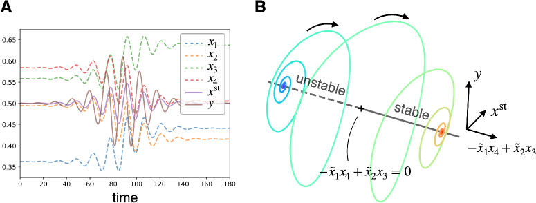
Figure 3: An example of heteroclinic orbit. A: Time series of $\boldsymbol{x}=(x_{1},x_{2},x_{3},x_{4})$, $x^{{\rm st}}(\boldsymbol{x},y)$, and $y$. B: Illustration of trajectories of learning dynamics. The trajectory is plotted in a three-dimensional space consisting of $x^{{\rm st}}(\boldsymbol{x},y)$, $y$, and $-\tilde{x}_{1}x_{4}+\tilde{x}_{2}x_{3}$. Only the solid line and the cross mark (i.e., $-\tilde{x}_{1}x_{4}+\tilde{x}_{2}x_{3}\geq 0$) is the Nash equilibrium, but the solid and dashed gray lines indicate the states that correspond to the original Nash equilibrium, i.e., $(x^{{\rm st}}(\boldsymbol{x},y),y)=(x^{\rm o},y^{\rm o})$. Note that this line should be a three-dimensional manifold in the five-dimensional space of $\boldsymbol{x}$ and $y$ in practice. The solid (resp. dashed) line satisfies the stable condition $-\tilde{x}_{1}x_{4}+\tilde{x}_{2}x_{3}>0$ (resp. $<0$). The trajectory is plotted from blue (time is $0$) to red (time is $180$) by the time series in panel A.

If the analytical expression of $u^{{\rm st}}({\bf x},{\bf y})$ and $v^{{\rm st}}({\bf x},{\bf y})$ are known, we can use the following dynamics (continualized MMGA (Fujimoto, Ariu, and Abe 2023)) instead of Alg. 1 by taking the limit of $\gamma\to 0$ and $\eta\to 0$;

$$\dot{x}_{a|s}({\bf x},{\bf y}) =x_{a|s}\frac{\partial}{\partial x_{a|s}}u^{{\rm st}}({\rm Norm}({\bf x}),{\bf y}),$$ (3)

$$\dot{y}_{b|s_{n_{\rm Y}}}({\bf x},{\bf y}) =y_{b|s_{n_{\rm Y}}}\frac{\partial}{\partial y_{b|s_{n_{\rm Y}}}}v^{{\rm st}}({\bf x},{\rm Norm}({\bf y})).$$ (4)

These continuous-time dynamics of the MMGA algorithm are useful for the theoretical treatment as they allow for classical stability analysis and numerical integration.

Theoretical Results

In this section, we analyze learning dynamics under asymmetric memory lengths between the players. To simplify theoretical treatments, we first establish several assumptions for the games, such as payoff matrix, action number, and memory length. Next, we derive the Nash equilibrium in these games and compare this equilibrium with the original Nash equilibrium in games without memory. Finally, we analyze the dynamics of learning. We prove that the fixed points of learning dynamics are divided into stable and unstable ones. Thus, heteroclinic dynamics diverging from unstable fixed points and converging to stable ones are drawn. In this section, we present only the proof sketch for each theorem, while detailed proofs can be found in Technical Appendix A.

Assumptions

First, we consider two-action zero-sum games as follows.

Assumption 1 (Two-action zero-sum game).

We denote the two actions of two agents as $\mathcal{A}=\{a_{1},a_{2}\}$ and $\mathcal{B}=\{b_{1},b_{2}\}$. There are four states $\mathcal{S}_{1}=\mathcal{A}\times\mathcal{B}=\{a_{1}b_{1},a_{1}b_{2},a_{2}b_{1},a_{2}b_{2}\}$. If each state occurs, X receives the payoff corresponding to $\boldsymbol{u}=(u_{1},\ldots,u_{4}):=(u_{a_{1}b_{1}},u_{a_{1}b_{2}},u_{a_{2}b_{1}},u_{a_{2}b_{2}})$. Zero-sum games assume that Y’s payoff is given by $v_{ab}=-u_{ab}$ for all $a\in\mathcal{A}$ and $b\in\mathcal{B}$. To ensure a nontrivial game, we assume that $u_{1}$ and $u_{4}$ are both larger than $u_{2}$ and $u_{3}$.

In Asm. 1, we consider a specific class of zero-sum games where the Nash equilibrium exists in the interior of the strategy spaces of two players. This is because if the Nash equilibrium is on the boundary of the strategy spaces, a dominant strategy exists and learning dynamics are trivial. An example that satisfies Asm. 1 is matching-pennies games ($u_{1}=u_{4}=+1$ and $u_{2}=u_{3}=-1$). Indeed, the Nash equilibrium is defined as follows.

Definition 1 (Original Nash equilibrium in two-action zero-sum normal-form game).

Under Asm. 1 (two-action zero-sum game), we consider $(n_{\rm X},n_{\rm Y})=(0,0)$ (no memory = normal-form game). Then, the mixed strategy of X is given by a single variable $x:=x_{a_{1}}\in(0,1)$. Similarly, Y’s strategy is given by $y:=y_{b_{1}}\in(0,1)$. Then, the Nash equilibrium $(x^{\rm o},y^{\rm o})$ and the payoffs in the equilibrium $(u^{\rm o},v^{\rm o})$ are given by

$$x^{\rm o}=\frac{-u_{3}+u_{4}}{u_{1}-u_{2}-u_{3}+u_{4}},\ y^{\rm o}=\frac{-u_{2}+u_{4}}{u_{1}-u_{2}-u_{3}+u_{4}},$$ (5)

$$u^{\rm o}=\frac{u_{1}u_{4}-u_{2}u_{3}}{u_{1}-u_{2}-u_{3}+u_{4}},\ v^{\rm o}=-u^{\rm o}.$$ (6)

The Nash equilibrium in no-memory games has been known for a long time (Nash Jr 1950). On the other hand, when agents with memories are considered, the region of the Nash equilibrium is generally extended (Fudenberg and Maskin 2009). Therefore, we call such a no-memory Nash equilibrium $(x^{\rm o},y^{\rm o})$ as the “original” Nash equilibrium for distinction.

We now introduce a specific class of with-memory games under Asm. 1 and define notations.

Definition 2 (One-memory and zero-memory strategies and vector notation).

Under Asm. 1, consider $(n_{\rm X},n_{\rm Y})=(1,0)$. Because a constraint $x_{a_{1}|s}+x_{a_{2}|s}=1$ holds for all $s\in\mathcal{S}=\{a_{1}b_{1},a_{1}b_{2},a_{2}b_{1},a_{2}b_{2}\}$, X’s strategy is determined by a four-variable vector $\boldsymbol{x}=(x_{1},\ldots,x_{4}):=(x_{a_{1}|a_{1}b_{1}},x_{a_{1}|a_{1}b_{2}},x_{a_{1}|a_{2}b_{1}},x_{a_{1}|a_{2}b_{2}})\in(0,1)^{4}$. On the other hand, Y’s strategy is determined by $y:=y_{b_{1}}\in(0,1)$. We also use the vector notation of the stationary state $\boldsymbol{p}^{{\rm st}}=(p_{1}^{{\rm st}},\ldots,p_{4}^{{\rm st}}):=(p_{a_{1}b_{1}}^{{\rm st}},p_{a_{1}b_{2}}^{{\rm st}},p_{a_{2}b_{1}}^{{\rm st}},p_{a_{2}b_{2}}^{{\rm st}})$. Expected payoffs in the stationary state are also described as $u^{{\rm st}}(\boldsymbol{x},y):=\boldsymbol{p}^{{\rm st}}(\boldsymbol{x},y)\cdot\boldsymbol{u}$ and $v^{{\rm st}}(\boldsymbol{x},y)=-u^{{\rm st}}(\boldsymbol{x},y)$.

Analysis of Nash Equilibrium

First, we provide an important theorem characterizing games between one-memory and zero-memory agents. In the following, we define $\tilde{\mathcal{X}}:=1-\mathcal{X}$ for any function or variable $\mathcal{X}$.

Theorem 1 (Stationary state).

Under Def. 2, the stationary state can be described as $\boldsymbol{p}^{{\rm st}}(\boldsymbol{x},y)=(x^{{\rm st}},\tilde{x}^{{\rm st}})\otimes(y,\tilde{y}):=(x^{{\rm st}}y,x^{{\rm st}}\tilde{y},\tilde{x}^{{\rm st}}y,\tilde{x}^{{\rm st}}\tilde{y})$. Here, $x^{{\rm st}}$ is called X’s “marginalized” strategy, a function of $(\boldsymbol{x},y)$;

$$x^{{\rm st}}(\boldsymbol{x},y)=\frac{x_{3}y+x_{4}\tilde{y}}{\tilde{x}_{1}y+\tilde{x}_{2}\tilde{y}+x_{3}y+x_{4}\tilde{y}}.$$ (7)

Proof Sketch. We consider the stationary state condition $p_{s^{\prime}}^{{\rm st}}=\sum_{s}M_{s^{\prime}s}p_{s}^{{\rm st}}$. Because Y uses zero-memory strategies, we derive $p_{1}^{{\rm st}}+p_{3}^{{\rm st}}=y$, $p_{2}^{{\rm st}}+p_{4}^{{\rm st}}=\tilde{y}$, and $p_{1}^{{\rm st}}/p_{2}^{{\rm st}}=p_{3}^{{\rm st}}/p_{4}^{{\rm st}}$. These three equations show that the stationary state is described as $\boldsymbol{p}^{{\rm st}}=(x^{{\rm st}},\tilde{x}^{{\rm st}})\otimes(y,\tilde{y})$ with a function $x^{{\rm st}}(\boldsymbol{x},y)$. By substituting this equation for the stationary state condition, we obtain the mathematical expression of $x^{{\rm st}}(\boldsymbol{x},y)$. ∎

Thm. 1 shows that in the stationary state, how each action is chosen by any one-memory strategy $\boldsymbol{x}\in(0,1)^{4}$ can be given by a zero-memory strategy $x=x^{{\rm st}}(\boldsymbol{x},y)$. Here, because $x^{{\rm st}}(\boldsymbol{x},y)$ is obtained by compressing $\boldsymbol{x}$ and $y$, we call it a “marginalized” strategy (following the terminology used in Press and Dyson (2012)). The representation of the marginalized strategy is as if X is using the no-memory strategy in the stationary state, but this is because opponent Y has no memory. However, note that this marginalized strategy $x^{{\rm st}}(\boldsymbol{x},y)$ is not a variable but a function that changes depending on the other’s strategy $y$. Based on Thm. 1, we obtain the Nash equilibrium as follows.

Theorem 2 (With-memory Nash equilibrium).

In with-memory games under Def. 2, $(\boldsymbol{x},y)=(\boldsymbol{x}^{*},y^{*})$ is the with-memory Nash equilibrium if and only if $x^{{\rm st}}(\boldsymbol{x}^{*},y^{*})=x^{\rm o}$, $y^{*}=y^{\rm o}$, and $-\tilde{x}_{1}^{*}x_{4}^{*}+\tilde{x}_{2}^{*}x_{3}^{*}\geq 0$ are satisfied.

Proof Sketch. We consider the extreme value conditions of X and Y. Using the notation of $\mathcal{F}|_{*}:=\mathcal{F}|_{(\boldsymbol{x},y)=(\boldsymbol{x}^{*},y^{*})}$ for any functions $\mathcal{F}$, we derive $\partial u^{{\rm st}}/\partial x_{i}|_{*}=0\Leftrightarrow y^{*}=y^{\rm o}$ for all $i$. Here, when $y=y^{\rm o}$, $u^{{\rm st}}$ is always constant independent of $\boldsymbol{x}$. We also derive $\partial v^{{\rm st}}/\partial y|_{*}=0\Leftrightarrow x^{{\rm st}}(\boldsymbol{x}^{*},y^{*})=x^{\rm o}$. Furthermore, the concavity condition of $v^{{\rm st}}$ for $y$ is given by

$$\frac{\partial^{2}v^{{\rm st}}(\boldsymbol{x}^{*},y)}{\partial y^{2}}\leq 0\ \ \Leftrightarrow\ \ \frac{\partial x^{{\rm st}}(\boldsymbol{x}^{*},y)}{\partial y}\geq 0$$

$$\Leftrightarrow\ \ -\tilde{x}_{1}^{*}x_{4}^{*}+\tilde{x}_{2}^{*}x_{3}^{*}\geq 0,$$ (8)

completing the proof. ∎

Let us discuss this with-memory Nash equilibrium, which is simply called Nash equilibrium below. First, $(\boldsymbol{x}^{*},y^{*})$ is a three-dimensional manifold in the space of $(\boldsymbol{x},y)$. In the space of $(x^{{\rm st}}(\boldsymbol{x},y),y)$, however, $(x^{{\rm st}}(\boldsymbol{x}^{*},y^{*}),y^{*})$ is unique and corresponds to the original Nash equilibrium $(x^{\rm o},y^{\rm o})$. Here, note that not all of $(\boldsymbol{x},y)$ such that $(x^{{\rm st}}(\boldsymbol{x},y),y)=(x^{\rm o},y^{\rm o})$ are the Nash equilibrium $(\boldsymbol{x}^{*},y^{*})$. This is because one more condition $-\tilde{x}_{1}^{*}x_{4}^{*}+\tilde{x}_{2}^{*}x_{3}^{*}\geq 0$ is necessary for the Nash equilibrium.

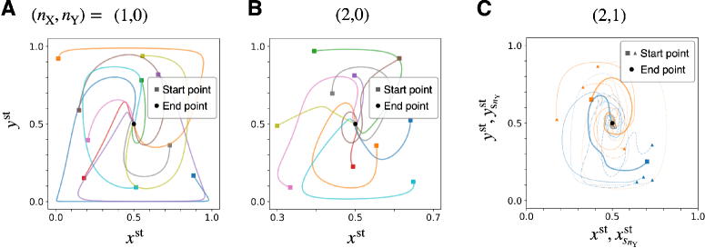
Figure 4: Learning dynamics for various asymmetric numbers of memories by removing Def. 2. Panels A and B show the cases of $(n_{\rm X},n_{\rm Y})=(1,0)$ and $(2,0)$, respectively. All the trajectories from various $10$ random initial states (represented by different colors) converge to the same Nash equilibrium. Panel C illustrates the case of $(n_{\rm X},n_{\rm Y})=(2,1)$. The horizontal and vertical axes indicate $x^{{\rm st}}$ and $y^{{\rm st}}$ for the wide thick lines, and X’s marginalized strategy $x_{s_{n_{\rm Y}}}^{{\rm st}}$ and Y’s strategy $y_{s_{n_{\rm Y}}}^{{\rm st}}$ for the other thin lines. The solid, dashed, dot, and dash-dot lines of the thin ones represent the cases of $s_{n_{\rm Y}}(=s_{1})=a_{1}b_{1}$, $a_{1}b_{2}$, $a_{2}b_{1}$, and $a_{2}b_{2}$, respectively. Both samples (represented by blue and orange) are observed to converge to the Nash equilibrium.

We also discuss this condition $-\tilde{x}_{1}^{*}x_{4}^{*}+\tilde{x}_{2}^{*}x_{3}^{*}\geq 0$. First, recall that X uses four variables $\boldsymbol{x}$ to construct a function $x^{{\rm st}}(\boldsymbol{x},y)$. As shown in Thm. 1, this function means the probability that X chooses action $a_{1}$ in the stationary state. Practically, however, X can change this probability depending on the other’s strategy $y$ because it has memory. $-\tilde{x}_{1}^{*}x_{4}^{*}+\tilde{x}_{2}^{*}x_{3}^{*}\geq 0$ is satisfied when $x_{1}^{*}$ and $x_{3}^{*}$ are large while $x_{2}^{*}$ and $x_{4}^{*}$ are small. In other words, X tends to use $a_{1}$ (resp. $a_{2}$) in response to $b_{1}$ (resp. $b_{2}$), meaning that X, in the next round, tries to use the advantageous action in response to the opponent’s action. Briefly said, X exploits Y’s payoff if Y biasedly chooses an action. Thus, it is best for Y to use its minimax strategy $y=y^{*}$. Indeed, $-\tilde{x}_{1}^{*}x_{4}^{*}+\tilde{x}_{2}^{*}x_{3}^{*}\geq 0$ is equivalent to $\partial^{2}v^{{\rm st}}(\boldsymbol{x}^{*},y)/\partial y^{2}\leq 0$, meaning that Y’s function is concave. Y cannot increase its own payoff even if it uses other strategies $y\neq y^{*}$. Thus, this condition is necessary for the Nash equilibrium.

Analysis of Learning Dynamics

Having discussed the appearance of a Nash equilibrium in a game with asymmetric memory, our attention will now be directed towards the dynamics of the game. Specifically, We now analyze the dynamics of Eqs. (3) and (4) around the equilibrium. Our first finding is that the fixed points of the learning dynamics correspond to the original Nash equilibrium.

Theorem 3 (Fixed points of learning dynamics).

Under Def. 2, all the fixed points of learning dynamics are given by $(x^{{\rm st}}(\boldsymbol{x},y),y)=(x^{\rm o},y^{\rm o})$.

Proof Sketch. Under Def. 2, Eqs. (3) and (4) are calculated as

$$\dot{x}_{i} =x_{i}\tilde{x}_{i}(u_{1}-u_{2}-u_{3}+u_{4})(y-y^{\rm o})\frac{\partial x^{{\rm st}}(\boldsymbol{x},y)}{\partial x_{i}},$$ (9)

$$\dot{y} =-y\tilde{y}(u_{1}-u_{2}-u_{3}+u_{4})$$

$$\hskip 8.5359pt\times\left\{(y-y^{\rm o})\frac{\partial x^{{\rm st}}(\boldsymbol{x},y)}{\partial y}+(x^{{\rm st}}(\boldsymbol{x},y)-x^{\rm o})\right\}.$$ (10)

We can calculate $(\dot{\boldsymbol{x}},\dot{y})=(\boldsymbol{0},0)\Leftrightarrow(x^{{\rm st}}(\boldsymbol{x},y),y)=(x^{\rm o},y^{\rm o})$. ∎

Next, the following theorem and corollary specify whether dynamics converge to or diverge from these fixed points.

Theorem 4 (Local convergence to Nash equilibrium).

Under Def. 2, the learning dynamics are locally asymptotically stable for each Nash equilibrium $(\boldsymbol{x}^{*},y^{*})$ such that $-\tilde{x}_{1}^{*}x_{4}^{*}+\tilde{x}_{2}^{*}x_{3}^{*}>0$.

Proof Sketch. We consider a linear stability analysis in the neighborhoods of the obtained fixed points. Let $\boldsymbol{J}$ denote the Jacobian matrix for learning dynamics with $\boldsymbol{z}=(\boldsymbol{x},y)$ and $J_{ij}:=\partial\dot{z}_{i}/\partial z_{j}|_{*}$. Each fixed point is locally stable when the maximum eigenvalue of the Jacobian except for $0$ (denoted as $\lambda_{1}$) is negative. We derive $\lambda_{1}<0\Leftrightarrow-\tilde{x}_{1}^{*}x_{4}^{*}+\tilde{x}_{2}^{*}x_{3}^{*}>0$, completing the proof. ∎

Corollary 1 (Divergence from fixed points).

Under Def. 2, if strategies $\boldsymbol{x}$ and $y$ satisfy $(x^{{\rm st}}(\boldsymbol{x},y),y)=(x^{\rm o},y^{\rm o})$, the strategies are fixed points of learning dynamics even in the region of $-\tilde{x}_{1}x_{4}+\tilde{x}_{2}x_{3}<0$. However, the strategies are unstable, and learning dynamics diverge from there.

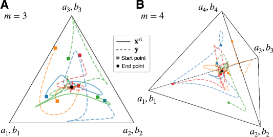
Figure 5: Learning dynamics for various numbers of actions are illustrated in two cases: (A) a rock-paper-scissors game ($m=3$), and (B) an extended rock-paper-scissors game with four actions ($m=4$). The dynamics of ${\bf x}^{{\rm st}}\in\Delta^{m-1}$ and ${\bf y}\in\Delta^{m-1}$ are plotted in each panel. The vertices of simplexes correspond to pure strategies for choosing actions $a_{1}$, $\cdots$, or $a_{m}$ in ${\bf x}^{{\rm st}}$ or $b_{1}$, $\cdots$, or $b_{m}$ in ${\bf y}$. In both cases, the samples of $4$ random initial conditions (indicated by different colors) converge to the Nash equilibrium.

Let us explain the property of learning dynamics from Thms. 3 and 4. First, Thm. 3 means that the fixed points of learning dynamics correspond to the original Nash equilibrium. However, learning dynamics do not converge to all of these fixed points. Thm. 4 shows that learning can converge to only roughly half of the fixed points where the condition $-\tilde{x}_{1}x_{4}+\tilde{x}_{2}x_{3}>0$ should be satisfied. Because the equivalence holds when all the inequalities become equalities in Eq. (8), this condition is equivalent to the strict concavity of Y’s utility function $v^{{\rm st}}(\boldsymbol{x},y)$.

Visualization of Heteroclinic Dynamics

Fig. 3 visualizes a heteroclinic orbit of learning dynamics. Panel A shows the time series of learning dynamics which is based on the continuous-time algorithm, i.e., the Runge-Kutta fourth-order method of Eqs. (3) and (4) with the step-size of $2\times 10^{-2}$. To facilitate interpretation, Panel B shows the trajectory of the time series of five-dimensional learning dynamics of $(\boldsymbol{x},y)$ in an appropriate three-dimensional space $(x^{{\rm st}},y,-\tilde{x}_{1}x_{4}+\tilde{x}_{2}x_{3})$. In panel B, all the gray solid and dashed lines correspond to the original Nash equilibrium, i.e., $(x^{{\rm st}},y)=(x^{\rm o},y^{\rm o})$ and to the fixed points of learning dynamics. In particular, the solid (resp. dashed) line shows stable (resp. unstable) fixed points of learning dynamics. Note that these one-dimensional lines represent a three-dimensional manifold in the five-dimensional space consisting of $(\boldsymbol{x},y)$. Now, we can see a heteroclinic orbit diverging from an unstable fixed point and converging to a stable one. Panel A illustrates an increase in $x_{1}$ and $x_{3}$, while $x_{2}$ and $x_{4}$ decrease through learning, indicating that X is learning to exploit Y. Consequently, $-\tilde{x}_{1}x_{4}+\tilde{x}_{2}x_{3}$ increases, leading to a concave utility function for Y with respect to $y$.

Experimental Results

So far, our theoretical analyses of learning dynamics have revealed the existence of heteroclinic orbits that converge to stable fixed points. In addition, these fixed points are included in the original Nash equilibrium of games without memory. In the following, we numerically confirm that learning dynamics converge to the original Nash equilibrium in various initial states, action numbers, and memory lengths. All the following experimental results are based on the discrete-time algorithm, i.e., Alg. 1. In the following, we set the inputs $\eta=10^{-3}$ and $\gamma=10^{-6}$ in Alg. 1. In computing gradients of payoff, i.e., $\Delta_{a|s}$, we calculate the equilibrium payoff accurately enough; The analytical solution $u^{{\rm st}}$ and computational solution $\hat{u}^{{\rm st}}$ satisfy $|u^{{\rm st}}-\hat{u}^{{\rm st}}|\leq 10^{-9}$.

Dynamics for Various Memory Lengths.

Fig. 4 shows that the learning dynamics converge to the Nash equilibrium in various numbers of memories. Panel A is for $(n_{\rm X},n_{\rm Y})=(1,0)$, B is for $(2,0)$, and C is for $(2,1)$. In Panel B, because $n_{\rm X}=2$, the number of variables that are necessary to describe X’s strategy $\boldsymbol{x}$ is larger than those in Def. 2. However, just like Thm. 1 shows, $\boldsymbol{x}$ construct the marginalized strategy of one function $x^{{\rm st}}(\boldsymbol{x},y)$ in the stationary state. Furthermore, the equilibrium corresponds to the original Nash equilibrium, i.e., $(x^{{\rm st}}(\boldsymbol{x},y),y)=(x^{\rm o},y^{\rm o})$. Notably, Panel C of $(n_{\rm X},n_{\rm Y})=(2,1)$ is interesting, where both the players memorize previous states as different from both A and B. X uses two-memory strategies given by sixteen variables $\boldsymbol{x}\in(0,1)^{16}$, while Y uses one-memory strategies given by four variables $\boldsymbol{y}\in(0,1)^{4}$. Then, $\boldsymbol{x}$ construct the marginalized strategy of four functions and X behaves as if X employs one-memory strategies. In conclusion, learning dynamics converge to the Nash equilibrium in games between one-memory strategies (Fujimoto, Ariu, and Abe 2023).

Dynamics for Various Action Numbers.

Next, we remove the assumption of two-action games (Asm. 1). Fig. 5 demonstrates that learning dynamics converge in various numbers of actions, where Panel A considers a Rock-Paper-Scissors game ($m=3$), while B considers an Extended Rock-Paper-Scissors game ($m=4$) with $(n_{\rm X},n_{\rm Y})=(1,0)$. From these panels, we can observe that learning dynamics converge in these games as in the two-action games. We now discuss where learning dynamics converge. Just like the proof in Thm. 1, we define the probability that X chooses action $a$ in the stationary state under $m$-action games as $x_{a}^{{\rm st}}({\bf x},{\bf y}):=\sum_{s\in\mathcal{S}}x_{a|s}p_{s}^{{\rm st}}({\bf x},{\bf y})$. We also define the set of $x_{a}^{{\rm st}}({\bf x},{\bf y})$ as ${\bf x}^{{\rm st}}({\bf x},{\bf y}):=\{x_{a}^{{\rm st}}({\bf x},{\bf y})\;|\;a\in\mathcal{A}\}$. Fig. 5 shows the last-iterate convergence to the Nash equilibrium, i.e., $({\bf x}^{{\rm st}}({\bf x},{\bf y}),{\bf y})=({\bf x}^{\rm o},{\bf y}^{\rm o})$. The mechanism for this convergence is similar to that in two-action games. Indeed, even in $m$-action zero-sum games, the player with $1$-memory endows a strict concavity to the utility function of the $0$-memory player (see the Technical Appendix C for a detailed explanation).

Experimental Results with Many Samples.

In order to ensure the reliability of our results, we have simulated the learning dynamics with a large number of samples with random initial strategies. In all the samples, we observed convergence to the Nash equilibrium. Refer to the Technical Appendix B for detailed data.

Discussion

This study explores the dynamics of learning in games where agents possess different memory capacities, both theoretically and experimentally. In our theoretical contributions, we assumed that two agents with memory lengths of one and zero play two-action zero-sum games. Under this assumption, we proved that the original Nash equilibrium in games without memory is divided into stable (Thm. 4) and unstable fixed points (Cor. 1) for learning. Here, heteroclinic orbits are discovered in learning in games with memory asymmetry; their strategies diverge from these unstable fixed points and converge to stable ones. In our experimental contributions, we relaxed the assumption on memory lengths and the number of actions, and then we demonstrated that memory asymmetry triggers this convergence to the original Nash equilibrium across a wider range of action numbers and memory lengths. Considering that dynamics show cycling behavior in games without memory and divergence in games with memory symmetry, this convergence is a nontrivial phenomenon.

Note that we have discovered new insights into computing equilibria, with memory asymmetry serving as one example. Convergent algorithms and dynamics, often referred to as last-iterate convergence, are extensively studied within the community of learning in games. The focus is mainly on computationally efficient algorithms with faster rates of convergence or global convergence guarantees (Daskalakis and Panageas 2019; Golowich, Pattathil, and Daskalakis 2020; Mertikopoulos et al. 2019; Wei et al. 2021; Lei et al. 2021; Nguyen et al. 2021; Anagnostides et al. 2022; Abe, Sakamoto, and Iwasaki 2022). In the majority of these studies, convergence is ensured through modifications to the learning algorithm. A typical example is to incorporate “optimism” symmetrically into discretized gradient ascent. Each agent then refines its strategy by naively predicting the opponent’s strategy update from past data (Daskalakis and Panageas 2019). Our method to achieve convergence differs significantly. We introduced memory asymmetry to alter the strategy spaces of one or both agents. By leveraging memory asymmetry, an agent with a longer memory learns to exploit the opponent’s payoff. Consequently, the opponent agent with a shorter memory achieves a strictly concave utility function, leading to convergence. To the best of our knowledge, this is the first study to induce convergence through such asymmetry of the strategy spaces. Our findings may open up new possibilities for achieving convergence in learning games and inspire further research in this field.

Technical Appendix

Appendix A Proofs

Proof of Theorem 1

Using the stationary state condition $p_{s^{\prime}}^{{\rm st}}=\sum_{s}M_{s^{\prime}s}p_{s}^{{\rm st}}$ is described for all $s^{\prime}$ as

$$p_{1}^{{\rm st}}=x_{1}yp_{1}^{{\rm st}}+x_{2}yp_{2}^{{\rm st}}+x_{3}yp_{3}^{{\rm st}}+x_{4}yp_{4}^{{\rm st}},$$ (A1)

$$p_{2}^{{\rm st}}=x_{1}\tilde{y}p_{1}^{{\rm st}}+x_{2}\tilde{y}p_{2}^{{\rm st}}+x_{3}\tilde{y}p_{3}^{{\rm st}}+x_{4}\tilde{y}p_{4}^{{\rm st}},$$ (A2)

$$p_{3}^{{\rm st}}=\tilde{x}_{1}yp_{1}^{{\rm st}}+\tilde{x}_{2}yp_{2}^{{\rm st}}+\tilde{x}_{3}yp_{3}^{{\rm st}}+\tilde{x}_{4}yp_{4}^{{\rm st}},$$ (A3)

$$p_{4}^{{\rm st}}=\tilde{x}_{1}\tilde{y}p_{1}^{{\rm st}}+\tilde{x}_{2}\tilde{y}p_{2}^{{\rm st}}+\tilde{x}_{3}\tilde{y}p_{3}^{{\rm st}}+\tilde{x}_{4}\tilde{y}p_{4}^{{\rm st}},$$ (A4)

By taking the summation of Eqs. (A1) and (A3) (resp. Eqs. (A2) and (A4)), we trivially obtain $p_{1}^{{\rm st}}+p_{3}^{{\rm st}}=y$ (resp. $p_{2}^{{\rm st}}+p_{4}^{{\rm st}}=\tilde{y}$). By using Eqs. (A1) and (A2) (resp. Eqs. (A3) and (A4)), we also obtain $p_{1}^{{\rm st}}/p_{2}^{{\rm st}}=y/\tilde{y}$ (resp. $p_{3}^{{\rm st}}/p_{4}^{{\rm st}}=y/\tilde{y}$). Thus, $p_{1}^{{\rm st}}/(p_{1}^{{\rm st}}+p_{3}^{{\rm st}})=p_{2}^{{\rm st}}/(p_{2}^{{\rm st}}+p_{4}^{{\rm st}})=:x^{{\rm st}}$ holds. From the definition of $x^{{\rm st}}$, the stationary state is described as $\boldsymbol{p}^{{\rm st}}=(x^{{\rm st}}y,x^{{\rm st}}\tilde{y},\tilde{x}^{{\rm st}}y,\tilde{x}^{{\rm st}}\tilde{y})=(x^{{\rm st}},\tilde{x}^{{\rm st}})\otimes(y,\tilde{y})$. Moreover, $x^{{\rm st}}$ is obtained as a function of $(\boldsymbol{x},y)$ by substituting $\boldsymbol{p}^{{\rm st}}=(x^{{\rm st}},\tilde{x}^{{\rm st}})\otimes(y,\tilde{y})$ into Eq. (A1);

$$x^{{\rm st}}y=x_{1}x^{{\rm st}}y+x_{2}x^{{\rm st}}\tilde{y}+x_{3}\tilde{x}^{{\rm st}}y+x_{4}\tilde{x}^{{\rm st}}\tilde{y}$$ (A5)

$$\Leftrightarrow x^{{\rm st}}(\boldsymbol{x},y)=\frac{x_{3}y+x_{4}\tilde{y}}{\tilde{x}_{1}y+\tilde{x}_{2}\tilde{y}+x_{3}y+x_{4}\tilde{y}}.$$ (A6)

∎

Proof of Theorem 2

First, we consider the extreme value condition for $u^{{\rm st}}$;

$$\left.\frac{\partial u^{{\rm st}}(\boldsymbol{x},y)}{\partial x_{i}}\right|_{*}=0 \Leftrightarrow\underbrace{\left.\frac{\partial x^{{\rm st}}(\boldsymbol{x},y)}{\partial x_{i}}\right|_{*}}_{\neq 0}\left\{(u_{1}-u_{2}-u_{3}+u_{4})y^{*}+(u_{2}-u_{4})\right\}=0,$$ (A7)

$$\Leftrightarrow y^{*}=\frac{-u_{2}+u_{4}}{u_{1}-u_{2}-u_{3}+u_{4}}=y^{\rm o}.$$ (A8)

When Eq. (A8) is satisfied, the payoff of X is always constant independent of $\boldsymbol{x}$ as

$$u^{{\rm st}}(\boldsymbol{x},y^{*}) =\boldsymbol{p}^{{\rm st}}(\boldsymbol{x},y^{*})\cdot\boldsymbol{u}$$ (A10)

$$=x^{{\rm st}}(\boldsymbol{x},y^{*})y^{*}u_{1}+x^{{\rm st}}(\boldsymbol{x},y^{*})\tilde{y}^{*}u_{2}+\tilde{x}^{{\rm st}}(\boldsymbol{x},y^{*})y^{*}u_{3}+\tilde{x}^{{\rm st}}(\boldsymbol{x},y^{*})\tilde{y}^{*}u_{4}$$ (A11)

$$=x^{{\rm st}}(\boldsymbol{x},y^{*})\underbrace{\left\{(u_{1}-u_{2}-u_{3}+u_{4})y^{*}+u_{2}-u_{4}\right\}}_{=0}+y^{*}(u_{3}-u_{4})+u_{4}$$ (A12)

$$=\frac{u_{1}u_{4}-u_{2}u_{3}}{u_{1}-u_{2}-u_{3}+u_{4}}$$ (A13)

$$=u^{\rm o}\ .$$ (A14)

Next, we consider the extreme value condition for $v^{{\rm st}}$;

$$\left.\frac{\partial v^{{\rm st}}(\boldsymbol{x},y)}{\partial y}\right|_{*}=0 \Leftrightarrow-\left.\frac{\partial x^{{\rm st}}(\boldsymbol{x},y)}{\partial y}\right|_{*}\underbrace{\left\{(u_{1}-u_{2}-u_{3}+u_{4})y^{*}+u_{2}-u_{4}\right\}}_{=0}$$

$$\hskip 12.80365pt-\left\{(u_{1}-u_{2}-u_{3}+u_{4})x^{{\rm st}}(\boldsymbol{x}^{*},y^{*})+u_{3}-u_{4}\right\}=0$$ (A15)

$$\Leftrightarrow x^{{\rm st}}(\boldsymbol{x}^{*},y^{*})=\frac{-u_{3}+u_{4}}{u_{1}-u_{2}-u_{3}+u_{4}}=x^{\rm o},$$ (A16)

In addition, using

$$\frac{\partial x^{{\rm st}}(\boldsymbol{x}^{*},y)}{\partial y} =\frac{-\tilde{x}_{1}^{*}x_{4}^{*}+\tilde{x}_{2}^{*}x_{3}^{*}}{(\tilde{x}_{1}^{*}y+\tilde{x}_{2}^{*}\tilde{y}+x_{3}^{*}y+x_{4}^{*}\tilde{y})^{2}},$$ (A17)

$$\frac{\partial^{2}x^{{\rm st}}(\boldsymbol{x}^{*},y)}{\partial y^{2}} =-2\frac{(-\tilde{x}_{1}^{*}x_{4}^{*}+\tilde{x}_{2}^{*}x_{3}^{*})(\tilde{x}_{1}^{*}-\tilde{x}_{2}^{*}+x_{3}^{*}-x_{4}^{*})}{(\tilde{x}_{1}^{*}y+\tilde{x}_{2}^{*}\tilde{y}+x_{3}^{*}y+x_{4}^{*}\tilde{y})^{3}}=-2\frac{\tilde{x}_{1}^{*}-\tilde{x}_{2}^{*}+x_{3}^{*}-x_{4}^{*}}{\tilde{x}_{1}^{*}y+\tilde{x}_{2}^{*}\tilde{y}+x_{3}^{*}y+x_{4}^{*}\tilde{y}}\frac{\partial x^{{\rm st}}(\boldsymbol{x}^{*},y)}{\partial y},$$ (A18)

we obtain

$$\frac{\partial^{2}v^{{\rm st}}(\boldsymbol{x}^{*},y)}{\partial y^{2}} =-\frac{\partial^{2}}{\partial y^{2}}(x^{{\rm st}}(\boldsymbol{x}^{*},y)yu_{1}+x^{{\rm st}}(\boldsymbol{x}^{*},y)\tilde{y}u_{2}+\tilde{x}^{{\rm st}}(\boldsymbol{x}^{*},y)yu_{3}+\tilde{x}^{{\rm st}}(\boldsymbol{x}^{*},y)\tilde{y}u_{4})$$ (A19)

$$=-(u_{1}-u_{2}-u_{3}+u_{4})2\frac{\partial x^{{\rm st}}(\boldsymbol{x}^{*},y)}{\partial y}-\left\{(u_{1}-u_{2}-u_{3}+u_{4})y+u_{2}-u_{4}\right\}\frac{\partial^{2}x^{{\rm st}}(\boldsymbol{x}^{*},y)}{\partial y^{2}}$$ (A20)

$$=-(u_{1}-u_{2}-u_{3}+u_{4})\left\{2\frac{\partial x^{{\rm st}}(\boldsymbol{x}^{*},y)}{\partial y}+(y-y^{*})\frac{\partial^{2}x^{{\rm st}}(\boldsymbol{x}^{*},y)}{\partial y^{2}}\right\}$$ (A21)

$$=-(u_{1}-u_{2}-u_{3}+u_{4})2\frac{\partial x^{{\rm st}}(\boldsymbol{x}^{*},y)}{\partial y}\left\{1-(y-y^{*})\frac{\tilde{x}_{1}^{*}-\tilde{x}_{2}^{*}+x_{3}^{*}-x_{4}^{*}}{\tilde{x}_{1}^{*}y+\tilde{x}_{2}^{*}\tilde{y}+x_{3}^{*}y+x_{4}^{*}\tilde{y}}\right\}$$ (A22)

$$=-(u_{1}-u_{2}-u_{3}+u_{4})2\frac{\partial x^{{\rm st}}(\boldsymbol{x}^{*},y)}{\partial y}\frac{\tilde{x}_{1}^{*}y^{*}+\tilde{x}_{2}^{*}\tilde{y}^{*}+x_{3}^{*}y^{*}+x_{4}^{*}\tilde{y}^{*}}{\tilde{x}_{1}^{*}y+\tilde{x}_{2}^{*}\tilde{y}+x_{3}^{*}y+x_{4}^{*}\tilde{y}}.$$ (A23)

Since $v^{{\rm st}}(\boldsymbol{x}^{*},y)$ should be concave for $y$, the condition

$$\frac{\partial^{2}v^{{\rm st}}(\boldsymbol{x}^{*},y)}{\partial y^{2}}\leq 0\ \ \Leftrightarrow\ \ \frac{\partial x^{{\rm st}}(\boldsymbol{x}^{*},y)}{\partial y}\geq 0\ \ \Leftrightarrow\ \ -\tilde{x}_{1}^{*}x_{4}^{*}+\tilde{x}_{2}^{*}x_{3}^{*}\geq 0,$$ (A24)

should be satisfied. ∎

Proof of Theorem 3

We can formulate continualized MMGA under Def. 2;

$$\dot{x}_{i} =x_{i}\tilde{x}_{i}\frac{\partial u^{{\rm st}}(\boldsymbol{x},y)}{\partial x_{i}}$$ (A25)

$$=x_{i}\tilde{x}_{i}\left\{(u_{1}-u_{2}-u_{3}+u_{4})y+(u_{2}-u_{4})\right\}\frac{\partial x^{{\rm st}}(\boldsymbol{x},y)}{\partial x_{i}}$$ (A26)

$$=x_{i}\tilde{x}_{i}(u_{1}-u_{2}-u_{3}+u_{4})(y-y^{\rm o})\frac{\partial x^{{\rm st}}(\boldsymbol{x},y)}{\partial x_{i}},$$ (A27)

$$\dot{y} =-y\tilde{y}\frac{\partial u^{{\rm st}}(\boldsymbol{x},y)}{\partial y}$$ (A28)

$$=-y\tilde{y}\left\{\frac{\partial x^{{\rm st}}(\boldsymbol{x},y)}{\partial y}\left\{(u_{1}-u_{2}-u_{3}+u_{4})y+(u_{2}-u_{4})\right\}+\left\{(u_{1}-u_{2}-u_{3}+u_{4})x^{{\rm st}}(\boldsymbol{x},y)+(u_{3}-u_{4})\right\}\right\}$$ (A29)

$$=-y\tilde{y}(u_{1}-u_{2}-u_{3}+u_{4})\left\{(y-y^{\rm o})\frac{\partial x^{{\rm st}}(\boldsymbol{x},y)}{\partial y}+(x^{{\rm st}}(\boldsymbol{x},y)-x^{\rm o})\right\}.$$ (A30)

Because $\partial x^{{\rm st}}(\boldsymbol{x},y)/\partial x_{i}\neq 0$, we obtain $\dot{\boldsymbol{x}}=\boldsymbol{0}\Leftrightarrow y=y^{\rm o}$. Further, when $y=y^{\rm o}$, we also obtain $\dot{y}=0\Leftrightarrow x^{{\rm st}}(\boldsymbol{x},y)=x^{\rm o}$. ∎

Proof of Theorem 4

We consider a neighborhood of the Nash equilibrium (i.e., $\boldsymbol{x}=\boldsymbol{x}^{*}+\mathrm{d}\boldsymbol{x}$ and $y=y^{*}+\mathrm{d}y$). Let $\boldsymbol{J}=(J_{ij})_{1\leq i\leq 5,1\leq j\leq 5}$ denote the Jacobian of learning dynamics;

$$J_{ij}:=\left\{\begin{array}[]{ll}\displaystyle\left.\frac{\partial\dot{x}_{i}}{\partial x_{j}}\right|_{*}=\left.x_{i}\tilde{x}_{i}\frac{\partial^{2}u^{{\rm st}}(\boldsymbol{x},y)}{\partial x_{i}\partial x_{j}}\right|_{*}&(1\leq i\leq 4,\ 1\leq j\leq 4)\\ \displaystyle\left.\frac{\partial\dot{x}_{i}}{\partial y}\right|_{*}=\left.x_{i}\tilde{x}_{i}\frac{\partial^{2}u^{{\rm st}}(\boldsymbol{x},y)}{\partial x_{i}\partial y}\right|_{*}&(1\leq i\leq 4,\ j=5)\\ \displaystyle\left.\frac{\partial\dot{y}}{\partial x_{j}}\right|_{*}=-\left.y\tilde{y}\frac{\partial^{2}u^{{\rm st}}(\boldsymbol{x},y)}{\partial y\partial x_{j}}\right|_{*}&(i=5,\ 1\leq j\leq 4)\\ \displaystyle\left.\frac{\partial\dot{y}}{\partial y}\right|_{*}=-\left.y\tilde{y}\frac{\partial^{2}u^{{\rm st}}(\boldsymbol{x},y)}{\partial y^{2}}\right|_{*}&(i=j=5)\\ \end{array}\right.\ .$$ (A35)

From the definitions of $\dot{\boldsymbol{x}}$ and $\dot{y}$, we obtain

$$\left.\frac{\partial\dot{x}_{i}}{\partial x_{j}}\right|_{*} =(u_{1}-u_{2}-u_{3}+u_{4})\left.\left\{(y-y^{\rm o})\frac{\partial}{\partial x_{j}}\left(x_{i}\tilde{x_{i}}\frac{\partial x^{{\rm st}}(\boldsymbol{x},y)}{\partial x_{i}}\right)\right\}\right|_{*}=0,$$ (A36)

$$\left.\frac{\partial\dot{x}_{i}}{\partial y}\right|_{*} =x_{i}^{*}\tilde{x}_{i}^{*}(u_{1}-u_{2}-u_{3}+u_{4})\left.\frac{\partial x^{{\rm st}}(\boldsymbol{x},y)}{\partial x_{i}}\right|_{*}>0,$$ (A37)

$$\left.\frac{\partial\dot{y}}{\partial x_{j}}\right|_{*} =-y^{*}\tilde{y}^{*}(u_{1}-u_{2}-u_{3}+u_{4})\left.\frac{\partial x^{{\rm st}}(\boldsymbol{x},y)}{\partial x_{j}}\right|_{*}<0,$$ (A38)

$$\left.\frac{\partial\dot{y}}{\partial y}\right|_{*} =-2y^{*}\tilde{y}^{*}(u_{1}-u_{2}-u_{3}+u_{4})\left.\frac{\partial x^{{\rm st}}(\boldsymbol{x},y)}{\partial y}\right|_{*}<0.$$ (A39)

We obtain the eigenvalues of matrix $\boldsymbol{J}$ as

$$\mathrm{det}(\lambda\boldsymbol{E}-\boldsymbol{J})=0$$ (A40)

$$\Leftrightarrow\lambda^{3}\left(\lambda^{2}-J_{55}\lambda-\sum_{i}J_{i5}J_{5i}\right)=0$$ (A41)

$$\Leftrightarrow\lambda=0\ ({\rm triple\ root}),\frac{J_{55}\pm\sqrt{J_{55}^{2}+4\sum_{i}J_{i5}J_{5i}}}{2}.$$ (A42)

Here, $J_{55}<0$ holds when $-\tilde{x}_{1}^{*}x_{4}^{*}+\tilde{x}_{2}^{*}x_{3}^{*}>0$, while $J_{i5}J_{5i}<0$ always hold. Thus, each of the interior points of the Nash equilibrium has two negative eigenvalues, and its basin of attraction [1] is two-dimensional in the five-dimensional space of $(\boldsymbol{x},y)$. Because the Nash equilibrium is spread over a three-dimensional space in $(\boldsymbol{x},y)$, the whole interior points of the Nash equilibrium are locally asymptotically stable (their basin of attraction is $3+2=5$-dimensional). ∎

Appendix B Experimental Results with More Samples

This section demonstrates that learning dynamics always converge to the Nash equilibrium, as shown in Fig. A1. We consider the five cases of $(m,n_{\rm X},n_{\rm Y})=(2,1,0)$ (blue panel), $(2,2,0)$ (orange), $(2,2,1)$ (green), $(3,1,0)$ (red), and $(4,1,0)$ (purple). We averaged $50$ samples of learning dynamics with random initial strategies for each case. As a measure for distance from equilibrium, we use the KL divergence to the marginalized strategies ${\bf z}^{{\rm st}}:=({\bf x}^{{\rm st}},{\bf y}^{{\rm st}})$ from the original Nash equilibrium ${\bf z}^{\rm o}:=({\bf x}^{\rm o},{\bf y}^{\rm o})$;

$$D_{\rm KL}({\bf z}^{\rm o}\|{\bf z}^{{\rm st}}):=\sum_{a\in\mathcal{A}}x_{a}^{\rm o}\log\frac{x_{a}^{\rm o}}{x_{a}^{{\rm st}}}+\sum_{b\in\mathcal{B}}y_{b}^{\rm o}\log\frac{y_{b}^{\rm o}}{y_{b}^{{\rm st}}}.$$ (A43)

Here, the marginalized strategy is defined by

$$x_{a}^{{\rm st}}:=\sum_{s\in\mathcal{S}}x_{a|s}p_{s}^{{\rm st}},\ \ \ y_{b}^{{\rm st}}:=\sum_{s\in\mathcal{S}}y_{b|s_{n_{\rm Y}}}p_{s}^{{\rm st}}.$$ (A44)

From Fig. A1, let us discuss learning dynamics in detail. The more the number of memories (blue $<$ orange $<$ green) is and the more the number of actions (blue $<$ red $<$ purple) is, the longer time the convergence takes. This is because the number of variables that construct each agent’s strategy increases with the number of memories and actions, and learning of the strategy gets slower with the increase in the number of such variables. Especially in the case of green panel $(m,n_{\rm X},n_{\rm Y})=(2,2,1)$, where both the agents have memories, complex dynamics are observed in a few samples; learning dynamics diverge from the Nash equilibrium once but converge there again.

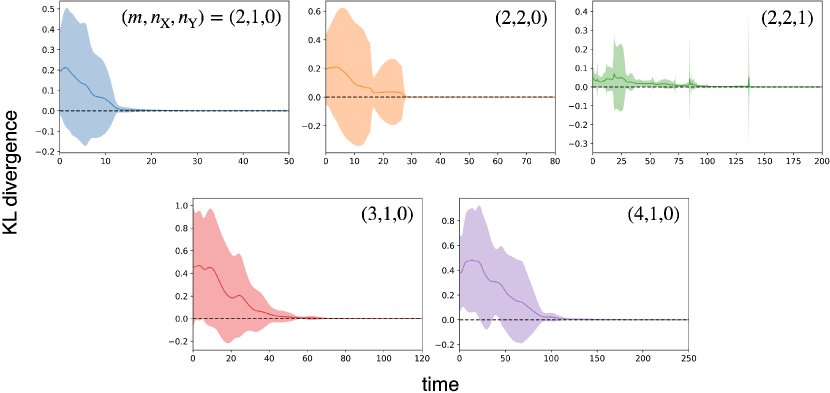
Figure A 1: Experimental results with many samples. In each panel, the solid line shows the mean value of KL divergence for $50$ samples. The lightly colored area shows the standard deviation estimated from the $50$ samples. When $m=2$, we consider a matching-pennies game, where $x_{a}^{\rm o}=y_{b}^{\rm o}=1/2$ for all $a$ and $b$. When $m=3$, we consider a rock-paper-scissors game, where $x_{a}^{\rm o}=y_{b}^{\rm o}=1/3$ for all $a$ and $b$. When $m=4$, we consider an extended-rock-paper-scissors game, where $x_{a}^{\rm o}=y_{b}^{\rm o}=1/4$ for all $a$ and $b$.

Appendix C Convergence Mechanism in $m$-Action Games

This section explains the convergence mechanism in $m$-action games between $1$-memory and $0$-memory players. In fact, Fig. A2 shows that the longer-memory X learns to endow the other Y’s utility function with a strict concavity in three-player zero-sum games, the ordinary (left panel) and biased (center) rock-paper-scissors games. Here, Y’s utility function takes its maximum value at the Nash equilibrium, leading to convergence. Thus, the convergence to the Nash equilibrium is induced by the strict concavity of Y’s utility function, as also seen in the case of two-action zero-sum games. If X has no memory, Y’s utility function is always linear (right) and Y fails to converge to the Nash equilibrium.

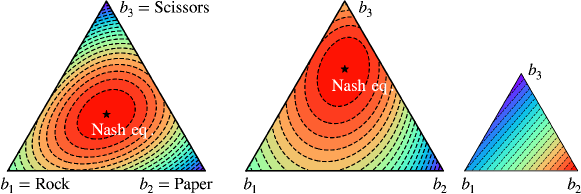
Figure A 2: Under X’s strategy fixed after it learns, Y’s utility function is plotted depending on Y’s strategy, i.e., ${\bf y}=\{y_{1},y_{2},y_{3}\}$. In all the panels, the red (blue) color indicates that Y’s utility is large (small). The lower-left point of the simplex indicates that Y purely takes $b_{1}=$Rock action (i.e., $y_{1}=1$). The lower-right point indicates $b_{2}=$Paper action (i.e., $y_{2}=1$). The upper-middle point indicates $b_{3}=$Scissors action (i.e., $y_{3}=1$). In the ordinary (left) and weighted (center) rock-paper-scissors games, Y’s utility function is strictly concave and takes its maximum value in the Nash equilibrium. In the right panel, X uses a $0$-memory strategy, and Y’s utility function is linear.

This strict concavity is given by a deadlock structure of actions, i.e., in rock-paper-scissors games, Rock $\to$ Paper $\to$ Scissors $\to$ Rock, and so on. Indeed, in Fig. A2, X tends to return Rock to the other’s Scissors, Paper to Rock, and Scissors to Paper. No matter how biasedly Y chooses its action, its payoff is exploited by such a strategy of X. Thus, Y maximizes its utility at its minimax strategy and is induced to the Nash equilibrium.

By extending the numerical result given by Fig. A2, we establish a conjecture that the similar strictly concave utility function may be seen in general zero-sum games with full-support equilibrium. Such games exhibit a cyclical structure of advantage among actions, akin to Rock $\to$ Paper $\to$ Scissors $\to$ Rock, and so on. The strict concavity is maintained when a $1$-memory player consistently chooses advantageous actions in response to the other’s previous choice of disadvantageous actions.

Appendix D Computational Environment

The simulations presented in this paper were conducted using the following computational environment.

• Operating System: macOS Monterey (version 12.4)

• Programming Language: Python 3.11.3

• Processor: Apple M1 Pro (10 cores)

• Memory: 32 GB

References

[1] Stephen Wiggins. Introduction to applied nonlinear dynamical systems and chaos, volume 2. Springer, 2003

References

• Abe, Sakamoto, and Iwasaki (2022) Abe, K.; Sakamoto, M.; and Iwasaki, A. 2022. Mutation-Driven Follow the Regularized Leader for Last-Iterate Convergence in Zero-Sum Games. In UAI, 1–10.
• Anagnostides et al. (2022) Anagnostides, I.; Panageas, I.; Farina, G.; and Sandholm, T. 2022. On last-iterate convergence beyond zero-sum games. In ICML, 536–581.
• Axelrod and Hamilton (1981) Axelrod, R.; and Hamilton, W. D. 1981. The evolution of cooperation. Science, 211(4489): 1390–1396.
• Baek et al. (2016) Baek, S. K.; Jeong, H.-C.; Hilbe, C.; and Nowak, M. A. 2016. Comparing reactive and memory-one strategies of direct reciprocity. Scientific reports, 6(1): 25676.
• Barfuss (2020) Barfuss, W. 2020. Reinforcement learning dynamics in the infinite memory limit. In AAMAS, 1768–1770.
• Barfuss, Donges, and Kurths (2019) Barfuss, W.; Donges, J. F.; and Kurths, J. 2019. Deterministic limit of temporal difference reinforcement learning for stochastic games. Physical Review E, 99(4): 043305.
• Börgers and Sarin (1997) Börgers, T.; and Sarin, R. 1997. Learning through reinforcement and replicator dynamics. Journal of Economic Theory, 77(1): 1–14.
• Bowling (2004) Bowling, M. 2004. Convergence and no-regret in multiagent learning. In NeurIPS, 209–216.
• Bowling and Veloso (2002) Bowling, M.; and Veloso, M. 2002. Multiagent learning using a variable learning rate. Artificial Intelligence, 136(2): 215–250.
• Daskalakis and Panageas (2019) Daskalakis, C.; and Panageas, I. 2019. Last-iterate convergence: Zero-sum games and constrained min-max optimization. In ITCS, 27:1–27:18.
• Fudenberg and Levine (1998) Fudenberg, D.; and Levine, D. K. 1998. The theory of learning in games, volume 2. MIT press.
• Fudenberg and Maskin (2009) Fudenberg, D.; and Maskin, E. 2009. The folk theorem in repeated games with discounting or with incomplete information. In A long-run collaboration on long-run games, 209–230. World Scientific.
• Fujimoto, Ariu, and Abe (2023) Fujimoto, Y.; Ariu, K.; and Abe, K. 2023. Learning in Multi-Memory Games Triggers Complex Dynamics Diverging from Nash Equilibrium. In IJCAI.
• Fujimoto and Kaneko (2019) Fujimoto, Y.; and Kaneko, K. 2019. Emergence of exploitation as symmetry breaking in iterated prisoner’s dilemma. Physical Review Research, 1(3): 033077.
• Fujimoto and Kaneko (2021) Fujimoto, Y.; and Kaneko, K. 2021. Exploitation by asymmetry of information reference in coevolutionary learning in prisoner’s dilemma game. Journal of Physics: Complexity, 2(4): 045007.
• Golowich, Pattathil, and Daskalakis (2020) Golowich, N.; Pattathil, S.; and Daskalakis, C. 2020. Tight last-iterate convergence rates for no-regret learning in multi-player games. In NeurIPS, 20766–20778.
• Hilbe et al. (2017) Hilbe, C.; Martinez-Vaquero, L. A.; Chatterjee, K.; and Nowak, M. A. 2017. Memory-n strategies of direct reciprocity. Proceedings of the National Academy of Sciences, 114(18): 4715–4720.
• Hofbauer, Sigmund et al. (1998) Hofbauer, J.; Sigmund, K.; et al. 1998. Evolutionary games and population dynamics. Cambridge university press.
• Lei et al. (2021) Lei, Q.; Nagarajan, S. G.; Panageas, I.; et al. 2021. Last iterate convergence in no-regret learning: constrained min-max optimization for convex-concave landscapes. In AISTATS, 1441–1449.
• Mertikopoulos et al. (2019) Mertikopoulos, P.; Lecouat, B.; Zenati, H.; Foo, C.-S.; Chandrasekhar, V.; and Piliouras, G. 2019. Optimistic mirror descent in saddle-point problems: Going the extra(-gradient) mile. In ICLR.
• Mertikopoulos, Papadimitriou, and Piliouras (2018) Mertikopoulos, P.; Papadimitriou, C.; and Piliouras, G. 2018. Cycles in adversarial regularized learning. In SODA, 2703–2717.
• Mertikopoulos and Sandholm (2016) Mertikopoulos, P.; and Sandholm, W. H. 2016. Learning in games via reinforcement and regularization. Mathematics of Operations Research, 41(4): 1297–1324.
• Meylahn, Janssen et al. (2022) Meylahn, J. M.; Janssen, L.; et al. 2022. Limiting dynamics for Q-learning with memory one in symmetric two-player, two-action games. Complexity, 2022.
• Murase and Baek (2020) Murase, Y.; and Baek, S. K. 2020. Five rules for friendly rivalry in direct reciprocity. Scientific reports, 10(1): 16904.
• Nash Jr (1950) Nash Jr, J. F. 1950. Equilibrium points in n-person games. Proceedings of the National Academy of Sciences, 36(1): 48–49.
• Nguyen et al. (2021) Nguyen, T.-D.; Zemhoho, A. B.; Tran-Thanh, L.; et al. 2021. Last round convergence and no-dynamic regret in asymmetric repeated games. In ALT, 553–577.
• Press and Dyson (2012) Press, W. H.; and Dyson, F. J. 2012. Iterated Prisoner’s Dilemma contains strategies that dominate any evolutionary opponent. Proceedings of the National Academy of Sciences, 109(26): 10409–10413.
• Sandholm and Crites (1996) Sandholm, T. W.; and Crites, R. H. 1996. Multiagent reinforcement learning in the iterated prisoner’s dilemma. Biosystems, 37(1-2): 147–166.
• Sato, Akiyama, and Farmer (2002) Sato, Y.; Akiyama, E.; and Farmer, J. D. 2002. Chaos in learning a simple two-person game. Proceedings of the National Academy of Sciences, 99(7): 4748–4751.
• Schmid et al. (2022) Schmid, L.; Hilbe, C.; Chatterjee, K.; and Nowak, M. A. 2022. Direct reciprocity between individuals that use different strategy spaces. PLoS Computational Biology, 18(6): e1010149.
• Singh, Kearns, and Mansour (2000) Singh, S.; Kearns, M. J.; and Mansour, Y. 2000. Nash Convergence of Gradient Dynamics in General-Sum Games. In UAI, 541–548.
• Strogatz (2018) Strogatz, S. H. 2018. Nonlinear dynamics and chaos with student solutions manual: With applications to physics, biology, chemistry, and engineering. CRC press.
• Ueda (2023) Ueda, M. 2023. Memory-two strategies forming symmetric mutual reinforcement learning equilibrium in repeated prisoners’ dilemma game. Applied Mathematics and Computation, 444: 127819.
• Usui and Ueda (2021) Usui, Y.; and Ueda, M. 2021. Symmetric equilibrium of multi-agent reinforcement learning in repeated prisoner’s dilemma. Applied Mathematics and Computation, 409: 126370.
• Wei et al. (2021) Wei, C.-Y.; Lee, C.-W.; Zhang, M.; and Luo, H. 2021. Linear Last-iterate Convergence in Constrained Saddle-point Optimization. In ICLR.
• Zinkevich (2003) Zinkevich, M. 2003. Online convex programming and generalized infinitesimal gradient ascent. In ICML, 928–936.