Abstract

During epidemics people reduce their social and economic activity to lower their risk of infection. Such social distancing strategies will depend on information about the course of the epidemic but also on when they expect the epidemic to end, for instance due to vaccination. Typically it is difficult to make optimal decisions, because the available information is incomplete and uncertain. Here, we show how optimal decision making depends on knowledge about vaccination timing in a differential game in which individual decision making gives rise to Nash equilibria, and the arrival of the vaccine is described by a probability distribution. We show that the earlier the vaccination is expected to happen and the more precisely the timing of the vaccination is known, the stronger is the incentive to socially distance. In particular, equilibrium social distancing only meaningfully deviates from the no-vaccination equilibrium course if the vaccine is expected to arrive before the epidemic would have run its course. We demonstrate how the probability distribution of the vaccination time acts as a generalised form of discounting, with the special case of an exponential vaccination time distribution directly corresponding to regular exponential discounting.

Introduction

Vaccination is the most successful tool against highly infectious diseases [1, 2]. In the absence of an effective vaccine, a wealth of alternative interventions become necessary. For instance, social distancing can be employed to reduce contacts with potentially infectious individuals at a social and economic cost to the individuals and to society at large [3]. There are many possible approaches to studying such behaviour [4]: The course of the epidemic and the behaviour of the population can be modelled in agent-based models [5, 6, 7] or compartmental mean field models, or on spatial [8] or temporal networks [9, 10]. The behaviour of the population can either be imposed ad-hoc or, increasingly commonly, it is assumed to arise from the decisions made by rational actors [11, 12, 13, 4, 14, 15], i.e. actors seeking to maximise an objective function with their actions. In centralised decision making, a central planner, typically a government, is assumed to be able to direct population behaviour directly to target the global optimum of the utility. In decentralised decision making, individuals optimise their own utility functional and as a population endogenously target a Nash equilibrium instead of a global utility maximum [11, 12, 13, 16, 15]. Finally, intervention schemes can be used by a social planner to incentivise individual behaviour such that the Nash equilibrium comes into alignment with the global optimum [17, 18, 19, 20].

What constitutes optimal or equilibrium behaviour is sensitive to the choice of objective function and to the parameters of the situation. Cost of infection, infectivity of the disease, effectiveness and cost of social distancing all play significant roles. In any case, social distancing is typically so costly that it cannot be carried out indefinitely. Since a population-scale vaccination event strongly impacts an epidemic, it is natural to ask how individuals should behave if they can expect such an event to occur. For the special case of when the future vaccination (or treatment) date is precisely known, equilibrium social distancing (of individuals) and optimal social distancing (enabled by a benevolent social planner) has been investigated already [11, 14]. In this situation social distancing behaviour will be the stronger the sooner the vaccination time is.

However, vaccination timing is usually not known precisely, especially not far in advance. It is more realistic to assume that the vaccination time is only known to follow a probability distribution. The simplest such assumption is one where for each unit time interval the vaccination is equally likely to arrive [15]. For such a situation the surprising result was reported that vaccination has no discernible effect on the decisions made by individuals. Here, we relax the assumption of uniformly likely arrival time and calculate equilibrium behaviour for any given vaccination arrival probability distribution. We calculate the optimal behaviour for all times on the condition that at any given time the vaccination has not arrived, yet. We show that in the formalism of expected utility theory, the vaccination time distribution can be interpreted as a form of generalised discounting, with an exponential distribution yielding the standard exponential discounting. We find that qualitatively the result that holds for sharp vaccination timing – that the earlier the vaccine can be expected to arrive, the stronger the social distancing will be – also holds for uncertain vaccination timing. In addition, we find that, for a series of probability distributions of increasing sharpness, the social distancing will be the stronger, the sharper the distribution is.

Not investigated by us is the case where the (costly) decision of whether or not to vaccinate (or receive other treatment) are under the control of individuals or a political decision maker, to be applied in an optimal manner over time [12, 4, 21] and/or space [22]. Here, vaccination is an exogenous event, being given to the whole population at once and for free. We assume that the vaccine works perfectly. The degree to which the vaccine protects from infection is important for rational decision making as well [23], but lies outside the scope of this work. We also neglect the loss of immunity in recovered people over time [18], for instance due to the emergence of new variants due to mutation [24] This and other complexities could be included in our approach in principle, such as multiple agent types with different risk and behaviour profiles [25, 13] or decentralised optimal behaviour via interventions orchestrated by a benevolent social planner.

In what follows, we first introduce the compartmental model for the disease, provide a definition for the Nash equilibrium in our system, then calculate the equilibrium behaviour for known vaccination time, and finally generalise this result to arbitrary vaccination probability distributions.

Methods

Epidemic dynamics

In our model, the epidemic follows a standard SIR compartmentalised model [26]. The population is composed of susceptible, infected and recovered compartments. The recovered compartment is meant to include the fraction of fatalities. The sizes of the compartments evolve over time as

$$\dot{s} =-k\>s\>i$$ (1)

$$\dot{i} =k\>s\>i-i$$ (2)

$$\dot{r} =i$$

with initial values $s(0)=1-i_{0}$ and $i(0)=i_{0}$ at a time $t=0$. Time derivatives are denoted with a dot. We measure time in units of the timescale of recovery from an infection. The control in this system is given by the population averaged infectiousness $k(t)$, which can be interpreted as the average number of new cases that would be caused by one infected individual in a fully susceptible population. We assume that the behaviour of the population determines $k(t)$, so we will directly call it behavior or control. In the absence of an epidemic, the population would exhibit a typical behaviour that corresponds to a default level of infectivity, $\kappa^{*}>1$. This value directly corresponds to the basic reproduction number $R_{0}$. Social distancing behaviour is expressed in the model as a reduction of $k$ away from $\kappa^{*}$. We drop the equation for the recovered compartment $r$ from here on, since its dynamics has no influence on the population behavior.

Nash equilibrium

In what follows, we assume that the population consist of identical individuals. The fate of any given individual can be described as a series of discrete transitions from one compartment to the next, at random times. Instead of modeling these jumps, we calculate the expected probabilities $\psi_{j}$ of said individual being in any of the compartments $j$. We assume that this individual can chose a behavior $\kappa(t)$ that is different from the average population behavior $k(t)$ and which influences the dynamics of these probabilities like

$$\dot{\psi}_{s} =-\kappa\psi_{s}i$$ (3)

$$\dot{\psi}_{i} =\kappa\psi_{s}i-\psi_{i}$$ (4)

with initial values $\psi_{s}(0)=s(0)$ and $\psi_{i}(0)=i(0)$. Being structurally quite similar to Eqs 2, these equations encode that the individual is infected by coming in contact with the population compartment $i$, which is obtained as the solution of those equations.

The individual is assumed to be choosing a behaviour that optimises a utility functional $U=U(\kappa(t),k(t))$. The notation exposes that the utility also depends on the population behaviour. If there is a Nash equilibrium in this system, it is given by a behavior $\kappa(t)$ that, if adopted by the population, the individual would have to select the same behaviour to optimise their utility

$$U(\hat{\kappa},\kappa)\leq U(\kappa,\kappa)\text{, for any }\kappa(t).$$ (5)

We can find the Nash equilibrium by, see [12] for details on the approach, by calculating the individual behaviour $\kappa(t)$ which maximises $U$ for a given, exogenous population behaviour $k(t)$. Then we self-consistently assume that all individuals would choose to optimise their behaviour in the same way and that therefore the expected population behavior is given by $\kappa=k$.

In what follows, we will first analyse the situation in which the vaccination time is precisely known to individuals at the outset, before deriving the generalisation for vaccination time distributions.

Individual decision making for known vaccination time

We analyse a simple stylised form for the individual (defector) utility with discounted utility per time $u$

$$U =\int_{0}^{\infty}u(t)dt$$ (6)

$$u =e^{-t/{\tau_{econ}}}\left[-\alpha\>\psi_{i}-\beta\>\psi_{s}(\kappa-\kappa^{*})^{2}\right]$$ (7)

Here, ${\tau_{econ}}$ is the economic discount time of an individual. The cost associated with infection $\alpha$ also includes the risk of death. The constant $\beta$ parameterises the financial and social costs associated with an individual modifying their behaviour from the baseline infectivity $\kappa^{*}$. We choose a quadratic form to ensure a natural equilibrium at $\kappa=\kappa^{*}$ in the absence of disease and/or intervention. We choose the units for the utility such that $\beta=1$ without loss of generality. This general form of the objective function is also used by [14], albeit in a somewhat different notation.

If vaccination occurs at $t_{v}$, immediately all remaining susceptibles are vaccinated and can be counted as recovered, i.e. $s(t>t_{v})=0$, and the remaining infectious recover exponentially. The utility cost of this recovery process after $t_{v}$ can be captured in a salvage term $U_{v}$. In other words, the salvage term represents the fact that it is regrettable for an individual – i.e. costly – to be infected at the moment the vaccination becomes available. We obtain, with the probability of being infected at vaccination time $\psi_{i}(t_{v})=\psi_{i,v}$ (for the derivation, see section A in the Supporting Information (SI))

$$U= \ \int_{0}^{t_{v}}u(t)dt+U_{v}$$ (8)

$$U_{v}= \ -\frac{e^{-t_{v}/{\tau_{econ}}}\alpha\,\psi_{i,v}}{{1/{\tau_{econ}}}+1}$$ (9)

Naturally, one can see that $U_{v}\to 0$ for $t_{v}\to\infty$.

Calculating the Nash equilibrium involves deriving differential equations for the adjoint values $v_{s}(t)$ and $v_{i}(t)$, which express the (economic) value of being in the given state at a given time, and an expression for the optimal control $k$, which are all being derived from the Hamiltonian of the system [27, 12]. The Hamiltonian for the individual behaviour during the epidemic consists of the individual cost function eq. 7 and of the equations describing the dynamics of the probabilities of an individual being in one of the relevant compartments, eq. 4,

$$H= -e^{-t/{\tau_{econ}}}\left[\alpha\psi_{i}+\beta\,\psi_{s}(\kappa-\kappa^{*})^{2}\right]$$ (10)

$$-(v_{s}-v_{i})\kappa\psi_{s}i-v_{i}\psi_{i}$$ (11)

Then, the equations for the expected present values of being in states $s$ and $i$ are

$$\dot{v}_{s} =-\frac{\partial H}{\partial\psi_{s}}=e^{-t/{\tau_{econ}}}\beta(\kappa-\kappa^{*})^{2}+(v_{s}-v_{i})\kappa i$$ (12)

$$\dot{v}_{i} =-\frac{\partial H}{\partial\psi_{i}}=e^{-t/{\tau_{econ}}}\alpha+v_{i}$$ (13)

The values are constrained by boundary conditions at the upper end of the integration interval of the utility derived from the vaccination salvage term, see SI, section A,

$$v_{s}(t_{v})=0,\ v_{i}(t_{v})=\ -\frac{e^{-t_{v}/{\tau_{econ}}}\alpha}{{1/{\tau_{econ}}}+1}$$ (14)

The optimal control for an individual follows from

$$0 =\frac{\partial H}{\partial\kappa}=-e^{-t/{\tau_{econ}}}\left[2\beta\psi_{s}(\kappa-\kappa^{*})\right]-(v_{s}-v_{i})i\psi_{s}$$ (15)

and reads

$$\kappa=\kappa^{*}-\frac{e^{t/{\tau_{econ}}}}{2\beta}(v_{s}-v_{i})i.$$ (16)

Assuming all individuals choose the same behaviour, we obtain the Nash behaviour, $k(t)=\kappa(t)$ and therefore $s=\psi_{s}$ and $i=\psi_{i}$,

$$k=\kappa=\kappa^{*}-\frac{e^{t/{\tau_{econ}}}}{2\beta}(v_{s}-v_{i})i.$$ (17)

Individual decision making under uncertainty

Until now we had assumed that a perfect vaccine becomes available at a set time $t_{v}$ and that the objective function $U$ yields the Nash equilibrium behaviour $\kappa(t)$; now, we explicitly acknowledge the role of $t_{v}$ in the notation and write this utility function as $U(\kappa,k,t_{v})$. However, the development schedule of vaccines is uncertain and it is more plausible to only assume knowledge of the probability distribution $p(t_{v})$ of the vaccination timing. Then, the expected individual utility under this uncertainty can be expressed as

$$\tilde{U}(\kappa,k)=\int_{0}^{\infty}p(t_{v})U(\kappa(t),k(t),t_{v})\,\mathrm{d}t_{v}.$$ (18)

with the Nash equilibrium behaviour defined by $\tilde{\kappa}(t)=\operatorname*{arg\,max}_{\kappa}(U(\kappa,k))$ and subsequently setting $k=\tilde{\kappa}$.

Naturally, the behaviour $\tilde{\kappa}(t)$ is only optimal for as long as the vaccine has not actually become available, yet. Immediately after the vaccination actually happens, the number of susceptibles drops to 0, and subsequently, the number of infections exponentially decays. In that case, social distancing becomes unnecessary.

To calculate the equilibrium, we found it necessary to first rewrite the utility. Inserting the general form of the utility as defined above, eq. 8, we have

$$\tilde{U}(\kappa,k)=\int_{0}^{\infty}p(t_{v})\left[\int_{0}^{t_{v}}u(\kappa(t),k(t))\,\mathrm{d}t+U_{v}(t_{v})\right]\,\mathrm{d}t_{v}$$ (19)

Note that $U_{v}(t_{v})$ in general depends on the state of the ODEs at $t_{v}$, i.e. $s(t_{v})$, $i(t_{v})$, $p_{s}(t_{v})$, $p_{i}(t_{v})$, etc., and therefore implicitly depends on the choice of $k$ and $\kappa$ as well. We drop this dependence from the notation for brevity. Starting to simplify,

$$\tilde{U}(\kappa,k) =\int_{0}^{\infty}p(t_{v})\int_{0}^{t_{v}}u(\kappa(t),k(t))\,\mathrm{d}t\,\mathrm{d}t_{v}$$ (20)

$$+\int_{0}^{\infty}p(t_{v})U_{v}(t_{v})\,\mathrm{d}t_{v}.$$ (21)

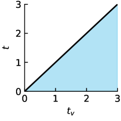
Fig S1: Sketch of the area over which we integrate in eq. 19. For each fixed $t_{v}$, we integrate $t$ from 0 to $t_{v}$. Alternatively, for fixed $t$, we can integrate $t_{v}$ from $t$ to $\infty$.

In order to apply the standard framework for expected utility optimisation, the integral over $t$ has to be the outer integral. By reversing the order of the integrals, see SI, fig. S1, we obtain

$$\tilde{U}(\kappa,k) =\int_{0}^{\infty}u(\kappa(t),k(t))\int_{t}^{\infty}p(t_{v})\,\mathrm{d}t_{v}\,\mathrm{d}t$$ (22)

$$+\int_{0}^{\infty}p(t_{v})U_{v}(t_{v})\,\mathrm{d}t_{v}.$$ (23)

With the cumulative distribution function

$$C(t)=\int_{0}^{t}p(t^{\prime})\,\mathrm{d}t^{\prime}$$ (24)

we can then write

$$\tilde{U}(\kappa,k) =\int_{0}^{\infty}u(\kappa(t),k(t))[1-C(t)]\,\mathrm{d}t$$ (25)

$$+\int_{0}^{\infty}p(t_{v})U_{v}(t_{v})\,\mathrm{d}t_{v}.$$ (26)

Renaming $t_{v}\to t$ in the second term, we obtain the averaged utility in a standard form

$$\tilde{U}(\kappa,k)=\int_{0}^{\infty}[1-C(t)]\,u(\kappa(t),k(t))+p(t)\,U_{v}(t)\,\mathrm{d}t.$$ (27)

which can be optimised equivalently to the approach for known vaccination time.

To facilitate numerical solution, we truncate the utility integral at an end time $t_{e}$ and introduce a salvage term $U_{e}$ which represents the contribution to the utility from the course of the epidemic after $t_{e}$

$$\tilde{U}= \ \int_{0}^{t_{e}}[1-C(t)]\,u(\kappa(t),k(t))+p(t)\,U_{v}(t)dt+\tilde{U}_{e}$$ (28)

$$\tilde{U}_{e}= \ \int_{t_{e}}^{\infty}[1-C(t)]\,u(\kappa(t),k(t))+p(t)\,U_{v}(t)\,\mathrm{d}t$$ (29)

The latter expression can be evaluated using the asymptotic solution of the SIR model (see SI, section C)

$$\tilde{U}_{e}= \ -\alpha\frac{\psi_{s,e}}{s_{e}}i_{e}M(t_{e},{\tau_{econ}},\eta,p(t))$$ (30)

$$\ -\alpha\left(\psi_{i,e}-i_{e}\frac{\psi_{s,e}}{s_{e}}\right)M(t_{e},{\tau_{econ}},1,p(t))$$

with helper function

$$M(t_{e},{\tau_{econ}},\eta,p(t))=$$ (31)

$$\ \ e^{\eta t_{e}}\int_{t_{e}}^{\infty}e^{-\eta t}e^{-t/{\tau_{econ}}}\left(1-C(t)+\frac{p(t)}{{1/{\tau_{econ}}}+1}\right)\,\mathrm{d}t.$$

and $\eta=\eta(s_{e},i_{e})$, see eq. 94. Note that $U_{e}\to 0$ for $t_{e}\to\infty$. We always choose the end time to be far longer than the duration of the epidemic so that the results become independent from it, typically $t_{e}=200$.

The (present value) Hamiltonian is

$$\tilde{H} =[1-C]\,u+p\,U_{v}+v_{s}(-\kappa\psi_{s}i)+v_{i}(\kappa\psi_{s}i-\psi_{i})$$ (32)

Inserting our typical utility, eqs. 6 and 7, and assuming perfect vaccination, eq. 9, we get

$$\tilde{H} =-[1-C(t)]\,e^{-t/{\tau_{econ}}}[\alpha\psi_{i}(t)+\beta\psi_{s}(\kappa(t)-\kappa^{*})^{2}]$$ (33)

$$-p(t)\,e^{-t/{\tau_{econ}}}\frac{\alpha\psi_{i}(t)}{{1/{\tau_{econ}}}+1}+v_{s}(-\kappa\psi_{s}i)+v_{i}(\kappa\psi_{s}i-\psi_{i})$$

and values defined by

$$\dot{v}_{s} =-\frac{\partial\tilde{H}}{\partial\psi_{s}}=[1-C(t)]e^{-t/{\tau_{econ}}}\beta(\kappa(t)-\kappa^{*})^{2}+(v_{s}-v_{i})\kappa i$$ (34)

$$\dot{v}_{i} =-\frac{\partial\tilde{H}}{\partial\psi_{i}}=\left[1-C(t)+\frac{p(t)}{{1/{\tau_{econ}}}+1}\right]e^{-t/{\tau_{econ}}}\alpha+v_{i}$$ (35)

with boundary conditions

$$v_{s}(t_{e})= \ \frac{\partial\tilde{U}_{e}}{\partial\psi_{s,e}}=\ -\alpha\frac{i_{e}}{s_{e}}\left[M(t_{e},{\tau_{econ}},\eta,p(t))-M(t_{e},{\tau_{econ}},1,p(t))\right]$$ (36)

$$v_{i}(t_{e})= \ \frac{\partial\tilde{U}_{e}}{\partial\psi_{i,e}}=-\alpha M(t_{e},{\tau_{econ}},1,p(t))$$ (37)

The Nash equilibrium control follows from

$$0 =\frac{\partial\tilde{H}}{\partial\kappa}$$ (38)

$$=-[1-C(t)]e^{-t/{\tau_{econ}}}2\beta\psi_{s}(\kappa-\kappa^{*})-(v_{s}-v_{i})i\psi_{s}$$

which we solve for $\kappa$,

$$\kappa =\kappa^{*}-\frac{1}{2\beta}\frac{e^{t/{\tau_{econ}}}}{1-C(t)}(v_{s}-v_{i})i$$ (39)

Assuming that all individuals of the population decide in the same way, the average population behaviour becomes $k=\kappa$, from which follows that $s=\psi_{s}$ and $i=\psi_{i}$,

$$k=\kappa=\kappa^{*}-\frac{1}{2\beta}\frac{e^{t/{\tau_{econ}}}}{1-C(t)}(v_{s}-v_{i})i$$ (40)

The result is well defined as long as $1-C(t)<0$, i.e. as long as vaccination is not certain to have happened, in which case $\kappa=\kappa^{*}$.

Finally, in the Nash equilibrium, the utility captured by the salvage term can be more simply calculated as

$$\tilde{U}_{e}= \ -\alpha\,i_{e}M(t_{e},{\tau_{econ}},\eta,p(t))$$ (41)

The optimisation problem under vaccination uncertainty is thus given by the SIR equations of eq. 2 and eqs. 35, 37 and 40. The latter three equations replace eqs. 13, 14 and 17, respectively. Direct comparison reveals that the vaccination probability distribution plays the role of generalised discounting, where the standard exponential discounting term is amended by combinations of integrals over $p(t)$ and $C(t)$.

Special distributions of vaccination times

First, we want to confirm that the new formalism reduces to the previous one for precisely known vaccination time: For $p(t_{v})=\delta(t-t_{v})$, we have $1-C(t)=1$ for $t\leq t_{v}$ and $=0$ otherwise. Then the utility reduces back to its original form $\tilde{U}(\kappa,k)=\int_{0}^{t_{v}}u(\kappa(t),k(t))\,\mathrm{d}t+U_{v}(t_{v})=U(\kappa,k)$.

From now on, we consider a class of probability distributions given by

$$p_{n}(t)=\frac{t^{n}}{n!\tau^{n+1}}\exp[-t/\tau]$$ (42)

with integer exponent $n$ and decay time $\tau$, see fig. 1. This allows us to consider a range of conditions, from an exponential distribution to more and more sharply peaked distributions. For these distributions the expectation value of vaccination time is given by

$${\left\langle t_{v}\right\rangle}=\int_{0}^{\infty}t_{v}p(t_{v})dt_{v}=(n+1)\tau$$ (43)

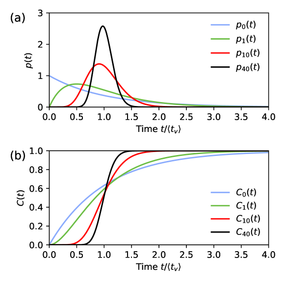
Fig 1: Representative probability distributions of vaccination time. (a) The distributions studied in this work, see eq. 42 with expected vaccination time ${\left\langle t_{v}\right\rangle}=(n+1)\tau$ for $n=0$, $1$, $10$, $40$, for arbitrary $\tau$. (b) The corresponding cumulative distribution functions, as defined by eq. 24.

Previously, we pointed out that vaccination uncertainty plays the role of a generalised form of discounting. For $p(t)=p_{0}(t)=\frac{1}{\tau}\exp[-t/\tau]$ and $C(t)=C_{0}(t)=1-\exp[-t/\tau]$, this reduces further to standard exponential discounting: With the utility integrand $u$ including a discounting factor $e^{-t/{\tau_{econ}}}$ as given in eq. 7, the utility function becomes

$$\tilde{U}= \ \int_{0}^{t_{e}}e^{-t/\tau}\left[u(\kappa(t),k(t))-U_{v}(t)\right]\,\mathrm{d}t+U_{e}$$

$$\tilde{U}_{e}= \ -\alpha\frac{\psi_{s,e}}{s_{e}}i_{e}M_{0}(t_{e},{\tau_{econ}},\eta,p(t))$$

$$\ -\alpha\left(\psi_{i,e}-i_{e}\frac{\psi_{s,e}}{s_{e}}\right)M_{0}(t_{e},{\tau_{econ}},1,p(t))$$ (44)

with

$$M_{0}(t_{e},{\tau_{econ}},\eta,\tau)=$$ (45)

$$e^{-t_{e}/\tau_{econ}}\left(1+\frac{1}{\tau/{\tau_{econ}}+\tau}\right)\frac{e^{-t_{e}/\tau}}{{1/{\tau_{econ}}}+\eta+1/\tau}$$ (46)

see SI, section C. This can be simplified further by introducing a new discounting time $\tilde{\tau}_{econ}$ and a modified cost of infection $\tilde{\alpha}$, obtaining

$$\tilde{U} =\int_{0}^{t_{e}}\tilde{u}(\kappa(t),k(t))\,\mathrm{d}t+\tilde{U}_{e}$$ (47)

$$\tilde{u} =e^{-t/\tilde{\tau}_{econ}}\left[-\tilde{\alpha}\>\psi_{i}-\beta\psi_{s}(\kappa-\kappa^{*})^{2}\right]$$ (48)

$$\tilde{\tau}_{econ} =\left(\frac{1}{\tau}+\frac{1}{\tau_{econ}}\right)^{-1}$$ (49)

$$\tilde{\alpha} =\alpha\left(1+\frac{1}{\tau/{\tau_{econ}}+\tau}\right)$$ (50)

$$\tilde{U}_{e} =-\tilde{\alpha}e^{-t_{e}/\tilde{\tau}_{econ}}\Big{[}\frac{\psi_{s,e}}{s_{e}}i_{e}\,\left(\frac{1}{1/\tilde{\tau}_{econ}+\eta}\right)$$ (51)

$$\ \ \ \ \ +\left(\psi_{i,e}-i_{e}\frac{\psi_{s,e}}{s_{e}}\right)\,\left(\frac{1}{1/\tilde{\tau}_{econ}+1}\right)\Big{]}$$ (52)

which yields boundary conditions for the values

$$v_{s}(t_{e})= \ \frac{\partial\tilde{U}_{e}}{\partial\psi_{s,e}}$$ (53)

$$= \ -\tilde{\alpha}e^{-t_{e}/\tilde{\tau}_{econ}}\frac{i_{e}}{s_{e}}\left(\frac{1}{1/\tilde{\tau}_{econ}+\eta}-\frac{1}{1/\tilde{\tau}_{econ}+1}\right)$$ (54)

$$v_{i}(t_{e})= \ \frac{\partial\tilde{U}_{e}}{\partial\psi_{i,e}}=-\frac{\tilde{\alpha}e^{-t_{e}/\tilde{\tau}_{econ}}}{1/\tilde{\tau}_{econ}+1}$$ (55)

These have the same form as the original equations, eqs. 7, 8 and 9, except for the salvage term $\tilde{U}_{e}$ and the boundary conditions for the economic value $v_{s}(t_{e})$. This small difference is usually negligible and vanishes when $t_{e}$ is chosen much larger than the duration of the epidemic, since $i_{e}$ is decaying exponentially for long times, see SI, section C. We had introduced the cutoff time $t_{e}$ only for numerical convenience anyway, and in order to accurately represent the full vaccination distribution $p(t)$, we choose it large enough such that it has no discernible effect on the dynamics, $t_{e}=200$. In that case one can then safely assume that $v_{s}(t_{e})\approx 0$ and the value boundary conditions become equivalent to the case of standard exponential discounting as well. Except for extremely small $\tau$, one can also approximate $\tilde{\alpha}=\alpha$.

Results

Individual decision making for known vaccination time

We numerically solve the resulting set of equations, eqs. 2, 13, 14 and 17, with a standard forward-backward sweep approach [27]. We ignore economic discounting by setting ${\tau_{econ}}\to\infty$.

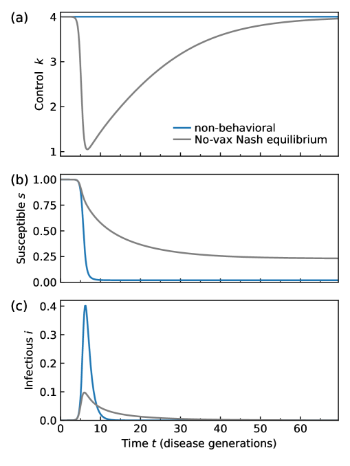
Fig S2: Self-organised social distancing slows down epidemics and reduces the total number of cases. (a) Nash equilibrium behaviour $k$ without the expectation of a vaccine becoming available ever (blue) as compared to the non-behavioural situation in which the behaviour is unchanged from the pre-pandemic behaviour, $k=\kappa^{*}$. The corresponding courses of the epidemic are shown in panel (b) for the susceptibles and (c) for the infected.

We show the Nash equilibrium behaviours and corresponding courses of the epidemic for a range of vaccination times $t_{v}$ in fig. 2(a-c). We choose here a cost of infection of $\alpha=400$, for which equilibrium social distancing slows down the duration of the epidemic from about 10 disease generations assuming no behavioural modification (see fig. S2 and Ref. [20]) to about 50 if there is no expectation of a vaccination (see curve labeled “no vax”). The peak of the epidemic occurs after 5-10 disease generations. The “no-vax” behaviour also is observed if the vaccine is expected to arrive far later than the course of the epidemic, e.g. see the data for $t_{v}=100$.

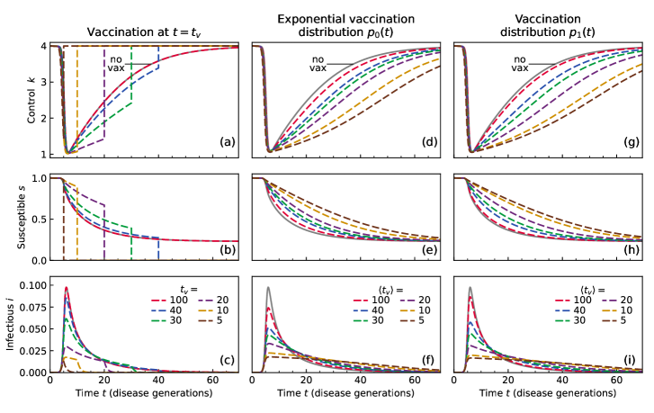
Fig 2: Self-organised social distancing is the stronger the sooner the vaccination date is expected. (a) Nash equilibrium behaviour $k$ for a range of sharp vaccination times $t_{v}$, as given in the legend of panel (c). The behaviour is insensitive to $t_{v}$ for large values and indistinguishable from the behaviour if the vaccination is not expected to occur. When $t_{v}$ is comparable to or shorter than the duration of the epidemic without vaccination, equilibrium behaviour exhibits strong social distancing. The corresponding courses of the epidemic are shown in panel (b) for the susceptibles and (c) for the infected. (d-f) Nash equilibrium behaviour $\tilde{k}$ and course of the epidemic assuming that the vaccination arrival time is exponentially distributed, $p=p_{0}(t)$, see eq. 42, with an expected vaccination time $\langle t_{v}\rangle$, see panel (f) for legend. The behaviour and corresponding course of epidemic arising from the assumption that vaccination will not occur are shown as gray solid lines. This is calculated from the case for precisely known vaccination time $t_{v}$ but with $t_{v}\to\infty$. (g-i) Nash equilibrium behaviour $\tilde{k}$ and course of the epidemic assuming that the vaccination arrival time is distributed according to $p_{1}$, see eq. 42. See panel (i) for legend. Other parameters, here and for all other shown data: infection cost $\alpha=400$ and no economic discounting, ${\tau_{econ}}\to\infty$.

If the vaccine arrives earlier, it begins to influence decision making, with social distancing becoming the more pronounced the earlier the vaccination is known to occur. The observed behaviour is quite similar to earlier results, see [11, 14]. The main difference is given by our different choice of parameters: the higher baseline infectivity $\kappa^{*}$ and higher cost of infection $\alpha$ lead to stronger social distancing which is gradually relaxed over a long time.

The equilibrium behaviour is especially sensitive to values of $t_{v}$ that are shorter than the duration of the “no-vax” rational epidemic course, indicating that it is not rational to further prolong the duration of the epidemic to hold out for the arrival of vaccine. We can conclude that the vaccination is only of relevance to the population if it is expected to happen on a shorter timescale than the duration of the epidemic itself.

Having established this result, we can now investigate how equilibrium behaviour is modified if the precise vaccination time is unknown.

Individual decision making for vaccination time distributions

The results presented below are numerical solutions of eqs. 2, 31, 35, 37, 40 and 94 with the same standard forward-backward sweep approach [27] as used for the sharp vaccination timing. In practice, however, we find that it is necessary to first introduce a rescaling of the economic values to avoid problems with numerical divergences, see SI, section D for details. We stress again that we calculate the equilibrium behaviour given a certain vaccination probability distribution $p(t)$ for any given time $t$ on the condition that vaccination has not yet occurred at that time. A vaccinated individual would exhibit behaviour $k=\kappa^{*}$. To facilitate comparison of the results for different probability distributions with each other, we present the results with respect to the expected vaccination time ${\left\langle t_{v}\right\rangle}=(n+1)\tau$ and not $\tau$ directly.

In comparison to the cases with precisely known vaccination time, the equilibrium behaviour for $p=p_{0}$ varies more evenly with $\langle t_{v}\rangle$, see fig. 2 (d-f). It is however still qualitatively similar in that shorter $\langle t_{v}\rangle$ encourages stronger social distancing. Even for very large $\langle t_{v}\rangle$, e.g. $\langle t_{v}\rangle=100$, we observe increased social distancing with respect to the no-vaccination case owing to the fact that the vaccination probability distribution at early times is non-zero. We also note that even for $t>{\left\langle t_{v}\right\rangle}$, i.e. when the vaccination event is overdue, there still exists an incentive to social distance more strongly than in the no-vaccination scenario.

For $p(t)=p_{1}(t)$, the results are qualitatively similar to those for $p_{0}$, see fig. 2 (g-i), even though the probability distribution looks quite different, exhibiting a peak. It stands to reason that the sharper peaked the probability distribution is, the closer the behaviour would match the situation in which the vaccination time is precisely known. This effect can be clearly observed in the expected number of vaccinations ${\left\langle s(t_{v})\right\rangle}=\int_{0}^{\infty}s(t_{v})p(t_{v})dt_{v}$, see fig. 3. For a sharp vaccination time $t_{v}$, this quantity is given by $s(t_{v})$, as already discussed. For the studied vaccination distributions, we observe that the more weakly varying the distribution is, i.e. the smaller $n$ is, the more smoothly ${\left\langle s(t_{v})\right\rangle}$ depends on ${\left\langle t_{v}\right\rangle}$. For $n=40$, the outcome already closely matches the case of sharp vaccination timing.

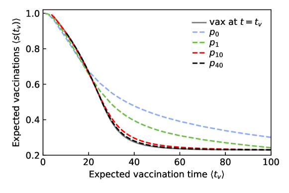
Fig 3: The number of expected vaccinations decreases with the expected vaccination time. Here we show the fraction of the population that is vaccinated $s(t_{v})$ for the equilibrium solution if the vaccination is known to occur at a precise $t_{v}$ in grey. The later the expected vaccination time, the smaller $s(t_{v})$ becomes. For comparison, we are showing the expected number of vaccinations, given by the expectation value of the susceptible compartment, ${\left\langle s\right\rangle}$ as a function of the expected vaccination time ${\left\langle t_{v}\right\rangle}$ for the a range of vaccination time distributions. The sharper the probability distribution (the higher the $n$), the more closely the result approaches the case of certain vaccination at $t=t_{v}$.

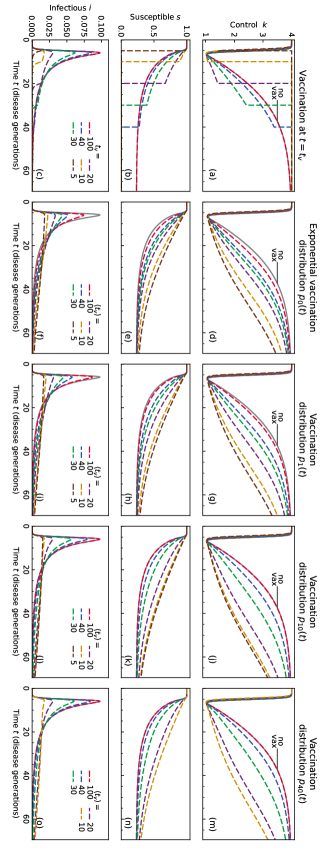
Fig S3: Self-organised social distancing is the stronger the sooner the vaccination date is expected. (a) Nash equilibrium behaviour for a range of sharp vaccination times $t_{v}$, as given in the legend of panel (c). The behaviour is insensitive to $t_{v}$ for large values and indistinguishable from the behaviour if the vaccination is not expected to occur. When $t_{v}$ is comparable to or shorter than the duration of the epidemic without vaccination, equilibrium behaviour exhibits strong social distancing. The corresponding courses of the epidemic are shown in panel (b) for the susceptibles and (c) for the infected. (d-f) Nash equilibrium behaviour and course of the epidemic assuming that the vaccination arrival time is exponentially distributed, $p=p_{0}(t)$, see eq. 42, with an expected vaccination time $\langle t_{v}\rangle$, see panel (f) for legend. The behaviour and corresponding course of epidemic arising from the assumption that vaccination will not occur are shown as grey solid lines. This is calculated from the case for precisely known vaccination time $t_{v}$ but with $t_{v}\to\infty$. (g-o) Same as (d-f) but for vaccination time distributions $p_{1}$, $p_{9}$, $p_{50}$, see eq. 42. Other parameters, here and for all other shown data: constant infection cost $\alpha=400$, and no economic discounting, ${\tau_{econ}}\to\infty$.

Noting that all studied distributions yield (almost) the same ${\left\langle s(t_{v})\right\rangle}$ at ${\left\langle t_{v}\right\rangle}=20$, we chose to compare the corresponding equilibrium behaviour directly, see fig. 4. Given the strongly different underlying probability distributions, the equilibrium behaviour has to be quite different to achieve a similar value of expected vaccinations: The more sharply peaked the vaccination distribution, the more stringent the observed social distancing is. The full data for $p_{10}$ and $p_{40}$ is shown in fig. S3.

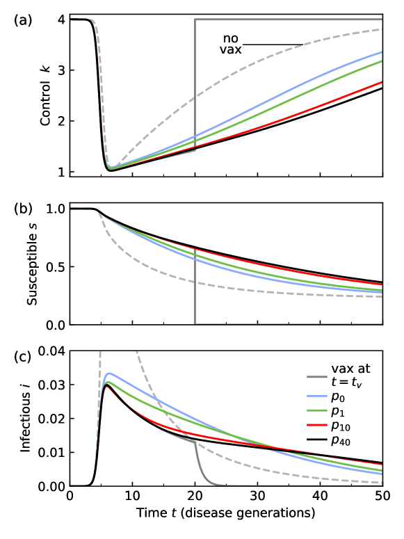
Fig 4: Social distancing is sensitive to distribution of the vaccination time. (a) Nash equilibrium behaviour $k$ for a range of vaccination time distributions $p_{n}$, as given in the legend of panel (c), all with expected vaccination time ${\left\langle t_{v}\right\rangle}=20$. For reference, we show the equilibrium behaviour if vaccination is not expected to occur (dashed line labelled “no vax”). Even though the expected vaccination time is similar, and the expected no. of vaccinations is (almost) the same, see fig. 3, we observe that significant social distancing occurs for longer durations with increasing sharpness $n$ of the vaccination distribution. The corresponding courses of the epidemic are shown in panel (b) for the susceptibles and (c) for the infectious (the “no vax” case peaks at $\max(i)\approx 0.1$).

Conclusion and discussion

Here, we have shown how the expectation of a future vaccination event influences social distancing behaviour in an epidemic. The earlier the vaccination is expected to happen and the more precisely the timing of the vaccination is known, the stronger the incentive to socially distance. In particular, the equilibrium social distancing only meaningfully deviates from the no-vaccination equilibrium behaviour if the vaccine is expected to arrive before the epidemic would have run its course under equilibrium social distancing.

As for the interpretation of our work in relation to previous works: In the special case of sharp vaccination timing, our results qualitatively reproduced the equilibrium results reported in [11, 14]. It had previously been reported for a scenario with uncertain vaccination arrival times that there would be little equilibrium behavioural modification [15]. This can be explained as follows: the vaccination probability distribution is modeled such that the vaccination arrival is equally likely for all times, resulting in severe uncertainty about the arrival time. In addition, the expected vaccination arrival time corresponds to the end of the epidemic under no-vaccination equilibrium social distancing. For that situation we also find very little additional social distancing. (They do find that vaccination affects influences government policy, an effect which we do not study here.)

Finally, we have demonstrated that if the vaccination time is exponentially distributed, it can be absorbed into an exponential discounting term with the time scale given by the expected vaccination time and can be interpreted as such. In general, we propose that any uncertainty in the vaccination time be interpreted as a form of generalised discounting.

We believe these results provide meaningful guidance to people and governmental decision makers for navigating epidemics. In particular, our work relates to how one should communicate vaccination development schedules. Since higher certainty about the vaccination arrival time during the epidemic leads to higher equilibrium social distancing, we suggest that such schedules should be communicated to the public as early and clearly as possible. In addition, it is important that vaccines are made available before the epidemic would have run its course under no-vaccination social distancing. Otherwise the vaccine itself does not serve as further incentive to the public for additional social distancing.

Supporting Information

A

Utility salvage term for vaccination at a precisely known time

In case a vaccine becomes available at $t_{v}$ and immediately protects every susceptible individual, we have $s(t>t_{v})=0$ and $\psi_{s}(t>t_{v})=0$. The SIR dynamics of eq. 2 then reduce to

$$\dot{i} =-i$$ (56)

Therefore, the population of infectious $i(t_{v})=i_{v}$ recover as

$$i(t>t_{v})=i_{v}\exp[-(t-t_{v})]$$ (57)

and likewise for the individual dynamics

$$\psi_{i}(t>t_{v})=\psi_{i,v}\exp[-(t-t_{v})]$$ (58)

Since there is no danger of becoming newly infected after $t_{v}$, there is no reason to modify one’s behaviour, $\kappa(t)=\kappa^{*}$. Taking the utility defined by eq. 7

$$U =\int_{0}^{\infty}u(t)dt\text{ with}$$

$$u =e^{-t/{\tau_{econ}}}\left[-\alpha\>\psi_{i}(t)-\beta\psi_{s}(\kappa(t)-\kappa^{*})^{2}\right]$$

we identify the late time utility coming from $t>t_{v}$ as

$$U_{v}=-\int_{t_{v}}^{\infty}e^{-t/{\tau_{econ}}}\alpha\psi_{i}\,\mathrm{d}t$$ (59)

This can be immediately integrated to yield

$$U_{v}=-\frac{e^{t_{v}/{\tau_{econ}}}\alpha\psi_{i,v}}{{1/{\tau_{econ}}}+1}$$ (60)

and the boundary conditions are therefore

$$v_{s}(t_{v})= \ \frac{\partial U_{v}}{\partial\psi_{s,v}}=0$$ (61)

$$v_{i}(t_{v})= \ \frac{\partial U_{v}}{\partial\psi_{i,v}}=-\frac{e^{t_{v}/{\tau_{econ}}}\alpha}{{1/{\tau_{econ}}}+1}$$ (62)

Assuming Nash equilibrium, the salvage term reads

$$U_{v}=-\frac{e^{t_{v}/{\tau_{econ}}}\alpha i_{v}}{{1/{\tau_{econ}}}+1}$$ (63)

B

Some calculations for special choices of vaccination distribution times

A relevant class of distributions of the vaccination time is

$$p_{n}(t)=\frac{t^{n}}{n!\tau^{n+1}}\exp[-t/\tau]$$ (64)

with integer exponent $n$ and decay time $\tau$. The expectation value of these distributions is

$$\int_{0}^{\infty}tp_{n}(t)\,dt=(n+1)\tau.$$ (65)

The probability distributions can also be written as

$$p_{n}(t)=\frac{1}{n!\tau^{n+1}}(-1)^{n}\frac{\partial^{n}}{\partial\sigma^{n}}\exp[-\sigma t]$$ (66)

and setting $\sigma=1/\tau$ afterwards . Introducing the appropriate differential operator $O_{n}$, which only acts on $\sigma$,

$$O_{n}=\frac{1}{n!\tau^{n+1}}(-1)^{n}\frac{\partial^{n}}{\partial\sigma^{n}}$$ (67)

we rewrite this

$$p_{n}(t)=O_{n}\exp[-\sigma t]$$ (68)

Then the cumulative distribution function can be written as

$$C_{n}(t) =\int_{0}^{t}p_{n}(t^{\prime})\,\mathrm{d}t^{\prime}=O_{n}\int_{0}^{t}\exp[-\sigma t^{\prime}]\,\mathrm{d}t^{\prime}$$ (69)

$$=O_{n}\left[\frac{1}{\sigma}(1-\exp[-\sigma t])\right]$$ (70)

and then setting $\sigma=1/\tau$. The operator has the convenient property that

$$O_{n}\left(\frac{1}{\sigma}\right)=\frac{1}{n!\tau^{n+1}}(-1)^{n}\frac{\partial^{n}}{\partial\sigma^{n}}\frac{1}{\sigma}=\frac{1}{(\tau\sigma)^{n+1}}=1$$ (71)

for $\sigma=1/\tau$. With this, we can see out that

$$C_{n}(t) =O_{n}\left[\frac{1}{\sigma}-\frac{1}{\sigma}\exp[-\sigma t]\right]=1-O_{n}\left[\frac{1}{\sigma}\exp[-\sigma t]\right]$$ (72)

$$=1-\frac{1}{n!\tau^{n+1}}\exp[-\sigma t]\frac{n!}{\sigma^{n+1}}\sum_{l=0}^{n}\frac{\sigma^{l}t^{l}}{l!}$$ (73)

$$=1-\exp[-t/\tau]\sum_{l=0}^{n}\frac{t^{l}}{l!\tau^{l}}$$ (74)

Hence, we can write

$$\frac{p_{n}(t)}{1-C_{n}(t)} =\frac{\frac{t^{n}}{n!\tau^{n+1}}\exp[-t/\tau]}{\exp[-t/\tau]\sum_{l=0}^{n}\frac{t^{l}}{l!\tau^{l}}}=\frac{t^{n}}{n!\tau^{n+1}}\left(\sum_{l=0}^{n}\frac{t^{l}}{l!\tau^{l}}\right)^{-1}$$ (75)

which for $t=0$ evaluates to $0$ and for late times tends to

$$\lim_{t\to\infty}\frac{p_{n}(t)}{1-C_{n}(t)} =\frac{1}{\tau}$$ (76)

C

Late time asymptotics

Here, we will calculate the asymptotic solution for the population compartments $s$ and $i$, the individual probabilities of being in said compartments $\psi_{s}$ and $\psi_{i}$, the relevant terms featuring their adjoint values $v_{i}$ and $(v_{s}-v_{i})$, as well as the Nash equilibrium behaviour $\kappa$ for late times in order to be able to calculate the salvage term for the utility.

We note that our interest lies in the case where the parameter of the vaccination probability distributions $\sigma=1/\tau>0$. This enforces that the distributions have well-defined means.

In the following, we restrict ourselves to vaccination probability distributions as defined by eq. 42. However, the calculations hold for any vaccination distribution $p(t_{v})$ which decays exponentially for large $t_{v}$.

In order to calculate the asymptotic solution for the population level SIR dynamics for late times, we expand the equations of eq. 2 according to $s(t)=s_{\infty}+\delta s(t)$, $i=\delta i(t)$, and $k(t)=\kappa^{*}-\delta k(t)$, with the $\delta$-quantities assumed to be small and focus on the most important $s$ and $i$ equations to first order in smallness. Rewriting eq. 2 leads to

$$\dot{\delta}s =-(s_{\infty}+\delta s)(\kappa^{*}-\delta k)\delta i$$ (77)

$$\dot{\delta}i =[(s_{\infty}+\delta s)(\kappa^{*}-\delta k)-1]\delta i$$ (78)

The necessary boundary conditions are given by $\delta s(t_{e})=\delta s_{e}=s_{e}-s_{\infty}$ and $\delta i(t_{e})=\delta i_{e}\equiv i_{e}$ for some late enough time $t_{e}$.

Assuming that the $\delta$-quantities are small, the first line of eq. 78 immediately reduces to

$$\dot{\delta}s =-s_{\infty}\kappa^{*}\delta i$$ (79)

In the second line of eq. 78, we can drop the terms which are quadratic in $\delta$-quantities

$$\dot{\delta}i =[(s_{\infty}\kappa^{*}-1)+\delta s\,\kappa^{*}-s_{\infty}\,\delta k]\delta i,$$ (80)

This equation involves a quantity

$$\eta=1-s_{\infty}\kappa^{*}\text{ with }0<\eta\leq 1,$$ (81)

The case $\eta=0$ occurs only in the limit $\alpha\to\infty$ and we only consider finite values of $\alpha$ in what follows. In order to confirm that

$$\frac{|\delta s\kappa^{*}-s_{\infty}\delta k|}{\eta}\ll 1$$ (82)

we will later demonstrate in a self-consistent way that $\delta k$ indeed decays asymptotically to 0 with the same exponent as $\delta i$ and $\delta s$. We numerically confirm that the inequality holds for $t_{e}$ and its corresponding $s_{e}$ and $i_{e}$ for the results presented in this work. Within this assumption, we write

$$\dot{\delta}s =-(1-\eta)\delta i$$ (83)

$$\dot{\delta}i =-\eta\delta i$$ (84)

The SIR variables therefore do not depend on $\delta k$ to leading order. The differential equations can be integrated to find

$$\delta s = c\frac{1-\eta}{\eta}\exp[-\eta t]$$ (85)

$$\delta i = c\exp[-\eta t]$$ (86)

with constant of integration $c$. Matching conditions at $t=t_{e}$, written $s(t_{e})=s_{e}$ and $i(t_{e})=i_{e}=\delta i_{e}$, we have

$$s_{e}-s_{\infty}\equiv\delta s_{e} = c\frac{1-\eta}{\eta}\exp[-\eta t_{e}]$$ (87)

$$\delta i_{e} = c\exp[-\eta t_{e}]$$ (88)

We can solve these two equations for the two unknowns $c$ and $\eta$ in terms of the two “terminal” quantities $s_{e}$ and $i_{e}$. Eliminating $c$ from Eq 88 yields

$$\eta=\frac{1}{\delta s_{e}/\delta i_{e}+1}$$ (89)

Hence $c=i_{e}\exp[\eta t_{e}]$ and we can write more simply

$$\delta s =\frac{1-\eta}{\eta}i_{e}\exp[-\eta(t-t_{e})]$$ (90)

$$\delta i =i_{e}\exp[-\eta(t-t_{e})]$$ (91)

In order to determine the value of $s_{\infty}$ (also contained in the definition of $\eta$), we evaluate $\delta s$ at $t_{e}$

$$s_{e}-s_{\infty}=\frac{1-\eta}{\eta}i_{e}=\frac{s_{\infty}\kappa^{*}}{1-s_{\infty}\kappa^{*}}i_{e}$$ (92)

and solve this quadratic equation in $s_{\infty}$,

$$s_{\infty} =\frac{1+(s_{e}+i_{e})\kappa^{*}-\sqrt{\left[1+(s_{e}+i_{e})\kappa^{*}\right]^{2}-4\kappa^{*}s_{e}}}{2\kappa^{*}}$$ (93)

Requiring that $s_{\infty}<1/\kappa^{*}$, we have selected the negative branch. Hence

$$\eta= \ \frac{1-(s_{e}+i_{e})\kappa^{*}+\sqrt{\left[1+(s_{e}+i_{e})\kappa^{*}\right]^{2}-4\kappa^{*}s_{e}}}{2}$$ (94)

Next, we calculate the asymptotic solution for the individual dynamics. We have $\psi_{s}(t)=\psi_{s,\infty}+\delta\psi_{s}(t)$, $\psi_{i}(t)=\delta\psi_{i}(t)$, and $\kappa(t)=\kappa^{*}-\delta\kappa(t)$, assuming that the $\delta$-quantities are all of the same order of smallness. To first order in smallness eq. 4

$$\dot{\psi}_{s} =-\kappa\psi_{s}i$$ (95)

$$\dot{\psi}_{i} =\kappa\psi_{s}i-\psi_{i}$$

becomes

$$\dot{\delta\psi_{s}} =-\psi_{s,\infty}\kappa^{*}\delta i$$ (96)

$$\dot{\delta\psi_{i}} =\psi_{s,\infty}\kappa^{*}\delta i-\delta\psi_{i}$$ (97)

The condition for this expansion to be valid is eq. 82, the same as for eq. 84, because in the Nash equilibrium $\psi_{s}=s$. The “terminal” quantities $\psi_{s,e}$ and $\psi_{i,e}$ can be used as boundary conditions: $\delta\psi_{s}(t_{e})=\psi_{s,e}-\psi_{s,\infty}$ and $\delta\psi_{i}(t_{e})=\psi_{i,e}$. We obtain as solutions

$$\delta\psi_{s}(t)= \ \frac{\psi_{s,\infty}\kappa^{*}}{\eta}i_{e}e^{-\eta(t-t_{e})}$$ (98)

$$\delta\psi_{i}(t)= \ \frac{\psi_{s,\infty}}{s_{\infty}}i_{e}e^{-\eta(t-t_{e})}$$ (99)

$$\ +\left(\psi_{i,e}-i_{e}\frac{\psi_{s,\infty}}{s_{\infty}}\right)e^{-(t-t_{e})}$$ (100)

We can determine $\psi_{s,\infty}$ by evaluating eq. 98 at $t_{e}$, i.e. $\psi_{s,e}-\psi_{s,\infty}=\delta\psi_{s}(t_{e})$, and solving for $\psi_{s,\infty}$

$$\psi_{s,\infty}=\psi_{s,e}\frac{\eta}{\eta+i_{e}\kappa^{*}}$$ (101)

With this and eq. 92, we can show that

$$\frac{\psi_{s,e}}{\psi_{s,\infty}} =\frac{\eta+i_{e}\kappa^{*}}{\eta}=1+\frac{\kappa^{*}}{1-s_{\infty}\kappa^{*}}i_{e}$$ (102)

$$=\frac{1}{s_{\infty}}\left(s_{\infty}+\frac{s_{\infty}\kappa^{*}}{1-s_{\infty}\kappa^{*}}i_{e}\right)=\frac{s_{e}}{s_{\infty}}$$ (103)

$$\Rightarrow\frac{\psi_{s,\infty}}{s_{\infty}}=\frac{\psi_{s,e}}{s_{e}}$$ (104)

The asymptotic solutions then read

$$\delta\psi_{s}(t)= \ \psi_{s,e}\frac{i_{e}\kappa^{*}}{\eta+i_{e}\kappa^{*}}e^{-\eta(t-tf)}$$ (105)

$$\delta\psi_{i}(t)= \ \frac{\psi_{s,e}}{s_{e}}i_{e}e^{-\eta(t-tf)}$$ (106)

$$\ +\left(\psi_{i,e}-i_{e}\frac{\psi_{s,e}}{s_{e}}\right)e^{-(t-t_{e})}$$ (107)

The complete asymptotic solution is therefore given by eqs. 91, 105 and 107, with definitions eqs. 81 and 93.

Utility salvage term from asymptotic solution, Nash equilibrium, without vaccination

For later reference, we calculate the salvage term arising from integrating out the optimal utility for $t>t_{e}$ with the asymptotic solution, in the case that no vaccination ever happens. Taking the utility defined by eq. 7

$$U =\int_{0}^{\infty}u(t)dt\text{ with}$$

$$u =e^{-t/{\tau_{econ}}}\left[-\alpha\>\psi_{i}(t)-\beta\psi_{s}(\kappa(t)-\kappa^{*})^{2}\right]$$

we identify the late time utility coming from $t>t_{e}$ as

$$U_{e}=-\int_{t_{e}}^{\infty}e^{-t/{\tau_{econ}}}\left[\alpha\delta\psi_{i}+\beta(\psi_{s,\infty}+\delta\psi_{s})\delta\kappa^{2}\right]dt$$ (108)

We note that in leading order of smallness, the $\delta\kappa^{2}$ term can be left out and that we therefore have

$$U_{e}= \ -\alpha\int_{t_{e}}^{\infty}e^{-t^{\prime}/{\tau_{econ}}}\delta\psi_{i}(t^{\prime})\>dt^{\prime}$$ (109)

$$\delta\psi i(t^{\prime})= \ \frac{\psi_{s,e}}{s_{e}}i_{e}e^{-\eta(t^{\prime}-t_{e})}+\left(\psi_{i,e}-i_{e}\frac{\psi_{s,e}}{s_{e}}\right)e^{-(t^{\prime}-t_{e})}$$

from eq. 107 and eq. (91). Hence

$$U_{e} =-\alpha\frac{\psi_{s,e}}{s_{e}}i_{e}e^{\eta t_{e}}\int_{t_{e}}^{\infty}e^{-({1/{\tau_{econ}}}+\eta)t^{\prime}}\>dt^{\prime}$$ (110)

$$-\alpha\left(\psi_{i,e}-i_{e}\frac{\psi_{s,e}}{s_{e}}\right)e^{t_{e}}\int_{t_{e}}^{\infty}e^{-({1/{\tau_{econ}}}+1)t^{\prime}}\>dt^{\prime}$$ (111)

This integrates to

$$U_{e}= \ -e^{t_{e}/{\tau_{econ}}}\alpha\ \times$$ (112)

$$\left(\frac{i_{e}}{{1/{\tau_{econ}}}+\eta}\,\frac{\psi_{s,e}}{s_{e}}+\frac{1}{{1/{\tau_{econ}}}+1}\left(\psi_{i,e}-i_{e}\frac{\psi_{s,e}}{s_{e}}\right)\right)$$

From this, we can now calculate the boundary conditions for the value equations

$$v_{s}(t_{e})= \ \frac{\partial U_{e}}{\partial\psi_{s,e}}$$ (113)

$$= -e^{t_{e}/{\tau_{econ}}}\alpha\ \frac{i_{e}}{s_{e}}\left(\frac{1}{{1/{\tau_{econ}}}+\eta}\,-\frac{1}{{1/{\tau_{econ}}}+1}\right)$$ (114)

$$v_{i}(t_{e})= \ \frac{\partial U_{e}}{\partial\psi_{i,e}}=-e^{t_{e}/{\tau_{econ}}}\alpha\ \frac{1}{{1/{\tau_{econ}}}+1}$$ (115)

Finally, we are able to assume Nash equilibrium, so that $\psi_{s,e}=s_{e}$ and $\psi_{i,e}=i_{e}$. The salvage term then simplifies to

$$U_{f}= \ -e^{t_{e}/{\tau_{econ}}}\alpha\ \frac{i_{e}}{{1/{\tau_{econ}}}+\eta}$$

Utility salvage term for a distribution of vaccination times

Taking the utility defined by eq. 27

$$\tilde{U} =\int_{0}^{\infty}[1-C(t)]\,u+p(t)\,U_{v}(t)\,\mathrm{d}t$$

with $u$ as defined in eq. 7

$$u=e^{-t/{\tau_{econ}}}\left[-\alpha\>\psi_{i}(t)-\beta\psi_{s}(\kappa(t)-\kappa^{*})^{2}\right]$$

and $U_{v}$ as defined in eq. 60

$$U_{v}(t)=-e^{-t/{\tau_{econ}}}\alpha\ \frac{\psi_{i}(t)}{{1/{\tau_{econ}}}+1}$$

we identify the late time utility coming from $t>t_{e}$ as

$$\tilde{U}_{e}=\int_{t_{e}}^{\infty}[1-C(t)]\,u+p(t)\,U_{v}(t)\,\mathrm{d}t$$ (116)

Having obtained the asymptotic optimal solution, we are now in the position to explicitly calculate this salvage term. In terms of the small $\delta$-quantities we get

$$\tilde{U}_{e}=\int_{t_{e}}^{\infty} \Big{[}[1-C(t)]\,e^{-t/{\tau_{econ}}}\left[-\alpha\>\delta\psi_{i}(t)-\beta(\psi_{s,\infty}+\delta\psi_{s})\delta\kappa^{2}\right]$$

$$-p(t)\,e^{-t/{\tau_{econ}}}\alpha\ \frac{\delta\psi_{i}(t)}{{1/{\tau_{econ}}}+1}\Big{]}\,\mathrm{d}t$$

We note that in leading order of smallness, the $\delta\kappa^{2}$ term can be left out and that we therefore have

$$\tilde{U}_{e} =-\alpha\int_{t_{e}}^{\infty}e^{-t/{\tau_{econ}}}\left(1-C(t)+\frac{p(t)}{{1/{\tau_{econ}}}+1}\right)\delta\psi_{i}(t)\,\mathrm{d}t$$ (117)

$$\delta\psi_{i}(t) =\frac{\psi_{s,e}}{s_{e}}i_{e}e^{-\eta(t-t_{e})}+\left(\psi_{i,e}-i_{e}\frac{\psi_{s,e}}{s_{e}}\right)e^{-(t-t_{e})}$$ (118)

with the asymptotic solution matched to the state of the system at $t_{e}$. Introducing the helper function

$$M(t_{e},{\tau_{econ}},\eta,p(t))=$$ (119)

$$\ \int_{t_{e}}^{\infty}e^{-\eta(t-t_{e})}e^{-t/{\tau_{econ}}}\left(1-C(t)+\frac{p(t)}{{1/{\tau_{econ}}}+1}\right)\,\mathrm{d}t$$

we can write

$$\tilde{U}_{e}= \ -\alpha\frac{\psi_{s,e}}{s_{e}}i_{e}M(t_{e},{\tau_{econ}},\eta,p(t))$$ (120)

$$\ -\alpha\left(\psi_{i,e}-i_{e}\frac{\psi_{s,e}}{s_{e}}\right)M(t_{e},{\tau_{econ}},1,p(t))$$ (121)

Now the boundary conditions for the values can be written as

$$v_{s}(t_{e})= \ \frac{\partial\tilde{U}_{e}}{\partial\psi_{s,e}}$$ (122)

$$= \ -\alpha\frac{i_{e}}{s_{e}}\left[M(t_{e},{\tau_{econ}},\eta,p(t))-M(t_{e},{\tau_{econ}},1,p(t))\right]$$ (123)

$$v_{i}(t_{e})= \ \frac{\partial\tilde{U}_{e}}{\partial\psi_{i,e}}=-\alpha M(t_{e},{\tau_{econ}},1,p(t))$$ (124)

In the Nash equilibrium, the utility captured by the salvage term can be more simply calculated as

$$\tilde{U}_{e}= \ -\alpha\,i_{e}M(t_{e},{\tau_{econ}},\eta,p(t)).$$ (125)

As before, we choose $p$ and $C$ to be of the form

$$p_{n}(t) =O_{n}\exp[-\sigma t]$$ (126)

$$C_{n}(t) =O_{n}\left[\frac{1}{\sigma}(1-\exp[-\sigma t])\right]$$ (127)

with $O_{n}=\frac{1}{n!\tau^{n+1}}(-1)^{n}\frac{\partial^{n}}{\partial\sigma^{n}}$, see eqs. 67, 68 and 70, and then setting $\sigma=1/\tau$ in the end. Focusing on the integral for now and exploiting again that $1-O_{n}(1/\sigma)=0$ when $\sigma=1/\tau$, we can write

$$M_{n}(t_{e},{\tau_{econ}},\eta,\tau)\equiv M(t_{e},{\tau_{econ}},\eta,p_{n}(t))$$ (128)

$$=e^{\eta t_{e}}O_{n}\left[\left(\frac{1}{\sigma}+\frac{1}{{1/{\tau_{econ}}}+1}\right)\int_{t_{e}}^{\infty}e^{-({1/{\tau_{econ}}}+\eta)t}e^{-\sigma t}\,\mathrm{d}t\right]$$ (129)

$$=e^{-t_{e}/\tau_{econ}}O_{n}\left[\frac{{1/{\tau_{econ}}}+1+\sigma}{\sigma({1/{\tau_{econ}}}+1)}\frac{e^{-\sigma t_{e}}}{{1/{\tau_{econ}}}+\eta+\sigma}\right]$$ (130)

Special case: For $n=0$, we have $O_{0}=1/\tau$ and therefore we find with setting $\sigma=1/\tau$ that

$$M_{0}(t_{e},{\tau_{econ}},\eta,\tau)$$ (131)

$$=e^{-t_{e}/\tau_{econ}}\left(1+\frac{1}{\tau({1/{\tau_{econ}}}+1)}\right)\frac{e^{-t_{e}/\tau}}{{1/{\tau_{econ}}}+\eta+1/\tau}$$

and

$$\tilde{U}_{e}= -\alpha e^{-t_{e}/\tau_{econ}}e^{-t_{e}/\tau}\left(1+\frac{1}{\tau({1/{\tau_{econ}}}+1)}\right)\times$$ (132)

$$\ \Bigg{[}\frac{\frac{\psi_{s,e}}{s_{e}}i_{e}}{{1/{\tau_{econ}}}+\eta+\frac{1}{\tau}}+\frac{\psi_{i,e}-i_{e}\frac{\psi_{s,e}}{s_{e}}}{{1/{\tau_{econ}}}+1+\frac{1}{\tau}}\Bigg{]}$$

We see that introducing $\tilde{\alpha}=\alpha(1+1/[\tau({1/{\tau_{econ}}}+1)])$ and $1/\tilde{\tau}_{econ}={1/{\tau_{econ}}}+1/\tau$ yield

$$\tilde{U}_{e} =-\tilde{\alpha}e^{-t_{e}/\tilde{\tau}_{econ}}\Big{[}\frac{\psi_{s,e}}{s_{e}}i_{e}\,\left(\frac{1}{1/\tilde{\tau}_{econ}+\eta}\right)$$ (133)

$$+\left(\psi_{i,e}-i_{e}\frac{\psi_{s,e}}{s_{e}}\right)\,\left(\frac{1}{\tilde{\tau}_{econ}+1}\right)\Big{]}$$ (134)

which is of the same form as eq. 112, demonstrating that for an exponential distribution of vaccination times, the problem can be restated as one without vaccination but with modified exponential discounting and modified cost of infection.

Self consistency

Now we can return to the question of whether we simplified the differential equations appropriately, by examining whether the asymptotic solution is consistent with all assumptions leading to its calculation. Specifically, we need to find criteria for $s_{e}$, $i_{e}$, $t_{e}$ which guarantee that the conditions (i) $|\delta s|\ll s_{\infty}$, (ii) $|\delta k|\ll\kappa^{*}$ and (iii) $|\delta s\kappa^{*}-s_{\infty}\delta k|\ll\eta$ hold for all $t>t_{e}$, noting that $\delta\kappa=\delta k$ in the Nash equilibrium. In practice, when we solve the optimal control problem on the domain $0\leq t\leq t_{e}$ for a certain $t_{e}$, we confirm that the three criteria are satisfied by the obtained numerical solution.

Condition (i): Self-consistently, $\delta s(t)\ll s_{\infty}$ will always hold for large enough times $t$. We observe that eq. 92 provides an upper bound for $\delta s(t)$ for all $t>t_{e}$. Thus we must require that

$$1\gg\frac{\delta s}{s_{\infty}}=\frac{s_{\infty}\kappa^{*}}{\eta s_{\infty}}i_{e}=\frac{\kappa^{*}}{\eta}i_{e}$$ (135)

and therefore

$$i_{e}\ll\frac{\eta(s_{e},i_{e})}{\kappa^{*}}$$ (136)

Condition (ii): Some reasoning on whether $\delta k$ and $\delta\kappa$ are small: In the Nash equilibrium both are given by, see eq. 17,

$$\delta k =\delta\kappa=-\frac{1}{2\beta}\frac{e^{t/{\tau_{econ}}}}{1-C(t)}(v_{s}-v_{i})i$$ (137)

From hereon, we only mention $\delta k$, with $\delta\kappa$ implied to be equal. Without making any assumptions about $v_{s}$ and $v_{i}$ at this point, we have at leading order,

$$\delta k =\frac{1}{2\beta}\frac{e^{t/{\tau_{econ}}}}{1-C(t)}(v_{s}-v_{i})\delta i$$ (138)

To determine whether $\delta k$ is of the same order of smallness as $\delta i$ or not, we need to obtain the asymptotic solution for $(v_{s}-v_{i})$. Since we can obtain an analytic solution for $v_{i}$, we discuss it first. The value $v_{i}$ follows eq. 35

$$\dot{v}_{i}=e^{-t/{\tau_{econ}}}\alpha\left[1-C(t)+\frac{p(t)}{{1/{\tau_{econ}}}+1}\right]+v_{i}$$ (139)

In the domain $t_{e}\leq t<\infty$, the relevant boundary condition is at $t\to\infty$ and corresponds to $\lim_{t\to\infty}v_{i}(t)=0$ since there is no corresponding salvage term. The analytic solution for $v_{i}$, as defined by eq. 35 can be calculated as follows, if we restrict ourselves to the probability distributions defined as $p_{n}$. First we insert the operator forms of $p$ and $C$, eqs. 68 and 70

$$\dot{v}_{i} =e^{-t/{\tau_{econ}}}\alpha\left[1+O_{n}\left[\frac{1}{\sigma}(\exp[-\sigma t]-1)\right]+\frac{O_{n}\exp[-\sigma t]}{{1/{\tau_{econ}}}+1}\right]$$ (140)

$$+v_{i}$$ (141)

with

$$O_{n}=\frac{1}{n!\tau^{n+1}}(-1)^{n}\frac{\partial^{n}}{\partial\sigma^{n}}$$ (142)

We note again that $O_{n}(1/\sigma)=1$ when we set $\sigma=1/\tau$. Therefore we can write

$$\dot{v}_{i} =v_{i}+e^{-t/{\tau_{econ}}}\alpha\,O_{n}\left[\frac{1}{\sigma}\exp[-\sigma t]+\frac{\exp[-\sigma t]}{{1/{\tau_{econ}}}+1}\right]$$ (143)

$$=v_{i}+e^{-t/{\tau_{econ}}}\alpha\,O_{n}\left[e^{-\sigma t}\left(\frac{1}{\sigma}+\frac{1}{{1/{\tau_{econ}}}+1}\right)\right]$$ (144)

Abbreviating with a coefficient $A$ which only depends on parameters $\tau$, $\sigma$ and ${\tau_{econ}}$

$$A=\frac{1}{\sigma}+\frac{1}{{1/{\tau_{econ}}}+1}=\frac{{1/{\tau_{econ}}}+1+\sigma}{\sigma({1/{\tau_{econ}}}+1)}$$ (145)

we can write more concisely

$$\dot{v}_{i} =v_{i}+e^{-t/{\tau_{econ}}}\alpha\,O_{n}\left[e^{-\sigma t}A\right]$$ (146)

We can make an ansatz with an integrating factor $g(t)$

$$\frac{\partial}{\partial t}[v_{i}g]=\dot{v}_{i}g+\dot{g}v_{i}=ge^{-t/{\tau_{econ}}}\alpha\,O_{n}\left[e^{-\sigma t}A\right]$$ (147)

such that

$$\dot{v}_{i}+\frac{\dot{g}}{g}v_{i}=e^{-t/{\tau_{econ}}}\alpha\,O_{n}\left[e^{-\sigma t}A\right]$$ (148)

Therefore $\dot{g}/g=-1$ from which we conclude

$$g=e^{-t}$$ (149)

Returning to the original ansatz

$$\frac{\partial}{\partial t}[v_{i}e^{-t}]=e^{-t}e^{-t/{\tau_{econ}}}\alpha\,O_{n}\left[e^{-\sigma t}A\right]$$ (150)

We can integrate this to

$$v_{i}e^{-t} =\alpha\,O_{n}\int_{\infty}^{t}e^{-t^{\prime}}e^{t^{\prime}/{\tau_{econ}}}e^{-\sigma t^{\prime}}A\,\mathrm{d}t^{\prime}$$ (151)

$$=-\alpha\,O_{n}\Big{[}\frac{e^{-t}e^{-t/{\tau_{econ}}}e^{-\sigma t}A}{1+{1/{\tau_{econ}}}+\sigma}\Big{]}$$ (152)

For the definite integral as written the constant of integration vanishes, since we know that $v_{i}(t)\to 0$ for $t\to\infty$. Therefore we have the analytic solution for the value of being infectious (after reinserting $A$)

$$v_{i} =-\alpha\,e^{-t/{\tau_{econ}}}O_{n}\Bigg{[}\frac{e^{-\sigma t}}{\sigma({1/{\tau_{econ}}}+1)}\Bigg{]}$$ (153)

This equation holds even in the limit of ${\tau_{econ}}\to\infty$ because our interest lies in the case where $\sigma=1/\tau>0$. Asymptotically for large times, we observe that

$$v_{i}(t)\sim e^{-(1/{\tau_{econ}}+1/\tau)t}$$ (154)

Next, we calculate an asymptotic solution for $\bar{v}\equiv v_{s}-v_{i}$, using eq. 35

$$\dot{\bar{v}}= \ \dot{v}_{s}-\dot{v}_{i}$$ (155)

$$= \ -\frac{\partial\tilde{H}}{\partial\psi_{s}}$$ (156)

$$= \ [1-C(t)]e^{-t/{\tau_{econ}}}\beta(\kappa-\kappa^{*})^{2}+\bar{v}\kappa i$$ (157)

$$\ -e^{-t/{\tau_{econ}}}\alpha\left[1-C(t)+\frac{p(t)}{{1/{\tau_{econ}}}+1}\right]-v_{i}$$ (158)

$$= \ \frac{1-C(t)}{e^{t/{\tau_{econ}}}}\beta\delta\kappa^{2}+\bar{v}(\kappa^{*}-\delta\kappa)\delta i$$ (159)

$$\ -e^{-t/{\tau_{econ}}}\alpha\left[1-C(t)+\frac{p(t)}{{1/{\tau_{econ}}}+1}\right]-v_{i}$$ (160)

In the domain $t_{e}\leq t<\infty$, the relevant boundary condition on $v_{s}$ and $v_{i}$ is at $t\to\infty$ and corresponds to $\lim_{t\to\infty}v_{s}(t)=\lim_{t\to\infty}v_{i}(t)=0$ since there is no corresponding salvage term. Therefore $\lim_{t\to\infty}\bar{v}(t)=0$. Inserting the eq. 138 for $\delta\kappa$, we obtain

$$\dot{\bar{v}}= \ \frac{1-C(t)}{e^{t/{\tau_{econ}}}}\beta\left(\frac{1}{2\beta}\frac{e^{t/{\tau_{econ}}}}{1-C(t)}\bar{v}\delta i\right)^{2}$$ (161)

$$\ +\bar{v}\left(\kappa^{*}-\frac{1}{2\beta}\frac{e^{t/{\tau_{econ}}}}{1-C(t)}\bar{v}\delta i\right)\delta i$$ (162)

$$\ -e^{-t/{\tau_{econ}}}\alpha\left[1-C(t)+\frac{p(t)}{{1/{\tau_{econ}}}+1}\right]-v_{i}$$ (163)

$$= \ \frac{1}{4\beta}\frac{e^{t/{\tau_{econ}}}}{1-C(t)}\bar{v}^{2}\delta i^{2}+\bar{v}\left(\kappa^{*}-\frac{1}{2\beta}\frac{e^{t/{\tau_{econ}}}}{1-C(t)}\bar{v}\delta i\right)\delta i$$ (164)

$$\ -e^{-t/{\tau_{econ}}}\alpha\left[1-C(t)+\frac{p(t)}{{1/{\tau_{econ}}}+1}\right]-v_{i}$$ (165)

$$= \ \bar{v}\delta i\left(\kappa^{*}+\frac{1}{2\beta}\frac{e^{t/{\tau_{econ}}}}{1-C(t)}\bar{v}\delta i\right)$$ (166)

$$\ -e^{-t/{\tau_{econ}}}\alpha\left[1-C(t)+\frac{p(t)}{{1/{\tau_{econ}}}+1}\right]-v_{i}$$ (167)

By referring to eqs. 64 and 74, we find that asymptotically

$$e^{-t/{\tau_{econ}}}\alpha\left[1-C(t)+\frac{p(t)}{{1/{\tau_{econ}}}+1}\right]\sim e^{-t/{\tau_{econ}}}e^{-t/\tau}$$ (169)

which is the same behaviour as exhibited by $v_{i}$, see eq. 154. Since asymptotically the exponential terms will dominate, we can conclude, by using eq. 91,

$$\dot{\bar{v}}\sim \ \bar{v}e^{-\eta t}\left(\kappa^{*}+e^{(1/{\tau_{econ}}+1/\tau-\eta)t}\bar{v}\right)-e^{-(1/{\tau_{econ}}+1/\tau)t}$$ (170)

To satisfy this equation, $\bar{v}$ has to behave as

$$\dot{\bar{v}}\sim\bar{v}\sim e^{-(1/{\tau_{econ}}+1/\tau)t}$$ (171)

since then

$$e^{-(1/{\tau_{econ}}+1/\tau)t}$$ (172)

$$\sim\ e^{-(1/{\tau_{econ}}+1/\tau)t}e^{-\eta t}\left(\kappa^{*}+e^{(1/{\tau_{econ}}+1/\tau-\eta)t}e^{-(1/{\tau_{econ}}+1/\tau)t}\right)$$ (173)

$$-e^{-(1/{\tau_{econ}}+1/\tau)t}$$ (174)

$$\sim\ e^{-(1/{\tau_{econ}}+1/\tau)t}[e^{-\eta t}\left(\kappa^{*}+e^{-\eta t}\right)-1]$$ (175)

which is satisfied for late times at which $\exp[-\eta t]$ can be considered small. Inserting this result into the expression for $\delta k$, eq. 138, and using eqs. 64, 74 and 91 we obtain

$$\delta k\sim\frac{e^{t/{\tau_{econ}}}}{e^{-t/\tau}}e^{-(1/{\tau_{econ}}+1/\tau)t}e^{-\eta t}\sim e^{-\eta t}$$ (177)

Thus $\delta k$ is asymptotically of comparable smallness to $\delta i$ and $\delta s$. As a concrete criterion, we numerically confirm that $\delta k(t_{e})\ll\kappa^{*}$ holds for all our numerically obtained results.

Condition (iii): For the simplification of eq. 80 into eq. 84 to hold, we must require that

$$\frac{|\delta s\,\kappa^{*}-s_{\infty}\,\delta\kappa|}{|s_{\infty}\kappa^{*}-1|}\ll 1$$ (178)

Having confirmed that $\delta s$ and $\delta\kappa=\delta k$ eventually become smaller than any given positive bound, it suffices to test for this after we have numerically solved the control problem.

D

Rescaling the values

In eq. 40, we observe that the term $e^{t/{\tau_{econ}}}/(1-C(t))$ diverges for $t\to\infty$ with the divergence being compensated by the values. Numerically, this is challenging to handle. Similarly to how it is common practice to introduce the current value Hamiltonian and to absorb the economic discounting into its corresponding current-values, we absorb the diverging terms into the values. We define

$$\hat{v}_{s}=\frac{e^{t/{\tau_{econ}}}}{1-C(t)}v_{s},\ \ \ \hat{v}_{i}=\frac{e^{t/{\tau_{econ}}}}{1-C(t)}v_{i}$$ (179)

and obtain new differential equations for them using eq. 35

$$\frac{\partial}{\partial t}{\hat{v}}_{s} =\frac{\frac{1}{{\tau_{econ}}}e^{t/{\tau_{econ}}}}{1-C(t)}v_{s}+\frac{e^{t/{\tau_{econ}}}p(t)}{(1-C(t))^{2}}v_{s}+\frac{e^{t/{\tau_{econ}}}}{1-C(t)}\dot{v}_{s}$$ (180)

$$=\left(\frac{1}{{\tau_{econ}}}+\frac{p(t)}{1-C(t)}\right)\hat{v}_{s}$$ (181)

$$\ \ \ +\frac{e^{t/{\tau_{econ}}}}{1-C(t)}[1-C(t)]e^{-t/{\tau_{econ}}}\beta(\kappa-\kappa^{*})^{2}+(\hat{v}_{s}-\hat{v}_{i})\kappa i$$ (182)

$$=\left(\frac{1}{{\tau_{econ}}}+\frac{p(t)}{1-C(t)}\right)\hat{v}_{s}+\beta(\kappa-\kappa^{*})^{2}+(\hat{v}_{s}-\hat{v}_{i})\kappa i$$ (183)

$$\frac{\partial}{\partial t}{\hat{v}}_{i} =\left(\frac{1}{{\tau_{econ}}}+\frac{p(t)}{1-C(t)}\right)\hat{v}_{i}+\frac{e^{t/{\tau_{econ}}}}{1-C(t)}\times$$ (184)

$$\ \ \left(e^{-t/{\tau_{econ}}}\alpha\left[1-C(t)+\frac{p(t)}{{1/{\tau_{econ}}}+1}\right]+v_{i}\right)$$ (185)

$$=\left(\frac{1}{{\tau_{econ}}}+\frac{p(t)}{1-C(t)}\right)\hat{v}_{i}+\hat{v}_{i}$$ (186)

$$\ \ +\alpha\left[1+\frac{p(t)}{1-C(t)}\frac{{\tau_{econ}}}{1+{\tau_{econ}}}\right]$$ (187)

with boundary conditions

$$\hat{v}_{s}(t_{e})= \ -\alpha\frac{i_{e}}{s_{e}}\left[\hat{M}(t_{e},{\tau_{econ}},\eta,p)-\hat{M}(t_{e},{\tau_{econ}},1,p)\right]$$ (188)

$$\hat{v}_{i}(t_{e})= \ -\alpha\hat{M}(t_{e},{\tau_{econ}},1,p)$$ (189)

with helper function

$$\hat{M}(t_{e},{\tau_{econ}},\eta,p)=\frac{e^{t_{e}/{\tau_{econ}}}e^{\eta t_{e}}}{1-C(t_{e})}\times$$ (190)

$$\int_{t_{e}}^{\infty}e^{-\eta t}e^{-t/{\tau_{econ}}}\left(1-C(t)+\frac{p(t)}{{1/{\tau_{econ}}}+1}\right)\,\mathrm{d}t$$ (191)

Then we can rewrite eq. 40 more simply

$$\tilde{\kappa}=\kappa^{*}-\frac{1}{2\beta}(\hat{v}_{s}-\hat{v}_{i})i$$ (192)

References

- 1. Roush SW, Murphy TV, Basket MM, Iskander JK, Moran JS, Seward JF, et al. Historical comparisons of morbidity and mortality for vaccine-preventable diseases in the United States. Journal of the American Medical Association. 2007;298(18):2155–2163. doi:10.1001/jama.298.18.2155.
- 2. Keeling MJ, Moore S, Penman BS, Hill EM. The impacts of SARS-CoV-2 vaccine dose separation and targeting on the COVID-19 epidemic in England. Nature Communications. 2023;14(1):1–10. doi:10.1038/s41467-023-35943-0.
- 3. Yan Y, Malik AA, Bayham J, Fenichel EP, Couzens C, Omer SB. Measuring voluntary and policy-induced social distancing behavior during the COVID-19 pandemic. Proceedings of the National Academy of Sciences of the United States of America. 2021;118(16):1–9. doi:10.1073/pnas.2008814118.
- 4. Wang Z, Bauch CT, Bhattacharyya S, D’Onofrio A, Manfredi P, Perc M, et al. Statistical physics of vaccination. Physics Reports. 2016;664:1–113. doi:10.1016/j.physrep.2016.10.006.
- 5. Ferguson NM, Cummings DAT, Fraser C, Cajka JC, Cooley PC, Burke DS. Strategies for mitigating an influenza pandemic. Nature. 2006;442(7101):448–452. doi:10.1038/nature04795.
- 6. Tanimoto J. Social Dilemma Analysis of the Spread of Infectious Disease. In: Evolutionary Games with Sociophysics. Springer, Singapore; 2018. p. 155–216. Available from: http://link.springer.com/10.1007/978-981-13-2769-8_4.
- 7. Mellacher P. COVID-Town: An Integrated Economic-Epidemiological Agent-Based Model. Graz Schumpeter Centre; 2020. 23.
- 8. Chandrasekhar AG, Goldsmith-Pinkham P, Jackson MO, Thau S. Interacting regional policies in containing a disease. Proceedings of the National Academy of Sciences of the United States of America. 2021;118(19):1–7. doi:10.1073/pnas.2021520118.
- 9. Holme P, Saramäki J. Temporal networks. Physics Reports. 2012;519(3):97–125. doi:10.1016/j.physrep.2012.03.001.
- 10. Holme P, Masuda N. The basic reproduction number as a predictor for epidemic outbreaks in temporal networks. PLoS ONE. 2015;10(3):1–15. doi:10.1371/journal.pone.0120567.
- 11. Reluga TC. Game Theory of Social Distancing in Response to an Epidemic. PLoS Comput Biol. 2010;6(5):e1000793. doi:10.1371/journal.pcbi.1000793.
- 12. Reluga TC, Galvani AP. A general approach for population games with application to vaccination. Math Biosci. 2011;230(2):67–78. doi:10.1016/j.mbs.2011.01.003.
- 13. Fenichel EP, Castillo-Chavez C, Ceddia MG, Chowell G, Parra PAG, Hickling GJ, et al. Adaptive human behavior in epidemiological models. Proc Natl Acad Sci. 2011;108(15):6306–6311. doi:10.1073/pnas.1011250108.
- 14. Makris M, Toxvaerd F. Great Expectations : Social Distancing in Anticipation of Pharmaceutical Innovations; 2020. 2097. Available from: https://www.repository.cam.ac.uk/handle/1810/315201.
- 15. Eichenbaum MS, Rebelo S, Trabandt M. The Macroeconomics of Epidemics. Review of Financial Studies. 2021;34(11):5149–5187. doi:10.1093/rfs/hhab040.
- 16. McAdams D. Nash SIR: An Economic-Epidemiological Model of Strategic Behavior During a Viral Epidemic. Covid Economics. 2020;doi:10.2139/ssrn.3593272.
- 17. Toxvaerd F. Rational Disinhibition and Externalities in Prevention. International Economic Review. 2019;60(4):1737–1755. doi:10.1111/iere.12402.
- 18. Rowthorn R, Toxvaerd F. The optimal control of infectious diseases via prevention and treatment. University of Cambridge; 2020. 2027.
- 19. Bethune ZA, Korinek A. COVID-19 infection externalities: trading off lives vs. livelihoods. Cambridge, MA: National Bureau of Economic Research; 2020. 27009.
- 20. Schnyder SK, Molina J, Yamamoto R, Turner MS. Rational social distancing policy during epidemics with limited healthcare capacity. under review. 2022;doi:10.48550/arXiv.2205.00684.
- 21. Toxvaerd F, Rowthorn R. On the management of population immunity. University of Cambridge; 2020. 2080.
- 22. Grauer J, Löwen H, Liebchen B. Strategic spatiotemporal vaccine distribution increases the survival rate in an infectious disease like Covid-19. Scientific Reports. 2020;10(1):1–10. doi:10.1038/s41598-020-78447-3.
- 23. Augsburger IB, Galanthay GK, Tarosky JH, Rychtář J, Taylor D. Imperfect vaccine can yield multiple Nash equilibria in vaccination games. Mathematical Biosciences. 2023;356(December 2022):108967. doi:10.1016/j.mbs.2023.108967.
- 24. Schwarzendahl FJ, Grauer J, Liebchen B, Löwen H. Mutation induced infection waves in diseases like COVID-19. Scientific Reports. 2022;12(1):1–11. doi:10.1038/s41598-022-13137-w.
- 25. Acemoglu D, Chernozhukov V, Werning I, Whinston MD. Optimal targeted lockdowns in a multi-group SIR model. National Bureau of Economic Research; 2020. 27102. Available from: http://www.nber.org/papers/w27102.
- 26. Kermack WO, McKendrick AG. A contribution to the mathematical theory of epidemics. Proceedings of the Royal Society of London Series A, Containing Papers of a Mathematical and Physical Character. 1927;115(772):700–721. doi:10.1098/rspa.1927.0118.
- 27. Lenhart S, Workman J. Optimal Control Applied to Biological Models. Chapman and Hall/CRC; 2007.