Morphological Sampling Theorem and its Extension to Grey-value Images

Abstract

Sampling is a basic operation in image processing. In classic literature, a morphological sampling theorem has been established, which shows how sampling interacts by morphological operations with image reconstruction. Many aspects of morphological sampling have been investigated for binary images, but only some of them have been explored for grey-value imagery.

With this paper, we make a step towards completion of this open matter. By relying on the umbra notion, we show how to transfer classic theorems in binary morphology about the interaction of sampling with the fundamental morphological operations dilation, erosion, opening and closing, to the grey-value setting. In doing this we also extend the theory relating the morphological operations and corresponding reconstructions to use of non-flat structuring elements. We illustrate the theoretical developments at hand of examples.

1 Introduction

Mathematical morphology is a very successful approach in image processing, cf. Serra-Soille ; Najman-Talbot ; Roerdink-2011 for an account. Morphological filters make use of a so called structuring element (SE). The SE is characterised by shape, size and centre location. There are two types of SEs, flat and non-flat r1 . A flat SE defines a neighbourhood of the centre pixel where morphological operations take place. A non-flat SE may additionally contain finite values used as additive offsets. The basic morphological operations are dilation and erosion. In a discrete setting as discussed in this work, these operations are realized by setting a pixel value to the maximum or minimum of the discrete image function within the SE centred upon it, respectively. The fundamental building blocks dilation and erosion may be combined to many morphological processes of practical interest, like e.g. opening, closing or top hats.

Sampling is a basic operation in signal and image processing. The celebrated Nyquist-Shannon sampling theorem relates the bandwidth of a continuous-scale signal to its reconstruction via equidistant sampled values, cf. Shannon-1998 for an account. Turning to morphological filters, the classic sampling theorem has an analogon within the framework of discrete sets and lattices. In this setting, the proceeding is based on image reconstruction by using samples together with the standard morphological processes of dilation and erosion as well as their combinations; see the classic works of Haralick and co-authors r2 ; Haralick88 as well as previous developments in r1 . In these works, sampling on the image grid was put in relation with image reconstruction via dilation and closing, and formulated in r2 as the digital morphological sampling theorem.

Considering the literature that followed the seminal work r2 on morphological sampling, we are not aware of further elaborations on sampling issues related to morphological filters. To the best of our knowledge the results documented in r2 have been cited for giving a theoretical basis for different developments, but they have not been continued at exactly that point. However, in the mentioned work several mathematical assertions related to sampling and its interaction with the basic morphological processes dilation, erosion opening and closing have been addressed only for binary images, while they have not been carried over to the setting of grey value imagery. More precisely, this open issue refers to the situation when filtering morphologically in the sampled domain, i.e., making use of a sampled account of a given image. This is from a computational point of view an interesting setting since the image dimension and thus the amount of necessary filtering operations may be reduced by sampling considerably.

In the same line of classic works, the relation between morphological operations and reconstruction of grey-value images was explored in the context of max-pooling in r3 . Let us note that the max-pooling operation as introduced in ZC-88 is often used in convolutional neural networks Goodfellow-et-al-2016 .

Let us elaborate a bit more at this point. While r3 presents relations between operating morphologically before sampling and morphologically operating in the sampled domain, there are several limitations by the proceeding in r3 , so that it represents an important step in the investigation of morphological operations in context of sampling and reconstruction, but it is not a complete theory. First, the theory in r3 is limited to a particular type of sampling, i.e. max-pooling. Max-pooling is the dilation by a square flat SE followed by sampling, i.e., dilation is used in a first step as a filter before the sampling step. Reconstruction is also obtained in r3 by dilation. Since dilation is not an idempotent operation, it is seldom used directly as a filter in real world applications, and a corresponding sampling and reconstruction setting as in r3 bears considerable restrictions. Let us also note that the work r3 assumes that the SE is already a subset of the sampled domain, i.e., technically the SE is affected by and acts on only those pixels of the image which are sampled. Finally, the work in r3 is limited to flat filters and SEs. The discussions are limited to the lattice-algebraic framework r4 , which lacks the tools to work with non-flat morphology.

Let us also elaborate a little more on the latter aspect in order to clarify the nature of our proposed extensions upon aforementioned classic works. The lattice algebraic theory provides a rich framework to study mathematical morphology, see e.g. r4 ; r5 . Lattice theory examines morphological operations as transformations on the complete lattice group of images. The ordering within the lattice is based on the inherent ordering, whether partial or total, of the pixel values, which, in the case of grey-value images, is the total order of the set of integers that make up the grey values. To summarize, lattice theory is largely based on tonal relationship between pixels. However, the lattice theory in itself lacks effective tools to deal with non-flat SEs and sampling. In particular, it largely neglects the spatial relationship between pixels of an image and the pixels of an SE as it moves across the image during morphological operations. The constraints imposed by lattice theory on the study of grey-value morphological sampling are apparent in r3 , where the authors attempt to employ this approach. Firstly, the filters and S.Es are restricted to be flat. Moreover, the SE is already in the sampled domain, that is, the action of SE on the pixels of the image which are sampled is unaffected by the image pixels which are not sampled.

To overcome the aforementioned limitations, we employ the umbra formulation of grey-value images. Umbra technique allows us to treat morphological operations on $N$-dimensional grey-value images (by flat or non-flat SEs) as binary morphological operations of their corresponding $(N+1)$-dimensional umbras r1 . Binary morphology is in turn founded on the spatial arrangement of pixels. Its basic operations are set operations, where both the binary image and SE are treated as sets of positional vectors. Furthermore, r2 thoroughly examines the connection between binary morphology and sampling.

Our Contributions. In a previous conference paper sridhar-breuss-sampling-caip , we have shown that it is possible to extend the work in r3 to non-flat filters and SEs using umbra formulation of morphological operations, and we have proposed a few results that can be derived from r2 . More precisely, we explored an alternative definition of grey-scale opening and closing to prove reconstruction bounds for the interaction of sampling with these operations. In the current paper we build upon sridhar-breuss-sampling-caip and extend the classic work of Haralick et al. in r2 on digital morphological sampling of grey value images. As the main point of our developments, we formulate and prove theorems relating morphological operations, sampling and image reconstruction by dilation and closing. Let us point out again clearly, that corresponding results have been derived in a relatively simple way for binary images in r2 , but they have not been extended up to now to grey-value imagery. The theory we formulate is also used here to extend the work in r3 to non-flat morphology. In doing this, we give a theoretical foundation for specific uses of the max-pooling operation used in modern deep learning literature. In total, compared to sridhar-breuss-sampling-caip , we give a much more extensive account of the theoretical framework, proving in this context several additional results.

We believe that especially the extension to non-flat morphology may be an interesting point with respect to recent developments in incorporating morphological layers in neural networks, see for instance Shen-2019 ; Franchi-2020 ; Kirszenberg-2021 ; Hermary-2022 . There the learned morphological filters within the layers are usually non-flat. Thus we give a theoretical foundation of this recent machine learning technique by the current paper.

Paper Organisation. In the next section we briefly recall the classic notions from mathematical morphology for binary as well as grey value images, see for instance r1 ; Matheron-75 ; Serra-82 ; Serra-88 ; Soille-2003 for a corresponding account of the field and the basic notions underlying our work. In addition, we will briefly recall the digital morphological sampling theorem in the binary and grey value setting, respectively. The third section contains the main part of our new results. In the fourth section, we use the developed results to extend the theory in r3 to non-flat structuring elements. We visualize the meaning of theoretical developments by some experiments within the text. The paper is finished by concluding remarks.

2 Morphological Operations

As indicated we now recall formal definitions and some fundamental properties of morphological operations that help to assess the later developments.

2.1 Morphological Notions for Binary Images

Let $\mathbb{\mathchar 69\relax}$ denote the set of integers used to index the rows and column of the image. $\mathbb{\mathchar 69\relax}^{N}$ is a $N$-tuple of $\mathbb{\mathchar 69\relax}$. A (two dimensional)binary image $A$ is a subset of $\mathbb{\mathchar 69\relax}^{2}$. That is, if a vector $x\in A\subseteq\mathbb{\mathchar 69\relax}$, then the position at $x$ is a white dot, where the default background is black. For sake of generality, we consider the image as $A\subseteq\mathbb{\mathchar 69\relax}^{N}$, $N\in\mathbb{N}$ r1 .

Definition 1.

Translation, Dilation and Erosion, Reflection, Duality. Let $A$, $B$ be subsets of $\mathbb{\mathchar 69\relax}^{N}$. For $x\in\mathbb{\mathchar 69\relax}^{N}$, the translation of $A$ by $x$ is written as $(A)_{x}$ $=$ $\{c\in\mathbb{\mathchar 69\relax}^{N}|c=a+x\text{ for some }a\in A\}$. The dilation of $A$ by $B$ is defined as

$$\begin{split}A\oplus B&=\{c\in\mathbb{\mathchar 69\relax}^{N}|c=a+b\text{ for some }a\in A,b\in B\}\\ &=\bigcup_{b\in B}(A)_{b}\end{split}$$ (1)

The erosion of set $A$ by $B$ is defined as

$$\begin{split}A\ominus B&=\{x|x+b\in A\text{ for each }b\in B\}\\ &=\{x\in\mathbb{\mathchar 69\relax}^{N}|(B)_{x}\subseteq A\}\\ &=\bigcap_{b\in B}(A)_{-b}\end{split}$$ (2)

In addition, the reflection of a set $B$ is denoted by $\breve{B}=\{x|\text{ for some }b\in B\text{, }x=-b\}$. Moreover, it holds duality in the sense $(A\ominus B)^{c}=A^{c}\oplus\breve{B}$.

Opening and Closing as described below can be employed to erase image details smaller than the structuring element without distorting unsuppressed geometric features, see e.g. r1 . They can easily be generalised to the grey value setting.

Definition 2.

Opening and Closing, Duality of Opening and Closing. The opening of $B\subseteq\mathbb{\mathchar 69\relax}^{N}$ by structuring element $K$ is denoted by $B\circ K$ and is defined as $B\circ K=(B\ominus K)\oplus K$. Analogously, opening is denoted as $B\bullet K=(B\oplus K)\ominus K$. The operations are dual i.e. $(A\bullet B)^{c}=A^{c}\circ B$.

We note that there exist the following alternative definitions of opening and closing which are useful in proofs of various results:

$$\begin{split}A\circ B&=\{x\in A|\text{ for some }y\text{, }x\in B_{y}\subseteq A\}\\ &=\bigcup_{\{y|B_{y}\subseteq A\}}B_{y}\end{split}$$ (3)

and

$$\begin{split}A\bullet B&=\{x|x\in\breve{B_{y}}\text{ implies }\breve{B_{y}}\cap A\neq\emptyset\}\end{split}$$ (4)

Let us now give some comments on the meaning of the binary digital morphological sampling theorem at hand of an example, see Figure 1. As the corresponding sampling theorem will be recalled in detail for the grey-value setting, we refrain from giving a more detailed exposition here.

Figure 1: The sets $K$, $S$ and $B$ used as an example; $K$ is the underlying structuring element, and $S$ is the sampling sieve.

We observe that the sampling sieve $S$ as in the figure will return every second grid point after sampling. Fixing the centre point of the structuring element $K$ at the same pixel as the centre of the sampling sieve, we see that the range of the structuring element is smaller than the distance between grid points of the sampling sieve. This amounts for a correct sampling and can be used systematically for image reconstructions as documented by an example given in Figure 2.

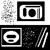
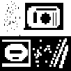
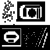
Figure 2: Binary example image, of size $102\times 102$, $F_{1}$ (left), its maximal reconstruction after sampling, $(F_{1}\cap S)\oplus K$, (centre) and its minimal reconstruction after sampling, $(F_{1}\cap S)\bullet K$, (right). For computing the maximal and minimal reconstruction, respectively, the original image $F_{1}$ has first been sampled by $F_{1}\cap S$, which may reduce effectively the resolution (to a quarter of the original one) as only every second pixel is taken into account in both grid directions, see $S$ in Figure 1. Then, by dilating with $K$ on the original grid, i.e. with the original resolution, we obtain as by the process of dilation an upper bound version of the original image called maximal reconstruction. The minimal reconstruction is obtained by closing the sample with $K$ on the original grid.

We now recall the binary version of the Digital Morphological Sampling Theorem from r2 .

Theorem 2.1.

(Binary Digital Morphological Sampling Theorem) Let $F,\>K,\>S\in\mathbb{\mathchar 69\relax}^{N}$, where $F$ is the binary image, $S$ is the sampling sieve and $K$ is the structuring element used for filtering. Suppose $S$ and $K$ satisfy the sampling conditions

1. $S\oplus S=S$

2. $S=\breve{S}$

3. $K\cap S=\{0\}$

4. $K=\breve{K}$

5. $a\in K_{b}\Rightarrow K_{a}\cap K_{b}\cap S\neq\emptyset$

Then,

1. $F\cap S\>=\>[(F\cap S)\bullet K]\cap S$

2. $F\cap S\>=\>[(F\cap S)\oplus K]\cap S$

3. $(F\cap S)\bullet K\>\subseteq F\bullet K$

4. $(F\cap S)\oplus K\>\supseteq F\circ K$

5. If $F=F\circ K=F\bullet K$, then $(F\cap S)\bullet K\>\subseteq F\>\subseteq(F\cap S)\oplus K$

6. If $A=A\circ K$ and $F\cap S=A\cap S$, then $A\supseteq\>(F\cap S)\oplus K\>\Rightarrow A=\>(F\cap S)\oplus K$

7. If $A=A\bullet K$ and $F\cap S=A\cap S$, then $A\subseteq\>(F\cap S)\bullet K\>\Rightarrow A=\>(F\cap S)\bullet K$

The conditions IV and V imply that $S\oplus K=\mathbb{\mathchar 69\relax}^{N}$. The condition III implies that $K$ is just smaller than two sampling intervals. The Morphological Sampling Theorem states how the image must be filtered (i.e. opened or closed by $K$) to preserve the relevant information after sampling and gives set bounding relationships on reconstruction of morphologically filtered images.

We now proceed by reproducing some results given in r3 on relation between sampling the binary image after performing morphological operations and morphologically operating in the sampled domain. These results will still be useful later in the grey value setting, as these are concerned with the underlying set on which the operations are performed.

Let us note that the set $B$ is the SE which is used to perform morphological operations on the image $F_{1}$. The example figures in this section demonstrate the relationship between morphologically operating on the image $F_{1}$ with $B$, sampling using sieve $S$ and filter $K$.

Some of the following results, e.g. Theorem 2.9 or Theorem 2.5, require that $B=B\circ K$. This in essence means that $B$ does not have any details (white region) finer than the filter $K$, and $B$ can be appropriately reconstructed from the sampled SE, $B\cap S$, as mentioned in the Binary Digital Morphological Sampling Theorem 2.1, cf. result V.

Proposition 2.2.

Let $B\subseteq\mathbb{\mathchar 69\relax}^{N}$ be the structuring element. Then

1. $(F\cap S)\oplus(B\cap S)\>\subseteq\>(F\oplus B)\cap S$

2. $(F\cap S)\ominus(B\cap S)\>\supseteq\>(F\ominus B)\cap S$

Figures 5 and 5 illustrate the first part of above proposition. Figures 8 and 8 illustrate the second part of the proposition.

Figure 3: $(F_{1}\oplus B)\cap S$ ABC ABCDE

Figure 4: $(F_{1}\cap S)\oplus(B\cap S)$ ABCDE

Figure 5: $\{[(F_{1}\cap S)\bullet K]\oplus B\}\cap S$

Figure 6: $(F_{1}\ominus B)\cap S$ ABC ABCDE

Figure 7: $(F_{1}\cap S)\ominus(B\cap S)$ ABCDE

Figure 8: $\{[(F_{1}\cap S)\oplus K]\ominus B\}\cap S$

Lemma 2.3.

1. $(F\cap S)\oplus(B\cap S)\>=\>[F\oplus(B\cap S)]\cap S$

2. $(F\cap S)\ominus(B\cap S)\>=\>[F\ominus(B\cap S)]\cap S$

Lemma 2.4.

Let $B=B\circ K$ . Then $[(F\cap S)\bullet K]\oplus B\subseteq\>[(F\cap S)\oplus K]\oplus(B\cap S)$

The following two theorems formulated in r2 , as indicated for binary images, elaborate on interaction of sampling and dilation/erosion, respectively. Let us note that these theorems serve as a motivation for proving and validating corresponding theorems in the grey value setting later.

Theorem 2.5.

Sample Dilation Theorem. Let $B=B\circ K$. Then $(F\cap S)\oplus(B\cap S)=\>\{[(F\cap S)\bullet K]\oplus B\}\cap S$

Theorem 2.6.

Sample Erosion Theorem. Let $B=B\circ K$ Then $(F\cap S)\ominus(B\cap S)=\>\{[(F\cap S)\oplus K]\ominus B\}\cap S$.

Notice that Figures 5 and 5 are identical. These figures demonstrate Sample Dilation Theorem 2.5, meaning that dilation in sampled domain (here, $(F_{1}\cap S)\oplus(B\cap S)$) is equivalent to sampling after dilation of the minimal reconstruction (here, $\{[(F_{1}\cap S)\bullet K]\oplus B\}\cap S$).

Similarly, Figures 8 and 8 are identical. This pair demonstrates Sample Erosion Theorem 2.6, meaning that erosion in sampled domain (here, $(F_{1}\cap S)\ominus(B\cap S)$) is equivalent to sampling after erosion of the maximal reconstruction (here, $\{[(F_{1}\cap S)\oplus K]\oplus B\}\cap S$).

Proposition 2.7.

$[F\circ(B\cap S)]\cap S=\>(F\cap S)\circ(B\cap S)$

Proposition 2.8.

$[F\bullet(B\cap S)]\cap S=(F\cap S)\bullet(B\cap S)$

Similarly to Theorems 2.5, 2.6, the following two theorems provide the interaction of two other fundamental morphological operations, closing and opening, with sampling. We will also extend the following result to the grey value setting.

Theorem 2.9.

Sample Opening and Closing Bounds Theorem. Suppose $B=B\circ K$, then

1. $\{F\circ[(B\cap S)\oplus K]\}\cap S\subseteq\>(F\cap S)\circ(B\cap S)\subseteq\>\{[(F\cap S)\oplus K]\circ B\}\cap S$

2. $\{[(F\cap S)\bullet K]\bullet B\}\cap S\subseteq\>(F\cap S)\bullet(B\cap S)\subseteq\>\{F\bullet[(B\cap S)\oplus K]\}\cap S$

Figures 11-11 demonstrate interaction of sampling with opening operation. We can observe that opening in the sampled domain is bounded above by sampling the opening of maximal reconstruction of image (here, $\{[(F_{1}\cap S)\oplus K]\circ B\}\cap S$) and bounded below by sampling of opening by maximal reconstruction of filter (here, $\{F_{1}\circ[(B\cap S)\oplus K]\}\cap S$).

In a similar way, Figures 14-14 demonstrate interaction of sampling with closing operation. We see that closing in sampled domain is bounded by sampling of closing minimal reconstruction of the image (here, $\{[(F_{1}\cap S)\bullet K]\bullet B\}\cap S$) and sampling of closing by maximal reconstruction of the filter (here, $\{F_{1}\bullet[(B\cap S)\oplus K]\}\cap S$).

Figure 9: $\{F_{1}\circ[(B\cap S)\oplus K]\}\cap S$ ABCDE

Figure 10: $(F_{1}\cap S)\circ(B\cap S)$ ABCDE

Figure 11: $\{[(F_{1}\cap S)\oplus K]\circ B\}\cap S$

Figure 12: $\{[(F_{1}\cap S)\bullet K]\bullet B\}\cap S$

Figure 13: $(F_{1}\cap S)\bullet(B\cap S)$ ABCDE

Figure 14: $\{F_{1}\bullet[(B\cap S)\oplus K]\}\cap S$

Theorem 2.10.

Sampling Opening And Closing Theorem. Suppose $B=B\circ K$.

1. If $F=(F\cap S)\oplus K$ and $B=(B\cap S)\oplus K$, then $(F\cap S)\circ(B\cap S)=\>(F\circ B)\cap S$

2. If $F=(F\cap S)\bullet K$ and $B=(B\cap S)\oplus K$, then $(F\cap S)\bullet(B\cap S)=\>(F\bullet B)\cap S$

2.2 Morphological Notions for Grey-value Images

Let $\mathbb{\mathchar 69\relax}$ be the set of integers used for denoting the indices of the coordinates. A grey-value image is represented by a function $f:F\rightarrow L$, $F\subseteq\mathbb{\mathchar 69\relax}^{N}$, $L=[0,l]$, where $l>0$ is the upper limit for grey values at a pixel in grey-value image, and $N=2$ for two dimensional grey-value images.

The SEs are of finite size. The morphological operations require taking $\max$ or $\min$ of grey values over finite sets (of pixels) in our setting. Therefore, the results are independent on whether $L$ is a discrete set (e.g., subset of integers) or a continuous set (e.g., sub-interval of real numbers).

The proposed extension of the previous notions to grey-value images requires to define the notions of top surfaces and the umbra of an image, compare r1 . Also see Figure 15 for the latter. In a first step we rely on both notions for defining dilation and erosion.

Definition 3.

Top Surface. Let $A\subseteq\mathbb{\mathchar 69\relax}^{N}\times L$. and $F=\{x\in\mathbb{\mathchar 69\relax}^{N}|\>\text{for some }y\in L,\>(x,y)\in A\}$. Then the top surface of $A$ is denoted as $T[A]$ and defined as $T[A](x)\>=\>\max\{y|\>(x,y)\in A\}$.

Definition 4.

Umbra of an Image. Let $F\subseteq\mathbb{\mathchar 69\relax}^{N}$ and $f:F\rightarrow L$. The umbra of the image $f$ is denoted by $U[f]$ and is defined as $U[f]=\>\{(x,y)|\>x\in F\text{, }y\in L\text{ and }0\leq y\leq f(x)\}$.

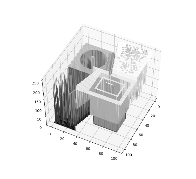
Figure 15: Left: An example grey-value image, of size $102\times 102$, $f:F\rightarrow L$ used for examples. Right: Visualisation of the corresponding umbra.

The umbra is useful for studying geometric relations between pixels, as it makes use of both spatial and tonal information. Thus, umbra approach provides important and convenient tools to deal with non-flat SEs and sampling, as already briefly discussed in the introduction. Using umbra allows us to describe grey-value morphological operations in terms of corresponding binary operations of umbra, making use of SE on umbra of the image. Thereby, the SE by itself is also transferred to the umbra setting. See Definition 5 for dilation, Definition 6 for erosion and Proposition 6 for opening and closing. In this way we are able to extend many morphological concepts developed for binary images directly to grey-value images.

Our definition of umbra, compare Figure 15, turns out to work perfectly well for grey-value images, compare r1 . Note that we restrict ourselves here to discrete non-negative pixel values at discrete positions (pixels). The underlying concept cannot be directly extended to continuous domain or negative values, compare r6 ; r7 .

Definition 5.

Dilation for Grey Value Images. Let $F,\>K\subseteq\mathbb{\mathchar 69\relax}^{N}$ and $f:F\rightarrow L$, $k:K\rightarrow L$. The dilation of $f$ by $k$ is denoted by $f\oplus k:\>F\oplus K\rightarrow L$ and is defined as $f\oplus k=\>T[U[f]\oplus U[k]]$.

Definition 6.

Erosion for Grey Value Images. Let $F,\>K\subseteq\mathbb{\mathchar 69\relax}^{N}$ and $f:F\rightarrow L$, $k:K\rightarrow L$. The erosion of $f$ by $k$ is denoted by $f\ominus k:\>F\ominus K\rightarrow L$ and is defined as $f\ominus k=\>T[U[f]\ominus U[k]]$.

As already mentioned, the operations of opening and closing can easily be extended from binary images to the grey-value setting, following the same combination of dilation/erosion as in Definition 2. That is, $f\circ k$ $=$ $(f\ominus k)\oplus k$ and $f\bullet k$ $=$ $(f\oplus k)\ominus k$. Similarly to the binary versions, grey-value opening and closing are anti-extensive and extensive, respectively. Both grey-value opening and closing are idempotent as well as dual operations.

Propositions 2.11 and 2.12 are used to compute dilation and erosion for a grey-value image.

Proposition 2.11.

Let $F,\>K\subseteq\mathbb{\mathchar 69\relax}^{N}$ and $f:F\rightarrow L$, $k:K\rightarrow L$. Then $f\oplus k:\>F\oplus K\rightarrow L$ can be computed by $(f\oplus k)(x)=\>\max_{u\in K,\>x-u\in F}{\{f(x-u)\>+\>k(u)\}}$.

Proposition 2.12.

Let $F,\>K\subseteq\mathbb{\mathchar 69\relax}^{N}$ and $f:F\rightarrow L$, $k:K\rightarrow L$. Then $f\ominus k:\>F\ominus K\rightarrow L$ can be computed by $(f\ominus k)(x)=\>\min_{u\in K}{\{f(x+u)\>-\>k(u)\}}$.

Let us note that the method to compute $(f\ominus k)(x)$ as given in Proposition 2.12 is valid only for $x$ such that $(x,y)\in U[f]\ominus U[k]$ for some $y$. To extend the definition to all $x\in F\ominus K$, one may define $(f\ominus k)(x)=\>\max\{0,\min_{u\in K}{\{f(x+u)\>-\>k(u)\}}\}$.

Suppose now $A$ and $B$ are umbras. Then $A\oplus B$ and $A\ominus B$ are umbras. The Umbra Homomorphism Theorem below makes this property precise.

Theorem 2.13.

Umbra Homomorphism Theorem. Let $F,\>K\subset\mathbb{\mathchar 69\relax}^{N}$ and $f:F\rightarrow L$ and $k:K\rightarrow L$. Then

1. $U[f\oplus k]=U[f]\oplus U[k]$

2. $U[f\ominus k]=U[f]\ominus U[k]$

We will employ at some point the following notions.

Definition 7.

Reflection of an Image. The reflection of a grey-value image $f:F\rightarrow L$ is denoted by $\breve{f}:\breve{F}\rightarrow L$, and it is defined as $\breve{f}(x)=f(-x)$ for each $x\in\breve{F}$.

Definition 8.

Negative of an Image. The negative of a grey-value image $f:F\rightarrow L$ is denoted by $-f:F\rightarrow L$, and it is defined as $(-f)(x)=l-f(x)$ for each $x\in F$, where $l>0$ is again the upper limit for possible grey values.

Let us note that Haralick r1 defines the negative of an image via $(-f)(x)=-f(x),x\in F$. Definition 8 as we propose above is more suitable for many purposes because the grey value at a pixel is not supposed to be negative.

We also recall the concept of boundedness for grey-value images. Let $f:F\rightarrow L$ and $g:G\rightarrow L$ be two grey-value images. We say $f\leq g$ if $F\subseteq G$ and $f(x)\leq g(x)$ for each $x\in F$.

Let us now recite the grey-value morphological sampling theorem from r2 .

Theorem 2.14.

The Grey Scale Digital Morphological Sampling Theorem. Let $F,K,S\subseteq\mathbb{\mathchar 69\relax}^{N}$, $f:F\rightarrow L$ is the image, $k:K\rightarrow L$ is the structuring element used for filtering. Let $K,S$, and $k:K\rightarrow L$ satisfy the following conditions:

1. $S\oplus S=S$

2. $S=\breve{S}$

3. $K\cap S=\{0\}$

4. $a\in K_{b}\Rightarrow K_{a}\cap K_{b}\cap S\neq\emptyset$

5. $k=\breve{k}$

6. $k(a)\leq k(a-b)+k(b)$, $\forall a,b\in K$ with $a-b\in K$

7. $k(0)=0$

Then,

1. $f|_{S}=\>(f|_{S}\bullet k)|_{S}$

2. $f|_{S}=\>(f|_{S}\oplus k)|_{S}$

3. $f|_{S}\bullet k\leq\>f\bullet k$

4. $f\circ k\leq\>f|_{S}\oplus k$

5. If $f=f\circ k$ and $f=f\bullet k$, then $f|_{S}\bullet k\leq\>f\leq\>f|_{S}\oplus k$

6. If $g=g\bullet k$ , $g|_{S}=f|_{S}$ and $g\leq f|_{S}\bullet k$ then $g=\>f|_{S}\bullet k$

7. If $g=g\circ k$ , $g|_{S}=f|_{S}$ and $g\geq f|_{S}\oplus k$ then $g=\>f|_{S}\oplus k$

The conditions V, VI and VII are introduced in r2 to allow for proper sampling and reconstruction. The conditions V and VI imply $k(y)\geq 0\>\,\forall y\in K$. The class of flat SEs symmetric about the origin as well as the class of paraboloid SEs with $k(0)=0$ and symmetric about the origin, satisfy these conditions.

We recall one more proposition from r2 , which is employed in proofs of some results in the next section.

Proposition 2.15.

Let $F,K,S\subseteq\mathbb{\mathchar 69\relax}^{N}$, $f:F\rightarrow L,\>k:K\rightarrow L$. Suppose $k=\breve{k}$, $u\in K_{v}$ imply $S\cap K_{u}\cap K_{v}\neq\emptyset$ and $k(a)\leq k(a-b)+k(b)$, $\forall a,b\in K$ satisfying $a-b\in K$.

Then for every $u\in K$, $f(x+z)-k(z)\leq\>(f|_{S}\oplus k)(x+u)-k(u)$ for each $z\in K$ satisfying $u-z\in K$.

3 New Extensions of the Classic Morphological Sampling Theorem

Before discussing sampling in the forthcoming subsection, let us introduce the notion of the reflection of the umbra useful in our setting. Furthermore, we prove an umbra-based monotonicity principle.

Definition 9.

Reflection of Umbra. Let $A\subseteq\mathbb{\mathchar 69\relax}^{N}\times L$ be a non-empty set (not necessarily an umbra). Then the reflection of $A$ is denoted by $\tilde{A}$ and is defined as $\tilde{A}$ $=$ $\{(x,a)|$ $(-x,y)\in A$ for some $y\in L,$ $l-T[A](-x)\>\leq a\leq l\}$.

Proposition 3.1.

Umbra Monotonicity Principle. Let $A\subseteq\mathbb{\mathchar 69\relax}^{N}\times L$ and $B\subseteq\mathbb{\mathchar 69\relax}^{N}\times L$ be two non-empty sets. If $A\subseteq B$, then $\tilde{A}\subseteq\tilde{B}$.

Proof:

$$(x,a)\in\tilde{A}\Rightarrow\> (-x,y_{1})\in A\text{ for some $y_{1}\in L$}$$

$$\text{ and }l-T[A](-x)\leq a\leq l$$

$$\Rightarrow\> (-x,y_{2})\in B\text{ for some $y_{2}\in L$ and}$$

$$l-T[B](-x)\leq l-T[A](-x)\leq a\leq l$$

$$\Rightarrow\> (x,a)\in\tilde{B}$$

We will make use also of the following notion.

Definition 10.

Translation of an Umbra. Let $A\subseteq\mathbb{\mathchar 69\relax}^{N}\times L$ be a non-empty set (not necessarily an umbra) and $y_{0}\geq 0$. Then, $A_{(x_{0},y_{0})}$ $=$ $\{(x+x_{0},y+y_{0})|(x,y)\in A\text{ and }0\leq y+y_{0}\leq l\}$.

In our work, we will employ the following alternative definitions of grey scale opening and closing. Our notions rely on the alternative definitions of opening and closing for grey value images as formulated in (3) and (4) for binary images.

Proposition 3.2.

Alternative Definition of Grey Scale Opening / Closing.

$$\begin{split}U[f\circ k]=&\bigcup_{\{(x,y)|U[k]_{(x,y)}\subseteq U[f]\}}U[k]_{(x,y)}\end{split}$$ (5)

$$\begin{split}U[f\bullet k]=\>&U[(-((-f)\circ\breve{k}))]\\ =\>&\{(x,y)|(x,y)\in\tilde{U[k]_{(x_{0},y_{0})}}\\ &\>\mathrm{implies}\;\tilde{U[k]_{(x_{0},y_{0})}}\cap U[f]\neq\emptyset\}\end{split}$$ (6)

Proof: The alternative definition of opening directly follows Umbra Homomorphism Theorem and definition of opening for grey-value images.

We elaborate here on the last equality in (6).
$(x,y)\in U[f\bullet k]=U[(-((-f)\circ k))]$

$\Leftrightarrow$ for any $\alpha>0$, $(x,l+\alpha-y)$ $\not\in$ $U[((-f)\circ k)]$

$\Leftrightarrow$ for any $\alpha>0$, for any $(x_{0},y_{0})$, $y_{0}\geq 0$,
satisfying $(x,l+\alpha-y)$ $\in U[\breve{k}]_{(x_{o},y_{0}+\alpha)}$,
we have $U[\breve{k}]_{(x_{o},y_{0}+\alpha)}$ $\not\subseteq U[(-f)]$

$\Leftrightarrow$ for any $\alpha>0$, for any $(x_{0},y_{0})$, $y_{0}\geq 0$,
satisfying $(x,l+\alpha-y)$ $\in$ $U[\breve{k}]_{(x_{o},y_{0}+\alpha)}$,
$\exists$ $u$ $\in$ $\breve{K}:$ $T[U[\breve{k}]_{(x_{o},y_{0}+\alpha)}](u+x_{0})>l-f(u+x_{0})$

$\Leftrightarrow$ for any $\alpha>0$, for any $(x_{0},y_{0})$, $y_{0}\geq 0$,
satisfying $(x,l+\alpha-y)$ $\in$ $U[\breve{k}]_{(x_{o},y_{0}+\alpha)}$,
$\exists u$ $\in$ $\breve{K}:$ $f(u+x_{0})>$ $l-T[U[\breve{k}]_{(x_{0},y_{0}+\alpha)}](u+x_{0})$

$\Leftrightarrow$ for any $(x_{0},y_{0})$, $y_{0}\geq 0$,
satisfying $(x,l-y)$ $\in$ $U[\breve{k}]_{(x_{0},y_{0})}$,
$\exists u$ $\in$ $\breve{K}:$ $f(u+x_{0})\geq$ $l-T[U[\breve{k}]_{(x_{0},y_{0})}](u+x_{0})$

$\Leftrightarrow$ $(x,y)\in$ $\tilde{U[k]_{(-x_{0},y_{0})}}$ implies
$\tilde{U[k]_{(-x_{0},y_{0})}}\cap U[f]$ $\neq$ $\emptyset$

i.e.  for any $(x,y)\in\mathbb{\mathchar 69\relax}^{N}\times L$, $(x,y)\in\tilde{U[k]_{(x_{0},y_{0})}}$ implies $\tilde{U[k]_{(x_{0},y_{0})}}\cap U[f]$ $\neq$ $\emptyset$.

In r1 , the authors describe the effect of closing with a paraboloid SE as ”taking the reflection of the paraboloid, turning it upside down and sliding it all over the top surface of $f$. The closing is the surface of all the lowest point reached by the sliding paraboloid”. The Proposition 6 demonstrates this mathematically, for all considered types of SEs.

3.1 Morphologically Operating in the Sampled Domain

In this section, we present the main results of this paper. We examine the relation between sampling after performing the morphological operations and morphological operating in sampled domains on grey-value images.

We study morphologically operating on image $f:F\rightarrow L$ by a SE $b:B\rightarrow L$ with respect to sampling, using a sieve $S$. The SE $k:K\rightarrow L$ is used to filter the image $f$ as well as the SE $b$, for sampling. $k$ is also used for the purpose of reconstruction. We assume that $S,K\subseteq\>\mathbb{\mathchar 69\relax}^{N}$ and $k:K\rightarrow L$ satisfy the conditions mentioned in The Grey-Value Digital Morphological Sampling Theorem (2.14).

As in the case of binary images, some of the following results, e.g. Theorem 3.6, Theorem 3.10 etc.  require that $b=b\circ k$. This in essence means that $b$ does not have any details finer than the filter $k$, and $b$ can be appropriately reconstructed from the sampled SE $b|_{S}$ as mentioned in the Grey-value Digital Morphological Sampling Theorem 2.14, result V.

It is interesting to note that due to idempotence of morphological opening, given any SE $b:B\rightarrow L$, when filtered (using morphological opening) with $k$, gives $b\circ k=$ $b_{\text{filt}}:B\circ K\rightarrow L$, and $b_{\text{filt}}$ satisfies the property $b_{\text{filt}}\circ k$ $=(b\circ k)\circ k$ $=b\circ k$ $=b_{\text{filt}}$.

Figure 16: The structuring elements $k$ and $b$ used in the examples

Figure 17: The non-flat structuring elements $k_{2}$ and $b_{2}$ used in examples

Proposition 3.3.

Let $B\subseteq\mathbb{\mathchar 69\relax}^{N}$, and $b:B\rightarrow L$ be the structuring element employed in the dilation and erosion. Then,

1. $(f|_{S}\oplus b|_{S})\leq(f\oplus b)|_{S}$

2. $(f|_{S}\ominus b|_{S})\geq(f\ominus b)|_{S}$

Proof:

1. We know, from Proposition 2.2 I, that $(F\cap S)\oplus(B\cap S)\subseteq(F\oplus B)\cap S$.
   Let $x\in(F\cap S)\oplus(B\cap S)$. Then,

   $(f|_{S}\oplus b|_{S})(x)$

   $$=\max_{x-u\in F\cap S,\>u\in B\cap S}\{f|_{S}(x-u)+b|_{S}(u)\}$$

   $$=\max_{x-u\in F\cap S,\>u\in B\cap S}\{f|_{S}(x-u)+b|_{S}(u)\}$$

   $$\leq\max_{x-u\in F,\>u\in B}\{f(x-u)+b(u)\}$$

   $$=(f\oplus b)(x)$$

   But, $x$ $\in(F\cap S)\oplus(B\cap S)$ $\subseteq$ $(F\oplus B)\cap S$ $\subseteq$ $S$.
   It follows $(f\oplus b)(x)$ $=$ $(f\oplus b)|_{S}(x)$,
   which implies $(f|_{S}\oplus b|_{S})(x)\leq(f\oplus b)|_{S}(x)$.
   
   

2. We know, from Proposition 2.2 II, $(F\ominus B)\cap S$ $\subseteq(F\cap S)\ominus(B\cap S)$.
   Let $x\in(F\ominus B)\cap S$. Then,

   $$\begin{split}(f\ominus b)|_{S}(x)=&(f\ominus b)(x)\\ =&\min_{u\in B}\{f(x+u)-b(u)\}\\ \leq&\min_{u\in B\cap S}\{f(x+u)-b|_{S}(u)\}\end{split}$$ (7)

   Thus, $x\in(F\ominus B)\cap S$ and $u\in B\cap S$ $\Rightarrow x+u\in S$ ($\because S\oplus S=S$)
   Also, $x\in F\ominus B$ and $u\in B$ $\Rightarrow$ $x+u\in F$.
   Therefore, from (7), we have,

   $$(f\ominus b)|_{S}(x)\leq \min_{u\in B\cap S}\{f(x+u)-b|_{S}(u)\}$$

   $$= \min_{u\in B\cap S}\{f|_{S}(x+u)-b|_{S}(u)\}$$

   $$= (f|_{S}\ominus b|_{S})(x).$$

   Thus, $(f\ominus b)|_{S}\leq(f|_{S}\ominus b|_{S})$.

Figures 20 and 20 illustrate the first part of above proposition. We see that dilation in the sampled domain (here, $f|_{S}\oplus b|_{S}$) is bounded above by sampling of dilated image (here, $(f\oplus b)|_{S}$). Figures 26 and 26 illustrate the second part of the proposition, i.e. erosion in sampled domain (here, $f|_{S}\ominus b|_{S}$) is bounded below by sampling of eroded image (here, $(f\ominus b)|_{S}$). The illustrations of the above proposition using non-flat SEs $k_{2}$ and $b_{2}$ are given in Figures 23, 23 29 and 29.

Lemma 3.4.

1. $(f|_{S}\oplus b|_{S})=\>(f\oplus b|_{S})|_{S}$

2. $(f|_{S}\ominus b|_{S})=\>(f\ominus b|_{S})|_{S}$

Proof:

1. We know from Lemma 2.3 that
   $[F\oplus(B\cap S)]\cap S=\>(F\cap S)\oplus(B\cap S)$
   Let $x\in[F\oplus(B\cap S)]\cap S=\>(F\cap S)\oplus(B\cap S)$. Then,

   $$(f\oplus b|_{S})|_{S}(x)= (f\oplus b|_{S})(x)$$

   $$=\max_{u\in B\cap S,\>x-u\in F} \{f(x-u)+b|_{S}(u\})$$

   $x\in[F\oplus(B\cap S)]\cap S$ $\Rightarrow x\in S$. Similarly, $u\in B\cap S$ $\Rightarrow u\in S$
   $S=\breve{S}$ and $S\oplus S=S$, therefore, $x-u\in S$ Thus, we have, $(f\oplus b|_{S})|_{S}(x)=$

   $$\max_{u\in B\cap S,\>x-u\in F}\{f(x-u)+b|_{S}(u\})=$$

   $$\max_{u\in B\cap S,\>x-u\in F\cap S}\{f(x-u)+b|_{S}(u\})=$$

   $$\max_{u\in B\cap S,\>x-u\in F\cap S}\{f|_{S}(x-u)+b|_{S}(u\})=$$

   $$(f|_{S}\oplus b|_{S})(x)$$

   This is true for each $x\in[F\oplus(B\cap S)]\cap S$ $=(F\cap S)\oplus(B\cap S)$ , therefore $(f|_{S}\oplus b|_{S})=\>(f\oplus b|_{S})|_{S}$.
   
   

2. We know from Lemma 2.3 that
   $[F\ominus(B\cap S)]\cap S=\>(F\cap S)\ominus(B\cap S)$.
   Let $x\in F\ominus(B\cap S)]\cap S=\>(F\cap S)\ominus(B\cap S)$. Then,

   $$(f\ominus b|_{S})(x)=\>\min_{u\in B\cap S}\{f(x+u)-b|_{S}(u)\}$$

   $x\in[F\ominus(B\cap S)]\cap S$ and $u\in(B\cap S)$ $\Rightarrow x\in S,\>u\in S,\>x+u\in S$ and $x+u\in F$ i.e $x+u\in F\cap S$. Therefore, $(f\ominus b|_{S})(x)=$

   $$\min_{u\in B\cap S}\{f(x+u)-b|_{S}(u)\}=$$

   $$\min_{u\in B\cap S}\{f|_{S}(x+u)-b|_{S}(u)\}=$$

   $$(f|_{S}\ominus b|_{S})(x)$$

   This holds for all $x\in[F\ominus(B\cap S)]\cap S=\>(F\cap S)\ominus(B\cap S)$.Thus, $(f|_{S}\ominus b|_{S})=\>(f\ominus b|_{S})|_{S}$.

Lemma 3.5.

Let $B=B\circ K$ and $b=b\circ k$ Then, $(f|_{S}\bullet k)\oplus b\leq\>(f|_{S}\oplus k)\oplus b|_{S}$

Proof: By Umbra Homomorphism Theorem 2.13, domain of $(f|_{S}\bullet k)$ is $(F\cap S)\bullet K$.
Let $x\in[(F\cap S)\bullet K]\oplus B\subseteq\>[(F\cap S)\oplus K]\oplus(B\cap S)$ (by Lemma 2.4). Then,

$$(f|_{S}\bullet k)(x)=\max_{x-u\in(F\cap S)\bullet K,\>u\in B}\{(f|_{S}\bullet k)(x-u)+b(u)\}$$

For each $u\in B$, $B=B\circ K$ $\therefore\exists y$ such that $K_{y}\subset B$ and by Sampling Conditions (see, Theorem 2.14, IV), $\exists z\in K_{y}\cap K_{u}\cap S$.
$z=k_{0}+u$ for some $k_{0}\in K$. Also, $z\in K_{y}\subseteq B$ $\Rightarrow z\in B\cap S$.
By Proposition 2.15, $b(u)\leq b(z)+k(-k_{0})$.
Since, $K=\breve{K}$ , $(x-u)\in(F\cap S)\bullet K\Rightarrow\>(x-u)-k_{0}\in(F\cap S)\oplus K$ and

$$(f|_{S}\bullet k)(x-u)=$$

$$((f|_{S}\oplus k)\ominus k)(x-u)=$$

$$\min_{a\in K}\{(f|_{S}\oplus k)(x-u+a)-k(a)\}\leq$$

$$(f|_{S}\oplus k)(x-u-k_{0})-k(-k_{0})$$

For each $u\in B$ satisfying $(x-u)\in(F\cap S)\bullet K\>\exists z=(u+k_{0})\in(B\cap S)$ satisfying $(x-z)\in(F\cap S)\oplus K$ and thus, we have,

$$(f|_{S}\bullet k)(x-u)+b(u)\leq$$

$$(f|_{S}\oplus k)(x-z)-k(-k_{0})+b(z)+k(k_{0})=$$

$$(f|_{S}\oplus k)(x-z)+b|_{S}(z)$$

Thus, $(f|_{S}\bullet k)(x)=$

$$\max_{x-u\in(F\cap S)\bullet K,\>u\in B}\{(f|_{S}\bullet k)(x-u)+b(u)\}$$

$$\leq\>\max_{(x-z)\in(F\cap S)\oplus K,\>z\in(B\cap S)}\{(f|_{S}\oplus k)(x-z)+b|_{S}(z)\}$$

$$=((f|_{S}\oplus k)\oplus b|_{S})(x)$$

This holds for all $x\in$ $[(F\cap S)\bullet K]\oplus B$ $\subseteq$ $[(F\cap S)\oplus K]\oplus(B\cap S)$. Therefore, $(f|_{S}\bullet k)\oplus b$ $\leq(f|_{S}\oplus k)\oplus b|_{S}$.

We arrive at two of the main results of this section. The following two theorems illustrate the interaction between sampling and grey-value dilation and grey-value erosion.

Theorem 3.6.

Grey-value Sample Dilation Theorem Let $B=B\circ K$ and $b=b\circ k$, then $f|_{S}\oplus b|_{S}=\>((f|_{S}\bullet k)\oplus b)|_{S}$.

Proof: By Lemma 3.4, $f|_{S}\oplus b|_{S}=\>(f|_{S}\oplus b)|_{S}$.
By Extensivity property of closing (Proposition 68 of r1 ), $f|_{S}\leq\>f|_{S}\bullet k$ $\Rightarrow(f|_{S}\oplus b)|_{S}\leq((f|_{S}\bullet k)\oplus b)|_{S}$
$\Rightarrow f|_{S}\oplus b|_{S}\leq\>((f|_{S}\bullet k)\oplus b)|_{S}$.

Let $x\in[((F\cap S)\bullet K)\oplus B]\cap S\subseteq\>[(F\cap S)\oplus K]\oplus(B\cap S)$ (Lemma 2.4).
For any $u\in B\cap S$, we have $(x-u)\in S$ $\because S=S\oplus S$ and $S=\breve{S}$. Also, by the Sampling conditions, $[(F\cap S)\oplus K]\cap S=\>F\cap S$ and $(f|_{S}\oplus k)|_{S}=f|_{S}$. From Lemma 3.5, we have

$$((f|_{S}\bullet k)\oplus b)|_{S}(x)\leq\>((f|_{S}\oplus k)\oplus b|_{S})|_{S}(x)$$

$$=\>((f|_{S}\oplus k)\oplus b|_{S})(x)$$

$$=\>\max_{(x-u)\in(F\cap S)\oplus K,\>u\in B\cap S}\{(f|_{S}\oplus k)(x-u)+b|_{S}(u)\}$$

$$=\>\max_{(x-u)\in[(F\cap S)\oplus K]\cap S,\>u\in B\cap S}\{(f|_{S}\oplus k)|_{S}(x-u)+b|_{S}(u)\}$$

$$=\>\max_{(x-u)\in(F\cap S),\>u\in B\cap S}\{(f|_{S})(x-u)+b|_{S}(u)\}$$

$$=\>(f|_{S}\oplus b|_{S})(x)$$

i.e. $((f|_{S}\bullet k)\oplus b)|_{S}(x)$ $\leq(f|_{S}\oplus b|_{S})(x)$,
$\forall x$ $\in[((F\cap S)\bullet K)\oplus B]\cap S$.

Thus, $(f|_{S}\bullet k)\oplus b)|_{S}\leq(f|_{S}\oplus b|_{S})$
i.e. $f|_{S}\oplus b|_{S}=\>((f|_{S}\bullet k)\oplus b)|_{S}$.

Figures 20 and 20 are identical. This illustrates the Grey-value Sample Dilation Theorem, i.e. dilation in sampled domain (here, $(f|_{S}\oplus b|_{S})$) is equivalent to sampling after dilating the minimal reconstruction (here, $((f|_{S}\bullet k)\oplus b)|_{S}$). The theorem is illustrated by Figures 23 and 23 for non-flat morphology.

Figure 18: $(f\oplus b)|_{S}$

Figure 19: $(f|_{S}\oplus b|_{S})$

Figure 20: $((f|_{S}\bullet k)\oplus b)|_{S}$

Figure 21: $(f\oplus b_{2})|_{S}$

Figure 22: $(f|_{S}\oplus b_{2}|_{S})$

Figure 23: $((f|_{S}\bullet k_{2})\oplus b_{2})|_{S}$

Remark 1.

It can be shown using Umbra Homomorphism Theorem 2.13 that opening and closing of grey-value images are increasing operations. That is, if $f\leq g$, then for any S.E $c:C\rightarrow L$, $f\circ c\leq g\circ c$ and $f\bullet c\leq g\bullet c$.

Theorem 3.7.

Grey-value Sampling Erosion Theorem Let $B=B\circ K$ and $b=b\circ k$. Then $f|_{S}\ominus b|_{S}=((f|_{S}\oplus k)\ominus b)|_{S}$.

Proof: From Grey-value Morphological Sampling Theorem 2.14, we have $(f|_{S}\oplus k)|_{S}=\>f|_{S}$,
i.e. $(f|_{S}\ominus b|_{S})=\>(f|_{S}\oplus k)|_{S}\ominus b|_{S}$.
From Lemma 3.4, we have $(f|_{S}\oplus k)|_{S}\ominus b|_{S}=\>((f|_{S}\oplus k)\ominus b|_{S})|_{S}\geq\>((f|_{S}\oplus k)\ominus b)|_{S}$.

We show that $f|_{S}\ominus b|_{S}\leq\>((f|_{S}\oplus k)\ominus b)|_{S}$.
Let $x\in(F\cap S)\ominus(B\cap S)=\{[(F\cap S)\oplus K]\ominus B\}\cap S$ (by Theorem 2.6).
We show that $\min_{u\in B\cap S}\{(f|_{S})(x+u)-b|_{S}(u)\}\leq\min_{u^{\prime}\in B}\{((f|_{S})\oplus k)(x+u^{\prime})-b(u^{\prime})\}$
$u^{\prime}\in B\subseteq(B\cap S)\oplus K$ $\Rightarrow u^{\prime}$ $=u_{0}+k_{0}$, where $u_{0}\in B\cap S$ and $k_{0}\in K$
$b=b\circ k$, therefore, by Proposition 2.15, we have $b(u^{\prime})\leq b|_{S}(u_{0})+k(k_{0})$.
If $u^{\prime}=u_{0}+k_{0}$ , then $((f|_{S})\oplus k)(x+u^{\prime})\geq\>(f|_{S})(x+u_{0})+k(k_{0})$.
Thus, for each $u^{\prime}\in B$, $\exists u_{0}\in B\cap S$ such that $\{((f|_{S})\oplus k)(x+u^{\prime})-b(u^{\prime})\}\geq\>\{(f|_{S})(x+u_{0})-b|_{S}(u_{0})\}$
i.e. $\min_{u\in B\cap S}\{(f|_{S})(x+u)-b|_{S}(u)\}\leq$ $\min_{u^{\prime}\in B}\{((f|_{S})\oplus k)(x+u^{\prime})-b(u^{\prime})\}$,
$\forall x$ $\in(F\cap S)\ominus(B\cap S)$.
$\Rightarrow\>f|_{S}\ominus b|_{S}\leq\>((f|_{S}\oplus k)\ominus b)|_{S}$.

As expected, Figure 26, erosion in sampled domain (here, $(f|_{S}\ominus b|_{S})$), is identical to Figure 26, sampling after eroding the maximal reconstruction (here, $(f|_{S}\oplus k)|_{S}\ominus b|_{S}$ ), thus demonstrating an example of the above theorem. Figures 29 and 29 illustrate the above theorem for non-flat filter and SE.

Figure 24: $(f\ominus b)|_{S}$

Figure 25: $(f|_{S}\ominus b|_{S})$

Figure 26: $(f|_{S}\oplus k)|_{S}\ominus b|_{S}$

Figure 27: $(f\ominus b_{2})|_{S}$ ABCDE

Figure 28: $(f|_{S}\ominus b_{2}|_{S})$ ABCDE

Figure 29: $(f|_{S}\oplus k_{2})|_{S}\ominus b_{2}|_{S}$

We now proceed to discuss the interaction of grey-value opening and closing with sampling and reconstruction.

Proposition 3.8.

$(f\circ b|_{S})|_{S}=f|_{S}\circ b|_{S}$

Proof: Let $x\in(F\circ(B\cap S)\cap S=(F\cap S)\circ(B\cap S)$ (by Proposition 2.7).
Clearly, $f|_{S}\circ b|_{S}\leq(f\circ b|_{S})$ $\Rightarrow(f|_{S}\circ b|_{S})(x)\leq(f\circ b|_{S})(x)=((f\circ b|_{S})|_{S})(x)$
Thus, $(f\circ b|_{S})|_{S}\geq\>f|_{S}\circ b|_{S}$.

We show that if $x\in(F\circ(B\cap S))\cap S=(F\cap S)\circ(B\cap S)$ then $((f\circ b|_{S})|_{S})(x)\leq\>(f|_{S}\circ b|_{S})(x)$

$(f\circ b|_{S})(x)=T(U[f]\circ U[b|_{S}])(x)=$
$T(\bigcup_{\{(y,y_{0})|U[b|_{S}]_{(y,y_{0})}\subseteq U[f],\>y_{0}\geq 0\}}U[b|_{S}]_{(y,y_{0})})(x)$
$\Rightarrow(x,(f\circ b|_{S})(x))\in U[b|_{S}]_{(y,y_{0})}\subseteq U[f]$
$\Rightarrow x=b+y$ for some $b\in B\cap S$ $x,b\in S$ implies $y\in S$ and
$(B\cap S)_{y}\subseteq F\Rightarrow(B\cap S)_{y}\subseteq(F\cap S)$
Taking intersection with $(S\times L)$, we have,
$(x,(f\circ b|_{S})(x))\in\>U[b|_{S}]_{(y,y_{0})}\cap(S\times L)=$
$U[b|_{S}]_{(y,y_{0})}\subseteq\>U[f]\cap(S\times L)=\>U[f|_{S}]$
$\Rightarrow\>(x,(f\circ b|_{S})(x))\in\>U[b|_{S}]_{(y,y_{0})}\subseteq\>U[f|_{S}]$
$\Rightarrow\>(x,(f\circ b|_{S})(x))\in\>U[f|_{S}\circ b|_{S}]$
$\Rightarrow\>((f\circ b|_{S})|_{S})(x)\leq\>(f|_{S}\circ b|_{S})(x)$
Thus, $(f\circ b|_{S})|_{S}\leq\>f|_{S}\circ b|_{S}$
$\therefore(f\circ b|_{S})|_{S}=f|_{S}\circ b|_{S}$

Proposition 3.9.

$(f\bullet b|_{S})=f|_{S}\bullet b|_{S}$

Proof: Let $x\in(F\cap S)\bullet(B\cap S)=(F\bullet(B\cap S))\cap S$ (by Proposition 2.8).
Clearly, since closing is increasing and $f|_{S}\leq f$, we have,$(f|_{S}\bullet b|_{S})(x)\leq\>(f\bullet b|_{S})(x)=\>((f\bullet b|_{S})|_{S})(x)$.
Therefore, $(f|_{S}\bullet b|_{S})\leq\>((f\bullet b|_{S})|_{S})$.

We show that if $x\in(F\cap S)\bullet(B\cap S)$ $=(F\bullet(B\cap S))\cap S$, $\Rightarrow$ $(x,((f\bullet b|_{S})|_{S})(x))=\>(x,(f\bullet b|_{S})(x))$ $\in U[f|_{S}\bullet b|_{S}]$.

$(x,(f\bullet b|_{S})(x))\in U[(f\bullet b|_{S})|_{S}]=\>U[(f\bullet b|_{S})]\cap(S\times L)$
$\Rightarrow\>\exists(y,y_{0})\>,y_{0}\geq 0$ such that $(x,(f\bullet b|_{S})(x))\in\tilde{U[b|_{S}]_{(y,y_{0})}}$ and $\tilde{U[b|_{S}]_{(y,y_{0})}}\cap U[f]\neq\emptyset$
$\Rightarrow x\in\breve{(B\cap S)_{y}}$ and $\breve{(B\cap S)_{y}}\cap F\neq\emptyset$
$\Rightarrow y\in S$ and $\breve{(B\cap S)_{y}}\cap F=\breve{(B\cap S)_{y}}\cap(F\cap S)$
$\Rightarrow\tilde{U[b|_{S}]_{(y,y_{0})}}\cap(S\times L)=\tilde{U[b|_{S}]_{(y,y_{0})}}$.
Therefore, $(x,((f\bullet b|_{S})|_{S})(x))=\>(x,(f\bullet b|_{S})(x))\in$
$\tilde{U[b|_{S}]_{(y,y_{0})}}\cap(S\times L)=\tilde{U[b|_{S}]_{(y,y_{0})}}$ and
$\tilde{U[b|_{S}]_{(y,y_{0})}}\cap(S\times L)\cap U[f]=\>\tilde{U[b|_{S}]_{(y,y_{0})}}\cap U[f|_{S}]\neq\emptyset$
$\Rightarrow\>(x,((f\bullet b|_{S})|_{S})(x))\in U[f|_{S}\bullet b|_{S}]$
$\Rightarrow\>(f\bullet b|_{S})|_{S}\leq\>f|_{S}\bullet b|_{S}$,

$\therefore(f\bullet b|_{S})|_{S}=f|_{S}\bullet b|_{S}$.

The next theorem is another major result of this section. The next theorem bounds opening and closing in sampled domain, by sampling after opening or closing.

Theorem 3.10.

Grey-value Sample Opening and Closing Bounds Theorem Let $B=B\circ K$ and $b=b\circ k$, then

1. $(f\circ[b|_{S}\oplus k])|_{S}\leq\>f|_{S}\circ b|_{S}\leq\>((f|_{S}\oplus k)\circ b)|_{S}$

2. $((f|_{S}\bullet k)\bullet b)|_{S}\leq\>f|_{S}\bullet b|_{S}\leq\>(f\bullet(b|_{S}\oplus k))|_{S}$

Proof: I
It is shown in Theorem 2.9 that $[F\circ(B\cap S)]\supseteq\>[F\circ((B\cap S)\oplus K)]$.
Using Umbra Homomorphism Theorem 2.13, we have $U[f\circ b|_{S}]=U[f]\circ U[b|_{S}]\supseteq U[f]\circ U[b|_{S}\oplus k]=U[f\circ(b|_{S}\oplus k)]$.
Using Proposition 3.8, $U[f|_{S}\circ b|_{S}]\>=\>U[(f\circ b|_{S})|_{S}]=\>U[f\circ b|_{S}]\cap(S\times L)\supseteq U[f\circ(b|_{S}\oplus k)]\cap(S\times L)=\>U[(f\circ(b|_{S}\oplus k))|_{S}]$
$\Rightarrow(f\circ[b|_{S}\oplus k])|_{S}\leq\>f|_{S}\circ b|_{S}$.

Let $x\in(F\cap S)\circ(B\cap S)$.
We show that $(x,(f|_{S}\circ b|_{S})(x))\in U[((f|_{S}\oplus k)\circ b)|_{S}]$.
$U[f|_{S}\circ b|_{S}]=U[f|_{S}]\circ U[b|_{S}]$
$(x,(f|_{S}\circ b|_{S})(x))\in U[f|_{S}\circ b|_{S}]\Rightarrow$ $\exists(y,y_{0})\in\mathbb{\mathchar 69\relax}^{N}\times L$, $y_{0}\geq 0$, such that
$(x,(f|_{S}\circ b|_{S})(x))\in U[b|_{S}]_{(y,y_{0})}\subseteq U[f|_{S}]$.
We have, $U[b|_{S}]=\>U[b]\cap(S\times L)\subseteq U[b]$ $\Rightarrow\>(x,(f|_{S}\circ b|_{S})(x))\in U[b]$.
Since, $b=b\circ k$, $b|_{S}\oplus k\geq b$. Therefore,
$U[b|_{S}\oplus k]_{(y,y_{0})}\supseteq U[b]_{(y,y_{0})}$.
We show that $U[b|_{S}\oplus k]_{(y,y_{0})}\subseteq U[f|_{S}\oplus k]$.
For any $u\in[(B\cap S)_{y}\oplus K]$, $(b|_{S}\oplus k)(u-y)+y_{0}=$

$$\>\max_{u-s\in K,s\in(B\cap S)_{y}}\{b|_{S}(s-y)+k(u-s)\}+y_{0}$$

$$=\>(b|_{S})(s_{0}-y)+k(u-s_{0})+y_{0}$$

$$\text{{\color[rgb]{1,1,1}ABCDEF} for some }s_{0}\in(B\cap S)_{y}$$

$$\leq\>(f|_{S})(s_{0})+k(u-s_{0})$$

$$\text{{\color[rgb]{1,1,1}ABCDEF}}\because U[b|_{S}]_{(y,y_{0})}\subseteq U[f|_{S}]$$

$$\leq\>(f|_{S}\oplus k)(u)$$

$\Rightarrow U[b|_{S}\oplus k]_{(y,y_{0})}\subseteq U[f|_{S}\oplus k]$
$\Rightarrow(x,(f|_{S}\circ b|_{S})(x))\in\>U[b]_{(y,y_{0})}\subseteq U[f|_{S}\oplus k]$
$\Rightarrow(x,(f|_{S}\circ b|_{S})(x))\in\>U[(f|_{S}\oplus k)\circ b]$.
Since, $x\in S$, $(x,(f|_{S}\circ b|_{S})(x))\in\>U[(f|_{S}\oplus k)\circ b]\cap(S\times L)=U[((f|_{S}\oplus k)\circ b)|_{S}]$
$\Rightarrow f|_{S}\circ b|_{S}\leq\>((f|_{S}\oplus k)\circ b)|_{S}$.

II
We know, by Theorem 2.9 that, $\{[(F\cap S)\bullet K]\bullet B\}\cap S\subseteq\>(F\cap S)\bullet(B\cap S)\subseteq\>\{F\bullet[(B\cap S)\oplus K]\}\cap S$.
By Proposition 3.9, we have $f|_{S}\bullet b|_{S}=(f\bullet b|_{S})|_{S}$.
And, from Umbra Homomorphism Theorem 2.13 and Proposition 3.1, we have $(f\bullet b|_{S})|_{S}\leq(f\bullet(b|_{S}\oplus k))|_{S}$, i.e.  if $x\in(F\bullet(B\cap S))\cap S$, then $\exists(y,y_{0})\in\mathbb{\mathchar 69\relax}^{N}\times L$, $y_{0}\geq 0$ such that $(x,(f\bullet b|_{S})(x))\in\tilde{U[b|_{S}]_{(y,y_{0})}}$ and $\tilde{U[b|_{S}]_{(y,y_{0})}}\cap U[f]\neq\emptyset$
$\tilde{U[b|_{S}]_{(y,y_{0})}}\subseteq\tilde{U[b|_{S}\oplus k]_{(y,y_{0})}}$ $\Rightarrow(x,(f\bullet b|_{S})(x))\in\tilde{U[b|_{S}\oplus k]_{(y,y_{0})}}$ and $\tilde{U[b|_{S}\oplus k]_{(y,y_{0})}}\cap U[f]\neq\emptyset$
$\Rightarrow(x,(f\bullet b|_{S})(x))\in U[(f\bullet(b|_{S}\oplus k))|_{S}]$ ($\because x\in S$),
i.e. $f|_{S}\bullet b|_{S}=\>(f\bullet b|_{S})|_{S}\leq\>(f\bullet(b|_{S}\oplus k))|_{S}$.

We know from Theorem 2.9, that under given conditions, $\{[(F\cap S)\bullet K]\bullet B\}\cap S\subseteq(F\cap S)\bullet(B\cap S)$.
Let $r=\>(f|_{S}\bullet k)$.
We, first prove $(r\oplus b)\circ k=r\oplus b$.
Opening of Grey-value image is anti-extensive (Proposition 67 of r1 ). Therefore, $(r\oplus b)\circ k\leq\>r\oplus b$.
We show $r\oplus b\leq(r\oplus b)\circ k$, i.e. $U[r\oplus b]\subseteq U[(r\oplus b)\circ k]$.

$$U[(r\oplus b)\circ k]$$

$$=\bigcup_{\{(y,y_{0})\in\mathbb{\mathchar 69\relax}^{N}\times L|U[k]_{(y,y_{0})}\subseteq\bigcup_{(a,b)\in U[r]}U[b]_{(a,b)}\}}U[k]_{(y,y_{0})}$$

$$\supseteq\>\bigcup_{(a,b)\in U[r]}\{\bigcup_{\{(y,y_{0})\in\mathbb{\mathchar 69\relax}^{N}\times L|U[k]_{(y,y_{0})}\subseteq U[b]_{(a,b)}\}}U[k]_{(y,y_{0})}\}$$

$$=\bigcup_{(a,b)\in U[r]}U[b]_{(a,b)}$$

$$=U[b\oplus r]$$

$$\text{i.e.\ }r\oplus b=(r\oplus b)\circ k$$

By Grey-value Sampling Theorem 2.14, we have $r\oplus b\leq\>((r\oplus b)|_{S}\oplus k)$.
$(r\bullet b)|_{S}=\>((r\oplus b)\ominus b)|_{S}\leq(((r\oplus b)|_{S}\oplus k)\ominus b)|_{S}$.
By Theorem 3.7, ($\because b=b\circ k$), we have , $(((r\oplus b)|_{S}\oplus k)\ominus b)|_{S}=\>(r\oplus b)|_{S}\ominus b|_{S}$.
By Theorem 3.6, ($\because r=(f|_{S}\bullet k)$), we have $(r\oplus b)|_{S}\ominus b|_{S}=\>(f|_{S}\oplus b|_{S})\ominus b|_{S}=\>f|_{S}\bullet b|_{S}$
$\Rightarrow\>(r\bullet b)|_{S}\leq f|_{S}\bullet b|_{S}$
i.e. $((f|_{S}\bullet k)\bullet b)|_{S}\leq f|_{S}\bullet b|_{S}$.

Figure 30: $(f\circ[b|_{S}\oplus k])|_{S}$

Figure 31: $\>f|_{S}\circ b|_{S}$

Figure 32: $((f|_{S}\oplus k)\circ b)|_{S}$

Figure 33: $(f\circ[b_{2}|_{S}\oplus k_{2}])|_{S}$

Figure 34: $\>f|_{S}\circ b_{2}|_{S}$

Figure 35: $((f|_{S}\oplus k_{2})\circ b)|_{S}$

Figure 36: $((f|_{S}\bullet k)\bullet b)|_{S}$

Figure 37: $f|_{S}\bullet b|_{S}$

Figure 38: $(f\bullet(b|_{S}\oplus k))|_{S}$

Figure 39: $((f|_{S}\bullet k_{2})\bullet b_{2})|_{S}$

Figure 40: $f|_{S}\bullet b_{2}|_{S}$

Figure 41: $(f\bullet(b_{2}|_{S}\oplus k_{2}))|_{S}$

Figures 32-32 demonstrate interaction of sampling with opening operation. Figures 38-38 demonstrate interaction of sampling with closing operation.

Figure 42: The non-flat structuring elements $k_{2}$ and $c_{2}$ used in examples.

We observe that opening in sampled domain (here, $f|_{S}\circ b|_{S}$) is bounded above by sampling after opening of maximal reconstruction of the image (here, $((f|_{S}\oplus k)\circ b)|_{S}$) and bounded below by sampling after opening by maximal reconstruction of the SE (here, $f\circ[b|_{S}\oplus k])|_{S}$). Similarly, closing in sampled domain (here, $f|_{S}\bullet b|_{S}$) is bounded above by sampling after closing with maximal reconstruction of SE (here, $(f\bullet(b|_{S}\oplus k))|_{S}$) and bounded below by sampling after closing the minimal reconstruction (here, $((f|_{S}\bullet k)\bullet b)|_{S}$).

In similar fashion, Figures 35-35 demonstrate the interaction of sampling with opening operation for non-flat structuring elements, and Figures 41-41 demonstrate the interaction of sampling with closing operation for non-flat SEs.

If the image coincides with its maximal or minimal reconstruction, then it satisfies some additional properties with respect to sampling and opening respectively closing. These are mentioned in Theorem 3.11, which directly follows Theorem 3.10.

Theorem 3.11.

Grey-value Sample Opening and Closing Theorem If $B=B\circ K$, $b=b\circ k$, then

1. If $F=\>(F\cap S)\oplus K$, $f=f|_{S}\oplus k$ , $B=(B\cap S)\oplus K$ and $b=b|_{S}\oplus k$, then $f|_{S}\circ b|_{S}=\>(f\circ b)|_{S}$.

2. If $F=(F\cap S)\bullet K$ , $f=f|_{S}\bullet k$, $B=(B\cap S)\oplus K$ and $b=b|_{S}\oplus k$, then $f|_{S}\bullet b|_{S}=\>(f\bullet b)|_{S}$.

4 Max-pooling and Reconstruction with Non-flat SEs

The max-pooling operation introduced in ZC-88 is often used in CNNs Goodfellow-et-al-2016 . Max-pooling is a morphological operation, more precisely, it is morphological dilation by a square or rectangular flat filter followed by sampling Franchi-2020 .

The Sampling Operator, $\sigma(.)$, as defined below, generalizes max-pooling to sampling after dilating with a paraboloid filter $k$. In this section, we study about generalized max-pooling (i.e. $\sigma(.)$), its corresponding reconstruction and the effects of morphologically operating after max-pooling.

We assume that the sampling sieve $S\subseteq\mathbb{\mathchar 69\relax}^{N}$ and the filter $k:K\rightarrow L$ satisfies conditions I-VII of Grey-value Digital Morphological Sampling Theorem 2.14. We extend the definitions and results of r3 to non-flat structuring element. That is, we do not impose the condition $k(u)=0$, $\forall u\in K$ or $c(x)=0$, $\forall x\in C=C\cap S$. In this section, we have used the non-flat SEs $k_{2}$ and $c_{2}$, as described in Figure 42, for the examples.

Definition 11.

Sampling Operator Let $F\subseteq\mathbb{\mathchar 69\relax}^{N}$ and $f:F\rightarrow L$ be the image. The structuring element $k:K\rightarrow L$ and sieve $S$ are defined as above. The sampling operator is denoted by $\sigma(.)$ and is defined as
$(\sigma(f))=(f\oplus k)|_{S}$, that is $(\sigma(f))(s)=(f\oplus k)|_{S}(s)$, $\forall s\in(F\oplus K)\cap S$.

Similarly, reconstructing operator is defined.

Definition 12.

Reconstructing Operator Let $G\subseteq S$ and $g:G\rightarrow L$ be the sampled image. The structuring element $k:K\rightarrow L$ and sieve $S$ are defined as above. The reconstructing operator is denoted by $\dot{\sigma}(.)$ and is defined as
$\dot{\sigma}(g)=g\bullet k$, that is, $(\dot{\sigma}(g))(x)=(g\bullet k)(x)$, $\forall x\in G\bullet K$.

Notice that Reconstructing Operator uses morphological closing for reconstruction, i.e. minimal reconstruction, as described via Grey-value Digital Morphological Sampling Theorem 2.14. The choice of closing for reconstruction allows the Reconstructing Operator to form an algebraic adjunction with the Sampling Operator. Here, $(\alpha(.),\beta(.))$ is an algebraic adjunction if $\beta(f)\leq g$ iff $f\leq\alpha(g)$.

We show that $(\dot{\sigma},\sigma)$ forms an adjunction with the non-flat SE as well.

Proposition 4.1.

Let $f:F(\subseteq\mathbb{\mathchar 69\relax}^{N})\rightarrow L$ be an image in the unsampled domain and $g:G(\subseteq S)\rightarrow L$ be an image in sampled domain.
Then, $\sigma(f)\leq g$ $\Leftrightarrow f\leq\dot{\sigma}(g)$.
i.e $(f\oplus k)|_{S}\leq g$ $\Leftrightarrow f\leq g\bullet k$.

Proof: Let $(f\oplus k)|_{S}\>\leq g$. Then $(f\oplus k)|_{S}\oplus k\>\leq g\oplus k$.
By result V of Grey-value Digital Morphological Sampling Theorem 2.14, we have $f\leq f|_{S}\oplus k$. This gives $f\oplus k$ $\leq(f\oplus k)|_{S}\oplus k$ $\leq g\oplus k$. i.e $f\oplus k$ $\leq f\oplus k$.
Since grey-value erosion and and dilation forms an adjunction, using Proposition 65 of r1 , we have, $f$ $\leq(g\oplus k)\ominus k$ $=g\bullet k$.

Conversely, let $f$ $\leq g\bullet k$. $G=G\cap S$, therefore $g=g|_{S}$.
$f$ $\leq g|_{S}\bullet k$ $\Rightarrow(f\oplus k)\leq\>g|_{S}\oplus k$ by Proposition 65 of r1 .
By result II of Grey-value Digital Morphological Sampling Theorem 2.14, we have, $(g|_{S}\oplus k)|_{S}$ $=g|_{S}$.
$\Rightarrow\>(f\oplus k)|_{S}$ $\leq(g|_{S}\oplus k)|_{S}$ $=g|_{S}$ $=g$.

Definition 13.

Reconstruction Operator Let $F\subseteq\mathbb{\mathchar 69\relax}^{N}$ and $f:F\rightarrow L$ be the image. The structuring element $k:K\rightarrow L$ and sieve $S$ are defined as above. The reconstruction operator is denoted by $\rho(.)$, and it is defined by
$\rho(f)=\dot{\sigma}(\sigma(f))$ $=(f\oplus k)|_{S}\bullet k$.

Similarly, an upper bound of Reconstruction operator is given by $\delta(.)$ defined as
$\delta(f)$ $=(f\oplus k)|_{S}\oplus k$. Clearly, by Lemma A.3, $(f\oplus k)|_{S}\bullet k$ $\leq(f\oplus k)|_{S}\oplus k$, i.e $\rho(f)\leq\>\delta(f)$, for any given image $f$.

Note that Reconstruction operator ($\rho(.)$, Definition 13) is distinct from Reconstructing operator ($\dot{\sigma}(.)$, Definition 12). Reconstruction operator is used to study the effects in the image after a cycle of sampling (i.e. generalized max-pooling, with $\sigma(.)$) and reconstructing (with $\dot{\sigma}(.)$).

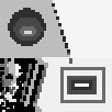
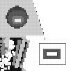
Figure 43: Grey-value example image $f$ (left), its reconstruction $\rho(f)$ (centre) and its reconstruction $\delta(f)$ (right). We can clearly notice, that $f\leq\rho(f)\leq\delta(f)$. In this figure, we have used non-flat SEs $k_{2}$ and $c_{2}$ as described in 42.

We have shown that $(\dot{\sigma},\sigma)$ is an adjunction. By Proposition 2.6 of r4 we have the following lemma.

Lemma 4.2.

Let $f:F(\subseteq\mathbb{\mathchar 69\relax}^{N})\rightarrow L$ be any image. Then, $f$ $\leq\rho(f)$ $=\dot{\sigma}(\sigma(f))$ $=(f\oplus k)|_{S}\bullet k$.

Now, we give the relation between operating after max-pooling and max-pooling after performing the morphological operation, when $\sigma(.)$ and $\rho(.)$ is used for max-pooling and reconstruction, respectively. Let us reiterate. Both the filter $k:K\rightarrow L$ used in max-pooling and reconstruction operators and $c:C(\subseteq S)\rightarrow L$ are not restricted to be flat. Therefore $k$, $K$ and $S$ must only satisfy the conditions of Grey-value Morphological Sampling Theorem 2.14, and $c$ can be any arbitrary non-negative function defined on in the sampled domain, i.e. $C=C\cap S$ and $c=c|_{S}$. Some minor results utilized in the proof of the following proposition are given in the Appendix, Section A.

Figure 44: $\sigma(f\oplus c_{2})$

Figure 45: $\sigma(f)\oplus c_{2}$

Figure 46: $\sigma(f\ominus c_{2})$

Figure 47: $\sigma(f)\ominus c_{2}$

Figure 48: $\sigma((f\oplus k_{2})\ominus c_{2})$

Figure 49: $\sigma(f\circ c_{2})$

Figure 50: $\sigma(f)\circ c_{2}$

Figure 51: $\sigma((f\oplus k_{2})\circ c_{2})$

Figure 52: $\sigma(f\bullet c_{2})$

Figure 53: $\sigma(f)\bullet c_{2}$

Figure 54: $\sigma((f\oplus k_{2})\bullet c_{2})$

Figure 55: $\rho(f)\oplus c_{2}$

Figure 56: $\rho(f\oplus c_{2})$

Figure 57: $\rho(f\ominus c_{2})$

Figure 58: $\rho((f\oplus k_{2})\ominus c_{2})$

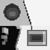
Figure 59: $\rho(f)\circ c_{2}$

Figure 60: $\rho((f\oplus k_{2})\circ c_{2})$

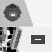
Figure 61: $\rho(f)\bullet c_{2}$

Figure 62: $\rho((f\oplus k_{2})\bullet c_{2})$

Proposition 4.3.

Let $F\subseteq\mathbb{\mathchar 69\relax}^{N}$ and $f:F\rightarrow L$ be the image. The structuring elements $c:C(\subseteq S)\rightarrow L$, $k:K\rightarrow L$ and sieve $S$ are defined as above. Then,

1. $\sigma(f\oplus c)$ $=\sigma(f)\oplus c$,
   i.e. $((f\oplus c)\oplus k)|_{S}$ $=(f\oplus k)|_{S}\oplus c$

2. $\sigma(f\ominus c)$ $\leq\sigma(f)\ominus c$ $\sigma((f\oplus k)\ominus c)$,
   i.e. $((f\ominus c)\oplus k)|_{S}$ $\leq(f\oplus k)|_{S}\ominus c$ $\leq(((f\oplus k)\ominus c)\oplus k)|_{S}$

3. $\sigma(f\circ c)$ $\leq\sigma(f)\circ c$ $\leq\sigma((f\oplus k)\circ c)$,
   i.e. $((f\circ c)\oplus k)|_{S}$ $\leq(f\oplus k)|_{S}\circ c$ $\leq(((f\oplus k)\circ c)\oplus k)|_{S}$

4. $\sigma(f\bullet c)$ $\leq\sigma(f)\bullet c$ $\leq\sigma((f\oplus k)\bullet c)$,
   i.e. $((f\bullet c)\oplus k)|_{S}$ $\leq(f\oplus k)|_{S}\bullet c$ $\leq(((f\oplus k)\bullet c)\oplus k)|_{S}$

5. $\rho(f)\oplus c$ $\leq\rho(f\oplus c)$,
   i.e. $((f\oplus k)|_{S}\bullet k)\oplus c$ $\leq((f\oplus c)\oplus k)|_{S}\bullet k$

6. $\rho(f\ominus c)$ $\leq\rho(f)\ominus c$ $\leq\rho((f\oplus k)\ominus c)$,
   i.e. $((f\ominus c)\oplus k)|_{S}$ $\leq((f\oplus k)|_{S}\bullet k)\ominus c$ $\leq(((f\oplus k)\ominus c)\oplus k)|_{S}\bullet k$

7. $\rho(f)\circ c$ $\leq\rho((f\oplus k)\circ c)$,
   i.e. $((f\oplus k)|_{S}\bullet k)\circ c$ $\leq(((f\oplus k)\circ c)\oplus k)|_{S}\bullet k$

8. $\rho(f)\bullet c$ $\leq\rho((f\oplus k)\bullet c)$,
   i.e. $((f\oplus k)|_{S}\bullet k)\bullet c$ $\leq(((f\oplus k)\bullet c)\oplus k)|_{S}\bullet k$

Proof: I.

$$((f\oplus c)\oplus k)|_{S} =((f\oplus k)\oplus c)|_{S}\text{, by {Proposition 60} of \cite[cite]{\@@bibref{Authors Phrase1YearPhrase2}{r1}{\@@citephrase{[}}{\@@citephrase{]}}}}$$

$$=((f\oplus k)\oplus c|_{S})|_{S}\text{, because $c=c|_{S}$}$$

$$=(f\oplus k)|_{S}\oplus c|_{S}\text{, by Lemma \ref{thm:lemaa}, {I}}$$

$$=(f\oplus k)|_{S}\oplus c$$

II. We first show $((f\ominus c)\oplus k)|_{S}$ $\leq(f\oplus k)|_{S}\ominus c$.

$$((f\ominus c)\oplus k)|_{S} \leq((f\oplus k)\ominus c)|_{S}\text{, by Lemma \ref{thm:l4}, {II}}$$

$$=((f\oplus k)\ominus c|_{S})|_{S}\text{, $\because$ $c=c|_{S}$}$$

$$=(f\oplus k)|_{S}\ominus c|_{S}\text{, by Lemma \ref{thm:lemaa}, {II}}$$

$$=(f\oplus k)|_{S}\ominus c$$

We now show $(f\oplus k)|_{S}\ominus c$ $\leq(((f\oplus k)\ominus c)\oplus k)|_{S}$.

$$(f\oplus k)|_{S}\ominus c =(f\oplus k)|_{S}\ominus c|_{S}\text{, because $c=c|_{S}$}$$

$$=((f\oplus k)\ominus c|_{S})|_{S}\text{, by Lemma \ref{thm:lemaa}, {II}}$$

$$=((f\oplus k)\ominus c)|_{S}$$

$$\leq(((f\oplus k)\ominus c)\oplus k)|_{S}\text{, by Lemma \ref{thm:l1}}$$

III. We first show $((f\circ c)\oplus k)|_{S}$ $\leq(f\oplus k)|_{S}\circ c$.

$$((f\circ c)\oplus k)|_{S} \leq((f\oplus k)\circ c)|_{S}\text{, by Lemma \ref{thm:l5}, {II}}$$

$$=((f\oplus k)\circ c|_{S})|_{S}\text{, because $c=c|_{S}$}$$

$$=(f\oplus k)|_{S}\circ c|_{S}\text{, by Proposition \ref{thm:pb16a}}$$

$$=(f\oplus k)|_{S}\circ c$$

We now show $(f\oplus k)|_{S}\circ c$ $\leq(((f\oplus k)\circ c)\oplus k)|_{S}$.

$$(f\oplus k)|_{S}\circ c =(f\oplus k)|_{S}\circ c|_{S}\text{, because $c=c|_{S}$}$$

$$=((f\oplus k)\circ c|_{S})|_{S}\text{, by Proposition \ref{thm:pb16a}}$$

$$=((f\oplus k)\circ c)|_{S}$$

$$\leq(((f\oplus k)\circ c)\oplus k)|_{S}\text{, by Lemma \ref{thm:l1}}$$

IV. We first show $((f\bullet c)\oplus k)|_{S}$ $\leq(f\oplus k)|_{S}\bullet c$.

$$((f\bullet c)\oplus k)|_{S} \leq((f\oplus k)\bullet c)|_{S}\text{, by Lemma \ref{thm:l5}, {II}}$$

$$=((f\oplus k)\bullet c|_{S})|_{S}\text{, because $c=c|_{S}$}$$

$$=(f\oplus k)|_{S}\bullet c|_{S}\text{, by Proposition \ref{thm:pb17a}}$$

$$=(f\oplus k)|_{S}\bullet c$$

We now show $(f\oplus k)|_{S}\bullet c$ $\leq(((f\oplus k)\bullet c)\oplus k)|_{S}$.

$$(f\oplus k)|_{S}\bullet c =(f\oplus k)|_{S}\bullet c|_{S}\text{, because $c=c|_{S}$}$$

$$=((f\oplus k)\bullet c|_{S})|_{S}\text{, by Proposition \ref{thm:pb17a}}$$

$$=((f\oplus k)\bullet c)|_{S}$$

$$\leq(((f\oplus k)\bullet c)\oplus k)|_{S}\text{, by Lemma \ref{thm:l1}}$$

V.

$$((f\oplus k)|_{S}\bullet k)\oplus c \leq((f\oplus k)|_{S}\oplus c)\bullet k,$$

by Lemma A.6, II

$$=((f\oplus k)|_{S}\oplus c|_{S})\bullet k,$$

because $$c=c|_{S}$$

$$=((f\oplus k)\oplus c|_{S})|_{S}\bullet k,$$

by Lemma 3.4, I

$$=((f\oplus k)\oplus c)|_{S}\bullet k$$

$$=((f\oplus c)\oplus k)|_{S}\bullet k,$$

by Proposition 60 of r1

VI. We first show $((f\ominus c)\oplus k)|_{S}$ $\leq((f\oplus k)|_{S}\bullet k)\ominus c$.

$$((f\ominus c)\oplus k)|_{S}\bullet k \leq((f\oplus k)\ominus c)|_{S}\bullet k,$$

, by Lemma A.4 II

$$=((f\oplus k)\ominus c|_{S})|_{S}\bullet k,$$

because $$c=c|_{S}$$

$$=((f\oplus k)|_{S}\ominus c|_{S})|\bullet k,$$

by Lemma 3.4, II

$$=((f\oplus k)|_{S}\ominus c)|\bullet k$$

$$\leq((f\oplus k)|_{S}\bullet k)\ominus c,$$

by Lemma A.7

In the remaining parts we apply the result III of Grey-value Morphological Sampling Theorem, 2.14, to $(f\oplus k)$ to obtain

$$(f\oplus k)|_{S}\bullet k\leq(f\oplus k).$$ (Eq1)

We now show $((f\oplus k)|_{S}\bullet k)\ominus c$ $\leq(((f\oplus k)\ominus c)\oplus k)|_{S}\bullet k$.

$$((f\oplus k)|_{S}\bullet k)\ominus c \leq(f\oplus k)\ominus c\text{, by \eqref{eq:1}}$$

$$\leq(((f\oplus k)\ominus c)\oplus k)|_{S}\bullet k,$$

by Lemma 4.2

VII.

$$((f\oplus k)|_{S}\bullet k)\circ c \leq(f\oplus k)\circ c\text{, by \eqref{eq:1}}$$

$$\leq(((f\oplus k)\circ c)\oplus k)|_{S}\bullet k,$$

by Lemma 4.2

VIII.

$$((f\oplus k)|_{S}\bullet k)\bullet c \leq(f\oplus k)\bullet c\text{, by \eqref{eq:1}}$$

$$\leq(((f\oplus k)\bullet c)\oplus k)|_{S}\bullet k,$$

by Lemma 4.2

The results I -IV give relations in sampled domain. The results V-VIII give relations in reconstructed images. The interaction between sampling operator $\sigma(.)$ and morphological operations with non-flat SEs is illustrated in Figures 45-54. Figures 56 to 62 illustrate interaction of reconstruction operation $\rho(.)$ with morphological operations using non-flat SEs. In the following examples we have used the non-flat SEs $k_{2}$ and $c_{2}$ as described in Figure 42.

5 Conclusion

In this paper we have built upon classic works of Haralick and co-authors, and we have shown in detail how to transfer digital sampling theorems concerned with four fundamental morphological operations, namely dilation, erosion, opening and closing, from the binary setting to grey-value images.

Using the above results, we have also extended the work of Heijmans and Toet on max-pooling, morphological sampling and reconstruction to use of non-flat structuring elements.

With this paper we have not only worked on closing a gap in the foundation of mathematical morphology. Our aim is also to address some fundamental theoretical aspects of the pooling operation encountered in machine learning. In our future work we also strive to elaborate more on this aspect.

Appendix A Some Minor Results

In this section, we present some smaller results which are utilized in the discussions of Section 4.

Let $F,\>G,\>C,\>K\subseteq\mathbb{\mathchar 69\relax}^{N}$ and $f:F\rightarrow L$, $g:G\rightarrow L$, $c:C\rightarrow L$ and $k:K\rightarrow L$. Let $S\subseteq\mathbb{\mathchar 69\relax}^{N}$ be the sampling sieve.

Lemma A.1.

Let $0\in K$, $k(0)=0$ and $k(u)\geq 0$ $\forall u\in K$. Then, $f\leq f\oplus k$.

Proof: We first show that if $0\in K$ then $F\subseteq F\oplus K$. Clearly, $x\in F$ and $0\in K$ $\Rightarrow$ $(x+0)\in F\oplus K$. Thus, $x\in F\oplus K$. $\therefore F\subseteq F\oplus K$.
We now show $f\leq f\oplus k$. For all $x\in F$ $\subseteq F\oplus K$, we have $(f\oplus k)(x)$ $=\max_{x-u\in F,\>u\in K}\{f(x-u)+\>k(u)\}$ $\geq f(x-0)+k(0)$ $=f(x)$
$\therefore$ $\forall x\in F$, $f(x)\leq(f\oplus k)(x)$.

Lemma A.2.

If $f\leq g$ then $f|_{S}\leq g|_{S}$.

Proof: We have, $\forall x\in F$ $\subseteq G$, $f(x)\leq g(x)$. That is $\forall s\in F\cap S\subseteq G\cap S$, $f|_{S}(s)\leq g|_{S}(s)$. Therefore, $f|_{S}\leq g|_{S}$.

Lemma A.3.

Let $0\in K$, $k(0)=0$ and $k(u)\geq 0$ $\forall u\in K$. Then, $f\ominus k\leq f$.

Proof: We first show that if $0\in K$ then $F\ominus K\subseteq F$.
Clearly, $x\in F\ominus K$ $\Rightarrow\forall u\in K$, $x+u\in F$.
$0\in K$ $\therefore x+0=x\in F$, which implies $F\ominus K\subseteq F$.
We now show $f\ominus k\leq f$.
For any $x\in F\ominus K$, we have, $(f\ominus k)(x)$ $=\min_{x+u\in F,\>u\in K}\{f(x+u)-k(u)\}$ $\leq f(x+0)-k(0)$ $=f(x)$.

Lemma A.4.

1. $(F\ominus C)\oplus K\subseteq(F\oplus K)\ominus C$

2. $(f\ominus c)\oplus k\leq(f\oplus k)\ominus c$

Proof: I.
Let $x\in(F\ominus C)\oplus K$. Then, $x=u+k$ where $u\in F\ominus C$, $k\in K$.
$u\in F\ominus C$ implies $\forall c_{0}\in C$, $u+c_{0}\in F$.
$\Rightarrow$ $\forall c_{0}\in C$, $(u+k)+c_{0}$ $=(u+c_{0})+k\in F\oplus K$.
Therefore, $x=u+k$ $\in(F\oplus K)\ominus C$.
II.
From Umbra Homomorphism Theorem (Theorem 58 of r1 ), we have $U[(f\ominus c)\oplus k]$ $=U[f\ominus c]\oplus U[k]$ $=(U[f]\ominus U[c])\oplus U[k]$. Similarly, $U[(f\oplus k)\ominus c]=$ $(U[f]\oplus U[k])\ominus U[c]$.
We have $(F\ominus C)\oplus K\subseteq(F\oplus K)\ominus C$. Also, using the logic of Part I of the proof, $(U[f]\ominus U[c])\oplus U[k]\subseteq(U[f]\oplus U[k])\ominus U[c]$.
Therefore, we can conclude, $(f\ominus c)\oplus k\leq(f\oplus k)\ominus c$.

Lemma A.5.

1. $(F\circ C)\oplus K$ $\subseteq(F\oplus K)\circ C$

2. $(f\circ c)\oplus k$ $\leq(f\oplus k)\circ c$

Proof: I.

$$(F\circ C)\oplus K =((F\ominus C)\oplus C)\oplus K$$

$$=((F\ominus C)\oplus K\oplus C\text{, by {Prop.\ 3} of \cite[cite]{\@@bibref{Authors Phrase1YearPhrase2}{r1}{\@@citephrase{[}}{\@@citephrase{]}}}}$$

$$\subseteq((F\oplus K)\ominus C)\oplus C\text{, by Lemma \ref{thm:l4}, {I}}$$

$$=(F\oplus K)\circ C$$

II.

$$(f\circ c)\oplus k =((f\ominus c)\oplus c)\oplus k$$

$$=((f\ominus c)\oplus k)\oplus c\text{, by {Prop.\ 60} of \cite[cite]{\@@bibref{Authors Phrase1YearPhrase2}{r1}{\@@citephrase{[}}{\@@citephrase{]}}}}$$

$$\leq((f\oplus k)\ominus c)\oplus c\text{, by Lemma \ref{thm:l4}, {II}}$$

$$=(f\oplus k)\circ c$$

Lemma A.6.

1. $(F\bullet C)\oplus K$ $\subseteq(F\oplus K)\bullet C$

2. $(f\bullet c)\oplus k$ $\leq(f\oplus k)\bullet c$

Proof: I.

$$(F\bullet C)\oplus K =((F\oplus C)\ominus C)\oplus K$$

$$\subseteq((F\oplus C)\oplus K)\ominus C\text{, by Lemma \ref{thm:l4}, {I}}$$

$$=(F\oplus K)\bullet C$$

II.

$$(f\bullet c)\oplus k =((f\oplus c)\ominus c)\oplus k$$

$$\leq((f\oplus c)\oplus k)\ominus c\text{, by Lemma \ref{thm:l4}, {II}}$$

$$=((f\oplus k)\oplus c)\ominus c\text{, by {Prop.\ 60} of \cite[cite]{\@@bibref{Authors Phrase1YearPhrase2}{r1}{\@@citephrase{[}}{\@@citephrase{]}}}}$$

Lemma A.7.

$(f\ominus c)\bullet k$ $\leq(f\bullet k)\ominus c$

Proof:

$$(f\ominus c)\bullet k =((f\ominus c)\oplus k)\ominus k$$

$$\leq((f\oplus k)\ominus c)\oplus k\text{, by Lemma \ref{thm:l4}, {II}}$$

$$=(f\oplus k)\ominus(c\oplus k)\text{, by {Prop.\ 61} of \cite[cite]{\@@bibref{Authors Phrase1YearPhrase2}{r1}{\@@citephrase{[}}{\@@citephrase{]}}}}$$

$$=(f\oplus k)\ominus(k\oplus c)\text{, by {Prop.\ 59} of \cite[cite]{\@@bibref{Authors Phrase1YearPhrase2}{r1}{\@@citephrase{[}}{\@@citephrase{]}}}}$$

$$=((f\oplus k)\ominus k)\ominus c\text{, by {Prop.\ 61} of \cite[cite]{\@@bibref{Authors Phrase1YearPhrase2}{r1}{\@@citephrase{[}}{\@@citephrase{]}}}}$$

$$=(f\bullet k)\ominus c$$

References

- [1] J. Serra, and P. Soille (Eds.): Mathematical morphology and its applications to image processing. Vol. 2. Springer Science and Business Media, (2012)
- [2] L. Najman, and H. Talbot (Eds.): Mathematical Morphology: From Theory to Applications. Wiley-ISTE, (2010)
- [3] J.B.T.M. Roerdink, ”Mathematical Morphology in Computer Graphics, Scientific Visualization and Visual Exploration”, in Proc. ISMM, LNCS 6671, 367–380, (2011)
- [4] R. M. Haralick, S. R. Sternberg, and X. Zhuang. Image analysis using mathematical morphology. IEEE Trans. Pattern Anal. Mach. Intell., 9(4):532–550, 1987.
- [5] R. M. Haralick, X. Zhuang, C. Lin, and J. S. J. Lee. The digital morphological sampling theorem. IEEE Transactions on Acoustics, Speech, and Signal Processing, 37(12):2067–2090, Dec 1989.
- [6] H. Heijmans and A. Toet. Morphological sampling. CVGIP: Image Under- standing, 54(3):384 – 400, 1991.
- [7] H. Heijmans and C. Ronse. The algebraic basis of mathematical morphology i. dilations and erosions. Computer Vision, Graphics, and Image Processing, 50(3):245 – 295, 1990.
- [8] Shen, Yucong, Xin Zhong, and Frank Y. Shih. ”Deep morphological neural networks.” arXiv preprint arXiv:1909.01532 (2019).
- [9] Franchi, Gianni, Amin Fehri, and Angela Yao. ”Deep morphological networks.” Pattern Recognition 102 (2020): 107246.
- [10] Kirszenberg, Alexandre, Guillaume Tochon, Élodie Puybareau, and Jesus Angulo. ”Going beyond p-convolutions to learn grayscale morphological operators.” In International Conference on Discrete Geometry and Mathematical Morphology, pp. 470-482. Springer, Cham, 2021.
- [11] Hermary, R., Tochon, G., Puybareau, É. et al. Learning Grayscale Mathematical Morphology with Smooth Morphological Layers. J Math Imaging Vis 64, 736–753 (2022).
- [12] C. Ronse, H.J.A.M. Heijmans, The algebraic basis of mathematical morphology: II. Openings and closings, CVGIP: Image Understanding, Volume 54, Issue 1, 1991, Pages 74-97, ISSN 1049-9660.
- [13] C. Ronse. 1990. Why mathematical morphology needs complete lattices. Signal Process. 21, 2 (October 1990), 129-154.
- [14] Henk J.A.M. Heijmans, A note on the umbra transform in grayscale morphology, Pattern Recognition Letters, Volume 14, Issue 11, 1993, Pages 877-881, ISSN 0167-8655,
- [15] Goodfellow,I., Bengio,Y., Courville,A.: Deep Learning. MIT Press (2016).
- [16] Haralick, R., Zhuang, X., Lin, C., Lee, J.S.C.: Binary morphology: working in the sampled domain. In: Proc. CVPR. pp. 780–791. IEEE Computer Society (1988)
- [17] Communication in the presence of noise. Proc. IEEE 86 (2) (1998).
- [18] Zhou,Y., Chellappa,R.: Computation of optical flow using a neural network. In:Proc. IEEE International Conference on Neural Networks. pp. 71-78. IEEE Computer Society (1988)
- [19] Matheron,G.: Random Sets and Integral Geometry. Wiley, NewYork(1975)
- [20] Soille,P.:Morphological Image Analysis. Springer, Berlin(2003)
- [21] Serra, J.: Image Analysis and Mathematical Morphology, vol. 1. Academic Press, London (1982)
- [22] Serra, J.: Image Analysis and Mathematical Morphology, vol. 2. Academic Press, London (1988)
- [23] Sridhar, V., Breuß, M.: Sampling of Non-flat Morphology for Grey Value Images. In: Computer Analysis of Images and Patterns, Springer International Publishing, 2021, LNCS Vol. 13053, pp. 88-97