Vacuum-defect wormholes and a mirror world

Abstract

We have recently discovered a smooth vacuum-wormhole solution of the first-order equations of general relativity. Here, we obtain the corresponding multiple-vacuum-wormhole solution. Assuming that our world is essentially Minkowski spacetime with a large number of these vacuum-defect wormholes inserted, there is then another flat spacetime with opposite spatial orientation, which may be called a “mirror” world. We briefly discuss some phenomenological aspects and point out that there will be no significant vacuum-Cherenkov radiation in our world, so that ultrahigh-energy cosmic rays do not constrain the typical size and separation of the wormhole mouths (different from the constraints obtained for a single Minkowski spacetime with similar defects). Other signatures from a “gas” of vacuum-defect wormholes are mentioned, including a possible time machine.

I Introduction

Traversable wormholes appear to require some form of exotic input: exotic matter Ellis1973 ; Bronnikov1973 ; MorrisThorne1988 ; Visser1996 ; Rubakov2014 ; GaoJafferisWall2017 ; Kundu2022 or, as recently pointed out, an exotic spacetime metric Klinkhamer2023 . Specifically, the new solution is characterized by possessing a particular type of degenerate metric (having a 3-dimensional hypersurface with vanishing determinant) and does not require the presence of exotic matter. Physically, the degenerate hypersurface corresponds to a “spacetime defect,” as discussed in previous papers Klinkhamer2014 ; KlinkhamerSorba2014 ; Klinkhamer2018 . (The origin of such a nonsmooth structure may be with the emergence of spacetime itself, as a kind of crystallization of “spacetime atoms.” An exploratory calculation relies on the IIB-matrix-model formulation IKKT-1997 ; Aoki-etal-review-1999 of nonperturbative superstring theory, where the emerging classical spacetime is encoded in the so-called master field Klinkhamer2021-master ; Klinkhamer2021-regBB ; Klinkhamer2022-corfu .)

An explicit example of this new type of wormhole solution is given by the vacuum-defect-wormhole solution, which does not rely on any form of matter, exotic or not. This vacuum-defect wormhole provides, in fact, a smooth solution of the first-order equations of general relativity Horowitz1991 and a brief summary of this mathematical result will be given later on.

This last vacuum solution corresponds to a single wormhole and the present paper discusses the generalization to multiple-vacuum-wormhole solutions. That construction is straightforward but the interpretation is not.

If we live in a nearly flat world with many vacuum-defect wormholes inserted, then this is only possible if there exists also a mirror world with opposite spatial orientation. The potential existence of a mirror world (or mirror universe) has, of course, been discussed before; a selection of research papers is given in Refs. LeeYang1956 ; KobzarevOkunPomeranchuk1966 ; BlinnikovKhlopov1982 ; SenjanovicWilczekZee1984 ; Linde1988 ; Mohapatra-etal2002 ; Das-etal2011 ; Berezhiani-etal-EPJC-2018 ; Dunsky-etal2023 and two review papers appear in Refs. Okun2007 ; Foot2014 . But the hypothetical mirror world we obtain from our vacuum-defect wormholes is rather different from the mirror worlds discussed in the literature. We present, therefore, some exploratory remarks on the vacuum-defect-wormholes phenomenology, postponing a more detailed treatment to the future. Throughout this paper, we use natural units with $c=1$ and $\hbar=1$, unless stated otherwise.

II Single vacuum-defect wormhole

II.1 Tetrad and connection

Let us give a succinct description of the vacuum-defect-wormhole solution (labeled “vac-def-WH-sol” below), with further details in Ref. Klinkhamer2023 . We will use the differential-form notation of Ref. EguchiGilkeyHanson1980 and collect some basic equations of the first-order formulation of general relativity Schrodinger1950 ; Ferraris-etal-1982 ; Wald1984 ; Burton1998 in Appendix A. Different from the standard second-order formulation of general relativity, the first-order formulation does not require the inverse metric $g^{\mu\nu}(x)$, the metric $g_{\mu\nu}(x)$ [or, equivalently, the tetrad $e^{a}_{\phantom{z}\mu}(x)$] suffices.

The spacetime coordinates are assumed to be given by

$$t \in (-\infty,\,\infty)\,,$$ (1a)

$$\xi \in (-\infty,\,\infty)\,,$$ (1b)

$$\theta \in [0,\,\pi]\,,$$ (1c)

$$\phi \in [0,\,2\pi)\,,$$ (1d)

where $\theta$ and $\phi$ are the standard spherical polar coordinates. The proposed tetrad $e^{a}_{\phantom{z}\mu}(x)$ follows from the following dual basis $e^{a}\equiv e^{a}_{\phantom{z}\mu}\,\text{d}x^{\mu}$ :

$$e^{0}\,\Big{|}_{\text{vac-def-WH-sol}} = \text{d}t\,,$$ (2a)

$$e^{1}\,\Big{|}_{\text{vac-def-WH-sol}} = \frac{\xi}{\sqrt{b^{2}+\xi^{2}}}\;\text{d}\xi\,,$$ (2b)

$$e^{2}\,\Big{|}_{\text{vac-def-WH-sol}} = \sqrt{b^{2}+\xi^{2}}\;\text{d}\theta\,,$$ (2c)

$$e^{3}\,\Big{|}_{\text{vac-def-WH-sol}} = \sqrt{b^{2}+\xi^{2}}\;\sin\theta\;\text{d}\phi\,.$$ (2d)

The proposed connection $\omega^{\phantom{z}a}_{\mu\phantom{z}b}(x)$ has the following nonzero components of the corresponding 1-form:

$$\left\{\omega^{2}_{\phantom{z}1},\,\omega^{3}_{\phantom{z}1},\,\omega^{3}_{\phantom{z}2}\right\}\,\Big{|}_{\text{vac-def-WH-sol}} = \left\{-\omega^{1}_{\phantom{z}2},\,-\omega^{1}_{\phantom{z}3},\,-\omega^{2}_{\phantom{z}3}\right\}\,\Big{|}_{\text{vac-def-WH-sol}}$$ (3)

$$= \left\{\text{d}\theta,\,\sin\theta\;\text{d}\phi,\,\cos\theta\;\text{d}\phi\right\}\,,$$

From this tetrad and connection, we obtain a vanishing curvature 2-form $R^{\,a}_{\,\phantom{z}b}\equiv\text{d}\omega^{\,a}_{\,\phantom{z}b}+\omega^{a}_{\phantom{z}c}\wedge\omega^{c}_{\phantom{z}b}\,$,

$$R^{\,a}_{\phantom{z}b}\,\Big{|}_{\text{vac-def-WH-sol}}=0\,,$$ (4)

which corresponds to Riemann tensor $\mathcal{R}_{\kappa\lambda\mu\nu}(x)=0$ in the standard coordinate formulation (the calligraphic symbol indicates the difference with the curvature 2-form $R^{\,a}_{\,\phantom{z}b}$).

For later reference, the metric $g_{\mu\nu}(x)\equiv e^{a}_{\phantom{z}\mu}(x)\,e^{b}_{\phantom{z}\nu}(x)\,\eta_{ab}$ is given by the following line element:

$$ds^{2}\,\Big{|}_{\text{vac-def-WH-sol}}=-dt^{2}+\frac{\xi^{2}}{b^{2}+\xi^{2}}\;d\xi^{2}+\left(b^{2}+\xi^{2}\right)\,\Big{[}d\theta^{2}+\sin^{2}\theta\,d\phi^{2}\Big{]}\,.$$ (5)

With the metric component $g_{11}(x)=\xi^{2}/(b^{2}+\xi^{2})$, this metric is noninvertible at $\xi=0$.

The tetrad from (2) and the connection from (3) are perfectly smooth at $\xi=0$. They solve the first-order vacuum equations of general relativity, as given by (20a) and (20b) in Appendix A. Alternatively, we can verify that the metric $g_{\mu\nu}(x)$ from (5) solves the second-order vacuum equation of general relativity, $\mathcal{R}_{\mu\nu}(x)=0$, defined at $\xi=0$ by continuous extension from its limit $\xi\to 0$ (see, in particular, Section 3.3.1 of Ref. Guenther2017 ).

II.2 Spatial orientability

As preparation for the construction of multiple wormholes, it will be useful to define already two sets of Cartesian coordinates (one for the “lower” world with $\widetilde{l}<-b$ and the other for the “upper” world with $\widetilde{l}>b$):

$$\left\{\begin{array}[]{c}Z_{+}\\ Y_{+}\\ X_{+}\end{array}\right\} = \widetilde{l}(\xi)\;\left\{\begin{array}[]{l}\phantom{Q}\cos\theta\\ \phantom{Q}\sin\theta\,\sin\phi\\ \phantom{Q}\sin\theta\,\cos\phi\end{array}\right\}\,,\;\;\;\;\text{for}\;\;\widetilde{l}(\xi)\equiv\xi\;\sqrt{1+b^{2}/\xi^{2}}\geq b>0\,,$$ (6g)

$$\left\{\begin{array}[]{c}Z_{-}\\ Y_{-}\\ X_{-}\end{array}\right\} = \widetilde{l}(\xi)\;\left\{\begin{array}[]{l}\phantom{Q}\cos\theta\\ \phantom{Q}\sin\theta\,\sin\phi\\ \phantom{Q}\sin\theta\,\cos\phi\end{array}\right\}\,,\;\;\;\;\text{for}\;\;\widetilde{l}(\xi)\equiv\xi\;\sqrt{1+b^{2}/\xi^{2}}\leq-b<0\,,$$ (6n)

$$\left\{Z_{+},\,Y_{+},\,X_{+}\right\} \stackrel{{\scriptstyle\wedge}}{{=}} \left\{Z_{-},\,Y_{-},\,X_{-}\right\}\,,\hskip 45.5244pt\text{for}\;\;|\,\widetilde{l}(\xi)\,|=b\,.$$ (6o)

The last equation implements the identification of “antipodal” points on the two 2-spheres $S^{\,2}_{\pm}$ with $\widetilde{l}=+b$ or $\widetilde{l}=-b$.

In terms of the $\{t,\,\widetilde{l},\,\theta,\,\phi\}$ coordinates, we have the flat metric

$$ds^{2}=-dt^{2}+d\widetilde{l}^{\;2}+\widetilde{l}^{\;2}\,\Big{[}d\theta^{2}+\sin^{2}\theta\,d\phi^{2}\Big{]}\,.$$ (7)

For an arbitrary fixed time $t$, this corresponds to two flat Euclidian 3-spaces with two open balls of equal radius $b$ excised and “antipodal” identifications on the borders of the balls. Still, these coordinates $\{t,\,\widetilde{l},\,\theta,\,\phi\}$ are only useful outside the wormhole throat ($\widetilde{l}>b$ or $\widetilde{l}<-b$) and not for the whole manifold (including the wormhole throat at $\widetilde{l}=\pm b$) . See further discussion in the first technical remark of Section III B in Ref. Klinkhamer2023 , which contains additional references.

Let us, finally, remark that the vacuum-defect-wormhole solution of the present section is of the inter-universe type, connecting two distinct asymptotically-flat spaces (cf. Fig. 1a of Ref. MorrisThorne1988 and Fig. 1.1 of Ref. Visser1996 or, more schematically, Fig. 1 of Ref. Klinkhamer2023 ), whereas an intra-universe wormhole connects to a single asymptotically-flat space (cf. Fig. 1b of Ref. MorrisThorne1988 and Fig. 1.2 of Ref. Visser1996 ). Our two different 3-spaces have opposite orientations, according to the sign flip in (2b) for positive and negative values of $\xi$ [and the different signs of $\widetilde{l}$ in (6g) and (6n)].

The factor $\xi/(b^{2}+\xi^{2})^{1/2}$ in the tetrad component $e^{1}_{\phantom{z}\mu}(x)$ from (2b) is essential for obtaining a smooth solution. A factor $[\xi^{2}/(b^{2}+\xi^{2})]^{1/2}$ would give, from the no-torsion condition (20a), singular terms $\xi/(\xi^{2})^{1/2}$ in certain connection components $\omega^{\phantom{z}a}_{\mu\phantom{z}b}(x)$. In this way, we see that the change in spatial orientability of the two asymptotically-flat spaces is a direct consequence of having a smooth solution of the first-order field equations of general relativity.

III Multiple vacuum-defect wormholes

III.1 Construction

For the description of the multiple-vacuum-defect-wormhole solution, we need two definitions. First, there is the embedding space $M_{\text{embed}}$, which consists of the union of two copies of Euclidean 3-space $E_{3}^{\,(\pm)}$, one copy being labeled by ‘$+$’ (the “upper” world) and the other by ‘$-$’ (the “lower” world). Each of these 3-spaces has standard Cartesian coordinates, so that we have

$$M_{\text{embed}} = E_{3}^{\,(+)}\cup E_{3}^{\,(-)}$$ (8a)

$$E_{3}^{\,(\pm)} : \left(X_{\pm},\,Y_{\pm},\,Z_{\pm}\right)\;\in\;\mathbb{R}^{3}\,.$$ (8b)

The multiple-vacuum-defect-wormhole solutions only cover part of $M_{\text{embed}}$.

Second, we introduce the following definitions (wormhole label $n\in\{1,\,2,\,3,\,\ldots\,,\,N\}$):

$$\left\{\begin{array}[]{c}Z_{\pm}^{(n)}\\ Y_{\pm}^{(n)}\\ X_{\pm}^{(n)}\end{array}\right\} \equiv \widetilde{l}_{n}\left(\xi_{n}\right)\;\left\{\begin{array}[]{l}\phantom{Q}\cos\theta_{n}\\ \phantom{Q}\sin\theta_{n}\,\sin\phi_{n}\\ \phantom{Q}\sin\theta_{n}\,\cos\phi_{n}\end{array}\right\}\,,$$ (9g)

$$\widetilde{l}_{n}\left(\xi_{n}\right) \equiv \xi_{n}\;\sqrt{1+b_{n}^{2}/\xi_{n}^{2}}\;\in\;(-\infty,\,-b_{n}]\cup[b_{n},\,\infty)\,,$$ (9h)

$$\xi_{n} \in (-\infty,\,\infty)\,,\quad\theta_{n}\;\in\;[0,\,\pi]\,,\quad\phi_{n}\;\in\;[0,\,2\pi)\,,$$ (9i)

where the suffix ‘$+$’ on the left-hand side of (9g) holds for $\xi_{n}\geq 0$ and the suffix ‘$-$’ for $\xi_{n}\leq 0$, with “antipodal” identifications at $\xi_{n}=0$ . Note that we allow for wormholes of different sizes $b_{n}>0$. The typical size of the wormholes will be denoted by $\overline{b}$.

We now give the explicit construction of the $N=2$ multiple-vacuum-defect-wormhole solution, with an obvious generalization to larger values of $N$. For the first wormhole ($n=1$) of the pair, we have the following coordinates in $M_{\text{embed}}$:

$$\left\{\begin{array}[]{c}Z_{\pm}\\ Y_{\pm}\\ X_{\pm}\end{array}\right\}_{N=2} = \left\{\begin{array}[]{c}Z_{\pm}^{(1)}\\ Y_{\pm}^{(1)}\\ X_{\pm}^{(1)}\end{array}\right\}\,,\,\;\;\;\;\;\;\;\;\text{for}\;\;X_{\pm}\leq l_{12}/2\,,$$ (10g)

where the right-hand-side entries are defined in (9) and where $$l_{12}>0 (X_{\pm},\,Y_{\pm},\,Z_{\pm})=\big{(}\widehat{X}_{1},\,\widehat{Y}_{1},\,\widehat{Z}_{1}\big{)}=(0,\,0,\,0) b_{1}$$ will be given shortly. This first wormhole is centered at the spatial origins of both worlds, , and has open balls of equal radius removed from the two flat spaces.

For the second wormhole ($n=2$) of the pair, we only discuss a simple case, namely an equal translation along the $X_{\pm}$ axes in both worlds:

$$\left\{\begin{array}[]{c}Z_{\pm}\\ Y_{\pm}\\ X_{\pm}\end{array}\right\}_{N=2} = \left\{\begin{array}[]{c}Z_{\pm}^{(2)}\\ Y_{\pm}^{(2)}\\ X_{\pm}^{(2)}+l_{12}\end{array}\right\}\,,\,\;\;\;\;\;\;\;\;\text{for}\;\;X_{\pm}\geq l_{12}/2\,,$$ (10n)

with

$$l_{12}\;\Big{|}_{N=2} > b_{1}+b_{2}\,.$$ (10o)

This second wormhole is centered on $(X_{\pm},\,Y_{\pm},\,Z_{\pm})=\big{(}\widehat{X}_{2},\,\widehat{Y}_{2},\,\widehat{Z}_{2}\big{)}=(l_{12},\,0,\,0)$ in both worlds and has open balls of equal radius $b_{2}$ removed from the two flat spaces. A sketch appears in Fig. 2. The two balls in the two copies of $\mathbb{R}^{3}$ do not overlap or touch, provided their separation is large enough, as guaranteed by condition (10o). The $N=2$ solution parameters are thus the wormhole radii $b_{n}$ and the wormhole centers $\big{(}\widehat{X}_{n},\,\widehat{Y}_{n},\,\widehat{Z}_{n}\big{)}$, for $n=1$ and $n=2$.

To get $N\geq 3$ multiple vacuum-defect wormholes, we need to add more single wormholes, appropriately shifted so that their excised balls do not overlap or touch. The typical separation of the wormhole mouths will be denoted by $\overline{l}$ and is defined by the wormhole number density $\overline{n}\equiv 1/\overline{l}^{\,3}$.

III.2 Metric

We can be relatively brief about the (flat) metric of the multiple-vacuum-defect-wormhole solution (labeled “multiple-vac-def-WH-sol” below). In between the wormhole mouths, there is the standard flat metric in either 3-space (marked $\pm$),

$$ds^{2}\,\Big{|}_{\text{multiple-vac-def-WH-sol}}^{\text{(outside\;WH-mouths)}}=-dt^{2}+\left(dX_{\pm}\right)^{2}+\left(dY_{\pm}\right)^{2}+\left(dZ_{\pm}\right)^{2}\,,$$ (11)

for the spatial coordinates (8b) of the embedding space.

For the metric at or near the wormhole mouths, we have essentially the metric (5). Considering, for example, the particular wormhole mouth with label $\overline{n}$, the metric is

$$ds^{2}\,\Big{|}_{\text{multiple-vac-def-WH-sol}}^{\text{(near WH-mouth $\overline{n}$)}}=-dt^{2}+\frac{\xi_{\,\overline{n}}^{2}}{b_{\,\overline{n}}^{2}+\xi_{\,\overline{n}}^{2}}\;d\xi_{\,\overline{n}}^{2}+\left(b_{\,\overline{n}}^{2}+\xi_{\,\overline{n}}^{2}\right)\,\Big{[}d\theta_{\,\overline{n}}^{2}+\sin^{2}\theta_{\,\overline{n}}\,d\phi_{\,\overline{n}}^{2}\Big{]}\,,$$ (12)

with coordinates $\theta_{\,\overline{n}}\in[0,\,\pi]$, $\phi_{\,\overline{n}}\in[0,\,2\pi)$, and $\xi_{\,\overline{n}}\in[-\Delta_{\,\overline{n}},\,\Delta_{\,\overline{n}}]$ for a positive infinitesimal $\Delta_{\,\overline{n}}\,$. The corresponding tetrad is given by (2), but now in terms of the spatial coordinates $\{\xi_{\,\overline{n}},\,\theta_{\,\overline{n}},\,\phi_{\,\overline{n}}\}$. The other $N-1$ wormholes have, near their mouths, tetrads of identical structure, which makes for a consistent spatial orientation of the “upper” world, as well as of the “lower” world.

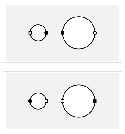
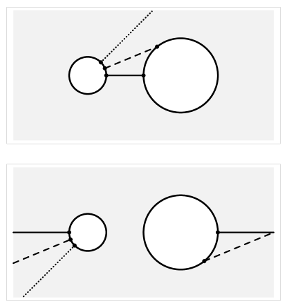
Figure 1: Sketch of the $N=2$ multiple-vacuum-defect-wormhole spacetime, at $Z_{\pm}=0$ and an arbitrary fixed time $t$. The top panel in this figure corresponds to the “upper” world and the bottom panel to the “lower” world. The two worlds are connected by vacuum-defect wormholes. Here, two wormhole throats are shown as heavy circles with “antipodal” spacetime points identified (four distinct spacetime points on the two wormhole mouths are marked by different symbols).

Figure 2: Paths of three light rays in the $N=2$ multiple-vacuum-defect-wormhole spacetime from Fig. 2. The light rays start in the “lower” world on the left and the small dots on the wormhole throats are purely indicative.

IV Phenomenology

IV.1 Preliminary remarks

Let us explore some of the phenomenology from a flat (but nontrivial) spacetime corresponding to a multiple-vacuum-defect-wormhole solution. Physically, we start from an empty spacetime with a “gas” of randomly sprinkled static vacuum-defect wormholes and a small number of material test particles. Some of the details of the construction will become clear as we progress in the present section.

As to cosmology, we are completely agnostic and leave that discussion to a future paper. The problem is that the cosmology of our two-sheeted spacetime requires many further assumptions, for example, if “our” world has a matter-antimatter asymmetry as observed, what about the other world?

IV.2 Light rays

Consider light rays in an empty spacetime with vacuum-defect wormholes, where the flat metric between the wormhole mouths is given by (11). The case of a single wormhole was already discussed in Appendix A of Ref. Klinkhamer2023 . What happens for the case of more wormholes is already clear from the $N=2$ solution.

Figure 2 shows three light rays starting out at the left of the “lower” world and reaching the throat of the left wormhole. For the special light ray along the $N=2$ wormhole-displacement vector (solid curves in Fig. 2), the light ultimately continues towards the right of the “lower” world, after a brief detour in the “upper” world. A similar behavior holds for light rays close to this special ray, except that the returned rays in the “lower” world are parallel shifted (see the in- and outgoing dashed curves in the bottom panel of Fig. 2). But for light rays sufficiently far from the initial special ray, the rays get lost in the “upper” world, as shown by the dotted curves in Fig. 2.

Let us continue the discussion of that last light ray (dotted curves in Fig. 2) for the case of a dense gas of wormholes. The dotted curve in the “upper” world of Fig. 2 will then ultimately hit a wormhole and return to “lower” world. In this way, the propagation of light rays in the “lower” world gets modified by the presence of vacuum-defect wormholes, with a random-walk of parallel shifts (leading to a blurred image of a point source).

IV.3 Dispersion relations

Several years ago, we have calculated BernadotteKlinkhamer2006 the modifications of the photon dispersion relation due to a Swiss-cheese-type spacetime with a “gas” of randomly-positioned static spacetime defects. The results for the modified dispersion relations of photons and Dirac particles are summarized in Appendix B. The calculation outlined in that appendix was for a “gas” of static defect in a single flat spacetime. The question now is what happens in our hypothetical two-sheeted world (as sketched in Figs. 2 and 2).

Recall that, for photons in the single world with localized defects, we are after the solution of the vacuum Maxwell equations in a flat spacetime but with special boundary conditions from the defects (see Fig. 4 in Appendix B). The effects of these boundary conditions are described by fictitious multipoles located inside the holes (this particular construction goes back to Bethe in 1944, who applied it to wave guides). The photon dispersion relation is modified by the fields of these multipoles; see Section II B of Ref. BernadotteKlinkhamer2006 , with further details in Chaps. 3 and 4 of Ref. Bernadotte2006 and Chaps. 12 and 13 of Ref. Schwarz2010 .

But if we now turn to our two-sheeted world and first look at what happens in the lower world, then we see that there are no special boundary conditions on the fields at the wormhole mouths, as shown in the bottom panel of Fig. 2 (whereas there are special boundary conditions on the fields at the defect locations in Fig. 4). Hence, as far as the lower world is concerned, we have the standard plane wave solutions of the Maxwell and Dirac equations with standard dispersion relations.

Still, there are special boundary conditions, but they connect the fields of the lower world to those in the upper world (after a parity transformation, in fact). So, if we have a standard plane wave in the lower world, then we have essentially the same standard plane wave in the upper world but with reversed 3-momentum, $\vec{k}_{U}=-\vec{k}_{L}$. For these unmodified plane waves (labeled “LU-sol”), the dispersion relations of photons ($\gamma$) and structureless Dirac particles ($p$) are simply

$$\left[\omega_{\gamma}^{\text{\,LU-sol}}(k)\right]^{2} \sim c^{2}\,k^{2}+\ldots\,,$$ (13a)

$$[\omega_{p}^{\text{\,LU-sol}}(k)]^{2} \sim c^{2}/\lambda_{p}^{2}+c^{2}\,k^{2}+\ldots\,,$$ (13b)

with $k\equiv|\vec{k}|$ and the reduced Compton wavelength $\lambda_{p}\equiv\hbar/(m_{p}\,c)$ of the spin-${\textstyle\frac{1}{2}}$ particle. The ellipses in the above dispersion relations allow for further terms appearing as corrections to the leading large-wavelength ($k\,\overline{b}\ll 1$) and dilute-gas ($\overline{b}/\overline{l}\ll 1$) approximations.

Anyway, it is clear from (13) that we do not expect significant vacuum-Cherenkov radiation KlinkhamerSchreck2008 , so that ultrahigh-energy cosmic rays (UHECRs) do not constrain the values of the typical wormhole size $\overline{b}$ and the typical wormhole separation $\overline{l}$ (different from the UHECR bounds on defect length scales as reviewed in Appendix B).

IV.4 Scattering

Dispersion relations, modified or not, correspond to essentially stationary phenomena. But we can also use transient phenomena to probe the presence of vacuum-defect wormholes.

Consider a source emitting a light pulse and a distant observer, both located in our (“lower”) world. Then, the wormhole mouths act like perfect absorbers (the light is gone from the lower world). But over a long time the light is returned to the lower world by other wormholes (cf. the solid and dashed curves in Fig. 2 for a single wormhole pair). Averaging over time, the wormhole mouths in the lower world both absorb and emit.

The actual magnitude of scattering effects from the wormhole mouths would be expected to be reduced compared to that of the case of defects, as calculated in Section II C of Ref. BernadotteKlinkhamer2006 , because the wormhole case does not require fictitious dipoles from the boundary conditions. Still, the wormhole boundary conditions will somehow contribute to the scattering. It remains to establish the scattering length $L_{\text{scatt}}$ and its dependence on $\overline{b}$ and $\overline{l}$, possibly with some $k\,\overline{b}$ dependence at smaller wavelengths.

Awaiting the definitive calculation of the scattering length, we can already present a rough estimate. Referring to the discussion in Section II C of Ref. BernadotteKlinkhamer2006 , we take the effective wormhole cross section $\sigma\sim\mathcal{F}\,\pi\,\overline{b}^{\,2}$ [with factor $\mathcal{F}=1$ for a black disk and $\mathcal{F}<1$ from additional emission effects] and the coherence number $N_{\text{coh}}\sim(k\,\overline{l}\,)^{-3}$ for the case considered, $\overline{b}\ll\overline{l}\ll\lambda$. Then the absorption coefficient $\alpha$ (or the inverse of the scattering length $L$) reads

$$\alpha_{\text{scatt}}^{\text{(WH)}}\equiv 1/L_{\text{scatt}}^{\text{(WH)}}\sim\sigma\;\overline{l}^{\,-3}\;N_{\text{coh}}\sim\mathcal{F}\,\pi\,\overline{b}^{\,2}\;k^{-3}\;\overline{l}^{\,-6}\,.$$ (14)

We now demand that $L_{\text{scatt}}^{\text{(WH)}}$ be larger than the source distance $D$.

For some ballpark numbers, we can use the same $2\,\text{TeV}$ gamma-ray flare from Markarian 421 (distance $D\approx 3.8\times 10^{24}\,\text{m}$) as used in Sections IV A and B of Ref. BernadotteKlinkhamer2006 . Demanding $L_{\text{scatt}}^{\text{(WH)}}\gtrsim D/f$ for a factor $f>1$, we get

$$\left(\,\overline{l}/\overline{b}\,\right)^{2}\;\overline{l}^{\,4}\;\Big{|}^{\text{(scatt)}} \gtrsim \pi\,\mathcal{F}\;k^{-3}\;D/f$$ (15)

$$= 1.15\times 10^{-34}\,\text{m}^{4}\;\left(\frac{\mathcal{F}}{1}\right)\,\left(\frac{2.0\,\text{TeV}}{E_{\gamma}}\right)^{3}\,\left(\frac{D}{3.8\times 10^{24}\,\text{m}}\right)\,\left(\frac{10^{2}}{f}\right)\,,$$

where the factor $f$ has been extensively discussed in Section IV B of Ref. BernadotteKlinkhamer2006 and where the actual value of the factor $\mathcal{F}\geq 0$ in the effective wormhole cross section would follow from the definitive calculation.

For a spacetime with single-scale vacuum-defect wormholes ($\overline{b}\sim\overline{l}\,$) and with the assumption $\overline{l}\ll\lambda$, bound (15) for the $\{E_{\gamma},\,D,\,f\}$ values stated gives $\mathcal{F}^{\,1/4}\,10^{-8.5}\,\text{m}\lesssim\overline{l}\ll 10^{-19}\,\text{m}$. Similarly, for Planck-size wormholes ($\,\overline{b}=10^{-35}\,\text{m}$), bound (15) gives $\mathcal{F}^{\,1/6}\,10^{-17.3}\,\text{m}\lesssim\overline{l}\ll 10^{-19}\,\text{m}$. Both examples suggest small values of $\mathcal{F}$. But, as said, these numbers are only indicative.

IV.5 Imaging bound

Following-up on the last remark of Section IV.2, we can use high-resolution imaging by optical microscopes to get bounds on the length-scales of a “gas” of vacuum-defect wormholes (typical size $\overline{b}$ and typical separation $\overline{l}\,$).

For light travelling a distance $L$, there are $N\sim L/\overline{l}$ encounters with the wormhole mouths. As explained in Section IV.2, the built-up parallel shift of the light ray results from a random-walk process and its order of magnitude is given by

$$[\Delta x]_{\text{random-walk}}\sim\sqrt{N}\,\overline{b}\sim\left(\,\overline{b}/\overline{l}\,\right)\;\sqrt{L\,\overline{l}}\,.$$ (16)

In order to get a clear image of an object with substructure $[\delta x]_{\text{object}}$, we must have negligible random-walk parallel shifts of the light ray,

$$[\Delta x]_{\text{random-walk}}\lesssim[\delta x]_{\text{object}}\,.$$ (17)

Putting in some (optimistic) numbers for a high-resolution optical microscope Mertz2019 , we get the following bound on the vacuum-defect-wormhole length scales:

$$\left(\,\overline{b}/\overline{l}\,\right)\,\overline{b}\;\Big{|}^{\text{(opt.\;microscope)}}\lesssim\frac{\left([\delta x]_{\text{object}}\right)^{2}}{L}=4\times 10^{-13}\,\text{m}\;\left(\frac{[\delta x]_{\text{object}}}{200\,\text{nm}}\right)^{2}\,\left(\frac{0.1\,\text{m}}{L}\right)\,,$$ (18)

where the actual $L$ value to be used depends on the details of the instrument. The optical-microscope bound shown in (18) is purely indicative.

Switching over to a transmission electron microscope (TEM, spatial resolution of about $0.1\,\text{nm}=1\,\text{\r{A}}$; see, e.g., Ref. Spence2017 for background and Refs. CreweWallLangmore-1970 ; Chen-etal-2021 for some further images), we have the potential to reduce the upper bound (18) by several orders of magnitude. For a dilute gas of vacuum-defect wormholes, clear TEM images would then give

$$\left(\,\overline{b}/\overline{l}\,\right)\,\overline{b}\;\Big{|}^{\text{(TEM)}}\lesssim 10^{-18}\,\text{m}\;\left(\frac{[\delta x]_{\text{object}}}{1\,\text{\r{A}}}\right)^{2}\,\left(\frac{0.01\,\text{m}}{L}\right)\,,$$ (19)

where (18) has been used with a modest value $L\sim 1\,\text{cm}$ (consistent with lens separations of order $10\,\text{cm}$ as given in Table 2.1 of Ref. Spence2017 ). Ideally, a special-purpose TEM would have condenser lenses designed to produce more or less parallel rays after the rays pass through a 2D sample with subångström structure and to have these parallel rays travelling freely for about $L\sim 10\,\text{cm}$ (possibly broadened by vacuum-defect-wormhole effects) before they enter the rest of the microscope. In that case, the bound (19) could drop to a value of order $10^{-21}\,\text{m}$.

The electron-microscope bound shown in (19) is, for the moment, purely indicative. Still, from (19) for the $[\delta x]_{\text{object}}$ and $L$ values stated, it appears perfectly possible to have a gas of Planck-scale vacuum-defect wormholes, $\,\overline{b}\sim\overline{l}\sim 10^{-35}\,\text{m}$.

Returning to light beams and bound (18), it is perhaps feasible to design an interferometer experiment (with variable arm-lengths and whatever may be needed) to test for random-walk broadening of the beams. Possibly, the LIGO expertise LIGOScientific2007 ; LIGOScientific2014 can be used for obtaining tight constraints on $\left(\,\overline{b}/\overline{l}\,\right)\,\overline{b}$ (optimistically of order $10^{-41}\,\text{m}$, with $[\delta x]_{\text{object}}$ replaced by $[\delta x]_{\text{broadening}}\sim 10^{-19}\,\text{m}$ and $L\sim 1\,\text{km}$).

IV.6 Time machine

It was realized already in the original Morris–Thorne paper MorrisThorne1988 that traversable exotic-matter wormholes appear to allow for backward time travel (a simplified argument was presented in a follow-up paper MorrisThorneYurtsever1988 ). An especially elegant method for getting a time machine was suggested by Frolov and Novikov FrolovNovikov1990 , namely by putting a large mass near one of the mouths of an intra-universe traversable wormhole, so that a clock near that mouth runs slower (gravitational redshift) than a clock near the other mouth. The two clocks are then running at different rates and they will get more and more out of step with each other. A time machine appears when the two clocks are sufficiently far out of step with each other. (The previous two sentences paraphrase two sentences in Section 18.3 of Ref. Visser1996 ; in fact, Sections 18.1 and 18.3 of that reference give a nice discussion of how chronology violation appears to be inescapable if there are traversable wormholes.)

Figure 3: Spacetime-diagram sketches (in rescaled units) of two identical lower-world clocks near two wormhole mouths (corresponding to the heavy dot and the filled square in the bottom panel of Fig. 2). At a lower-world point close to the right wormhole mouth, there can be a static point mass or not (indicated by a star with $M_{\star}>0$ or $M_{\star}=0$). Without a static point mass present (left panel), both clocks run at the same rate: here, the ticks are shown for $t_{\text{left}}=t_{\text{right}}=0,\,1,\,\ldots\,,\,6$. A courageous explorer (with near-light speed) starts out at local time $t_{\text{left}}=5$ from a point near the left wormhole mouth (heavy dot) on a long path in the lower world (full line with arrow in the spacetime diagram of the left panel) to reach a point near the right wormhole mouth (filled square) and then passes quickly through the two wormhole throats (dotted line with arrow in the spacetime diagram of the left panel) back to the starting point (heavy dot) at local time $t_{\text{left}}=6$. With a static point mass present (right panel), the clock on the right runs slower than the clock on the left. Again, an explorer starts out at local time $t_{\text{left}}=5$ from a point near the left wormhole mouth (heavy dot) on a long path in the lower world (full line with arrow in the spacetime diagram of the right panel) to reach a point near the right wormhole mouth (filled square) and then passes quickly through the two wormhole throats (dotted line with arrow in the spacetime diagram of the right panel) back to the starting point (heavy dot) at local time $t_{\text{left}}=3$. The explorer has travelled back in time ($t_{\text{left,\,return}}=3<t_{\text{left,\,start}}=5$) and we have effectively a time machine. The time machine starts working for $t_{\text{left}}\geq 1$ (indeed, the same explorer starting out at local time $t_{\text{left}}=1$ returns at local time $t_{\text{left}}=1$).

It is not difficult to see that we can make a similar time machine by use of multiple vacuum-defect wormholes and a single localized mass. We proceed in two steps.

First, we note that a pair of vacuum-defect wormholes can effectively act as a single intra-universe wormhole. Consider, in fact, a point in the lower world near the heavy dot of the bottom panel in Fig. 2. While staying in the lower world, it is possible to travel along a long path (a large semicircle, for example) to a point near the filled square on the right. Alternatively, it is possible in the lower world to enter the left wormhole at the heavy dot, to emerge in the upper world at the heavy dot, to travel along a straight line in the upper world towards the filled square, to enter the right wormhole at the filled square, and, finally, to re-emerge in the lower world at the filled square. This last route can be very short if the two wormholes of the pair are nearly touching ($l_{12}=b_{1}+b_{2}+\Delta l$ for a positive infinitesimal $\Delta l$, in the notation of Section III.1).

Second, we place a static point mass in the lower world just to the right of the filled square of the bottom panel in Fig. 2. Then, a lower-world clock near the filled square runs slower (gravitational redshift) than a lower-world clock near the heavy dot and a time machine appears after a sufficiently long time (see Fig. 3 with further details in the caption).

Other constructions are certainly possible, but this simple example suffices to show that time machines can, in principle, appear if there exists, at least, one pair of vacuum-defect wormholes and a single point mass which can be freely positioned in one of the worlds. The outstanding question concerns, as emphasized in Ref. FrolovNovikov1990 , the classical and quantum stability of this particular type of time machine.

Still, it is truly remarkable that general relativity in the classical vacuum (in the first-order formalism) appears to allow for backward time travel via the existence of multiple vacuum-defect wormholes. This is all the more surprising as recent results GaoJafferisWall2017 ; Kundu2022 on nonlocal matter quantum effects in a smooth classical spacetime suggest the existence of a traversable wormhole, but without the possibility of getting a time machine. Our time machine (Fig. 3) relies on a nonsmooth spacetime structure, which, as mentioned in Section I, may result from an early phase in the Universe, where spacetime itself (with or without defects) is created IKKT-1997 ; Aoki-etal-review-1999 ; Klinkhamer2021-master ; Klinkhamer2021-regBB ; Klinkhamer2022-corfu .

V Conclusion

If multiple vacuum-defect wormholes are present in our world, then there must exist a mirror world with opposite spatial orientation. The mirror world obtained for vacuum-defect wormholes appears to be quite different from the one discussed in the particle-physics literature LeeYang1956 ; KobzarevOkunPomeranchuk1966 ; BlinnikovKhlopov1982 ; SenjanovicWilczekZee1984 ; Linde1988 ; Mohapatra-etal2002 ; Das-etal2011 ; Berezhiani-etal-EPJC-2018 ; Dunsky-etal2023 ; Okun2007 ; Foot2014 . (Incidentally, our vacuum-defect-wormhole spacetime is also very different from the one discussed in Ref. DokuchaevEroshenko2014 , which considers a nonorientable intra-universe wormhole, even though that wormhole solution is not worked out in detail.) For this reason, we have discussed some of the phenomenology of our hypothetical two-sheeted world.

As mentioned in Section 5 of our original paper Klinkhamer2023 , the typical size $\overline{b}$ of the vacuum-defect wormholes (assuming their relevance to Nature) may be of the order of the Planck length, $l_{P}\equiv(\hbar\,G/c^{3})^{1/2}\sim 10^{-35}\,\text{m}$. In the spirit of the discussion in Section III H of Ref. MorrisThorne1988 , we can imagine that an advanced civilization manages to “harvest” such a very small wormhole and then “fattens” it by adding a finite amount of normal matter (see also Appendix B of Ref. Klinkhamer2023 ).

But the question remains what the initial density of these Planck-scale vacuum-defect wormholes would be. Originally, we thought that the density would be very small, as suggested by tight UHECR bounds on related defects in a single spacetime (as summarized in Appendix B). But the surprising result is that these UHECR bounds do not apply to the vacuum-defect wormholes considered here. Perhaps astrophysics bounds on the typical length scales of the vacuum-defect-wormhole spacetime can be obtained by considering scattering effects. Laboratory bounds can, in principle, be obtained from timing and apparent-brightness measurements of ultrarapid bursts or, similar to the analysis in Sec IV.5, from apparent-size measurements of point-like sources.

Appendix A First-order equations of general relativity in the vacuum

Let us briefly recall the first-order (Palatini) formulation of general relativity, for the case that there is no matter present (an effective classical vacuum). The spacetime fields are then the tetrad $e^{a}_{\mu}(x)$ [building the metric tensor $g_{\mu\nu}(x)\equiv e^{a}_{\phantom{z}\mu}(x)\,e^{b}_{\phantom{z}\nu}(x)\,\eta_{ab}$, with the Minkowski metric $\eta_{ab}$] and the Lorentz connection $\omega^{\phantom{z}a}_{\mu\phantom{z}b}(x)$.

Using differential forms in the notation of Ref. EguchiGilkeyHanson1980 and defining the curvature 2-form $R^{\,a}_{\,\phantom{z}b}\equiv\text{d}\omega^{\,a}_{\,\phantom{z}b}+\omega^{a}_{\phantom{z}c}\wedge\omega^{c}_{\phantom{z}b}$, the first-order vacuum equations of general relativity are Horowitz1991

$$e^{\,[\,a}\wedge D\,e^{\,b\,]} = 0\,,$$ (20a)

$$e^{\,b}\wedge R^{\,cd}\,\epsilon_{abcd} = 0\,,$$ (20b)

with the covariant derivative $D\,e^{b}\equiv\text{d}e^{b}+\omega^{\,b}_{\,\phantom{z}c}\wedge e^{c}$, the completely antisymmetric symbol $\epsilon_{abcd}$, and the square brackets around Lorentz indices denoting antisymmetrization. In terms of $e^{a}_{\mu}$ and $\omega^{\phantom{z}a}_{\mu\phantom{z}b}$, these equations are manifestly first order, as a single exterior derivative d enters $D$ and $R^{\,cd}\,$. Equation (20a) corresponds to the no-torsion condition and (20b) to the Ricci-flatness equation [$\mathcal{R}_{\mu\nu}(x)=0$ in the standard coordinate formulation with the Ricci tensor denoted by a calligraphic symbol, different from the curvature 2-form $R^{\,a}_{\,\phantom{z}b}$ ].

Further discussion of the first-order formulation of general relativity can be found in Refs. Schrodinger1950 ; Ferraris-etal-1982 ; Wald1984 ; Burton1998 .

Appendix B Modified dispersion relations from spacetime defects

The simplest type of static defect considered in Ref. BernadotteKlinkhamer2006 (called “case-1” there) consists of a flat Euclidean 3-space with the interior of a ball of radius $b_{\text{def}}$ removed and antipodal points on the ball’s surface identified. For a single such defect, the topology then corresponds to $\mathbb{R}P^{3}$, the 3-dimensional projective space Klinkhamer2013 . Later, a genuine solution of the Einstein equation, with or without matter, has been found Klinkhamer2014 ; KlinkhamerSorba2014 ; Klinkhamer2013 (see also the subsequent review Klinkhamer2018 with further discussion of the rather surprising phenomenology). But for calculations of the modified dispersion relations only the topology matters.

Let us now consider a “gas” of randomly-positioned case-1 defects (Fig. 4 shows two such defects). Denoting the typical defect size by $\overline{b}_{\text{def}}$ and the typical separation between defects by $\overline{l}_{\text{def}}$, the calculated photon ($\gamma$) dispersion relation in the large-wavelength ($k\,\overline{b}_{\text{def}}\ll 1$) and dilute-gas ($\overline{b}_{\text{def}}/\overline{l}_{\text{def}}\ll 1$) approximations has the following structure (see Eq. (2.14) of Ref. BernadotteKlinkhamer2006 ):

$$\left[\omega_{\gamma}^{\text{defect}}(k)\right]^{2}\sim\left[1-a_{2}\,\big{(}\,\overline{b}_{\text{def}}\big{/}\,\overline{l}_{\text{def}}\big{)}^{3}\right]\,c^{2}\,k^{2}+a_{4}\,\big{(}\,\overline{b}_{\text{def}}\big{/}\,\overline{l}_{\text{def}}\big{)}^{3}\,\overline{b}_{\text{def}}^{\,2}\;c^{2}\,k^{4}+\ldots\,,$$ (21)

with $k\equiv|\vec{k}|$ and positive coefficients $a_{2}=O(10)$ and $a_{4}=O(1)$. (Strictly speaking, the calculation of Ref. BernadotteKlinkhamer2006 was for a dilute gas of identical defects, but the result carries over to the case of having not too different defect sizes.) The calculation in Appendix B of Ref BernadotteKlinkhamer2006 showed that the dispersion relation of a structureless Dirac particle $p$ (for example, an electron or a proton without partons) remains unmodified to lowest order:

$$[\omega_{p}^{\text{defect}}(k)]^{2}\sim c^{2}/\lambda_{p}^{2}+c^{2}\,k^{2}+\ldots\,,$$ (22)

with the reduced Compton wavelength $\lambda_{p}\equiv\hbar/(m_{p}\,c)$ of the particle.

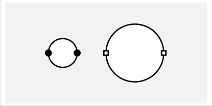
Figure 4: Sketch of the $N=2$ multiple-defect spacetime, at $Z_{\pm}=0$ and an arbitrary fixed time $t$. Each defect corresponds to a 3-sphere with antipodal spacetime points identified. One spacetime point on the left defect is marked by a heavy dot and a different point on the right defect by an open square.

From these results, we see that the photon phase velocity,

$$v_{\text{ph},\,\gamma}\equiv\sqrt{(1-\kappa)/(1+\kappa)}\,c\,,\quad\text{for}\;\;0<\kappa\equiv(a_{2}/2)\,\big{(}\,\overline{b}_{\text{def}}\big{/}\,\overline{l}_{\text{def}}\big{)}^{3}\leq 1\,,$$ (23)

is less than the maximal velocity ($c$) of the Dirac particle, so that there can be Cherenkov radiation, but now already in the vacuum KlinkhamerSchreck2008 . From the observed absence of this type of Lorentz-violating decay processes in ultrahigh-energy cosmic rays (UHECRs), it is possible to obtain stringent bounds KlinkhamerRisse2007 ; KlinkhamerRisse2008 ; KlinkhamerSchreck2008 . A recent bound gives DuenkelNiechciolRisse2023

$$2\,\kappa\;\Big{|}^{\text{(UHECR)}}<6\times 10^{-20}\;(98\%\,\text{CL})\,.$$ (24)

With $2\,\kappa=a_{2}\,\big{(}\,\overline{b}_{\text{def}}\big{/}\,\overline{l}_{\text{def}}\big{)}^{3}$ from (21) and (23) for a Swiss-cheese-type spacetime with static case-1 defects, we obtain

$$\overline{b}_{\text{def}}/\overline{l}_{\text{def}}\;\Big{|}^{\text{(UHECR)}}\lesssim 2\times 10^{-7}\,,$$ (25)

where we have taken $a_{2}=10$ in the $\kappa$ definition. In other words, the defects must correspond to a very dilute gas, with the typical defect separation being more than a million times larger than the typical defect size.

References

- (1) H.G. Ellis, “Ether flow through a drainhole: A particle model in general relativity,” J. Math. Phys. 14, 104 (1973); Errata J. Math. Phys. 15, 520 (1974).
- (2) K.A. Bronnikov, “Scalar-tensor theory and scalar charge,” Acta Phys. Pol. B 4, 251 (1973).
- (3) M.S. Morris and K.S. Thorne, “Wormholes in space-time and their use for interstellar travel: A tool for teaching general relativity,” Am. J. Phys. 56, 395 (1988).
- (4) M. Visser, Lorentzian Wormholes: From Einstein to Hawking (Springer, New York, NY, 1996).
- (5) V.A. Rubakov, “The null energy condition and its violation,” Phys. Usp. 57, 128 (2014), arXiv:1401.4024.
- (6) P. Gao, D.L. Jafferis, and A.C. Wall, “Traversable wormholes via a double trace deformation,” JHEP 12, 151 (2017), arXiv:1608.05687.
- (7) A. Kundu, “Wormholes and holography: An introduction,” Eur. Phys. J. C 82, 447 (2022), arXiv:2110.14958.
- (8) F.R. Klinkhamer, “Defect wormhole: A traversable wormhole without exotic matter,” Acta Phys. Pol. B 54, 5-A3 (2023) arXiv:2301.00724.
- (9) F.R. Klinkhamer, “Skyrmion spacetime defect,” Phys. Rev. D 90, 024007 (2014), arXiv:1402.7048.
- (10) F.R. Klinkhamer and F. Sorba, “Comparison of spacetime defects which are homeomorphic but not diffeomorphic,” J. Math. Phys. 55, 112503 (2014), arXiv:1404.2901.
- (11) F.R. Klinkhamer, “On a soliton-type spacetime defect,” J. Phys. Conf. Ser. 1275, 012012 (2019), arXiv:1811.01078.
- (12) N. Ishibashi, H. Kawai, Y. Kitazawa, and A. Tsuchiya, “A large- reduced model as superstring,” Nucl. Phys. B 498, 467 (1997), arXiv:hep-th/9612115.
- (13) H. Aoki, S. Iso, H. Kawai, Y. Kitazawa, A. Tsuchiya, and T. Tada, “IIB matrix model,” Prog. Theor. Phys. Suppl. 134, 47 (1999), arXiv:hep-th/9908038.
- (14) F.R. Klinkhamer, “IIB matrix model: Emergent spacetime from the master field,” Prog. Theor. Exp. Phys. 2021, 013B04 (2021), arXiv:2007.08485.
- (15) F.R. Klinkhamer, “IIB matrix model and regularized big bang,” Prog. Theor. Exp. Phys. 2021, 063B05 (2021), arXiv:2009.06525.
- (16) F.R. Klinkhamer, “IIB matrix model, bosonic master field, and emergent spacetime,” PoS CORFU2021 259 (2022), arXiv:2203.15779.
- (17) G.T. Horowitz, “Topology change in classical and quantum gravity,” Class. Quant. Grav. 8, 587 (1991).
- (18) T.D. Lee and C.N. Yang, “Question of parity conservation in weak interactions,” Phys. Rev. 104, 254 (1956).
- (19) I.Y. Kobzarev, L.B. Okun, and I.Y. Pomeranchuk, “On the possibility of experimental observation of mirror particles,” Sov. J. Nucl. Phys. 3, 837 (1966).
- (20) S.I. Blinnikov and M.Y. Khlopov, “On possible effects of ‘mirror’ particles,” Sov. J. Nucl. Phys. 36, 472 (1982).
- (21) G. Senjanovic, F. Wilczek, and A. Zee, “Reflections on mirror fermions,” Phys. Lett. B 141, 389 (1984).
- (22) A.D. Linde, “Universe multiplication and the cosmological constant problem,” Phys. Lett. B 200, 272 (1988).
- (23) R.N. Mohapatra, S. Nussinov and V. L. Teplitz, “Mirror matter as selfinteracting dark matter,” Phys. Rev. D 66, 063002 (2002), arXiv:hep-ph/0111381.
- (24) C.R. Das, L.V. Laperashvili, H.B. Nielsen, and A. Tureanu, “Mirror world and superstring-inspired hidden sector of the universe, dark matter and dark energy,” Phys. Rev. D 84, 063510 (2011), arXiv:1101.4558.
- (25) Z. Berezhiani, R. Biondi, P. Geltenbort, I.A. Krasnoshchekova, V.E. Varlamov, A.V. Vassiljev, and O.M. Zherebtsov, “New experimental limits on neutron - mirror neutron oscillations in the presence of mirror magnetic field,” Eur. Phys. J. C 78, 717 (2018), arXiv:1712.05761.
- (26) D.I. Dunsky, L.J. Hall, and K. Harigaya, “A heavy QCD axion and the mirror world,” arXiv:2302.04274.
- (27) L.B. Okun, “Mirror particles and mirror matter: 50 years of speculations and search,” Phys. Usp. 50, 380 (2007), arXiv:hep-ph/0606202.
- (28) R. Foot, “Mirror dark matter: Cosmology, galaxy structure and direct detection,” Int. J. Mod. Phys. A 29, 1430013 (2014), arXiv:1401.3965.
- (29) T. Eguchi, P.B. Gilkey, and A.J. Hanson, “Gravitation, gauge theories and differential geometry,” Phys. Rept. 66, 213 (1980).
- (30) E. Schrödinger, Space-Time Structure (Cambridge UP, Cambridge, UK, 1950).
- (31) M. Ferraris, M. Francaviglia, and C. Reina, “Variational formulation of general relativity from 1915 to 1925 “Palatini’s method” discovered by Einstein in 1925,” Gen. Rel. Grav. 14, 243 (1982).
- (32) R.M. Wald, General Relativity (Chicago UP, Chicago, IL, USA, 1984).
-
(33)
H.S. Burton
“On the Palatini variation and connection theories of gravity,”
PhD Thesis, Waterloo, Ontario, Canada, 1998
[available from https://uwspace.uwaterloo.ca/bitstream/
handle/10012/361/NQ38225.pdf?sequence=1]. -
(34)
M. Guenther,
“Skyrmion spacetime defect, degenerate metric, and negative gravitational mass,”
Master Thesis, Karlsruhe Institute of Technology, September 2017;
[available from
https://www.itp.kit.edu//publications/diploma]. - (35) S. Bernadotte and F.R. Klinkhamer, “Bounds on length-scales of classical spacetime foam models,” Phys. Rev. D 75, 024028 (2007), arXiv:hep-ph/0610216.
-
(36)
S. Bernadotte,
“Einfache Raumzeitschaummodelle und Propagation elektromagnetischer Wellen,”
Diplomarbeit (Master Thesis), Universität Karlsruhe (TH),
August 2006
[available from
https://www.itp.kit.edu//publications/diploma]. - (37) M. Schwarz, “Nontrivial spacetime topology, modified dispersion relations, and an -Skyrme model,” PhD Thesis, Karlsruhe Institute of Technology, July 2010 (Verlag Dr. Hut, Munich, Germany) [ISBN: 978-3-86853-623-2].
- (38) F.R. Klinkhamer and M. Schreck, “New two-sided bound on the isotropic Lorentz-violating parameter of modified-Maxwell theory,” Phys. Rev. D 78, 085026 (2008), arXiv:0809.3217.
- (39) J. Mertz, Introduction to Optical Microscopy, 2nd Edition (Cambridge UP, 2019).
- (40) J.C.H. Spence, High-Resolution Electron Microscopy, 4th Edition (Oxford UP, 2017).
- (41) A.V. Crewe, J. Wall, and J. Langmore, “Visibility of single atoms,” Science 168, 1338 (1970).
- (42) Z. Chen, Y. Jiang, Y. Shao, M.E. Holtz, M. Odstrčil, M. Guizar-Sicairos, I. Hanke, S. Ganschow, D.G. Schlom, and D.A. Muller, “Electron ptychography achieves atomic-resolution limits set by lattice vibrations,” Science 372, 826 (2021), arXiv:2101.00465.
- (43) B.P. Abbott et al. [LIGO Scientific Collaboration], “LIGO: The laser interferometer gravitational-wave observatory,” Rept. Prog. Phys. 72, 076901 (2009), arXiv:0711.3041.
- (44) J. Aasi et al. [LIGO Scientific Collaboration], “Advanced LIGO,” Class. Quant. Grav. 32, 074001 (2015), arXiv:1411.4547.
- (45) M.S. Morris, K.S. Thorne, and U. Yurtsever, “Wormholes, time machines, and the weak energy condition,” Phys. Rev. Lett. 61, 1446 (1988).
- (46) V.P. Frolov and I.D. Novikov, “Physical effects in wormholes and time machines,” Phys. Rev. D 42, 1057 (1990).
- (47) V.I. Dokuchaev and Y.N. Eroshenko, “Nonorientable wormholes as portals to the mirror world,” Phys. Rev. D 90, 024056 (2014), arXiv:1308.0896.
- (48) F.R. Klinkhamer, “A new type of nonsingular black-hole solution in general relativity,” Mod. Phys. Lett. A 29, 1430018 (2014), arXiv:1309.7011.
- (49) F.R. Klinkhamer and M. Risse, “Ultrahigh-energy cosmic-ray bounds on nonbirefringent modified-Maxwell theory,” Phys. Rev. D 77, 016002 (2008), arXiv:0709.2502.
- (50) F.R. Klinkhamer and M. Risse, “Addendum: Ultrahigh-energy cosmic-ray bounds on nonbirefringent modified-Maxwell theory,” Phys. Rev. D 77, 117901 (2008), arXiv:0806.4351.
- (51) F. Duenkel, M. Niechciol, and M. Risse, “New bound on Lorentz violation based on the absence of vacuum Cherenkov radiation in ultrahigh energy air showers,” Phys. Rev. D 107, 083004 (2023), arXiv:2303.05849.