ADA-GP: Accelerating DNN Training By Adaptive Gradient Prediction

Abstract.

Neural network training is inherently sequential where the layers finish the forward propagation in succession, followed by the calculation and back-propagation of gradients (based on a loss function) starting from the last layer. The sequential computations significantly slow down neural network training, especially the deeper ones. Prediction has been successfully used in many areas of computer architecture to speed up sequential processing. Therefore, we propose ADA-GP, which uses gradient prediction adaptively to speed up deep neural network (DNN) training while maintaining accuracy. ADA-GP works by incorporating a small neural network to predict gradients for different layers of a DNN model. ADA-GP uses a novel tensor reorganization method to make it feasible to predict a large number of gradients. ADA-GP alternates between DNN training using backpropagated gradients and DNN training using predicted gradients. ADA-GP adaptively adjusts when and for how long gradient prediction is used to strike a balance between accuracy and performance. Last but not least, we provide a detailed hardware extension in a typical DNN accelerator to realize the speed up potential from gradient prediction. Our extensive experiments with fifteen DNN models show that ADA-GP can achieve an average speed up of $1.47\times$ with similar or even higher accuracy than the baseline models. Moreover, it consumes, on average, 34% less energy due to reduced off-chip memory accesses compared to the baseline accelerator.

1. Introduction

Deep neural networks (DNNs) have shown remarkable success in recent years. They can solve various complex tasks such as recognizing images (Krizhevsky et al., 2012), translating languages (Brown et al., 2020; Vaswani et al., 2017a), driving cars autonomously (Grigorescu et al., 2020), generating images/texts (Qiao et al., 2019), playing games (Silver et al., 2017), etc. DNNs achieve their incredible problem solving ability by training on a vast amount of input data. The de facto standard for DNN training is the backpropagation algorithm (LeCun et al., 2012). This algorithm works by processing input data using the forward pass through the DNN model starting from the first layer to the last. The last layer computes a pre-defined loss function. Then, gradients are calculated based on the loss function and propagated back from the last layer to the first, updating each layer’s weights. Thus, the backpropagation algorithm is inherently sequential: a layer’s weights cannot be updated until all the layers finish the forward pass and gradients are propagated back to that layer.

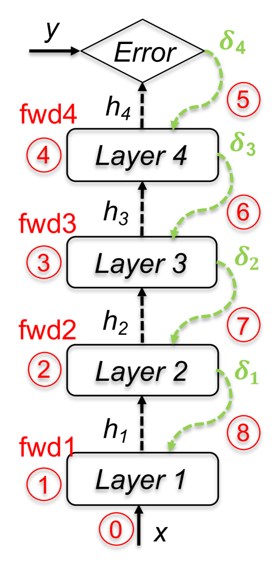
(a) Sequential steps of DNN training algorithm.

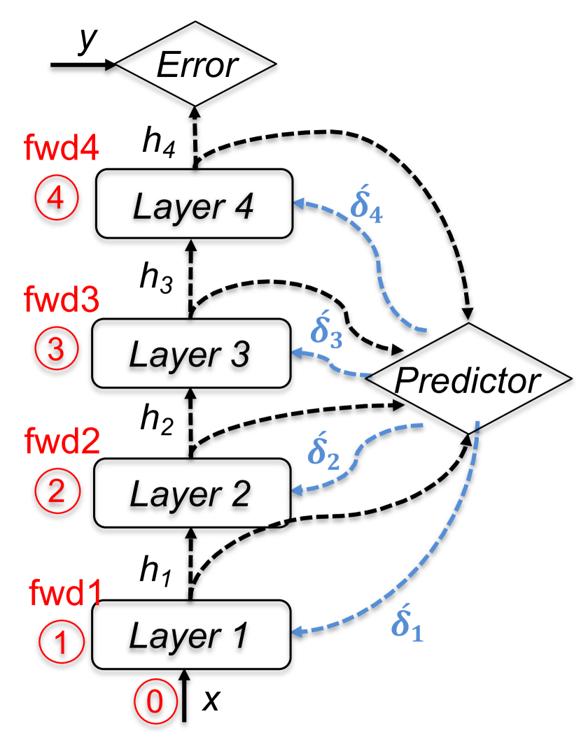
(b) DNN training with gradient prediction.

Figure 1. How gradient prediction speeds up DNN training.

This is shown in Figure 1(a) for an example 4-layer model where the gradients $\delta_{1},...\delta_{4}$ are used to update the weights.

The sequential nature of the backpropagation algorithm makes DNN training a time consuming task. For decades, computer architects have been using prediction to speed up various processing tasks, including sequential ones. For example, predicting branches, memory dependencies, memory access patterns, synchronizations, etc. have been used in various processor architectures to improve performance. Inspired by this line of research, we set out to investigate whether it is possible to use gradient prediction to relax the sequential constraints of DNN training.

There are two major challenges towards gradient prediction.

1. The Curse of Scale: Scalability of gradient prediction arises from two aspects of a DNN model. First, the number of layers of any recent DNN model can be in the range of hundreds; therefore, having one predictor for each layer is not feasible. Second, for many layers, the number of gradients (which should be equal to the number of weights in a given layer) is quite large. In some cases, this number can exceed the number of output activations of a layer. Consequently, predicting a large number of gradients for a layer can be challenging.

2. Accuracy vs. Performance: Always using gradient prediction will speed up DNN training significantly (almost $3x$ speed up by completely eliminating the backpropagation step) but can severely degrade the prediction accuracy. However, if a scheme focuses on predicting high quality gradients and uses them infrequently, it will not affect the prediction accuracy of the DNN model, but reduce the speed up. Therefore, the scheme needs to decide adaptively when and how long to use gradient prediction during DNN training.

To address these challenges, we propose ADA-GP, the first scheme to use gradient prediction for speeding up DNN training while maintaining accuracy. ADA-GP works by incorporating a small neural network model, called a Predictor Model, to predict gradients of various layers of a DNN model. ADA-GP uses a single predictor model for all layers. The model takes the output activations of a layer as inputs and predicts the gradients for that layer (as shown in Figure 1(b)). To predict a large number of gradients, ADA-GP uses tensor reorganization (details in Section 3.6) within a batch of input data. When training starts for a DNN model, the weights of the DNN model are initialized randomly. Therefore, the gradients for the first few training epochs (an epoch is defined as one iteration of DNN training using the entire dataset) are more or less random. Because of this, ADA-GP uses the standard backpropagation algorithm to train the DNN model for a few (e.g., 10) initial epochs. During these epochs, ADA-GP trains the predictor model with the true gradients produced by the backpropagation algorithm. ADA-GP trains the predictor model with each layer’s gradients. After the initial epochs, ADA-GP alternates between DNN training using backpropagated gradients and DNN training using gradients predicted by the predictor model. In other words, for a number of batches (say, $m$), ADA-GP trains the DNN model using the backpropagation algorithm as it is while training the predictor model with true gradients: we call this Phase BP. Then, for the next few batches (say, $k$), ADA-GP switches to DNN training using the predictor model generated gradients: we call this Phase GP. During Phase GP, the backpropagation algorithm is completely skipped, leading to accelerated training of the DNN model. Thus, ADA-GP alternates between Phase BP and Phase GP gradually adjusting the value of $m$ and $k$ to balance accuracy and performance. Finally, we propose some hardware extension in a typical DNN accelerator to implement ADA-GP and realize its full potential.

It should be noted that predicting gradients artificially (as opposed to using backpropagation algorithm) is not new. Several prior works investigate the possibility of utilizing synthetic gradients (Lillicrap et al., 2016; Nøkland, 2016; Xu et al., 2017; Balduzzi et al., 2015; Jaderberg et al., 2017; Czarnecki et al., 2017b, a; Miyato et al., 2017). This line of work is inspired by the biological learning process and produces synthetic gradients using some form of either controlled randomization or per-layer predictors. However, all of the techniques aim at producing better quality gradients for achieving prediction accuracy and convergence rate at least similar to that of the backpropagation algorithm. None of the existing techniques investigate synthetic gradients from the performance improvement point of view. Some techniques (Lillicrap et al., 2016; Nøkland, 2016) require forward propagation of all layers to finish before synthetic gradients can be produced. The majority of the techniques keep the backpropagation computation as it is and require similar or more training time compared to the backpropagation algorithm alone (Jaderberg et al., 2017; Czarnecki et al., 2017a; Miyato et al., 2017). Some of the techniques introduce more trainable parameters into the model, leading to an increased training time (Belilovsky et al., 2020). Last but not least, all of the existing techniques suffer from lower scalability, training stability, and accuracy for deeper models.

1.1. Contributions

We make the following major contributions:

1. ADA-GP is the first work that explores the idea of gradient prediction for improving DNN training time. It does so while maintaining the model’s accuracy.

2. ADA-GP uses a single predictor model to predict gradients for all layers of a DNN model. This reduces the storage and hardware overhead for gradient prediction. Furthermore, ADA-GP uses a novel tensor reorganization technique among a batch of inputs to predict a large number of gradients.

3. ADA-GP uses backpropagated and predicted gradients alternatively to balance performance and accuracy. Moreover, ADA-GP adaptively adjusts when and for how long gradient prediction should be used. Thanks to this novel adaptive algorithm, ADA-GP is able to achieve both high accuracy and performance even for larger DNN models with more sizeable datasets, such as ImageNet.

4. We propose three possible extensions in a typical DNN accelerator with varying degrees of resource requirements to realize the full potential of ADA-GP. Additionally, we show how ADA-GP can be utilized in a multi-chip environment with different parallelization techniques to further improve the performance gain.

5. We implemented ADA-GP in both FPGA and ASIC-style accelerators and experimented with fifteen DNN models using three different datasets - CIFAR10, CIFAR100, and ImageNet. Our results indicate that ADA-GP can achieve an average speed up of $1.47\times$ with similar or even higher accuracy than the baseline models. Also, due to the reduced off-chip memory accesses during the weight updates using predicted gradients, ADA-GP consumes 34% less energy compared to the baseline accelerator.

2. Related Work

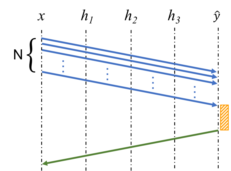
(a) GD

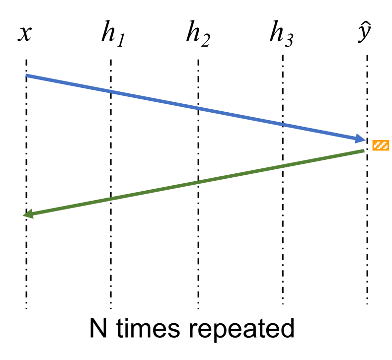
(b) SGD

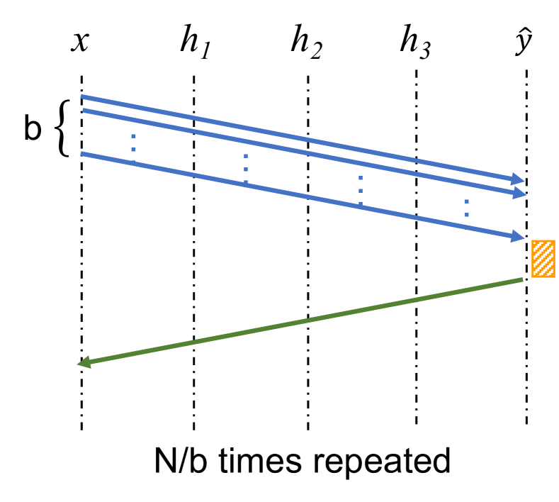
(c) MBGD

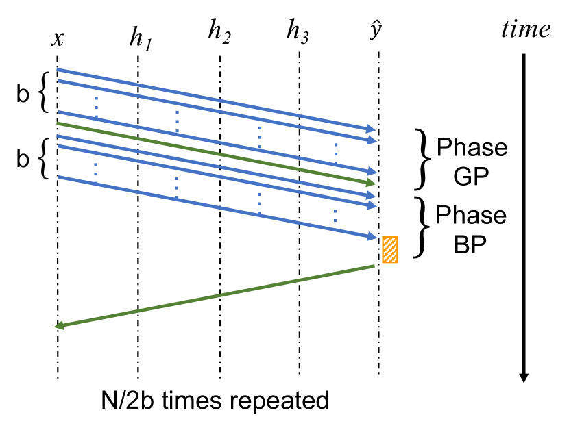
(d) ADA-GP (this work)

Figure 3. Comparison of the learning process and weight updates in (a) Gradient Descent (GD), (b) Stochastic GD (SGD), (c) Mini-batch GD (MBGD), and (d) ADA-GP. An arrow represent the direction of computations through different layers of the network. Here, the network has four layers including three hidden layers; $N$ is the size of input dataset and $b$ is the batch size. Loss calculation is shown as proportional to the computation amount.

Training of a neural network is done using many input-label pairs such as $(x,y)$ with $x$ and $y$ being the input and the corresponding desired label. In the forward pass, the prediction $\hat{y}$ is calculated, whereas the backward pass calculates the prediction error (i.e., loss) at the output layer and propagates it back through the earlier layers to calculate the weight gradients relative to the loss. The weight gradients are used to update the weights of the network. In case of the Gradient Descent (GD) algorithm, all inputs of the training dataset are used to calculate a single loss and perform a single iteration of weight update. Therefore, for larger datasets, GD becomes painstakingly slow. An alternative is Stochastic GD (SGD) where a single input is randomly chosen from the entire dataset to calculate the loss and perform a single iteration of weight update. For larger datasets, SGD is faster but suffers from lower prediction accuracy. A commonly used middle ground is called Mini-batch GD (MBGD) where a batch of random inputs from the dataset is used to calculate the loss and perform a single iteration of weight update. Whether it is GD, SGD, or MBGD, weight update is always dependent on loss calculation which is dependent on processing the input through the forward pass. The only difference among these approaches is the number of inputs that need to be processed. ADA-GP is fundamentally different from these approaches because (in Phase GP) it allows weight updates to be done in parallel with the froward pass without requiring any loss. This is shown in Figure 3.

Jaderberg et al. (Jaderberg et al., 2017) proposed Decoupled Neural Interface (DNI) where a layer receives synthetic gradients from an auxiliary model after output activations of the layer are calculated. The predicted gradients can be used to update the weights of the layer. The auxiliary model is trained based on the backpropagated gradients and the predicted gradients. In other words, DNI requires the backpropagation algorithm to proceed as usual. When a layer has the backpropagated gradients available, these gradients are compared against the predicted gradients, and the auxiliary model is updated. Thus, DNI does not eliminate the backpropagation step at all. Instead, it increases computations of the backpropagation step by including the auxiliary model update as part of the backpropagation step. That is why, DNI does not improve training time. In fact, it slows down the training time. This is different from ADA-GP, where the backpropagation step is adaptively skipped as the DNN training proceeds. Speed up of ADA-GP comes from skipping the backpropagation step altogether. Moreover, the DNI approach was shown to work only for small networks (up to 6 layers) and small datasets such as MNIST. Czarnecki et al. (Czarnecki et al., 2017a) explored the benefits of including derivatives in the learning process of the auxiliary model. The proposed method, called Sobolev Training (ST), considers both the second-order derivatives as well as the backpropagated gradients to train the auxiliary model. The intuition is that by including the derivatives, the auxiliary model will produce higher-quality gradients compared to the DNI approach. However, similar to DNI, it does not eliminate the backpropagation step. Rather, ST increases the backpropagation computations even more by including the computations of the second-order derivatives. Therefore, ST slows down DNN training even further. Miyato et al. (Miyato et al., 2017) proposed a virtual forward-backward network (VFBN) to simulate the actual sub-network above a DNN layer to generate gradients with respect to the weights of that layer. Thus, VFBN does not eliminate backpropagation at all. Instead, it introduces the backpropagation of a different network, namely VFBN. Using this approach, the authors showed comparative accuracy similar to the baseline model with backpropagation-based learning. However, similar to prior approaches, VFBN does not reduce DNN training time.

There is a number of work that uses some form of random or direct gradients from the last layer. Achieving biological plausibility serves as a key motivation for these techniques (Lillicrap et al., 2016; Nøkland, 2016; Xu et al., 2017; Balduzzi et al., 2015), which target the removal of weight symmetry and potential gradient propagation in the backward pass. By substituting symmetrical weights with random ones, Feedback Alignment (FA) (Lillicrap et al., 2016) achieves weight symmetry elimination. Direct FA (Nøkland, 2016) replaces the backpropagation algorithm with random projection, possibly enabling concurrent updates of all layers. The study by Balduzzi et al. (Balduzzi et al., 2015) disrupts local dependencies across consecutive layers, allowing direct error information reception by all hidden layers from the output layer. All of these approaches end up using poor-quality gradients. Consequently, they degrade the prediction accuracy of the DNN model significantly (especially for deeper models) and eventually, end up taking more time to reach the target accuracy. Decoupled Greedy Learning (Belilovsky et al., 2020), Decoupled Parallel Backpropagation (DDG) (Huo et al., 2018b), and Fully Decoupled Training scheme (FDG) (Zhuang et al., 2021) are other strategies that aim to address sequential dependencies of DNN training. While DDG and FDG have been shown to reduce total computation time, they incur large memory overhead due to the storage of a large number of intermediate results. Moreover, they also suffer from weight staleness. Feature Replay (FR)  (Huo et al., 2018a) similarly breaks backward dependency by recomputation. Its performance has been shown to surpass that of backpropagation in various deep architectures. However, FR has a greater computation demand, leading to a slower training time compared to DDG. Finally, these works require all layers to finish the forward propagation first before the weights can be updated. This is different from ADA-GP where weights of a layer can be updated as soon as the output activations are calculated. ADA-GP does not need to wait for the forward propagation of all layers to finish.

There are a number of parallelization strategies for DNN training. Data Parallelism  (Goyal et al., 2017; Li et al., 2020; Sergeev and Del Balso, 2018; You et al., 2018) is a widespread method for scaling up the training processes on parallel machines. However, this method encounters efficiency challenges due to gradient synchronization and model size. Operator Parallelism offers a solution for training larger models by dividing layer operators among multiple workers but faces higher communication requirements. Hybrid techniques  (Jia et al., 2019; Krizhevsky, 2014) combining operator and data parallelism also encounter similar issues. Pipeline Parallelism  (Huang et al., 2019; Fan et al., 2021; Li and Hoefler, 2021; Jain et al., 2020) has been extensively explored to reduce communication volume by partitioning the model in layers, assigning workers to pipeline the layers, and processing micro-batches sequentially. However, ADA-GP is orthogonal to this line of work and can be applied in conjunction with any of these approaches.

3. Adaptive Gradient Prediction

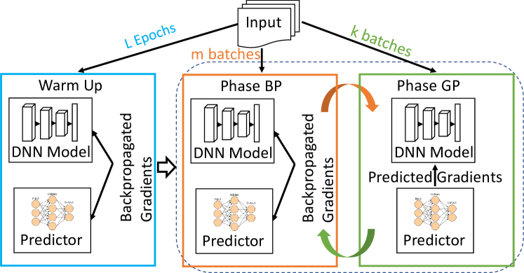
Figure 4. Overview of how ADA-GP uses gradient prediction for DNN training.

3.1. Overview

ADA-GP works in three phases. When DNN training starts, the DNN model is initialized and trained using the standard backpropagation algorithm. During the first few epochs (e.g., $L$ epochs), the predictor model is trained with the true (backpropagated) gradients without using any of the predicted gradients in model training. This is the Warm Up phase (this is reminiscent of the warm up step used in the micro-architectural simulation). Keep in mind that an epoch is one iteration of DNN training with the entire input dataset. Afterward, ADA-GP alternates between the backpropagation (Phase BP) and gradient prediction (Phase GP) phases within an epoch. In Phase BP, the DNN model as well as the predictor model are trained with the backpropagated gradients. This is similar to the Warm Up phase except it lasts for a few (say, $m$) batches of input data during an epoch. Then, ADA-GP starts using the predicted gradients from the predictor model while skipping the backpropagation step altogether. The skipping of backpropagation leads to an accelerated training in Phase GP. Phase GP lasts for a few (say, $k$) batches of input data. After that, ADA-GP operates in Phase BP followed by Phase GP mode. This continues with the value of $m$ and $k$ adapting over time as the DNN training progresses. Thus, ADA-GP alternates between learning the actual gradients (from backpropagation) and applying the predicted gradients (after learning).

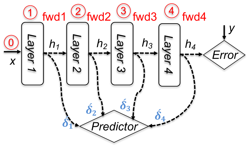
(a) Forward propagation of ADA-GP in Phase BP.

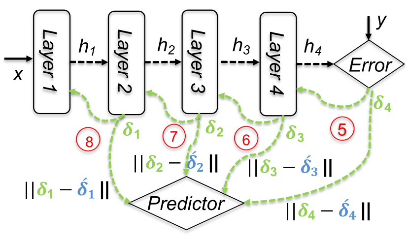
(b) Backpropagation of ADA-GP in Phase BP.

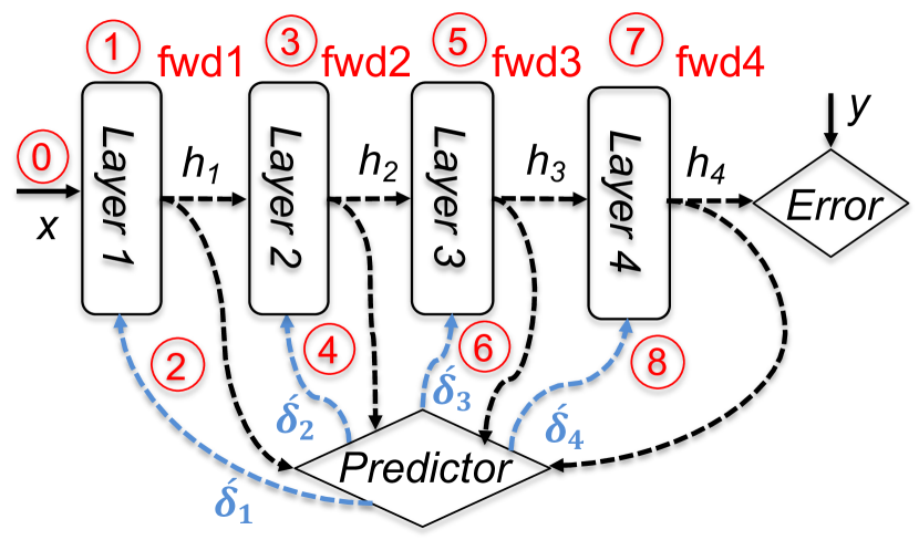
(c) Overall training of ADA-GP in Phase GP.

Figure 5. The structure of ADA-GP in a) forward propagation of Phase BP, b) backward propagation of Phase BP, and c) comprehensive processes within Phase GP that train the initial model using the predicted gradients by predictor model.

3.2. Warm Up of ADA-GP

The intuition behind the Warm Up phase is to initialize the predictor model and ramp up its gradient prediction ability. Since the DNN model is initialized randomly, the backpropagated gradients are more or less random for the initial few epochs. The predictor model learns from the backpropagated gradients of each layer. As a result, the predicted gradients are even worse in quality during these epochs. Because of this, ADA-GP does not apply the predicted gradients to update the DNN model. Instead, the backpropagated gradients are used for that purpose. Presumably, after few epochs, say $L$, the predictor starts to produce gradients that are close to the actual backpropagated gradients, at which point ADA-GP enters into Phase BP and GP.

3.3. Phase BP of ADA-GP

In Phase BP, both the original and predictor models are trained based on the true gradients. Contrary to the DNI (Jaderberg et al., 2017) method, which utilizes synthetic gradients for training the original model and true gradients for training the predictor model, Phase BP of ADA-GP calculates the predicted gradients but does not apply them to the original model’s training. Instead, the true gradients are employed for training both the original and predictor models. This technique maintains a high accuracy for both models while retaining the performance of the DNI approach (Jaderberg et al., 2017). Figure 5(a) & 5(b) depict the training approach of Phase BP for a model with 4-layers.

As illustrated in Figure 5(a), unlike the DNI approach, the weights of the layers are not updated during the forward propagation (steps \raisebox{-.9pt} {0}⃝, \raisebox{-.9pt} {1}⃝, \raisebox{-.9pt} {2}⃝, \raisebox{-.9pt} {3}⃝, and \raisebox{-.9pt} {4}⃝) using predicted gradients. Nevertheless, the predicted gradients $\delta_{1}^{\prime}$, $\delta_{2}^{\prime}$, $\delta_{3}^{\prime}$, and $\delta_{4}^{\prime}$ are still calculated with the predictor model based on the output activations in each layer. These predicted gradients are compared against the true gradients (i.e., $\delta_{1}$, $\delta_{2}$, $\delta_{3}$, and $\delta_{4}$) and the predictor model is trained during the backward propagation. Figure 5(b) shows the backpropagation in Phase BP. As shown in Figure 5(b), two operations are performed when calculating the true gradients of each layer (steps \raisebox{-.9pt} {5}⃝, \raisebox{-.9pt} {6}⃝, \raisebox{-.9pt} {7}⃝, and \raisebox{-.9pt} {8}⃝): 1) the layer weights are updated, and 2) the predictor model is trained. As shown in these figures, in Phase BP, the original model undergoes the standard backpropagation step, while the predictor model is trained concurrently.

3.4. Phase GP of ADA-GP

In Phase GP, the standard backpropagation process is skipped, and the original model is trained based on the predicted gradients. Furthermore, the predictor model’s training is skipped in this phase. Figure 5(c) presents the ADA-GP process in Phase GP. It is important to note that Phase GP is applied on a new batch of inputs, following the completion of Phase BP with the previous batch. As shown in Figure 5(c), Phase GP does not have the true gradient calculations, and it uses the predicted gradients to update the original model’s weights. Also, in this phase, ADA-GP does not train the predictor model.

3.5. Adaptivity in ADA-GP

Following the Warm Up phase, ADA-GP transitions to its standard operation and adaptively alternates between the two primary phases - Phase BP and GP. Initially, it proceeds with Phase GP, utilizing the predicted gradients to train the original model. This phase persists for $k$ batches before switching to Phase BP for $m$ batches. At the outset, $m<k$. This means that, at the beginning, ADA-GP uses predicted gradients more than the true gradients. ADA-GP gradually increases the value of $m$ throughout the training process. As training gets closer to the end, the value of $m$ becomes equal to $k$. From this point onward, the number of training batches in Phase BP is equal to that in Phase GP until the end of the training, and ADA-GP no longer modifies $m$. The reasoning behind this approach is that the model is mostly random at the beginning and has a certain threshold regarding gradient accuracy. However, during the later epochs, the gradients’ changes need to be increasingly precise, necessitating higher quality gradients.

For simplicity in our implementation, we performed some experiments to fix the values of $m$ and $k$ and came up with a simple and efficient heuristic. After the Warm Up phase, we set the $k:m$ ratio to $4:1$ (four batches in phase GP and one batch in phase BP) for the next $4$ epochs. Later, we changed the ratio to $3:1$ for another $4$ epochs. Following this pattern, the ratio was then changed to $2:1$, and ultimately settled at $1:1$ for the remainder of the training.

3.6. Tensor Reorganization

Often the predictor may need to predict a large number of gradients. For that purpose, ADA-GP rearranges the output activations of a DNN layer prior to forwarding them to the predictor model. This is done to 1) maintain the predictor model’s compact size, and 2) ensure higher quality for the predicted gradients.

The primary challenge in predicting the gradients of weights for each layer lies in the fact that the number of weights in some layers is significantly large. When a small predictor tries to predict a large number of gradients, it not only produces poor-quality gradients but also increases the training time of the predictor itself. For example, consider the fourth layer of the VGG13 model (Simonyan and Zisserman, 2014) - Conv2d(in_channels=128, out_channels=256, kernel_size=(3,3), stride=1, padding=1). In this layer, the output activation size is (batch_size, 256, 28, 28). Consequently, the number of trainable weight-related parameters that the predictor model should predict is $128\times 256\times 3\times 3$. A simple predictor model with a single fully connected layer would require an input size of $batch\_size\times 256\times 28\times 28$ and an output size of $128\times 256\times 3\times 3$, necessitating substantial memory storage and computational overhead.

To address this issue, we introduce a novel tensor reorganization technique. It is based on the observation that every input sample within a batch contributes to the weight update. Thus, by taking the average of output activations across the batch, we account for the combined effect of all samples. Furthermore, each individual output channel can be thought of as a distinct training sample (within a batch) with respect to the predictor.

Figure 6 shows how tensor reorganization works for a convolution layer Conv2d(in_ch, out_ch, kernel_size=(k,k)). In this figure, the output activation size is (batch_size, out_ch, W, H), where W and H indicate width and height. This is also the input size to the predictor model. First, we calculate the average across the batch to account for the effects of all samples in a batch, resulting in a tensor with size=(out_ch, W, H). Considering that each layer’s filters have unique impacts on the output gradients, we can treat out_ch as the batch size for the predictor model’s input. In our example, we have out_ch filters with a size of $in\_ch\times k\times k$, generating an output with a channel size of out_ch, where each filter is individually convoluted with inputs to create a single output. The reshaped tensor (input) for predictor model becomes (new_batch_size=out_ch, 1, W, H), and the predictor output size becomes (new_batch_size=out_ch,$in\_ch\times k\times k$). To generalize the predictor model for all layers in a large DNN model, we utilize several pooling layers and a small Conv2d layer based on the input size, followed by a single fully connected layer responsible for predicting gradients. Note that the fully connected layer size depends on the largest layer of the DNN model. Therefore, for smaller layers, we simply mask and skip output operations based on the required size.

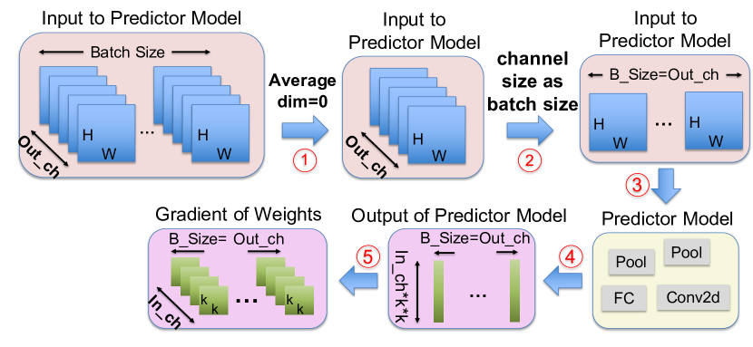
Figure 6. An overview of tensor reorganization for generating gradients of a convolution layer, Conv2d(in_channels=in_ch, out_channels=out_ch, kernel_size=(k,k)). The predicted gradient dimensions should match the weight dimensions (in_ch, out_ch, k, k). predictor model input has the shape of (batch_size, out_ch, W, H).

3.7. Timeline of ADA-GP

Figure 7 illustrates the timeline of the baseline system for a 4-layer neural network model. We assume that the duration of the backward (BW) pass is twice as long as the forward (FW) pass. To simplify the explanation, we focus on the timeline for a single-chip system. We will explore further details about multi-chip pipelining techniques in Section 3.8. As depicted in Figure 7, it is evident that the baseline system requires 12 time steps to complete the operation of a 4-layer model for a single batch. In this figure, the duration of each time step is equivalent to the FW pass time for one layer. Throughout the remainder of this section, we will employ this definition of a $step$ in our explanation.

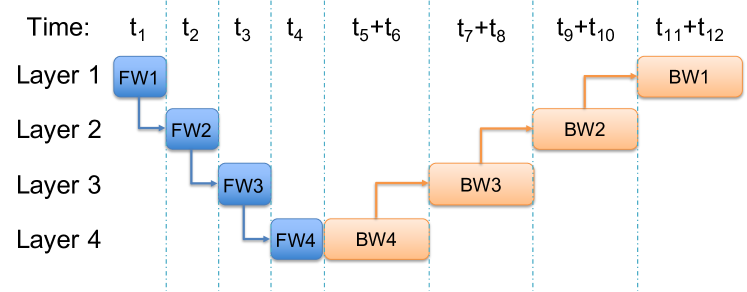
Figure 7. Baseline system timeline for a 4-layer neural network model.

Figure 8 shows the timeline of ADA-GP in Phase BP. As mentioned in Section 3.3, during this phase, ADA-GP trains both the original and predictor models using the true gradients in the BW pass.

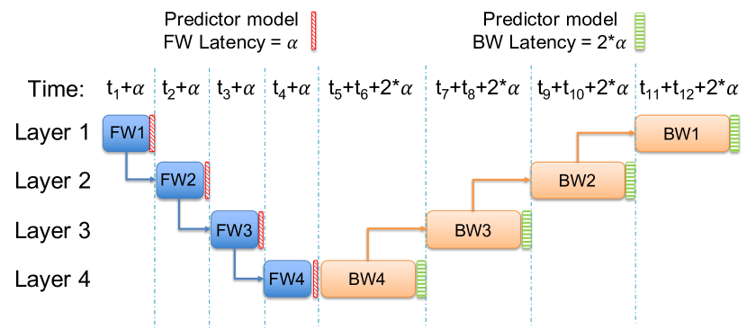
Figure 8. ADA-GP timeline in Phase BP.

As illustrated in Figure 8, there is some latency for the FW pass of the predictor model. This is represented by $\alpha$. This latency is smaller than the FW pass latency of each layer of the original model. Consequently, the latency of the BW pass of the predictor model is set to 2$\alpha$. As demonstrated in this figure, ADA-GP increases the model’s training time by 12$\alpha$. This value is directly linked to the predictor model’s size and the number of operations in its FW and BW pass.

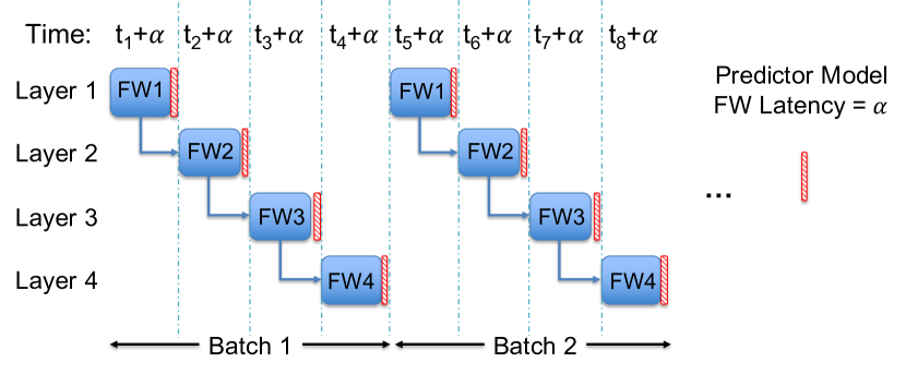
Figure 9. ADA-GP timeline in Phase GP.

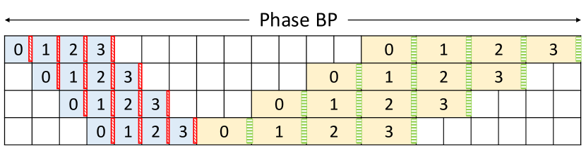
(a) Phase BP

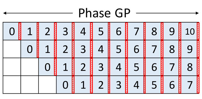
(b) Phase GP

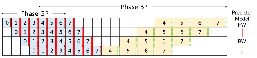
(c) Transition from Phase GP to Phase BP

Figure 10. Structure of ADA-GP over GPipe (Huang et al., 2019) during a) Phase BP, b) Phase GP, c) transition from Phase BP to Phase GP.

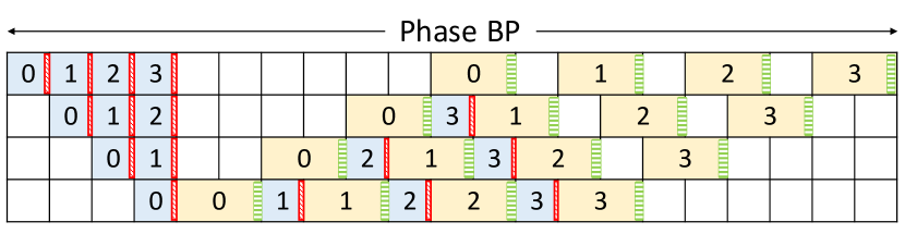
(a) Phase BP

(b) Phase GP

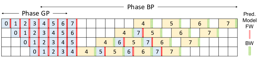
(c) Transition from Phase GP to Phase BP

Figure 11. Structure of ADA-GP over DAPPLE (Fan et al., 2021) during a) Phase BP, b) Phase GP, c) transition from Phase BP to Phase GP.

(a) Phase BP

(b) Phase GP

(c) Transition from Phase GP to Phase BP

Figure 12. Structure of ADA-GP over Chimera (Li and Hoefler, 2021) during a) Phase BP, b) Phase GP, c) transition from Phase BP to Phase GP.

Figure 9 presents the timeline of ADA-GP in Phase GP. As mentioned in Section 3.4, the BW process is skipped in this phase, and the predictor model is not trained. However, the original DNN model is trained using the predicted gradients generated by the predictor model. In Figure 9, it is evident that the BW pass is entirely eliminated, leaving only the FW pass of the original model and a minor delay for the FW pass of the predictor model. Consequently, ADA-GP can minimize the processing time to merely 4+4$\alpha$ steps. As illustrated in Figures 5(a), 5(b), and 5(c), ADA-GP is capable of decreasing the processing time for two epochs from 24 steps in the baseline system to 16+16$\alpha$. As an added benefit of skipping the BW pass in Phase GP, ADA-GP reduces off-chip traffic. Since the weights are updated as the FW pass proceeds, ADA-GP does not need to load the weights and activations from some off-chip memory as is traditionally done in the case of BW pass. This significantly reduces energy consumption. More details are presented in Section 6.6.2.

3.8. ADA-GP in Multi-Device Hardware

A commonly used approach for accelerating DNN training in multiple devices involve pipelining techniques to execute several layers concurrently. ADA-GP is orthogonal to this approach and can be integrated with it. To this end, we examine three prominent pipelining strategies - GPipe(Huang et al., 2019), DAPPLE(Fan et al., 2021), Chimera(Li and Hoefler, 2021) and explain how ADA-GP can be incorporated with them to further speed up the training process. For the ease of explanation, we assume in this section that there are four devices working concurrently, and the batch is divided into four segments, with each device processing one segment at a time.

Figure 10 shows how various ADA-GP phases work when implemented on top of the GPipe approach (Huang et al., 2019). As depicted in Figure 10(a), the ADA-GP operation in Phase BP is similar to the original GPipe method. Note that the duration of each step in ADA-GP differs from that in the original GPipe method. The step size of ADA-GP depends on its implementation as outlined in Section 4.2. Figure 10(b) shows the ADA-GP in Phase GP. In this figure, since ADA-GP eliminates the initial backpropagation process and employs predicted gradients for weight updates, it can initiate the subsequent batch’s process immediately after completing the current batch’s forward propagation. In doing so, ADA-GP can fill all gaps present in the original GPipe method. Lastly, Figure  10(c) illustrates how ADA-GP transitions from Phase BP to Phase GP without causing any additional delay. Another important point that should be taken into consideration is that ADA-GP reduces the number of synchronization steps to half and can save time and energy due to this reduction.

Figure 11 illustrates how various stages of ADA-GP can be integrated with the DAPPLE method (Fan et al., 2021). Like the GPipe strategy, the configuration of ADA-GP in Phase BP closely resembles the original DAPPLE design. The depiction of ADA-GP during Phase GP can be observed in Figure 11(b). As demonstrated in this figure, ADA-GP effectively eliminates the reliance between forward and backward propagation, filling all gaps in the training procedure. Additionally, Figure 11(c) portrays the shift from Phase BP to Phase GP.

The complete structure of the various stages of ADA-GP when implemented alongside the Chimera method (Li and Hoefler, 2021) is depicted in Figure  12. As with earlier strategies, the structure of ADA-GP during Phase BP closely mirrors the initial Chimera design. In Phase GP, it is capable of operating all layers concurrently, eliminating any gaps. Furthermore, a transition between phases incurs no additional delays.

4. Implementation Details

4.1. Baseline DNN Accelerator

Figure 13 illustrates a standard DNN accelerator design, featuring multiple hardware processing elements (PEs). These PEs are interconnected vertically and horizontally via on-chip networks. A global buffer stores input data, weights, and intermediate results. The accelerator is connected to external memory for inputs and outputs. Each PE is equipped with registers for holding inputs, weights, and partial sums, as well as multiplier and adder units. Inputs and weights are distributed across the PEs, which then generate partial sums following a specific dataflow  (Janfaza et al., 2023).

Figure 13. Baseline hardware accelerator.

Various dataflows have been suggested in the literature (Chen et al., 2017, 2016; Kwon et al., 2018; Janfaza et al., 2023) to enhance different aspects of DNN operations, such as Weight-Stationary (WS)  (Sankaradas et al., 2009; Chakradhar et al., 2010; Gokhale et al., 2014), Output-Stationary (OS) (Du et al., 2015), Input-Stationary (IS) (Sze et al., 2017), and Row-Stationary (RS) (Chen et al., 2016). The dataflow’s designation often indicates which data remains constant in the PE during computation. In the Weight-Stationary (WS) approach, each PE retains a weight in its register, with operations utilizing the same weight assigned to the same PE unit (Chen et al., 2017). Inputs are broadcasted to all PEs over time, and partial results are spatially reduced across the PE array after each time step. This method minimizes energy consumption by reusing filter weights and reducing weight reads from DRAM. Output-Stationary (OS) (Peemen et al., 2013) focuses on accumulating partial results within each PE unit. At every time step, both input and filter weight are broadcasted across the PE array, with partial results calculated and stored locally in each PE’s registers. This method minimizes data movement costs by reusing partial results. Input-Stationary (IS) involves loading input data once and keeping it in the registers throughout the computation. Filter weights are unicasted at each time step, while partial results are spatially reduced across the PE array. This strategy reduces the cost of sequentially reading input data from DRAM. Row-Stationary dataflow assigns each PE one row of input data to process. Filter weights stream horizontally, inputs stream diagonally, and partial sums are accumulated vertically. Row-Stationary has been proposed in Eyeriss (Chen et al., 2016) and is considered one of the most efficient dataflows to maximize data reuse.

4.2. ADA-GP Hardware Implementation

The general architecture of the ADA-GP is similar to the baseline accelerator shown in Figure 13. To implement ADA-GP, we propose three designs, striking a balance between hardware resource constraints and the degree of acceleration. Figure 14 shows the three distinct designs we proposed for ADA-GP.

(a) ADA-GP-MAX architecture: This design employs distinct specialized PEs and memory for executing predictor model calculations. This allows for the simultaneous processing of predictor model operations alongside the original model.

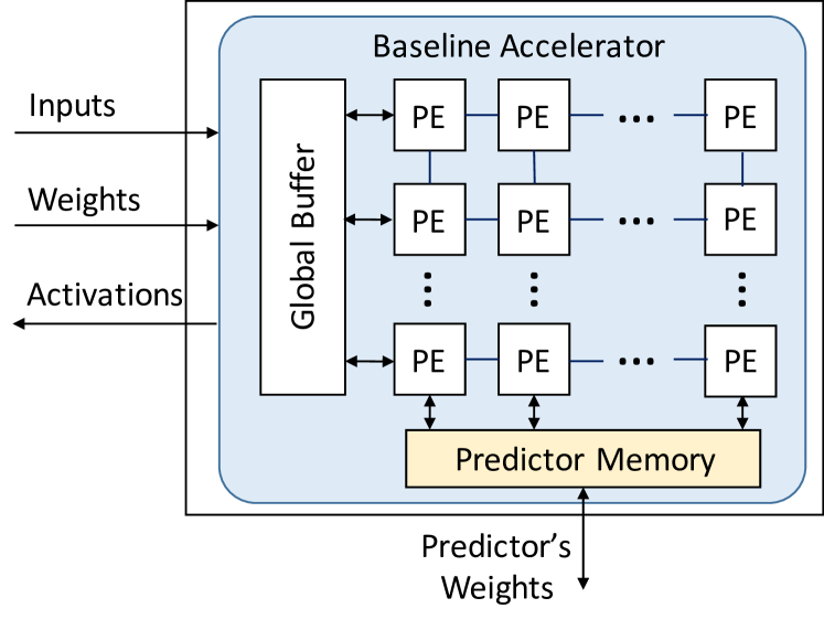
(b) ADA-GP-Efficient architecture: This design does not have a specific PE-Array for predictor model however it has specific memory for saving the predictor’s weights and starts the predictor model computations after finishing the original.

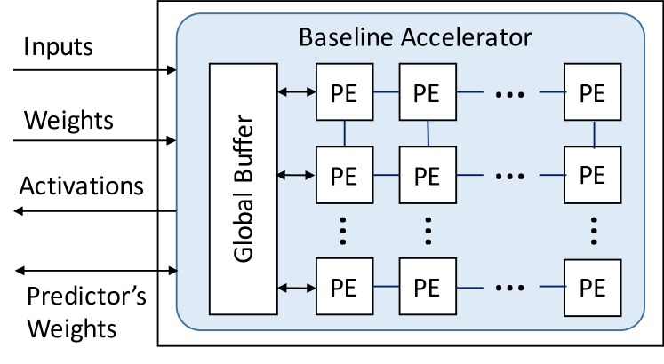
(c) ADA-GP-LOW architecture: This design has no specific hardware overhead for predictor model computations. Upon completion of the original model’s operation, it initiates the predictor model’s functioning by loading the predictor’s weights.

Figure 14. Three distinct ADA-GP approaches, balancing the trade-off between hardware overhead and the degree of acceleration.

Figure 14(a) displays the architecture of ADA-GP-MAX. This configuration incorporates an additional PE Array and memory for predictor model computations and weights storage, respectively. Consequently, ADA-GP can initiate the predictor model’s gradient prediction operations concurrently with the original model’s computations, overlapping the processes and accelerating training. This design offers the most acceleration but also has more hardware overhead in comparison with other designs.

To offset the hardware overhead of ADA-GP-MAX, Figure 14(b) presents the ADA-GP-Efficient architecture. Instead of an extra PE array for the predictor model’s calculations, this design features a separate memory to store predictor model’s weights and commence its operations immediately after completing the original layer computations. While this configuration saves time and energy consumption related to reading and storing predictor’s weights, it must wait for the original model’s operation to finish before starting the predictor model computations.

Aiming to further reduce the hardware overhead of the ADA-GP design, Figure 14(c) depicts the ADA-GP-LOW structure. This layout eliminates all additional hardware overhead from the original design and reuses existing resources for predictor model computations. First, it completes the original model’s operations, then, after saving all necessary changes, loads the predictor’s weights and employs the original PE Array for predictor model computations and updates.

5. Experimental Setup

5.1. ADA-GP Hardware Setup

We implemented ADA-GP hardware in both FPGA and ASIC platforms. For FPGA implementation, we employed the Virtex 7 FPGA board  (Xilinx, 2007), configured through the Xilinx Vivado  (Xilinx, [n. d.]) software. For ASIC implementation, the Synopsys Design Compiler  (Synopsys, [n. d.]) was used, and the design was developed using the Verilog language. Our implementation utilized a weight stationary accelerator with 180 PEs as the baseline. In the FPGA design, the model’s inputs and weights are stored in an external SSD connected to the FPGA. Block memories are employed to load one layer’s weights and inputs while storing the corresponding outputs. Performance, power consumption, hardware utilization, and other hardware-related metrics are gathered from the synthesized and placed and routed FPGA design using Vivado and the synthesized ASIC design using the Design Compiler.

5.2. ADA-GP Software Setup

We gathered various model accuracy results from the PyTorch (Paszke et al., 2019) implementation of ADA-GP. Fifteen networks are considered, including Inception-V4 (Szegedy et al., 2016a), Inception-V3 (Szegedy et al., 2016b), Densenet201 (Huang et al., 2017), Densenet169 (Huang et al., 2017), Densenet161 (Huang et al., 2017), Densenet121 (Huang et al., 2017), ResNet152 (He et al., 2016), ResNet101 (He et al., 2016), ResNet50 (He et al., 2016), VGG19 (Simonyan and Zisserman, 2014), VGG16 (Simonyan and Zisserman, 2014), VGG13 (Simonyan and Zisserman, 2014), MobileNet-V2 (Howard et al., 2018), Transformer (Vaswani et al., 2017b), and YOLO-v3 (Redmon and Farhadi, 2018). Our method is applied to three different datasets: ImageNet (Deng et al., 2009), Cifar100 (Krizhevsky et al., 2009), and Cifar10 (Krizhevsky et al., 2009). For the transformer, we used the Multi30k (Elliott et al., 2016) dataset and reported accuracy and BLEU scores (Papineni et al., 2002) separately in Section 6.4. Also, for the YOLO-v3 (Redmon and Farhadi, 2018) object detection model, we utilized the Pascalvoc (Everingham et al., 2015) Visual Object Classes dataset.

During the training of ADA-GP and the baseline, the initial learning rate was set to 0.001 for the original models and 0.0001 for the predictor model. We employed SGD with Momentum and Adam optimizers for the original and predictor models, respectively. Additionally, we utilized the PyTorch ReduceLROnPlateau scheduler with default parameters for adaptive learning rate updates, while a MultiStepLR scheduler was applied for the predictor model scheduler. Top 1 accuracy was reported for the various models. To evaluate training costs, end-to-end training costs were calculated.

6. Evaluation

Numerous previous studies have explored the potential of employing synthetic gradients in their research  (Lillicrap et al., 2016; Nøkland, 2016; Xu et al., 2017; Balduzzi et al., 2015; Jaderberg et al., 2017; Czarnecki et al., 2017b, a; Miyato et al., 2017). These approaches generate synthetic gradients through controlled randomization or per-layer predictors. However, none of these methods focus on performance enhancement or skipping the backpropagation step. Moreover, their accuracy is less than or equal to that of backpropagation-based training. Therefore, at best, those approaches will have accuracy and performance similar to the backpropagation-based training. This is why we use the backpropagation technique as our baseline to compare both the accuracy and performance of ADA-GP.

6.1. Accuracy Analysis

6.1.1. Model Accuracy

We evaluate the accuracy of the proposed method across thirteen different deep-learning models using three distinct datasets: ImageNet, Cifar100, and Cifar10, and compare it with the baseline Backpropagation (BP) approach.

Table 1. Accuracy comparison between ADA-GP and Baseline (BP) for CIFAR10, CIFAR100 & ImageNet dataset.

	CIFAR10		CIFAR100		ImageNet
	BP	ADA-GP	BP	ADA-GP	BP	ADA-GP
ResNet50	92.97	93.76	75.44	75.73	74.73	73.97
ResNet101	92.78	93.62	73.23	75.38	76.26	75.71
ResNet152	92.8	93.12	72.01	73.7	76.68	76.23
Inception-V4	91.22	91.35	70.52	72.42	76.23	75.9
Inception-V3	93.04	93.88	76.41	77.68	74.44	73.87
VGG13	91.52	92.55	70.48	70.41	70.68	70.68
VGG16	91.32	92.34	70.36	70.47	72.07	71.98
VGG19	91.18	92.51	69.69	69.85	72.94	72.83
DenseNet121	93.2	93.63	76.25	76.12	75.25	74.51
DenseNet161	93.48	94.19	76.87	77.38	76.43	76.71
DenseNet169	93.24	94.15	75.57	76.4	75.36	75.3
DenseNet201	93.26	94.13	76.37	76.96	75.52	75.56
MobileNet	90.08	91.34	68.11	68.47	69.88	69.23

Table 1 presents the accuracy comparison between the proposed ADA-GP and the baseline BP for the Cifar10, Cifar100, and ImageNet datasets. As shown in this table, in the Cifar10 dataset, ADA-GP effectively boosted the accuracy of all models by as much as 1.45% and an average of 0.75%. When applied to the Cifar100 dataset, ADA-GP similarly yielded improvements, with accuracy enhancements of up to 2.15% and an average gain of 0.88%. To further verify the efficacy of our approach, we applied ADA-GP on the ImageNet dataset. The final two columns of Table 1 reveal that ADA-GP preserved the accuracy of all models at levels nearly equivalent to the baseline (BP), with a negligible average reduction of 0.3%. In certain cases, such as with DenseNet161 and DenseNet201 our proposed method even increased accuracy by 0.28% and 0.04% respectively, and in VGG13, the accuracy remained unchanged.

6.1.2. Predictor Accuracy

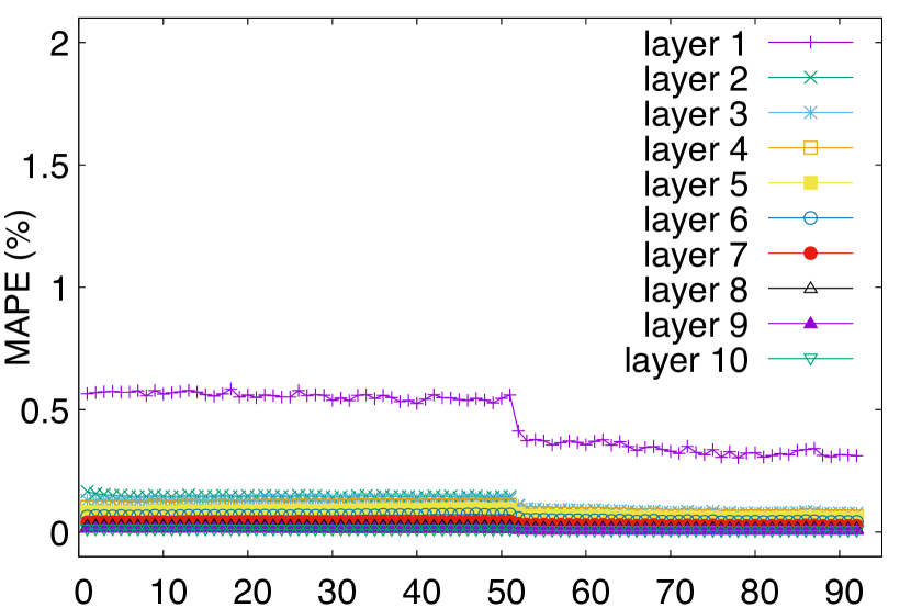
(a) MAPE

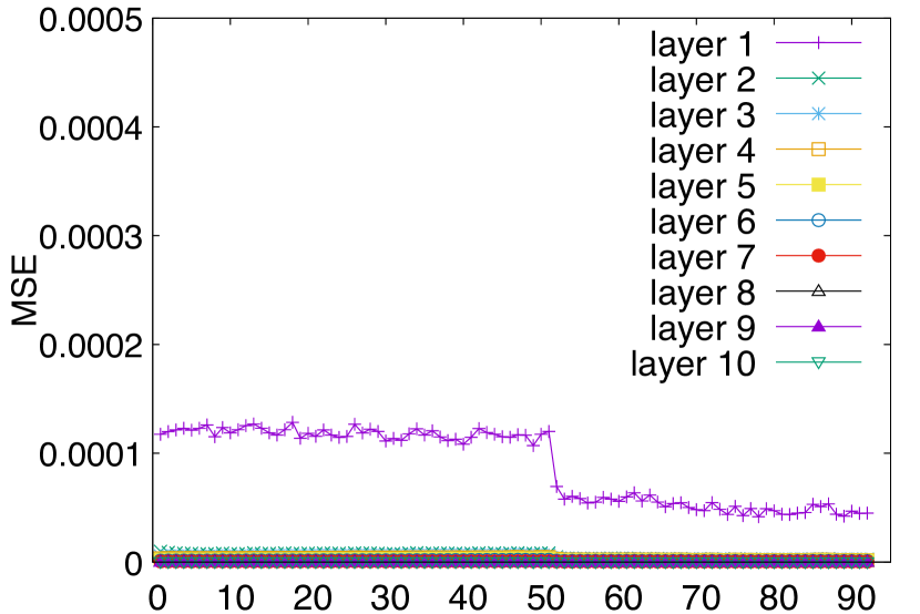
(b) MSE

Figure 15. MAPE and MSE of the predictor model in different layers of VGG13 during the training.

We use the Mean Absolute Percentage Error (MAPE) to show the accuracy and performance of the predictor model  (wikipedia, [n. d.]). The accuracy is generally calculated as a ratio, as outlined by the following equation (wikipedia, [n. d.]):

(1) $$MAPE=\frac{1}{n}\Sigma_{t=1}^{n}\lvert\frac{A_{t}-P_{t}}{A_{t}}\rvert$$

Here, $A_{t}$ is the actual value, $P_{t}$ is the predicted value, and $n$ is the total number of predicted values. Figure 15(a) shows the MAPE for different layers of the VGG13. The figure illustrates that the MAPE value is below 0.16% for layers 2-10. It also shows a consistent improvement during the training epochs. For layer 1, the MAPE starts at 0.56% in the first epoch and decreases to 0.31% after 90 epochs. Figure 15(b) shows the Mean Squared Error (MSE) of the predictor model during training. MSE show similar trends as MAPE.

6.2. Case Study: VGG13

We perform an in-depth analysis of VGG13, decomposing the training costs across various layers by employing the ADA-GP-Efficient approach as well as the conventional BP technique. The outcomes can be seen in Figure 16. In the ADA-GP-Efficient, we divide the costs into three parts, each corresponding to distinct stages of the training process such as Warm-up (step 1 + step 2), Phase BP, and Phase GP.

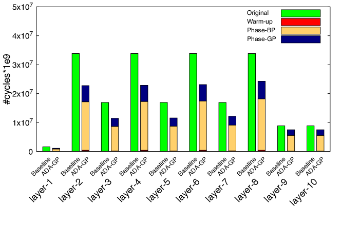
Figure 16. Characterization of ADA-GP in VGG13.

6.3. Performance Analysis

In the ADA-GP-MAX approach, during Phase BP, the forward pass (FW) of the predictor model can be computed simultaneously with the FW of the subsequent layer, as well as the backward pass (BW) of the predictor model alongside the BW of that layer. This method allows us to nearly eliminate the predictor model’s operation in Phase GP, but we must still determine the maximum between the original and predictor models. It is essential to wait for the current layer to complete its operation before proceeding to the next layer to avoid conflicts between the operations of different layers.

In the ADA-GP-Efficient method, the predictor’s weights are constantly stored in designated memory; however, there is no additional processing element (PE) to perform the predictor model’s operations in parallel with the original model’s operations. Consequently, the cost of each layer equals the sum of the original model and predictor model costs in distinct phases. Similar to the ADA-GP-MAX approach, the operations between layers are synchronized, initiating the subsequent layer’s operation only after the current layer’s operation is completed.

In the ADA-GP-LOW approach, there is no additional memory allocated for the predictor model weights, requiring us to load them after each original layer operation. Consequently, the expense associated with each layer should encompass the loading of predictor model weights and the storage of computed results. Nonetheless, following the loading process, the number of operations would be akin to the ADA-GP-Efficient approach.

Figures 17(a), 17(b), and 17(c) display the overall acceleration of ADA-GP-LOW, ADA-GP-Efficient and ADA-GP-MAX in comparison to the baseline system. In these figures, the baseline system represents a standard BP process utilizing the Weight-Stationary (WS) dataflow. The performance metrics are reported in relation to the dataset, as the model’s structure exhibits slight changes depending on the input size in different datasets. As demonstrated in these figures, ADA-GP-MAX can enhance the training by up to $1.51\times$, $1.51\times$, and $1.58\times$ for the Cifar10, Cifar100, and ImageNet datasets, respectively. Furthermore, it expedites the process by an average of $1.46\times$, $1.46\times$, and $1.48\times$ across all models for the Cifar10, Cifar100, and ImageNet datasets, respectively.

(a) Cifar10 dataset

(b) Cifar100 dataset

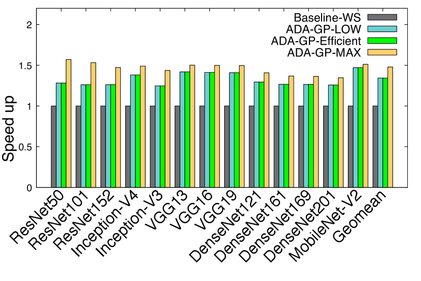
(c) ImageNet dataset

Figure 17. Speed up of ADA-GP over the baseline (BP) in Weight-Stationary (WS) dataflow.

We also perform analogous experiments for the Row Stationary (RS) dataflow. Figure 18 illustrates the overall acceleration of ADA-GP-LOW, ADA-GP-Efficient, and ADA-GP-MAX compared to the RS baseline. Figures 18(a), 18(b), and 18(c) indicate that ADA-GP-MAX can boost the training process by up to $1.48\times$ for each of the Cifar10, Cifar100, and ImageNet datasets. Additionally, it increases the training speed on average by $1.46\times$ across Cifar10 and Cifar100 datasets respectively, and $1.47\times$ in the ImageNet dataset.

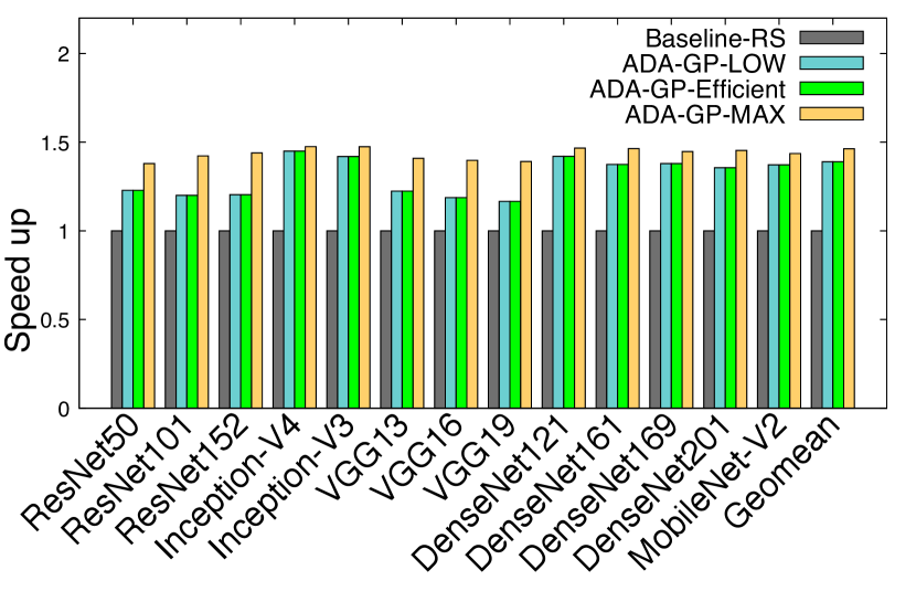
(a) Cifar10 dataset

(b) Cifar100 dataset

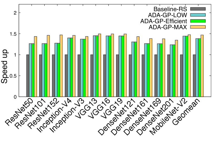
(c) ImageNet dataset

Figure 18. Speed up of ADA-GP over the baseline (BP) in Row-Stationary (RS) dataflow.

In a similar vein, we carried out additional experiments to demonstrate the acceleration of ADA-GP-LOW, ADA-GP-Efficient, and ADA-GP-MAX over the Input-Stationary (IS) dataflow baseline. Figure 19 presents a summary of these experimental results. Figures 19(a), 19(b), and 19(c) reveal that ADA-GP-MAX can enhance the training process by an average of $1.46\times$, $1.46\times$, and $1.48\times$ for the Cifar10, Cifar100, and ImageNet datasets, respectively.

(a) Cifar10 dataset

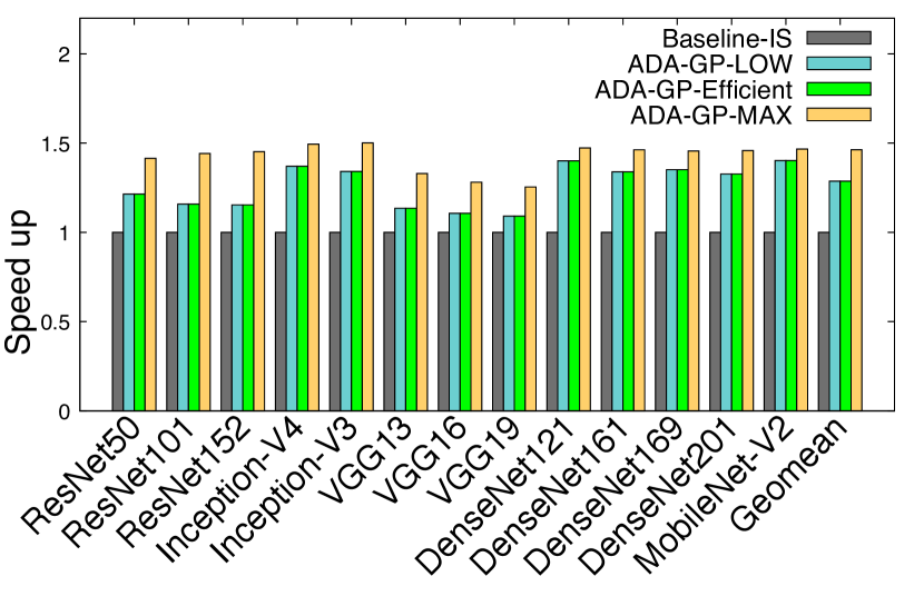
(b) Cifar100 dataset

(c) ImageNet dataset

Figure 19. Speed up of ADA-GP over the baseline (BP) in Input-Stationary (IS) dataflow.

6.4. Evaluation with Transformer and Object Detection Models

In this section, we employed the ADA-GP technique on Transformer, consisting of three encoding and decoding layers, as well as YOLO-v3 (Redmon and Farhadi, 2018) object detection models. We distinguish these models from other deep learning models due to the different employed datasets.

To assess our approach, for the Transformer model, we utilized the Multi30k (Elliott et al., 2016) English-German translation dataset. Table 2 shows the overall accuracy and performance comparison of ADA-GP with the baseline (BP) design.

Table 2. Accuracy and performance comparison between ADA-GP and the Baseline (BP) for Multi30k dataset.

	Val Acc.	loss	BLEU Score	#Cycles($\times 10^{9}$)
Baseline(BP)	52.42	1.61	33.52	1245.87
ADA-GP	52.14	1.65	33.4	1104.31

As demonstrated in Table 2, ADA-GP accelerates the training process of the Transformer by a factor of $1.13\times$. Furthermore, ADA-GP does not adversely impact the model’s performance and maintains the high accuracy of the Transformer model, achieving nearly identical BLEU Score (Papineni et al., 2002) results.

Furthermore, we employed the ADA-GP technique on the YOLO-v3 (Redmon and Farhadi, 2018) object detection model. Here, we utilized the Pascalvoc (Everingham et al., 2015) Visual Object Classes dataset. We set the initial learning rate to 3e-5, weight decay to 1e-4, and IOU threshold to 0.5. Table 3 shows the overall performance comparison of ADA-GP with the baseline (BP) design.

Table 3. Accuracy and performance comparison between ADA-GP and the Baseline (BP) for Pascalvoc dataset.

	Class Acc	Test MAP	#Cycles($\times 10^{9}$)
Baseline(BP)	83.03	0.4685	11490248
ADA-GP-Efficient	82.51	0.4674	9846579
ADA-GP-MAX	82.51	0.4674	9134071

As demonstrated in Table 2, ADA-GP accelerates the training process of the YOLO-v3 by a factor of $1.17\times$ and $1.26\times$ in ADA-GP-Efficient and ADA-GP-MAX, respectively. Furthermore, ADA-GP keeps the class accuracy high and achieves nearly identical Test MAP results.

6.5. Multi-Device Comparative Analysis

In this section, we evaluate the performance of the proposed ADA-GP relative to different baseline pipelining techniques using the ImageNet dataset in the context of multi-device hardware systems including GPipe (Huang et al., 2019), DAPPLE (Fan et al., 2021), and Chimera  (Li and Hoefler, 2021). We employ the scenario outlined in section 3.8 to compute the training acceleration. We consider a setup with four devices operating concurrently, where each mini-batch is split into four portions (macro-batch), and each device processes one macro-batch at a time. Similarly, we can implement ADA-GP across diverse multi-device hardware systems with varying numbers of devices, offering additional savings on top of their existing configurations. In this section, the duration of each time step is equivalent to the delay of the FW process in a single device for one macro-batch. Throughout the remainder of this section, we will employ this definition of a $step$ in our explanations.

6.5.1. Comparison with GPipe

As depicted in Figure 10, the standard GPipe method takes 21 steps to complete the training of $one$ batch. ADA-GP can significantly reduce computations in Phase GP by eliminating the conventional backpropagation process. Also, when transitioning from Phase GP to Phase BP, ADA-GP only requires 25 steps to finish the training of $two$ batches. Figure 20(a) depicts the overall acceleration of ADA-GP in comparison to the baseline GPipe method.

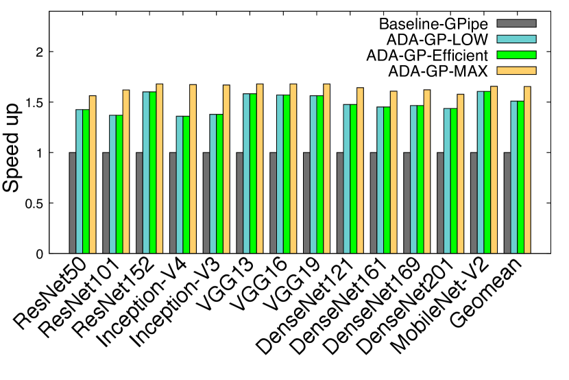
(a) Speed up over GPipe (Huang et al., 2019).

(b) Speed up over DAPPLE (Fan et al., 2021).

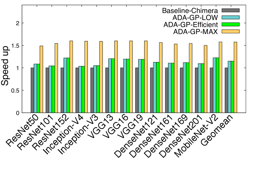
(c) Speed up over Chimera (Li and Hoefler, 2021).

Figure 20. Speed up of ADA-GP over the baseline pipelining techniques a) GPipe (Huang et al., 2019), b) DAPPLE (Fan et al., 2021), and c) Chimera (Li and Hoefler, 2021).

As seen in Figure 20(a), ADA-GP accelerates the training process for all deep learning models, achieving up to $1.68\times$ speedup and an average of $1.654\times$ improvement.

6.5.2. Comparison with DAPPLE

As illustrated in Figure 11, the DAPPLE method (Fan et al., 2021), similar to GPipe technique, requires 21 steps to complete the training of one batch. The timing of the ADA-GP when applied to DAPPLE also resembles that of the GPipe technique, taking into account the fact that the delay is associated with the DAPPLE design. Figure 20(b) demonstrates the extent of ADA-GP acceleration for various deep learning models compared to the baseline DAPPLE design, achieving a maximum speedup of $1.68\times$ and an average improvement of $1.654\times$.

6.5.3. Comparison with Chimera

The cutting-edge Chimera (Li and Hoefler, 2021) technique surpasses all prior methods, potentially addressing numerous gaps in deep learning model training. The Chimera approach manages to complete $one$ batch’s training in just 16 steps. By incorporating the ADA-GP into the Chimera method, not only do we retain all previous savings during Phase GP, but also when transitioning from Phase GP to Phase BP, the scheme necessitates merely 20 steps to finish training $two$ batches. Figure 20(c) provides the ADA-GP training acceleration for a range of deep learning models. As a result, the scheme effectively speeds up the Chimera training process for these models by up to $1.6\times$ and, on average, $1.575\times$.

6.6. Hardware Analysis

In this section, we discuss the resource usage and power consumption of ADA-GP for both ASIC and FPGA implementations. Additionally, we provide a detailed comparison of the energy consumption between ADA-GP and the baseline design. We employed CACTI (Naveen Muralimanohar, [n. d.]) to incorporate cache and memory access time, cycle time, area, leakage, and dynamic power model to calculate the design’s energy consumption.

6.6.1. ADA-GP Hardware Implementation Analysis

As mentioned in section 4.2, we proposed three unique designs: ADA-GP-LOW, ADA-GP-Effective, and ADA-GP-MAX, with the goal of balancing acceleration levels and hardware resources. In Table 4, we compare the resource usage and on-chip power consumption between ADA-GP designs and the baseline for the FPGA implementation.

Table 4. a) Resource usage and b) On-chip power consumption (watt) of ADA-GP designs vs baseline design in FPGA implementation.

(a) Resource Utilization

	#CLB	#CLB	#Block	#Block
	LUTs	Registers	RAMB36	RAMB18	#DSP48E1s
Baseline	472004	31402	1327	514	166
ADA-GP-LOW	489286	31856	1327	514	166
ADA-GP-Effic.	493171	31916	2407	514	166
ADA-GP-MAX	494080	37452	2407	514	246

(b) On-chip Power Consumption (watt)

		CLB		Block
	Clocks	Logic	Signals	RAM	DSPs	Static	Total
Baseline	0.046	0.42	0.842	0.244	0.009	2.032	3.712
ADA-GP-LOW	0.047	0.446	0.857	0.243	0.001	2.032	3.745
ADA-GP-Effic.	0.052	0.421	0.852	0.339	0.001	2.06	3.844
ADA-GP-MAX	0.055	0.426	0.857	0.339	0.001	2.059	3.856

As illustrated in Table 4, the ADA-GP-LOW, ADA-GP-Effective, and ADA-GP-MAX designs result in a power increase of only 0.8%, 3.5%, and 3.8%, respectively. This rise in power consumption is due to the additional hardware incorporated in the various designs. We conducted another experiment with the baseline and ADA-GP-MAX having the same power. This makes a 10% increase in the number of PEs in the baseline and an average speedup of 4.31%, 4.3%, and 4.47% for Cifar10, Cifar100, and ImageNet datasets.

Table 5 contrasts the area and power consumption of the different ADA-GP designs with the baseline in the ASIC implementation.

Table 5. a) Area and b) power consumption (watt) of ADA-GP designs vs baseline design in ASIC implementation.

(a) Area

			Net	Total	Total
	Combinational	Buf/Inv	Intercon.	Cell	Area
Baseline	2331250	272483	436615	2546076	2982691
ADA-GP-LOW	2375188	277261	445371	2590583	3035954
ADA-GP-Effic.	2405881	275783	440031	2622858	3062890
ADA-GP-MAX	2512057	287076	460157	2770979	3231136

(b) Power ($\mu$ watt)

	Internal	Switching	Leakage	Total
Baseline	2.26E+04	1.72E+03	1.99E+05	2.24E+05
ADA-GP-LOW	2.25E+04	1.67E+03	2.02E+05	2.26E+05
ADA-GP-Effic.	2.27E+04	1.80E+03	2.00E+05	2.25E+05
ADA-GP-MAX	2.80E+04	2.42E+03	2.23E+05	2.54E+05

As depicted in Table 5, the ADA-GP-LOW, ADA-GP-Efficient, and ADA-GP-MAX designs lead to an increase in the final design area by 1.7%, 2.6%, and 8.3%, respectively. This also results in a rise in the design power. Similar to FPGA implementation we experimented with the baseline and ADA-GP-MAX having the same area. This results in 11% additional PE in the baseline and an average speedup of 4.63%, 4.61%, and 5.53% for Cifar10, Cifar100, and ImageNet datasets.

6.6.2. Energy Consumption Analysis

In Figure 21, the energy consumption associated with memory access during the training process for both the baseline and ADA-GP  methods is compared. As a result, ADA-GP  enhances energy efficiency for all models, resulting in an average reduction of energy consumption by 34%.

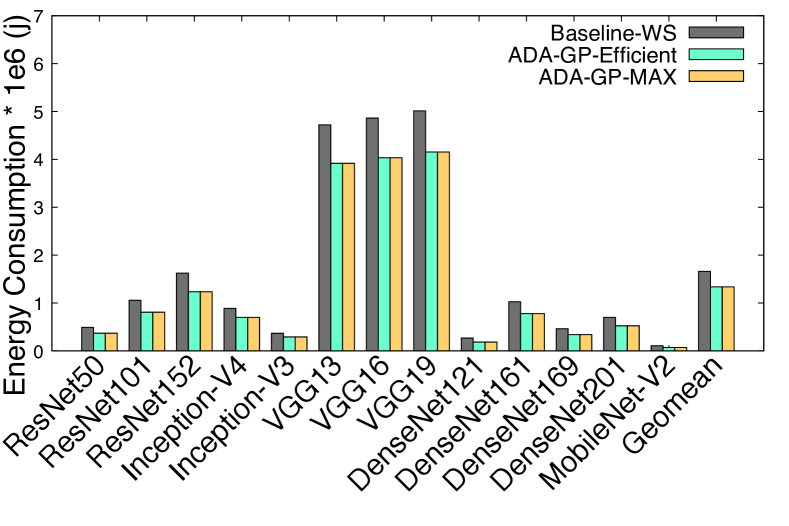
Figure 21. The energy consumption comparison between baseline back propagation and ADA-GP designs.

It is worth mentioning that the presented results do not take into account the savings achieved by reducing the number of synchronization steps, but only reflect the savings from reducing the number of memory read/write operations.

7. Conclusions

In this paper, we proposed ADA-GP, the first approach to use gradient prediction to improve the performance of DNN training while maintaining accuracy. ADA-GP warms up the predictor model during the initial few epochs. After that ADA-GP alternates between using backpropagated gradients and predicted gradients for updating weights. As the training proceeds, ADA-GP adaptively decides when and for how long gradient prediction should be used. ADA-GP uses a single predictor model for all layers and uses a novel tensor reorganization to predict a large number of gradients. We experimented with fifteen DNN models using three different datasets - Cifar10, Cifar100, and ImageNet. Our results indicate that ADA-GP can achieve an average speed up of 1.47× with similar or even higher accuracy than the baseline models. Moreover, due to the reduced off-chip memory accesses during the weight updates, ADA-GP consumes 34% less energy compared to the baseline accelerator.

References

- (1)
- Balduzzi et al. (2015) David Balduzzi, Hastagiri Vanchinathan, and Joachim Buhmann. 2015. Kickback cuts backprop’s red-tape: Biologically plausible credit assignment in neural networks. In Proceedings of the AAAI Conference on Artificial Intelligence, Vol. 29.
- Belilovsky et al. (2020) Eugene Belilovsky, Michael Eickenberg, and Edouard Oyallon. 2020. Decoupled greedy learning of cnns. In International Conference on Machine Learning. PMLR, 736–745.
- Brown et al. (2020) Tom B. Brown, Benjamin Mann, Nick Ryder, Melanie Subbiah, Jared Kaplan, Prafulla Dhariwal, Arvind Neelakantan, Pranav Shyam, Girish Sastry, Amanda Askell, Sandhini Agarwal, Ariel Herbert-Voss, Gretchen Krueger, Tom Henighan, Rewon Child, Aditya Ramesh, Daniel M. Ziegler, Jeffrey Wu, Clemens Winter, Christopher Hesse, Mark Chen, Eric Sigler, Mateusz Litwin, Scott Gray, Benjamin Chess, Jack Clark, Christopher Berner, Sam McCandlish, Alec Radford, Ilya Sutskever, and Dario Amodei. 2020. Language Models are Few-Shot Learners. arXiv:2005.14165 [cs.CL]
- Chakradhar et al. (2010) Srimat Chakradhar, Murugan Sankaradas, Venkata Jakkula, and Srihari Cadambi. 2010. A dynamically configurable coprocessor for convolutional neural networks. In Proceedings of the 37th annual international symposium on Computer architecture. 247–257.
- Chen et al. (2016) Y. Chen, J. Emer, and V. Sze. 2016. Eyeriss: A Spatial Architecture for Energy-Efficient Dataflow for Convolutional Neural Networks. In 2016 ACM/IEEE 43rd Annual International Symposium on Computer Architecture (ISCA). 367–379. https://doi.org/10.1109/ISCA.2016.40
- Chen et al. (2017) Yu Chen, Joel Emer, and Vivienne Sze. 2017. Using Dataflow to Optimize Energy Efficiency of Deep Neural Network Accelerators. IEEE Micro 37, 3 (2017), 12–21. https://doi.org/10.1109/MM.2017.54
- Czarnecki et al. (2017a) Wojciech M Czarnecki, Simon Osindero, Max Jaderberg, Grzegorz Swirszcz, and Razvan Pascanu. 2017a. Sobolev training for neural networks. Advances in neural information processing systems 30 (2017).
- Czarnecki et al. (2017b) Wojciech Marian Czarnecki, Grzegorz Świrszcz, Max Jaderberg, Simon Osindero, Oriol Vinyals, and Koray Kavukcuoglu. 2017b. Understanding synthetic gradients and decoupled neural interfaces. In International Conference on Machine Learning. PMLR, 904–912.
- Deng et al. (2009) J. Deng, W. Dong, R. Socher, L.-J. Li, K. Li, and L. Fei-Fei. 2009. ImageNet: A Large-Scale Hierarchical Image Database. In CVPR09.
- Du et al. (2015) Zidong Du, Robert Fasthuber, Tianshi Chen, Paolo Ienne, Ling Li, Tao Luo, Xiaobing Feng, Yunji Chen, and Olivier Temam. 2015. ShiDianNao: Shifting vision processing closer to the sensor. In Proceedings of the 42nd Annual International Symposium on Computer Architecture. 92–104.
- Elliott et al. (2016) Desmond Elliott, Stella Frank, Khalil Sima’an, and Lucia Specia. 2016. Multi30K: Multilingual English-German Image Descriptions. In Proceedings of the 5th Workshop on Vision and Language. Association for Computational Linguistics, Berlin, Germany, 70–74. https://doi.org/10.18653/v1/W16-3210
- Everingham et al. (2015) M. Everingham, S. M. A. Eslami, L. Van Gool, C. K. I. Williams, J. Winn, and A. Zisserman. 2015. The Pascal Visual Object Classes Challenge: A Retrospective. International Journal of Computer Vision 111, 1 (Jan. 2015), 98–136.
- Fan et al. (2021) Shiqing Fan, Yi Rong, Chen Meng, Zongyan Cao, Siyu Wang, Zhen Zheng, Chuan Wu, Guoping Long, Jun Yang, Lixue Xia, et al. 2021. DAPPLE: A pipelined data parallel approach for training large models. In Proceedings of the 26th ACM SIGPLAN Symposium on Principles and Practice of Parallel Programming. 431–445.
- Gokhale et al. (2014) Vinayak Gokhale, Jonghoon Jin, Aysegul Dundar, Berin Martini, and Eugenio Culurciello. 2014. A 240 g-ops/s mobile coprocessor for deep neural networks. In Proceedings of the IEEE conference on computer vision and pattern recognition workshops. 682–687.
- Goyal et al. (2017) Priya Goyal, Piotr Dollár, Ross Girshick, Pieter Noordhuis, Lukasz Wesolowski, Aapo Kyrola, Andrew Tulloch, Yangqing Jia, and Kaiming He. 2017. Accurate, large minibatch sgd: Training imagenet in 1 hour. arXiv preprint arXiv:1706.02677 (2017).
- Grigorescu et al. (2020) Sorin Grigorescu, Bogdan Trasnea, Tiberiu Cocias, and Gigel Macesanu. 2020. A survey of deep learning techniques for autonomous driving. Journal of Field Robotics 37, 3 (apr 2020), 362–386. https://doi.org/10.1002/rob.21918
- He et al. (2016) Kaiming He, Xiangyu Zhang, Shaoqing Ren, and Jian Sun. 2016. Deep residual learning for image recognition. In Proceedings of the IEEE conference on computer vision and pattern recognition. 770–778.
- Howard et al. (2018) Andrew Howard, Andrey Zhmoginov, Liang-Chieh Chen, Mark Sandler, and Menglong Zhu. 2018. Inverted residuals and linear bottlenecks: Mobile networks for classification, detection and segmentation. (2018).
- Huang et al. (2017) Gao Huang, Zhuang Liu, Laurens Van Der Maaten, and Kilian Q Weinberger. 2017. Densely connected convolutional networks. In Proceedings of the IEEE conference on computer vision and pattern recognition. 4700–4708.
- Huang et al. (2019) Yanping Huang, Youlong Cheng, Ankur Bapna, Orhan Firat, Dehao Chen, Mia Chen, HyoukJoong Lee, Jiquan Ngiam, Quoc V Le, Yonghui Wu, et al. 2019. Gpipe: Efficient training of giant neural networks using pipeline parallelism. Advances in neural information processing systems 32 (2019).
- Huo et al. (2018a) Zhouyuan Huo, Bin Gu, and Heng Huang. 2018a. Training neural networks using features replay. Advances in Neural Information Processing Systems 31 (2018).
- Huo et al. (2018b) Zhouyuan Huo, Bin Gu, Heng Huang, et al. 2018b. Decoupled parallel backpropagation with convergence guarantee. In International Conference on Machine Learning. PMLR, 2098–2106.
- Jaderberg et al. (2017) Max Jaderberg, Wojciech Marian Czarnecki, Simon Osindero, Oriol Vinyals, Alex Graves, David Silver, and Koray Kavukcuoglu. 2017. Decoupled neural interfaces using synthetic gradients. In International conference on machine learning. PMLR, 1627–1635.
- Jain et al. (2020) Arpan Jain, Ammar Ahmad Awan, Asmaa M Aljuhani, Jahanzeb Maqbool Hashmi, Quentin G Anthony, Hari Subramoni, Dhableswar K Panda, Raghu Machiraju, and Anil Parwani. 2020. Gems: Gpu-enabled memory-aware model-parallelism system for distributed dnn training. In SC20: International Conference for High Performance Computing, Networking, Storage and Analysis. IEEE, 1–15.
- Janfaza et al. (2023) Vahid Janfaza, Kevin Weston, Moein Razavi, Shantanu Mandal, Farabi Mahmud, Alex Hilty, and Abdullah Muzahid. 2023. MERCURY: Accelerating DNN Training By Exploiting Input Similarity. In 2023 IEEE International Symposium on High-Performance Computer Architecture (HPCA). 638–650. https://doi.org/10.1109/HPCA56546.2023.10071051
- Jia et al. (2019) Zhihao Jia, Matei Zaharia, and Alex Aiken. 2019. Beyond Data and Model Parallelism for Deep Neural Networks. Proceedings of Machine Learning and Systems 1 (2019), 1–13.
- Krizhevsky (2014) Alex Krizhevsky. 2014. One weird trick for parallelizing convolutional neural networks. arXiv preprint arXiv:1404.5997 (2014).
- Krizhevsky et al. (2009) Alex Krizhevsky, Geoffrey Hinton, et al. 2009. Learning multiple layers of features from tiny images. (2009).
- Krizhevsky et al. (2012) Alex Krizhevsky, Ilya Sutskever, and Geoffrey E. Hinton. 2012. ImageNet Classification with Deep Convolutional Neural Networks. In Proceedings of the 25th International Conference on Neural Information Processing Systems - Volume 1 (Lake Tahoe, Nevada) (NIPS’12). Curran Associates Inc., Red Hook, NY, USA, 1097–1105.
- Kwon et al. (2018) Hyoukjun Kwon, Ananda Samajdar, and Tushar Krishna. 2018. MAERI: Enabling Flexible Dataflow Mapping over DNN Accelerators via Reconfigurable Interconnects. SIGPLAN Not. 53, 2 (2018), 461–475. https://doi.org/10.1145/3296957.3173176
- LeCun et al. (2012) Yann A. LeCun, Léon Bottou, Genevieve B. Orr, and Klaus-Robert Müller. 2012. Efficient BackProp. Springer Berlin Heidelberg, Berlin, Heidelberg, 9–48. https://doi.org/10.1007/978-3-642-35289-8_3
- Li et al. (2020) Shigang Li, Tal Ben-Nun, Salvatore Di Girolamo, Dan Alistarh, and Torsten Hoefler. 2020. Taming unbalanced training workloads in deep learning with partial collective operations. In Proceedings of the 25th ACM SIGPLAN Symposium on Principles and Practice of Parallel Programming. 45–61.
- Li and Hoefler (2021) Shigang Li and Torsten Hoefler. 2021. Chimera: efficiently training large-scale neural networks with bidirectional pipelines. In Proceedings of the International Conference for High Performance Computing, Networking, Storage and Analysis. 1–14.
- Lillicrap et al. (2016) Timothy P Lillicrap, Daniel Cownden, Douglas B Tweed, and Colin J Akerman. 2016. Random synaptic feedback weights support error backpropagation for deep learning. Nature communications 7, 1 (2016), 13276.
- Miyato et al. (2017) Takeru Miyato, Daisuke Okanohara, Shin-ichi Maeda, and Masanori Koyama. 2017. Synthetic gradient methods with virtual forward-backward networks. (2017).
- Naveen Muralimanohar ([n. d.]) Vaishnav Srinivas Naveen Muralimanohar, Ali Shafiee. [n. d.]. CACTI. http://www.hpl.hp.com/research/cacti/
- Nøkland (2016) Arild Nøkland. 2016. Direct feedback alignment provides learning in deep neural networks. Advances in neural information processing systems 29 (2016).
- Papineni et al. (2002) Kishore Papineni, Salim Roukos, Todd Ward, and Wei-Jing Zhu. 2002. Bleu: a method for automatic evaluation of machine translation. In Proceedings of the 40th annual meeting of the Association for Computational Linguistics. 311–318.
- Paszke et al. (2019) Adam Paszke, Sam Gross, Francisco Massa, Adam Lerer, James Bradbury, Gregory Chanan, Trevor Killeen, Zeming Lin, Natalia Gimelshein, Luca Antiga, et al. 2019. Pytorch: An imperative style, high-performance deep learning library. Advances in neural information processing systems 32 (2019).
- Peemen et al. (2013) Maurice Peemen, Arnaud AA Setio, Bart Mesman, and Henk Corporaal. 2013. Memory-centric accelerator design for convolutional neural networks. In 2013 IEEE 31st International Conference on Computer Design (ICCD). IEEE, 13–19.
- Qiao et al. (2019) Tingting Qiao, Jing Zhang, Duanqing Xu, and Dacheng Tao. 2019. Learn, Imagine and Create: Text-to-Image Generation from Prior Knowledge. In Advances in Neural Information Processing Systems, H. Wallach, H. Larochelle, A. Beygelzimer, F. d'Alché-Buc, E. Fox, and R. Garnett (Eds.), Vol. 32. Curran Associates, Inc. https://proceedings.neurips.cc/paper_files/paper/2019/file/d18f655c3fce66ca401d5f38b48c89af-Paper.pdf
- Redmon and Farhadi (2018) Joseph Redmon and Ali Farhadi. 2018. Yolov3: An incremental improvement. arXiv preprint arXiv:1804.02767 (2018).
- Sankaradas et al. (2009) Murugan Sankaradas, Venkata Jakkula, Srihari Cadambi, Srimat Chakradhar, Igor Durdanovic, Eric Cosatto, and Hans Peter Graf. 2009. A massively parallel coprocessor for convolutional neural networks. In 2009 20th IEEE International Conference on Application-specific Systems, Architectures and Processors. IEEE, 53–60.
- Sergeev and Del Balso (2018) Alexander Sergeev and Mike Del Balso. 2018. Horovod: fast and easy distributed deep learning in TensorFlow. arXiv preprint arXiv:1802.05799 (2018).
- Silver et al. (2017) David Silver, Thomas Hubert, Julian Schrittwieser, Ioannis Antonoglou, Matthew Lai, Arthur Guez, Marc Lanctot, Laurent Sifre, Dharshan Kumaran, Thore Graepel, Timothy Lillicrap, Karen Simonyan, and Demis Hassabis. 2017. Mastering Chess and Shogi by Self-Play with a General Reinforcement Learning Algorithm. arXiv:1712.01815 [cs.AI]
- Simonyan and Zisserman (2014) Karen Simonyan and Andrew Zisserman. 2014. Very deep convolutional networks for large-scale image recognition. arXiv preprint arXiv:1409.1556 (2014).
- Synopsys ([n. d.]) Synopsys. [n. d.]. Desgin Compiler. https://www.synopsys.com/implementation-and-signoff/rtl-synthesis-test/dc-ultra.html
- Sze et al. (2017) Vivienne Sze, Yu-Hsin Chen, Tien-Ju Yang, and Joel S Emer. 2017. Efficient processing of deep neural networks: A tutorial and survey. Proc. IEEE 105, 12 (2017), 2295–2329.
- Szegedy et al. (2016a) Christian Szegedy, Sergey Ioffe, Vincent Vanhoucke, and Alex Alemi. 2016a. Inception-v4, Inception-ResNet and the Impact of Residual Connections on Learning. arXiv:1602.07261 [cs.CV]
- Szegedy et al. (2016b) Christian Szegedy, Vincent Vanhoucke, Sergey Ioffe, Jon Shlens, and Zbigniew Wojna. 2016b. Rethinking the inception architecture for computer vision. In Proceedings of the IEEE conference on computer vision and pattern recognition. 2818–2826.
- Vaswani et al. (2017a) Ashish Vaswani, Noam Shazeer, Niki Parmar, Jakob Uszkoreit, Llion Jones, Aidan N. Gomez, Lukasz Kaiser, and Illia Polosukhin. 2017a. Attention Is All You Need. https://doi.org/10.48550/ARXIV.1706.03762
- Vaswani et al. (2017b) Ashish Vaswani, Noam Shazeer, Niki Parmar, Jakob Uszkoreit, Llion Jones, Aidan N Gomez, Łukasz Kaiser, and Illia Polosukhin. 2017b. Attention is all you need. Advances in neural information processing systems 30 (2017).
- wikipedia ([n. d.]) wikipedia. [n. d.]. MAPE. https://en.wikipedia.org/wiki/Mean_absolute_percentage_error
- Xilinx ([n. d.]) Xilinx. [n. d.]. Vivado. https://www.xilinx.com/products/design-tools/vivado.html
- Xilinx (2007) Xilinx. 2007. Virtex 7 FPGA. https://www.xilinx.com/products/silicon-devices/fpga/virtex-7.html
- Xu et al. (2017) David Xu, Andrew Clappison, Cameron Seth, and Jeff Orchard. 2017. Symmetric predictive estimator for biologically plausible neural learning. IEEE Transactions on Neural Networks and Learning Systems 29, 9 (2017), 4140–4151.
- You et al. (2018) Yang You, Zhao Zhang, Cho-Jui Hsieh, James Demmel, and Kurt Keutzer. 2018. Imagenet training in minutes. In Proceedings of the 47th International Conference on Parallel Processing. 1–10.
- Zhuang et al. (2021) Huiping Zhuang, Yi Wang, Qinglai Liu, and Zhiping Lin. 2021. Fully decoupled neural network learning using delayed gradients. IEEE transactions on neural networks and learning systems 33, 10 (2021), 6013–6020.