SparseFit: Few-shot Prompting with Sparse Fine-tuning for Jointly Generating Predictions and Natural Language Explanations

Abstract

Explaining the decisions of neural models is crucial for ensuring their trustworthiness at deployment time. Using Natural Language Explanations (NLEs) to justify a model’s predictions has recently gained increasing interest. However, this approach usually demands large datasets of human-written NLEs for the ground-truth answers, which are expensive and potentially infeasible for some applications. For models to generate high-quality NLEs when only a few NLEs are available, the fine-tuning of Pre-trained Language Models (PLMs) in conjunction with prompt-based learning recently emerged. However, PLMs typically have billions of parameters, making fine-tuning expensive. We propose SparseFit, a sparse few-shot fine-tuning strategy that leverages discrete prompts to jointly generate predictions and NLEs. We experiment with SparseFit on the T5 model and four datasets and compare it against state-of-the-art parameter-efficient fine-tuning techniques. We perform automatic and human evaluations to assess the quality of the model-generated NLEs, finding that fine-tuning only $6.8\%$ of the model parameters leads to competitive results for both the task performance and the quality of the NLEs.

1 Introduction

Despite the tremendous success of neural networks  (Chowdhery et al., 2022; Brown et al., 2020), these models usually lack human-intelligible explanations for their predictions, which are paramount for ensuring their trustworthiness. Building neural models that explain their predictions in natural language has seen increasing interest in recent years Wiegreffe and Marasovic (2021). Natural Language Explanations (NLEs) are generally easy to interpret by humans and more expressive than other types of explanations such as saliency maps (Wallace et al., 2019; Wiegreffe and Marasovic, 2021). However, a significant downside of these models is that they require large datasets of human-written NLEs at training time, which can be expensive and time-consuming to collect. To this end, few-shot learning of NLEs has recently emerged Marasovic et al. (2022); Yordanov et al. (2022). However, current techniques involve fine-tuning the entire model with a few training NLE examples. This is computationally expensive since current NLE models can have billions of parameters Schwartz et al. (2020).

In this paper, we investigate whether sparse fine-tuning (i.e. fine-tuning only a subset of parameters), in conjunction with prompt-based learning, (i.e. textual instructions given to a PLM (Liu et al., 2021)) can help in scenarios with limited availability of training instances with labels and NLEs. While sparse fine-tuning has been used in natural language processing (NLP) (Houlsby et al., 2019; IV et al., 2022), to our knowledge, our work is the first to analyze sparse fine-tuning in the context of jointly generating predictions and NLEs. Moreover, we extend the existing sparse fine-tuning strategy that looks only at bias terms Zaken et al. (2022) to a comprehensive list of all layers and pairs of layers.

Thus, we propose SparseFit, an efficient few-shot prompt-based training regime for models generating both predictions and NLEs for their predictions. We experiment with SparseFit on two pre-trained language models (PLMs) that have previously shown high performance on task performance and NLE generation; namely T5 Raffel et al. (2020) and UnifiedQA Dong et al. (2019). We test our approach on four popular NLE datasets: e-SNLI (Camburu et al., 2018), ECQA (Aggarwal et al., 2021), SBIC (Sap et al., 2020), and ComVE (Wang et al., 2019), and evaluate both the task performance and the quality of the generated NLEs, the latter with both automatic metrics and human evaluation. Overall, SparseFit shows competitive performance in few-shot learning settings with 48 training instances. For example, fine-tuning only the Normalization Layer together with the Self-attention Query Layer, which amounts to $6.84\%$ of the model’s parameters, consistently gave the best performance (penalized by the number of fine-tuned parameters) on both T5 and UnifiedQA over all four datasets. Remarkably, it outperforms the current state-of-the-art (SOTA) parameters-efficient fine-tuning (PEFT) models in terms of both task performance and quality of generated NLEs in three of the four datasets. Furthermore, we find that fine-tuning other model components that comprise a small fraction of the parameters also consistently leads to competitive results; these components include the Self-attention Query Layer (${\sim}6.8\%$ of the parameters), entire Self-attention Layer (${\sim}20\%$), and the Dense layers (${\sim}27\%$). Therefore, we conclude that few-shot sparse fine-tuning of large PLMs can achieve results that are competitive with fine-tuning the entire model.

2 Related Work

Few-shot learning refers to training models with limited labelled data for a given task Finn et al. (2017); Vinyals et al. (2016); Lampert et al. (2009). It has been successfully applied to several tasks such as image captioning (Dong et al., 2018), object classification (Ren et al., 2018), behavioral bio-metrics (Solano et al., 2020), neural network architecture search (Brock et al., 2018), graph node classification (Satorras and Estrach, 2018), and language modeling (Vinyals et al., 2016). Large LMs have shown impressive skills to learn in few-shot scenarios (Brown et al., 2020; Chowdhery et al., 2022) thanks to the size of the pre-training corpora and the statistical capacity of the models (Izacard et al., 2022). For instance, PaLM (Chowdhery et al., 2022) has 540B parameters trained with the Pathways system (Barham et al., 2022) over 780B tokens.

Parameter-efficient Fine-tuning

Using fine-tuning, large LMs have shown breakthrough language understanding and generation capabilities in a wide range of domains (Raffel et al., 2020; Brown et al., 2020; Chowdhery et al., 2022). However, in NLP, the up-stream model (i.e. the model to be fine-tuned) is commonly a large LM with millions of parameters, such as T5 (Raffel et al., 2020), BERT (Devlin et al., 2019), or GPT-3 (Radford et al., 2018), which makes them computationally expensive to fine-tune. This led to strategies where only a small subset of the model parameters is fine-tuned to keep competitive performance in the downstream task. The approaches that fine-tune only a small set of the PLM parameters, or an extra small set of parameters, are known in the literature as Parameter-efficient Fine-tuning (PEFT). In this regard, Houlsby et al. (2019) developed a strategy that injects model-independent modules, referred to as adapters, with only a few trainable parameters. In their approach, the parameters of the original LM remain fixed while only the parameters of the adapter layers are fine-tuned. Later, Hu et al. (2022) developed LoRA, a technique that injects trainable low-rank matrices in the transformer architecture while freezing the pre-trained model weights. With a different approach in mind, Li and Liang (2021) introduced Prefix-Tuning, a strategy that focuses on adding a small task-specific vector to the input, so the frozen PLM can adapt its knowledge to further downstream tasks. More recently, Zaken et al. (2022) presented BitFit, a novel approach aimed at only fine-tuning the bias terms in each layer of a transformer-based LM. We extend their work to fine-tuning each of the layers/blocks and pairs of them.

Explainability of Neural Models

Several approaches have been proposed in the literature to bring a degree of explainability to the predictions of neural models, using different forms of explanations, such as (1) Feature-based explanations (Ribeiro et al., 2016; Lundberg and Lee, 2017; Shrikumar et al., 2017; Yoon et al., 2019; Sha et al., 2021), (2) Natural Language Explanations (Camburu et al., 2018; Marasović et al., 2020; Kayser et al., 2022; Majumder et al., 2022), (3) Counterfactual explanations (Akula et al., 2020), and (4) Surrogate explanations (Alaa and van der Schaar, 2019). In this paper, we focus on models that provide NLEs, i.e., free-form text stating the reasons behind a prediction. Being in natural language, NLEs should be easy to interpret by humans and more expressive than other types of explanations as they can present arguments that are not present in the input (Wiegreffe and Marasovic, 2021; Camburu et al., 2021; Kaur et al., 2020). NLEs have been applied to several domains such as question answering (Narang et al., 2020), natural language inference (Camburu et al., 2018), recommendation systems (Chen et al., 2021), reinforcement learning (Ehsan et al., 2018), medical imagining (Kayser et al., 2022), visual-textual reasoning (Park et al., 2018; Hendricks et al., 2018; Kayser et al., 2021; Majumder et al., 2022), self-driving cars (Kim et al., 2018), and solving mathematical problems (Ling et al., 2017).

To make neural models capable of generating accurate NLEs, the most common approach consists of annotating predictions with human-written explanations and training models to generate the NLEs by casting them as a sequence generation task (Camburu et al., 2018). However, gathering large datasets with human-written NLEs is expensive and time-consuming. Recently, Marasovic et al. (2022) introduced the FEB benchmark for few-shot learning of NLEs and a prompt-based fine-tuning strategy, which we use as a baseline in our work. Yordanov et al. (2022) proposed a vanilla transfer learning strategy to learn from a few NLEs but abundant labels in a task (child task), given that the model was pre-trained over a vast number of NLEs belonging to a different task in another domain (parent task). Their results show that generating out-of-domain NLEs via transfer learning from a parent task outperforms single-task training from scratch for NLE generation.

3 SparseFit

We propose SparseFit, an efficient few-shot NLE training strategy that focuses on fine-tuning only a subset of parameters in a large LM.

SparseFit is inspired by (1) Marasovic et al. (2022), who used fine-tuning and prompts to do few-shot learning of labels and NLEs; and (2) BitFit Zaken et al. (2022), who showed that fine-tuning only the bias terms in the BERT language model (Devlin et al., 2019) leads to competitive (and sometimes better) performance than fine-tuning the entire model. We extend BitFit and propose to explore the fine-tuning of all the different components (i.e., layers or blocks) in the model’s transformer architecture. In particular, we study the self-rationalization performance after fine-tuning the following components in the T5 model: (1) the encoder blocks, (2) the decoder blocks, (3) the language model head, (4) the attention layers, (5) the feed-forward networks, (6) the normalization layer, and (7) all 31 pairs of the above components that do not contain the encoder and decoder due to their size (see Appendix B).

Considering that the UnifiedQA model’s architecture is the same as the one in T5, the interpretation of active parameters holds for UnifiedQA. Our goal is to find a general recommendation on what component, or pair of components, should be fine-tuned to keep competitive performance while updating a minimum number of parameters.

When fine-tuning any model component or pair of components, we freeze all other parameters of the LM and train the LM to conditionally generate a text in the form of “[label] because [explanation]”.

Encoder

The encoder in T5 is composed of $N$ transformer blocks, each composed of three layers: self-attention, position-wise fully connected layer, and layer normalization. The number of blocks depends on the size of the T5 model ($N=12$ blocks for T5-base, $N=24$ for T5-large, and $N=36$ for T5-3B). The encoder accounts for roughly $41\%$ of the model parameters.

Decoder

The decoder accounts for roughly $54\%$ of T5 model parameters. In addition to the self-attention, fully connected layer, and layer normalization, it also includes an encoder-decoder attention layer in its blocks, which we fine-tune as part of fine-tuning the decoder.

LM Head

On top of the decoder, T5 has a language modeling head for generating text based on the corpus. The LM head accounts for roughly $5\%$ of total model parameters.

Attention Layer

Each of the transformer blocks starts with a self-attention layer. There are three types of parameters in the self-attention layer, namely, for computing the query matrix $Q$, the key matrix $K$, and the value matrix $V$. We propose to explore the fine-tuning of each self-attention matrix as a SparseFit configuration. We also explore fine-tuning the entire Self-attention Layer ($Q$, $K$, $V$). On average, the percentage of trainable parameters associated with each matrix accounts for roughly $6\%$ of model parameters. Note that the attention parameters in the encoder-decoder attention are not updated in this setting (they are only updated together with the decoder).

Layer Normalization

The normalization layers are intended to improve the training speed of the models Ba et al. (2016). The T5 model includes two Layer Normalization components per block, one after the self-attention layer and one after the feed-forwards networks. Unlike the original paper for layer normalization (Ba et al., 2016), the T5 model uses a simplified version of the layer normalization that only re-scales the activations. The percentage of learnable weights in the layer normalization is roughly $0.2\%$ of the parameters.

4 Experiments

Datasets

We follow the FEB benchmark for few-shot learning of NLEs (Marasovic et al., 2022), and consider four NLE datasets: e-SNLI for natural language inference (Camburu et al., 2018), ECQA for multiple-choice question answering (Aggarwal et al., 2021), ComVE for commonsense classification (Wang et al., 2019), and SBIC for offensiveness classification (Sap et al., 2020).

Few-shot Learning Data Splits

We also follow the few-shot evaluation protocol used by Marasovic et al. (2022). We use their 60 train-validation splits to run our experiments. Each experiment is run with 48 examples in the training set and 350 examples in the validation set. Note that, depending on the dataset, the number of training examples per label varies: e-SNLI has 16 examples for each label, ECQA 48, SBIC 24, and ComVE 24, resulting in 48 training examples for all datasets.

Training Procedure

Following Marasovic et al. (2022), we fine-tune T5 (Raffel et al., 2020) and UnifiedQA (Khashabi et al., 2020). Depending on the setup, the gradients could be activated for specific parameters (SparseFit) or the entire model (baseline). We report our experimental results for the baseline and observe a behavior consistent with the one reported by Marasovic et al. (2022). Additionally, to compare to with other PEFT baselines, we also adapted LoRA Hu et al. (2022) and Prefix-Tuning Li and Liang (2021) for NLEs. For the SparseFit configurations, we fine-tune each component (or pair) for 25 epochs with a batch size of 4 samples. Similarly to Marasovic et al. (2022), we use the AdamW optimizer (Loshchilov and Hutter, 2019) with a fixed learning rate of $3\times 10^{-5}$. The inference is performed using conditional text generation on the validation set. During the generation process, we only constrain the maximum length of the generated NLE. Training and inference time for each split is $23.2$ minutes on average, running on an academic HPC cluster of NVIDIA P100 and V100 GPUs.

Automatic Evaluation

The evaluation considers both the task accuracy and the quality of the generated NLEs. To automatically evaluate the quality of the NLEs, we follow Marasovic et al. (2022) and use the BERTScore (Zhang et al., 2019), which was shown by Kayser et al. (2021) to correlate best with human evaluation in NLEs. As in Marasovic et al. (2022), we compute a normalized BERTScore that assigns a zero score to empty NLEs, or NLEs of incorrectly predicted samples (since one would not expect, nor want, an NLE to be plausible if the prediction was wrong). In summary, we report the averages and standard deviations of the accuracy and the normalized BERTScore over the 60 train-validation splits for each fine-tuning configuration.

Human Evaluation

In addition to the normalized BERTScore, we also perform a smaller-scale human evaluation to assess the quality of NLEs for the best-performing SparseFit configurations. We use the NLEs associated with the first 30 correctly predicted samples in each validation set in the training for human evaluation. To make the evaluation more robust, 30 samples were chosen to be balanced in the number of classes. Our human evaluation framework follows those of Kayser et al. (2021); Marasovic et al. (2022). For the NLE quality assessment, each annotator is asked to answer the following question: “Does the explanation justify the answer?" and should select one of four possible answers: yes, weak yes, weak no, or no.

We also ask the annotators to identify the main shortcomings, if any, of the generated NLEs. The possible shortcomings categories are (1) nonsensical, (2) contradictory, (3) lack of explanation, (4) incomplete explanation, (5) input repetition, (6) hallucination, (7) extra words at the end, (8) true but uncorrelated, (9) inaccurate, and (10) one word. An author and a third-party annotator (with an MSc degree in Economics) performed independent annotations of the whole set of NLEs chosen to be evaluated (600 examples in total). As in Kayser et al. (2021), we compute a numerical value for the quality of the NLEs by mapping the four answers as follows: $\text{yes}\xrightarrow{}1$, $\text{weak yes}\xrightarrow{}\frac{2}{3}$, $\text{weak no}\xrightarrow{}\frac{1}{3}$, and $\text{no}\xrightarrow{}0$ and averaging over all annotations per model.

4.1 Results

To evaluate SparseFit, we compute the task accuracy and the quality of the generated NLEs. Given that there are 62 possible configurations (single layers plus pairs of layers), for space reasons, the following shows the best configurations based on the model’s generalization properties. The results for all configurations are shown in Appendix B.

SparseFit		ComVE	ECQA	SBIC	e-SNLI	Avg
Baseline ($100.00\%$)	Acc.	80.5 $\pm 4.5$	57.6 $\pm 2.6$	70.1 $\pm 3.4$	84.8 $\pm 2.6$	73.3 $\pm 3.3$
	nBERTs	74.2 $\pm 4.2$	51.7 $\pm 2.4$	67.8 $\pm 3.3$	76.9 $\pm 2.5$	67.7 $\pm 3.1$
Decoder ($54.60\%$)	Acc.	67.3 $\pm 6.0$ $\triangledown$	58.5 $\pm 2.6$	66.8 $\pm 3.1$ $\triangledown$	86.6 $\pm 1.7$ $\triangledown$	69.8 $\pm 3.4$
	nBERTs	61.7 $\pm 5.5$ $\triangledown$	52.3 $\pm 2.4$ $\triangledown$	64.7 $\pm 2.7$	78.3 $\pm 1.6$ $\triangledown$	64.3 $\pm 3.0$
Encoder ($40.95\%$)	Acc.	72.6 $\pm 6.1$ $\triangledown$	53.2 $\pm 3.6$ $\triangledown$	62.4 $\pm 6.5$ $\triangledown$	79.0 $\pm 3.4$ $\triangledown$	66.8 $\pm 4.9$
	nBERTs	67.1 $\pm 5.7$	47.2 $\pm 3.2$ $\triangledown$	58.7 $\pm 6.5$ $\triangledown$	72.4 $\pm 3.2$ $\triangledown$	61.3 $\pm 4.6$
Dense.wo ($27.29\%$)	Acc.	61.3 $\pm 4.4$ $\triangledown$	56.1 $\pm 2.1$ $\triangledown$	62.4 $\pm 2.6$ $\triangledown$	84.0 $\pm 1.9$	65.9 $\pm 2.8$
	nBERTs	56.4 $\pm 4.1$ $\triangledown$	0.0 $\pm 0.0$ $\triangledown$	59.8 $\pm 2.6$ $\triangledown$	74.7 $\pm 2.6$ $\triangledown$	47.7 $\pm 2.3$
Dense.wi ($27.29\%$)	Acc.	54.2 $\pm 2.5$ $\triangledown$	57.0 $\pm 2.4$	23.2 $\pm 8.9$ $\triangledown$	56.2 $\pm 5.5$ $\triangledown$	47.7 $\pm 4.8$
	nBERTs	49.8 $\pm 2.3$ $\triangledown$	0.0 $\pm 0.0$ $\triangledown$	23.2 $\pm 8.9$ $\triangledown$	14.3 $\pm 3.6$ $\triangledown$	21.8 $\pm 3.7$
Attention KQV ($20.47\%$)	Acc.	76.2 $\pm 4.4$ $\triangledown$	56.9 $\pm 3.0$	69.9 $\pm 3.8$	83.3 $\pm 2.4$ $\triangledown$	71.6 $\pm 3.4$
	nBERTs	70.3 $\pm 4.0$ $\triangledown$	50.2 $\pm 2.7$ $\triangledown$	67.4 $\pm 3.9$ $\triangledown$	76.1 $\pm 2.2$ $\triangledown$	66.0 $\pm 3.2$
LM head + Attention.Q ($11.28\%$)	Acc.	74.8 $\pm 5.0$ $\triangledown$	55.4 $\pm 2.7$ $\triangledown$	67.1 $\pm 5.2$ $\triangledown$	82.8 $\pm 3.0$ $\triangledown$	70.0 $\pm 4.0$
	nBERTs	69.0 $\pm 4.6$	43.7 $\pm 4.3$ $\triangledown$	64.5 $\pm 5.5$	75.8 $\pm 2.8$ $\triangledown$	63.2 $\pm 4.3$
LM head ($4.46\%$)	Acc.	15.6 $\pm 1.3$ $\triangledown$	58.9 $\pm 2.3$ $\triangledown$	0.2 $\pm 0.2$ $\triangledown$	86.7 $\pm 1.8$ $\triangledown$	40.3 $\pm 1.4$
	nBERTs	0.0 $\pm 0.0$ $\triangledown$	0.0 $\pm 0.0$ $\triangledown$	0.2 $\pm 0.2$ $\triangledown$	0.0 $\pm 0.0$ $\triangledown$	0.0 $\pm 0.0$
LayerNorm + Attention.Q ($6.84\%$)	Acc.	74.9 $\pm 5.3$ $\triangledown$	55.8 $\pm 3.1$ $\triangledown$	67.0 $\pm 4.4$ $\triangledown$	82.6 $\pm 2.7$ $\triangledown$	70.1 $\pm 3.9$
	nBERTs	69.0 $\pm 4.8$	45.9 $\pm 3.7$ $\triangledown$	64.3 $\pm 4.7$	75.6 $\pm 2.5$ $\triangledown$	63.7 $\pm 3.9$
Attention.K ($6.82\%$)	Acc.	48.8 $\pm 2.8$ $\triangledown$	56.7 $\pm 2.5$ $\triangledown$	0.2 $\pm 0.2$ $\triangledown$	19.6 $\pm 11.5$ $\triangledown$	31.3 $\pm 4.3$
	nBERTs	19.4 $\pm 10.0$ $\triangledown$	0.0 $\pm 0.0$ $\triangledown$	0.1 $\pm 0.2$ $\triangledown$	0.2 $\pm 0.3$ $\triangledown$	4.9 $\pm 2.6$
Attention.Q ($6.82\%$)	Acc.	74.8 $\pm 5.1$ $\triangledown$	55.5 $\pm 3.2$ $\triangledown$	66.9 $\pm 4.6$ $\triangledown$	82.8 $\pm 2.6$ $\triangledown$	70.0 $\pm 3.8$
	nBERTs	68.9 $\pm 4.7$	43.4 $\pm 4.8$ $\triangledown$	64.2 $\pm 4.8$	75.8 $\pm 2.3$ $\triangledown$	63.1 $\pm 4.2$
Attention.V ($6.82\%$)	Acc.	55.5 $\pm 3.0$ $\triangledown$	53.1 $\pm 2.8$ $\triangledown$	30.1 $\pm 10.2$ $\triangledown$	84.2 $\pm 2.0$	55.7 $\pm 4.5$
	nBERTs	51.0 $\pm 2.8$ $\triangledown$	0.0 $\pm 0.0$ $\triangledown$	30.1 $\pm 10.2$ $\triangledown$	71.7 $\pm 3.4$ $\triangledown$	38.2 $\pm 4.1$
LayerNorm ($0.02\%$)	Acc.	34.3 $\pm 2.4$ $\triangledown$	59.0 $\pm 2.4$ $\triangledown$	0.3 $\pm 0.3$ $\triangledown$	86.6$\pm 1.8$ $\triangledown$	45.0 $\pm 1.7$
	nBERTs	0.0 $\pm 0.0$ $\triangledown$	0.0 $\pm 0.0$ $\triangledown$	0.2 $\pm 0.2$ $\triangledown$	0.0 $\pm 0.0$ $\triangledown$	0.1 $\pm 0.1$

Table 1: Summary of best performing SparseFit configurations for T5-large. We report the average and the standard deviation over the 60 few-shot train-validation splits for the accuracy metric and the normalized BERTScore (nBERTs). In brackets are the percentages of fine-tuned weights for each SparseFit configuration. We show in bold the setting with the highest metric for each dataset, in blue the highest performance among SparseFit without considering the number of parameters, and in green the best-performing setting after considering the percentage of fine-tuned parameters. The trade-off between parameters and performances was computed using $(1-\%\text{params})\times$ nBERTs). Significance testing was assessed via mean t-test compared with the baseline: $\triangledown$ represents a p-value lower than $10^{-2}$.

Task Performance

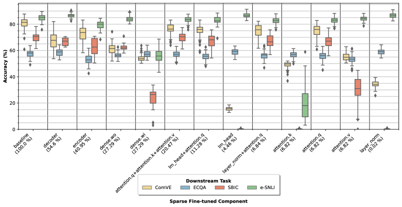
Figure 1: Distribution of the accuracy scores for different SparseFit configurations for T5-large. The percentage of parameters fine-tuned for each configuration is shown between brackets.

We present in Table 1 the accuracy performance for selected SparseFit settings for T5-large. As can be observed in Table 1, some SparseFit configurations with very few fine-tuned parameters can produce significantly better results than the baseline (i.e. full fine-tuning). For instance, fine-tuning the normalization layer ($0.02\%$ of the model’s parameters) achieves better task performance than the baseline for two out of four datasets (e-SNLI and ECQA). Furthermore, we consistently see that if two SparseFit configurations achieve good generalization results, combining them by jointly fine-tuning both components produces significantly better results than each configuration in isolation. Furthermore, we show in Figure 1 the spread of the task performance for SparseFit configurations. For all the box plots, the $x$-axis shows the different SparseFit configurations, with the percentage of fine-tuned parameters between brackets. Notice that we evaluated SparseFit on T5-base, T5-large and T5-3b, but Table 1 and Figure 1 only include the results for T5-large. We include in Appendix B the task performance for all model sizes. We found that the task accuracy is consistently higher for the largest LMs for all datasets, but the gap between T5-large and T5-3b is small ($<7\%$) compared with the increase in trainable parameters.

NLE Quality

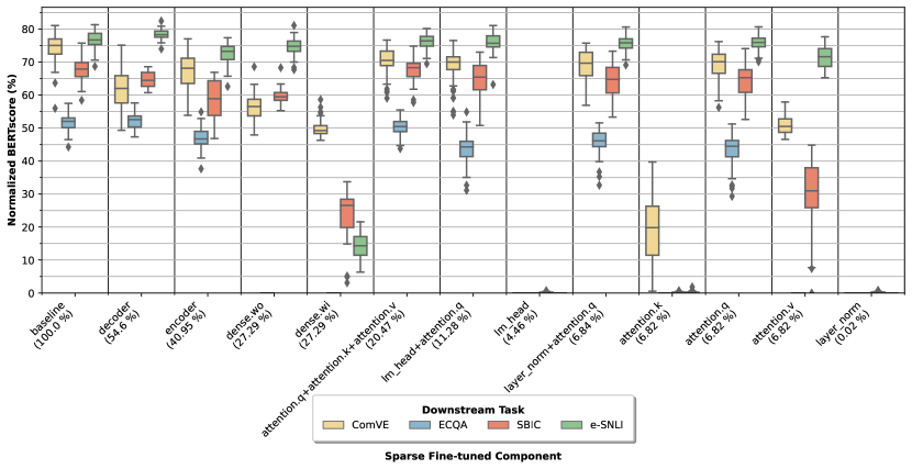
Figure 2: Distribution of the normalized BERTScore for different SparseFit settings of sparse fine-tuning for T5-large. The percentage of fine-tuned parameters is shown between brackets.

Recall that the LM is fine-tuned to conditionally generate a text in the form of “[label] because [explanation]”. Figure 2 shows the normalized BERTScore for selected SparseFit settings as a proxy to evaluate how good the NLEs generated after the explanation token (i.e. “because”) is. We can see that the best quality of NLEs is achieved for SparseFit combinations of two or more types of components (e.g. Layer Norm plus Self-attention Query). Overall, it can be observed that SparseFit settings with few trainable parameters (<$10\%$), such as the Self-attention Query, Language Model Head + Attention Query, and Layer Norm + Attention Query, are competitive with the baseline for all datasets. We also see that fine-tuning the decoder block (${\sim}54\%$ of the parameters) achieves better performance than the SOTA for two out of four datasets (e-SNLI and ECQA). The performance gap between most of the SparseFit configurations and the baseline does not exceed $15\%$ for all the datasets, even for very sparse fine-tuning strategies.

Figure 3: Example of annotator perceptual disagreement in our study for the ECQA dataset.

Unexpectedly, many SparseFit configurations that have high task accuracy (e.g. Normalization Layer) have a normalized BERTScore close or equal to zero. This happens because either the conditional generation ends the sentence after the generated label token or the explanation token (i.e. “because”) is not successfully generated. A more detailed analysis is available in Section 4.2.3. We summarize our results on NLEs quality for T5-large in Table 1. Furthermore, we show the results for other model sizes (i.e. T5-base, T5-large and T5-3b) in Section B.1. There it can be seen that the normalized BERTScore consistently increases with the size of the LM. Remarkably, the best SparseFit configurations for T5-large also achieve the best performance when fine-tuning T5-base, but they are slightly different for T5-3b.

Figure 4: Examples of generated NLEs for e-SNLI (Green), ECQA (Blue), SBIC (Red), and ComVE (Yellow).

Other PEFT Baselines

To compare SparseFit with other PEFT baselines, we also implemented LoRA Hu et al. (2022) for NLEs. Table 2 shows the downstream performance and the NLEs quality for different PEFT strategies on T5-large. It can be seen that, on average, SparseFit outperforms the other PEFT strategy. The best PEFT approach is LoRA with a performance roughly 10% lower than SparseFit. Furthermore, the quality of NLEs is considerably better for SparseFit for 3 out of 4 datasets.

		ComVE	ECQA	SBIC	e-SNLI	Avg
SparseFit LayerNorm + AttQ	Acc.	74.86 $\pm 5.27$ $\triangledown$	55.81 $\pm 3.12$ $\triangledown$	66.99 $\pm 4.4$ $\triangledown$	82.62 $\pm 2.73$ $\triangledown$	70.07 $\pm 3.88$
	nBERTs	69.02 $\pm 4.83$ $\triangledown$	45.88 $\pm 3.72$ $\triangledown$	64.29 $\pm 4.7$ $\triangledown$	75.63 $\pm 2.51$ $\triangledown$	63.7 $\pm 3.94$
LoRA	Acc.	67.7 $\pm 3.4$ $\triangledown$	39.9 $\pm 3.96$ $\triangledown$	63.32 $\pm 3.37$ $\triangledown$	84.12 $\pm 1.8$	63.76 $\pm 3.13$
	nBERTs	61.28 $\pm 3.12$ $\triangledown$	1.61 $\pm 1.55$ $\triangledown$	60.9 $\pm 3.3$ $\triangledown$	76.38 $\pm 1.65$	50.04 $\pm 2.4$

Table 2: Performance comparison between SparseFit and other PEFT strategies. We report the average and the standard deviation over the 60 few-shot train-validation splits for the accuracy metric and the normalized BERTScore (nBERTs). We show in bold the setting with the highest metric for each dataset. Significance testing was assessed via mean t-test in comparison with the baseline: $\triangledown$ represents a p-value lower than $10^{-2}$.

Human Evaluation

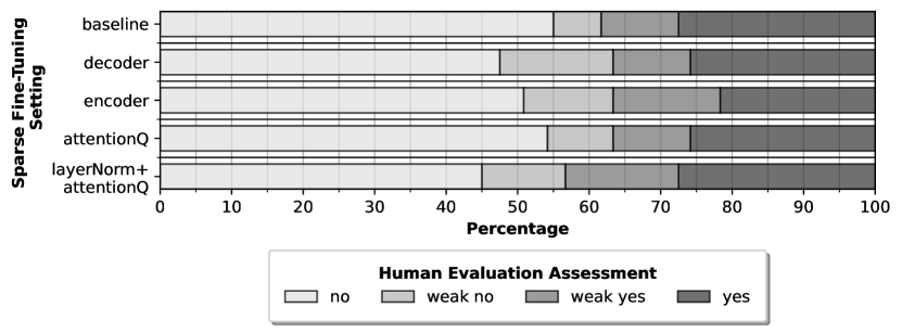
Figure 5: Illustration of plausibility score given by human annotators to quality of the NLEs generated by different SparseFit configurations. The annotators were asked to answer the question: “Does the explanation justify the answer?

We show in Figure 5 the distributions of the scores given by the human annotators for the quality of the generated NLEs, broken down for each of the best SparseFit strategies. It can be observed that approx. half of the NLEs do not justify the answer, no matter what fine-tuning strategy was used. Similarly, the proportion of NLEs that justify the prediction is close to $25\%$ regardless of the model.

The human evaluation shows that the generated NLEs are often insufficient to explain the predictions accurately. Only roughly 25% of the NLEs fully satisfy the requirement of a human evaluator. We detail the shortcomings and limitations of generated NLEs in Section 4.2. Table 3 shows a summary of the aggregated performance after remapping the plausibility scores to numerical values for different SparseFit configurations. We compute the inter-annotator agreement score using the Cohen’ $\kappa$ metric (Cohen, 1960), which is suitable for our setting since we only have two annotators evaluating the same examples.

Human Evaluation
SparseFit	e-SNLI	ECQA	SBIC	ComVE	Avg
baseline	29.63 ($0.43$)	41.92 ($0.23$)	54.44 ($0.7$)	21.67 ($0.22$)	36.91
decoder	22.22 ($0.45$)	49.49 ($0.31$)	60.0 ($0.58$)	15.56 ($0.21$)	36.82
encoder	19.14 ($0.24$)	43.43 ($0.22$)	56.67 ($0.94$)	28.33 ($0.3$)	36.89
LN+attQ	38.27 ($0.34$)	31.31 ($0.26$)	58.89 ($0.69$)	40.00 ($0.25$)	42.12
attentionQ	17.28 ($0.38$)	35.35 ($0.31$)	61.11 ($0.77$)	28.89 ($0.35$)	35.66

Table 3: Summary of the NLE quality scores given by human annotators for the best performing SparseFit configurations after mapping the human evaluation to numerical scores. The best results are in bold. In brackets, we show the inter-annotator agreement score. LN and attQ stand for LayerNorm and Self-attention Query, respectively.

4.2 Discussion

Analysis of the Generated NLEs

We show a collection of examples of the generated NLEs by the baseline and the best performing SparseFit configurations for all datasets in Figure 4. As in previous works (Camburu et al., 2018; Kayser et al., 2021; Marasovic et al., 2022), we only show examples where the label was correctly predicted by the model since we do not expect a model that predicted a wrong label to generate a correct explanation. We present in Section A.1 a more extensive list of generated NLEs with SparseFit.

4.2.1 NLE Shortcomings

Figure 6 depicts the histogram of frequencies of the shortcomings for the baseline and the best-performing SparseFit strategies. Overall, it can be observed that the most common shortcomings are Lack of explanation, Nonsensical, and Incomplete explanation. Remarkably, different SparseFit settings produce different distributions over the shortcomings. Concerning the shortcomings of the SparseFit configuration with the best generalization properties (i.e. LayerNorm + AttentionQ), the Incomplete explanation is the reason with the most occurrences, followed closely by Lack of explanation. We show a breakdown of the shortcomings for each dataset in Section B.3.

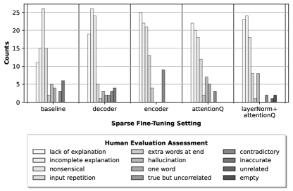
Figure 6: Histogram of the shortcomings of the generated NLEs for the baseline and the performing SparseFit configurations aggregated for all the datasets.

Figure 7: Example of annotator expectation disagreement in our study for the ECQA dataset.

4.2.2 Inter-Annotator Agreement

As shown in Table 3, the agreement between annotators is moderately low for the set of evaluated NLEs. More precisely, the annotators gave different scores to 181 out of 600 NLEs. The dataset with the most significant difference is ECQA, with 63 differences, while the SBIC dataset is the most uniform, with 17 differences. The variation between annotators can result from three potential perceptual reasons  Bourke (2014); Niño (2009). The first reason is the difference in interpretation of scores within the spectrum of possible answers (i.e. No, Weak No, Weak Yes, Yes). This means that annotators could not objectively identify the difference between a Weak Yes and a Weak No assessment. It could also happen that the annotators do not have a clear difference between a No and a Weak No score or between a Yes and a Weak Yes score. Choosing between these options could be ambiguous for the annotators, given the different perceptions about the completeness or failure of a particular explanation. To better understand this phenomenon, we show in Figure 3 an example where the annotators assigned the same (or similar) plausibility reason but a different score.

The second reason is positionality (Bourke, 2014). Positionality disagreement refers to the differences in the positions of the annotators due to their race, gender, and other socioeconomic identity factors that can alter the way they perceive the outcomes of the algorithm. This is particularly crucial for the SBIC dataset, as it contains offensive content. The third reason is related to the expectations about the quality of the generated NLEs Niño (2009). See Figure 7 for an example. In this regard, an annotator may be more strict on the characteristics that make an explanation complete and accurate.

4.2.3 Generation of Empty NLEs

As mentioned earlier, some SparseFit configurations (e.g. Layer Normalization) have high task performance but generate empty NLEs most of the time. This phenomenon can be mainly observed in the results for e-SNLI and ECQA. One possible explanation for the discrepancy between the high task accuracy and the low NLE quality is that generating NLEs is an intrinsically more complex problem than solving the downstream tasks, where the former may require fine-tuning more significant portions of the model parameters. Another explanation can be found by analyzing the pre-training tasks of the PLM and observing that, in the pre-training stage, T5 was trained on the MNLI dataset Williams et al. (2018), which is composed of NLI instances without NLEs. The weights in T5 were pre-trained on MNLI by casting the NLI task as a sequence transduction problem, where the input is a hypothesis-premise pair, and the output is the label: when only a small subset of parameters is updated (e.g. $0.02\%$ for the Layer Normalization), the model elicits its original behavior and predicts the label with high accuracy but skips the generation of the NLE. Similar reasoning may be concluded for ECQA since UnifiedQA was pre-trained on CommonsenseQA/CQA (Talmor et al., 2019), which is composed of samples with only the answer for the multiple-choice question.

5 Summary and Outlook

In this work, we introduced SparseFit, a strategy that combines sparse fine-tuning with prompt-based learning to train NLE models in a few-shot setup. SparseFit shows consistently competitive performance while only updating the Self-attention Query plus Layer Normalization, which account for ${\sim}6.8\%$ of the model parameters. The Decoder and the Self-attention Layer are also consistently among the three best performers. We also found that the sparse fine-tuning of T5-large consistently achieves better performance than fine-tuning T5-base and is slightly worse ($<5\%$) than T5-3b, no matter the SparseFit strategy. Remarkably, the top three best performers for T5-base are achieved by the same set of SparseFit configurations found for T5-large.

We aim for SparseFit to inspire the community to investigate sparse fine-tuning at different components in a model. Future work may also build upon SparseFit by, e.g. relying on soft prompts rather than hard prompts.

Limitations

Although generating natural language explanations is a fervid research area, there is still no guarantee that such explanations accurately reflect how the model works internally Wiegreffe et al. (2021); Camburu et al. (2020). For example, the fact that the generated explanation seems reasonable does not mean that the model does not rely on protected attributes and spurious correlations in the training data to produce its predictions. As such, we still recommend being careful to use self-explanatory models in production, as they can capture potentially harmful biases from the training data, even though these are not mentioned in the explanations.

Appendix A SparseFit Graphical Representation

In this paper, we propose an efficient few-shot prompt-based training regime for models generating both predictions and NLEs on top of the T5 language model. In order to have a better understanding of the active trainable parameters in each SparseFit configuration, we illustrate in Figure 8 a graphical representation of the T5 architecture with active parameters colored for the Layer Normalization sparse fine-tuning. After freezing the rest of the model (gray-colored layers), the percentage of parameters that could potentially be updated in the Layer Normalization is $0.02\%$ of the entire model. Considering that the UnifiedQA model’s architecture is the same as the one in T5, the interpretation of active parameters holds for UnifiedQA.

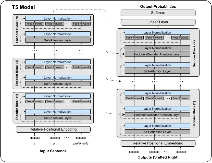
Figure 8: Illustration of the active trainable parameters in T5 when SparseFit is performed over the layer normalization.

A.1 Examples of Generated NLEs

This section shows a collection of examples of the generated NLEs by the baseline and the different sparse fine-tuning strategies considered in our approach. We show four examples for each dataset. Each example contains the generated NLE for the best performing SparseFit configurations. As in previous works (Camburu et al., 2018; Kayser et al., 2021; Marasovic et al., 2022), we only show examples where the label was correctly predicted by the model (since we do not expect a model that predicted a wrong label to generate a correct NLE). Regarding the protocol to choose the examples shown in this section, we have done a manual inspection of several possible examples, and we have chosen the more informative ones to conclude the strengths and the weaknesses of the generated NLEs. Notice that, due to the few-shot splits protocol (60 different train-validation splits), a single example could be predicted more than once for a single setup (i.e., the sample is in more than one validation set).

Figure 9: Examples of generated NLEs for e-SNLI.

Figure 10: Examples of generated NLEs for ECQA.

Figure 11: Examples of generated NLEs for SBIC.

Figure 12: Examples of generated NLEs for ComVE.

Appendix B SparseFit Full Results

This section shows the results in terms of task accuracy, and NLEs quality all configurations of SparseFit and for different model sizes (i.e. T5-base, T5-large and T5-3b). For each metric, we also break down the results by dataset.

B.1 Task Performance

Figure 1 depicts the distribution of the accuracy score for SparseFit configurations trained on top of T5-large. It can be observed that several SparseFit configurations exhibit similar performance as the baseline, particularly for ECQA and E-SNLI. The SparseFit configurations with the best task performance are Decoder, Self-Attention KQV, Self-attention Query, and Layer Normalization. Remarkably, the SparseFit configurations do not show a higher variance than the baseline across the 60 train-validation splits (inter-quartile range). Figure 13 depicts the distribution of the accuracy score for SparseFit configurations trained on top of T5-3b. It can be observed that all SparseFit configurations outperform the baseline. However, the best performance for T5-3b is achieved by the sparse fine-tuning of the Self-attention Value Layer. The results for T5-base can be observed in the breakdown done for each dataset.

Figure 13: Distribution of the accuracy scores for different SparseFit configurations for T5-3b. The percentage of parameters fine-tuned for each configuration is shown between brackets.

Figure 14 depicts the box plot with the distribution of the accuracy scores on e-SNLI for the 60 train-validation splits for different SparseFit configurations and the two pre-trained LM sizes. Overall, for e-SNLI, the task performance increases with the size of the model for most of the sparse fine-tuning configurations. Moreover, the interquartile range is considerably smaller when the model size increases (i.e., T5-large scores are less spread than the ones for T5-base). The highest median score was achieved by the fine-tuning of the Layer Normalization in T5-large, followed very closely by the fine-tuning of the LM head and the Decoder in T5-large. The combination of components (i.e. Layer Norm + Self-attention Query) performed very closely to the best-performing settings.

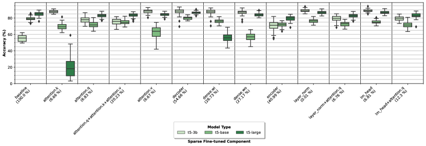
Figure 14: Distribution of the accuracies for different settings of SparseFit for the e-SNLI dataset. For each model, the variation represents the overall performance in each of the 60 train-validation splits. The percentage of parameters fine-tuned for each setup is depicted in brackets below the name of each configuration.

For the ECQA dataset, Figure 15 shows the box plot with the accuracy scores for different SparseFit setups. It can be observed that the performance of the larger LM (i.e., T5-large) is consistently better than T5-base. Overall, the accuracy is fairly similar for all the SparseFit configurations for a given LM size, with an average of $58\%$ and $42\%$ for T5-large and T5-base, respectively. Note that the random guess accuracy is $20\%$ for the ECQA dataset, since there are 5 possible answer choices. The highest accuracy was achieved by the fine-tuning of the Decoder in T5-large, followed very closely by the fine-tuning of the Layer Normalization and LM Head. The combination of components achieves a slightly lower performance than single components for the task prediction. Surprisingly, for ECQA, the variability for a given combination of configuration-model (i.e. each box) is higher for T5-large than for T5-base. Moreover, the fine-tuning of the Encoder for T5-base gives worse results in comparison with all the other configurations. Besides the setting where only the Encoder is fine-tuned for T5-base, the highest observed range in ECQA is roughly $14\%$.

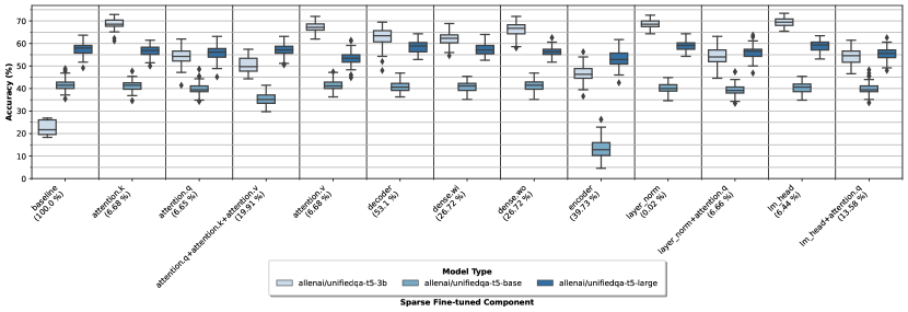
Figure 15: Distribution of the accuracy scores for different SparseFit settings for the ECQA dataset. For each model, the variation represents the overall performance in each of the 60 train-validation splits. The percentage of parameters fine-tuned for each setup is depicted in brackets below the name of each configuration.todoUpdate plot with t5-3b results

For the SBIC dataset, Figure 16 depicts the box-plot with the dispersion of accuracy scores for T5-base and T5-large. Recall that for the SBIC dataset, we fine-tune the UnifiedQA variant of T5. In general, it can be seen that the accuracy score surges when the model size is increased; thus, the best accuracy scores for a given sparse fine-tuning setup are found for the T5-large. The best median accuracy performance is achieved by the baseline. However, the difference in the median scores between the best and the second and third best-ranked configurations (i.e. Self-attention Layer and Layer Normalization + Self-attention Query, respectively) are less than $3\%$. The maximum variance among scores for the 3 best-performing SparseFit configurations is roughly $15\%$. Furthermore, it can be observed that for many sparse fine-tuning configurations, the accuracy score is close to or equal to zero. Even though the performance of a random model is $50\%$, an accuracy of $0\%$ is feasible in our scenario as the model could generate different words from the ones expected as labels. In this regard, the accuracy scores of zero are a consequence of the fact that, after the conditional generation, the model generates neither “offensive" nor “non-offensive" for any sample in the validation set. Notice that this phenomenon is particularly happening when only a small fraction of weights is fine-tuned.

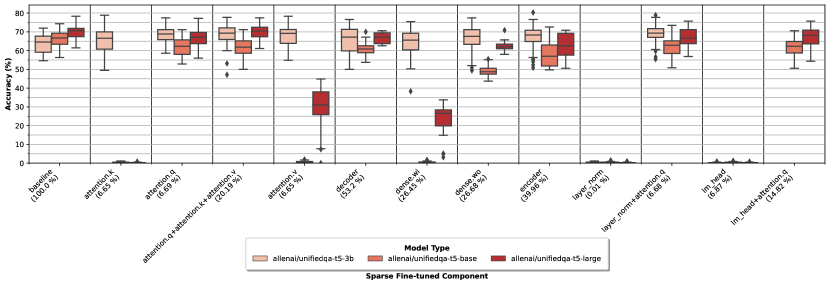
Figure 16: Distribution of the accuracy scores for different settings of SparseFit for the SBIC dataset. For each model, the variation represents the overall performance in each of the 60 train-validation splits. The percentage of parameters fine-tuned for each setup is depicted in brackets below the name of each configuration.

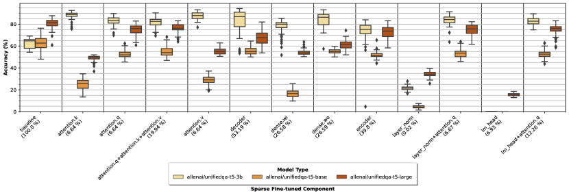
Figure 17: Distribution of the accuracy scores for different settings of SparseFit for the ComVE dataset. For each model, the variation represents the overall performance in each of the 60 train-validation splits. The percentage of parameters fine-tuned for each setup is depicted in brackets below the name of each configuration.

For the ComVE dataset, we show in Figure 17 the accuracy for the 60 different train-validation splits for different SparseFit settings and model sizes. It can be seen that the best-performing setting in terms of accuracy is the baseline for UNIFIEDQA-T5-large. (i.e. Self-attention Layer and Layer Normalization + Self-attention Query fine-tuning are the second and third best performing, respectively. Overall, the fine-tuning of the Normalization Layer leads to the worst task performance. Moreover, it can be observed that the performance increases with the size of the model, thus UNIFIEDQA-T5-large always performs better than UNIFIEDQA-T5-base for all the fine-tuning configurations. The smallest gap in performance between model sizes (UNIFIEDQA-T5-large vs. UNIFIEDQA-T5-base) happens for the fine-tuning of the Dense Layer. Conversely, the maximum spread in performance (i.e. the difference between the best and the worst split) is around $21\%$ for models trained using the UNIFIEDQA-T5-large architecture.

B.2 Explanation Generation Performance

Figure 2 shows the box-plot with the normalized BERTscores for different SparseFit setups fine-tuned on top of T5-large. In addition to explained in the main text, it can be seen that combinations of components lead to less variance in the score achieved for the 60 train-test splits (see the interquartile range). Furthermore, Table 4 shows the performance summary for the downstream performance and the NLEs quality for T5-3b. It can be observed that the Attention Value Layer achieves the best performance on average. We highlight that SparseFit outperforms the baseline (i.e. full fine-tuning) for all datasets.

SparseFit		ComVE	ECQA	SBIC	e-SNLI	Avg
Baseline ($100.00\%$)	Acc.	62.48 $\pm 6.03$	22.39 $\pm 3.61$	63.55 $\pm 6.59$	55.3 $\pm 4.98$	50.93 $\pm 5.3$
	nBERTs	55.55 $\pm 5.6$	19.73 $\pm 3.22$	61.21 $\pm 6.79$	49.25 $\pm 4.36$	46.44 $\pm 4.99$
Decoder ($54.60\%$)	Acc.	83.67 $\pm 10.12$ $\triangledown$	62.62 $\pm 4.16$ $\triangledown$	65.59 $\pm 7.51$	87.48 $\pm 4.02$ $\triangledown$	74.84 $\pm 6.45$
	nBERTs	74.66 $\pm 9.02$ $\triangledown$	55.31 $\pm 3.65$ $\triangledown$	62.72 $\pm 7.66$	77.92 $\pm 3.7$ $\triangledown$	67.65 $\pm 6.01$
Encoder ($40.95\%$)	Acc.	73.14 $\pm 11.24$ $\triangledown$	46.23 $\pm 3.96$ $\triangledown$	66.81 $\pm 6.43$	70.34 $\pm 5.79$ $\triangledown$	64.13 $\pm 6.86$
	nBERTs	66.7 $\pm 10.28$ $\triangledown$	41.46 $\pm 3.56$ $\triangledown$	64.45 $\pm 6.7$	63.79 $\pm 5.28$ $\triangledown$	59.1 $\pm 6.46$
Dense.wo ($27.29\%$)	Acc.	83.91 $\pm 6.54$ $\triangledown$	66.21 $\pm 3.12$ $\triangledown$	66.64 $\pm 6.46$	86.85 $\pm 3.0$ $\triangledown$	75.9 $\pm 4.78$
	nBERTs	76.1 $\pm 6.04$ $\triangledown$	59.12 $\pm 2.76$ $\triangledown$	63.87 $\pm 6.51$	78.24 $\pm 2.78$ $\triangledown$	69.33 $\pm 4.52$
Dense.wi ($27.29\%$)	Acc.	77.6 $\pm 6.63$ $\triangledown$	62.12 $\pm 2.75$ $\triangledown$	63.99 $\pm 7.4$	87.31 $\pm 3.6$ $\triangledown$	72.76 $\pm 5.1$
	nBERTs	70.21 $\pm 6.04$ $\triangledown$	55.12 $\pm 2.44$ $\triangledown$	61.05 $\pm 7.43$	78.24 $\pm 3.28$ $\triangledown$	66.16 $\pm 4.8$
Attention KQV ($20.47\%$)	Acc.	81.73 $\pm 4.14$ $\triangledown$	50.24 $\pm 3.48$ $\triangledown$	68.84 $\pm 5.37$ $\triangledown$	75.3 $\pm 3.78$ $\triangledown$	69.03 $\pm 4.19$
	nBERTs	74.27 $\pm 3.84$ $\triangledown$	44.79 $\pm 3.06$ $\triangledown$	66.12 $\pm 5.46$ $\triangledown$	67.67 $\pm 3.36$ $\triangledown$	63.21 $\pm 3.93$
LM head + Attention.Q ($11.28\%$)	Acc.	82.59 $\pm 3.37$ $\triangledown$	54.28 $\pm 3.57$ $\triangledown$	0.0 $\pm 0.0$	79.33 $\pm 2.94$ $\triangledown$	72.07 $\pm 3.29$
	nBERTs	75.2 $\pm 3.0$ $\triangledown$	48.42 $\pm 3.17$ $\triangledown$	0.0 $\pm 0.0$	71.52 $\pm 2.74$ $\triangledown$	65.05 $\pm 2.97$
LM head ($4.46\%$)	Acc.	0.09 $\pm 0.13$ $\triangledown$	69.43 $\pm 1.88$ $\triangledown$	0.23 $\pm 0.22$ $\triangledown$	89.04 $\pm 1.63$ $\triangledown$	39.7 $\pm 0.96$
	nBERTs	0.0 $\pm 0.0$ $\triangledown$	0.0 $\pm 0.0$ $\triangledown$	0.19 $\pm 0.18$ $\triangledown$	0.0 $\pm 0.0$ $\triangledown$	0.05 $\pm 0.04$
LayerNorm + Attention.Q ($6.84\%$)	Acc.	83.27 $\pm 4.52$ $\triangledown$	54.13 $\pm 3.86$ $\triangledown$	68.87 $\pm 4.86$ $\triangledown$	79.16 $\pm 3.72$ $\triangledown$	71.36 $\pm 4.24$
	nBERTs	75.83 $\pm 4.14$ $\triangledown$	48.31 $\pm 3.46$ $\triangledown$	65.86 $\pm 5.07$ $\triangledown$	71.27 $\pm 3.44$ $\triangledown$	65.32 $\pm 4.03$
Attention.Q ($6.82\%$)	Acc.	83.09 $\pm 4.15$ $\triangledown$	54.39 $\pm 3.66$ $\triangledown$	68.44 $\pm 4.44$ $\triangledown$	77.88 $\pm 3.66$ $\triangledown$	70.95 $\pm 3.98$
	nBERTs	75.65 $\pm 3.76$ $\triangledown$	48.56 $\pm 3.24$ $\triangledown$	65.4 $\pm 4.68$ $\triangledown$	70.23 $\pm 3.41$ $\triangledown$	64.96 $\pm 3.77$
Attention.K ($6.82\%$)	Acc.	87.7 $\pm 3.83$ $\triangledown$	68.74 $\pm 2.29$ $\triangledown$	65.48 $\pm 6.26$	87.8 $\pm 1.83$ $\triangledown$	77.43 $\pm 3.55$
	nBERTs	80.01 $\pm 3.52$ $\triangledown$	61.25 $\pm 2.07$ $\triangledown$	62.41 $\pm 6.5$	79.55 $\pm 1.62$ $\triangledown$	70.8 $\pm 3.43$
Attention.V ($6.82\%$)	Acc.	87.72 $\pm 3.16$ $\triangledown$	67.22 $\pm 2.14$ $\triangledown$	68.11 $\pm 5.19$ $\triangledown$	88.17 $\pm 2.38$ $\triangledown$	77.81 $\pm 3.22$
	nBERTs	79.87 $\pm 2.92$ $\triangledown$	60.12 $\pm 1.9$ $\triangledown$	65.67 $\pm 5.09$ $\triangledown$	79.63 $\pm 2.26$ $\triangledown$	71.32 $\pm 3.04$
LayerNorm ($0.02\%$)	Acc.	21.37 $\pm 2.06$ $\triangledown$	68.71 $\pm 1.89$ $\triangledown$	0.29 $\pm 0.27$ $\triangledown$	88.91 $\pm 1.74$ $\triangledown$	44.82 $\pm 1.49$
	nBERTs	0.0 $\pm 0.0$ $\triangledown$	0.0 $\pm 0.0$ $\triangledown$	0.24 $\pm 0.22$ $\triangledown$	0.0 $\pm 0.0$ $\triangledown$	0.06 $\pm 0.06$

Table 4: Summary of best performing SparseFit configurations for T5-3B. We report the average and the standard deviation over the 60 few-shot train-validation splits for the accuracy metric and the normalized BERTScore (nBERTs). In brackets are the percentages of fine-tuned weights for each SparseFit configuration. We show in bold the setting with the highest metric for each dataset. Significance testing was assessed via mean t-test in comparison with the baseline: $\triangledown$ represents a p-value lower than $10^{-2}$.

For e-SNLI, Figure 19 shows the normalized BERTscore over the 60 few-shot learning splits for different SparseFit configurations. Overall, for every sparse fine-tuning setting, the BERTscore is consistently higher for the largest PLM (i.e. T5-large). However, the gap in performance is smaller for the best-performing sparse fine-tuning configurations. For instance, the difference in the average normalized BERTscore values between T5-large and T5-base for the best performing SparseFit (i.e., Decoder) is roughly $5\%$ while for the worst performing configuration is around $68\%$. The first five best-performing SparseFit configurations for T5-large are Decoder, Baseline, Self-attention KVQ, Layer Normalization + Self-attention Q, and Self-attention Values. Note that the normalized BERTscore is zero for some sparse fine-tuning configurations (e.g., Layer Normalization). This is mostly happening when the sparse fine-tuning is applied to small models (i.e., T5-base). The fact that the BERTscore is zero for a given configuration for all the samples in a split implies that the generated NLEs are always empty. We explore the reasons behind this phenomenon in Section 4.2.3

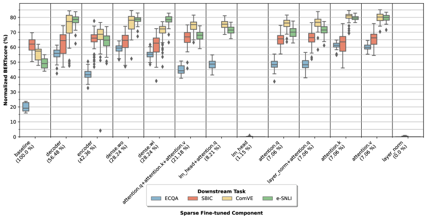
Figure 18: Distribution of the normalized BERTScore for different SparseFit settings of sparse fine-tuning for T5-3b. The percentage of fine-tuned parameters is shown between brackets.

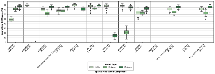
Figure 19: Distribution of the normalized BERTscore for different settings of sparse fine-tuning for the e-SNLI dataset. For each model, the box represents the overall performance over the 60 train-validation splits. The percentage of parameters fine-tuned for each setup is depicted in brackets below the name of each configuration.

For the ECQA dataset, we show in Figure 20 the spread of the normalized BERTscore for all SparseFit configurations. Without exception, the largest model (T5-large) outperforms the T5-base models for every setting. Remarkably, for ECQA, many sparse fine-tuning configurations lead to the generation of empty explanations. Particularly, only the fine-tuning of the Baseline, the Decoder, and the Encoder are able to consistently generate non-empty explanations no matter the size of the model. Among the configurations that generate non-empty explanations, the best normalized BERTscores are achieved by the Decoder sparse fine-tuning, followed by the Baseline and Encoder Blocks fine-tuning. Note that for all of these configurations, the interquartile range is smaller than $6\%$ regardless of the model size. Moreover, the fine-tuning of Self-attention Query achieves competitive results for T5-large but zero BERTscore for T5-base.

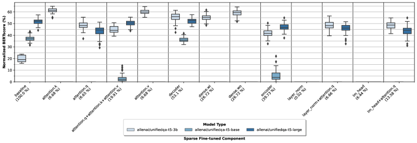
Figure 20: Distribution of the normalized BERTscore for different settings of sparse fine-tuning for the ECQA dataset. For each model, the box represents the overall performance over the 60 train-validation splits. The percentage of parameters fine-tuned for each setup is depicted in brackets below the name of each configuration.

Figure 21 shows the normalized BERTscore results for the SBIC dataset. Recall that for the SBIC dataset, we fine-tune the UnifiedQA variant of T5. As expected, the model size contributes to better performance. Consequently, the BERTscore is higher for the T5-large model for every sparse fine-tuning configuration. The best BERTscore median is achieved by the Baseline in combination with the UNIFIEDQA-T5-large, with a metric value of $\approx 68\%$. The second and third best-performing setups are the Decoder and the Encoder, respectively. Moreover, the fine-tuning of layers such as the Normalization Layer or Self-attention Layer results in the generation of text that does not contain the explanation token “because”, thus the BERTscore is close to zero for those configurations.

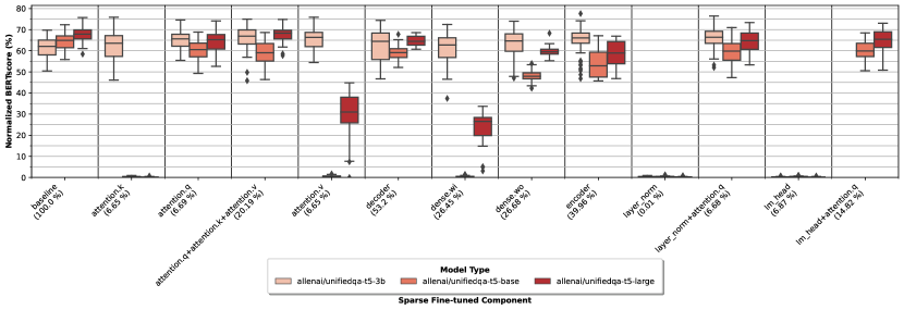
Figure 21: Distribution of the normalized BERTscore for different settings of sparse fine-tuning for the SBIC dataset. For each model, the box represents the overall performance over the 60 train-validation splits. The percentage of parameters fine-tuned for each setup is depicted in brackets below the name of each configuration.

We depict in Figure 22 the variation of the normalized BERTscore metric over the 60 different train-validation splits for the SparseFit configurations. Recall that for ComVE dataset, we fine-tune the UnifiedQA variant of T5. Overall, the BERTscore is substantially higher for T5-large. The best BERTscore for T5-large is obtained by the Baseline fine-tuning, with a median score of $75\%$ for the 60 different seeds. Similar behavior can be seen for T5-base, where Baseline is also the setting with the best explanations (from the perspective of the automatic metric). The second and third best sparse fine-tuning setups are the Self-attention Query and Baseline, respectively. Notice that the difference in the median between the Baseline and the Encoder is around $3\%$. Moreover, the variance among the different splits for a given sparse fine-tuning setting is on average higher than for the Baseline. Remarkably, the sparse fine-tuning over the Normalization Layer was the only setting that obtained a zero BERTscore for the ComVE dataset.

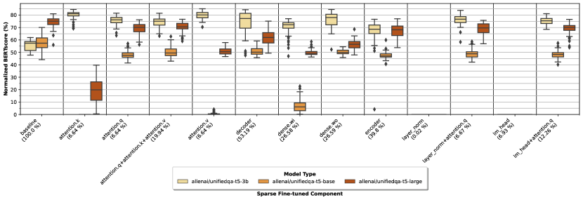
Figure 22: Distribution of the normalized BERTscore for different settings of sparse fine-tuning for the ComVE dataset. The baseline model represents the work done by Marasovic et al. (2022), where all the parameters of the LM were fine-tuned. For each model, the box represents the overall performance over the 60 train-validation splits. The percentage of parameters fine-tuned for each setup is depicted in brackets below the name of each configuration.

B.3 Explanations Shortcomings per Dataset

Given the diverse nature of the studied datasets, we perform an individual analysis for each dataset in order to find the particular deficiencies and traits of the explanations by dataset. Figure 24 shows a set of histograms with the assessment of the annotators on shortcomings for the e-SNLI dataset. It can be seen that the Nonsensical category is consistently the most common no matter what fine-tuning strategy was used. Below, the reader can find two examples of Nonsensical explanations generated by the Baseline and the Decoder strategy, respectively.

Figure 23: Examples of Non-sensical NLEs generated for e-SNLI.

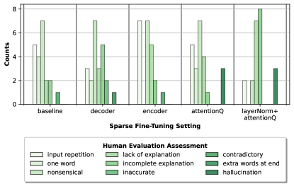
Figure 24: Histogram of the occurrences of the main shortcomings of the generated explanations for the baseline and the two best performing sparse fine-tuning setup for the e-SNLI dataset.

In addition to this, Input Repetition is the second most common shortcoming for e-SNLI. A regular pattern found in the generated explanations is the repetition of a sub-string of the hypothesis as the predicted explanation, which happens for around $17\%$ of the generated explanations. Below, the reader can see an example of input repetition found in the e-SNLI dataset.

Figure 25: Examples of Input-Repetition NLEs generated for e-SNLI.

We depict in Figure 27 a set of histograms with the number of times that a shortcoming category happens for different fine-tuning strategies for ECQA. Predominantly, Incomplete Explanation is the main weakness of generated NLEs. Notice that for this dataset, the answers are not generally shared by different samples (i.e., the possible labels for a sample are not always the same as in the other datasets). This causes the generated explanations to be vague and incomplete. Below, the reader can see 3 examples of Incomplete Explanation generated by the Baseline, Decoder, and Encoder fine-tuning strategy, respectively.

Figure 26: Examples of Incomplete Explanation NLEs generated for ECQA.

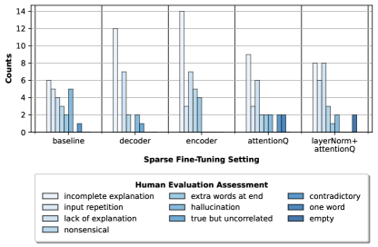
Figure 27: Histogram of the occurrences of the main shortcomings of the generated explanations for the baseline and the two best performing sparse fine-tuning setup for the ECQA dataset.

Figure 29 shows a set of histograms with the assessment done by the annotators about the most common shortcomings. Different from other datasets, there is no singular shortcoming that dominates the results for all the fine-tuning setups. The most common mistakes among all the explanations in the dataset are: Inaccurate, Nonsensical, and Incomplete Explanation. Below, the reader can find an example for the Incomplete Explanation shortcoming for the Decoder fine-tuning.

Figure 28: Examples of Incomplete Explanation NLEs generated for SBIC.

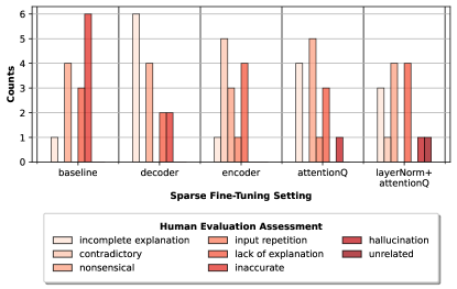
Figure 29: Histogram of the occurrences of the most common explanation shortcomings for the baseline and the two best performing sparse fine-tuning setup for the SBIC dataset.

We have depicted in Figure 30 a series of histograms with the frequency of possible shortcomings given by human annotators to the evaluated explanations. It can be seen that annotators consider that the Lack of explanation, Nonsensical, and Incomplete Explanation are the most relevant categories to explain the weaknesses of the generated explanations.

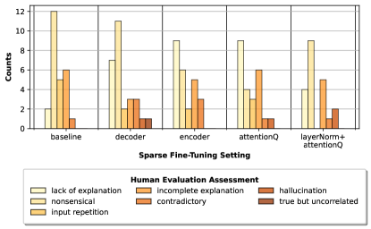
Figure 30: Histogram of the occurrences of the most common explanation shortcomings for the baseline and the two best performing sparse fine-tuning setup for the ComVE dataset.

References

- Aggarwal et al. (2021) Shourya Aggarwal, Divyanshu Mandowara, Vishwajeet Agrawal, Dinesh Khandelwal, Parag Singla, and Dinesh Garg. 2021. Explanations for commonsenseqa: New dataset and models. In Workshop on Commonsense Reasoning and Knowledge Bases.
- Akula et al. (2020) Arjun R. Akula, Shuai Wang, and Song-Chun Zhu. 2020. Cocox: Generating conceptual and counterfactual explanations via fault-lines. In AAAI, pages 2594–2601. AAAI Press.
- Alaa and van der Schaar (2019) Ahmed M. Alaa and Mihaela van der Schaar. 2019. Demystifying black-box models with symbolic metamodels. In NeurIPS, pages 11301–11311.
- Ba et al. (2016) Lei Jimmy Ba, Jamie Ryan Kiros, and Geoffrey E. Hinton. 2016. Layer normalization. CoRR, abs/1607.06450.
- Barham et al. (2022) Paul Barham, Aakanksha Chowdhery, Jeff Dean, Sanjay Ghemawat, Steven Hand, Dan Hurt, Michael Isard, Hyeontaek Lim, Ruoming Pang, Sudip Roy, Brennan Saeta, Parker Schuh, Ryan Sepassi, Laurent El Shafey, Chandramohan A. Thekkath, and Yonghui Wu. 2022. Pathways: Asynchronous distributed dataflow for ML. In MLSys. mlsys.org.
- Bourke (2014) Brian Bourke. 2014. Positionality: Reflecting on the research process. The qualitative report, 19(33):1–9.
- Brock et al. (2018) Andrew Brock, Theo Lim, JM Ritchie, and Nick Weston. 2018. Smash: One-shot model architecture search through hypernetworks. In International Conference on Learning Representations.
- Brown et al. (2020) Tom Brown, Benjamin Mann, Nick Ryder, Melanie Subbiah, Jared D Kaplan, Prafulla Dhariwal, Arvind Neelakantan, Pranav Shyam, Girish Sastry, Amanda Askell, Sandhini Agarwal, Ariel Herbert-Voss, Gretchen Krueger, Tom Henighan, Rewon Child, Aditya Ramesh, Daniel Ziegler, Jeffrey Wu, Clemens Winter, Chris Hesse, Mark Chen, Eric Sigler, Mateusz Litwin, Scott Gray, Benjamin Chess, Jack Clark, Christopher Berner, Sam McCandlish, Alec Radford, Ilya Sutskever, and Dario Amodei. 2020. Language models are few-shot learners. In Advances in Neural Information Processing Systems, volume 33, pages 1877–1901. Curran Associates, Inc.
- Camburu et al. (2021) Oana-Maria Camburu, Eleonora Giunchiglia, Jakob Foerster, Thomas Lukasiewicz, and Phil Blunsom. 2021. The struggles of feature-based explanations: Shapley values vs. minimal sufficient subsets. In AAAI 2021 Workshop on Explainable Agency in Artificial Intelligence.
- Camburu et al. (2018) Oana-Maria Camburu, Tim Rocktäschel, Thomas Lukasiewicz, and Phil Blunsom. 2018. e-SNLI: Natural language inference with natural language explanations. Advances in Neural Information Processing Systems, 31.
- Camburu et al. (2020) Oana-Maria Camburu, Brendan Shillingford, Pasquale Minervini, Thomas Lukasiewicz, and Phil Blunsom. 2020. Make up your mind! adversarial generation of inconsistent natural language explanations. In ACL, pages 4157–4165. Association for Computational Linguistics.
- Chen et al. (2021) Hanxiong Chen, Xu Chen, Shaoyun Shi, and Yongfeng Zhang. 2021. Generate natural language explanations for recommendation. CoRR, abs/2101.03392.
- Chowdhery et al. (2022) Aakanksha Chowdhery, Sharan Narang, Jacob Devlin, Maarten Bosma, Gaurav Mishra, Adam Roberts, Paul Barham, Hyung Won Chung, Charles Sutton, Sebastian Gehrmann, Parker Schuh, Kensen Shi, Sasha Tsvyashchenko, Joshua Maynez, Abhishek Rao, Parker Barnes, Yi Tay, Noam Shazeer, Vinodkumar Prabhakaran, Emily Reif, Nan Du, Ben Hutchinson, Reiner Pope, James Bradbury, Jacob Austin, Michael Isard, Guy Gur-Ari, Pengcheng Yin, Toju Duke, Anselm Levskaya, Sanjay Ghemawat, Sunipa Dev, Henryk Michalewski, Xavier Garcia, Vedant Misra, Kevin Robinson, Liam Fedus, Denny Zhou, Daphne Ippolito, David Luan, Hyeontaek Lim, Barret Zoph, Alexander Spiridonov, Ryan Sepassi, David Dohan, Shivani Agrawal, Mark Omernick, Andrew M. Dai, Thanumalayan Sankaranarayana Pillai, Marie Pellat, Aitor Lewkowycz, Erica Moreira, Rewon Child, Oleksandr Polozov, Katherine Lee, Zongwei Zhou, Xuezhi Wang, Brennan Saeta, Mark Diaz, Orhan Firat, Michele Catasta, Jason Wei, Kathy Meier-Hellstern, Douglas Eck, Jeff Dean, Slav Petrov, and Noah Fiedel. 2022. Palm: Scaling language modeling with pathways. CoRR, abs/2204.02311.
- Cohen (1960) Jacob Cohen. 1960. A coefficient of agreement for nominal scales. Educational and Psychological Measurement, 20(1):37–46.
- Devlin et al. (2019) Jacob Devlin, Ming-Wei Chang, Kenton Lee, and Kristina Toutanova. 2019. BERT: pre-training of deep bidirectional transformers for language understanding. In NAACL-HLT (1), pages 4171–4186. Association for Computational Linguistics.
- Dong et al. (2019) Li Dong, Nan Yang, Wenhui Wang, Furu Wei, Xiaodong Liu, Yu Wang, Jianfeng Gao, Ming Zhou, and Hsiao-Wuen Hon. 2019. Unified language model pre-training for natural language understanding and generation. Advances in Neural Information Processing Systems, 32.
- Dong et al. (2018) Xuanyi Dong, Linchao Zhu, De Zhang, Yi Yang, and Fei Wu. 2018. Fast parameter adaptation for few-shot image captioning and visual question answering. In Proceedings of the 26th ACM international conference on Multimedia, pages 54–62.
- Ehsan et al. (2018) Upol Ehsan, Brent Harrison, Larry Chan, and Mark O Riedl. 2018. Rationalization: A neural machine translation approach to generating natural language explanations. In Proceedings of the 2018 AAAI/ACM Conference on AI, Ethics, and Society, pages 81–87.
- Finn et al. (2017) Chelsea Finn, Pieter Abbeel, and Sergey Levine. 2017. Model-agnostic meta-learning for fast adaptation of deep networks. In ICML, volume 70 of Proceedings of Machine Learning Research, pages 1126–1135. PMLR.
- Hendricks et al. (2018) Lisa Anne Hendricks, Ronghang Hu, Trevor Darrell, and Zeynep Akata. 2018. Grounding visual explanations. In Proceedings of the European Conference on Computer Vision (ECCV).
- Houlsby et al. (2019) Neil Houlsby, Andrei Giurgiu, Stanislaw Jastrzebski, Bruna Morrone, Quentin de Laroussilhe, Andrea Gesmundo, Mona Attariyan, and Sylvain Gelly. 2019. Parameter-efficient transfer learning for NLP. In ICML, volume 97 of Proceedings of Machine Learning Research, pages 2790–2799. PMLR.
- Hu et al. (2022) Edward J Hu, yelong shen, Phillip Wallis, Zeyuan Allen-Zhu, Yuanzhi Li, Shean Wang, Lu Wang, and Weizhu Chen. 2022. LoRA: Low-rank adaptation of large language models. In International Conference on Learning Representations.
- IV et al. (2022) Robert L. Logan IV, Ivana Balazevic, Eric Wallace, Fabio Petroni, Sameer Singh, and Sebastian Riedel. 2022. Cutting down on prompts and parameters: Simple few-shot learning with language models. In ACL (Findings), pages 2824–2835. Association for Computational Linguistics.
- Izacard et al. (2022) Gautier Izacard, Patrick S. H. Lewis, Maria Lomeli, Lucas Hosseini, Fabio Petroni, Timo Schick, Jane Dwivedi-Yu, Armand Joulin, Sebastian Riedel, and Edouard Grave. 2022. Few-shot learning with retrieval augmented language models. CoRR, abs/2208.03299.
- Kaur et al. (2020) Harmanpreet Kaur, Harsha Nori, Samuel Jenkins, Rich Caruana, Hanna Wallach, and Jennifer Wortman Vaughan. 2020. Interpreting interpretability: Understanding data scientists’ use of interpretability tools for machine learning. In Proceedings of the CHI Conference on Human Factors in Computing Systems.
- Kayser et al. (2021) Maxime Kayser, Oana-Maria Camburu, Leonard Salewski, Cornelius Emde, Virginie Do, Zeynep Akata, and Thomas Lukasiewicz. 2021. e-ViL: A dataset and benchmark for natural language explanations in vision-language tasks. In Proceedings of the IEEE/CVF International Conference on Computer Vision, pages 1244–1254.
- Kayser et al. (2022) Maxime Kayser, Cornelius Emde, Oana-Maria Camburu, Guy Parsons, Bartlomiej Papiez, and Thomas Lukasiewicz. 2022. Explaining chest x-ray pathologies in natural language. In Medical Image Computing and Computer Assisted Intervention – MICCAI 2022, pages 701–713, Cham. Springer Nature Switzerland.
- Khashabi et al. (2020) D. Khashabi, S. Min, T. Khot, A. Sabhwaral, O. Tafjord, P. Clark, and H. Hajishirzi. 2020. Unifiedqa: Crossing format boundaries with a single qa system. EMNLP - findings.
- Kim et al. (2018) Jinkyu Kim, Anna Rohrbach, Trevor Darrell, John F. Canny, and Zeynep Akata. 2018. Textual explanations for self-driving vehicles. In ECCV (2), volume 11206 of Lecture Notes in Computer Science, pages 577–593. Springer.
- Lampert et al. (2009) Christoph H. Lampert, Hannes Nickisch, and Stefan Harmeling. 2009. Learning to detect unseen object classes by between-class attribute transfer. In CVPR, pages 951–958. IEEE Computer Society.
- Li and Liang (2021) Xiang Lisa Li and Percy Liang. 2021. Prefix-tuning: Optimizing continuous prompts for generation. In ACL/IJCNLP (1), pages 4582–4597. Association for Computational Linguistics.
- Ling et al. (2017) Wang Ling, Dani Yogatama, Chris Dyer, and Phil Blunsom. 2017. Program induction by rationale generation: Learning to solve and explain algebraic word problems. In ACL (1), pages 158–167. Association for Computational Linguistics.
- Liu et al. (2021) Pengfei Liu, Weizhe Yuan, Jinlan Fu, Zhengbao Jiang, Hiroaki Hayashi, and Graham Neubig. 2021. Pre-train, prompt, and predict: A systematic survey of prompting methods in natural language processing. arXiv preprint arXiv:2107.13586.
- Loshchilov and Hutter (2019) Ilya Loshchilov and Frank Hutter. 2019. Decoupled weight decay regularization. In 7th International Conference on Learning Representations, ICLR 2019, New Orleans, LA, USA, May 6-9, 2019. OpenReview.net.
- Lundberg and Lee (2017) Scott M. Lundberg and Su-In Lee. 2017. A unified approach to interpreting model predictions. In NIPS, pages 4765–4774.
- Majumder et al. (2022) Bodhisattwa Prasad Majumder, Oana-Maria Camburu, Thomas Lukasiewicz, and Julian Mcauley. 2022. Knowledge-grounded self-rationalization via extractive and natural language explanations. In Proceedings of the 39th International Conference on Machine Learning, volume 162 of Proceedings of Machine Learning Research, pages 14786–14801. PMLR.
- Marasovic et al. (2022) Ana Marasovic, Iz Beltagy, Doug Downey, and Matthew Peters. 2022. Few-shot self-rationalization with natural language prompts. In Findings of the Association for Computational Linguistics: NAACL 2022, pages 410–424, Seattle, United States. Association for Computational Linguistics.
- Marasović et al. (2020) Ana Marasović, Chandra Bhagavatula, Jae sung Park, Ronan Le Bras, Noah A Smith, and Yejin Choi. 2020. Natural language rationales with full-stack visual reasoning: From pixels to semantic frames to commonsense graphs. In Findings of the Association for Computational Linguistics: EMNLP 2020, pages 2810–2829.
- Narang et al. (2020) Sharan Narang, Colin Raffel, Katherine Lee, Adam Roberts, Noah Fiedel, and Karishma Malkan. 2020. Wt5?! training text-to-text models to explain their predictions. CoRR, abs/2004.14546.
- Niño (2009) Ana Niño. 2009. Machine translation in foreign language learning: Language learners’ and tutors’ perceptions of its advantages and disadvantages. ReCALL, 21(2):241–258.
- Park et al. (2018) Dong Huk Park, Lisa Anne Hendricks, Zeynep Akata, Anna Rohrbach, Bernt Schiele, Trevor Darrell, and Marcus Rohrbach. 2018. Multimodal explanations: Justifying decisions and pointing to the evidence. In Proceedings of the IEEE conference on computer vision and pattern recognition, pages 8779–8788.
- Radford et al. (2018) Alec Radford, Karthik Narasimhan, Tim Salimans, Ilya Sutskever, et al. 2018. Improving language understanding by generative pre-training.
- Raffel et al. (2020) Colin Raffel, Noam Shazeer, Adam Roberts, Katherine Lee, Sharan Narang, Michael Matena, Yanqi Zhou, Wei Li, and Peter J. Liu. 2020. Exploring the limits of transfer learning with a unified text-to-text transformer. Journal of Machine Learning Research, 21(140):1–67.
- Ren et al. (2018) Mengye Ren, Eleni Triantafillou, Sachin Ravi, Jake Snell, Kevin Swersky, Joshua B Tenenbaum, Hugo Larochelle, and Richard S Zemel. 2018. Meta-learning for semi-supervised few-shot classification. In International Conference on Learning Representations.
- Ribeiro et al. (2016) Marco Túlio Ribeiro, Sameer Singh, and Carlos Guestrin. 2016. "why should I trust you?": Explaining the predictions of any classifier. In HLT-NAACL Demos, pages 97–101. The Association for Computational Linguistics.
- Sap et al. (2020) Maarten Sap, Saadia Gabriel, Lianhui Qin, Dan Jurafsky, Noah A. Smith, and Yejin Choi. 2020. Social bias frames: Reasoning about social and power implications of language. In Proceedings of the 58th Annual Meeting of the Association for Computational Linguistics, pages 5477–5490, Online. Association for Computational Linguistics.
- Satorras and Estrach (2018) Victor Garcia Satorras and Joan Bruna Estrach. 2018. Few-shot learning with graph neural networks. In International Conference on Learning Representations.
- Schwartz et al. (2020) Roy Schwartz, Jesse Dodge, Noah A. Smith, and Oren Etzioni. 2020. Green AI. Commun. ACM, 63(12):54–63.
- Sha et al. (2021) Lei Sha, Oana-Maria Camburu, and Thomas Lukasiewicz. 2021. Learning from the best: Rationalizing prediction by adversarial information calibration. In Proceedings of the 35th Association for the Advancement of Artificial Intelligence (AAAI).
- Shrikumar et al. (2017) Avanti Shrikumar, Peyton Greenside, and Anshul Kundaje. 2017. Learning important features through propagating activation differences. In ICML, volume 70 of Proceedings of Machine Learning Research, pages 3145–3153. PMLR.
- Solano et al. (2020) Jesús Solano, Lizzy Tengana, Alejandra Castelblanco, Esteban Rivera, Christian Lopez, and Martın Ochoa. 2020. A few-shot practical behavioral biometrics model for login authentication in web applications. In NDSS Workshop on Measurements, Attacks, and Defenses for the Web (MADWeb’20).
- Talmor et al. (2019) Alon Talmor, Jonathan Herzig, Nicholas Lourie, and Jonathan Berant. 2019. CommonsenseQA: A question answering challenge targeting commonsense knowledge. In Proceedings of the 2019 Conference of the North American Chapter of the Association for Computational Linguistics: Human Language Technologies, Volume 1 (Long and Short Papers), pages 4149–4158, Minneapolis, Minnesota. Association for Computational Linguistics.
- Vinyals et al. (2016) Oriol Vinyals, Charles Blundell, Tim Lillicrap, Koray Kavukcuoglu, and Daan Wierstra. 2016. Matching networks for one shot learning. In NIPS, pages 3630–3638.
- Wallace et al. (2019) Eric Wallace, Jens Tuyls, Junlin Wang, Sanjay Subramanian, Matt Gardner, and Sameer Singh. 2019. Allennlp interpret: A framework for explaining predictions of NLP models. In EMNLP/IJCNLP (3), pages 7–12. Association for Computational Linguistics.
- Wang et al. (2019) Cunxiang Wang, Shuailong Liang, Yue Zhang, Xiaonan Li, and Tian Gao. 2019. Does it make sense? and why? a pilot study for sense making and explanation. In Proceedings of the 57th Annual Meeting of the Association for Computational Linguistics, pages 4020–4026, Florence, Italy. Association for Computational Linguistics.
- Wiegreffe and Marasovic (2021) Sarah Wiegreffe and Ana Marasovic. 2021. Teach me to explain: A review of datasets for explainable natural language processing. 35th Conference on Neural Information Processing Systems (NeurIPS) Track on Datasets and Benchmarks.
- Wiegreffe et al. (2021) Sarah Wiegreffe, Ana Marasović, and Noah A. Smith. 2021. Measuring association between labels and free-text rationales. In Proceedings of the 2021 Conference on Empirical Methods in Natural Language Processing, pages 10266–10284, Online and Punta Cana, Dominican Republic. Association for Computational Linguistics.
- Williams et al. (2018) Adina Williams, Nikita Nangia, and Samuel Bowman. 2018. A broad-coverage challenge corpus for sentence understanding through inference. In Proceedings of the 2018 Conference of the North American Chapter of the Association for Computational Linguistics: Human Language Technologies, Volume 1 (Long Papers), pages 1112–1122. Association for Computational Linguistics.
- Yoon et al. (2019) Jinsung Yoon, James Jordon, and Mihaela van der Schaar. 2019. INVASE: instance-wise variable selection using neural networks. In ICLR (Poster). OpenReview.net.
- Yordanov et al. (2022) Yordan Yordanov, Vid Kocijan, Thomas Lukasiewicz, and Oana-Maria Camburu. 2022. Few-shot out-of-domain transfer learning of natural language explanations. Findings of the Association for Computational Linguistics: EMNLP.
- Zaken et al. (2022) Elad Ben Zaken, Yoav Goldberg, and Shauli Ravfogel. 2022. Bitfit: Simple parameter-efficient fine-tuning for transformer-based masked language-models. In ACL (2), pages 1–9. Association for Computational Linguistics.
- Zhang et al. (2019) Tianyi Zhang, Varsha Kishore, Felix Wu, Kilian Q Weinberger, and Yoav Artzi. 2019. Bertscore: Evaluating text generation with bert. In International Conference on Learning Representations.