Quantum state smoothing cannot be assumed classical
even when the filtering and retrofiltering are classical

Abstract

State smoothing is a technique to estimate a state at a particular time, conditioned on information obtained both before (past) and after (future) that time. For a classical system, the smoothed state is a normalized product of the filtered state (a state conditioned only on the past measurement information and the initial preparation) and the retrofiltered effect (depending only on the future measurement information). For the quantum case, whilst there are well-established analogues of the filtered state ($\rho_{\text{F}}$) and retrofiltered effect ($\hat{E}_{\text{R}}$), their product does not, in general, provide a valid quantum state for smoothing. However, this procedure does seem to work when $\rho_{\text{F}}$ and $\hat{E}_{\text{R}}$ are mutually diagonalizable. This fact has been used to obtain smoothed quantum states — more pure than the filtered states — in a number of experiments on continuously monitored quantum systems, in cavity QED and atomic systems. In this paper we show that there is an implicit assumption underlying this technique: that if all the information were known to the observer, the true system state would be one of the diagonal basis states. This assumption does not necessarily hold, as the missing information is quantum information. It could be known to the observer only if it were turned into a classical measurement record, but then its nature depends on the choice of measurement. We show by a simple model that, depending on that measurement choice, the smoothed quantum state can: agree with that from the classical method; disagree with it but still be co-diagonal with it; or not even be co-diagonal with it. That is, just because filtering and retrofiltering appear classical does not mean classical smoothing theory is applicable in quantum experiments.

I Motivation and synopsis

The true state of a stochastically evolving system will typically be unknown, even if the system is continuously monitored through time, because of information that the observer is missing. In this situation, the true state at time $t$ could be estimated by filtering — using the record $\overleftarrow{\bf O}_{t}$ before $t$ — or by retrofiltering — using the record $\overrightarrow{\bf O}_{t}$ after $t$. However, the best estimate comes from smoothing, using the entire record, $\overleftrightarrow{\bf O}$. For classical systems, these estimates are, most generally, expressed as probability distributions $\wp$ involving the event ${\bf x}={\bf x}_{\text{T}}$, the unknown true state, and the smoothed distribution is simply related to the others:

$$\wp_{\text{S}}({\bf x};t)=\wp({\bf x};t|\overleftrightarrow{\bf O})\propto E_{\text{R}}({\bf x};t)\wp_{\text{F}}({\bf x};t)\,.$$ (1)

Here $\wp_{\text{F}}({\bf x};t):=\wp({\bf x};t|\overleftarrow{\bf O}_{t})$ is called the filtered state and $E_{\text{R}}({\bf x};t)\propto\wp(\overrightarrow{\bf O}_{t}|{\bf x},t)$ is the retrofiltered effect. In quantum state estimation, there are well established analogues: the filtered state $\rho_{\text{F}}(t)$ and the retrofiltered effect (POVM element) $\hat{E}_{\text{R}}(t)$, where we borrowed this terminology in the classical case for consistency. However, quantum smoothing is not so straight-forward.

If $\rho_{\text{F}}$ is not pure, that implies that there is information missing to the observer. Thus, intuitively, it should be possible to obtain a better estimate by smoothing, by using $\overleftrightarrow{\bf O}$ instead of just $\overleftarrow{\bf O}_{t}$. Naively following the classical form (1) and multiplying $\rho_{\text{F}}(t)$ and $\hat{E}_{\text{R}}(t)$ does not, in general, lead to a valid quantum state Guevara and Wiseman (2015). However, there is one case where it does: when $\rho_{\text{F}}(t)$ and $\hat{E}_{\text{R}}(t)$ are co-diagonal in some basis. Then multiplying these quantities replicates exactly the classical smoothing calculation (1), with the diagonal elements in these matrices acting like classical probabilities for the true state.

The applicability of classical smoothing theory for quantum systems where both the filtering and retrofiltering have this classical description seems quite reasonable. It has been used in a number of experiments on quantum systems where the diagonal states are atom-field dressed states Armen et al. (2009); Kerckhoff et al. (2011), atomic energy levels Gammelmark et al. (2014), and photon number states Rybarczyk et al. (2015). But can it really be justified?

In this paper we show that classical smoothing gives the best estimate for the true quantum state only with an extra assumption: that the missing information is such that, if it were known, the state would be in one of the diagonal basis states. Whilst this assumption may seem plausible, it is not entailed by the dynamics. If the system is quantum then the missing information is also quantum. For it to be knowable, in principle, it must be turned into a classical measurement record, a second record alongside the observer’s record $\overleftrightarrow{\bf O}$. Then the smoothed quantum state Guevara and Wiseman (2015); Laverick et al. (2019, 2021a, 2021b); Laverick (2021), denoted $\rho_{\text{S}}$, can be defined as the optimal estimate Laverick et al. (2021c); Chantasri et al. (2021) of the state conditioned on both measurement records (i.e., the true state, denoted $\rho_{\text{T}}$) by the observer who knows $\overleftrightarrow{\bf O}$ but to whom the second record is unknown. Crucially, the nature of this second measurement record depends on the type of detector which is assumed to create that record from the missing quantum information in the system’s environment.

We consider three different ways to perform the second measurement, to prove various results relevant to our argument. In all cases, we use the same simple system, and the primary observer performs the same type of measurement, for which $\rho_{\text{F}}$ and $\hat{E}_{\text{R}}$ are co-diagonal. For the first measurement choice, the true state $\rho_{\text{T}}$ is a pure state in the co-diagonal basis of $\rho_{\text{F}}$ and $\hat{E}_{\text{R}}$, and $\rho_{\text{S}}$ reproduces the classical smoothed state, as expected. For the second choice, $\rho_{\text{T}}$ is not in this diagonal basis, and a different $\rho_{\text{S}}$ is obtained, albeit one which is still diagonal in this basis. For the third choice, $\rho_{\text{T}}$ is again not in this diagonal basis, but this time the smoothed state $\rho_{\text{S}}$ is also not co-diagonal with the classically obtained smoothed state. We further show that, contrary to what one might expect, the classically obtain smoothed state is not even the most optimal, in terms of the expected value of the cost function which defines the smoothed quantum state. Our results highlight and delineate the limitations of applying classical estimation techniques to quantum systems even when they seem adequate.

I.1 Outline

In Sec. II, we review classical state smoothing in the classical setting as well as how it has been applied to quantum system. We then discuss some actual experimental examples which have made use of the classical smoothing theory and before introducing the quantum state smoothing theory. Following this, in Sec. III, we summarize the three main results of this paper and provide a rough outline of the arguments that lead to them.

Next, in Sec. IV, we introduce the physical system that will serve to prove our results. In Sec. IV.1, we specify the type of measurement (by Alice, say) on the system outputs that will yield the observed records on which all of the state estimates are conditioned. Alice’s measurements are chosen such that the filtered state and retrofiltered effect are co-diagonal, the situation in which classical smoothing theory would seem appropriate. In Sec. IV.2, we consider the system outputs that are not accessible to Alice. We specify a measurement (by Bob, say) on these such that the optimal estimate by Alice, using quantum state smoothing Laverick et al. (2021c); Chantasri et al. (2021), coincides with that obtained by classical smoothing. Before moving on, we compare this smoothed quantum state to the filtered state, to attain a deeper understanding of the physical system in this regime. We also resolve what may seem a puzzling feature of the expected cost functions that define these optimal states, to lay the groundwork for later results on this subject in this paper.

The subsequent three sections in this paper are dedicated to proving its three main results. In Sec. V, by changing Bob’s measurement scheme to a homodyne measurement, we show that the smoothed quantum state does not necessarily reduce to the classically smoothed state independent of the choice of secondary measurement (Result 1). In Sec. VI, we again change Bob’s measurement strategy, this time to an adaptive measurement scheme, to show that the smoothed quantum state is not even necessarily co-diagonal with the filtered state and retrofiltered effect (Result 2). Next, in Sec. VII, we compare which of these three cases yield the lowest expected cost function, and hence could be the most desirable choice of assumed measurement for Bob, showing that for the majority of the time the classical case performs the worst (Result 3). Lastly, in Sec. VIII, we conclude the paper, and provide some questions for future research.

II Classical and Quantum
State Smoothing

II.1 Classical State Smoothing

For ease of presentation, we will consider classical systems that can be described by a countable number of discrete-valued parameters, collected in a vector ${\bf x}\in\mathbb{X}$, called the configuration. The characteristic of classical systems is that there exists a true or objective configuration ${\bf x}_{\text{T}}(t)$, defining definite values for these parameters. It is only through one’s lack of knowledge about the initial configuration of the system and the environment with which it interacts that this value is obscured. As such, the best description one can give about the parameters is through the state $\wp({\bf x};t)$, a non-negative distribution over possible true configurations normalized such that $\sum_{{\bf x}\in\mathbb{X}}\wp({\bf x};t)=1$. This state in general has non-zero entropy; to use quantum terminology it is a mixed state, unlike the pure state $\wp_{\text{T}}({\bf x};t)=\delta_{{\bf x},{\bf x}_{\text{T}}(t)}$ corresponding to the true configuration.

Often, the mixedness of a state will increase over time due to interaction with the environment. However, through measurement, which we will take to be a continuous-in-time measurement, one can gain information about the hidden true state. Note that, since we are only considering discrete classical systems, the dynamics of the configuration are restricted to transitions between the points in $\mathbb{X}$. We will further restrict to Markovian systems; that is, both the measurement results at time $t$ and the state of the system at time $t+{\rm d}t$ are governed only by the state at the current time, without the need to specify any of the states prior to that. This model of classical systems is commonly referred to as a hidden Markov model, as the true state underlying the observed measurement results is hidden.

Given information about the system, in the form of a measurement record $\bf O$, one can ask: what is the best estimate $\check{\wp}({\bf x};t)$ of the true state using that information? Here we use a check (rather than the more common hat) to denote an estimate in order to prevent confusion with quantum operators, for which we will use hats. In order to define this optimal estimate one needs a measure of closeness between the estimated and true states, henceforth referred to as the cost function. In this work, we will consider the sum-square deviation cost function,

$${\cal C}[\check{\wp},\wp_{\text{T}}]=\sum_{{\bf x}\in{\mathbb{X}}}[\check{\wp}({\bf x};t)-\wp_{\text{T}}({\bf x};t)]^{2}\,.$$ (2)

This cost function is the state analogue of the square error cost function that is often employed when directly estimating the configuration instead of the state.

The above cost function depends on the true state which is, of course, unknown, since it is what one is trying to estimate. Thus one must consider a way to turn the cost function into a value (to be minimized) that is independent of the true state. The simplest way is the Bayesian approach to estimation Robert (2007); Samaniego (2010); Parmigiani and Inoue (2009); Berger (2013), in which one aims to minimize an expected cost function given the available measurement record, defined as

$${\cal B}_{\text{C}}[\check{\wp}]=\mathbb{E}_{\wp_{\text{T}}|{\bf O}_{\text{C}}}\{{\cal C}[\check{\wp},\wp_{\text{T}}]\}\,.$$ (3)

Here, ${\mathbb{E}}_{X|Y}\{Z\}$ denotes an ensemble average of $Z$ over $X$ given $Y$, where as a convention $X$ will be omitted when $X=Z$. We have introduced a dummy subscript ‘C’ (standing for conditioning) on ${\bf O}$ to denote what part of the measurement record is available. For example, one has a filtered conditioning ${\rm C}={\rm F}$ if only the past measurement record, i.e., ${\bf O}_{\text{F}}=\overleftarrow{\bf O}_{t}=\{{\bf y}(\tau):\tau\in[t_{0},t)\}$, is available. Here ${\bf y}(\tau)$ is the measurement outcome (detector click, photocurrent, etc.) at time $\tau$ and $t_{0}$ is the initial time. Similarly, to have a smoothed conditioning ${\rm C}={\rm S}$, we must have access to the past-future measurement record ${\bf O}_{\text{S}}=\overleftrightarrow{\bf O}=\{{\bf y}(\tau):\tau\in[t_{0},T)\}$, where $T$ is the final time.

It is easy to show Chantasri et al. (2021) that the optimal estimator for a sum-square deviation cost function is

$$\wp^{\rm opt}_{\text{C}}({\bf x})=\mathbb{E}_{\wp_{\text{T}}|{\bf O}_{\text{C}}}\{\wp_{\text{T}}({\bf x};t)\}\,.$$ (4)

By substituting in the true state $\wp_{\text{T}}({\bf x};t)=\delta_{{\bf x},{\bf x}_{\text{T}}(t)}$ we can simplify the computation of Eq. (4) drastically, obtaining $\wp^{\rm opt}_{\text{C}}({\bf x};t)=\wp({\bf x};t|{\bf O}_{\text{C}})$. Thus, the optimal filtered estimate of the true state is defined as

$$\wp_{\text{F}}^{\rm opt}({\bf x};t)=\wp({\bf x};t|\overleftarrow{\bf O}_{t})\,.$$ (5)

Similarly, the optimal smoothed estimate is defined as

$$\wp_{\text{S}}^{\rm opt}({\bf x};t)=\wp({\bf x};t|\overleftrightarrow{\bf O})\propto E_{\text{R}}({\bf x};t)\,\wp_{\text{F}}({\bf x};t)\,,$$ (6)

where

$$E_{\text{R}}({\bf x};t)={\wp}(\overrightarrow{\bf O}_{t}|{\bf x},t)\,,$$ (7)

is also a non-negative function over possible configurations. Borrowing terminology from quantum measurement theory, we call $E_{\text{R}}({\bf x};t)$ an effect. Specifically, because it involves the measurement record over the whole future, we call it a retrofiltered (R) effect. Eq. (6) can be derived by applying Bayes’ theorem and remembering that the system is Markovian. Thus the optimal smoothed state involves both the optimal filtering and the Bayesian retrofiltering.

II.2 Quantizing State Estimation

In open quantum systems a similar idea to classical state estimation exists, where one instead aims to give an estimated quantum state, $\rho(t)$, based on the outcomes of a continuous-in-time measurement. In fact, the ideas of both filtering and retrofiltering translate quite naturally to quantum systems. Quantum filtering Belavkin (1987, 1992), also known as quantum trajectory theory Carmichael (1993); Wiseman and Milburn (2010), is concerned with determining the conditional evolution of the quantum state of an open quantum systems where the environment is subject to a continuous-in-time measurement. This conditional state is called the filtered quantum state $\rho_{\text{F}}(t):=\rho_{\overleftarrow{\bf O}_{t}}$, the analogue of $\wp_{\text{F}}({\bf x};t)$, as it conditions the state of the system on all measurement outcomes up until the estimation time $t$. This analogy is actually very close; the dynamical map in quantum trajectory theory, is an obvious quantization of the dynamical map in classical filtering Wiseman and Milburn (2010).

As for retrofiltering, the likelihood function $\tilde{\wp}(\overrightarrow{\bf O}_{t}|{\bf x},t)$ is replaced by a quantum effect, i.e., a POVM (positive operator-valued measure) element. In quantum measurement theory Breuer and Petruccione (2006); Barchielli and Gregoratti (2009); Wiseman and Milburn (2010) a POVM is a set of positive hermitian operators $\{\hat{E}_{o}\}$ whose elements have an expectation value equal to the probability of outcome $o$ occurring, i.e., $\text{Tr}[\hat{E}_{o}\rho]=\wp(o|\rho)$. From this, it is easy to see that the quantum analogue of the classical retrofiltered effect is the operator $\hat{E}_{\text{R}}(t)$ defined such that $\wp(\overrightarrow{\bf O}_{t}|\rho,t)=\text{Tr}[\hat{E}_{\text{R}}(t)\rho]$.

With both filtering and retrofiltering having a direct quantum analogue, one would be forgiven for assuming that the smoothing technique also has some trivial quantization. Based on the classical formula for smoothing in Eq. (6), one might define the smoothed quantum state as

$$\varrho_{\rm SWV}(t)=\frac{\hat{E}_{\text{R}}(t)\circ\rho_{\text{F}}(t)}{\text{Tr}[\hat{E}_{\text{R}}(t)\circ\rho_{\text{F}}(t)]}\,,$$ (8)

where the Jordan product, defined as $A\circ B=\mbox{$\frac{1}{2}$}(AB+BA)$, is used to ensure that the operator is Hermitian, and the denominator is for normalization. The subscript ‘SWV’ will be made clear shortly. However, due to the fact that the filtered state and retrofiltered effect do not commute, in general, this construction does not always yield a valid (i.e., positive semi-definite) quantum state. As such, one cannot use it as the general definition of the smoothed quantum state. In fact, this operator has a close connection to weak-values (see Ref. Chantasri et al. (2021) for an in-depth discussion), and we refer to it, following Refs. Chantasri et al. (2021); Ohki (2022) as the smoothed weak-value (SWV) state.

II.3 Quantum Experiments Involving
Smoothing of the State

Whilst the naïve quantization (8) of the smoothed quantum state does not generally yield a valid estimate, state smoothing has been applied with apparent success in several quantum experiments. All of them were done in cavity QED, a platform known for high efficiency continuous measurements and superb control of individual quantum systems Mabuchi and Doherty (2002). They all succeeded in obtaining a valid quantum state when applying classical smoothing techniques to the quantum system. Here we summarize these experiments. Note that it is not essential for the reader to understand these details in order to grasp the key results of this paper.

The first experiment is that reported in Refs. Armen et al. (2009); Kerckhoff et al. (2011). This experiment involves dropping Caesium atoms through a driven optical cavity containing a small number ($10$–$100$) of photons. Its aim was to experimentally witness the bistability Mabuchi and Wiseman (1998) of the atom-field dressed state; that is, the tendency of the joint state of a single atom and field, in the strong coupling limit, to rapidly relax to two very-nearly orthogonal states, switching between them as in a so-called random telegraph signal Benedetti et al. (2014); Kleinherbers et al. (2022). To demonstrate this phenomenon, the authors estimated the phase-quadrature of the intracavity field using the measurement record arising from homodyne detection of the cavity output beam. To obtain the best estimate, the authors used the entire (past-future) record. Specifically, inspired by Ref. Mabuchi and Wiseman (1998), they applied classical smoothing to a simplified hidden Markov model with three states, each corresponding to a different conditional expectation value of the phase-quadrature of the intracavity field. The positive and negative values correspond to the two different dressed-states of the atom and field, while the state with a zero-value for the phase-quadrature corresponded to the case (not considered in Ref. Mabuchi and Wiseman (1998)) where no atom was present in the cavity. Another simplification they made was not to calculate the full classical smoothed state in Eq. (6). Instead, they plot just the most-likely of the three states given the past-future record.

In the second experiment we consider, Ref. Gammelmark et al. (2014), a single Caesium atom was trapped within an optical high-finesse cavity, in the strong coupling regime. The aim of the experiment was to estimate the occupation probabilities of two possible energy eigenstates of the Caesium atom as well as estimating the transition rates between these states. Similarly to the previous experiment, they apply classical state smoothing, where the hidden Markov model assumed in this case comprises the two possible energy eigenstates and a third state introduced to help model the additional energy levels of the atom. To obtain this estimate, they probed the cavity with an on-resonant (with the empty cavity) weak laser, contributing a small number (less than 1) of photons. The output beam was measured by a single-photon detector, with the sequence of detection times forming the measurement record. The authors processed this measurement record using classical state smoothing, Eq. (6), to obtain estimates of the occupation probabilities of the energy eigenstates.

The final experiment Ref. Rybarczyk et al. (2015), also involves a high-finesse cavity and atoms, but the relevant cavity mode is at microwave frequency, and the focus of attention is on the dynamics of its state. The atoms, which are Rubidium atoms in circular Rydberg states, are used just to probe the number of photons in the cavity. Specifically, the Rydberg atom is prepared in a superposition of circular Rydberg eigenstates $|{+}\rangle=(|{50}\rangle+|{51}\rangle)/\sqrt{2}$, where $|{50(51)}\rangle$ is a circular state with principle quantum number 50(51), through an interaction with a separate low-finesse microwave cavity. These atoms then interact with the intracavity field, causing a photon-number dependent relative phase shift $\phi$ between $|{50}\rangle$ and $|{51}\rangle$. As the atom exits the cavity, it interacts with a second low-finesse cavity which rotates the atomic superposition with some particular relative phase $\phi^{\prime}$ to $|{50}\rangle$ (and the orthogonal state to $|{51}\rangle$) after which the atomic state is measured projectively. By continuously (at least to a good approximation) probing the system with Rydberg atoms, one forms the measurement record from the outcomes of the projective measurement. However, due to the periodicity of the relative phase shift, this measurement can only detect the photon number modulo $k$, where for this experiment $k=8$. The authors used this measurement record to estimate the photon number probabilities via the classical smoothing theory in Eq. (6), and showed an improvement (higher purity) relative to the estimate obtained using classical filtering theory, Eq. (5). Their hidden Markov model is equivalent to assuming that the intracavity field is in some Fock state $|{n}\rangle$.

II.4 Why does classical smoothing seem to work in these experiments?

In all of the above experiments, the authors apply classical smoothing theory to systems that are, undoubtedly, quantum, while still obtaining sensible results. Although none of these papers explicitly writes down their estimate as a quantum state, there is a trivial relationship between the smoothed estimates of the probabilities, $\wp_{\text{S}}(x;t)$ and the corresponding estimate of the state: $\check{\rho}(t)=\sum_{x}\wp_{\text{S}}(x;t)|{\psi_{x}}\rangle\langle{\psi_{x}}|$. Here the set of pure states $\{|{\psi_{x}}\rangle\}$ are those assumed in their respective hidden Markov models: dressed atom-field states Armen et al. (2009); Kerckhoff et al. (2011), atomic energy states Gammelmark et al. (2014), and Fock states Rybarczyk et al. (2015)). We now examine in detail what makes classical smoothing applicable in these cases.

In all these experiments the quantum states corresponding to the $d$ discrete states in the hidden Markov model are orthogonal, or very-nearly so. This means that, in the orthonormal basis $\{|{\psi_{x}}\rangle:\langle\psi_{x}|\psi_{x^{\prime}}\rangle=\delta_{x,x^{\prime}}\}_{x=1}^{d}$, the ‘true’ quantum state of the system at any given time is

$$\rho_{\text{T}}(t)=\sum_{x=1}^{d}\wp_{\text{T}}(x;t)|{\psi_{x}}\rangle\langle{\psi_{x}}|\,,$$ (9)

with $\wp_{\text{T}}(x;t)=\delta_{x,x_{\text{T}}(t)}$. The important point is that the true state will always be diagonal in this basis, which means that so will the filtered state and retrofiltered effect (See App. A for the proofs). That is,

$$\rho_{\text{F}}(t) =\sum_{x=1}^{d}\wp(x;t|\overleftarrow{\bf O}_{t})|{\psi_{x}}\rangle\langle{\psi_{x}}|\,,$$ (10a)

$$\hat{E}_{\text{R}}(t) =\sum_{x=1}^{d}\wp(\overrightarrow{\bf O}_{t}|x,t)|{\psi_{x}}\rangle\langle{\psi_{x}}|\,,$$ (10b)

which trivially commute, $[\rho_{\text{F}}(t),\hat{E}_{\text{R}}(t)]=0$. Since the problem of the smoothed weak-valued state becoming indefinite only occurs when $[\rho_{\text{F}}(t),\hat{E}_{\text{R}}(t)]\neq 0$, the orthogonality assumption removes any possibility of $\varrho_{\rm SWV}(t)$ becoming physically invalid at any point in the evolution. In this case, the SWV state becomes

$$\rho_{\text{S}}^{\rm cl}(t)=\sum_{x=1}^{d}\wp_{\text{S}}(x;t)|{\psi_{x}}\rangle\langle{\psi_{x}}|\,,$$ (11)

where $\wp_{\text{S}}(x;t)$ is defined in Eq. (6). From this point forward, we will refer to this as the ‘classical regime’, hence the superscript ‘cl’.

While the assumption Eqs. (10) and (11) facilitates the usage of the SWV state as a smoothed estimate of the quantum state, it has also effectively removed the ‘quantumness’ from the system as it assumes that all the information that was missed by the observer was classical in nature. Moreover, there is an obvious tension in this semi-classical treatment. On the one hand, a portion of the information in the environment is treated as quantum information, i.e., that portion captured by the observer, whose choice of measurement affects how it is converted into classical information. On the other hand the remaining portion left in the environment is treated as purely classical, revealing which of the orthogonal basis states the system is in. To obtain a more consistent treatment of quantum systems, all the information in the environment should be treated on the same footing, being subject to different measurement choices (“unravellings”). But to deal with this generalization requires the quantum state smoothing theory of Ref. Guevara and Wiseman (2015).

II.5 Quantum State Smoothing

Similar to the classical state smoothing in Section II.1, the quantum state smoothing theory Guevara and Wiseman (2015) assumes a hidden Markov model with possible true (unknown) states, $\rho_{\text{T}}(t)$, consisting of only valid quantum states of the system. Importantly, these possible true states are not restricted to only orthogonal basis states as in the classical-like quantum smoothing. The goal is to obtain an estimated state $\check{\rho}(t)$ that is closest to possible true states. As a quantum analogue of the sum-square deviation considered for classical systems, we consider a trace-square deviation expected cost function

$${\cal B}_{{\bf O}_{\text{C}}}^{\rm TrSD}[\check{\rho}]={\mathbb{E}}_{\rho_{\text{T}}|{\bf O}_{\text{C}}}\left\{\text{Tr}\left[(\check{\rho}(t)-\rho_{\text{T}}(t))^{2}\right]\right\}\,,$$ (12)

where the average is taken over the set of possible true states ${\mathbb{T}}_{t}$. The estimator that minimizes this expected cost is Laverick et al. (2021c)

$$\rho_{\text{C}}={\mathbb{E}}_{\rho_{\text{T}}|{\bf O}_{\text{C}}}\{\rho_{\text{T}}(t)\}\,,$$ (13)

attaining the minimum value

$${\cal B}_{{\bf O}_{\text{C}}}^{\rm TrSD}[\rho_{\text{C}}]={\mathbb{E}}_{\rho_{\text{T}}|{\bf O}_{\text{C}}}\{P[\rho_{\text{T}}(t)]\}-P[\rho_{\text{C}}(t)]\,,$$ (14)

where $P[\rho]=\text{Tr}[\rho^{2}]$ is the purity of a state $\rho$. If the conditioning ‘C’ refers to the past observed record $\overleftarrow{\bf O}_{t}$, the optimal estimate is the filtered state $\rho_{\text{F}}(t):={\mathbb{E}}_{|\overleftarrow{\bf O}_{t}}\{\rho_{\text{T}}(t)\}$. This is identical to the filtered state defined in standard quantum trajectory theory. When the conditioning is on both past and future records, $\overleftrightarrow{\bf O}$, the optimal estimate of the true state is

$$\rho_{\text{S}}(t)={\mathbb{E}}_{|\overleftrightarrow{\bf O}}\{\rho_{\text{T}}(t)\}\,.$$ (15)

This is the definition of the smoothed quantum state, which, unlike the SWV state, is guaranteed to be a valid quantum state as it is a convex combination of valid quantum states.

It should be clear that, in general, it is the case that $\rho_{\text{S}}(t)\neq\rho_{\text{S}}^{\rm cl}$, due to the non-orthogonality of the set of true states ${\mathbb{T}}_{t}$. However, in the event that the possible true states are pure and mutually orthogonal, i.e., when ${\mathbb{T}}_{t}=\{|{\psi_{x}}\rangle\langle{\psi_{x}}|:\langle\psi_{x}|\psi_{x^{\prime}}\rangle=\delta_{xx^{\prime}}\}_{x=1}^{d}$, we have a ‘quantum-classical equivalence’ $\rho_{\text{S}}(t)=\rho_{\text{S}}^{\rm cl}(t)$ Laverick et al. (2021a). Note, this is only a sufficient condition for a quantum-classical equivalence. However, at this point we have yet to specify how one can obtain the set of possible true states. Unlike in the classical state estimation where possible true states can be directly associated with true configurations ${\bf x}_{\text{T}}(t)$ of the system, in the quantum state estimation, the set of possible true states ${\mathbb{T}}_{t}$ is more subtle to define.

It is almost always the case that the observer, henceforth referred to as Alice, does not have complete access to the environment into which the system is leaking information. (If she did then the filtered state would, typically, be a pure state and no decrease in uncertainty from smoothing would be possible while maintaining a valid quantum state.) Thus we consider a partition of the system’s environment or baths into two parts. This applies even if, by conventional accounting, there is only one bath, if Alice’s detection has some non-unit efficiency $\eta$. From this fraction of the bath, Alice’s choice of measurement, ${\cal M}_{A}$, yields the measurement record $\bf O$, the ‘observed’ record. As for the remaining fraction, $1-\eta$ Com , this quantum information is unobserved by Alice. However, as it propagates away from the system, the information will encounter more complex environments which induce effectively irreversible decoherence. This defines a preferred basis Zurek (2003); Strasberg (2023) which can be regarded as a choice of measurement, ${\cal M}_{B}$ of the information, yielding a second measurement record ${\bf U}$ that is unobserved by Alice, called the ‘unobserved’ record. We anthropomorphize this process by calling this Bob’s measurement and record.

With both of these measurement records now defined, it is easy to see that the true state of the system is given by $\rho_{\text{T}}(t)=\rho_{\overleftarrow{\bf O}_{t}\overleftarrow{\bf U}_{t}}$, as together the observed and unobserved measurement records contain the maximum amount of information about the system. This true state can be computed with standard quantum trajectory theory with measurements on multiple baths Carmichael (1993); Wiseman and Milburn (2010). The set of possible true states is then determined by the possible measurement records that could have occurred for Alice and Bob, given their respective measurement choice, i.e., $\mathbb{T}_{t}=\{\rho_{\overleftarrow{\bf O}_{t}\overleftarrow{\bf U}_{t}}|{\cal M}_{A},{\cal M}_{B}\}_{\overleftarrow{\bf O}_{t}\overleftarrow{\bf U}_{t}}$. It is with this set that the smoothed quantum state has been computed with in previous works Guevara and Wiseman (2015); Laverick et al. (2021a); Chantasri et al. (2021); Laverick et al. (2021c).

One important thing to notice is that this definition for the set of true states explicitly depends on both Alice’s and Bob’s choice of measurement, as indicated by the notation $\mathbb{T}_{t}=\{\rho_{\overleftarrow{\bf O}_{t}\overleftarrow{\bf U}_{t}}|{\cal M}_{A},{\cal M}_{B}\}_{\overleftarrow{\bf O}_{t}\overleftarrow{\bf U}_{t}}$. This dependence is expected, as we are dealing with quantum information, and it raises the question of how Bob’s choice is determined. As stated above, we may consider Bob to be an anthropomorphic representation of the environment, rather than a real agent. In that case it is not possible to ‘ask’ Bob what measurement he performed. Rather, one would have to infer the best model for how, ultimately, the quantum information from the system is turned into classical information by decoherence in the environment. However, for experimentally testing the theory, it would be necessary to have a ‘real’ Bob — an agent who can potentially make different measurement choices ${\cal M}_{B}$, and reveal them to Alice (even while keeping the results from her.) This is the situation we will consider in the remainder of the paper. We stress again that whilst the choice of unravelling for Bob has no impact on the filtered quantum state, this choice can cause drastically different dynamics for the smoothed state Guevara and Wiseman (2015); Chantasri et al. (2019); Laverick et al. (2021b).

III Classical-like filtering and retrofiltering does not guarantee classical-like smoothing

With the necessary background covered, we can move onto the main question this paper addresses. Say that for a given observed record $\overleftrightarrow{\bf O}$, Alice’s filtered state and retrofiltered effect commute at all times, as in the experiments discussed above (see Sec. II.4). Given only this, is it correct for Alice to use the classically smoothed estimate as her optimal smoothed estimate? If this proves true it would open an entire regime where quantum state smoothing can be implemented without the need to know the measurement ${\cal M}_{B}$ which Bob performed. In particular, it might justify the approach already applied in the experiments detailed in Sec. II.3. However, in the following sections we answer this question, and related questions, definitively in the negative. We address this in three stages, from which we obtain the following three results:

Result 1: The commutativity of the filtered state and retrofiltered effect is not sufficient for the smoothed quantum state to reduce to its classical counterpart at time $t$. That is, $[\rho_{\text{F}}(t),\hat{E}_{\text{R}}(t)]=0\nRightarrow\rho_{\text{S}}(t)=\rho_{\text{S}}^{\rm cl}(t)$.

Result 2: The commutativity of the filtered state and the retrofiltered effect is not sufficient for the smoothed state to mutually commute with both the filtered state and retrofiltered effect.

Result 3: The classical smoothed quantum state does not even always have the smallest expected cost function when compared to the smoothed state resulting from other unravellings for the environment.

We prove all of these results using a single, very simple example open quantum system: a single two-level system (qubit) coupled to bosonic baths, the details of which are given in Sec. IV. We then fix Alice’s measurement choice (Sec. IV.1) so that the filtered state and retrofiltered effect commute over a known time interval $[t_{1},t_{2})$. This is to ensure that we are always operating within the regime of interest for the question. As for Bob’s measurement, we investigate three potential choices for this. The first choice (Sec. IV.2) gives the classical regime, where his measurement is such that, over the interval $(t_{1},t_{2})$, $\rho_{\text{T}}(t)\in\{|{e}\rangle\langle{e}|,|{g}\rangle\langle{g}|\}$, with $\langle{e}|{g}\rangle=0$ causing $\rho_{\text{S}}(t)$ to equal $\rho_{\text{S}}^{\rm cl}(t)$. This case is considered first to provide a comparison for the following regimes. In the second (Sec. V) and third (Sec. VI) cases, Bob’s measurement is chosen so that $\rho_{\text{T}}(t)$ is not restricted to an orthogonal set over the interval $(t_{1},t_{2})$. The second case considers a homodyne measurement of the output and enables us to prove result 1. The third case considers an adaptive interferometric measurement strategy on the output bosonic field, and enables us to prove result 2. As for the final result, in Sec. VII, we investigate the expected cost functions of the smoothed quantum state in all three cases and show that, for the majority of the time, the classical case yields a larger (and hence worse) estimate when compared to the other two cases.

IV Model: single qubit coupled to emission and absorption channels

In this section we introduce the example system that will be used throughout the remainder of the paper to prove our results. Also in this section we introduce the measurement which Alice makes on her portion of the environment, chosen so that the resulting filtered state and retrofiltered effect are mutually diagonal over the given time frame. This is to ensure that we are always operating within the regime where the filtered state and retrofiltered effect are describable by a classical discrete hidden Markov model. Finally, in this section, we introduce the first choice for Bob’s measurement, the one that explicitly realises this hidden Markov model and so makes $\rho_{\text{S}}(t)=\rho_{\text{S}}^{\rm cl}(t)$. The two other, more complicated, measurement choices for Bob will be explained in the subsequent sections.

The physical system we consider is a qubit that is coupled to three decoherence channels: two emission channels and one absorption channel. The dynamics of the quantum state, under no observation, is specified by a vector of Lindblad operators,

$$\hat{\bf c}=(\sqrt{\delta}\hat{\sigma}_{-},\sqrt{\gamma}\hat{\sigma}_{-},\sqrt{\epsilon}\hat{\sigma}_{+}),$$ (16)

This defines the Lindblad master equation

$$\dot{\rho}={\cal D}[\hat{\bf c}]\rho\equiv\sum_{\ell}\hat{c}_{\ell}\rho\hat{c}_{\ell}^{\dagger}-\{\hat{c}_{\ell}^{\dagger}\hat{c}_{\ell},\rho\}/2,$$ (17)

as we are working in a frame where the system Hamiltonian disappears. In Eq. (16) we are using the Pauli ladder operators $\hat{\sigma}_{\pm}\equiv(\hat{\sigma}_{x}\pm i\hat{\sigma}_{y})/2$, where $\hat{\sigma}_{x,y,z}$ are the usual Pauli operators. We denote the eigenstates of $\hat{\sigma}_{z}$ by $\hat{\sigma}_{z}|{e}\rangle=|{e}\rangle$, $\hat{\sigma}_{z}|{g}\rangle=-|{g}\rangle$. The master equation (17) is extremely simple in this basis, looking like a classical bit stochastically transitioning between $|{e}\rangle$ and $|{g}\rangle$, which is described by the classical master equation for the ground state probability, $\wp(g;t)=\langle{g}|\rho(t)|{g}\rangle$,

$$\dot{\wp}(g;t)=(\delta+\gamma)\wp(e;t)-\epsilon\wp(g;t)\,,$$ (18)

and the probability of being in the excited state being $\wp(e;t)=1-\wp(g;t)$.

IV.1 Codiagonal Filtering and Retrofiltering:
Alice uses photon detection

Throughout, we consider the case where Alice perfectly monitors the first channel, corresponding to emission at rate $\delta$. Since there is a second emission channel, with rate $\gamma$, we could imagine a single emission channel which Alice monitors with efficiency $\delta/(\delta+\gamma)$. To ensure Alice’s filtered state and retrofiltered effect commute, over some time interval $(t_{1},t_{2})$, it is sufficient to say that Alice uses photon detection to monitor her channel. Such a measurement, as will be shown shortly, causes both the filtered state and retrofiltered effect to share the $\hat{\sigma}_{z}$-basis as their diagonal basis between any two detection events (jumps).

This measurement results in the following stochastic master equation for the filtered state Wiseman and Milburn (2010),

$${\rm d}\rho_{\text{F}}={\cal G}[\hat{c}_{\text{o}}]\rho_{\text{F}}{\rm d}N_{\text{o}}+{\cal D}[\hat{\bf c}_{\text{u}}]\rho_{\text{F}}{\rm d}t-\frac{1}{2}{\cal H}[\hat{c}_{\text{o}}^{\dagger}\hat{c}_{\text{o}}]\rho_{\text{F}}{\rm d}t\,,$$ (19)

with $\hat{c}_{\text{o}}=\sqrt{\delta}\hat{\sigma}_{-}$, $\hat{\bf c}_{\text{u}}=(\sqrt{\gamma}\hat{\sigma}_{-},\sqrt{\epsilon}\hat{\sigma}_{+})$. The superoperators in Eq. (19) are ${\cal G}[\hat{a}]\rho=\hat{a}\rho\hat{a}^{\dagger}/\text{Tr}[\hat{a}\rho\hat{a}^{\dagger}]-\rho$ and ${\cal H}[\hat{\bf a}]\rho=\sum_{k}\hat{a}_{k}\rho+\rho\hat{a}_{k}^{\dagger}-\text{Tr}[\hat{a}_{k}\rho+\rho\hat{a}_{k}^{\dagger}]\rho$, and the stochastic increment characterising the jump, ${\rm d}N_{\rm o}$, satisfies the following properties

$$\mathbb{E}[{\rm d}N_{\rm o}]=\text{Tr}[\hat{c}_{\rm o}\rho\hat{c}_{\rm o}^{\dagger}]{\rm d}t\,,\qquad{\rm d}N_{\rm o}^{2}={\rm d}N_{\rm o}\,.$$ (20)

Here, we have introduced the subscripts ‘${\rm o}$’ and ‘${\rm u}$’ to distinguish the channels observed and unobserved, respectively, by Alice.

To see that this measurement for Alice does result in a filtered state diagonal in the $\hat{\sigma}_{z}$-basis between any two consecutive jumps, we can compute Eq. (19) under a ground state initial condition given by the first jump at time $t_{1}$, i.e., $\rho_{\text{F}}(t_{1}^{+})=|{g}\rangle\langle{g}|$ with $t_{1}^{+}=t_{1}+{\rm d}t$, and a no-jump evolution (${\rm d}N_{\text{o}}(t)=0$). This results in $\rho_{\text{F}}(t)=\wp_{\text{F}}(e;t)|{e}\rangle\langle{e}|+\wp_{\text{F}}(g;t)|{g}\rangle\langle{g}|$ with $\wp_{\text{F}}(g;t)$ satisfying the differential equation

$$\dot{\wp}_{\text{F}}(g;t)=\gamma\wp_{\text{F}}(e;t)-\epsilon\wp_{\text{F}}(g;t)+\delta\wp_{\text{F}}(e;t)\wp_{\text{F}}(g;t)\,,$$ (21)

and $\wp_{\text{F}}(e;t)=1-\wp_{\text{F}}(g;t)$

As for the retrofiltered effect, the stochastic differential equation governing its evolution is Guevara and Wiseman (2015, 2020)

$$\begin{split}-{\rm d}\hat{E}_{\text{R}}=\tilde{\cal G}\left[\hat{c}_{\text{o}}^{\dagger}/\sqrt{\zeta}\right]\hat{E}_{\text{R}}{\rm d}&N_{\text{o}}+{\cal D}^{\dagger}[\hat{\bf c}_{\text{u}}]\hat{E}_{\text{R}}{\rm d}t\\ &\,\,\,\,\,-\frac{1}{2}\tilde{\cal H}[\hat{c}_{\text{o}}^{\dagger}\hat{c}_{\text{o}}-\zeta]\hat{E}_{\text{R}}{\rm d}t\,,\end{split}$$ (22)

which is evolved backwards in time from the final condition $\hat{E}_{\text{R}}(T)\propto\hat{1}$, representing a final uninformative state. In Eq. (22), $\tilde{\cal G}[\hat{a}]\rho=\hat{a}\rho\hat{a}^{\dagger}-\rho$ and $\tilde{\cal H}[\hat{\bf a}]\rho=\sum_{k}\hat{a}_{k}\rho+\rho\hat{a}_{k}^{\dagger}$ are the linear versions of the nonlinear superoperators introduced above, while $\zeta$ is an arbitrary positive constant which affects only the norm of $\hat{E}_{\text{R}}$. It is related to a so-called ostensible probability distribution for jumps; see Ref. Guevara and Wiseman (2020). Thus, strictly, $\hat{E}_{\text{R}}$ is only proportional to the effect, but all the expressions for the smoothed state are normalized so that the norm of $\hat{E}_{\text{R}}$ for a fixed $\overrightarrow{\bf O}$ does not matter.

Now we show that the retrofiltered effect is also diagonal in the $\hat{\sigma}_{z}$-basis between any two consecutive observed jumps. We have the final condition at the time just prior the second jump $t_{2}$ that $\hat{E}_{\text{R}}(t_{2}^{-})\propto|{e}\rangle\langle{e}|$, where $t_{2}^{-}=t_{2}-{\rm d}t$. To see this, one can use the quantum map form for the evolution of the retrofiltered effect (See App. A for an explanation),

$$\begin{split}\hat{E}_{\text{R}}(t_{2}^{-})=\hat{M}_{\text{o}}^{\dagger}({\bf y}_{\text{o}};t_{2})\sum_{{\bf y}_{\text{u}}}&\hat{M}_{\text{u}}^{\dagger}({\bf y}_{\text{u}};t_{2})\hat{E}_{\text{R}}(t_{2})\times\\ &\hat{M}_{\text{o}}({\bf y}_{\text{u}};t_{2})\hat{M}_{\text{o}}({\bf y}_{\text{o}};t_{2})\,.\end{split}$$ (23)

Since, at $t_{2}$, a photon is detected in the $\delta$-channel, the map corresponding to the observed measurement takes the form $\hat{M}_{\text{o}}({\bf y}_{\text{o}};t_{2})\propto\hat{c}_{\text{o}}\propto|{g}\rangle\langle{e}|$. Computing Eq. (23) with this map yields the final condition for the effect. Computing the evolution of the retrofiltered effect given this final condition at $t_{2}^{-}$ and under a no-jump evolution (${\rm d}N_{\text{o}}=0$), we obtain the solution $\hat{E}_{\text{R}}(t)=E_{\text{R}}(e;t)|{e}\rangle\langle{e}|+E_{\text{R}}(g;t)|{g}\rangle\langle{g}|$, where the coefficients satisfy

$$\begin{split}\dot{E}_{\text{R}}(g;t)&=\epsilon\big{(}E_{\text{R}}(g;t)-E_{\text{R}}(e;t)\big{)}+\zeta E_{\text{R}}(g;t)\,,\\ \dot{E}_{\text{R}}(e;t)&=\gamma\big{(}E_{\text{R}}(e;t)-E_{\text{R}}(g;t)\big{)}+(\delta+\zeta)E_{\text{R}}(e;t)\,.\end{split}$$ (24)

Thus by Alice choosing photon detection, from her perspective, the quantum system can be completely described by a classical hidden Markov model between any two detection events. In fact, this means that the entire evolution has this nature apart from potentially the evolution prior to the first jump, if the initial state is not diagonal in the $\hat{\sigma}_{z}$ basis.

Figure 1: A qubit undergoing three separate dynamical processes. The first two processes are photon emission processes, one with rate $\delta$ that is monitored by Alice (blue arrow) using photon detection and one with rate $\gamma$ monitored by Bob, again using photon detection. The final process is an absorption process with rate $\epsilon$ (dashed arrow), modelled by a continuous Raman driving (black arrow) to a virtual state that immediately decays to the excited state via photon emission, that is observed by Bob via photon detection.

As Bob monitors all the channels that Alice’s measurement missed, this leaves him to perfectly monitor the $\gamma$- and $\epsilon$-channels. One might be wondering how it is possible for Bob to measure an absorptive channel. Up until now we have not provided details about how the absorptive channel could have arisen physically. We consider that the qubit is under a continuous driving of a Raman transition Kuhn et al. (2002); Klimov et al. (2004); Keller et al. (2004); Sun et al. (2018) to a virtual state which immediately decays to the excited state by emitting a (detectable) photon, see Fig. 1. Such a scheme can be made equivalent to an absorptive channel with rate $\epsilon$ while emitting a photon of a different frequency to those in the emission channels so that it can be monitored, similarly to the emissions channel, by detecting this photon. With this technical point taken care of we next turn to Bob’s first choice of measurement.

IV.2 Classical Smoothed State: Bob
uses photon detection

In this section we want Bob’s measurement to be such that ${\mathbb{T}}_{t}=\{|{g}\rangle\langle{g}|,|{e}\rangle\langle{e}|\}$ for all $t\in(t_{1},t_{2})$, with $\rho_{\text{T}}(t_{1}^{+})=|{g}\rangle\langle{g}|$. Just as for Alice, above, this is easy to achieve by having Bob monitor the remaining two channels perfectly using photon detection. For this measurement scheme, the stochastic master equation for the true state is Wiseman and Milburn (2010),

$$\begin{split}{\rm d}\rho_{\text{T}}=&\,{\cal G}[\hat{c}_{\text{o}}]\rho_{\text{T}}{\rm d}N_{\text{o}}-\frac{1}{2}{\cal H}[\hat{c}_{\text{o}}^{\dagger}\hat{c}_{\text{o}}]\rho_{\text{T}}{\rm d}t\,+\\ &{\cal G}[\hat{c}_{{\rm u},\gamma}]\rho_{\text{T}}{\rm d}N_{{\rm u},\gamma}-\frac{1}{2}{\cal H}[\hat{c}_{{\rm u},\gamma}^{\dagger}\hat{c}_{{\rm u},\gamma}]\rho_{\text{T}}{\rm d}t\,+\\ &{\cal G}[\hat{c}_{{\rm u},\epsilon}]\rho_{\text{T}}{\rm d}N_{{\rm u},\epsilon}-\frac{1}{2}{\cal H}[\hat{c}_{{\rm u},\epsilon}^{\dagger}\hat{c}_{{\rm u},\epsilon}]\rho_{\text{T}}{\rm d}t\,,\end{split}$$ (25)

where ${\rm d}N_{{\rm u},k}$ are the stochastic increments describing a detection of a photon in the corresponding channel.

To see that this measurement choice of Bob’s does indeed result in the true state being in either the ground or excited state between any two consecutive observed jumps we can look at each term in Eq. (25) individually. Firstly, as we are considering the evolution between two consecutive observed jumps, we know that initially the true state will be in the ground state and that ${\rm d}N_{\text{o}}(t)=0$ until the following jump, removing the first term in Eq. (25). Leaving the terms of order ${\rm d}t$ for last, the remaining unobserved jump terms project the true state into either the ground or excited state if a photon is detected in either the $\gamma$- or $\epsilon$-channel, respectively. Finally, looking at the terms of order ${\rm d}t$, when computing these with the system in the ground state, they are equal to zero. This means that the true state will remain in the ground state until a photon is detected in the $\epsilon$-channel and projects it into the excited state. Computing the ${\rm d}t$ terms also gives zero when the true state is in the excited state and it remains unchanged until it is projected into the ground state via a photon emission in the $\gamma$-channel. Thus, under this monitoring by Bob, the true state between any two observed jumps will only be in either the ground state $|{g}\rangle\langle{g}|$ or the excited state $|{e}\rangle\langle{e}|$, as claimed.

With ${\mathbb{T}}_{t}$ obtained, all that remains is to compute the smoothed quantum state. For this case it is a fairly simple task. Beginning with Eq. (15), we have

$$\begin{split}\rho_{\text{S}}(t)&=\sum_{m\in\{g,e\}}\wp(m;t|\overleftrightarrow{\bf O})|{m}\rangle\langle{m}|\\ &\propto\sum_{m\in\{g,e\}}{\wp}(\overrightarrow{\bf O}_{t}|m,t)\wp(m;t|\overleftarrow{\bf O}_{t})|{m}\rangle\langle{m}|\\ &=\sum_{m\in\{g,e\}}\text{Tr}\left[\hat{E}_{\text{R}}(t)|{m}\rangle\langle{m}|\right]\wp(m;t|\overleftarrow{\bf O}_{t})|{m}\rangle\langle{m}|\\ &=E_{\text{R}}(g;t)\wp_{\text{F}}(g;t)|{g}\rangle\langle{g}|+E_{\text{R}}(g;t)\wp_{\text{F}}(g;t)|{e}\rangle\langle{e}|\,,\\ \end{split}$$ (26)

where we have used Bayes’ theorem in the second line and in the final line we have recognized that $\wp(m;t|\overleftarrow{\bf O}_{t})$ is exactly the coefficient for the filtered state in Eq. (21). After normalization this gives $\rho_{\text{S}}(t)=\wp_{\text{S}}(e;t)|{e}\rangle\langle{e}|+\wp_{\text{S}}(g;t)|{g}\rangle\langle{g}|=\rho_{\text{S}}^{\rm cl}(t)$, as expected.

For a simpler analysis, we henceforth consider the case where $\delta\to 0^{+}$. In this limit, Alice very rarely observes a jump causing $(t_{1},t_{2})$ to, typically, be large enough for both the filtered state and retrofiltered effect to reach their respective stationary solutions between any two consecutive jumps. As a result, the filtered state and smoothed quantum state only differ for a time on the timescale that the system equilibriates, in this case $1/(\gamma+\epsilon)$, prior to the final jump. To see why this is the case, we need to look at the retrofiltered effect. From Eq. (24), the steady-state solution is $E^{\rm ss}_{\text{R}}(e)=E^{\rm ss}_{\text{R}}(g)=\lambda(t)$, where $\lambda(t)$ is half the norm of $\hat{E}_{\text{R}}$. (Recall that the norm does not affect any calculated quantities, and so can be time-dependent even in steady state.) This means that whenever the retrofiltered effect is in steady state, the smoothed quantum state in Eq. (26), when normalized at time $t$, will be equal to the filtered state. Thus, in the limit $\delta\to 0^{+}$, the retrofiltered effect will be in steady state over the entire evolution until a time of order $1/(\gamma+\epsilon)$. Thus we only need to consider the evolution of the state on this time scale prior to an observed jump.

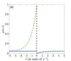
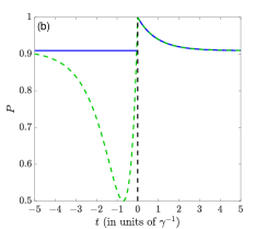
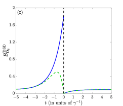
Figure 2: (a) The filtered and smoothed probability of the system being in the excited state. Before the jump (at time $t=0$) the smoothed state begins to increase until it reaches unity right before the jump. (b) The purity for the filtered (blue line) and smoothed (green dashed line) states. The purity of the smoothed state begins to decrease before the jump due to the state having access to the future measurement record. (c) The past-future expected cost function for the filtered, using Eq. (27), and smoothed, using Eq. (14), states. The expected cost for the smoothed estimate of the state is seen to be a better estimator than the filtered estimate due to its smaller expected cost before the jump. In all cases, we have taken $\epsilon=0.05\gamma$ and the limit $\delta\to 0^{+}$.

To gain some physical understanding of $\rho_{\text{S}}^{\rm cl}(t)$ in this system, let us compare it to the filtered state. We can see in Fig. 2 (a), that, unsurprisingly, prior to the jump occurring at $t=0$, the filtered state (solid blue line) remains in its steady state $\wp_{\text{F}}^{\rm ss}(e)=\epsilon/(\gamma+\epsilon)$ until the jump where upon it is projected into the ground state. The smoothed quantum state (dashed green line), on the other hand, begins to diverge from the filtered state as the jump approaches and just prior to the jump reaches the excited state before it is projected to the ground state. This divergence is expected as the smoothed state ‘knows’ that a jump is about to occur, as it is conditioned on the future measurement record. Furthermore, since the true state can only be in either the ground or excited state, it means that for a jump to occur the system must have been in the excited state.

If we look at the purity of the filtered and smoothed quantum state in Fig. 2 (b), we see that as the smoothed quantum state begins to deviate from the filtered state, the purity begins to drop rapidly. Such a drop is not surprising as in order for the smoothed state to reach the excited state it must pass through the maximally mixed state, resulting in the smoothed quantum state having minimal purity prior to the jump. However, this brings up an interesting point. From Eq. (14), we know that the expected cost function for the optimal state is equal to the average difference between the purity of the true state and the conditioned state. However, for this system, the true state is pure irrespective of the unobserved measurement record and Eq. (14) reduces to the impurity of the conditioned state. This means that, since the purity of the smoothed state decreases below that of the filtered state just prior to the jump, the filtered state seemingly gives a lower expected cost function and would be the optimal estimator of the true state, not the smoothed quantum state. However, this is not true, as stated earlier and proved in Ref. Laverick et al. (2021c).

The issue lies in how the expected cost function is calculated for the filtered state. Using Eq. (14) for the filtered state assumes that one only has access to Alice’s past measurement record, whereas the smoothed quantum state assumes that the past-future record is available. Thus, to compare the expected cost function of the filtered state to that of the smoothed state one must take the future measurement record into account and compute

$${\cal B}_{{\bf O}_{\text{S}}}^{\rm TrSD}[\rho_{\text{F}}]=1-2\text{Tr}[\rho_{\text{F}}\rho_{\text{S}}]+P(\rho_{\text{F}})\,.$$ (27)

Note, this argument also holds for classical systems, with the appropriate analogues of the states and cost function. When computing the expected cost function of the filtered state in this way, we see, in Fig. 2 (c), that the smoothed quantum state has the lower expected cost function.

V Proof of Result 1: Bob uses X-Homodyne measurements

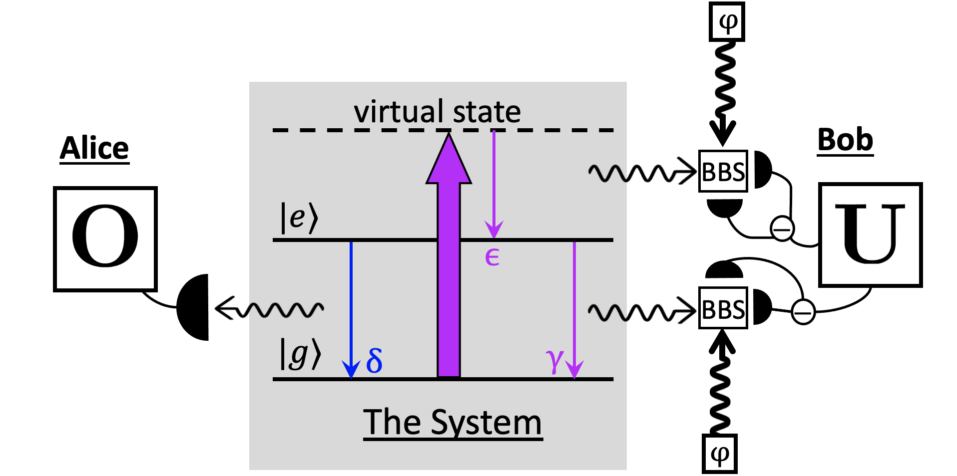
Figure 3: The same physical system as in Fig. 1 with Bob now measuring his $\gamma$ and $\epsilon$ channels both (independently) using X-homodyne measurements (with local oscillator phase $\varphi=0$). Here BBS stands for balanced beam splitter.

In this section we prove, by considering a different measurement choice for Bob, that the smoothed quantum state need not equal the classically smoothed quantum state. Here, instead of photon detection, Bob (perfectly) monitors the unobserved channels each with homodyne measurements. That is, the output light of the system is combined together with a local oscillator with phase $\phi$ on a 50:50 beam splitter, at which point, both outputs of the beam splitter are measured with photon detectors. The single two signals are then subtracted yielding quadrature information about the system. See Fig. 3. Specifically, the measurement current obtained is Wiseman and Milburn (2010); Guevara and Wiseman (2020)

$$J_{k}{\rm d}t=\langle{\hat{c}_{{\rm u},k}e^{i\phi_{k}}-\hat{c}_{{\rm u},k}^{\dagger}e^{-i\phi_{k}}}\rangle{\rm d}t+{\rm d}W_{k}\,,$$ (28)

where $k=\gamma,\epsilon$, $\phi_{k}$ is the local oscillator phase for the $k$-channel, and ${\rm d}W_{k}$ is the innovation, an infinitesimal Wiener increment satisfying

$$\mathbb{E}\{{\rm d}W_{k}\}=0\,,\qquad{\rm d}W_{k}{\rm d}W_{k}^{\prime}=\delta_{kk^{\prime}}{\rm d}t\,.$$ (29)

Such a monitoring causes the true state to evolve according to the stochastic master equation Wiseman and Milburn (2010)

$$\begin{split}{\rm d}\rho_{\text{T}}=&\,{\cal G}[\hat{c}_{\text{o}}]\rho_{\text{T}}{\rm d}N_{\text{o}}-\frac{1}{2}{\cal H}[\hat{c}_{\text{o}}^{\dagger}\hat{c}_{\text{o}}]\rho_{\text{T}}{\rm d}t\\ &\qquad\qquad+{\cal D}[\hat{\bf c}_{\text{u}}]\rho_{\text{T}}{\rm d}t+{\cal H}[\color[rgb]{0,0,0}\hat{\bf c}_{\phi}{\rm d}{\bf W}\color[rgb]{0,0,0}]\rho_{\text{T}}\,.\end{split}$$ (30)

Here $\hat{\bf c}_{\phi}=[\hat{c}_{{\rm u},\gamma}e^{i\phi_{\gamma}},\hat{c}_{{\rm u},\epsilon}e^{i\phi_{\epsilon}}]$ and ${\rm d}{\bf W}=[{\rm d}W_{\gamma},{\rm d}W_{\epsilon}]^{\top}$. From this point forward, we will consider the case where $\phi_{\gamma}=\phi_{\epsilon}=0$, i.e., X-homodyne measurements on both channels. Note, this is called an X-homodyne measurement since the measurement current only contains information about the $x$-component of the Bloch vector ${\bf r}=(x,y,z)^{\top}$ that characterizes the state of the qubit, where $\rho=\mbox{$\frac{1}{2}$}(\hat{1}+{\bf r}\cdot\hat{\bm{\sigma}})$ and $\hat{\bm{\sigma}}=(\hat{\sigma}_{x},\hat{\sigma}_{y},\hat{\sigma}_{z})^{\top}$. The analysis that is to follow would also hold, in this system, for any choice of homodyne phase $\phi_{\gamma}=\phi_{\epsilon}=\phi$.

The important part about this measurement scheme for Bob is that, between two observed jumps, $\rho_{\text{T}}$ is not restricted to the set $\{|{g}\rangle\langle{g}|,|{e}\rangle\langle{e}|\}$, but instead can be in any pure state on the $x$-$z$ great circle of the Bloch sphere. The true state is pure between jumps because it starts in the (pure) ground state and remains pure since the system is perfectly monitored by both Alice and Bob. As for why the pure state can be confined to the $x$-$z$ great circle of the Bloch sphere, this is because, without Bob’s measurement, the quantum state is confined to the $z$-axis of the Bloch sphere and conditioning on an X-homodyne measurement will only give information about the $x$-component of the Bloch vector. Hence, the true state will, typically, have a non-zero $x$-component, whilst the $y$-component will remain zero.

To prove this more rigorously, one can obtain the stochastic differential equations for the Bloch vector of the true state from Eq. (30) subject to the initial condition $\rho_{\text{T}}(t_{1}^{+})=|{g}\rangle\langle{g}|$ and a no-jump record ${\rm d}N_{\text{o}}(t)=0$. We will again take the limit $\delta\to 0^{+}$ to simplify the computation. For this measurement scenario we have

$${\rm d}z =\left[-\gamma(1+z)+\epsilon(1-z)\right]{\rm d}t$$

$$\qquad\qquad-\sqrt{\gamma}x(1+z){\rm d}W_{\gamma}+\sqrt{\epsilon}x(1-z){\rm d}W_{\epsilon}\,,$$ (31)

$${\rm d}y =y\left[-\frac{1}{2}(\gamma+\epsilon){\rm d}t-\sqrt{\gamma}x{\rm d}W_{\gamma}-\sqrt{\epsilon}x{\rm d}W_{\epsilon}\right]\,,$$ (32)

$${\rm d}x =-\frac{1}{2}(\gamma+\epsilon)x{\rm d}t+\sqrt{\gamma}(1+z-x^{2}){\rm d}W_{\gamma}$$ (33)

$$\qquad\qquad\qquad\qquad\qquad+\sqrt{\epsilon}(1-z-x^{2}){\rm d}W_{\epsilon}\,,$$ (34)

with $z(t_{1}^{+})=-1$ and $y(t_{1}^{+})=x(t_{1}^{+})=0$. With these equations we see that, due to the initial condition, the $y$-component will remain zero until the next observed jump.

Since the true state is restricted to the $x$-$z$ great circle, we can reparametrize the true state by the angle $\theta$ of $y$-rotation from the positive $z$-axis instead of the Bloch vector. That is, defining

$$\rho_{\text{T}}(\theta;t)=\mbox{$\frac{1}{2}$}(\hat{1}+\sin\theta(t)\hat{\sigma}_{x}+\cos\theta(t)\hat{\sigma}_{z})\,,$$ (35)

we have ${\mathbb{T}}_{t}=\{\rho_{\text{T}}(\theta;t):\theta\in[0,2\pi)\}$ for all $t\in(t_{1},t_{2})$. With this $\theta$-parametrization we can reduce the evolution of the true state between two observed jumps to a single stochastic differential equation for $\theta$. Using the Itô formula Gardiner (2004); Wiseman and Milburn (2010) to move from a differential equation in $\cos\theta$ (or $\sin\theta$) to one in $\theta$, we obtain

$${\rm d}\theta=A(\theta){\rm d}t+B_{\gamma}(\theta){\rm d}W_{\gamma}+B_{\epsilon}(\theta){\rm d}W_{\epsilon}\,.$$ (36)

Here, $A(\theta)=\sin\theta[\mbox{$\frac{1}{2}$}(\gamma+\epsilon)\cos\theta+(\gamma-\epsilon)]$, $B_{\gamma}(\theta)=\sqrt{\gamma}(1+\cos\theta)$ and $B_{\epsilon}(\theta)=-\sqrt{\epsilon}(1-\cos\theta)$.

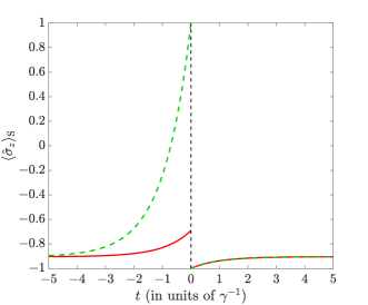
Figure 4: Comparing the conditional average of the $z$-component of the Bloch vector when Alice’s measurement record is obtained by photon detection and Bob’s measurement record is obtained by either photon detection (green dashed line) and an X-homodyne (red line) measurement. Here, we have taken $\delta\to 0^{+}$ and $\epsilon=0.05\gamma$ and an observed detection (jump) occurs at time $t=0$. The $z$-component for the smoothed state using an X-homodyne measurement for Bob differs from the classically smoothed state despite the filtered state being diagonal in the $\hat{\sigma}_{z}$-basis, proving result 1.

We can now begin to compute the smoothed quantum state for this case. From Eq. (15), we have

$$\begin{split}\rho_{\text{S}}(t)&=\int_{0}^{2\pi}\wp(\theta;t|\overleftrightarrow{\bf O})\rho_{\text{T}}(\theta){\rm d}\theta\\ &\propto\int_{0}^{2\pi}\text{Tr}[\hat{E}_{\text{R}}(t)\rho_{\text{T}}(\theta)]\wp(\theta;t|\overleftarrow{\bf O}_{t})\rho_{\text{T}}(\theta){\rm d}\theta\,.\end{split}$$ (37)

As we are only considering the evolution between two observed jumps, we only need to find $\wp(\theta;t|\overleftarrow{\bf O}_{t})=\wp(\theta;t|{\rm N.J.})$, as the retrofiltered effect can be computed via Eq. (22). Here the conditioning ${\rm N.J.}$ stands for a no-jump record. Since Eq. (36) is in the form of a Langevin equation, it can be mapped to a Fokker-Planck equation Gardiner (2004); Gambetta and Wiseman (2005); Wiseman and Milburn (2010); Chantasri et al. (2021) describing the evolution of the probability density of $\theta$ for unknown Wiener processes. However, since Eq. (36) assumes a no-jump observed record, the probability density the Fokker-Planck equation describes is in fact $\wp(\theta;t|{\rm N.J.})$. For this Langevin equation, the corresponding Fokker-Planck equation is

$$\begin{split}\partial_{t}\wp(\theta;t|{\rm N.J.})=&-\partial_{\theta}A(\theta)\wp(\theta;t|{\rm N.J.})\\ &\,\,\,\,+\frac{1}{2}\sum_{k\in\{\gamma,\epsilon\}}\partial_{\theta}^{2}B_{k}(\theta)^{2}\wp(\theta;t|{\rm N.J.})\,,\end{split}$$ (38)

where $\partial_{x}=\partial/\partial x$, with the initial condition $\wp(\theta;t_{1}^{+}|{\rm N.J.})=\delta(\theta-\pi)$ corresponding to the ground state and the boundary condition $\wp(0;t|{\rm N.J.})=\wp(2\pi;t|{\rm N.J.})$. We solve this Fokker-Planck equation numerically using Mathematica’s NDSolve function with a Gaussian initial condition $g(\theta;\mu=\pi,V=0.01\gamma)\approx\delta(\theta-\pi)$, where the mean of the Gaussian is $\mu$ and variance $V$. With the probability density found, we can now compute the smoothed quantum state in the X-homodyne case for comparison to the photon detection case.

As an aside, in general, to calculate the smoothed quantum state requires using an ensemble of unnormalized true states generated according to an ostensible probability distribution. See, for example, Refs. Guevara and Wiseman (2020); Chantasri et al. (2021). That is, one must calculate an extra stochastic variable, the norm of each possible true state. This applies, in general, even in the current simple system where we can generate the ensemble of true states by solving a Fokker-Planck equation. Specifically, the Fokker-Planck equation must be modified to describe the joint probability of $\theta$ and the normalization Gambetta and Wiseman (2005); Chantasri et al. (2021). In the present case, however, since we are considering the limit $\delta\to 0^{+}$, the amount of information Alice gains from a no-detection event is negligible, as this is almost always the result, causing the equation of the true state to reduce to just the unobserved evolution. Since the actual probabilities, for this case, can be computed easily from the distributions for ${\rm d}W_{\gamma}$ and ${\rm d}W_{\epsilon}$, the normalized equation for the true state can be used.

We can now begin to compute the smoothed quantum state. We can see that, in this homodyne case, the smoothed quantum state will be diagonal in the $\hat{\sigma}_{z}$-basis because of a symmetry in the dynamics. Specifically, since there are no unitary dynamics driving the system in a particular way, for any unobserved measurement record that causes the true state to rotate clockwise on the $x$-$z$ great circle, there is an equally likely record of the opposite sign that causes the state to evolve in exactly the same way in the counter-clockwise direction. Importantly, it is equally likely even given the future record (the jump) that Alice observes because the excited state probability is the same for both directions of rotation. Thus, when Alice averages over the possible unobserved records, each true state can be paired with its mirror image about the $z$-axis, cancelling the $x$-component of the Bloch vector.

We can thus easily compare the X-homodyne smoothed quantum state with the classically smoothed quantum state by only looking at their $z$-components. As Fig. 4 shows, there is a clear difference between them. (As explained in Sec. IV.2, in the limit $\delta\to 0^{+}$ we need be concerned only with the smoothed quantum state in a time of order $1/(\gamma+\epsilon)$ before the final jump.) Thus, by this example, we have proven our first result: the commuting of the filtered state and retrofiltered effect is not sufficient for $\rho_{\text{S}}(t)$ to equal $\rho_{\text{S}}^{\rm cl}(t)$.

In this example, the obvious difference between the smoothed state obtained classically (when Alice assumes an orthogonal basis for the true state) and that obtained when Bob performs a homodyne measurement (when Alice takes this into account) is the value of $z$ for the smoothed state immediately prior to the jump. We can intuitively understand this as follows. Since the true state in the latter case can be in a superposition of both the ground and excited state, as opposed to just being in one of these states, a jump can occur even when the system is not in the excited state. Thus, when Alice is estimating the true state using smoothing, she cannot be certain that the true state was in the excited state just prior to the transition, unlike in the classical (photon detection) case where she is certain. As such, her smoothed estimate in the homodyne case only moves somewhat closer to the excited state as the jump approaches.

VI Proof of Result 2: Bob uses an adaptive measurement

In the preceding section, the non-classical smoothed state was still diagonal in the same basis as the classical smoothed state, and therefore diagonal in the same basis as the filtered state and retrofiltered effect (whose co-diagonality defines the scenario we are investigating). In this section we show the stronger result that the smoothed quantum state is not necessarily even co-diagonal with $\rho_{\text{F}}$ and $\hat{E}_{\text{R}}$. As we saw in the X-homodyne example, the smoothed quantum state was diagonal in the $\hat{\sigma}_{z}$-basis because Bob’s measurement gave the set of possible true states a symmetry about the $z$-axis of the Bloch sphere. To avoid reasoning of this sort for this final case, Bob’s measurement is chosen to break this symmetry in the set of possible true states.

To achieve an asymmetric distribution of true states, we allow Bob to use an adaptive measurement involving finite strength local oscillators on the unobserved channels; see Fig. 5. Here, “finite strength” means that the local oscillator intensity is comparable to the intensity of light emitted by the system, so the detection still resolves individual photons (unlike the strong local oscillator case of a homodyne measurement). The measurement is “adaptive” in the sense that after every detection event, the amplitude (strength and phase) of the local oscillators can be changed, depending on the current settings of these amplitudes, and the type of photodection that occurs (if more than one detector is used, which is the case for our system here, with two unobserved channels). Measurements of this kind have been studied theoretically for many decades Dolinar (1973); Helstrom (1976); Wiseman and Toombes (1999); Karasik and Wiseman (2011); Wiseman and Gambetta (2012); Daryanoosh and Wiseman (2014); Warszawski and Wiseman (2019a, b).

A non-trivial property of adaptive measurements of the sort described is that they can constrain the stochastic evolution of the true state of the system to a finite and time-independent set ${\mathbb{T}}$. Note the lack of a subscript $t$. Together with the corresponding stationary probabilities of each state in ${\mathbb{T}}$, this comprises a so-called physically realizable ensemble (PRE) Wiseman and Vaccaro (2001); Karasik and Wiseman (2011). The significance of “physically realizable” here is as follows. Consider a Markovian (in the strongest sense Li et al. (2018)) open quantum system whose unconditional evolution is described by a Lindblad master equation, where, in the long-time limit, $t\geq t^{\rm ss}$, the system reaches a unique stationary solution that is mixed. Owing to the fact that a mixed quantum state can be decomposed into a weighted ensemble of pure states in infinitely many ways, there are different interpretations of how the underlying pure state dynamics of the system unfold. However, only some of these pure state ensembles are physically realizable, meaning that there exists a way to continuously monitor the environment (without affecting the unconditional evolution) such that the conditioned state at times after $t^{\rm ss}$ is confined to ${\mathbb{T}}$ with the corresponding probabilities being realized in the ergodic sense.

The classical ensemble of Sec. IV.2, with ${\mathbb{T}}=\{|{g}\rangle\langle{g}|,|{e}\rangle\langle{e}|\}$, is an example of such a PRE, but in general the states in ${\mathbb{T}}$ need not be orthogonal Wiseman and Toombes (1999); Karasik and Wiseman (2011); Daryanoosh and Wiseman (2014); Warszawski and Wiseman (2019a, b). This is essential for finding an asymmetric (under application of $\hat{\sigma}_{z}$) steady-state ensemble. (In our case, this steady state means a long time, compared to $1/(\gamma+\epsilon)$, after Alice’s last jump, which is always the limit we can consider when Alice’s jump rate $\delta\to 0^{+}$; see more below.) For our system, the particular adaptive measurement scheme is chosen so that ${\mathbb{T}}$ comprises three states, with no symmetry under application of $\hat{\sigma}_{z}$. The conditioned dynamics causes the true state to cyclically transition between these states. This is possible only in certain parameter regimes, which is why we chose $\epsilon=0.05\gamma$.

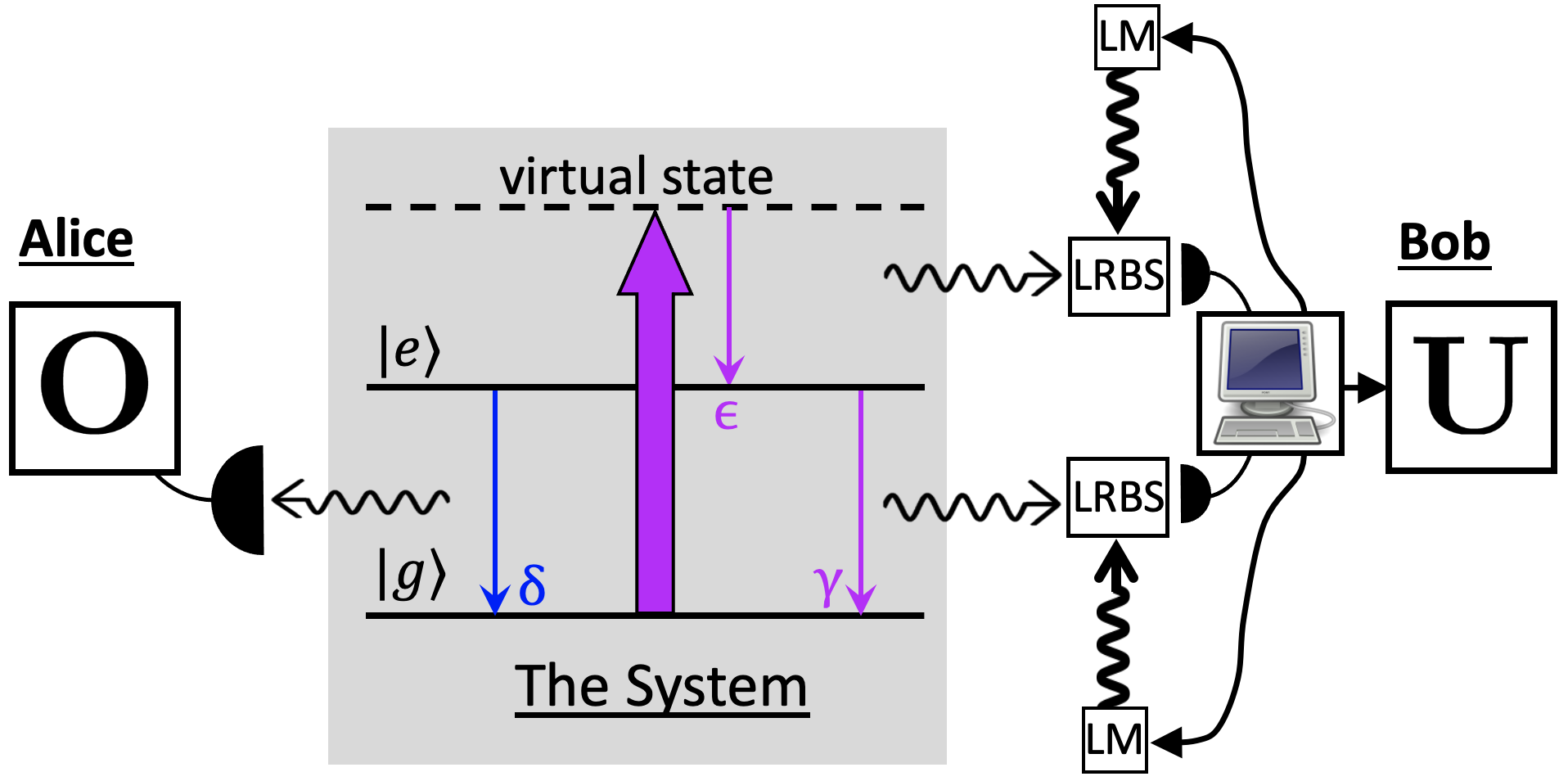
Figure 5: The same physical system in Fig. 1 with Bob using the adaptive measurement scheme in App. B. In this figure, LRBS stands for low-reflectivity beam splitter and LM stands for light modulator.

A detailed discussion of PREs in the context of the photon emission and absorption master equation is given in Refs. Warszawski and Wiseman (2019a) §4.4.2. In our case, the scenario is modified slightly as it is Bob’s measurement record which causes Alice’s filtered state (as opposed to the unconditioned state) to become pure upon conditioning. That is, we make the substitution $\rho\to\rho_{\text{F}}$ and it is Bob’s measurement that causes the true state to become pure when deriving the PRE for the system. Note, there is a subtlety in regards to the filtered state that one should be aware of when making this substitution. In the standard PRE scenario, it is necessary for the unconditioned state to have reached a unique stationary solution. However, the filtered state is a stochastic quantity and in general will not reach a unique stationary solution in the long-time limit. As such, there are only select cases, i.e., when the filtered state (or some deterministic property of the state Laverick et al. (2021a)) reaches a unique steady state, that we can apply the PRE theory in this manner.

In the example that we consider, such a steady-state will usually exist for the filtered state, provided the time between consecutive jumps, $\tau$, is typically much longer than the time in which the system equilibriates. More formally, when $\tau=(\delta\langle{e}|\rho|{e}\rangle)^{-1}\gg(\gamma+\epsilon+\delta)^{-1}$. Since, after the first jump, $\rho(t_{1})=|{g}\rangle\langle{g}|$, it will always be the case that $\langle{e}|\rho|{e}\rangle\leq\langle{e}|\rho^{\rm ss}|{e}\rangle=\epsilon(\gamma+\epsilon+\delta)^{-1}$. Thus, the filtered state is likely to reach steady state between consecutive jumps if we operate in the parameter regime

$$\delta\epsilon\ll(\gamma+\epsilon+\delta)^{2}\approx(\gamma+\epsilon)^{2}\,,$$ (39)

where, for the final approximation, we have assumed $\delta\ll\gamma+\epsilon$. Note, for the parameter regime we have been considering thus far ($\epsilon=0.05\gamma$), we require that $\delta\ll 22\gamma$. As has been the case for the other measurement scenarios, we will, for simplicity, take the limit $\delta\to 0^{+}$.

For the stationary solution of the filtered state in this example,

$$\rho_{\text{F}}^{\rm ss}=\frac{\epsilon}{\gamma+\epsilon}|{e}\rangle\langle{e}|+\frac{\gamma}{\gamma+\epsilon}|{g}\rangle\langle{g}|\,,$$ (40)

the cyclic physically realizable ensemble $\{\rho(\theta),\wp_{\theta}\}_{\theta\in\{\alpha,\beta,\phi\}}$ chosen, from the possible valid ensembles, is displayed in Fig. 6 with the angles and corresponding probability weights. It should be emphasized that the implemented measurement strategy Warszawski and Wiseman (2019a) only causes the true state to undergo the cyclical dynamics depicted in Fig. 6 when the filtered state is in steady state. Outside of this regime the dynamics of the true state may be more complicated, but when averaged still result in the transient dynamics of the filtered state. The reader is referred to App. B for the local oscillator settings that achieve the PRE shown in Fig. 6.

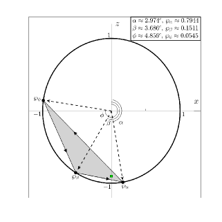
Figure 6: The $x$-$z$ great circle of the qubit’s Bloch sphere showing  the cyclic physically realizable ensemble chosen for the example qubit system subject to the measurement scheme in Fig. 5 plotted on the $x$-$z$ great circle. The three black points on the circle are the three pure states in the ensemble with there corresponding angles and occupation probabilities given in the top right corner (see Ref. Warszawski and Wiseman (2019a) for how these are calculated) and the arrows connecting them shows the cyclic dynamics that results from the adaptive measurement strategy. The shaded region is where both the filtered and smoothed quantum state must reside at times after $t^{\rm ss}$. Lastly, the square marker indicates $\rho_{\text{F}}^{\rm ss}$. See Fig. 4 for the parameter details.

With the measurement scheme and dynamics of the true quantum state covered we can now begin to compute the smoothed quantum state for this case. As in the previous two cases, the smoothed quantum state differs from the filtered state only for a time of order $1/(\gamma+\epsilon)$ prior to the second observed jump. As such we only need to compute the smoothed quantum state when the retrofiltered effect is outside of steady state. Since we are working in the limit as $\delta\to 0^{+}$, it will typically (in the strict sense) be the case that enough time has passed for the filtered state to have reached steady state well before the next jump. As such, over the time prior to the second jump that we are interested in, the true state will be cyclically jumping between the three pure states in the PRE. Thus the smoothed quantum state over this time region can be computed via

$$\rho_{\text{S}}(t)\propto\sum_{\theta\in\{\alpha,\beta,\gamma\}}\text{Tr}\left[\hat{E}_{\text{R}}(t)\rho(\theta)\right]\wp(\theta;t|\overleftarrow{\bf O}_{t})\rho(\theta)\,.$$ (41)

All that remains to compute the smoothed quantum state is to determine the probability distribution $\wp(x|\overleftarrow{\bf O}_{t})$. This distribution is, by definition, the occupation probabilities of the PRE states, i.e., $\wp(\theta;t|\overleftarrow{\bf O})=\wp_{\theta}$.

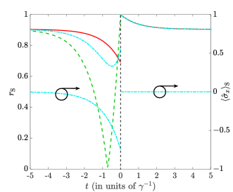
Figure 7: The length (left-hand-side axis) and the $x$-component (right-hand-side axis) of the Bloch vector for the smoothed quantum state when Alice’s measurement record is obtained by photon detection and Bob’s record by either photodetection (green dashed line), X-homodyne (red solid line), or an adaptive weak local oscillator (cyan dot-dashed line). The $x$-component of the smoothed state when Bob implements photodetection or an X-homodyne measurement are not shown as they are zero at all times.

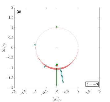
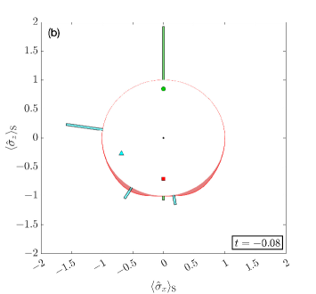
Figure 8: (a) and (b) show the $x$-$z$ great circles of the Bloch sphere plotted at two different times prior to the observed jump. On the surface of the circle we have plotted the probability distributions for the case where Bob measures the environment using photodetection (green), an X-homodyne (red), and an adaptive scheme (cyan) (all of which have a zero $y$-component). The relative area of the bars indicates the occupation probability for that state. Note, the total area of both the the green and cyan bars are equal but the area under the red curve has been scaled by a factor of $3$ for clarity. The markers (circle, square and triangle) on the interior correspond to the smoothed mean using the correspondingly coloured distribution. See Fig. 4 for the parameter details.

To check whether the smoothed quantum state is non-diagonal in the $\hat{\sigma}_{z}$-basis, we only need to look at the $x$-component of its Bloch vector, as the $y$-component is always zero for this adaptive local oscillator scheme. In Fig. 7, the $x$-component (right-hand-axis) and the length of the Bloch vector (left-hand-axis), defined as $r=\sqrt{\langle{\hat{\sigma}_{x}}\rangle^{2}+\langle{\hat{\sigma}_{y}}\rangle^{2}+\langle{\hat{\sigma}_{z}}\rangle^{2}}$, for the smoothed quantum state are shown for this scheme (cyan). There are a couple of interesting features in this example, the most important being that the Bloch vector of the smoothed quantum state prior to the jump has non-zero $x$-component. Thus, the smoothed quantum state is not diagonal in the $\hat{\sigma}_{z}$-basis, the shared basis of the filtered state and retrofiltered effect, proving our second result.

The reason the smoothed quantum state becomes non-diagonal is that Alice is able to infer from $\overrightarrow{\bf O}_{t}$, specifically the upcoming jump, that the two states in the PRE with a negative $x$-component are more likely to have been occupied than they otherwise would be. This is because they have a larger overlap with the excited state than the single state with a positive $x$-component. This breaks the symmetry of reflection around the $z$-axis. This is evident in Fig. 8, where we can see the clear increase in the probability of the true state being in the PRE state on the far left and a substantial decrease in the probability of being the PRE state closest to the ground state.

It should also be apparent, since the smoothed quantum state will be a mixture of the states in the PRE over the interval of interest, that the Bloch vector will lie within the triangle formed by the PRE states (the grey shaded area in Fig. 6). As a result, the smoothed quantum state will not pass through the maximally mixed state (the centre of the circle) as the observed jump approaches. This is not to say that the length of the Bloch vector does not decrease, just that it does not go to zero. This can bee seen in Fig. 7.

VII Proof of Result 3: Comparing the expected cost functions

As we have just seen in the last two examples, the commutativity of the filtered state and retrofiltered effect imposes no apparent constraints on the dynamics of the optimal smoothed quantum state. However, the fact that the optimal estimates in these cases are different gives rise to a new question. Alice cannot compute her optimal smoothed quantum state without knowledge of the nature of Bob’s measurement, as this determines the set of possible true states. But what is the ‘best’ measurement unravelling for Bob to perform, from Alice’s point of view? Since we already have a metric, the expected cost function, whose minimization defines the optimal estimate ($\rho_{\text{F}}$ or $\rho_{\text{S}}$), it seems natural to use that expectation value as a measure of how good Alice’s estimate is. For our particular cost function, this is equivalent to the measurement that results in the purest smoothed state.

Now, intuitively, the measurement for Bob that would give the greatest purity would be the measurement that causes $\rho_{\text{S}}(t)=\rho_{\text{S}}^{\rm cl}(t)$ as Alice only has to estimate between perfectly distinguishable true states. Applying this type of logic to the three cases that we have already considered, one would guess that after the case where Bob uses photon detection (having two perfectly distinguishable true states), the next best case would be the adaptive scheme (with three non-orthogonal true states), followed by the X-homodyne case (with a continuous infinity of non-orthogonal state to distinguish). Comparing the expected cost functions for each estimate in Fig. 9, we can see that the above intuition is incorrect. In fact, the complete opposite holds over the majority of the time. This is despite the fact that the classically smoothed quantum state $\rho_{\text{S}}^{\rm cl}(t)$ is pure immediately prior to the jump occurring. Actually we have already discussed how this is linked with a prior decrease in purity in the classical case, in Sec. IV.2. With only two states, with the steady state being relatively close to the ground state, and with the state just prior to the jump being the excited state, the classical smoothed state must pass through the maximally mixed state, at which point it must be the worst (highest expected cost) estimator. This leads us to our final result, that the classically smoothed quantum state does not necessarily yield the lowest expected cost function.

We can gain a more general intuition as to why increasing the number of possible true states yields purer smoothed estimates, by analyzing the expression for the purity. That is,

$$\begin{split}P_{\text{S}}(t)&=\text{Tr}[\rho_{\text{S}}(t)^{2}]\\ &=\text{Tr}\left[\left(\sum_{\rho_{\text{T}}\in{\mathbb{T}}_{t}}\wp(\rho_{\text{T}};t|\overleftrightarrow{\bf O})\rho_{\text{T}}\right)^{2}\right]\\ &=\sum_{\rho_{\text{T}},\rho_{\text{T}}^{\prime}\in{\mathbb{T}}_{t}}\wp(\rho_{\text{T}};t|\overleftrightarrow{\bf O})\wp(\rho_{\text{T}}^{\prime};t|\overleftrightarrow{\bf O})\text{Tr}[\rho_{\text{T}}\rho_{\text{T}}^{\prime}]\,,\end{split}$$ (42)

where for ease of illustration we have assumed a discrete set of possible true states. We see that the purity is a weighted sum of the overlap between possible true states. Thus, with only two orthogonal true states in ${\mathbb{T}_{t}}$, the only terms that contribute are when $\rho_{\text{T}}=\rho_{\text{T}}^{\prime}$. However, as the number of possible true states increase, additional terms that result from non-orthogonal states will also contribute, increasing the sum. Following this intuition, we arrive at the ordering that is observed in Fig. 9, over the great bulk of times. The exception is when the jump is imminent, where the ordering flips. (From Fig. 9, this flipping might appear to happen at an instant, but zooming in one finds that the three line do not intersect at the same point in time.) For the photon detection case the reason for the reversal is clear; as discussed above, just before Alice’s jump the state is pure and so the expected cost is zero. Something similar, but less dramatic, happens with the adaptive jump case. Just before Alice’s jump, one of the three possible true states becomes much more likely than the others, as discussed in Sec. VI. We refer the reader to Fig. 8 again to appreciate the difference from the homodyne case.

As an aside, in Ref. Laverick et al. (2021c) it was shown that the trace-square deviation from the true state is not the only cost function that has the smoothed state as its optimal estimator, so does the relative entropy. One might then ask, does the classically smoothed state give the lowest expected relative entropy? The simple answer is no, in fact the ordering will not change. This is because, as shown in Ref. Laverick et al. (2021c), when the true state is pure, the expected relative entropy between the smoothed state and the true state reduces to the von-Neumann entropy. Since, for qubits, the von-Neumann entropy is a monotonic function of the purity, the ordering will remain.

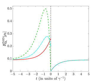
Figure 9: The expected cost of the smoothed state when Alice’s measurement record is obtained by photon detection and Bob’s record is obtained by either photon detection (green dashed line), X-homodyne (red line) or by an adaptive strategy based on weak local oscillators (cyan dot-dashed line) (see Sec. VI. The expected cost for both the X-homodyne case and the adaptive weak local oscillator cases have a lower expected cost than the photon detection (classical) case for most times due to the latter having to pass through the maximally mixed state to reach the (pure) excited state. See Fig. 4 for the parameter details.

VIII Conclusion

In this paper we have proved three results regarding quantum state smoothing. These three results were motivated by the application of classical smoothing techniques in quantum experiments. These experiments assumed the unobserved information in the environment was made classical in a way that removed the ‘quantumness’ from the system. Specifically, the quantum system was effectively replaced by a classical system, always in one of a set of orthogonal states with dynamics described by an hidden Markov model.

One might say that these assumptions were physically reasonable in the context of these experiments. However, we argue that it is important to state an assumption like this explicitly, because in its absence one cannot justify the application of classical smoothing techniques for a quantum state. Our argument is established by our first result, and is backed up by two even stronger negative results, regarding the applicability or usefulness of classical smoothing techniques. All three of the results in our paper were proven using a simple qubit system (atom) coupled to three decoherence channels. The measurements by the observer (Alice) has a classical description, describable in terms of transitions between the ground and excited states, and the master equation has no terms that generate coherence between these states.

Our first result was to show that the optimal smoothed estimate for this system in this situation depends on how the information unobserved by Alice in the environment is assumed to become classical. In particular, we here considered two potential measurement unravellings for the environment, which for convenience we call Bob’s measurement schemes. For photon detection, which is equivalent to assuming an orthogonal hidden Markov model for this system, the classical smoothed state (probability distribution over the two orthogonal states) is recovered. But for homodyne detection a different smoothed state is found, albeit still a mixture of the states in the classical model.

Our second result was that one cannot even make a statement on the diagonal basis of the smoothed quantum state without knowing the unravelling of the unobserved information. For this we considered a third type of measurement for Bob: an adaptive strategy using local oscillators and photon counters. Under this scheme, despite the apparent classicality of Alice’s measurement, the smoothed quantum state is not, in general, a mixture of ground and excited states.

Our third and final result is the most subtle. In the face of the first two results, one might still hope that the classical smoothing technique would be better than the other techniques; that the simplicity of the photon detection scheme for Bob, relative the others (homodyne and adaptive), would be reflected in Alice’s ability to estimate the resulting unknown record and hence estimate the associated true state. (This ability is quantified by the trace squared deviation between the true state and the state estimate, which is the cost function whose minimization defines the optimal estimate.) Contrary to this intuition, we showed in our example that, most of the time, the expected cost is higher for the classical smoothing technique than for the quantum smoothing technique appropriate for the other unravellings.

Our results raise several questions for future research. Whilst we have shown that a classical description of Alice’s filtering and retrofiltering is not sufficient for classical smoothing to be applicable in general, and that a classical description of the true state is sufficient, we do not know whether the latter condition is necessary, or whether some weaker condition would be sufficient. Another question is whether, given a classical description of Alice’s filtering and retrofiltering, there could be a different cost function such that the classically smoothed quantum state in Eq. (11) would be the optimal estimator for quantum systems. Another way that one might try to apply classical smoothing would be to diagonalize the filtered state at each instant in time and then compute new weightings for those eigenstates using classical smoothing. Lastly, as mentioned in Ref. Chantasri et al. (2019), it would be interesting to investigate what would happen if Alice assumed that Bob’s unravelling had a classical description when in fact it does not. How poorly does this ‘wrong-guessed’ smoothed state perform in terms of the trace-square distance, and could we find unravellings for Bob (or even Alice) that minimizes the deviation from the optimal expected cost?

Appendix A Co-diagonality of the filtered state and retrofiltered effect

In this appendix we prove that when $\rho_{\text{T}}(t)\in{\mathbb{T}}_{\rm diag}=\{|{\psi_{m}}\rangle\langle{\psi_{m}}|:\langle{\psi_{m}}|\psi_{m^{\prime}}\rangle=\delta_{m,m^{\prime}}\}$, both the filtered state (provided the state is initially diagonal in this basis) and retrofiltered effect are necessarily diagonal in any basis that contains these states. However, before we present the proof, we need to express how both the true and filtered quantum states evolve in terms of quantum maps. For the true quantum state, a measurement operator Breuer and Petruccione (2006); Wiseman and Milburn (2010) is assigned for each measurement outcome, which we will denote as $\hat{M}_{\text{o}}({\bf y}_{\text{o}};t)$, where ${\bf y}_{\text{o}}(t)$ denotes the observed measurement outcome, and similarly for the unobserved measurement, be it a detector click or a photocurrent. With these measurement operators, the true state evolves as Guevara and Wiseman (2020)

$$\tilde{\rho}_{\text{T}}(t+{\rm d}t)=\hat{M}_{\text{o}}({\bf y}_{\text{o}};t)\hat{M}_{\text{u}}({\bf y}_{\text{u}};t)\tilde{\rho}_{\text{T}}(t)\hat{M}_{\text{u}}^{\dagger}({\bf y}_{\text{u}};t)\hat{M}_{\text{o}}^{\dagger}({\bf y}_{\text{o}};t)\,.$$ (43)

Here, for a later derivation, we have refrained from normalizing the state at each time step, as indicated by the tilde. Note, for notational simplicity we have absorbed the operator that generates the deterministic part of the evolution (including the Hamiltonian part of the evolution) into the observed measurement operator.

For the filtered quantum state, we condition only on the observed measurement record, with the unobserved channel contributing the decoherence affecting the state. In general, one can recover the appropriate dynamics of the filtered state by averaging over the possible unobserved records. Averaging Eq. (43) over the unobserved measurement record, the (unnormalized) filtered state evolves according to

$$\tilde{\rho}_{\text{F}}(t+{\rm d}t)=\sum_{{\bf y}_{\text{u}}(t)}\hat{M}_{\text{o}}({\bf y}_{\text{o}};t)\hat{M}_{\text{u}}({\bf y}_{\text{u}};t)\tilde{\rho}_{\text{F}}(t)\hat{M}_{\text{u}}^{\dagger}({\bf y}_{\text{u}};t)\hat{M}_{\text{o}}^{\dagger}({\bf y}_{\text{o}};t)\,,$$ (44)

where we have assumed, for simplicity, that the spectrum of measurement outcomes is discrete. For a continuous spectrum this sum is replaced by an appropriate integral. To determine how the retrofiltered effect evolves, we use the fact that $\text{Tr}[\tilde{\rho}_{\text{F}}(t)\hat{E}_{\text{R}}(t)]=\tilde{\wp}(\overleftrightarrow{\bf O})$, which is independent of the time $t$. Thus, we have $\text{Tr}[\tilde{\rho}_{\text{F}}(t)\hat{E}_{\text{R}}(t)]=\text{Tr}[\tilde{\rho}_{\text{F}}(t+{\rm d}t)\hat{E}_{\text{R}}(t+{\rm d}t)]$. Applying Eq. (44), the cyclic property of the trace and the fact that this holds for all possible filtered states gives us the dynamical equation for the retrofiltered effect,

$$\hat{E}_{\text{R}}(t)=\sum_{{\bf y}_{\text{u}}(t)}\hat{M}_{\text{u}}^{\dagger}({\bf y}_{\text{u}};t)\hat{M}_{\text{o}}^{\dagger}({\bf y}_{\text{u}};t)\hat{E}_{\text{R}}(t+{\rm d}t)\hat{M}_{\text{o}}({\bf y}_{\text{o}};t)\hat{M}_{\text{u}}({\bf y}_{\text{u}};t)\,.$$ (45)

Proof: Given that $\rho_{\text{T}}(t)\in{\mathbb{T}}_{\rm diag}$ over the interval $[t_{0},T)$, Eq. (43) becomes

$$|{\psi_{i}}\rangle\langle{\psi_{i}}|\propto\hat{M}_{\text{o}}({\bf y}_{\text{o}};t)\hat{M}_{\text{u}}({\bf y}_{\text{u}};t)|{\psi_{j}}\rangle\langle{\psi_{j}}|\hat{M}_{\text{u}}^{\dagger}({\bf y}_{\text{u}};t)\hat{M}_{\text{o}}^{\dagger}({\bf y}_{\text{o}};t)\,.$$ (46)

By expressing the product of measurement operators as $\hat{M}_{\text{o}}({\bf y}_{\text{o}};t)\hat{M}_{\text{u}}({\bf y}_{\text{u}};t)=\sum_{i,j}T_{i,j}({\bf y}_{\text{u}};t)|{\psi_{i}}\rangle\langle{\psi_{j}}|$, Eq. (46) places a restriction on the matrix elements $T_{i,j}({\bf y}_{\text{u}};t)$. Specifically, we have $T_{i,k}({\bf y}_{\text{u}};t)T^{*}_{k,j}({\bf y}_{\text{u}};t)\propto\delta_{i,j}$, where $A^{*}$ denotes the complex conjugate of $A$. Note, since we are only averaging over the unobserved measurement, we have dropped the dependence on ${\bf y}_{\text{o}}(t)$ in the matrix elements for notational simplicity. Importantly, this constraint holds for all possible realizations of ${\bf y}_{\text{u}}(t)$ since the set ${\mathbb{T}}_{\rm diag}$ contains the possible true states for any realization of $\overleftarrow{\bf O}_{t}$ and $\overleftarrow{\bf U}_{t}$.

With this constraint on the measurement operators, we can now compute the filtered state. Beginning with Eq. (44), we have

$$\tilde{\rho}_{\text{F}}(t+{\rm d}t)=\sum_{{\bf y}_{\text{u}}(t)}\sum_{i,j,k,\ell}T_{ij}({\bf y}_{\text{u}};t)T^{*}_{k\ell}({\bf y}_{\text{u}};t)|{\psi_{i}}\rangle\langle{\psi_{j}}|\tilde{\rho}_{\text{F}}(t)|{\psi_{k}}\rangle\langle{\psi_{\ell}}|\,.$$ (47)

Now, assuming that the filtered state is diagonal at time $t$, i.e., $\tilde{\rho}_{\text{F}}(t)=\sum_{m}\tilde{\wp}_{\text{F}}(m;t)|{\psi_{m}}\rangle\langle{\psi_{m}}|$, then

$$\tilde{\rho}_{\text{F}}(t+{\rm d}t) =\sum_{{\bf y}_{\text{u}}(t)}\sum_{i,j,k,\ell,m}T_{ij}({\bf y}_{\text{u}};t)T^{*}_{k\ell}({\bf y}_{\text{u}};t)\tilde{\wp}_{\text{F}}(m;t)|{\psi_{i}}\rangle\langle\psi_{j}|\psi_{m}\rangle\langle\psi_{m}|\psi_{k}\rangle\langle{\psi_{\ell}}|$$ (48)

$$=\sum_{{\bf y}_{\text{u}}(t)}\sum_{i,j,k,\ell,m}T_{ij}({\bf y}_{\text{u}};t)T^{*}_{k\ell}({\bf y}_{\text{u}};t)\tilde{\wp}_{\text{F}}(m;t)\delta_{j,m}\delta_{m,k}|{\psi_{i}}\rangle\langle{\psi_{\ell}}|$$ (49)

$$=\sum_{{\bf y}_{\text{u}}(t)}\sum_{i,j,\ell}T_{ij}({\bf y}_{\text{u}};t)T^{*}_{j\ell}({\bf y}_{\text{u}};t)\tilde{\wp}_{\text{F}}(j;t)|{\psi_{i}}\rangle\langle{\psi_{\ell}}|$$ (50)

$$=\sum_{{\bf y}_{\text{u}}(t)}\sum_{i,j,\ell}c_{i}({\bf y}_{\text{u}};t)\tilde{\wp}_{\text{F}}(j;t)\delta_{i,\ell}|{\psi_{i}}\rangle\langle{\psi_{\ell}}|$$ (51)

$$=\sum_{{\bf y}_{\text{u}}(t)}\sum_{i,j}c_{i}({\bf y}_{\text{u}};t)\tilde{\wp}_{\text{F}}(j;t)|{\psi_{i}}\rangle\langle{\psi_{i}}|\,,$$ (52)

where, in the Eq. (51), we have substituted in the condition $T_{i,j}({\bf y}_{\text{u}};t)T^{*}_{j,\ell}({\bf y}_{\text{u}};t)=c_{i}({\bf y}_{\text{u}};t)\delta_{i,\ell}$, where $c_{i}({\bf y}_{\text{u}};t)\in{\mathbb{R}}$ is the constant of proportionality. Importantly, we see that the quantum maps that generate the evolution of the filtered state preserve the diagonality in the orthogonal basis $\{|{\psi_{m}}\rangle\}_{m}$. Thus, provided the initial condition is diagonal in the basis $\{|{\psi_{m}}\rangle\}_{m}$, the filtered state will remain diagonal while $\rho_{\text{T}}\in{\mathbb{T}}_{\rm diag}$.

For the retrofiltered effect, the proof follows in a similar manner to that of the filtered state. Beginning by substituting the measurement operator into Eq. (45) and assuming the retrofiltered effect at $t$ is diagonal in this basis, i.e., $\hat{E}_{\text{R}}(t+{\rm d}t)=\sum_{m}E_{\text{R}}(m;t+{\rm d}t)|{\psi_{m}}\rangle\langle{\psi_{m}}|$, we have

$$\hat{E}_{\text{R}}(t) =\sum_{{\bf y}_{\text{u}}(t)}\sum_{i,j,k,\ell,m}T^{*}_{ij}({\bf y}_{\text{u}};t)T_{k\ell}({\bf y}_{\text{u}};t)E_{\text{R}}(m;t+{\rm d}t)|{\psi_{i}}\rangle\langle\psi_{j}|\psi_{m}\rangle\langle\psi_{m}|\psi_{k}\rangle\langle{\psi_{\ell}}|$$ (54)

$$=\sum_{{\bf y}_{\text{u}}(t)}\sum_{i,j,\ell}T^{*}_{ij}({\bf y}_{\text{u}};t)T_{j\ell}({\bf y}_{\text{u}};t)E_{\text{R}}(j;t+{\rm d}t)|{\psi_{i}}\rangle\langle{\psi_{\ell}}|$$ (55)

$$=\sum_{{\bf y}_{\text{u}}(t)}\sum_{i,j,\ell}c_{i}({\bf y}_{\text{u}};t)E_{\text{R}}(j;t+{\rm d}t)\delta_{i,\ell}|{\psi_{i}}\rangle\langle{\psi_{\ell}}|$$ (56)

$$=\sum_{{\bf y}_{\text{u}}(t)}\sum_{i,j}c_{i}({\bf y}_{\text{u}};t)E_{\text{R}}(j;t+{\rm d}t)|{\psi_{i}}\rangle\langle{\psi_{i}}|\,,$$ (57)

where, in Eq. (56), we have used the fact that $T^{*}_{ij}({\bf y}_{\text{u}};t)T_{j\ell}({\bf y}_{\text{u}};t)=(T_{ij}({\bf y}_{\text{u}};t)T^{*}_{j\ell}({\bf y}_{\text{u}};t))^{*}=c_{i}({\bf y}_{\text{u}};t)\delta_{i,\ell}$. Once again, we see that the quantum maps that generate the evolution of the retrofiltered effect preserve the diagonality in the orthogonal basis $\{|{\psi_{i}}\rangle\}_{i}$. Thus, since $\hat{E}_{\text{R}}(T)\propto\hat{1}$, which is diagonal in every basis, the retrofiltered effect is necessarily diagonal when $\rho_{\text{T}}\in{\mathbb{T}}_{\rm diag}$.

$\square$

Appendix B Specification of the adaptive measurement scheme

In this paper the physical system of interest is a qubit coupled to three decoherence channels: two emission channels (one monitored by Alice and one by Bob) and one absorption channel (monitored by Bob). In Sec. VI, the emission channel monitored by Alice is assumed to be very weak, $\delta\rightarrow 0^{+}$, meaning that, in the long time periods between her observed detections, her filtered state will reach a steady state. In some parameter regimes Warszawski and Wiseman (2019a) it is then possible for Bob to restrict the system state to a finite and time-independent set ${\mathbb{T}}$, which is known as a physically realizable ensemble (PRE). In order for this to occur, Bob must use a carefully chosen adaptive measurement scheme to monitor his emission and absorption channels. In Sec. VI, Bob is assumed to enact such a measurement scheme, which leads to the PRE of Fig. 6 when $\epsilon=0.05\gamma$. The PRE in question consists of three states ($\alpha$, $\beta$, $\gamma$) that are labelled by the angle of the Bloch vector in the $x$-$z$ great circle of the Bloch Sphere.

The freedom that Bob has when choosing his measurement scheme is most easily understood in a quantum optics context. Bob may utilise linear interferometers that take the field outputs of the system as inputs. He may also use weak local oscillators (WLOs) that can be added to the interferometer outputs prior to photodetection. To achieve the PRE of Sec. VI, it turns out that Bob can employ a relatively simple measurement scheme that only uses WLOs and does not mix the system outputs. The measurement scheme is further simplified as it obeys symmetries present in the unconditional evolution, namely that real-valued density matrices remain real-valued under the action of the ${\cal L}={\cal D}[\hat{\bf c}]$. Thus Bob separately adds a real-valued WLO to both his emission and absorption channels before photodetection. The scheme is adaptive in the sense that the WLO amplitudes must be varied according to which state of the PRE is occupied.

Before specifying the constraint equations that define the measurement scheme, we define the effective no-jump Hamiltonian, $\hat{H}^{\prime}_{\rm eff}$, and jump operators, $\hat{\sigma}^{\prime}_{\mp}$, that are applicable when Bob is utilising real-valued WLOs. The non-Hermitian operator $\hat{H}^{\prime}_{\rm eff}$ defines Bob’s filtered system evolution in time increments when he observes no detections, whereas $\hat{\sigma}^{\prime}_{\mp}$ is proportional to the measurement operator used by Bob to evolve the state upon a detection from either of the two channels that he is monitoring. For example, if the system state is currently $|{\alpha}\rangle$, then

$$\hat{H}^{\prime}_{\rm eff}(\alpha) =-\frac{i}{2}\Bigl{(}\gamma\hat{\sigma}^{{\dagger}}_{-}\hat{\sigma}_{-}+\epsilon\hat{\sigma}^{{\dagger}}_{+}\hat{\sigma}_{+}+2\sqrt{\gamma}\alpha_{-}\hat{\sigma}_{-}$$

$$\hskip 60.00009pt+2\sqrt{\epsilon}\alpha_{+}\hat{\sigma}_{+}+\alpha_{-}^{2}+\alpha_{+}^{2}\Bigr{)}$$ (59)

$$\hat{\sigma}^{\prime}_{-}(\alpha) =\hat{\sigma}_{-}+\alpha_{-}$$ (60)

$$\hat{\sigma}^{\prime}_{+}(\alpha) =\hat{\sigma}_{+}+\alpha_{+}.$$ (61)

Here, $\alpha_{\mp}$ are the WLO amplitudes added to the emission and absorption channels, respectively. The jump and no-jump operators for the other states of the PRE are obtained simply through changing the WLO amplitudes to $\phi_{\mp}$ and $\beta_{\mp}$. The values of all of these WLO amplitudes are yet to be determined.

The cyclic PRE is then defined by requiring that each of the PRE states is an eigenstate of the appropriate no-jump operator:

$$\hat{H}^{\prime}_{\rm eff}(\alpha)|{\alpha}\rangle \propto|{\alpha}\rangle$$ (62)

$$\hat{H}^{\prime}_{\rm eff}(\phi)|{\phi}\rangle \propto|{\phi}\rangle$$ (63)

$$\hat{H}^{\prime}_{\rm eff}(\beta)|{\beta}\rangle \propto|{\beta}\rangle;$$ (64)

and that the jump operators cyclically move the state around the ensemble:

$$\hat{\sigma}^{\prime}_{-}(\alpha)|{\alpha}\rangle \propto|{\phi}\rangle,\ \hat{\sigma}^{\prime}_{+}(\alpha)|{\alpha}\rangle\propto|{\phi}\rangle$$ (65)

$$\hat{\sigma}^{\prime}_{-}(\phi)|{\phi}\rangle \propto|{\beta}\rangle,\ \hat{\sigma}^{\prime}_{+}(\phi)|{\phi}\rangle\propto|{\beta}\rangle$$ (66)

$$\hat{\sigma}^{\prime}_{-}(\beta)|{\beta}\rangle \propto|{\alpha}\rangle,\ \hat{\sigma}^{\prime}_{+}(\beta)|{\beta}\rangle\propto|{\alpha}\rangle$$ (67)

Given that the states comprising the PRE are known, Eqs. (62)–(67) can be easily solved numerically for $\alpha_{\mp}$, $\phi_{\mp}$, and $\gamma_{\mp}$. It is worth noting that rounding errors in the specification of the PRE states mean that a minimisation approach to solving the constraints is necessary (such as minimising the sum of the constraints squared). Also important is that we have not specified how the PRE states are found in the first place, rather we have focused on the appropriate measurement scheme to achieve the PRE. Techniques for finding the PRE are discussed elsewhere (See Ref. Warszawski and Wiseman (2019a)), but here we actually apply it, to derive the measurement scheme. The values we find for $\alpha_{\mp}$, $\phi_{\mp}$, and $\gamma_{\mp}$ are as follows (with the upper and lower values matching the $-$ and $+$ subscripts):

$$\alpha_{\mp}=\begin{bmatrix}-0.07812\\ -0.1804\end{bmatrix},\ \phi_{\mp}=\begin{bmatrix}-0.3684\\ 0.2552\end{bmatrix},\ \beta_{\mp}=\begin{bmatrix}0.06446\\ 0.6158\end{bmatrix}.$$ (68)

As an example, when Bob knows the system state is $|{\phi}\rangle$ he should add a WLO of amplitude $-0.3684$ to the emission channel and a WLO of amplitude $0.2552$ to the absorption channel. If he does this then the system will stay in the state $|{\phi}\rangle$ until he registers a detection. Upon registering a detection (from either of his two photodetectors) the system state will jump to $|{\beta}\rangle$. Bob then should immediately switch the WLO amplitudes to $\beta_{\mp}$, which will stabilise the system in state $|{\beta}\rangle$. In this way, Bob will know the system state and restrict it to the PRE ${\mathbb{T}}$. As a final point, more than one measurement scheme capable of realising the PRE of Fig. 6 was discovered in our investigation, with the scheme of Eq. (68) possessing the most symmetry. This measurement scheme freedom may be explored further elsewhere.

References

- Guevara and Wiseman (2015) I. Guevara and H. M. Wiseman, Phys. Rev. Lett. 115, 180407 (2015).
- Armen et al. (2009) M. A. Armen, A. E. Miller, and H. Mabuchi, Phys. Rev. Lett. 103, 173601 (2009).
- Kerckhoff et al. (2011) J. Kerckhoff, M. A. Armen, D. S. Pavlichin, and H. Mabuchi, Optics express 19, 6478 (2011).
- Gammelmark et al. (2014) S. Gammelmark, K. Mølmer, W. Alt, T. Kampschulte, and D. Meschede, Phys. Rev. A 89, 043839 (2014).
- Rybarczyk et al. (2015) T. Rybarczyk, B. Peaudecerf, M. Penasa, S. Gerlich, B. Julsgaard, K. Mølmer, S. Gleyzes, M. Brune, J. M. Raimond, S. Haroche, and I. Dotsenko, Phys. Rev. A 91, 062116 (2015).
- Laverick et al. (2019) K. T. Laverick, A. Chantasri, and H. M. Wiseman, Phys. Rev. Lett. 122, 190402 (2019).
- Laverick et al. (2021a) K. T. Laverick, A. Chantasri, and H. M. Wiseman, Quantum Stud.: Math. Found. 8, 37 (2021a).
- Laverick et al. (2021b) K. T. Laverick, A. Chantasri, and H. M. Wiseman, Phys. Rev. A 103, 012213 (2021b).
- Laverick (2021) K. T. Laverick, Phys. Rev. Res. 3, 033196 (2021).
- Laverick et al. (2021c) K. T. Laverick, I. Guevara, and H. M. Wiseman, Phys. Rev. A 104, 032213 (2021c).
- Chantasri et al. (2021) A. Chantasri, I. Guevara, K. T. Laverick, and H. M. Wiseman, Phys. Rep. 930, 1 (2021).
- Robert (2007) C. Robert, The Bayesian choice: from decision-theoretic foundations to computational implementation (Springer Science & Business Media, New York, 2007).
- Samaniego (2010) F. J. Samaniego, A comparison of the Bayesian and frequentist approaches to estimation (Springer Science & Business Media, New York, 2010).
- Parmigiani and Inoue (2009) G. Parmigiani and L. Inoue, Decision theory: Principles and approaches, Vol. 812 (Wiley, Chichester, 2009).
- Berger (2013) J. O. Berger, Statistical decision theory and Bayesian analysis (Springer Science & Business Media, New York, 2013).
- Belavkin (1987) V. P. Belavkin, Information, complexity and control in quantum physics, edited by A. Blaquíere, S. Dinar, and G. Lochak (Springer, New York, 1987).
- Belavkin (1992) V. P. Belavkin, Commun. Math. Phys. 146, 611 (1992).
- Carmichael (1993) H. J. Carmichael, An open systems approach to quantum optics (Springer, Berlin, 1993).
- Wiseman and Milburn (2010) H. M. Wiseman and G. J. Milburn, Quantum Measurement and Control (Cambridge University Press, Cambridge, England, 2010).
- Breuer and Petruccione (2006) H.-P. Breuer and F. Petruccione, The Theory of Open Quantum Systems (Oxford University Press, New York, 2006).
- Barchielli and Gregoratti (2009) A. Barchielli and M. Gregoratti, Quantum trajectories and measurements in continuous time (Springer, New York, 2009).
- Ohki (2022) K. Ohki, in Proceedings of the ISCIE International Symposium on Stochastic Systems Theory and its Applications, Vol. 2022 (The ISCIE Symposium on Stochastic Systems Theory and Its Applications, 2022) pp. 8–17.
- Mabuchi and Doherty (2002) H. Mabuchi and A. C. Doherty, Science 298, 1372 (2002).
- Mabuchi and Wiseman (1998) H. Mabuchi and H. Wiseman, Phys. Rev. Lett. 81, 4620 (1998).
- Benedetti et al. (2014) C. Benedetti, F. Buscemi, P. Bordone, and M. G. A. Paris, Physical Review A 89, 032114 (2014).
- Kleinherbers et al. (2022) E. Kleinherbers, P. Stegmann, A. Kurzmann, M. Geller, A. Lorke, and J. König, Phys. Rev. Lett. 128, 087701 (2022).
- (27) While we consider the case where the environment unravels the remaining fraction, it is not necessary to the theory but rather stems from the context we are applying the smoothing theory to. In the scenario where there are two real observers, Alice and Bob, one can replace this fraction by Bob’s measurement efficiency , where Alice’s and Bob’s efficiency may not sum to unity.
- Zurek (2003) W. H. Zurek, Rev. Mod. Phys. 75, 715 (2003).
- Strasberg (2023) P. Strasberg, (2023), 10.48550/arXiv.2301.02563.
- Chantasri et al. (2019) A. Chantasri, I. Guevara, and H. M. Wiseman, New J. Phys. 21, 083039 (2019).
- Guevara and Wiseman (2020) I. Guevara and H. M. Wiseman, Phys. Rev. A 102, 052217 (2020).
- Kuhn et al. (2002) A. Kuhn, M. Hennrich, and G. Rempe, Phys. Rev. Lett. 89, 067901 (2002).
- Klimov et al. (2004) A. B. Klimov, J. L. Romero, J. Delgado, and L. L. Sánchez-Soto, Opt. Commun. 230, 393 (2004).
- Keller et al. (2004) M. Keller, B. Lange, K. Hayasaka, W. Lange, and H. Walther, Nature 431, 1075 (2004).
- Sun et al. (2018) S. Sun, J. L. Zhang, K. A. Fischer, M. J. Burek, C. Dory, K. G. Lagoudakis, Y.-K. Tzeng, M. Radulaski, Y. Kelaita, A. Safavi-Naeini, et al., Phys. Rev. Lett. 121, 083601 (2018).
- Gardiner (2004) C. W. Gardiner, Handbook of Stochastic Methods for Physics, Chemistry and the Natural Sciences (Springer, 2004).
- Gambetta and Wiseman (2005) J. Gambetta and H. M. Wiseman, J. Opt. B: Quantum Semiclassical Opt. 7, S250 (2005).
- Dolinar (1973) S. J. Dolinar, MIT Research Laboratory of Electronics Quarterly Progress Report 111, 115 (1973).
- Helstrom (1976) C. W. Helstrom, Quantum Detection and Estimation Theory, Mathematics in Science and Engineering, Vol. 123 (Academic Press, New York, 1976).
- Wiseman and Toombes (1999) H. M. Wiseman and G. E. Toombes, Phys. Rev. A 60, 2474 (1999).
- Karasik and Wiseman (2011) R. I. Karasik and H. M. Wiseman, Phys. Rev. Lett. 106, 020406 (2011).
- Wiseman and Gambetta (2012) H. M. Wiseman and J. M. Gambetta, Phys. Rev. Lett. 108, 220402 (2012).
- Daryanoosh and Wiseman (2014) S. Daryanoosh and H. M. Wiseman, New J. Phys. 16, 063028 (2014).
- Warszawski and Wiseman (2019a) P. Warszawski and H. M. Wiseman, New J. Phys. 21, 053006 (2019a).
- Warszawski and Wiseman (2019b) P. Warszawski and H. M. Wiseman, Quantum 3, 192 (2019b).
- Wiseman and Vaccaro (2001) H. M. Wiseman and J. A. Vaccaro, Phys. Rev. Lett. 87, 240402 (2001).
- Li et al. (2018) L. Li, M. J. Hall, and H. M. Wiseman, Physics Reports 759, 1 (2018).