Non-factorizable virtual corrections to Higgs boson production in weak boson fusion beyond the eikonal approximation

Abstract

Non-factorizable virtual corrections to Higgs boson production in weak boson fusion at next-to-next-to-leading order in QCD were estimated in the eikonal approximation Liu:2019tuy . This approximation corresponds to the expansion of relevant amplitudes around the forward limit. In this paper we compute the leading power correction to the eikonal limit and show that it is proportional to first power of the Higgs boson transverse momentum or the Higgs boson mass over partonic center-of-mass energy. Moreover, this correction can be significantly enhanced by the rapidity of the Higgs boson. For realistic weak boson fusion cuts, the next-to-eikonal correction reduces the estimate of non-factorizable contributions to fiducial cross section by ${\cal O}(30)$ percent.

1 Introduction

At the Large Hadron Collider (LHC), Higgs bosons are frequently produced in weak boson fusion (WBF). This process has a recognizable signature, characterized by two energetic low-$p_{\perp}$ jets in the opposite hemispheres. Higgs boson production in WBF has been measured by CMS CMS:2015ebl ; CMS:2018uag and ATLAS ATLAS:2018jvf ; ATLAS:2019nkf collaborations. The measured WBF cross section agrees with the Standard Model prediction to within $20\%$. Further improvements in the experimental exploration of Higgs boson production in weak boson fusion are expected during the Run III and the high-luminosity phase of the LHC.

Theoretical understanding of Higgs boson production in WBF is very advanced. It is based on the knowledge of next-to-leading order (NLO) Figy:2003nv ; Berger:2004pca and next-to-next-to-leading order (NNLO) Bolzoni:2010xr ; Bolzoni:2011cu ; Cacciari:2015jma ; Cruz-Martinez:2018rod QCD corections, as well as mixed QCD-EW Ciccolini:2007ec corrections to this process. N³LO QCD corrections have also been computed Dreyer:2016oyx ; they change the leading-order cross section by just about one permille.

It is to be noted, however, that all these studies were performed in the so-called factorization approximation where contributions due to gluon exchanges between two incoming fermion lines are neglected. These effects, that we will refer to as non-factorizable corrections, are color-suppressed and, for this reason, are expected to be smaller than the factorizable ones Bolzoni:2010xr ; Bolzoni:2011cu . However, virtual non-factorizable corrections, which start contributing to the WBF cross section at NNLO QCD, exhibit a peculiar enhancement by two powers of $\pi$. This enhancement was first observed when the two-loop non-factorizable amplitude was computed in the leading eikonal approximation  Liu:2019tuy . To better understand these two-loop effects and to establish the validity of the eikonal approximation for phenomenological analyses of Higgs boson production in weak boson fusion, it is essential to go beyond the leading term in the eikonal expansion.

Since the calculation of exact non-factorizable contributions, which requires the two-loop five-point amplitude with five independent kinematic variables and two masses, is currently not possible, it is reasonable to explore the possibility to extend the eikonal expansion beyond the forward limit. In this paper we make the first step in that direction and compute the leading power correction to the eikonal limit of non-factorizable five-point WBF amplitude.

The remainder of this paper is organized as follows. In the next section, we describe kinematics of weak boson fusion and explain how we use it to set up an expansion around the eikonal limit. In Sections 3 and 4, we derive integral representations for one- and two-loop amplitudes which contribute to non-factorizable corrections to WBF; these representations retain the next-to-eikonal accuracy. In Section 5, we explain how the infra-red finite, two-loop non-factorizable correction can be derived from these integral representations. In Section 6 we analyze the numerical impact of the computed next-to-eikonal corrections and show that they change the current estimate of the non-factorizable contribution to the WBF cross section by about ${\cal O}(30)$ percent. We conclude in Section 7. Discussion of the analytic computation of one- and two-loop non-factorizable amplitudes is relegated to appendix. The analytic results for the amplitudes can be found in an ancillary file provided with this submission.

2 Kinematics of Higgs production in weak boson fusion

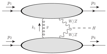
We begin with the discussion of the kinematics of Higgs production in the WBF process

$$q(p_{1})+q(p_{2})\to q(p_{3})+q(p_{4})+H(p_{H})\,.$$ (1)

We perform the Sudakov decomposition of the four-momenta of the outgoing quarks and write

$$\begin{split}&p_{3}=\alpha_{3}p_{1}+\beta_{3}p_{2}+p_{3,\perp}\,,\\ &p_{4}=\alpha_{4}p_{1}+\beta_{4}p_{2}+p_{4,\perp}\,.\end{split}$$ (2)

Employing the on-shell conditions $p^{2}_{3}=0$, $p^{2}_{4}=0$, we find

$$\begin{split}\beta_{3}=\frac{{\bf p}_{3,\perp}^{2}}{s\alpha_{3}}\,,\;\;\;\;\alpha_{4}=\frac{{\bf p}_{4,\perp}^{2}}{s\beta_{4}}\,,\end{split}$$ (3)

where $s=2p_{1}\cdot p_{2}$ is the partonic center-of-mass energy squared. The WBF events are selected by requiring that two tagging jets with a relatively small transverse momentum are present in opposite hemispheres; this ensures that $\alpha_{3}\sim\beta_{4}\sim 1$ and that ${\bf p}_{3,\perp}^{2}\sim{\bf p}_{4,\perp}^{2}\ll s$.

We define two auxiliary vectors $q_{1}$ and $q_{2}$ which describe momentum transfers from the quark lines to the Higgs boson. They read

$$\begin{split}&q_{1}=p_{1}-p_{3}=\delta_{3}p_{1}-\beta_{3}p_{2}-p_{3,\perp}\,,\\ &q_{2}=p_{2}-p_{4}=-\alpha_{4}p_{1}+\delta_{4}p_{2}-p_{4,\perp}\,,\end{split}$$ (4)

where $\delta_{3}=1-\alpha_{3}$ and $\delta_{4}=1-\beta_{4}$. It follows from the momentum conservation condition that

$$p_{H}=q_{1}+q_{2}\,.$$ (5)

Upon squaring the two sides of this equation and some rearrangements, we find

$$\delta_{3}\delta_{4}s=m_{H}^{2}+\frac{{\bf p}_{3,\perp}^{2}}{\alpha_{3}}+\frac{{\bf p}_{4,\perp}^{2}}{\beta_{4}}+2{\bf p}_{3,\perp}\cdot{\bf p}_{4,\perp}-\frac{{\bf p}_{3,\perp}^{2}{\bf p}_{4,\perp}^{2}}{\alpha_{3}\beta_{4}s}\,.$$ (6)

We can use Eq. (6) to fully specify the relevant aspects of WBF kinematics around the forward limit. Indeed, given the proximity of the Higgs boson mass and electroweak boson masses, and the fact that the important contribution to WBF cross section comes from kinematical configurations where the transverse momenta of tagging jets are comparable to $m_{H}$ and $m_{W,Z}$, the above equation implies

$$\delta_{3}\delta_{4}\sim\frac{m_{V}^{2}}{s}\sim\frac{m_{H}^{2}}{s}\sim\frac{{\bf p}_{3,\perp}^{2}}{s}\sim\frac{{\bf p}_{4,\perp}^{2}}{s}\sim\lambda\ll 1\,.$$ (7)

Note that we introduced a parameter $\lambda$ to indicate the smallness of various ratios in the above equation. We consider central production of Higgs bosons so that neither forward nor backward direction is preferred. Then $\delta_{3}\sim\delta_{4}$ and

$$\delta_{3}\sim\delta_{4}\sim\sqrt{\lambda}\gg\lambda\,.$$ (8)

We note that, with the required accuracy, the two parameters $\delta_{3,4}$ can be written as follows

$$\delta_{3,4}=\sqrt{\frac{{\bf p}_{H,\perp}^{2}+m_{H}^{2}}{s}}e^{\pm y_{H}}\,,$$ (9)

where ${\bf p}_{H,\perp}$ is the transverse momentum and $y_{H}$ is the rapidity of the Higgs boson in the partonic center-of-mass frame. We will use the above relations between kinematic parameters to construct the expansion of one- and two-loop non-factorizable WBF amplitudes in the following sections.

3 One-loop non-factorizable contributions to WBF

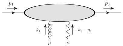
We consider the one-loop non-factorizable QCD corrections to Higgs boson production in WBF. To avoid confusion, we note that they do not contribute to the WBF cross section at NLO since their interference with the leading order amplitude vanishes because of color conservation. Nevertheless, since the one-loop amplitude is needed for the construction of the NNLO QCD corrections, we need to discuss it.

To write the non-factorizable amplitude in a convenient way, we assume that the coupling of the vector boson $V$ to the Higgs boson is given by $ig_{VVH}\;g_{\mu\nu}$ and that the coupling of the massive vector boson to quarks is vector-like, $-ig_{W}\gamma^{\mu}$. Since we work with massless quarks, their helicities are conserved and we can reconstruct non-factorizable contributions for $V=Z$ and $V=W$ from the results that are reported below.

We write the one-loop non-factorizable amplitude as follows

$${\cal M}_{1}=g_{s}^{2}g_{W}^{2}\;g_{VVH}\;T^{a}_{i_{3}i_{1}}T^{a}_{i_{4}i_{2}}\;{\cal A}_{1}\,,$$ (10)

where $T^{a}_{ij}$ denote the generators of the $SU(3)$ color group and ${\cal A}_{1}$ stands for the color-stripped one-loop amplitude

$${\cal A}_{1}=\int\frac{{\rm d}^{d}k_{1}}{(2\pi)^{d}}\frac{1}{d_{1}d_{3}d_{4}}J_{\mu\nu}(k_{1},-k_{1}-q_{1})\;{\tilde{J}}^{\mu\nu}(-k_{1},k_{1}-q_{2})\,.$$ (11)

In Eq. (11), we used the notation

$$d_{1}=k_{1}^{2}+i0,\;\;\;d_{3}=(k_{1}+q_{1})^{2}-m_{V}^{2}+i0,\;\;\;d_{4}=(k_{1}-q_{2})^{2}-m_{V}^{2}+i0\,,$$ (12)

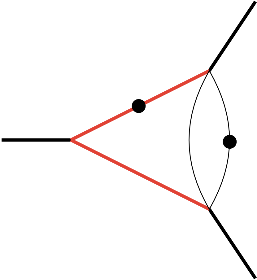
to define propagators of virtual bosons. In addition, following the conventions in Fig. 1, we introduced two quark currents

$$\begin{split}&J^{\mu\nu}(k_{1},-k_{1}-q_{1})=\langle 3|\left[\frac{\gamma^{\nu}(\hat{p}_{1}+\hat{k}_{1})\gamma^{\mu}}{\rho_{1}(k_{1})}+\frac{\gamma^{\mu}(\hat{p}_{3}-\hat{k}_{1})\gamma^{\nu}}{\rho_{3}(-k_{1})}\right]|1]\,,\\ &{\tilde{J}}^{\mu\nu}(-k_{1},k_{1}-q_{2})=\langle 4|\left[\frac{\gamma^{\nu}(\hat{p}_{2}+\hat{k}_{1})\gamma^{\mu}}{\rho_{2}(k_{1})}+\frac{\gamma^{\nu}(\hat{p}_{4}-\hat{k}_{1})\gamma_{\mu}}{\rho_{4}(-k_{1})}\right]|2]\,,\end{split}$$ (13)

where we assumed that the incoming fermions are left-handed. In writing Eq. (13) we employed the quantities $\rho_{i}(k)$, $i=1,2,3,4$ to describe quark propagators; they read

$$\rho_{i}(k)=\frac{1}{(p_{i}+k)^{2}+i0}\,.$$ (14)

We would like to construct an expansion of the amplitude in Eq. (11) in powers of $\lambda$. To understand how to do tatt, we introduce the Sudakov parametrization of the loop momentum $k_{1}$ and write

$$k_{1}=\alpha_{1}p_{1}+\beta_{1}p_{2}+k_{1,\perp}\,.$$ (15)

The integration measure in Eq. (11) becomes

$$\frac{{\rm d}^{d}k_{1}}{(2\pi)^{d}}=\frac{s}{2}\;\frac{{\rm d}\alpha_{1}}{2\pi}\;\frac{{\rm d}\beta_{1}}{2\pi}\frac{{\rm d}^{d-2}{\bf k}_{1,\perp}}{(2\pi)^{d-2}}\,.$$ (16)

Region	$\alpha_{1}$	$\beta_{1}$	${\bf k}_{1,\perp}$
a	$\lambda$	$\lambda$	$\sqrt{\lambda}$
b	$\lambda$	$\sqrt{\lambda}$	$\sqrt{\lambda}$
c	$\sqrt{\lambda}$	$\sqrt{\lambda}$	$\sqrt{\lambda}$
d	$1$	$\lambda$	$\sqrt{\lambda}$
e	$1$	$1$	$1$

Table 1: Kinematic regions relevant for one-loop non-factorizable contributions. Symmetric regions are not shown.

The various propagators in Eq. (11) are linear polynomials in $\alpha_{1}$ and $\beta_{1}$. Hence, integration over either one of these two variables can be easily performed using the residue theorem. The resulting integrand is a product of (at most) quadratic polynomials in the other variable so that the structure of singularities can be easily analyzed. Performing this analysis and assuming that the transverse loop momentum can either be of the same order as the transverse momenta of the outgoing jets or of the same order as the center-of-mass energy, we come to the conclusion that the following loop-momenta regions, shown in Table 1, need to be considered. The first region is the so-called Glauber region; the second one is “Glauber-soft”, the third one is soft, the fourth is collinear and the last one is hard.

Figure 1: The one-loop amplitude, shown on the left, can be constructed by contracting the currents for the upper and lower fermion lines. The current for the upper fermion line $J^{\mu\nu}(k_{1},-k_{1}-q_{1})$ is shown on the right.

Using the scaling of the loop-momentum components as indicated in Table 1, we estimate the contributions of the various regions to the one-loop amplitude. We find

$${\cal M}^{(a)}\sim\lambda^{-2}\,,\;\;\;{\cal M}^{(b)}\sim\lambda^{-2}\,,\;\;\;{\cal M}^{(c)}\sim\lambda^{-2}\,,\;\;\;{\cal M}^{(d)}\sim\lambda^{-3/2}\,,\;\;\;{\cal M}^{(e)}\sim 1\,.$$ (17)

We note that the leading order WBF amplitude scales as $\lambda^{-2}$ and that, as follows from Eq. (17), the expansion of the one-loop amplitude proceeds in powers of $\sqrt{\lambda}$. To compute ${\cal O}(\sqrt{\lambda})$ correction to the virtual amplitude, we need to account for the contributions of regions $a)$, $b)$ and $c)$ to first subleading power and the contribution of region $d)$ to leading power in the expansion in $\lambda$.

We begin with the discussion of region $a)$. Using momentum scaling in Table 1, we simplify the various propagators that appear in the integrand in Eq. (13). To present the result in a compact way, we introduce the following quantities

$$\begin{split}&\Delta_{1}=-{\bf k}_{1,\perp}^{2},\;\;\;\Delta_{3,1}=-({\bf k}_{1,\perp}-{\bf p}_{3,\perp})^{2}-m_{V}^{2},\;\;\;\Delta_{4,1}=-({\bf k}_{1,\perp}+{\bf p}_{4,\perp})^{2}-m_{V}^{2}\,,\\ &\Theta_{3,1}=-\left({\bf k}_{1,\perp}^{2}-2{\bf k}_{1,\perp}\cdot{\bf p}_{3,\perp}\right)\,,\;\;\;\;\;\;\Theta_{4,1}=-\left({\bf k}_{1,\perp}^{2}+2{\bf k}_{1,\perp}\cdot{\bf p}_{4,\perp}\right)\,.\end{split}$$ (18)

In region $a)$, all inverse propagators scale as ${\cal O}(\lambda)$. To compute the first subleading correction we need to keep all terms that scale as $\lambda^{3/2}$ and neglect all terms that scale as $\lambda^{2}$. We find

$$\begin{split}&d_{1}\approx\Delta_{1}+i0,\;\;\;d_{3}\approx s\delta_{3}(\beta_{1}-\beta_{3})+\Delta_{3,1}+i0,\;\;\;d_{4}\approx-s\delta_{4}(\alpha_{1}+\alpha_{4})+\Delta_{4,1}+i0\,,\;\;\\ &\rho_{1}(k_{1})\approx s\beta_{1}+\Delta_{1}+i0\,,\;\;\;\;\;\;\;\;\;\;\;\;\;\rho_{2}(-k_{1})\approx-s\alpha_{1}+\Delta_{1}+i0\,,\\ &\rho_{3}(-k_{1})\approx-s\alpha_{3}\beta_{1}+\Theta_{3,1}+i0\,,\;\;\;\rho_{4}(k_{1})\approx s\beta_{4}\alpha_{1}+\Theta_{4,1}+i0\,.\end{split}$$ (19)

If we use the simplified propagators shown in Eq. (19) to compute the amplitude ${\cal A}_{1}$, we observe that integrations over $\alpha_{1}$ and $\beta_{1}$ factorize. We then write

$${\cal A}_{1}^{(a)}=-\frac{s}{2}\;\int\frac{{\rm d}^{d-2}{\bf k}_{1,\perp}}{(2\pi)^{d-2}}\;\frac{1}{\Delta_{1}\Delta_{3,1}\Delta_{4,1}}\;\Phi^{\mu\nu}\;\tilde{\Phi}_{\mu\nu}\,,$$ (20)

where

$$\begin{split}&\Phi^{\mu\nu}=\int\limits_{-\sigma}^{\sigma}\frac{{\rm d}\beta_{1}}{2\pi i}\frac{\Delta_{3,1}}{s\delta_{3}(\beta_{1}-\beta_{3})+\Delta_{3,1}+i0}\\ &\qquad\qquad\qquad\times\langle 3|\left[\frac{\gamma^{\nu}(\hat{p}_{1}+\hat{k}_{1,\perp})\gamma^{\mu}}{s\beta_{1}+\Delta_{1}+i0}+\frac{\gamma^{\mu}(\hat{p}_{3}-\hat{k}_{1,\perp})\gamma^{\nu}}{-s\alpha_{3}\beta_{1}+\Theta_{3,1}+i0}\right]|1]\,,\end{split}$$ (21)

$$\begin{split}&\tilde{\Phi}^{\mu\nu}=\int\limits_{-\sigma}^{\sigma}\frac{{\rm d}\alpha_{1}}{2\pi i}\frac{\Delta_{4,1}}{-s\delta_{4}(\alpha_{1}+\alpha_{4})+\Delta_{4,1}+i0}\\ &\qquad\qquad\qquad\times\langle 4|\left[\frac{\gamma^{\nu}(p_{2}+\hat{k}_{1,\perp})\gamma^{\mu}}{-s\alpha_{1}+\Delta_{1}+i0}+\frac{\gamma^{\nu}(p_{4}-\hat{k}_{1,\perp})\gamma^{\mu}}{s\beta_{4}\alpha_{1}+\Theta_{4,1}+i0}\right]|2]\,.\end{split}$$ (22)

In Eq. (20) $\sigma$ is a cut-off parameter that forces $\beta_{1}$ and $\alpha_{1}$ to stay in the region $\alpha_{1}\sim\beta_{1}\sim\lambda$. It is convenient to choose $\sigma$ such that

$$\lambda\ll\sigma\ll\sqrt{\lambda}\,,$$ (23)

since this choice will allow us to use the same cut-off $\sigma$ to study the Glauber-soft region.

We note that we replaced $\hat{k}_{1}$ with $\hat{k}_{1,\perp}$ in the currents when writing Eq. (20); this is justified since $\alpha_{1}$ and $\beta_{1}$ terms in the Sudakov expansion of $k$ provide ${\cal O}(\lambda)$ and not ${\cal O}(\sqrt{\lambda})$ corrections in region $a)$. Hence, if we aim at computing the non-factorizable amplitude with ${\cal O}(\sqrt{\lambda})$ relative accuracy, we can discard them. In fact, to compute the amplitude with ${\cal O}(\sqrt{\lambda})$ relative accuracy, terms with $\hat{k}_{1,\perp}$ in Eq. (20) can be dropped altogether. Indeed, since $k_{1,\perp}\sim\sqrt{\lambda}$, if we retain it in one of the terms that appear either in $\Phi^{\mu\nu}$ or in $\tilde{\Phi}^{\mu\nu}$, the other current should be computed at leading $\lambda$-power. However, in this case

$$\langle 4|\gamma^{\mu}\hat{p}_{2,4}\gamma^{\nu}|2]\approx 4p_{2}^{\mu}p_{2}^{\nu}\,,\;\;\;\;\;\;\langle 3|\gamma^{\mu}\hat{p}_{3,1}\gamma^{\nu}|1]\approx 4p_{1}^{\mu}p_{1}^{\nu}\,,\;\;\;\;\;$$ (24)

and terms with $\hat{k}_{1,\perp}$ lead to the vanishing contributions

$$\hat{p}_{i}\;\hat{k}_{1,\perp}\;\hat{p}_{i}=0,\;\;\;i=1,2\,,$$ (25)

since $p_{1,2}^{2}=0$ and $p_{1,2}\cdot k_{1,\perp}=0$.

Furthermore, in region $a)$ we can expand the remnants of weak boson propagators that appear in Eq. (20). Keeping terms that provide ${\cal O}(\sqrt{\lambda})$ corrections, we find

$$\begin{split}&\frac{\Delta_{3,1}}{s\delta_{3}(\beta_{1}-\beta_{3})+\Delta_{3,1}+i0}\approx 1+\frac{s\delta_{3}(\beta_{3}-\beta_{1})}{\Delta_{3,1}}+{\cal O}(\lambda)\,,\\ &\frac{\Delta_{4,1}}{-s\delta_{4}(\alpha_{1}+\alpha_{4})+\Delta_{4,1}+i0}\approx 1+\frac{s\delta_{4}(\alpha_{4}+\alpha_{1})}{\Delta_{4,1}}+{\cal O}(\lambda)\,.\end{split}$$ (26)

Focusing on $\Phi^{\mu\nu}$, we simplify the expression for the current, use Eq. (26) and obtain

$$\Phi^{\mu\nu}=\frac{2p_{1}^{\mu}\langle 3|\gamma^{\nu}|1]}{s}\;\Phi\,,$$ (27)

where

$$\begin{split}\Phi=\int\limits_{-\sigma}^{\sigma}\frac{{\rm d}\beta_{1}}{2\pi i}\left(1+\frac{s\delta_{3}(\beta_{3}-\beta_{1})}{\Delta_{3,1}}\right)&\Bigg{[}\frac{1}{\beta_{1}+\frac{\Delta_{1}}{s}+i0}+\frac{1}{-\beta_{1}+\frac{\Theta_{3,1}}{s\alpha_{3}}+i0}\Bigg{]}\,.\end{split}$$ (28)

To compute $\Phi$, we use

$$\int\limits_{-\sigma}^{\sigma}\frac{{\rm d}\beta_{1}}{2\pi i}\;\frac{1}{\pm\beta_{1}-z_{a}+i0}=-\frac{1}{2}+{\cal O}(z_{a}/\sigma)\,,$$ (29)

valid for $z_{a}\in[-\sigma,\sigma]$. Furthermore, we need

$$\int_{-\sigma}^{\sigma}\frac{{\rm d}\beta_{1}}{2\pi i}\;\beta_{1}\;\left(\frac{1}{\beta_{1}-z_{a}+i0}+\frac{1}{-\beta_{1}-z_{b}+i0}\right)=-\frac{1}{2}\left(z_{a}-z_{b}\right)+{\cal O}(z_{a}^{2}/\sigma,z_{b}^{2}/\sigma)\,.$$ (30)

Neglecting the $\sigma$-dependent terms that will cancel with the contribution from the Glauber-soft region, we obtain

$$\Phi=(-1)\left[1+\frac{\delta_{3}}{2\Delta_{3,1}}\left(2s\beta_{3}+\Delta_{1}-\Theta_{3,1}\right)\right]\,.$$ (31)

A similar computation for $\tilde{\Phi}^{\mu\nu}$ gives

$$\tilde{\Phi}^{\mu\nu}=\frac{2p_{2}^{\mu}\langle 4|\gamma^{\nu}|2]}{s}\tilde{\Phi}\,,$$ (32)

where

$$\tilde{\Phi}=(-1)\left[1+\frac{\delta_{4}}{2\Delta_{4,1}}\left(2s\beta_{4}+\Delta_{1}-\Theta_{4,1}\right)\right]\,.$$ (33)

Combining these results for $\Phi$ and $\tilde{\Phi}$ and neglecting all terms beyond desired ${\cal O}(\sqrt{\lambda})$ corrections, we obtain the following contribution to the one-loop amplitude from the Glauber region

$$\begin{split}{\cal A}_{1}^{(a)}&=-\langle 3|\gamma^{\mu}|1]\langle 4|\gamma_{\mu}|2]\;\int\frac{{\rm d}^{d-2}{\bf k}_{1,\perp}}{(2\pi)^{d-2}}\;\frac{1}{\Delta_{1}\Delta_{3,1}\Delta_{4,1}}\\ &\times\left(1+\frac{\delta_{3}}{2\Delta_{3,1}}\left(2s\beta_{3}+\Delta_{1}-\Theta_{3,1}\right)+\frac{\delta_{4}}{2\Delta_{4,1}}\left(2s\beta_{4}+\Delta_{1}-\Theta_{4,1}\right)\right)\,.\end{split}$$ (34)

We then proceed with the discussion of the contribution of region $b)$ with the mixed scaling $\alpha_{1}\sim\lambda$ and $\beta_{1}\sim\sqrt{\lambda}$. According to Eq. (17), we require the contribution of this region through first subleading terms. However, it is easy to see that, in actuality, the contribution of region $b)$ starts at ${\cal O}(\lambda^{-3/2})$ and, therefore, should be computed at leading power only.

To understand why this is the case, we first discuss the currents $J^{\mu\nu}$ and ${\tilde{J}}^{\mu\nu}$ and, in particular, the numerators of the contributing terms. Since we work with ${\cal O}(\sqrt{\lambda})$ accuracy, in region $b)$ we should replace $k_{1}$ with $k_{1}\to\beta_{1}p_{2}+k_{1,\perp}$ in both currents. Suppose we do this replacement in $J^{\mu\nu}$. Since these terms already provide an ${\cal O}(\sqrt{\lambda})$ correction, the current ${\tilde{J}}^{\mu\nu}$ should be taken at leading power. Since at leading power ${\tilde{J}}^{\mu\nu}\sim p_{2}^{\mu}p_{2}^{\nu}$, it is easy to see that all contributions of vector $k_{1}$ drop from the current $J^{\mu\nu}$ once the Lorentz indices are contracted.

However, if we account for $k_{1}$ in the current ${\tilde{J}}^{\mu\nu}$, the situation is different. In this case, since $i)$ $k_{1}$ is independent of $\alpha_{1}$, $ii)$ it appears with different signs in the two terms in ${\tilde{J}}^{\mu\nu}$, and $iii)$ ${\tilde{J}}^{\mu\nu}$ is contracted with ${J}^{\mu\nu}$ computed at leading power, the corresponding contribution vanishes after integration over $\alpha_{1}$.

Having concluded that, similar to the Glauber region, we can drop $k_{1}$ from the fermion currents, we note that the current $J^{\mu\nu}(k_{1},-q_{1}-k_{1})$ in region $b)$ can be further simplified. Indeed, using the fact that $\beta_{1}\gg\Delta_{1}/s,\Theta_{3,1}/s$, we expand the current and obtain

$$\begin{split}J^{\mu\nu}(k_{1},-q_{1}-k_{1})&\approx p_{1}^{\mu}p_{1}^{\nu}\left(\frac{1}{s\beta_{1}+\Delta_{1}+i0}+\frac{\alpha_{3}}{-s\alpha_{3}\beta_{1}+\Theta_{3,1}+i0}\right)\\ &\approx-\frac{p_{1}^{\mu}p_{1}^{\nu}}{s\beta_{1}^{2}}\left(\Delta_{1}+\Theta_{3,1}\right)\,.\end{split}$$ (35)

This equation implies that in region $b)$ the current scales as ${\cal O}(1)$ and not as ${\cal O}(\lambda^{-1/2})$ as a naive estimate suggests. This suppression occurs because of the cancellation between two terms in brackets in Eq. (35). This means that the contribution of the region $b)$ starts at $\lambda^{-3/2}$, so that all ingredients needed to compute the amplitude in region $b)$, except the current $J^{\mu\nu}(k_{1},-q_{1}-k_{1})$, are to be taken at leading power in $\lambda$.

Hence, we find

$${\cal A}_{1}^{(b)}=-\langle 3|\gamma_{\mu}|1]\langle 4|\gamma^{\mu}|2]\int\frac{{\rm d}^{d-2}{\bf k}_{1,\perp}}{(2\pi)^{d-2}}\;\frac{1}{\Delta_{1}\Delta_{3,1}\Delta_{4,1}}\;\Delta\Phi\;\tilde{\Phi},$$ (36)

where $\tilde{\Phi}$ is still given by Eq. (33) and

$$\Delta\Phi=\left(-\frac{\Delta_{1}}{s}-\frac{\Theta_{3,1}}{s}\right)\int\limits_{-\infty}^{\infty}\frac{{\rm d}\beta_{1}}{2\pi i}\frac{(\theta(\beta_{1}-\sigma)+\theta(-\sigma-\beta_{1}))\Delta_{3,1}}{(s\delta_{3}\beta_{1}+\Delta_{3,1}+i0)\;\beta_{1}^{2}}\,.$$ (37)

Calculation of this integral is straightforward. We obtain

$$\Delta\Phi=\frac{\delta_{3}}{2\Delta_{3,1}}\left(\Delta_{1}+\Theta_{3,1}\right)\,.$$ (38)

Performing a similar computation for a symmetric region $\beta\sim\lambda,\;\alpha\sim\sqrt{\lambda}$, we obtain

$$\Delta\tilde{\Phi}=\frac{\delta_{4}}{2\Delta_{4,1}}\left(\Delta_{1}+\Theta_{4,1}\right)\,.$$ (39)

Combining the contributions of regions $a)$ and $b)$, we find

$$\begin{split}{\cal A}_{1}^{a\&b}&=-\langle 3|\gamma^{\mu}|1]\langle 4|\gamma_{\mu}|2]\;\int\frac{{\rm d}^{d-2}{\bf k}_{1,\perp}}{(2\pi)^{d-2}}\;\frac{1}{\Delta_{1}\Delta_{3,1}\Delta_{4,1}}\\ &\times\left(1+\frac{\delta_{3}}{\Delta_{3,1}}\left(s\beta_{3}-\Theta_{3,1}\right)+\frac{\delta_{4}}{\Delta_{4,1}}\left(s\alpha_{4}-\Theta_{4,1}\right)\right)\,.\end{split}$$ (40)

We turn our attention to region $c)$ which corresponds to the soft scaling $\alpha_{1}\sim\beta_{1}\sim|{\bf k}_{1,\perp}|\sim\sqrt{\lambda}$. According to Eq. (17) we require the contribution of this region through first subleading power. However, a more careful analysis shows that the contribution of this region is suppressed stronger than originally expected. To see this we note that in the soft region, to leading power, the currents vanish. For example, the expression for $J^{\mu\nu}(k_{1},-q_{1}-k_{1})$ reads

$$J^{\mu\nu}(k_{1},-q_{1}-k_{1})\approx p_{1}^{\mu}p_{1}^{\nu}\left(\frac{1}{s\beta_{1}+i0}+\frac{\alpha_{3}}{-s\alpha_{3}\beta_{1}+i0}\right)=p_{1}^{\mu}p_{1}^{\nu}(-2i\pi)\delta(\beta_{1})\to 0\,,$$ (41)

and we have set it to zero because poles of the fermion propagators have already been accounted for when the Glauber region was analyzed. Hence, to obtain a non-vanishing contribution from the soft region, subleading terms in both currents $J^{\mu\nu}$ and ${\tilde{J}}^{\mu\nu}$ are needed. The subleading contributions to the currents scale as ${\cal O}(1)$ and not as $1/\sqrt{\lambda}$ as a naive estimate for the currents’ scaling would suggest. This implies that at variance with the original estimate ${\cal M}^{(c)}\sim\lambda^{-2}$ in Eq. (17), the contribution of the soft region is suppressed by an additional power of $\lambda$. For this reason, the soft region is not needed for computing the two-loop non-factorizable amplitude with ${\cal O}(\sqrt{\lambda})$ accuracy.

The contribution of the collinear region can be analyzed in the same way. Since, in this case, the amplitude scales as ${\cal M}^{d}\sim\lambda^{-3/2}$, both currents need to be taken at leading power. We find

$$\begin{split}&J^{\mu\nu}(k_{1},k_{2})=\langle 3|\left[\frac{\gamma^{\nu}(\hat{p}_{1}+\beta_{1}\hat{p}_{2})\gamma^{\mu}}{\beta_{1}s+i0}+\frac{\gamma^{\mu}(\hat{p}_{1}-\beta_{1}\hat{p}_{2})\gamma^{\nu}}{-\beta_{1}s+i0}\right]|1]\\ &=\langle 3|\gamma^{\mu}\hat{p}_{2}\gamma^{\nu}+\gamma^{\nu}\hat{p}_{2}\gamma^{\mu}|1]=2\langle 3|p_{2}^{\mu}\gamma^{\nu}+p_{2}^{\nu}\gamma^{\mu}-g^{\mu\nu}\hat{p}_{2}|1],\\ &{\tilde{J}}^{\mu\nu}(k_{1},k_{2})=\langle 4|\left[(1+\beta_{1})\frac{\gamma^{\nu}\hat{p}_{2}\gamma^{\mu}}{\rho_{2}(k_{1})}+(1-\beta_{1})\frac{\gamma^{\nu}\hat{p}_{2}\gamma^{\mu}}{\rho_{4}(-k_{1})}\right]|2]\,.\end{split}$$ (42)

It is clear that the contraction of the two currents in Eq. (42) vanishes. Hence, we conclude that collinear regions do not provide the ${\cal O}(\sqrt{\lambda})$ corrections to the leading term in the eikonal expansion. Since, obviously, the hard region is not relevant as well, we conclude that, with ${\cal O}(\sqrt{\lambda})$ accuracy, the one-loop non-factorizable contribution is given by the sum of the Glauber and Glauber-soft contributions in Eq. (40).

Having performed this analysis, we note that the final result for the two regions $a)$ and $b)$ can be obtained by simply computing the functions $\Phi$ and $\tilde{\Phi}$ from the following unexpanded expressions

$$\begin{split}&\Phi=\int\frac{{\rm d}\beta_{1}}{2\pi i}\frac{\Delta_{3,1}}{s\delta_{3}(\beta_{1}-\beta_{3})+\Delta_{3,1}+i0}\Bigg{[}\frac{1}{\beta_{1}+\frac{\Delta_{1}}{s}+i0}+\frac{1}{-\beta_{1}+\frac{\Theta_{3,1}}{s\alpha_{3}}+i0}\Bigg{]}\,,\\ &\tilde{\Phi}=\int\frac{{\rm d}\alpha_{1}}{2\pi i}\frac{\Delta_{4,1}}{-s\delta_{4}(\alpha_{1}+\alpha_{4})+\Delta_{4,1}+i0}\Bigg{[}\frac{1}{-\alpha_{1}+\frac{\Delta_{1}}{s}+i0}+\frac{1}{\alpha_{1}+\frac{\Theta_{4,1}}{s\beta_{4}}+i0}\Bigg{]}\;.\end{split}$$ (43)

It is straightforward to integrate over $\beta_{1}$ and $\alpha_{1}$ in Eq. (43). Indeed, focusing on the function $\Phi$, we note that, if we close the integration contour in the upper half plane, only the residue at $\beta_{1}=\Theta_{3,1}/(s\alpha_{3})$ contributes. We then find

$$\Phi=(-1)\frac{\Delta_{3,1}}{\Delta_{3,1}+\delta_{3}(\Theta_{3,1}-s\beta_{3})}\,.$$ (44)

Expanding this result in $\delta_{3}$, performing a similar computation for $\tilde{\Phi}$, and keeping only the relevant terms in the product of $\Phi$ and $\tilde{\Phi}$, we obtain Eq. (40).

Finally, it is convenient to write the one-loop non-factorizable amplitude by extracting exact (i.e. not expanded in powers of $\lambda$) Born amplitude. The latter reads

$${\cal M}_{0}=ig_{W}^{2}\;g_{VVH}\frac{\langle 3|\gamma^{\mu}|1]\langle 4|\gamma_{\mu}|2]}{(q_{1}^{2}-m_{V}^{2})(q_{2}^{2}-m_{V}^{2})}.$$ (45)

Using it, we write

$${\cal M}_{1}=i\frac{g_{s}^{2}}{4\pi}\;T^{a}_{i_{3}i_{1}}T^{a}_{i_{4}i_{2}}\,{\cal M}_{0}\,{\cal C}_{1},$$ (46)

The function $C_{1}$ reads

$$\begin{split}{\cal C}_{1}=2\int&\frac{{\rm d}^{d-2}{\bf k}_{1,\perp}}{(2\pi)^{1-2\epsilon}}\frac{({\bf p}_{3,\perp}^{2}+m_{V}^{2})({\bf p}_{4,\perp}^{2}+m_{V}^{2})}{\Delta_{1}\Delta_{3,1}\Delta_{4,1}}\\ &\times\left[1-\delta_{3}\left(\frac{m_{V}^{2}}{{\bf p}_{3,\perp}^{2}+m_{V}^{2}}+\frac{m_{V}^{2}}{\Delta_{3,1}}\right)-\delta_{4}\left(\frac{m_{V}^{2}}{{\bf p}_{4,\perp}^{2}+m_{V}^{2}}+\frac{m_{V}^{2}}{\Delta_{4,1}}\right)\right].\end{split}$$ (47)

We note that the above expression includes both the leading and the first subleading terms in the expansion of the one-loop amplitude in powers of $\sqrt{\lambda}$. The function ${\cal C}_{1}$ can be computed analytically and expressed through logarithmic and dilogarithmic functions; the corresponding discussion can be found in appendix.

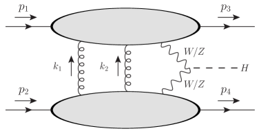
4 Two-loop non-factorizable contributions to WBF

We continue with the computation of two-loop non-factorizable QCD corrections to Higgs boson production in weak boson fusion. The two-loop non-factorizable amplitude is written as

$${\cal M}_{2}=-ig_{s}^{4}g_{W}^{2}g_{VVH}\left(\frac{1}{2}\{T^{a},T^{b}\}\right)_{i_{3}i_{1}}\left(\frac{1}{2}\{T^{a},T^{b}\}\right)_{i_{4}i_{2}}{\cal A}_{2}\,,$$ (48)

where

$${\cal A}_{2}=\frac{1}{2!}\int\frac{{\rm d}^{d}k_{1}}{(2\pi)^{d}}\frac{{\rm d}^{d}k_{2}}{(2\pi)^{d}}\frac{1}{d_{1}d_{2}d_{3}d_{4}}J_{\mu\nu\alpha}(k_{1},k_{2},-k_{12}-q_{1}){\tilde{J}}^{\mu\nu\alpha}(-k_{1},-k_{2},k_{12}-q_{2})\,.$$ (49)

The overall factor $1/2!$ comes from the symmetrization of two identical gluons and

$$d_{1}=k_{1}^{2}+i0,\;\;d_{2}=k_{2}^{2}+i0,\;\;\;d_{3}=(k_{12}+q_{1})^{2}-m_{V}^{2}+i0,\;\;\;d_{4}=(k_{12}-q_{2})^{2}-m_{V}^{2}+i0\,,$$ (50)

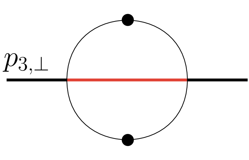
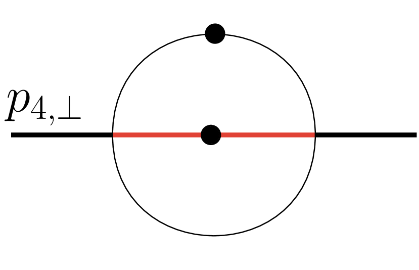
are bosonic propagators. Similarly to the one-loop case, in Eq. (49), we defined two quark currents; the conventions are explained in Fig. 2. The currents read

$$\begin{split}&J^{\mu\nu\alpha}(k_{1},k_{2},-k_{12}-q_{1})=\langle 3|\Bigg{\{}\\ &\frac{\gamma^{\alpha}(\hat{p}_{1}+\hat{k}_{12})\gamma^{\nu}(\hat{p}_{1}+\hat{k}_{1})\gamma^{\mu}}{\rho_{1}(k_{12})\rho_{1}(k_{1})}+\frac{\gamma^{\alpha}(\hat{p}_{1}+\hat{k}_{12})\gamma^{\mu}(\hat{p}_{1}+\hat{k}_{2})\gamma^{\nu}}{\rho_{1}(k_{12})\rho_{1}(k_{2})}\\ &+\frac{\gamma^{\nu}(\hat{p}_{3}-\hat{k}_{2})\gamma^{\alpha}(\hat{p}_{1}+\hat{k}_{1})\gamma^{\mu}}{\rho_{3}(-k_{2})\rho_{1}(k_{1})}+\frac{\gamma^{\mu}(\hat{p}_{3}-\hat{k}_{1})\gamma^{\alpha}(\hat{p}_{1}+\hat{k}_{2})\gamma^{\nu}}{\rho_{3}(-k_{1})\rho_{1}(k_{2})}\\ &+\frac{\gamma^{\nu}(\hat{p}_{3}-\hat{k}_{2})\gamma^{\mu}(\hat{p}_{3}-\hat{k}_{12})\gamma^{\alpha}}{\rho_{3}(-k_{2})\rho_{3}(-k_{12})}+\frac{\gamma^{\mu}(\hat{p}_{3}-\hat{k}_{1})\gamma^{\nu}(\hat{p}_{3}-\hat{k}_{12})\gamma^{\alpha}}{\rho_{3}(-k_{1})\rho_{3}(-k_{12})}\Bigg{\}}|1]\,,\end{split}$$ (51)

and

$$\begin{split}&{\tilde{J}}^{\mu\nu\alpha}(-k_{1},-k_{2},k_{12}-q_{2})=\langle 4|\Bigg{\{}\\ &\frac{\gamma^{\alpha}(\hat{p}_{2}-\hat{k}_{12})\gamma^{\nu}(\hat{p}_{2}-\hat{k}_{1})\gamma^{\mu}}{\rho_{2}(-k_{12})\rho_{2}(-k_{1})}+\frac{\gamma^{\alpha}(\hat{p}_{2}-\hat{k}_{12})\gamma^{\mu}(\hat{p}_{2}-\hat{k}_{2})\gamma^{\nu}}{\rho_{2}(-k_{12})\rho_{2}(-k_{2})}\\ &+\frac{\gamma^{\nu}(\hat{p}_{4}+\hat{k}_{2})\gamma^{\alpha}(\hat{p}_{2}-\hat{k}_{1})\gamma^{\mu}}{\rho_{4}(k_{2})\rho_{2}(-k_{1})}+\frac{\gamma^{\mu}(\hat{p}_{4}+\hat{k}_{1})\gamma^{\alpha}(\hat{p}_{2}-\hat{k}_{2})\gamma^{\nu}}{\rho_{4}(k_{1})\rho_{2}(-k_{2})}\\ &+\frac{\gamma^{\nu}(\hat{p}_{4}+\hat{k}_{2})\gamma^{\mu}(\hat{p}_{4}+\hat{k}_{12})\gamma^{\alpha}}{\rho_{4}(k_{2})\rho_{4}(k_{12})}+\frac{\gamma^{\mu}(\hat{p}_{4}+\hat{k}_{1})\gamma^{\nu}(\hat{p}_{4}+\hat{k}_{12})\gamma^{\alpha}}{\rho_{4}(k_{1})\rho_{4}(k_{12})}\Bigg{\}}|2]\,.\end{split}$$ (52)

Figure 2: The two-loop amplitude, shown on the left, is thought in terms of the currents that make it up. On the right, we define of the generalized upper current $J^{\mu\nu\alpha}(k_{1},k_{2},-k_{12}-q_{1})$ used in the calculation of the two-loop amplitude.

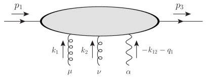
To integrate over the loop momenta $k_{1,2}$, for each of them (and also for their linear combinations) we need to consider regions shown in Table 1. We write

$$k_{i}=\alpha_{i}p_{1}+\beta_{i}p_{2}+k_{i,\perp},\;\;\;i=1,2\,.$$ (53)

The leading contribution comes from the Glauber region where $\alpha_{1}\sim\beta_{1}\sim\alpha_{2}\sim\beta_{2}\sim\lambda$ and $|{\bf k}_{1,\perp}|\sim|{\bf k}_{2,\perp}|\sim\sqrt{\lambda}$. Similar to the one-loop case, the leading correction arises from the mixed region where some of the $\alpha$- or $\beta$-components scale as $\sqrt{\lambda}$. Both in the Glauber region and in the mixed region, the loop momenta in the numerators of both currents $J^{\mu\nu\alpha}$ and ${\tilde{J}}^{\mu\nu\alpha}$ can be discarded. The reason for this is the same as in the one-loop case and we do not repeat this analysis here.

Building on the experience with the one-loop calculation reported in the previous section, we can make the following observation. To obtain ${\cal O}(\sqrt{\lambda})$ correction, we only need to consider the cases where $i)$ one or both $\beta_{1,2}$ components of the loop momenta scale as $\sqrt{\lambda}$ and both $\alpha_{1,2}$ scale as $\lambda$, or $ii)$ the other way around. If one of the two $\alpha$’s and one of the two $\beta$’s scale as $\sqrt{\lambda}$, then $\alpha_{12}$ and $\beta_{12}$ also scale as $\sqrt{\lambda}$. As the result, both currents in Eq. (51) and Eq. (52) are suppressed by $\mathcal{O}(\sqrt{\lambda})$. Thus, the contribution of this region is suppressed by ${\cal O}(\lambda)$ and can be discarded. We conclude that, if we want to construct an integrand which is valid both in the Glauber region and in the mixed region, we need to write an expression that incorporates $\sqrt{\lambda}$ corrections to one of the currents and that the other current should be taken at leading order.

These considerations also guide the expansion of the propagators in powers of $\lambda$ to make them valid in both the Glauber region and in the mixed region. To write the approximate expressions, we define

$$\begin{split}&\Delta_{i}=-{\bf k}_{i,\perp}^{2}\,,\;\;\;\Delta_{3,i}=-({\bf k}_{i,\perp}-{\bf p}_{3,\perp})^{2}-m_{V}^{2}\,,\;\;\;\;\Delta_{4,i}=-({\bf k}_{i,\perp}+{\bf p}_{4,\perp})^{2}-m_{V}^{2}\,,\\ &\Theta_{3,i}=-\left({\bf k}_{i,\perp}^{2}-2{\bf k}_{i,\perp}\cdot{\bf p}_{3,\perp}\right)\,,\;\;\;\Theta_{4,i}=-\left({\bf k}_{i,\perp}^{2}+2{\bf k}_{i,\perp}\cdot{\bf p}_{4,\perp}\right)\,,\end{split}$$ (54)

for $i\in\{1,2,12\}$, where $\alpha_{12}=\alpha_{1}+\alpha_{2}$, $\beta_{12}=\beta_{1}+\beta_{2}$ etc. and obtain

$$d_{1,2}\approx\Delta_{1,2}+i0\,,\;\;\;d_{3}\approx s\delta_{3}(\beta_{12}-\beta_{3})+\Delta_{3,12}+i0\,,\;\;\;$$

$$d_{4}\approx-s\delta_{4}(\alpha_{12}+\alpha_{4})+\Delta_{4,12}+i0\,,\;\;$$

$$\rho_{1}(k_{i})\approx s\beta_{i}+\Delta_{i}+i0\,,\;\;\;\rho_{3}(k_{i})\approx s\alpha_{3}\beta_{3}+\Theta_{3,i}+i0\,,$$ (55)

$$\rho_{2}(k_{i})\approx s\alpha_{i}+\Delta_{i}+i0\,,\;\;\;\rho_{4}(k_{i})\approx s\beta_{4}\alpha_{i}+\Theta_{4,i}+i0\,.$$

We emphasize that the above expressions for propagators are valid both in the Glauber region and in the mixed region. Because of that, we can use them to compute the two-loop non-factorizable amplitude with ${\cal O}(\sqrt{\lambda})$ accuracy in the same way as Eq. (43) was used to do that in the one-loop case.

Using the expanded propagators, we simplify the currents in Eq. (52) and write the amplitude as

$${\cal A}_{2}^{a\&b}=\frac{1}{2!}\langle 3|\gamma^{\alpha}|1]\langle 4|\gamma_{\alpha}|2]\int\frac{{\rm d}^{d-2}{\bf k}_{1,\perp}}{(2\pi)^{d-2}}\;\frac{{\rm d}^{d-2}{\bf k}_{2,\perp}}{(2\pi)^{d-2}}\frac{1}{\Delta_{1}\Delta_{2}\Delta_{3,12}\Delta_{4,12}}\;\Phi\;\tilde{\Phi}\,,$$ (56)

where

$$\begin{split}&\Phi=\int\frac{{\rm d}\beta_{1}}{2\pi i}\frac{{\rm d}\beta_{2}}{2\pi i}\frac{\Delta_{3,12}}{s\delta_{3}(\beta_{12}-\beta_{3})+\Delta_{3,12}+i0}\Bigg{\{}\frac{1}{(\beta_{12}+\frac{\Delta_{12}}{s}+i0)(\beta_{1}+\frac{\Delta_{1}}{s}+i0)}\\ &+\frac{1}{(\beta_{12}+\frac{\Delta_{12}}{s}+i0)(\beta_{2}+\frac{\Delta_{2}}{s}+i0)}+\frac{1}{(-\beta_{2}+\frac{\Theta_{3,2}}{s\alpha_{3}}+i0)(\beta_{1}+\frac{\Delta_{1}}{s}+i0)}\\ &+\frac{1}{(-\beta_{1}+\frac{\Theta_{3,1}}{s\alpha_{3}}+i0)(\beta_{2}+\frac{\Delta_{2}}{s}+i0)}+\frac{1}{(-\beta_{2}+\frac{\Theta_{3,2}}{s\alpha_{3}}+i0)(-\beta_{12}+\frac{\Theta_{3,12}}{s\alpha_{3}}+i0)}\\ &+\frac{1}{(-\beta_{1}+\frac{\Theta_{3,1}}{s\alpha_{3}}+i0)(-\beta_{12}+\frac{\Theta_{3,12}}{s\alpha_{3}}+i0)}\Bigg{\}}\,,\end{split}$$ (57)

and

$$\begin{split}&\tilde{\Phi}=\int\frac{{\rm d}\alpha_{1}}{2\pi i}\frac{{\rm d}\alpha_{2}}{2\pi i}\frac{\Delta_{4,12}}{-s\delta_{4}(\alpha_{4}+\alpha_{12})+\Delta_{4,12}+i0}\Bigg{\{}\frac{1}{(-\alpha_{12}+\frac{\Delta_{12}}{s}+i0)(-\alpha_{1}+\frac{\Delta_{1}}{s}+i0)}\\ &+\frac{1}{(-\alpha_{12}+\frac{\Delta_{12}}{s}+i0)(-\alpha_{2}+\frac{\Delta_{2}}{s}+i0)}+\frac{1}{(\alpha_{2}+\frac{\Theta_{4,2}}{s\beta_{4}}+i0)(-\alpha_{1}+\frac{\Delta_{1}}{s}+i0)}\\ &+\frac{1}{(\alpha_{1}+\frac{\Theta_{4,1}}{s\beta_{4}}+i0)(-\alpha_{2}+\frac{\Delta_{2}}{s}+i0)}+\frac{1}{(\alpha_{2}+\frac{\Theta_{4,2}}{s\beta_{4}}+i0)(\alpha_{12}+\frac{\Theta_{4,12}}{s\beta_{4}}+i0)}\\ &+\frac{1}{(\alpha_{1}+\frac{\Theta_{4,1}}{s\beta_{4}}+i0)(\alpha_{12}+\frac{\Theta_{4,12}}{s\beta_{4}}+i0)}\Bigg{\}}\,.\end{split}$$ (58)

To integrate over $\beta_{1,2}$ and $\alpha_{1,2}$ it is useful to rearrange terms in the curly brackets in Eqs. (57, 58). Focusing on the integrand in Eq. (57), we rewrite it as follows

$$\begin{split}&\Bigg{\{}....\Bigg{\}}\to\frac{\frac{\Delta_{1}}{s}+\frac{\Delta_{2}}{s}-\frac{\Delta_{12}}{s}}{(\beta_{12}+\frac{\Delta_{12}}{s}+i0)(\beta_{1}+\frac{\Delta_{1}}{s}+i0)(\beta_{2}+\frac{\Delta_{2}}{s}+i0)}\\ +&\frac{\frac{\Theta_{3,1}}{\alpha_{3}s}+\frac{\Theta_{3,2}}{\alpha_{3}s}-\frac{\Theta_{3,12}}{\alpha_{3}s}}{(-\beta_{12}+\frac{\Theta_{3,12}}{\alpha_{3}s}+i0)(-\beta_{1}+\frac{\Theta_{3,1}}{\alpha_{3}s}+i0)(-\beta_{2}+\frac{\Theta_{3,2}}{\alpha_{3}s}+i0)}\\ +&\left(\frac{1}{\beta_{1}+\frac{\Delta_{1}}{s}+i0}+\frac{1}{-\beta_{1}+\frac{\Theta_{3,1}}{s\alpha_{3}}+i0}\right)\!\!\left(\frac{1}{\beta_{2}+\frac{\Delta_{2}}{s}+i0}+\frac{1}{-\beta_{2}+\frac{\Theta_{3,2}}{s\alpha_{3}}+i0}\right)\,.\end{split}$$ (59)

We use the above representation to compute the function $\Phi$ in Eq. (57). We note that the first term in Eq. (59) can be discarded, because of the location of its poles. Indeed,

$$\begin{split}\Phi_{1}&=\int\frac{{\rm d}\beta_{1}}{2\pi i}\frac{{\rm d}\beta_{2}}{2\pi i}\frac{\Delta_{3,12}}{s\delta_{3}(\beta_{12}-\beta_{3})+\Delta_{3,12}+i0}\\ &\times\frac{\frac{\Delta_{1}}{s}+\frac{\Delta_{2}}{s}-\frac{\Delta_{12}}{s}}{(\beta_{12}+\frac{\Delta_{12}}{s}+i0)(\beta_{1}+\frac{\Delta_{1}}{s}+i0)(\beta_{2}+\frac{\Delta_{2}}{s}+i0)}=0\,.\end{split}$$ (60)

To compute the contribution of the second term in Eq. (59), we close the integration contours in the lower half-planes for both integration variables. We obtain

$$\begin{split}\Phi_{2}&=\int\frac{{\rm d}\beta_{1}}{2\pi i}\frac{{\rm d}\beta_{2}}{2\pi i}\frac{\Delta_{3,12}}{s\delta_{3}(\beta_{12}-\beta_{3})+\Delta_{3,12}+i0}\\ &\times\frac{\frac{\Theta_{3,1}}{\alpha_{3}s}+\frac{\Theta_{3,2}}{\alpha_{3}s}-\frac{\Theta_{3,12}}{\alpha_{3}s}}{(-\beta_{12}+\frac{\Theta_{3,12}}{\alpha_{3}s}+i0)(-\beta_{1}+\frac{\Theta_{3,_{1}}}{\alpha_{3}s}+i0)(-\beta_{2}+\frac{\Theta_{3,2}}{\alpha_{3}s}+i0)}\\ &=\frac{\delta_{3}(\Theta_{3,1}+\Theta_{3,2}-\Theta_{3,12})}{\Delta_{3,12}}\,.\end{split}$$ (61)

To compute the contribution of the third term in Eq. (59), we close the integration contours for both $\beta_{1}$ and $\beta_{2}$ in the upper half-planes. The result reads

$$\begin{split}\Phi_{3}&=\int\frac{{\rm d}\beta_{1}}{2\pi i}\frac{{\rm d}\beta_{2}}{2\pi i}\frac{\Delta_{3,12}}{s\delta_{3}(\beta_{12}-\beta_{3})+\Delta_{3,12}+i0}\\ &\times\left(\frac{1}{\beta_{1}+\frac{\Delta_{1}}{s}+i0}+\frac{1}{-\beta_{1}+\frac{\Theta_{3,1}}{s\alpha_{3}}+i0}\right)\left(\frac{1}{\beta_{2}+\frac{\Delta_{2}}{s}+i0}+\frac{1}{-\beta_{2}+\frac{\Theta_{3,2}}{s\alpha_{3}}+i0}\right)\\ &=\frac{\Delta_{3,12}}{s\delta_{3}(\frac{\Theta_{3,1}}{s}+\frac{\Theta_{3,2}}{s}-\beta_{3})+\Delta_{3,12}}\approx 1-\frac{\delta_{3}(\Theta_{3,1}+\Theta_{3,2}-s\beta_{3})}{\Delta_{3,12}}\,.\end{split}$$ (62)

Adding up $\Phi_{1,2,3}$, we find the following expression for the function $\Phi$ which provides the combined contribution of both the Glauber region and the mixed region

$$\Phi=\sum\limits_{i=1}^{3}\Phi_{i}=1-\frac{\delta_{3}(\Theta_{3,12}-s\beta_{3})}{\Delta_{3,12}}\,.$$ (63)

The calculation for $\tilde{\Phi}$ proceeds in an identical way. We obtain

$$\tilde{\Phi}=1-\frac{\delta_{3}(\Theta_{4,12}-s\alpha_{4})}{\Delta_{4,12}}\,.$$ (64)

Finally, putting everything together and retaining terms that provide ${\cal O}(\sqrt{\lambda})$ corrections, we find the following result for the two-loop non-factorizable amplitude

$$\begin{split}{\cal A}_{2}^{a\&b}&=-\frac{1}{2!}\langle 3|\gamma^{\alpha}|1]\langle 4|\gamma_{\alpha}|2]\int\frac{{\rm d}^{d-2}{\bf k}_{1,\perp}}{(2\pi)^{d-2}}\;\frac{{\rm d}^{d-2}{\bf k}_{2,\perp}}{(2\pi)^{d-2}}\frac{1}{\Delta_{1}\Delta_{2}\Delta_{3,12}\Delta_{4,12}}\\ &\times\left[1+\frac{\delta_{3}}{\Delta_{3,12}}\left(s\beta_{3}-\Theta_{3,12}\right)+\frac{\delta_{4}}{\Delta_{4,12}}\left(s\alpha_{4}-\Theta_{4,12}\right)\right]\,.\end{split}$$ (65)

It remains to analyze the contributions of the other regions to the two-loop non-factorizable amplitude. This analysis proceeds along the lines of the discussion of the one-loop case. It relies on the fact that for soft and collinear gluons, fermion currents simplify dramatically. Consider, for example, the case where $k_{1}$ is Glauber and $k_{2}$ is soft. Naively, this region would contribute at ${\cal O}(\lambda^{-2})$ so that we need to account for subleading contributions from this region. In practice, the contribution is ${\cal O}(\lambda)$ suppressed compared to a naive estimate.

Indeed, if $k_{2}$ is soft and $k_{1}$ is Glauber, then $k_{12}$ is also soft. To understand how the currents simplify in this case, consider Eq. (59). Since $\beta_{12}\sim\beta_{1}\sim\sqrt{\lambda}\gg\lambda$, the leading contribution in the last line of Eq. (59) vanishes; we then find that the current in Eq. (59) scales as $\lambda^{-1}$, at variance with the naive scaling $\lambda^{-3/2}$. We note that we ignore the pole at $\beta_{1,2}=0$ for the same reason as in the one-loop case, see Eq. (41). Since both currents exhibit this behavior, we conclude that the contribution of this region to the amplitude scales as ${\cal O}(\lambda^{-1})$ and not as ${\cal O}(\lambda^{-2})$ as naively expected. For this reason, it is not relevant for the calculation of the two-loop amplitude with the ${\cal O}(\sqrt{\lambda})$ accuracy.

Similar to the one-loop case, we write the two-loop amplitude as

$${\cal M}_{2}=-\frac{1}{2}\frac{g_{s}^{4}}{(4\pi)^{2}}\left(\frac{1}{2}\{T^{a},T^{b}\}\right)_{i_{3}i_{1}}\left(\frac{1}{2}\{T^{a},T^{b}\}\right)_{i_{4}i_{2}}{\cal M}_{0}\,{\cal C}_{2},$$ (66)

where ${\cal M}_{0}$ is defined in Eq. (45) and the function ${\cal C}_{2}$ reads

$$\begin{split}{\cal C}_{2}=4\int&\frac{{\rm d}^{d-2}{\bf k}_{1,\perp}}{(2\pi)^{1-2\epsilon}}\frac{{\rm d}^{d-2}{\bf k}_{2,\perp}}{\pi(2\pi)^{1-2\epsilon}}\frac{({\bf p}_{3,\perp}^{2}+m_{V}^{2})({\bf p}_{4,\perp}^{2}+m_{V}^{2})}{\Delta_{1}\Delta_{2}\Delta_{3,12}\Delta_{4,12}}\\ &\times\left[1-\delta_{3}\left(\frac{m_{V}^{2}}{{\bf p}_{3,\perp}^{2}+m_{V}^{2}}+\frac{m_{V}^{2}}{\Delta_{3,12}}\right)-\delta_{4}\left(\frac{m_{V}^{2}}{{\bf p}_{4,\perp}^{2}+m_{V}^{2}}+\frac{m_{V}^{2}}{\Delta_{4,12}}\right)\right].\end{split}$$ (67)

This function looks analogous to the one-loop function ${\cal C}_{1}$, c.f. Eq. (47). It is relatively straightforward to compute ${\cal C}_{2}$ analytically; the corresponding discussion can be found in appendix.

5 Infrared pole cancellation and the finite remainder function

To compute the double-virtual non-factorizable contribution to the differential WBF cross section, we square the one-loop amplitude in Eq. (46) and calculate the interference of the two-loop amplitude in Eq. (66) with the Born amplitude. Summing over spins and colours, we find

$${\rm d}\hat{\sigma}_{\rm nf}^{\rm NNLO}=\frac{N_{c}^{2}-1}{4N_{c}^{2}}\,\,\alpha_{s}^{2}\,\,{\cal C}_{\rm nf}\,\,{\rm d}\hat{\sigma}^{\rm LO},$$ (68)

where $\alpha_{s}=g_{s}^{2}/4\pi$ is the strong coupling constant, ${\rm d}\hat{\sigma}^{\rm LO}$ is the exact Born differential cross section for Higgs boson production in WBF and ${\cal C}_{\rm nf}$ characterizes the non-factorizable corrections. The function ${\cal C}_{\rm nf}$ reads

$${\cal C}_{\rm nf}={\cal C}_{1}^{2}-{\cal C}_{2}\,,$$ (69)

and all terms that are suppressed stronger than ${\cal O}(\sqrt{\lambda})$ are supposed to be discarded when computing it.

We note that functions ${\cal C}_{1}$ and ${\cal C}_{2}$ are infra-red divergent; these divergences arise when the loop momenta ${\bf k}_{i,\perp}$, $i=1,2$, vanish. Computing these functions and expanding in $\epsilon$, we find

$$\begin{split}{\cal C}_{1}&=-\frac{1}{\epsilon}+{\cal C}_{1,0}+\epsilon\,{\cal C}_{1,1}+{\cal O}(\epsilon^{2})\,,\\ {\cal C}_{2}&=\frac{1}{\epsilon^{2}}-\frac{2}{\epsilon}\,{\cal C}_{1,0}+{\cal C}_{2,0}+{\cal O}(\epsilon^{1})\,.\end{split}$$ (70)

Using these results in Eq. (69), we obtain

$${\cal C}_{\rm nf}={\cal C}_{1,0}^{2}-2\,{\cal C}_{1,1}-{\cal C}_{2,0}\,,$$ (71)

which is infra-red finite and can be computed for $\varepsilon=0$. The fact that the double-virtual contribution to non-factorizable corrections in WBF is finite through ${\cal O}(\sqrt{\lambda})$ is in accord with Catani’s formula for infra-red divergences of generic two-loop amplitudes applied to the WBF process Catani:1998bh . Analytic results for the function $C_{\rm nf}$ can be found in the ancillary file provided with this submission.

6 Numerical results and phenomenology

It is instructive to study the results of the calculation in several ways. First, we compare the analytic results for the function ${\cal C}_{\rm nf}$ at leading order in the $\lambda$-expansion against numerical results reported in Ref. Liu:2019tuy and find good agreement. Second, to explore the accuracy of our result in a realistic setting, we compare the one-loop amplitude including leading and first sub-leading terms in the $\lambda$-expansion, with the exact one-loop non-factorizable amplitude $\mathcal{A}_{1}$. To this end, we generate events that pass the WBF cuts Asteriadis:2021gpd , use them to evaluate both amplitudes, and compute the following quantity

$$X_{\delta}=\frac{\mathcal{A}_{1}-\mathcal{A}_{1}^{a\&b}}{\mathcal{A}_{1}^{a\&b}-\mathcal{A}_{1}^{(0)}}\,.$$ (72)

In Eq. (72), $\mathcal{A}_{1}$ is the exact amplitude, $\mathcal{A}_{1}^{(0)}$ is the leading eikonal amplitude

$$\begin{split}{\cal A}_{1}^{(0)}&=-\langle 3|\gamma^{\mu}|1]\langle 4|\gamma_{\mu}|2]\;\int\frac{{\rm d}^{d-2}{\bf k}_{1,\perp}}{(2\pi)^{d-2}}\;\frac{1}{\Delta_{1}\Delta_{3,1}\Delta_{4,1}}\,,\end{split}$$ (73)

and $\mathcal{A}_{1}^{a\&b}$ is given in Eq. (40). We expect that in WBF kinematics $X_{\delta}\sim{\cal O}(\sqrt{\lambda})$ and we would like to check if this is indeed the case.

WBF events are required to contain at least two jets with transverse momenta $p_{\perp,j}>25$ GeV and rapidities $|y_{j}|<4.5$. The two jets must have well-separated rapidities, $|y_{j_{1}}-y_{j_{2}}|>4.5$, and their invariant mass should be larger than $600$ GeV. In addition, the two leading jets must be in the opposite hemispheres in the laboratory frame; this is enforced by requiring that the product of their rapidities in the laboratory frame is negative, $y_{j_{1}}y_{j_{2}}<0$. Finally, we require that the absolute value of Higgs boson rapidity in the partonic center-of-mass frame is less than one, $|y_{H}|<1.0$. We impose this cut to remove events with too large $\delta_{3}\sim e^{y_{H}}$ and $\delta_{4}\sim e^{-y_{H}}$, see Eq. (6). We note that the cut on the Higgs rapidity removes just about $5\%$ of the events that pass standard WBF cuts.

Figure 3: In the left pane, typical $\delta_{3}$ and $\delta_{4}$ values for events allowed by the WBF cuts are shown. In the right pane, $X_{\delta}$ distribution is presented. See text for details.

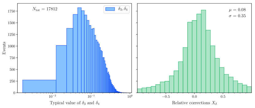
In the left pane in Fig. 3, we show typical values of $\delta_{3}$ and $\delta_{4}$ for selected events. The distribution peaks at $\delta_{3}\sim\delta_{4}\sim\sqrt{\lambda}\sim 0.1$ which is sufficiently small to justify the expansion in powers of $\sqrt{\lambda}$. In the right pane in Fig. 3, we show the distribution of $X_{\delta}$ defined in Eq. (72) for selected events. We see that, on average, the next-to-eikonal corrections reproduce the evaluation of the exact one-loop amplitude subject to WBF cuts. The $X_{\delta}$-distribution peaks at around $0.1$ which confirms our expectation that $X_{\delta}\sim\sqrt{\lambda}$. However, the distribution is fairly broad, which means that neglected terms amount to about $30\%$ of the next-to-eikonal contribution. This is consistent with magnitude of terms that we neglected by truncating the $\lambda$-expansion at ${\cal O}(\sqrt{\lambda})$ accuracy.

Figure 4: Eikonal and next-to-eikonal contributions to the transverse momentum and rapidity distributions of the leading jet. In the upper pane, leading eikonal contribution is plotted with a red, dashed line and the next-to-eikonal one with a green, solid line. In the lower pane, we show the ratio of next-to-eikonal to eikonal contributions. We note that in the upper left pane, absolute values are shown. See text for further details.

We are now in position to investigate the impact of next-to-eikonal corrections on the WBF cross section. The cross section reads

$$\,d\sigma=\sum_{i,j}\int\,dx_{1}\,dx_{2}\,f_{i}(x_{1},\mu_{F})\,d\hat{\sigma}_{nf}^{\textrm{NNLO}}(x_{1},x_{2},\mu_{R})\,f_{j}(x_{2},\mu_{F})\,,$$ (74)

where $f_{i,j}$ are parton distribution functions and $d\hat{\sigma}_{nf}^{\textrm{NNLO}}(x_{1},x_{2},\mu_{R})$ is the partonic WBF cross section that includes non-factorizable corrections computed through next-to-eikonal approximation. We employ NNPDF31_nnlo_as_0118 parton distribution functions Buckley:2014ana and use dynamical renormalization and factorization scales

$$\mu_{F}=\mu_{R}=\frac{m_{H}}{2}\left[1+\frac{4p_{H,\perp}^{2}}{m_{H}^{2}}\right]^{1/4}\,.$$ (75)

We set the mass of the $W$ boson to $m_{W}=80.398\textrm{ GeV}$, the mass of the $Z$ boson to $m_{Z}=91.1876\textrm{ GeV}$, and the mass of the Higgs boson to $m_{H}=125\textrm{ GeV}$. The Fermi constant is taken to be $G_{F}=1.16637\times 10^{-5}\textrm{ GeV}^{-2}$.

For $13\textrm{ TeV}$ proton-proton collisions, we find that the non-factorizable, double-virtual contribution to Higgs boson production in WBF evaluates to

$$\sigma_{VV}=\left(-3.1+0.53\right)\textrm{ fb}\,,$$ (76)

where we display contributions of leading and next-to-leading terms in the $\lambda$-expansion. We emphasise that the next-to-eikonal correction is calculated by excluding kinematic configurations where $|y_{H}|>1$ in the partonic center-of-mass frame, in addition to conventional WBF cuts that we listed earlier. It follows from Eq. (76) that the correction to the leading eikonal approximation amounts to $\mathcal{O}(17\%)$.

Figure 5: Eikonal and next-to-eikonal contributions to the transverse momentum and rapidity distributions of the Higgs boson. In the upper pane, leading eikonal contribution is plotted with a red, dashed line and the next-to-eikonal one with a green, solid line. In the lower pane, we show the ratio of next-to-eikonal to eikonal contributions.

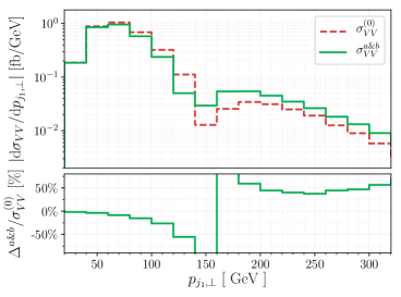
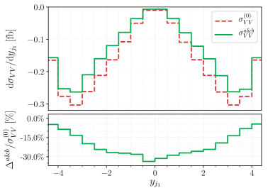
We now turn to the discussion of kinematic distributions. In Fig. 4, we display non-factorizable corrections to transverse momentum and rapidity distributions of the leading jet. The comparison of leading and next-to-leading eikonal contributions in lower panes shows that next-to-leading eikonal corrections range from ten to fifty percent. They appear to modify the leading order eikonal contribution by ${\cal O}(50\%)$ for higher values of $p_{\perp,j_{1}}$. This enhancement is partially related to the fact that the leading eikonal contribution changes sign at around $p_{\perp,j_{1}}\sim 2m_{W}$, which is the reason for rapidly changing ratio of eikonal factors shown in the lower pane.

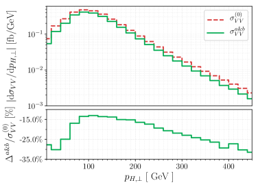
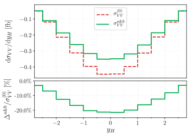
The non-factorizable contributions to Higgs boson transverse momentum and rapidity distributions are shown in Fig. 5. The relation between eikonal and next-to-eikonal contributions are similar to what was observed for the fiducial cross section as well as $p_{\perp}$ and rapidity distributions of the leading jet.

7 Conclusion

We computed the two-loop virtual non-factorizable QCD corrections to Higgs boson production in weak boson fusion through next-to-leading order in the eikonal expansion. We found that such an expansion proceeds in powers of $p_{\perp,H}/\sqrt{s}\sim m_{H}/\sqrt{s}$ and explained how to simplify the integrand of the two-loop amplitude to calculate both the leading and the next-to-leading terms in such an expansion.

We observed that combining individual diagrams before integrating over loop momenta leads to significant simplifications in the calculation. This happens because contributions of some of the virtual-momenta regions, that are relevant for computing next-to-eikonal corrections in individual Feynman diagrams, receive additional suppression in the full amplitude and start contributing only at next-to-next-to-leading power.

We have derived compact integral representations for the double-virtual non-factorizable amplitude at both leading and next-to-leading power in the eikonal expansion. We have also explained how to compute the two-loop amplitude analytically and provided the analytic results in the ancillary file.

The numerical impact of next-to-eikonal corrections is significant although, given the overal smallness of non-factorizable contributions, they do not change the original conclusions of Refs. Liu:2019tuy ; Dreyer:2020urf . Nevertheless, we find that, typically, the next-to-eikonal corrections change the estimate of the non-factorizable contributions based on the leading term in the eikonal expansion by ${\cal O}(20)$ percent.

As a final comment, we note that other sources of non-factorizable contributions to WBF cross sections, including double-real emission and the real-virtual corrections, were recently studied in Ref. Asteriadis:2023nyl . It was found that, thanks to the WBF cuts, all the contributions beyond the double-virtual ones are tiny and cannot impact the phenomenological studies of Higgs production in WBF in any way. The results reported in this reference allow us to estimate the contribution of the non-factorizable double-virtual corrections to the WBF cross section with a precision that is likely better than ${\cal O}(10)$ percent. Since the non-factorizable contribution itself is just ${\cal O}(1)$ percent of the total WBF cross section, the remaining uncertainties stemming from the imprecise knowledge of the two-loop virtual amplitude are irrelevant. We conclude that the current understanding of non-factorizable effects is sufficient for phenomenological studies of Higgs production in weak boson fusion envisaged for the Run III and the high-luminosity phase of the LHC.

8 Acknowledgments

We would like to thank A. Penin for useful conversations about non-factorizable effects in Higgs production in WBF. We are grateful to K. Asteriadis and Ch. Brønnum-Hansen for their help with the implementation of next-to-eikonal corrections into a numerical code for computing non-factorizable contributions to the WBF cross section. This research is partially supported by the Deutsche Forschungsgemeinschaft (DFG, German Research Foundation) under the grant 396021762 - TRR 257. The diagrams in Figs. 1 and 2 were generated using Jaxodraw Binosi:2003yf .

Appendix A Calculation of two-dimensional master integrals

The goal of this appendix is to explain how the $d=2$ Feynman integrals that contribute to the coefficients $\mathcal{C}_{1,2}$ can be computed. We begin with the discussion of the two-loop case. Two-loop $d=2$ integrals that are required for computing $\mathcal{C}_{2}$ belong to the following integral family

$$j[a_{1},a_{2},a_{3},a_{4}]=\frac{(m_{V}^{2})^{2\epsilon}}{\pi^{d-2}\Gamma(1+\epsilon)^{2}}\int\frac{{\rm d}{\bf k}_{1,\perp}^{d-2}{\rm d}{\bf k}_{2,\perp}^{d-2}}{\Delta_{1}^{a_{1}}\Delta_{2}^{a_{2}}\Delta_{3,12}^{a_{3}}\Delta_{4,12}^{a_{4}}}.$$ (77)

These integrals depend on the transverse momenta of the outgoing jets and of the Higgs boson, as well as on the mass of the vector boson $V$. For later convenience, we introduce three dimensionless variables as

$$x=\frac{{\bf p}_{3,\perp}^{2}}{m_{V}^{2}},\quad y=\frac{{\bf p}_{4,\perp}^{2}}{m_{V}^{2}},\quad z=\frac{{\bf p}_{H,\perp}^{2}}{m_{V}^{2}}.\quad$$ (78)

It is straighforward to write down integration-by-parts (IBP) identities Tkachov:1981wb ; Chetyrkin:1981qh for the integral family $j[a_{1},a_{2},a_{4},a_{4}]$. Performing the IBP reduction with LiteRed Lee:2012cn ; Lee:2013mka , we find that there are six master integrals. They are

$$f_{1} =j[2,1,2,0], f_{2} =j[2,2,1,0], f_{3} =j[2,1,0,2],$$ (79)

$$f_{4} =j[2,2,0,1], f_{5} =j[2,1,1,1], f_{6} =j[2,1,2,1].$$

$f_{1}$

$f_{2}$

$f_{3}$

$f_{4}$

$f_{5}$

$f_{6}$

Figure 6: Two-dimensional two-loop master integrals. The thick and thin internal lines represent massive and massless propagators, respectively. Red lines have mass $m_{V}$. The black thick lines correspond to external ”massive” legs. A dot on the internal line means raising the power of corresponding propagator by one.

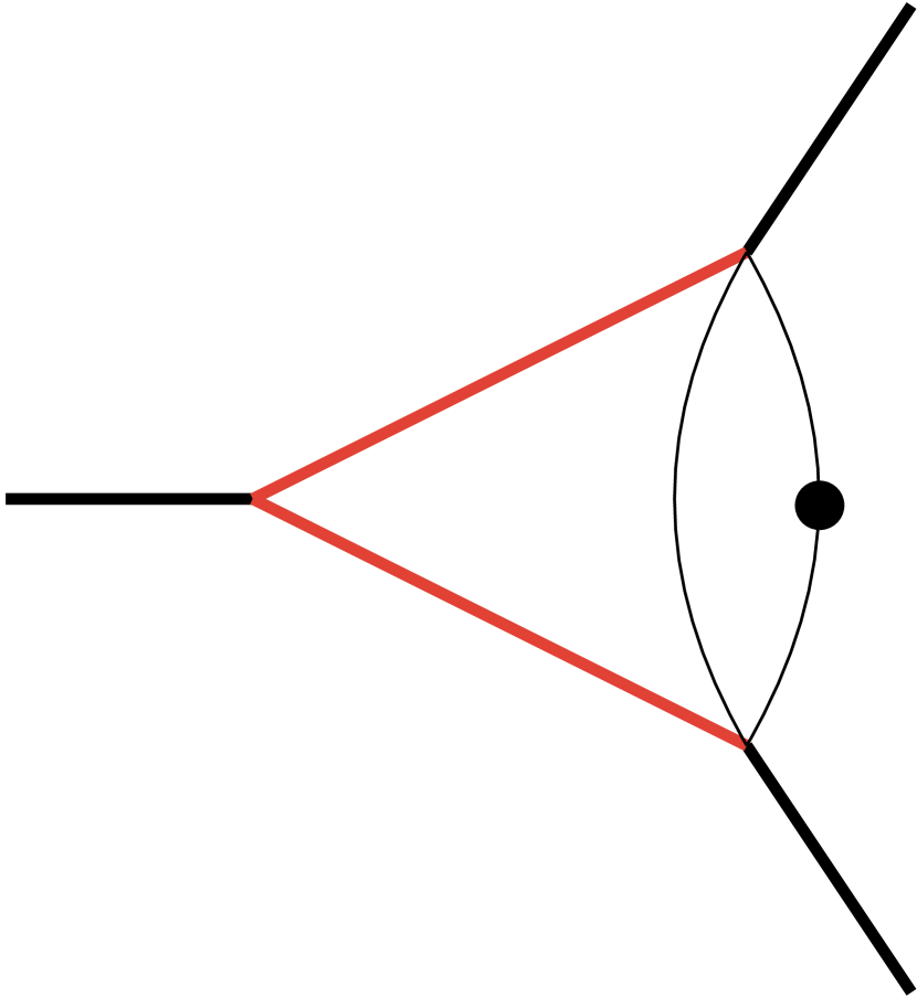
The master integrals are displayed in Fig. 6. Although we need these integrals at $d=2$, we find it more convenient to study them first in four dimensions. In particular, at $d=4$, we easily obtain the canonical basis Henn:2013pwa using the Magnus series expansion method Argeri:2014qva . We then transform the integrals to $d=2$ using the dimensional recurrence relations Tarasov:1996br . In four dimensions, the canonical basis reads

$$g_{1} =x\epsilon^{2}m_{V}^{2}f_{1},$$

$$g_{2} =2\epsilon^{2}m_{V}^{2}f_{1}+(x+1)\epsilon^{2}m_{V}^{2}f_{2},$$

$$g_{3} =y\epsilon^{2}m_{V}^{2}f_{3},$$

$$g_{4} =2\epsilon^{2}m_{V}^{2}f_{3}+(y+1)\epsilon^{2}m_{V}^{2}f_{4},$$

$$g_{5} =2\epsilon^{3}m_{V}^{2}r_{2}f_{5},$$ (80)

$$g_{6} =\frac{\epsilon^{2}r_{1}m_{V}^{2}}{4[2(y-x)+z(1+y)]}\Bigg{\{}4m_{V}^{2}[(x-y)^{2}-(x+1)(y+1)z]f_{6}$$

$$\qquad-6\epsilon[(x-y)(y-1)+z(1+y)]f_{5}+(y+1)^{2}(f_{4}+2f_{3})$$

$$\qquad-(x+1)(y+1)(f_{2}+2f_{1})\Bigg{\}},$$

where $r_{1,2}$ represent two square roots,

$$r_{1}=\sqrt{z(z+4)},\qquad r_{2}=\sqrt{(x+y-z)^{2}-4xy}.$$ (81)

Note that all the $g$’s are normalized to be dimensionless and can be regarded as functions of $x,y$ and $z$ only. The canonical basis vector $\vec{g}=(g_{1},g_{2},g_{3},g_{4},g_{5},g_{6})^{T}$ satisfies a differential equation in the $d{\rm log}$ form,

$$d\vec{g}(x,y,z;\epsilon)=\epsilon(d\mathbb{A})\;\vec{g}(x,y,z;\epsilon),$$ (82)

where the matrix $\mathbb{A}$ reads

and the 14 logarithms that constitute $\mathbb{A}$ are

$$l_{1} =\log(x), l_{2} =\log(x+1), l_{3} =\log(y),$$

$$l_{4} =\log(y+1), l_{5} =\log(z), l_{6} =\log(z+4),$$

$$l_{7} =\hbox to0.0pt{$\displaystyle\log\left[(x-y)^{2}-(x+1)(y+1)z\right],\,l_{8}=\log\left(\frac{z+2-r_{1}}{z+2+r_{1}}\right),\,l_{9}=\log\left(r_{2}\right),$\hss}$$

$$l_{10} =\log\left(\frac{x-y+z-r_{2}}{x-y+z+r_{2}}\right), l_{11} =\log\left(\frac{-x+y+z-r_{2}}{-x+y+z+r_{2}}\right),$$ (84)

$$l_{12} =\log\left(\frac{r_{1}-r_{2}+x-y}{r_{1}+r_{2}+x-y}\right), l_{13} =\log\left(\frac{r_{1}-r_{2}+x-y}{r_{1}+r_{2}-x+y}\right),$$

$$l_{14} =\log\left(\frac{r_{1}-r_{2}-x+y}{r_{1}+r_{2}-x+y}\right).$$

Eq. (82) can be recursively solved order-by-order in $\epsilon$ and the solutions are expressed in terms of Chen’s iterated integrals Chen:1977oja with some boundary constants that cannot be determined from the differential equations alone. For the integrals $g_{1,..,6}$ these constants can be computed with a relative ease since all canonical integrals, except $g_{2}$ and $g_{4}$, vanish when $x=y=z=0$. The non-vanishing integrals $g_{2}$ and $g_{4}$ at this kinematic point evaluate to

$$g_{2,4}(0,0,0)=-\frac{\pi\epsilon\csc(\pi\epsilon)\Gamma(1+2\epsilon)}{\Gamma(1+\epsilon)^{2}}=-1-\frac{\pi^{2}}{3}\epsilon^{2}+\mathcal{O}\left(\epsilon^{3}\right).$$ (85)

Furthermore, under the change of variables

$$x=zuv,\quad y=z(1-u)(1-v),\quad z=\frac{(1-w)^{2}}{w},$$ (86)

the square roots $r_{1,2}$ are rationalized simultaneously and we find

$$r_{1}=\frac{(1-w)(1+w)}{w},\qquad r_{2}=\frac{(1-w)^{2}(u-v)}{w}.$$ (87)

As the result, the solutions of the system Eq. (82) can be expressed in terms of multiple polylogarithms. In fact, since we need $\vec{g}$ only through ${\cal O}(\epsilon^{2})$, relevant expressions for integrals involve logarithms and dilogarithms of $u,v,w$. To express them in terms of $x,y,z$, we use the following formulas

$$u,v=\frac{x-y+z\pm r_{2}}{2z},\quad w=\frac{2+z-r_{1}}{2}.$$ (88)

Finally, to compute the one-loop amplitude, we need to study the following integral family

$$j[a_{1},a_{2},a_{3}]=\frac{(m_{V}^{2})^{\epsilon}}{\pi^{(d-2)/2}\Gamma(1+\epsilon)}\int\frac{{\rm d}{\bf k}_{1,\perp}^{d-2}}{\Delta_{1}^{a_{1}}\Delta_{3,1}^{a_{2}}\Delta_{4,1}^{a_{3}}}.$$ (89)

The analysis is identical to the two-loop case and we will not repeat it here. We only mention that the canonical basis at $d=2$ reads

$$g_{1} =\epsilon j[0,0,1],$$

$$g_{2} =\epsilon j[0,1,1]m_{V}^{2}r_{1},$$

$$g_{3} =\epsilon j[1,0,1]m_{V}^{2}\left(1+y\right),$$

$$g_{4} =\epsilon j[1,1,0]m_{V}^{2}\left(1+x\right),$$

$$g_{5} =\frac{\epsilon m_{V}^{2}}{2r_{2}}\Big{\{}2j[1,1,1]m_{V}^{2}\left[(x-y)^{2}-(1+x)(1+y)z\right]$$ (90)

$$\qquad+j[1,1,0]\left[\left(-x+y-z\right)+x\left(x-y-z\right)\right]$$

$$\qquad-j[1,0,1]\left[\left(-x+y+z\right)+y\left(x-y+z\right)\right]$$

$$\qquad+j[0,1,1]\left(2-x-y+z\right)z\Big{\}}.$$

The canonical basis statisfies a differential equation in the $d{\rm log}$ form, similar to Eq. (82). The corresponding matrix $\mathbb{A}$ reads

where the logarithms, $l_{i}$, are given in Eq. (A). To compute the boundary constants, we use the fact that the basis is finite at $x=y=z=0$ and $g_{1}=-1$.

References

- (1) T. Liu, K. Melnikov and A.A. Penin, Nonfactorizable QCD Effects in Higgs Boson Production via Vector Boson Fusion, Phys. Rev. Lett. 123 (2019) 122002 [1906.10899].
- (2) CMS collaboration, Search for the standard model Higgs boson produced through vector boson fusion and decaying to , Phys. Rev. D 92 (2015) 032008 [1506.01010].
- (3) CMS collaboration, Combined measurements of Higgs boson couplings in proton–proton collisions at , Eur. Phys. J. C 79 (2019) 421 [1809.10733].
- (4) ATLAS collaboration, Search for Higgs bosons produced via vector-boson fusion and decaying into bottom quark pairs in collisions with the ATLAS detector, Phys. Rev. D 98 (2018) 052003 [1807.08639].
- (5) ATLAS collaboration, Combined measurements of Higgs boson production and decay using up to fb-1 of proton-proton collision data at 13 TeV collected with the ATLAS experiment, Phys. Rev. D 101 (2020) 012002 [1909.02845].
- (6) T. Figy, C. Oleari and D. Zeppenfeld, Next-to-leading order jet distributions for Higgs boson production via weak boson fusion, Phys. Rev. D 68 (2003) 073005 [hep-ph/0306109].
- (7) E.L. Berger and J.M. Campbell, Higgs boson production in weak boson fusion at next-to-leading order, Phys. Rev. D 70 (2004) 073011 [hep-ph/0403194].
- (8) P. Bolzoni, F. Maltoni, S.-O. Moch and M. Zaro, Higgs production via vector-boson fusion at NNLO in QCD, Phys. Rev. Lett. 105 (2010) 011801.
- (9) P. Bolzoni, F. Maltoni, S.-O. Moch and M. Zaro, Vector boson fusion at NNLO in QCD: SM Higgs and beyond, Phys. Rev. D 85 (2012) 035002.
- (10) M. Cacciari, F.A. Dreyer, A. Karlberg, G.P. Salam and G. Zanderighi, Fully Differential Vector-Boson-Fusion Higgs Production at Next-to-Next-to-Leading Order, Phys. Rev. Lett. 115 (2015) 082002 [1506.02660].
- (11) J. Cruz-Martinez, T. Gehrmann, E.W.N. Glover and A. Huss, Second-order QCD effects in Higgs boson production through vector boson fusion, Phys. Lett. B 781 (2018) 672 [1802.02445].
- (12) M. Ciccolini, A. Denner and S. Dittmaier, Electroweak and QCD corrections to Higgs production via vector-boson fusion at the LHC, Phys. Rev. D 77 (2008) 013002 [0710.4749].
- (13) F.A. Dreyer and A. Karlberg, Vector-Boson Fusion Higgs Production at Three Loops in QCD, Phys. Rev. Lett. 117 (2016) 072001 [1606.00840].
- (14) M. Beneke and V.A. Smirnov, Asymptotic expansion of Feynman integrals near threshold, Nucl. Phys. B 522 (1998) 321 [hep-ph/9711391].
- (15) B. Jantzen, Foundation and generalization of the expansion by regions, JHEP 12 (2011) 076 [1111.2589].
- (16) B. Jantzen, A.V. Smirnov and V.A. Smirnov, Expansion by regions: revealing potential and Glauber regions automatically, Eur. Phys. J. C 72 (2012) 2139 [1206.0546].
- (17) S. Catani, The Singular behavior of QCD amplitudes at two loop order, Phys. Lett. B 427 (1998) 161 [hep-ph/9802439].
- (18) L. Gates, On Evaluation of Nonfactorizable Corrections to Higgs Boson Production via Vector Boson Fusion, 2305.04407.
- (19) K. Asteriadis, F. Caola, K. Melnikov and R. Röntsch, NNLO QCD corrections to weak boson fusion Higgs boson production in the H → b and H → WW∗ → 4l decay channels, JHEP 02 (2022) 046 [2110.02818].
- (20) A. Buckley, J. Ferrando, S. Lloyd, K. Nordström, B. Page, M. Rüfenacht et al., LHAPDF6: parton density access in the LHC precision era, Eur. Phys. J. C 75 (2015) 132 [1412.7420].
- (21) F.A. Dreyer, A. Karlberg and L. Tancredi, On the impact of non-factorisable corrections in VBF single and double Higgs production, JHEP 10 (2020) 131 [2005.11334].
- (22) K. Asteriadis, C. Brønnum-Hansen and K. Melnikov, On the non-factorizable corrections to Higgs boson production in weak boson fusion, 2305.08016.
- (23) D. Binosi and L. Theussl, JaxoDraw: A Graphical user interface for drawing Feynman diagrams, Comput. Phys. Commun. 161 (2004) 76 [hep-ph/0309015].
- (24) F.V. Tkachov, A Theorem on Analytical Calculability of Four Loop Renormalization Group Functions, Phys. Lett. B 100 (1981) 65.
- (25) K.G. Chetyrkin and F.V. Tkachov, Integration by Parts: The Algorithm to Calculate beta Functions in 4 Loops, Nucl. Phys. B 192 (1981) 159.
- (26) R.N. Lee, Presenting LiteRed: a tool for the Loop InTEgrals REDuction, 1212.2685.
- (27) R.N. Lee, LiteRed 1.4: a powerful tool for reduction of multiloop integrals, J. Phys. Conf. Ser. 523 (2014) 012059 [1310.1145].
- (28) J.M. Henn, Multiloop integrals in dimensional regularization made simple, Phys. Rev. Lett. 110 (2013) 251601 [1304.1806].
- (29) M. Argeri, S. Di Vita, P. Mastrolia, E. Mirabella, J. Schlenk, U. Schubert et al., Magnus and Dyson Series for Master Integrals, JHEP 03 (2014) 082 [1401.2979].
- (30) O.V. Tarasov, Connection between Feynman integrals having different values of the space-time dimension, Phys. Rev. D 54 (1996) 6479 [hep-th/9606018].
- (31) K.-T. Chen, Iterated path integrals, Bull. Am. Math. Soc. 83 (1977) 831.