Robust data-driven Lyapunov analysis with fixed data

Abstract

In this era of digitalization, data has widely been used in control engineering. While stability analysis is a mainstay for control science, most stability analysis tools still require explicit knowledge of the model or a high-fidelity simulator. In this work, a new data-driven Lyapunov analysis framework is proposed. Without using the model or its simulator, the proposed approach can learn a piece-wise affine Lyapunov function with a finite and fixed off-line dataset. The learnt Lyapunov function is robust to any dynamics that are consistent with the off-line dataset. Along the development of proposed scheme, the Lyapunov stability criterion is generalized. This generalization enables an iterative algorithm to augment the region of attraction.

Keywords

Data-driven method, Lyapunov stability analysis

Acknowledgments

This work was supported by the Swiss National Science Foundation under the “NCCR Automation” grant number 51NF40_180545.

The work of M. Tacchi was also supported by the French company RTE, under the RTE-EPFL partnership n^∘2022–0225.

1 Introduction

Stability analysis is a major research topic in control science. Among various stability criteria, Lyapunov analysis [1] plays a key role in this field. In this framework, stability analysis is reformulated into the search for a Lyapunov function. This has been widely studied in the model-based or sampling-based setup, where the user is assumed to have direct access to the model or its high-fidelity simulator. Note that the system model or its simulator may not be available all the time, it is usually possible and much easier to measure a finite number of system responses offline. Therefore, stability analysis based on fixed measured data poses a new challenge and becomes desirable. Motivated by this need, this work studies the Lyapunov analysis based on a given finite set of measurements of system response. The proposed approach can learn a piece-wise affine (PWA) Lyapunov function on a compact set without access to the system model/simulator. The contributions of this work are summarized as follows:

• We formulate and prove a Lyapunov inference theorem, which generalizes existing Lyapunov stability analysis methods. This generalization is used to expand a prior inner estimate of the region of attraction to a larger set.

• We specify our Lyapunov stability criterion for PWA Lyapunov function on a compact set, to make it verifiable locally on this compact set rather than at all points.

• We make the Lyapunov criterion robust to all the models that are consistent with the measured dataset. This criterion is defined on general bounded evaluation function spaces, and has a convex form for Lipschitz functions.

• We develop an algorithm to learn a Lyapunov function robust to all models that are consistent with the measured dataset. The proposed algorithm only needs to solve a convex second-order cone program, regardless of the underlying unknown dynamics (non-)linearity.

• We discuss numerical results properties of the proposed algorithm, mostly focusing on the improvement of its computational efficiency.

Previous Work

Nonlinear Lyapunov stability analysis has been widely studied, where model-based approaches and sampling-based approaches form two main categories. In either approach, a Lyapunov candidate is optimized or synthesized by verifying the Lyapunov stability conditions. In the model-based approaches, the knowledge of the underlying model is explicitly used in the search of the Lyapunov function. On the contrary, the Lyapunov function is trained by penalizing the violation of the Lyapunov stability conditions on a dataset. Even though a standard Monte-Carlo sampling scheme can also give a probabilistic guarantee [2], it is always preferable to give a strict qualification in stability analysis. In this case, both model-based approaches and sample-based approaches require the explicit knowledge of the model. In particular, verification of the Lyapunov stability condition usually resort to nonlinear optimization or satisfiability modulo theory (SMT) solvers, such as dReal [3]. Note that when smooth dynamics are considered, one can write the Lyapunov stability condition with respect to any Lyapunov candidate into an explicit algebraic form (see e.g [4, 5, 6]). The SMT solver is accordingly used to check whether these algebraic inequalities are satisfied up to some user-defined tolerance [7].

To the best of the authors’ knowledge, the first numerical method that finds a Lyapunov function solves the Zubov equation [8]. The Zubov equation models the Lyapunov function as the solution to a linear partial differential equation (PDE). The approximation of this PDE is solved by series expansion [8], collocation method [9], etc. One main advantage of the model-based approach is that the a-priori knowledge about the model can be used to reformulate the Lyapunov learning problem into a simpler problem. When polynomial dynamics are considered, a sum of square (SOS) programming relaxation can be used to search for polynomial Lyapunov functions [10]. Due to the nice algebraic properties of polynomials, the SOS framework has been further used to find the region of attraction [11, 12] and its sparsity structure has been used to improve its scalability [13, 14]. Parallel to the studies in polynomial dynamics, PWA dynamics is another genre attracting broad research interest [15, 16]. Such tremendous interest is also a result of the ubiquitous appearances of PWA functions in various controllers, such as ReLU-neural-networks-based controller and linear MPC [17]. For the PWA setup, optimization based approaches play the central role, which mostly applies linear matrix inequality  [18, 12, 19] and mixed integer programming [20].

Unlike the model-based approaches, sampling-based methods highly rely on an efficient strategy of generating informative samples. The counter-example guided inductive synthesis (CEGIS) [21, 22] is one major concept applied behind many sample-based approaches (see e.g. [23, 19, 24]). These approaches have direct access to the model or its simulator. During the learning process, they iteratively augment the sample dataset by adding counter examples to the Lyapunov candidate proposed in the current iteration. These algorithms train the Lyapunov function by penalizing the violation of the Lyapunov stability condition on the samples, and they converge when no further counter example can be generated [23, 5].

The search for a Lyapunov function is usually confined to a specific function class, such as generalized quadratic form [25] or positive definite kernel regressor [26]. In this work, we will focus on PWA Lyapunov functions defined on a compact set. Besides the advantages mentioned in the model-based approach paragraph, PWA Lyapunov candidates have shown nice interplay with Lipschitz dynamics. In particular, when the samples of system dynamics are assigned to the vertices of a grid, a robust Lyapunov stability condition on each simplex can be verified by only considering a tightened Lyapunov condition defined on its vertices. This family of methods is called the continuous piece-wise affine (CPA) method [27, 28]. The CPA method has been extended to more general problem setup: differential inclusion [29], switched system [30], etc. In this work, we also consider Lipschitz dynamics, but we do not assume that the data are located on the vertices. Therefore, we do not term our method a CPA method to avoid unnecessary confusion. More detailed comparison with the CPA method are postponed to Section 4.3.

The rest of this paper is organized as follows: In Section 2, some necessary tools from convex analysis are reviewed alongside the statement of the problem setup. In Section 3, we will first generalize the Lyapunov theorem in Section 3.1, this generalization will later be used to develop a local Lyapunov condition with PWA Lyapunov candidate in Section 3.2. In the sequel, Section 4 applies this local condition to a set of uncertain function defined by data, whose robust satisfaction is summarized as in Theorem 4. This theorem is later used to define a convex inequality condition for the class of Lipschitz function in Section 4.2, where the learning problem will be summarized. A comparison between the proposed learning problem and other related works are given in Section 4.3. The learnability of the proposed scheme is studied in Section 5.1, after which the proposed learning problem is recast into an equivalent form to enable higher computational efficiency in Section 5.2. The general learning algorithm are summarized in 5.3 with a numerical validation in Section 6. A conclusion wraps up this paper in Section 7.

Notation: $\{x_{i}\}_{i\in\mathcal{I}}$ is a set indexed by $\mathcal{I}$, and when there is no confusion, we drop the index set with $\{x_{i}\}$. $\mathbb{N}_{a}$ denotes the set of positive integer less than $a$. $\mathbb{R}_{+}$ denotes the set of non-negative real numbers. 0 is a zero vector. $\mathcal{B}(x,r)$ denotes an open euclidean ball centred at $x$ with radius $r$. $\mathrm{co}(\mathcal{X})$ denotes the convex hull of $\mathcal{X}\subset\mathbb{R}^{n}$. $\mathrm{Lip}(\mathcal{X})$ is the set of Lipschitz functions defined on $\mathcal{X}$.

If $A:\mathcal{H}_{x}\longrightarrow\mathcal{H}_{y}$ is a linear operator mapping between Hilbert spaces $\mathcal{H}_{x}$ and $\mathcal{H}_{y}$, then $A^{*}$ denotes its adjoint as $A^{*}:\mathcal{H}_{y}\longrightarrow\mathcal{H}_{x}$. $X\setminus Y:=\{x\in X\;|\;x\notin Y\}$ for all $Y\subset X$. $\lVert x\rVert$ denotes the norm of $x\in\mathbb{R}^{n}$, whose dual norm is denoted by $\lVert x\rVert^{*}$, if not specified, $\lVert\cdot\rVert$ denotes the euclidean norm (in which case $\lVert\cdot\rVert^{*}=\lVert\cdot\rVert$). $|C|$ denotes the cardinality of a set $C$. If $\mathcal{X}$ is a topological space, then $\mathrm{int}(\mathcal{X})$, $\overline{\mathcal{X}}$ and $\partial\mathcal{X}$ denote its interior, closure and boundary, respectively.

Finally, due to ambiguity in the literature, we indicate our definition of polyhedra and polytopes:

• A polyhedron $P\subset\mathbb{R}^{n}$ is an intersection of finitely many half spaces: $\exists m\;\in\mathbb{N},A\in\mathbb{R}^{m\times n},b\in\mathbb{R}^{m}$ such that

  $$P=\{x\in\mathbb{R}^{n}\;|\;Ax-b\in(\mathbb{R}_{+})^{m}\}\;.$$

  When the polyhedron is bounded, with slightly abuse of notation, we denote the number of vertices by $|P|$.

• A polytope is a finite union of bounded polyhedra, which is not necessarily convex. Accordingly, a convex polytope is the convex hull of its vertices.

2 Preliminary

In this section, we will first review some results from convex analysis and then introduce the considered stability analysis problem.

2.1 Convex Analysis

Let $\mathbb{R}_{C}^{n}$ denote the set of compact convex subsets in $\mathbb{R}^{n}$, the support function of a compact set $C\in\mathbb{R}_{C}^{n}$ is defined by

$$V_{C}(g):=\max\limits_{x\in C}g^{\top}x\;,$$

for all $g\in\mathbb{R}^{n}$, and any convex set can be uniquely characterized by its support function. Meanwhile, the indicator function of a convex set $C\in\mathbb{R}_{C}^{n}$ is defined by

$$\iota_{C}(x):=\begin{cases}0\;,&x\in C\\ \infty\;,&x\notin C\;,\end{cases}$$

and this function is convex. With this definition, we also have

$$\iota_{C_{1}\cap C_{2}}(x)=\iota_{C_{1}}(x)+\iota_{C_{2}}(x)\;,$$ (1)

as $\iota_{C_{1}\cap C_{2}}(x)=0$ if and only if $\iota_{C_{1}}(x)=0$ (i.e. $x\in C_{1}$) and $\iota_{C_{2}}(x)=0$ (i.e. $x\in C_{2}$), and thus $x\in C_{1}\cap C_{2}$. A conjugate of a convex function $h:\mathbb{R}^{n}\rightarrow\mathbb{R}$ is defined, for $g\in\mathbb{R}^{n}$, by

$$h^{*}(g):=\max\limits_{x\in\mathbb{R}^{n}}g^{\top}x-h(x)\;.$$

By this definition, the conjugate of a non-empty set indicator function is its support function [31, 11.4] as

$$V_{C}(\cdot)=\iota^{*}_{C}(\cdot)\;.$$

Given two proper, convex functions $h_{1}:\mathbb{R}^{n}\longrightarrow\mathbb{R}$ and $h_{2}:\mathbb{R}^{n}\longrightarrow\mathbb{R}$, the infimal convolution is defined by

$$h_{1}\#h_{2}(x) :=\inf_{y\in\mathbb{R}^{n}}h_{1}(y)+h_{2}(x-y)\;,$$

Geometrically, the epigraph of $h_{1}\#h_{2}(\cdot)$ is the Minkowski sum of the epigraph of $h_{1}(\cdot)$ and $h_{2}(\cdot)$:

$$\left\{\vphantom{\sum}(x,s)\in\mathbb{R}^{n}\times\mathbb{R}\;:\;h_{1}\#h_{2}(x)<s\right\}=\left\{\vphantom{\sum}(y+z,p+q)\in\mathbb{R}^{n}\times\mathbb{R}\;:\;h_{1}(y)<p\ \wedge\ h_{2}(z)<q\right\}.$$

In particular, $h_{1}(\cdot)$ and $h_{2}(\cdot)$ being proper and convex, so is $h_{1}\#h_{2}$. For the sake of simplicity, we denote

$$\#_{i}h_{i}(x) :=\inf\sum_{i}h_{i}(y_{i})\;\;\;\text{s.t. }\sum_{i}y_{i}=x\;.$$

By Lagrangian multiplier, the following calculus of infimal convolution can be derived [32]

Proposition 1.

Let $h_{1},\;h_{2}$ be two proper, convex functions, then

$$\left(h_{1}+h_{2}\right)^{*}(x)=h_{1}^{*}\#h_{2}^{*}(x)\;,$$

2.2 Unknown dynamic system, fixed data

In our problem setup, we consider an unknown continuous time dynamic system on a dimension $n_{x}$ compact set $\mathcal{X}\subset\mathbb{R}^{n_{x}}$,

$$\frac{dx}{dt}=f(x)\;,$$

which we know has a locally asymptotically stable (LAS) equilibrium point (EP). And we have a size $N_{D}$ fixed dataset sampled from this system as $D=\{(x_{i},f_{i}=f(x_{i}))\}_{i=1}^{N_{D}}$ with $x_{i}\in\mathcal{X}$. The goal is to analyse the stability of this unknown dynamical system based on the fixed dataset $D$. Without loss of generality, we assume that

Assumption 1.

$\mathbf{0}\in\mathcal{X}$ is the LAS EP and we have access to a compact subset $\mathcal{X}_{s}$ of its region of attraction.

Note that $\mathcal{X}_{s}$ models a conservative prior about the region of attraction (RoA) of the unknown dynamic system, e.g. deduced from engineering practice. Meanwhile, if no such information is available, one can also consider $\mathcal{X}_{s}=\{\mathbf{0}\}$. We denote the vector space of Lipschitz continuous functions on $n_{x}$ dimensional domain $\mathcal{X}$ by $\mathrm{Lip}(\mathcal{X})^{n_{x}}$ . To facilitate the analysis, we further assume that

Assumption 2.

$f\in\mathcal{F}$ where $\mathcal{F}\subset\mathrm{Lip}(\mathcal{X})^{n_{x}}$ is a vector space of Lipschitz continuous functions, such that

$$\forall\;h\in\mathcal{F},x\mapsto\|h(x)\|\text{ is bounded within }\mathcal{X},$$

with upper bound denoted $\|h\|_{\infty}$ (clearly a norm on $\mathcal{F}$).

Remark 1.

Assumption 2 means that the underlying dynamic system is bounded within $\mathcal{X}$ (i.e. there will not exist infinite velocity). Meanwhile, $\mathcal{F}$ does not need to be a Hilbert space, a typical case being the whole $\mathrm{Lip}(\mathcal{X})^{n_{x}}$. If a Hilbert space $\mathcal{F}$ is used, it is usually assumed to be infinite dimensional to ensure a large modelling capability.

Remark 2.

Assumption 2 implies that the evaluation operator defined by

$$E_{x}(h):=h(x)\;,\;\forall\;x\in\mathcal{X},\;h\in\mathcal{F}$$

is bounded (i.e. continuous in $h$) with respect to the norm $\|\cdot\|_{\infty}$, meaning that

$$\forall\;x\in\mathcal{X},\exists\;C_{x}\geq 0\;;\forall\;h\in\mathcal{F},\|E_{x}(h)\|\leq C_{x}\|h\|_{\infty}.$$

Indeed, taking $C_{x}=1$ for all $x\in\mathcal{X}$ is always possible. However, as soon as $\mathcal{F}$ contains the space of polynomial vector fields, it cannot be complete with respect to this norm $\|\cdot\|_{\infty}$, as the Stone-Weierstrass theorem ensures that its uniform completion is the whole space of continuous functions (including non-Lipschitz ones). As a result, one might prefer the standard Lipschitz norm

$$\|h\|_{\mathrm{Lip}}:=\|h(\mathbf{0})\|+\underset{\text{Lipschitz constant}}{\underbrace{\sup_{x\neq y\in\mathcal{X}}\frac{\|h(x)-h(y)\|}{\|x-y\|}}}$$

for which $\mathrm{Lip}(\mathcal{X})^{n_{x}}$ is complete and the $E_{x}$ are also bounded:

$$\|E_{x}(h)\| =\|h(x)\|$$

$$=\|h(\mathbf{0})+h(x)-h(\mathbf{0})\|$$

$$\leq\|h(\mathbf{0})\|+\|h(x)-h(\mathbf{0})\|$$

$$\leq\|h(\mathbf{0})\|+\|x\|\sup_{y\neq z\in\mathcal{X}}\frac{\|h(y)-h(z)\|}{\|y-z\|}$$

$$\leq\underset{C_{x}}{\underbrace{(1+\|x\|)}}\,\|h\|_{\mathrm{Lip}}$$

3 Piecewise affine functions for Lyapunov inference

In this section, we first try to augment the prior knowledge of stability in $\mathcal{X}_{s}$ to a bigger set $\mathcal{X}$ in Section 3.1. This result is refined to a Lyapunov candidate from the class of piece-wise affine (PWA) functions in in Section 3.2.

3.1 Lyapunov inference

Before proceeding to the stability condition, we introduce two additional concepts on functions $L:\mathbb{R}^{n_{x}}\rightarrow\mathbb{R}$. The sub-level set of $L$ with level $\alpha\in\mathbb{R}$ is given by

$$L_{\leq\alpha}:=\left\{x\in\mathbb{R}^{n_{x}}\;|\;L(x)\leq\alpha\right\}.$$

The Clarke generalized gradient of $L$ at a point $x\in\mathbb{R}^{n_{x}}$ is the set given by

$$\partial_{\mathrm{Cl}}L(x):=\mathrm{co}\left\{y\in\mathbb{R}^{n_{x}}:\begin{array}[]{l}\forall\;\epsilon>0,\exists\ x_{\epsilon}\in\mathbb{R}^{n_{x}};\\ \|x-x_{\epsilon}\|<\epsilon,\\ L\text{ is differentiable in }x_{\epsilon},\\ \|y-\nabla L(x_{\epsilon})\|<\epsilon\end{array}\right\}.$$

In [33, Theorem 2.5.1] it is proved that if $L$ is Lipschitz continuous on a neighbourhood of $x$, then $\partial_{\mathrm{Cl}}L(x)\neq\varnothing$. The Clarke gradient is a generalized gradient in the sense that if $L$ is continuously differentiable on a neighbourhood of $x$, then trivially $\partial_{\mathrm{Cl}}L(x)=\{\nabla L(x)\}$.

Now we summarize the Lyapunov stability condition on a compact set $\mathcal{X}$ in the following Lyapunov inference theorem.

Theorem 2.

Let Assumption 1 and 2 hold, and suppose that there exists a Lipschitz continuous function $L:\mathbb{R}^{n_{x}}\rightarrow\mathbb{R}$ such that:

1. There exists $\alpha\in\mathbb{R}$ such that $\mathcal{X}=L_{\leq\alpha}$.

2. $f(x)^{\top}y<0$ for all $x\in\mathcal{X}\setminus\mathcal{X}_{s}$, $y\in\partial_{\mathrm{Cl}}L(x)$.

Then for all $x_{0}\in\mathrm{int}(\mathcal{X})$,

$$x(t|x_{0})\underset{t\to\infty}{\longrightarrow}\mathbf{0}$$

where $t\mapsto x(t|x_{0})$ denotes the (unique by Lipschitz continuity of $f$ – see Assumption 2) continuously differentiable solution to the Cauchy problem

$$\begin{cases}\dfrac{d}{dt}x(t|x_{0})=f(x(t|x_{0}))\\ x(0|x_{0})=x_{0}.\end{cases}$$

Proof.

The proof is similar to the proof of the Lasalle theorem [34]. Let $x_{0}\in\mathrm{int}(\mathcal{X})$ and define the entering time

$$\tau(x_{0}):=\inf\{t\geq 0:x(t|x_{0})\in\mathcal{X}_{s}\}.$$

If $\tau(x_{0})<\infty$, then $x(\tau(x_{0})|x_{0})\in\mathcal{X}_{s}$ and using the semigroup property and Assumption 1, one obtains $x(t+\tau(x_{0})|x_{0})=x(t|x(\tau(x_{0}))\underset{t\to\infty}{\longrightarrow}\mathbf{0}$ so that $x(t|x_{0})\underset{t\to\infty}{\longrightarrow}\mathbf{0}$.

We now proceed to the non-trivial case where $\tau(x_{0})=\infty$, i.e. $\forall\;t\geq 0$, $x(t|x_{0})\notin\mathcal{X}_{s}$, and consider the exit time $T:=\inf\{t\geq 0:x(t|x_{0})\in\partial\mathcal{X}\}$. Notice that as $x_{0}\in\mathrm{int}(\mathcal{X})$ and $t\mapsto x(t|x_{0})$ is continuous, $T>0$. Then, using Lipschitz continuity of $L$, condition 2.2) and [35, Lemma 2.15], for almost all $t\in[0,T)$, $\frac{d}{dt}L(x(t|x_{0}))<0$, so that $L(x(t|x_{0}))$ is decreasing on $[0,T)$ by the mean value inequality. This yields that $\forall\;t\in(0,T)$, one has $L(x(t|x_{0}))<L(x_{0})\leq\alpha$, and by condition 2.1) and continuity of $t\mapsto L(x(t|x_{0}))$, $T=\infty$ and thus $L(x(t|x_{0}))$ is decreasing on $[0,\infty)$ and for all $t\geq 0$, $x(t|x_{0})\in\mathcal{X}\setminus\mathcal{X}_{s}$ regarding $\tau(x_{0})=\infty$.

We now consider the compact set $\Omega:=\overline{\mathcal{X}\setminus\mathcal{X}_{s}}$ from which the trajectory $x(t|x_{0})$ never escapes. Since $L$ is continuous and $\Omega$ is compact, by the Weierstrass extreme value theorem, one has that

$$-\infty<\ell:=\inf\limits_{\Omega}L,$$

so that the function $t\mapsto L(x(t|x_{0}))$ is decreasing and lower bounded, hence it has a limit $c:=\lim\limits_{t\to\infty}L(x(t|x_{0}))\in\mathbb{R}$ that it does not attain in finite time.

We also consider the limit set

$$\Gamma(x_{0}):=\{p\in\Omega:\forall\;\epsilon,T>0,\exists\;t\geq T;\|x(t|x_{0})-p\|<\epsilon\},$$

that has the following property (see [34]): as $t\mapsto x(t|x_{0})$ is bounded, $\Gamma(x_{0})\subset\Omega$ is nonempty, compact and invariant (forward and backwards). Thus, $\exists\;p_{0}\in\Gamma(x_{0})$ and $\forall\;t\geq 0$, $x(t|p_{0})\in\Gamma(x_{0})$. Moreover, continuity of the function $L$ and the definition of $\Gamma(x_{0})$ ensure that for all $p\in\Gamma(x_{0})$, $L(p)=c$, so that $\forall\;t\geq 0,L(x(t|p_{0}))=c$. By Lipschitz continuity of $L$ and $x(\cdot|p_{0})$, we deduce that for almost all $t\geq 0$, $\frac{d}{dt}L(x(t|p_{0}))=0$. In addition to that, [35, Lemma 2.15] states that for almost all $t\geq 0$, $\exists\;y\in\partial_{\mathrm{Cl}}L(x(t|p_{0}))$ such that $0=\frac{d}{dt}L(x(t|p_{0}))=y^{\top}f(x(t|p_{0}))$. From these two points and condition 2.2) we deduce that for almost all $t\geq 0$, $x(t|p_{0})\in\mathcal{X}_{s}$. Additionally, by definition of $\mathcal{X}_{s}$, $x(t|p_{0})\underset{t\to\infty}{\longrightarrow}\mathbf{0}$, and by invariance and compactness of $\Gamma(x_{0})$, we have $\mathbf{0}\in\Gamma(x_{0})$.

Finally, we recall the definition of Assumption 1’s local asymptotic stability condition:

$$\exists\ \epsilon>0\ s.t.\ \|x_{1}\|<\epsilon\Longrightarrow x(t|x_{1})\underset{t\to\infty}{\longrightarrow}\mathbf{0}.$$

Moreover, by definition of $\Gamma(x_{0})\ni\mathbf{0}$, for all $T>0$ we are given a $t_{0}\geq T$ such that $\|x(t_{0}|x_{0})\|<\epsilon$. Those two observations, taking $x_{1}=x(t_{0}|x_{0})$, ensure that

$$x(t|x_{0})\underset{t\to\infty}{\longrightarrow}\mathbf{0}.$$

. ∎

Intuitively speaking, the proof of Theorem 2 considers two cases. The first part with finite entering time $\tau(x_{0})$ concerns the case where $\mathbf{0}\in\mathrm{int}(\mathcal{X}_{s})$. Meanwhile, the second part of the proof regarding $\tau(x_{0})=\infty$ deals with the case where $\mathbf{0}\in\partial\mathcal{X}_{s}$. While so far numerical considerations lead us to limit to the former case, it is worth noticing that in theory Lyapunov inference can be performed even when the equilibrium point lies on the boundary of the prior region of attraction estimate (including the case $\mathcal{X}_{s}=\{\mathbf{0}\}$).

Remark 3.

The local asymptotic stability condition around $\mathbf{0}$ given in Assumption 1 is necessary. To see this, we construct a two-dimensional counter example:

$$\frac{dx}{dt} =\underset{\text{normal speed}}{\underbrace{\|x\|\,\|x-(1,0)\|^{2}}}(-x_{2},x_{1})+\underset{\text{radial speed}}{\underbrace{v_{r}(x)}}\,x$$ (2)

$$v_{r}(x) =\begin{cases}\frac{1}{\|x\|}-1,&\;\|x\|\geq\frac{3}{4}\\ 1-\frac{1}{2\|x\|},&\;\frac{1}{4}\leq\|x\|<\frac{3}{4}\\ -1,&\;\|x\|<\frac{1}{4}\end{cases}$$ (3)

in the following, we would try to expand the ROA around $x_{s}=(1,0)$. Note that to shift this point to $\mathbf{0}$, one only has to do the change of variable $\tilde{x}=x-(1,0)$.

Now we start to analyse the behaviour of these dynamics in three cases (in addition to the trivial case of equilibrium point).

• If $\|x_{0}\|=1$, then $v_{r}(x_{0})=0$ so that $\|x(t)\|$ is constant (equal to 1) and the normal speed is positive unless / until $x(t)=(1,0)$.

• If $\|x_{0}\|=\frac{1}{2}$, again the radial speed is zero and the solution will stay on the circle centred at $\mathbf{0}$ with radius $\frac{1}{2}$, permanently rotating as the normal speed never vanishes. This is an unstable limit cycle.

• If $\|x_{0}\|>\frac{1}{2}$, then the radial speed will have same sign as $1-\|x\|$ and $\|x(t)\|$ will converge to $1$. In particular, if $\|x_{0}\|\geq\frac{3}{4}$, then $\|x(t|x_{0})\|=1+(\|x_{0}\|-1)e^{-t}$.

• If $\|x_{0}\|<\frac{1}{2}$, then the radial speed will stay negative and $x(t)$ will converge to $\mathbf{0}$. In particular, if $\|x_{0}\|<\frac{1}{4}$, then $\|x(t|x_{0})\|=\|x_{0}\|e^{-t}$.

The discussion above allows us to set $\mathcal{X}_{s}=\partial\mathcal{B}(0,1)$: it is true that $\forall x_{0}\in\mathcal{X}_{s}$, $x(t|x_{0})\underset{t\to\infty}{\longrightarrow}(1,0)$. Assuming that $\mathcal{X}=\overline{\mathcal{B}}(0,\frac{5}{4})\setminus\mathcal{B}(0,\frac{3}{4})$, with a Lyapunov candidate $L(x)=|\,\|x\|-1\,|$, we have $L_{\leq\frac{1}{4}}=\mathcal{X}$, which fulfills sublevel set condition 1.1) in Theorem 2. Additionally, on $\mathcal{X}\setminus\mathcal{X}_{s}$, $\nabla L(x)=\mathrm{sgn}(\|x\|-1)x$ and thus $f(x)^{\top}\nabla L(x)=-\|x\||1-\|x\||<0$, satisfying condition 1.2) in Theorem 2. However, $\forall\;x_{0}\in\mathcal{X}\setminus\mathcal{X}_{s}$, $x(t|x_{0})$ never converges to $(1,0)$. Instead, it has a limit set $\Gamma(x_{0})=\partial\mathcal{B}(0,1)\subset\partial\mathcal{X}_{s}$ (see proof of Theorem 2), and the trajectory will circulate forever around the $\partial\mathcal{B}(0,1)$ without convergence to any point (Fig. 1)

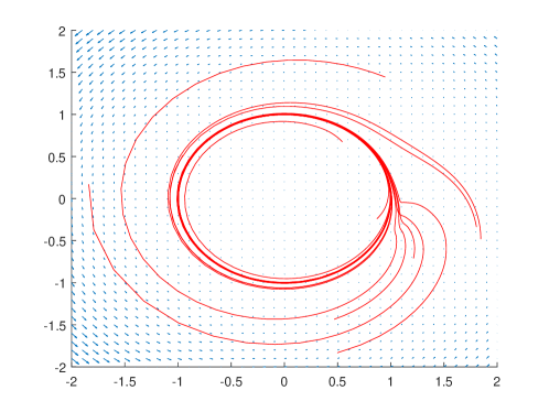
Figure 1: Vector field and trajectories with different initial points of dynamic system (2) that converges to $(1,0)$.

Remark 4.

Condition 2.1) is important. To see this, we can assume that $\mathcal{X}\subsetneq L_{\leq\alpha}$, by continuity of $L(x)$, there exists $x_{ext}\notin\mathcal{X}$ such that $L(x_{ext})\leq\alpha$. For any $x_{0}\in\mathcal{X}\setminus\mathcal{X}_{s}$, we can only ensure that the evaluation of $L(x)$ is decreasing, but it is possible to leave $\mathcal{X}$ heading towards $x_{ext}$. Note that our condition 2) in Theorem 2 only holds on $\mathcal{X}$, no stability guarantee can be given in this case.

Remark 5.

Theorem 2 is a generalization of the classical Lyapunov-Massera local asymptotic stability theorem, included in it as the case where $L$ is continuously differentiable and $\mathcal{X}_{s}=\{\mathbf{0}\}$. However we do not assume that $L\geq 0$ with equality only satisfied in $\mathbf{0}$, as $\mathbf{0}$ is already assumed LAS.

3.2 Piecewise Affine Lyapunov Function

PWA functions have strong modelling capability because they are dense in the space of continuous functions with a compact domain [36, Chapter 7.4]. This part will refine Theorem 2 to the Lipschitz continuous PWA Lyapunov function. For the sake of simplicity, we further assume

Assumption 3.

$\mathcal{X}$ is a polytope.

When $\mathcal{X}$ is not a polytope, it can be inner-approximated by a polytope up to arbitrary accuracy, thus this assumption will not limit the application of the proposed analysis. Additionally, it is worth noting that the definition of polytope used in this paper is not necessarily convex (see Section 2.2).

We now introduce our Lyapunov candidate under the form of a Lipschitz continuous PWA function. Let $\{C_{k}\}_{k=1}^{N_{C}}$ be an $N_{C}$-piece tessellation of $\mathcal{X}$ (i.e. $\cup_{k}C_{k}=\mathcal{X}$ and $\mathrm{int}(C_{k})\cap\mathrm{int}(C_{\ell})=\varnothing$ if $k\neq\ell$) where the $C_{k}$ are convex polytopes (without loss of generality we take $C_{1}\ni\mathbf{0}$). For $k\in\mathbb{N}_{N_{C}}$, we denote the vertices of $C_{k}$ by $\{v_{j,k}\}_{j=1}^{|C_{k}|}$. Using this structure, a PWA Lyapunov candidate $L_{\mathcal{X}}$ is defined on $\mathcal{X}$ by

$$\forall k\in\mathbb{N}_{N_{C}},x\in C_{k},\,L_{\mathcal{X}}(x)=g_{k}^{\top}x+b_{k}\;.$$ (4)

With appropriate conditions on $g_{k}\in\mathbb{R}^{n_{x}},b_{k}\in\mathbb{R}$, continuity of $L_{\mathcal{X}}$ on $\mathcal{X}$ is enforced: for any common vertex $v\in C_{k}\cap C_{\ell}$ (i.e. $\exists\;i\in\mathbb{N}_{|C_{k}|},\;j\in\mathbb{N}_{|C_{\ell}|}$ such that $v=v_{i,k}=v_{j,\ell}$), the condition

$$(g_{k}-g_{\ell})^{\top}v=b_{\ell}-b_{k}$$ (5)

should hold. Then, $L_{\mathcal{X}}$ is Lipschitz continuous on $\mathcal{X}$ with

$$\|L_{\mathcal{X}}\|_{\mathrm{Lip}}=|b_{1}|+\max_{1\leq k\leq N_{C}}\|g_{k}\|<\infty.$$

Remark 6.

Existence of a set $\{g_{k},b_{k}\}_{k=1}^{N_{C}}$ such that (4) defines a continuous function is guaranteed for any tessellation of $\mathcal{X}$, as a constant function on $\mathcal{X}$ always satisfies the continuity condition (i.e. $g_{k}=\mathbf{0},\;\forall\;k\in\mathbb{N}_{N_{C}}$ and $b_{i}=b_{j},\;\forall\;i,\;j\in\mathbb{N}_{N_{C}}$). When the tessellation is defined by a power-diagram, existence of convex PWA functions is further guaranteed [37].

Then, our PWA Lyapunov candidate $L_{\mathcal{X}}$ defined on $\mathcal{X}$ can be extended to the whole $\mathbb{R}^{n_{x}}$, such that Theorem 2 can be applied.:

$$L(x):=\begin{cases}\alpha+\eta\;\mathrm{dist}(x,\mathcal{X}),&\;x\in\mathbb{R}^{n_{x}}\setminus\mathcal{X}\\ L_{\mathcal{X}}(x),&\;x\in\mathcal{X}\end{cases}$$ (6)

where $\eta:=\max_{1\leq k\leq N_{C}}\|g_{k}\|$ is $L_{\mathcal{X}}$’s Lipschitz constant, and $\alpha\in\mathbb{R}$ is used to define the sublevel set (see Theorem 2) and can be tuned during the Lyapunov analysis.

Regarding our PWA LF candidate, the stability conditions in Theorem 2 can be restated as

Theorem 3.

Let Assumptions 1 to 3 hold, and consider the function $L_{\mathcal{X}}$ and $L$ defined by (4), (5) and (6). If $L$ moreover satisfies the following conditions

1. $\alpha$ is such that the evaluation of $L$ on the vertices satisfies

   $$\forall j,k\text{ s.t. }v_{j,k}\in\mathcal{X}\setminus\partial\mathcal{X}, L(v_{j,k})<\alpha$$ (7a)

   $$\forall j,k\text{ s.t. }v_{j,k}\in\partial\mathcal{X}, L(v_{j,k})=\alpha$$ (7b)

2. $\forall\;k\in\mathbb{N}_{N_{C}},\;\forall\;x\in C_{k}\cap(\mathcal{X}\setminus\mathcal{X}_{s}),$

   $$f(x)^{\top}g_{k}<0\;$$ (8)

Then $L$ is Lipschitz continuous and for all $x_{0}\in\mathrm{int}(\mathcal{X})$,

$$x(t|x_{0})\underset{t\to\infty}{\longrightarrow}\mathbf{0}.$$

Proof.

We first prove Lipschitz continuity of $L$. $L$ is Lipschitz continuous on $\mathcal{X}$ by its definition (5). By (6), as the distance function is $1$-Lipschitz, $L$ is Lipschitz continuous on $\mathbb{R}^{n}\setminus\mathcal{X}$ with same Lipschitz constant as in $\mathcal{X}$. Then, to prove global Lipschitz continuity of $L$ we only need to prove continuity at the boundary $\partial\mathcal{X}$, which is straightforward using condition (7b). Indeed, by construction of the $C_{k}$ and Assumption 3, any $x\in\partial\mathcal{X}$ is a convex combination of some vertices $v_{j,k}\in\partial\mathcal{X}$: $\exists\;k\in\mathbb{N}_{N_{C}},\{\lambda_{j}\}_{j=1}^{|C_{k}|}\subset[0,1]$ s.t.

$$v_{j,k}\in\mathrm{int}(\mathcal{X})\Rightarrow\lambda_{j}=0,\quad\sum_{j=1}^{|C_{k}|}\lambda_{j}=1,\quad\sum_{j=1}^{|C_{k}|}\lambda_{j}v_{j,k}=x$$

so that $L(x)=g_{k}^{\top}x+b_{k}=\sum_{j}\lambda_{j}\underset{\alpha}{\underbrace{(g_{k}^{\top}v_{j,k}+b_{k})}}=\alpha$, and $L=\alpha$ on $\partial\mathcal{X}$, which is consistent with the limit $\mathrm{dist}(x,\mathcal{X})\rightarrow 0$ in (6).

We are now going to use Theorem 2 to complete our proof. We first check condition 2.1) : $\mathcal{X}=L_{\leq\alpha}$. As $\mathcal{X}\supset L_{\leq\alpha}$ is trivially deduced from (6), we focus on the converse inclusion. Let $x\in\mathcal{X}$ and let us prove that $x\in L_{\leq\alpha}\text{ i.e. }L(x)\leq\alpha$.

By construction, $\exists\;k\in\mathbb{N}_{N_{C}}\text{ s.t. }x\in C_{k}$, and thus $\exists\{\lambda_{j}\}_{j=1}^{|C_{k}|}\subset[0,1]$ s.t. $\sum_{j}\lambda_{j}=1$ and $\sum_{j}\lambda_{j}v_{j,k}=x$. Again,

$$L(x)=\sum_{j=1}^{|C_{k}|}\lambda_{j}\,\underset{\leq\alpha}{\underbrace{(g_{k}^{\top}v_{j,k}+b_{k})}}\leq\alpha$$

using condition 3.1), which is the announced result.

We then move on to condition 2.2) in Theorem 2. Let $x\in\mathcal{X}\setminus\mathcal{X}_{s}$ and define $K(x):=\{k\in\mathbb{N}_{N_{C}}\;|\;x\in C_{k}\}$.

If $x\in\mathrm{int}(\mathcal{X})$ and $K(x)$ has a single element $k$, then $x\in\mathrm{int}(C_{k})$ and $L$ is smooth on a neighbourhood of $x$ with $\partial_{\mathrm{Cl}}L(x)=\{g_{k}\}$ and we conclude using condition 3.2).

Else, if $x\in\mathrm{int}(\mathcal{X})$ but $|K(x)|>1$, we deduce from the previous point and the definition of the Clarke gradient that

$$\partial_{\mathrm{Cl}}L(x)=\mathrm{co}\{g_{k}\;|\;k\in K(x)\}$$

so that $\forall\;y\in\partial\;L(x)$, $\exists\{\lambda_{k}\}_{k\in K(x)}\subset[0,1]$ s.t.

$$\sum_{k\in K(x)}\lambda_{k}=1\text{ and }\sum_{k\in K(x)}\lambda_{k}\,g_{k}=y.$$

This yields that for such $y$

$$f(x)^{\top}y=\sum_{k\in K(x)}\lambda_{k}\;\underset{<0}{\underbrace{f(x)^{\top}g_{k}}}<0$$

using condition 3.2).

Else, if $K(x)$ has a single element $k$ but $x\in\partial\mathcal{X}$ (i.e. $x$ is in the interior of a facet of $\mathcal{X}$), we notice that conditions (7a), (7b) enforce that $L$ is constant equal to $\alpha$ on $C_{k}\cap\partial\mathcal{X}$ and less than $\alpha$ in $\mathrm{int}(C_{k})$, which yields, using the definition (4), that $g_{k}$ is orthogonal to $\partial\mathcal{X}$ in $x$ and points outward of $\mathcal{X}$. Thus, the unit normal vector to $\partial\mathcal{X}\cap C_{k}$ at $x$ pointing outward of $\mathcal{X}$ is given by

$$\nu(x)=\frac{g_{k}}{\|g_{k}\|}.$$

Let $\epsilon>0$ and $x_{\epsilon}\in\mathbb{R}^{n_{x}}\setminus\mathcal{X}$ s.t. $\|x-x_{\epsilon}\|<\epsilon$. The definition (6) ensures that $L$ is differentiable in $x_{\epsilon}$ and that

$$\nabla L(x_{\epsilon})\underset{\epsilon\to 0}{\longrightarrow}\left(\max_{1\leq\ell\leq N_{C}}\|g_{\ell}\|\right)\nu(x)=\left(\max_{1\leq\ell\leq N_{C}}\|g_{\ell}\|\right)\frac{g_{k}}{\|g_{k}\|}.$$

denoting

$$\tilde{g}_{k}:=\left(\max_{1\leq\ell\leq N_{C}}\|g_{\ell}\|\right)\frac{g_{k}}{\|g_{k}\|}=\frac{\eta}{\|g_{k}\|}\,g_{k},$$

we then deduce that $\partial_{\mathrm{Cl}}L(x)=\mathrm{co}\{g_{k},\tilde{g}_{k}\}=[1,\eta/\|g_{k}\|]\,g_{k}$ and we conclude the proof using condition 3.2).

Eventually, in the last case where $|K(x)|>2$ and $x\in\partial\mathcal{X}$ (i.e. $x$ is on the boundary of a facet of $\mathcal{X}$), from the above we deduce that if $y\in\partial_{\mathrm{Cl}}L(x)$, then $\exists\{\lambda_{k}\}_{k\in K(x)},\{\mu_{k}\}_{k\in K(x)}\subset[0,1]$ s.t. $\sum_{k\in K(x)}\lambda_{k}+\mu_{k}=1$ and

$$y=\sum_{k\in K(x)}(\lambda_{k}\,g_{k}+\mu_{k}\,\tilde{g}_{k})=\sum_{k\in K(x)}(\lambda_{k}+\frac{\eta}{\|g_{k}\|}\,\mu_{k})\,g_{k}$$

and

$$f(x)^{\top}y=\sum_{k\in K(x)}(\lambda_{k}+\frac{\eta}{\|g_{k}\|}\,\mu_{k})\,\underset{<0}{\underbrace{f(x)^{\top}g_{k}}}<0$$

using condition 3.2). ∎

Finally, we would wrap up this part by sorting out the logic flow in this theorectical Section 3 again. The ultimate goal is to extend some prior knowledge of RoA (i.e. $\mathcal{X}_{s}$) to a bigger set $\mathrm{int}(\mathcal{X})$ via PWA continuous function, which is not smooth. Theorem 2 gives this characterization with respect to a continuous Lyapunov candidate via its Clarke gradient evaluation within the set $\mathcal{X}\setminus\mathcal{X}_{s}$. A specific characterization based on a continuous PWA Lyapunov candidate is then summarized in Theorem 3. This theorem is useful as it allows us to define the Lyapunov candidate only on the region of interest (i.e. $\mathcal{X}$), while the general Thereom 2 requires the definition of the Lyapunov candidate on the whole state space. Moreover, Theorem 3 reformulates the stability analysis into the analysis on function evaluation on the vertices and the negativity test on each affine piece. Additionally, this negativity test is local with respect to each affine piece, which implies that a local refinement of the Lyapunov candidate $L(x)$ is possible, further discussion of this aspect will be given at the end of the following section.

4 Learning Robust PWA Lyapunov Function

Recall the ultimate goal of this work; we would like to learn a PWA Lyapunov function for an unknown Lipschitz dynamic system $f(x)$ based on a given fixed dataset $D=\{x_{i},f_{i}\}_{i=1}^{N_{D}}$. Regarding the underlying dynamic system, we further assume that an overestimate of the Lipschitz constant is given:

Assumption 4.

$M$ is a known overestimate of the Lipschitz constant of $f$, i.e. for all $x,y\in\mathbb{R}^{n_{x}}$

$$\lVert f(x)-f(y)\rVert\leq M\lVert x-y\rVert.$$

Remark 7.

In the case where $\mathcal{F}$ is a Hilbert space with inner product $\langle\cdot;\cdot\rangle_{\mathcal{F}}$, it is also possible to work with another assumption that might be more convenient in some settings, but introduces additional technicalities in the learning process, namely: $M$ is a known overestimate of the Hilbert norm of $f$, i.e.

$$\|f\|_{\mathcal{F}}=\sqrt{\langle f;f\rangle_{\mathcal{F}}}\leq M.$$

In order to formulate a tractable learning problem, we further assume:

Assumption 5.

The tessellation of $\overline{\mathcal{X}\setminus\mathcal{X}_{s}}$ is fixed by a given set $\{C_{k}\}_{k=1}^{N_{C}}$.

The discussion about why we make this assumption is postponed to Remark 9. In this Section, we will show how to learn the PWA Lyapunov function on the tessellation $\{C_{k}\}_{k=1}^{N_{C}}$ based on Theorem 3. In the following subsections, we will gradually develop a Lyapunov function learning scheme under the form of an optimization problem.

Subsection 4.1 studies the negative condition for a general hypothesis space, and Subsection 4.2 studies the condition in the most basic hypothesis space, i.e. the Lipschitz function space.

4.1 Robust Lyapunov Condition

Although condition (8) is local to each affine piece, it still poses a numerically intractable infinite dimensional constraint, especially when the dynamic system is unknown and uncertain as $f\in\mathcal{F}$. In this subsection, we will show how this condition can be relaxed to a more tractable form via the calculus of the infimal convolution.

Based on dynamic evaluation $f_{i}:=f(x_{i})$ on location $x_{i}$ in the dataset $D$, the hypothesis space of the underlying dynamic system is tightened to

$$\mathcal{F}_{D}:=\{h\in\mathcal{F}\;|\;E_{x_{i}}h=f_{i},\forall\;i\in\mathbb{N}_{N_{D}}\}\;,$$ (9)

where $N_{D}$ is the number of the collected data points. Accordingly, we further define

$$\mathcal{F}_{D,i}:=\{h\in\mathcal{F}\;|\;E_{x_{i}}=f_{i}\}\;,$$ (10)

such that

$$\mathcal{F}_{D}=\cap_{i}\mathcal{F}_{D,i}\;.$$ (11)

The following theorem is the cornerstone representing the infinite dimensional Lyapunov constraint with a finite number of constraints.

Theorem 4.

The condition $0>g_{k}^{\top}f(x)$ holds for any $x\in C_{k}$ if there exist a set $\{\tilde{g}_{i,k}\}_{i=1}^{N_{D}}\subset\mathbb{R}^{n_{x}}$ such that

$$\begin{split}&\sum\limits_{i=1}^{N_{D}}\tilde{g}_{i,k}=g_{k},\;\text{and}\;\sum\limits_{i=1}^{N_{D}}\max\limits_{x\in C_{k}}\iota^{*}_{\mathcal{F}_{D,i}}(E_{x}^{*}\tilde{g}_{i,k})<0.\end{split}$$ (12)

Proof.

The key idea in this proof is to view the negativity condition (8) as an evaluation of a conjugate function in direction $g_{k}$:

$$0>\max_{x\in C_{k}}\ \max_{f\in\mathcal{F}_{D}}g_{k}^{T}f(x) \stackrel{{\scriptstyle(a)}}{{\Longleftrightarrow}}\; 0>\max_{x\in C}\ \max_{f\in\mathcal{F}}\ g_{k}^{T}(E_{x}f)-\iota_{\mathcal{F}_{D}}(f)$$

$$\stackrel{{\scriptstyle(b)}}{{\Longleftrightarrow}}\; 0>\max_{x\in C_{k}}\ \iota_{\mathcal{F}_{D}}^{*}(E_{x}^{*}g_{k})$$

$$\stackrel{{\scriptstyle(c)}}{{\Longleftrightarrow}}\; 0>\max_{x\in C_{k}}\ \iota_{\cap_{i}\mathcal{F}_{D,i}}^{*}(E_{x}^{*}g_{k})$$

$$\stackrel{{\scriptstyle(d)}}{{\Longleftrightarrow}}\; 0>\max_{x\in C_{k}}\ \left(\sum\limits_{i=1}^{N_{D}}\iota_{\mathcal{F}_{D,i}}(E_{x}^{*}g_{k})\right)^{*}$$

$$\stackrel{{\scriptstyle(e)}}{{\Longleftrightarrow}}\; 0>\max_{x\in C_{k}}\ \#_{i}\iota_{\mathcal{F}_{D,i}}^{*}(E_{x}g_{k})$$

$$\stackrel{{\scriptstyle(f)}}{{\Longleftrightarrow}}\; 0>\max_{x\in C_{k}}\ \inf_{\sum\tilde{g}_{i,k}=g_{k}}\sum\limits_{i}^{N_{D}}\iota_{\mathcal{F}_{D,i}}^{*}(E_{x}\tilde{g}_{i,k})$$

$$\stackrel{{\scriptstyle(g)}}{{\Longleftarrow}}\; 0>\inf_{\sum\tilde{g}_{i,k}=g_{k}}\max_{x\in C_{k}}\ \sum\limits_{i}^{N_{D}}\iota_{\mathcal{F}_{D,i}}^{*}(E_{x}\tilde{g}_{i,k})$$

$$\stackrel{{\scriptstyle(h)}}{{\Longleftrightarrow}}\; \exists\sum\limits_{i=1}^{N_{D}}\tilde{g}_{i,k}=g_{k}\text{ s.t. }\max_{x\in C_{k}}\sum\limits_{i}^{N_{D}}\iota_{\mathcal{F}_{D,i}}^{*}(E_{x}^{*}\tilde{g}_{i,k})<0.$$

$(a)$ writes the feasible set $\mathcal{F}_{D}$ into the objective function by indicator function, and $(b)$ follows the definition of the convex conjugate (see Section 2.1). $(c)$ applies the decomposition given in (11), and $(d)$ applies the calculus of indicator functions given in (1). $(e)$ applies calculus of conjugate function in Proposition 1, whose explicit form is written in $(f)$. $(g)$ applies the min-max inequality [38, Chapter 3.14]. Finally, as often performed in robust optimization (see e.g. [39]), the infimum operator is replaced by an existence assertion in $(h)$. ∎

The key concept behind Theorem 4 is the decomposition of the hypothesis space in (11). In particular, $\iota_{\mathcal{F}_{D,i}}^{*}(E_{x}^{*}\tilde{g}_{i,k})=\max_{f\in\mathcal{F}_{D,i}}g_{i,k}^{\top}f(x)$ is related to the uncertainty quantified from one data point, which usually has an easy-to-evaluate explicit closed solution. In comparison, the explicit solution is usually not available or difficult to evaluate when the whole dataset $D$ is considered. For example, when $\mathcal{F}$ is the space of Lipschitz functions, then the uncertainty boundary quantified by one data point defines a shifted cone. However, the uncertainty upper and lower bounds are PWA and non-trivial to evaluate [40] when the whole dataset $D$ is used. Recall Assumption 2, it is also reasonable to consider a reproducing kernel Hilbert space (RKHS), which underpins various uncertainty quantification methods such as Gaussian process regression [42] and deterministic error bound methods [43]. All these methods require computing the inverse of the Gram matrix or solving a second order cone program, which has an easy-to-evaluate explicit solution only when one data point is considered.

Remark 8.

In this work, we consider a decomposition of the hypothesis space $\mathcal{F}_{D}$ into the intersection of single-data models, i.e. $\mathcal{F}_{D}=\cap\mathcal{F}_{D,i}$. It is also possible to generalize the result to other decomposition, dubbed $\{\mathcal{F}_{j}\}$. If $\mathcal{F}=\cap_{j}\mathcal{F}_{j}$, where the conclusion in Theorem 4 needs slight modification accordingly:

$$\begin{split}&\sum\limits_{j}\tilde{g}_{j,k}=g_{k},\;0>\sum\limits_{j}\max\limits_{x\in C_{k}}\iota^{*}_{\mathcal{F}_{j}}(E_{x}^{*}\tilde{g}_{j,k})\;.\end{split}$$

Remark 9.

Even though function evaluation on a fixed location defines a linear operator from the hypothesis space $\mathcal{F}$ to $\mathbb{R}^{n_{x}}$, the mapping from the evaluation point to this operator is in general nonlinear. Assumption 5 is posed to develop a tractable formulation by avoiding this nonlinear mapping, and the next subsection will make use of this property. It is also noteworthy that, with a fixed tessellation, the parameters of the Lyapunov candidate on each affine piece (i.e. $g_{k},b_{k}$ on $C_{k}$) can be uniquely determined by the function evaluation on the vertices.

Another main benefit of a fixed tessellation is that it allows a direct control over the model complexity of the Lyapunov candidate. In particular, consider two Lyapunov candidates $L_{1}(x)$ and $L_{2}(x)$ with their corresponding partitions $\{C_{1,k}\}$ and $\{C_{2,k}\}$. Then, we can state that $L_{1}(x)$ is a refinement of $L_{2}(x)$ (i.e. $L_{1}(x)$ has a higher degree of modelling capability than $L_{2}(x)$) if $\forall\;C_{2,k},\;\exists\{C_{1,j}\}_{j\in\mathcal{I}_{k}}$ such that $\cup_{j}C_{1,j}=C_{2,k}$. As condition (8) is local to each affine piece, if one affine piece $C_{k}$ violates the assumptions of Theorem 4, then we can refine the model locally by further partition this piece.

4.2 A Convex Tractable Case: Lipschitz Dynamics

Theorem 4 gives us a representation of condition (8), but such a representation remains abstract and hard to check numerically; thus, we will now recast this representation under a tractable form, in a specific case. Although we have discussed that it is possible to consider a more complex function space property on top of the Lipschitz property in Section 4.1, this section will show that a convex learning problem exists even when we consider the most basic hypothesis space:

$$\mathcal{F}=\mathrm{Lip}(\mathcal{X})^{n_{x}}$$ (13)

In such case, the following corollary holds:

Corollary 5.

The condition $0>g_{k}^{\top}f(x)$ holds for any $x\in C_{k}$ if there exists a set $\{\tilde{g}_{i,k}\}_{i=1}^{N_{D}}\subset\mathbb{R}^{n_{x}}$ such that $\sum\limits_{i}\tilde{g}_{i,k}=g_{k}$ and for all $j\in\mathbb{N}_{|C_{k}|}$

$$\begin{split}&\sum\limits_{i=1}^{N_{D}}\tilde{g}_{i,k}^{\top}f_{i}+\lVert\tilde{g}_{i,k}\rVert M\lVert v_{j,k}-x_{i}\rVert<0.\end{split}$$ (14)

Proof.

$$\forall\;j,\; 0>\sum\limits_{i=1}^{N_{D}}\tilde{g}_{i,k}^{\top}f_{i}+\lVert\tilde{g}_{i,k}\rVert M\lVert v_{j,k}-x_{i}\rVert \stackrel{{\scriptstyle(a)}}{{\Longleftrightarrow}}\; 0>\max\limits_{x\in C_{k}}\sum\limits_{i=1}^{N_{D}}\tilde{g}_{i,k}^{\top}f_{i}+\lVert\tilde{g}_{i,k}\rVert M\lVert x-x_{i}\rVert$$ (15)

$$\stackrel{{\scriptstyle(b)}}{{\Longleftrightarrow}}\; 0>\max\limits_{x\in C_{k}}\sum\limits_{i=1}^{N_{D}}\max\limits_{y_{i}\in\mathcal{B}(f_{i},M\lVert x-x_{i}\rVert)}\tilde{g}_{i,k}^{\top}y_{i}$$

$$\stackrel{{\scriptstyle(c)}}{{\Longrightarrow}}\; 0>\max\limits_{x\in C_{k}}\sum\limits_{i=1}^{N_{D}}\max\limits_{f\in\mathcal{F}_{D,i}}\tilde{g}_{i,k}^{\top}f(x)$$

$$\stackrel{{\scriptstyle(d)}}{{\Longleftrightarrow}}\; 0>\max\limits_{x\in C_{k}}\sum\limits_{i=1}^{N_{D}}\iota^{*}_{\mathcal{F}_{D,i}}(E_{x}^{*}\tilde{g}_{i,k})\;.$$

To show $(a)$, we notice that the right-hand side of (15) is a convex maximization problem over a bounded convex polytope, its optimal solution is attained on its vertices, i.e. $\{v_{j,k}\}$. $(b)$ uses the Cauchy-Schwarz inequality on the second term of the sum $\tilde{g}_{i,k}^{\top}y_{i}=\tilde{g}_{i,k}^{\top}f_{i}+\tilde{g}_{i,k}^{\top}(y_{i}-f_{i})$. $(c)$ follows the assumption of Lipschitz constant overestimate (Assumption 4). Finally, $(d)$ applies the definition of the conjugate function. ∎

Remark 10.

If instead of Assumption 4, we suppose that $\|f\|_{\mathcal{F}}\leq M$, then one has a bound function $B_{M}:\mathbb{R}^{n_{x}}\rightarrow\mathbb{R}_{+}$ (depending on $M$) such that for any $x\in\mathbb{R}^{n_{x}}$, $h^{\star}\in\mathrm{argmin}_{h\in\mathcal{F}_{D}}\|h\|_{\mathcal{F}}$,

$$\|f(x)-h^{\star}(x)\|\leq B_{M}(x),$$

so that in the previous proof one has to replace $M\|x-x_{i}\|$ with $B_{M}(x)$. However, the problem here is that $B_{M}$ is not convex, so that relation $(b)$ does not hold anymore, and we would need other arguments (out of the scope of this article) to obtain a finite dimensional constraint.

Using Theorem 3 and Corollary 5, we get the following conditions for $\mathrm{int}(\mathcal{X})$ to be a positively invariant subset of the region of attraction of our unknown system:

$$\exists\;\{\tilde{g}_{i,k}\;|\;i\in\mathbb{N}_{N_{D}},k\in\mathbb{N}_{N_{C}}\}\subset\mathbb{R}^{n_{x}}, \exists\;\{g_{k}\;|\;k\in\mathbb{N}_{N_{C}}\}\subset\mathbb{R}^{n_{x}},$$

$$\exists\;\{b_{k}\;|\;k\in\mathbb{N}_{N_{C}}\}\subset\mathbb{R}, \exists\;\alpha\in\mathbb{R}$$

$$\forall\;k,\ell\in\mathbb{N}_{N_{C}},j\in\mathbb{N}_{|C_{k}|}\ \mathrm{s.t.}\ v_{j,k}\in C_{\ell}, (g_{k}-g_{\ell})^{\top}v_{j,k}=b_{\ell}-b_{k}$$ (5)

$$\forall\;k\in\mathbb{N}_{N_{C}},j\in\mathbb{N}_{|C_{k}|},\mathrm{s.t.}\ v_{j,k}\in\mathcal{X}\setminus\partial\mathcal{X} g_{k}^{\top}v_{j,k}+b_{k}<\alpha$$ (7a)

$$\forall\;k\in\mathbb{N}_{N_{C}},j\in\mathbb{N}_{|C_{k}|},\mathrm{s.t.}\ v_{j,k}\in\partial\mathcal{X} g_{k}^{\top}v_{j,k}+b_{k}=\alpha$$ (7b)

$$\forall\;k\in\mathbb{N}_{N_{C}}, \sum_{i=1}^{N_{D}}\tilde{g}_{i,k}=g_{k}$$ (12)

$$\forall\;k\in\mathbb{N}_{N_{C}},j\in\mathbb{N}_{|C_{k}|}, \sum\limits_{i=1}^{N_{D}}\tilde{g}_{i,k}^{\top}f_{i}+\lVert\tilde{g}_{i,k}\rVert M\lVert v_{j,k}-x_{i}\rVert<0.$$ (14)

Hence, our Lyapunov inference now boils down to a finite number of equality and strict inequality tests. Regarding condition (14) for a fixed $k\in\mathbb{N}_{N_{C}}$, we introduce slack variables to transform this certification problem into an optimization problem, with optimality giving the best robust certificates possible. This results in the following optimization problem:

$$s^{\star}_{\alpha,\epsilon}:=\min\limits_{\begin{subarray}{c}\{g_{k},b_{k}\},\{\tilde{g}_{i,k}\}\{s_{j,k}\}\end{subarray}} \sum{}_{k=1}^{N_{C}\vphantom{|C_{k}|}}\sum{}_{j=1}^{|C_{k}|}\;s_{j,k}$$

$$\forall\;k,\ell\in\mathbb{N}_{N_{C}},j\in\mathbb{N}_{|C_{k}|},\quad s_{j,k}\geq-\epsilon$$ (16a)

$$\hskip 20.00003pt\hskip 21.49997ptv_{j,k}\in C_{\ell}\Longrightarrow\quad (g_{k}-g_{\ell})^{\top}v_{j,k}=b_{\ell}-b_{k}$$ (16b)

$$\hskip 20.00003ptv_{j,k}\in\mathcal{X}\setminus\partial\mathcal{X}\Longrightarrow\quad g_{k}^{\top}v_{j,k}+b_{k}\leq\alpha-\epsilon$$ (16c)

$$\hskip 20.00003pt\hphantom{\mathcal{X}\setminus}\;\,v_{j,k}\in\partial\mathcal{X}\Longrightarrow\quad g_{k}^{\top}v_{j,k}+b_{k}=\alpha$$ (16d)

$$\sum{}_{i=1}^{N_{D}}\;\tilde{g}_{i,k}=g_{k}$$ (16e)

$$\sum{}_{i=1}^{N_{D}}\;\tilde{g}_{i,k}^{\top}f_{i}+\lVert\tilde{g}_{i,k}\rVert M\lVert v_{j,k}-x_{i}\rVert\leq s_{j,k}$$ (16f)

where $\epsilon>0$ is a user-defined negativity tolerance and $\alpha\in\mathbb{R}$ is the user-defined maximal value of the Lyapunov function. Constraint (16b) is the continuity condition, and constraint  (16c) is the interior condition (7a) and constraint (16d) is the boundary condition (7b), both stated in Theorem 3. When the slack variables satisfy $s_{j,k}<0$, constraints (16e) and (16f) correspond to the negative condition (8) stated in Theorem 3. Optimization problem (16) comes with the following result:

Theorem 6.

$\forall\;h\in\mathcal{F}$ whose function evaluations are consistent with the unknown underlying dynamic system $f$ ($h(x_{i})=f_{i},\;\forall\;x_{i},f_{i}\in D$), the solution to problem (16) defines a Lyapunov function for dynamic system $h$ on $\mathcal{X}$ when its optimal value verifies $s^{\star}_{\alpha,\epsilon}=-\epsilon\sum_{k=1}^{N_{C}}|C_{k}|$.

Proof.

We need to show that an optimal solution $\{g^{\mathrm{opt}}_{k},b^{\mathrm{opt}}_{k},\tilde{g}^{\mathrm{opt}}_{i,k},s^{\mathrm{opt}}_{j,k}\}$ satisfying

$$\sum_{j,k}\;s_{j,k}^{\mathrm{opt}}=-\epsilon\sum_{k}\;|C_{k}|$$

will also satisfy the conditions given in Theorem 3.

First of all, by constraint (16b) the learnt PWA function is continuous (see Equation (4)). On top of this, by constraints  (16d) and (16c), a solution to problem (16) recovers the condition 3.1) in Theorem 3. In the rest of this proof, we need to show that constraints (16e) and (16f) are equivalent to the negative condition 3.2) in Theorem 3 (i.e. $0>g_{k}^{\top}f(x),\;\forall\;x\in C_{k}$).

Note that, by $s_{j,k}\geq-\epsilon$ (constraint (16a)), the optimal value $\sum\limits_{j,k}s_{j,k}^{\mathrm{opt}}=-\epsilon\sum_{k=1}^{N_{C}}|C_{k}|$ implies that $s_{j,k}=-\epsilon,\;\forall\;j\in\mathbb{N}_{|C_{k}|},\;k\in\mathbb{N}_{N_{C}}$. Therefore, we have

$$0>-\epsilon\geq\sum\limits{i=1}^{N_{D}}\tilde{g}_{i,k}^{\top}f_{i}+M\lVert\tilde{g}_{i,k}\rVert\lVert v_{j,k}-x_{i}\rVert$$

$$\stackrel{{\scriptstyle(a)}}{{\Longrightarrow}}\; 0>\sum\limits_{i=1}^{N_{D}}\tilde{g}_{i,k}^{\top}f_{i}+M\lVert\tilde{g}_{i,k}\rVert\lVert v_{j,k}-x_{i}\rVert$$

$$\stackrel{{\scriptstyle(b)}}{{\Longrightarrow}}\; 0>g_{k}^{\top}h(x)\quad\forall\;x\in C_{k},\;h\in\mathcal{F}_{D}\;,$$

where $(a)$ holds by taking $\tilde{g}_{i,k}=\mathbf{0},\;\forall\;i$ such that $(x_{i},f_{i})\notin D$ and $(b)$ is Corollary 5. Based on this, we can derive:

In summary, constraints (16f) and (16e) guarantees the satisfaction of condition 3.2) in Theorem 3 for any $h\in\mathcal{F}_{D}$. Hence, we conclude the proof. ∎

The implication of this theorem is strong as it states that under the assumption of Lipschitz dynamics, we can learn/validate a LF by convex programming (16) even when the unknown underlying dynamic system $f$ is nonlinear.

Remark 11.

It is possible to adapt the proposed scheme (16) to the case where the measurements are contaminated by bounded measurement noise. More specifically, if the noisy measurement $\{\tilde{x}_{i},\tilde{f}_{i}\}$ is disturbed by measurement noise bounded by $\eta$ (i.e. the noise-free data lies at $\{x_{i},f_{i}\}$, such that $\lVert x_{i}-\tilde{x}_{i}\rVert\leq\eta$ and $\lVert f_{i}-\tilde{f}_{i}\rVert\leq\eta$). The constraint (16f) is accordingly modified to

$$\sum{}_{i=1}^{N_{D}}\;\tilde{g}_{i,k}^{\top}f_{i}+\lVert\tilde{g}_{i,k}\rVert\left(M\left(\lVert v_{j,k}-x_{i}\rVert+\eta\right)+\eta\right)\leq s_{j,k}\;.$$

For the sake of a clear presentation, we only consider the noise-free measurement in the rest of this paper.

Figure 2: Comparison between set membership method and the proposed method. The proposed scheme is evaluated by $\tilde{g}_{1}=0,\tilde{g}_{2}=0.65,\tilde{g}_{3}=0.35$.

4.3 Comparison with related works

We would like to wrap up this subsection by comparing the proposed learning scheme with other existing methods. In comparison with other PWA Lyapunov function based methods (see e.g. [29, 27]), the proposed scheme shows two major differences. First, the location of the samples and the tessellation of the PWA Lyapunov candidate are decoupled in the proposed scheme. While in existing methods, the data are sampled on the vertices of the tessellation, therefore, the data locations are usually structural due to the choice of the tessellation. Secondly, the robust Lyapunov stability conditions considered in the existing methods only consider the model uncertainty quantified by one data point. On the contrary, the proposed scheme synthetically makes use of the uncertainty quantified by each data point while maintaining a convex tractable structure.

Another framework related to the proposed approach is the set-membership method [40]. In short, the set-membership method models the set of Lipschitz functions whose evaluation on the points $\{x_{i}\}$ are consistent with data $\{x_{i},f(x_{i})\}$. The evaluation upper/lower bounds given by this method are PWA. To the best of our knowledge, even though the set-membership method could be extended to vector-valued functions, its typical applications are still limited to real-valued functions [44, 45] (i.e. $f(x)\in\mathbb{R}$). This is one major difference between the proposed scheme and the set-membership method. Now, we will show their difference regarding real-valued functions. To better demonstrate the difference, we consider a specific example in $\mathbb{R}$ (Figure 2), whose Lipschitz overestimate is set to $M=1$ and the data points are:

$$\{\left(0,f(0)=-0.4\right),\left(0.3,f(0.3)=-0.5\right),\left(1,f(1)=-0.6\right)\}$$

Now, consider a Lyapunov function candidate $L(x)=gx$ with $g=0.9$ within interval $[0,1]$. If the evaluation bounds of set-membership method are used, the Lyapunov decreasing condition needs to be examinated in all the sub-intervals generated by the PWA bounds (plotted as two-headed arrow in Figure 2). Determination of these sub-intervals is computationally heavy. Instead, if we hope to simplify the analysis by only taking one data point into consideration, none of the simple model generated by one data point can justify the Lyapunov decreasing condition (see black lines of different markers in Figure 2). These two aspects together imply the use of the whole dataset is necessary. The proposed scheme synthesizes the knowledge of simple models via a convex optimization. One optimal solution to the proposed scheme is plotted as a blue line in Figure 2, which only utilizes the last two points (i.e. $\tilde{g}_{1}=0$). It is worth noting that, in this example, if we only consider the left data and the right data point, the Lyapunov deceasing condition will fail even when the set-membership method is used. Hence, we can observe that the proposed method is able to search for the data points that are relevant to the Lyapunov decreasing condition. Additionally, this process is done by polynomial time convex optimization algorithms [46]. On the contrary, even though the set-membership method gives the tightest bound, checking the Lyapunov decreasing condition with these bounds is NP-hard, as it requires vertex elimination of the Voronoi cells.

Remark 12.

Note that in the proof of Theorem 5, we use the Cauchy-Schwarz inequality in (15), that holds only with Euclidean 2-norm. Actually, other norms can be considered, and the resulting problem (16) will have different properties accordingly. In particular, if 1-norm or $\infty$-norm is used, the resulting problem is a linear program. For the sake of simplicity, this paper uses the Euclidean norm only, and as a result, the learning problem (16) is a second order cone programming (SOCP) (Details in Section. 5).

5 Algorithm Development

After the introduction of the Lyapunov learning problem (16), we will discuss its learnability in Section 5.1. The original learning problem (16) will be recast to an equivalent but numerically more efficient form in Section 5.2. In the end, the main algorithms are summarized in Section 5.3.

5.1 Learnability

Above all, the set of Lyapunov functions is closed under positive scaling. More specifically, if a Lyapunov function $L(x)$ is learnt from problem (16), then its positive scaling $\lambda L(x)$ with $\lambda>0$ is also a Lyapunov function. Thus, the user-defined value $\alpha$ in (16c) will not introduce conservativeness in the learning problem. Furthermore, due to the introduction of the slack variables $\{s_{j,k}\}$, the learning problem (16) is always feasible. It is natural to ask the following core question in the limiting case:

If $\mathcal{X}$ is the RoA of the underlying dynamic system $f$ and we are allowed to evaluate the dynamic system $f$ in any finite set of points $x\in\mathcal{X}$, can we always learn a Lyapunov function for any RoA subsets $\mathcal{X}\setminus\mathcal{X}_{s}$?

Unfortunately, the answer to this question is no, and a counterexample is summarized in the following Corollary:

Corollary 7.

Let Assumption 1 hold and let the hypothesis space $\mathcal{F}$ satisfy Equation (13), if $\mathbf{0}\notin\mathrm{int}(\mathcal{X}_{s})$, then the optimal value to problem (16) verifies:

$$\sum\limits_{j,k}s_{j,k}^{\mathrm{opt}}>-\epsilon\sum_{k=1}^{N_{C}}|C_{k}|$$

Proof.

Note that the user-defined tolerance is negative (i.e. $-\epsilon<0$) and arbitrary, we need to show that there exist one $s_{j,k}^{\mathrm{opt}}\geq 0$ in the optimal solution.

By Assumption 1, we have $f(\mathbf{0})=\mathbf{0}$. Using the Lipschitz condition and Assumption 4 yields

$$\lVert f_{i}\rVert =\lVert f_{i}-\mathbf{0}\rVert\leq M\lVert x_{i}-\mathbf{0}\rVert$$

As $\mathbf{0}$ is the LAS EP, we have $\mathbf{0}\in\mathcal{X}_{s}$, and by assumption $\mathbf{0}\notin\mathrm{int}(\mathcal{X}_{s})$, so $\mathbf{0}\in\partial\mathcal{X}_{s}$. Consider the affine piece $C_{k}$ that contains $\mathbf{0}$ (i.e. $\mathbf{0}\in C_{k}$ and it is a vertex of $C_{k}$). By inspecting the constraint (14) and using Cauchy-Schwarz inequality, one has:

$$\tilde{g}_{i,k}^{\top}f_{i}+M\lVert\tilde{g}_{i,k}\rVert\lVert\mathbf{0}-x_{i}\rVert$$

$$\geq M\lVert\tilde{g}_{i}\rVert\lVert\mathbf{0}-x_{i}\rVert-\lVert\tilde{g}_{i}\rVert\lVert f_{i}\rVert\geq 0\;.$$

Thus, the constraint (16f) will become:

$$s_{j,k}\geq\sum\limits_{i=1}^{N_{D}}\tilde{g}_{i,k}^{\top}f_{i}+M\lVert\tilde{g}_{i,k}\rVert\lVert v_{j,k}-x_{i}\rVert\geq 0>-\epsilon,$$

which is sufficient to conclude the proof. ∎

Even though our theory of expanding a-priori knowledge from $\mathcal{X}_{s}$ to a bigger set $\mathcal{X}$ holds for any $\mathcal{X}_{s}$ (Section 3), Corollary 7 shows that, if the domain of a Lyapunov function contains $\mathbf{0}$, then it is impossible to learn this function by only assuming Lipschitz continuity (Equation (13)). Similar observation of infeasibility was also made in the constructive proof of converse Lyapunov theorem [47]. Meanwhile, many numerical methods also have similar limitation around the invariant set [48, Chapter 2.11]; we refer the interested reader to [49, 50] for more details. In summary, if we do not further assume other function space structure on the hypothesis space $\mathcal{F}$, following assumption is required to ensure the learnability of problem (16):

Assumption 6.

$\mathbf{0}\in\mathrm{int}(\mathcal{X}_{s})\;.$

We would stress again that the assumption above is only necessary for the learning scheme based on problem (16), and a learning scheme without this assumption is left for future research.

After answering the aforementioned problem by Corollary 7, the follow-up core question is:

Given an RoA prior estimate $\mathcal{X}_{s}$, what condition on dataset $D$ should hold to enable learning the PWA Lyapunov function on $\mathcal{X}\setminus\mathcal{X}_{s}$?

Obviously, it is impossible to answer this question with a sufficient condition, regarding the arbitrariness of the unknown dynamic system $f$. However, if we only assume the function space to be Lipschitz (Equation (13)), we can still give an initial check of the learnability of problem (16). In order to discuss this necessary condition, we first define

$$r_{i}:=\frac{\lVert f_{i}\rVert}{M}\;.$$

We state the necessary condition as follows:

Lemma 8.

Let Assumption 1 hold and let hypothesis space $\mathcal{F}=\mathrm{Lip}(\mathcal{X})^{n_{x}}$. If solutions to problem (16) define a Lyapunov function as in Theorem 3, then $\mathcal{X}\setminus\mathcal{X}_{s}\subset\cup_{i=1}^{N_{D}}\mathcal{B}(x_{i},r_{i})$.

Proof.

From the proof of Theorem 6, the solution to problem (16) is a Lyapunov function if for $\forall\;k\in\mathbb{N}_{N_{C}},\;j\in\mathbb{N}_{|C_{k}|}$, $s_{j,k}=-\epsilon$. Let $x\in\mathcal{X}\setminus\mathcal{X}_{s}$, and without loss of generality, we suppose $x\in C_{k}$ for some $k\in\mathbb{N}_{N_{C}}$. By Corollary 5,

$$0>-\epsilon=s_{j,k}\geq\sum\limits{i=1}^{N_{D}}\tilde{g}_{i,k}^{\top}f_{i}+M\lVert\tilde{g}_{i,k}\rVert\lVert x-x_{i}\rVert\;,$$

which implies that there exist at least one $n\in\mathbb{N}_{N_{d}}$ such that

$$0>\tilde{g}_{n,k}^{\top}f_{n}+M\lVert\tilde{g}_{n,k}\rVert\lVert x-x_{n}\rVert$$

$$\ \Longrightarrow \lvert\tilde{g}_{n,k}^{\top}f_{n}\rvert>M\lVert\tilde{g}_{n,k}\rVert\lVert x-x_{n}\rVert$$

$$\stackrel{{\scriptstyle(a)}}{{\Longrightarrow}} \lVert f_{n}\rVert\lVert\tilde{g}_{n,k}\rVert>M\lVert\tilde{g}_{n,k}\rVert\lVert x-x_{n}\rVert$$

$$\Longleftrightarrow x\in\mathcal{B}\left(x_{n},\frac{\lVert f_{n}\rVert}{M}\right)$$

$$\Longleftrightarrow x\in\mathcal{B}(x_{n},r_{n})$$

$$\Longrightarrow x\in\cup_{i=1}^{N_{D}}\mathcal{B}(x_{i},r_{i})$$

where $(a)$ follows from the Cauchy-Schwarz inequality. Due to the inclusion condition is sastisfied for any point $x\in\mathcal{X}\setminus\mathcal{X}_{s}$, we conclude the proof with $\mathcal{X}\setminus\mathcal{X}_{s}\subset\cup_{i}^{N_{D}}\mathcal{B}(x_{i},r_{i})$. ∎

This lemma shows the connection between learning a PWA Lyapunov function and the set covering problem, which was proved to be equivalent to a non-convex semi-infinite problem [51], and thus one should not try to check the condition in Lemma 8 numerically. Recall a key idea behind the problem (16): the global analysis on $\mathcal{X}\setminus\mathcal{X}_{s}$ is reduced to the analysis on the vertices. This inspires us to relax the continuous set covering problem to the covering problem of the vertices and we state this condition in the following Corrolary

Corollary 9.

Let Assumption 1 hold and let hypothesis space $\mathcal{F}=\mathrm{Lip}(\mathcal{X})^{n_{x}}$, if solutions to problem (16) define a Lyapunov function as in Theorem 3, then

$$\{v_{i,k}\}_{\begin{subarray}{c}1\leq k\leq N_{C}\\ 1\leq i\leq|C_{k}|\end{subarray}}\subset\cup_{i=1}^{N_{D}}\mathcal{B}(x_{i},r_{i})\;,$$ (17)

This necessary condition (17) can be checked in polynomial time. If this test fails, it means that there exist $v_{i,k}\notin\cup_{i=1}^{N_{D}}\mathcal{B}(x_{i},r_{i})$, and therefore, the data is not informative enough to learn a PWA Lyapunov function by only assuming the Lipschitz condition (Equation (13)). Accordingly, the learning process will be terminated. Intuitively, the points which $v_{i,k}\notin\cup_{i=1}^{N_{D}}\mathcal{B}(x_{i},r_{i})$ should suggest the location where additional samples are required. We leave the investigation about this aspect for future work.

5.2 Computationally efficient recasting

In this part, we will discuss how we recast the original problem (16) to an equivalent problem that can be handled numerically more efficiently.

Data Refinement
One main computational bottleneck for the original problem (16) comes from the number of decision variables. Without loss of generality, we consider an affine piece $C_{k}$. By inspecting the tessellation validation test (17), if a data point $(x_{i},f(x_{i}))$ does not contain any vertices of $C_{k}$ in $\mathcal{B}(x_{i},r_{i})$ (i.e. $C_{k}\ni v_{j,k}\notin\mathcal{B}(x_{i},r_{i})$), then $\forall\;\tilde{g}\in\mathbb{R}^{n_{x}}$, following inequality holds

$$0\leq\tilde{g}^{\top}f_{i}+M\lVert\tilde{g}\rVert\lVert v_{j,k}-x_{i}\rVert\;.$$

Hence, this data point $x_{i}$ cannot help enforce the strict negative Lyapunov decreasing condition (16f), and can therefore be neglected in the constraints defined on affine piece $C_{k}$. Accordingly, the set of data points relevant to $C_{k}$ are:

$$D_{k}:=\left\{(x_{i},f_{i})\;\middle|\;i\in I_{k}\right\}\quad\text{with}\quad I_{k}:=\left\{i\in\mathbb{N}_{N_{D}}\;\middle|\;\exists\;j\in\mathbb{N}_{|C_{k}|},\;v_{j,k}\in\mathcal{B}(x_{i},r_{i})\right\}$$

The condition defining this set essentially states the point should at least be possible to enforce strict negativity on constraint (16f) at one vertex. This technique can significantly reduce the computational cost. To see this, we consider a homogeneous tessellation within a unit hypercube centred at $\mathbf{0}$ within which data points scatter uniformly. We further assume that the affine pieces of the tessellation are hypercubes with edge width $rel$. Based on the Lipschitz condition (13), each data point will at most get involved in $O\left(\left(\frac{r_{i}}{rel}\right)^{n_{x}}\right)\ll N_{C}$. Notice that $r_{i}\leq.5$ (see Section 5.1), the number of decision variables are reduced to roughly $O\left(\frac{1}{2^{n_{x}}}\right)$ of the problem defined by the whole data set. In the numerical example we consider in Section 6, we observe on average an 81% reduction in the number of decision variables, which makes the problem tractable on a Laptop without memory overflow.

Explicit SOCP formualtions
In the numerical implementation, it is critical to convert the inequality constraint (16f) into a set of second-order cones, or Lorentz cone in particular [38]:

$$s_{j,k}\geq \sum_{i\in I_{k}}\;\tilde{g}_{i,k}^{\top}f_{i}+t_{i,j,k}$$

$$t_{i,j,k} \geq\lVert\tilde{g}_{i,k}\rVert M\lVert v_{j,k}-x_{i}\rVert\;,$$

where $|I_{k}|$ auxiliary decision scalar variables $\{t_{i,j,k}\}$ are introduced per vertex $v_{j,k}$ in order to define the Lorentz cone. The resulting computational complexity per iteration in an interior point algorithm is $O(N_{D}N_{C}n_{x}^{2})$ [52]. In comparison, without this reformulation, this inequality constraint will be directly handled by a block diagonal positive semi-definite matrix, whose computational complexity per iteration in an interior point algorithm is $O\left(|C_{k}|\left(N_{D}n_{x}\right)^{3}\right)$ [53, Chapter 1].

The Recast Problem
After introducing of the reformulation techniques, the learning problem we solved becomes:

$$s^{\star}_{\alpha,\epsilon}:=\min\limits_{\begin{subarray}{c}\{g_{k},b_{k}\},\{\tilde{g}_{i,k}\}\\ \{s_{j,k}\},\{t_{i,j,k}\}\end{subarray}} \sum{}_{k=1}^{N_{C}\vphantom{|C_{k}|}}\sum{}_{j=1}^{|C_{k}|}\;s_{j,k}$$ (18a)

$$\forall\;k,\ell\in\mathbb{N}_{N_{C}},j\in\mathbb{N}_{|C_{k}|},\quad s_{j,k}\geq-\epsilon$$ (18b)

$$\hskip 20.00003pt\hskip 21.49997ptv_{j,k}\in C_{\ell}\Longrightarrow\quad (g_{k}-g_{\ell})^{\top}v_{j,k}=b_{\ell}-b_{k}$$ (18c)

$$\hskip 20.00003ptv_{j,k}\in\mathcal{X}\setminus\partial\mathcal{X}\Longrightarrow\quad g_{k}^{\top}v_{j,k}+b_{k}\leq\alpha-\epsilon$$ (18d)

$$\hskip 20.00003pt\hphantom{\mathcal{X}\setminus}\;\,v_{j,k}\in\partial\mathcal{X}\Longrightarrow\quad g_{k}^{\top}v_{j,k}+b_{k}=\alpha$$ (18e)

$$\sum{}_{i\in I_{k}|}\;\tilde{g}_{i,k}=g_{k}$$ (18f)

$$\sum{}_{i\in I_{k}|}\;\tilde{g}_{i,k}^{\top}f_{i}+t_{i,j,k}\leq s_{j,k}$$ (18g)

$$\forall i\in I_{k},\quad \lVert\tilde{g}_{i,k}\rVert M\lVert v_{j,k}-x_{i}\rVert\leq t_{i,j,k}$$ (18h)

Remark 13.

Learning without knowing $M$: It is possible to consider $M$ as a decision variable, and determine the largest Lipschitz constant for which a Lyapunov function can be found given a particular set of data. More specifically, constraint (18h) is recast to a positive semi-definite constraint by

$$\begin{bmatrix}MI_{n_{x}}&\tilde{g}_{i,k}\\ \tilde{g}_{i,k}^{\top}&t_{i,j,k}\end{bmatrix}\in\mathcal{S}^{+}\;,$$ (19)

where $\mathcal{S}^{+}$ denotes the set of positive semi-definite matrices. However, once this formulation is used, the resulting optimization problem becomes a semidefinite programming (SDP) and the data refinement technique proposed at the beginning of this Section 5.2 cannot be applied. Even though the particular sparsity structure in (19) can be exploited to improve the computational efficiency, the computational cost of this optimization still drastically increase in comparison with the SOCP problem (16).

5.3 Algorithms

The final learning algorithm is summarized in Algorithm 1. Even though we use the standard tessellation algorithm in algorithm 1, generating a good tessellation is vital but non-trivial. Existing works mostly focus on the link between a convex liftable tessellation and the power diagram (see e.g. [54, 55]). However, as the Lyapunov function studied in this paper is not necessarily convex, hence we leave the study of this topic in the future research. And we use the standard Delaunay triangulation in this work [56].

Algorithm 1   

Input: RoA prior $\mathcal{X}_{s}$, negativity tolerance $-\epsilon$, Lipschitz overestimate $M$, set level $\alpha$,
    Output: Lyapunov function $L(x)$

  Refine a tessellation $\{C_{k}\}_{k=1}^{N_{c}}$ until it satisfies (17)

  if tessellation is valid then

     Solve optimization (18)

     if Optimal value solution satisfies $s^{\star}_{\alpha,\epsilon}=-\epsilon\sum_{k=1}^{N_{C}}|C_{k}|$ then

        Return

     end if

  else

     Return cannot learn $L(x)$.

  end if

Sequential Space Partition
Based on the aforementioned strategies, the scalbility of the learning problem (16) can still be improved by partitioning the region of interest $\mathcal{X}$ into a sequence of subset, such that

$$\mathcal{X}_{s}\subset\mathcal{X}_{1}\subset\mathcal{X}_{2}\dots\subset\mathcal{X}\;.$$

Note that the logic behind the proposed algorithm is an augmentation of the a-priori knowledge in $\mathcal{X}_{s}$ to $\mathcal{X}$, this allows us to further improve the computational efficiency. The key idea is to gradually augment the volume of the RoA, and in each iteration, it is only necessary to learn the LF on the set $\mathcal{X}_{i}\setminus\mathcal{X}_{i-1}$. This sequential learning algorithm is summarized in Algorithm 2. It is noteworthy that, if one needs to recover the whole LF on $\mathcal{X}\setminus\mathcal{X}_{s}$, then it is necessary to impose the continuity condition on be boundary of $\partial\mathcal{X}_{i}$ between the $i$-th iteration and the $i+1$-th iteration. The corresponding algorithm is summarized in Algorithm 2.

Algorithm 2   

Input: Subset sequence $\{\mathcal{X}_{i}\}$ and the initial basin $\mathcal{X}_{0}=\mathcal{X}_{s}$
    Output: Lyapunov function $L(x)$

  $i=1$

  while $\{\mathcal{X}_{s}\neq\mathcal{X}\}$ do

     Run Algorithm. 1 with $\mathcal{X}_{s}$

     if Algorithm 1 failed then

        Return cannot learn $L(x)$.

     end if

     $i\leftarrow i+1$

     $\mathcal{X}_{s}\leftarrow\mathcal{X}_{i}$

  end while

5.4 Learning $\mathcal{X}$

Up to this point, we assume knowledge of $\mathcal{X}$ within which the stability analysis is conducted. However, such prior knowledge/assumption is not necessarily available. Instead, the users may only have access to a set of data and hope to find out a ROA based on this dataset. In this case, we will need to solve the Learning problem (16) without the boundary condition:

$$\begin{split}s^{\star}_{\epsilon}:=\min\limits_{\begin{subarray}{c}\{g_{k},b_{k}\},\{\tilde{g}_{i,k}\}\{s_{j,k}\}\end{subarray}}&\sum{}_{k=1}^{N_{C}\vphantom{|C_{k}|}}\sum{}_{j=1}^{|C_{k}|}\;s_{j,k}\\ \forall\;k,\ell\in\mathbb{N}_{N_{C}},j\in\mathbb{N}_{|C_{k}|},\quad&s_{j,k}\geq-\epsilon\\ \hskip 20.00003pt\hskip 21.49997ptv_{j,k}\in C_{\ell}\Longrightarrow\quad&(g_{k}-g_{\ell})^{\top}v_{j,k}=b_{\ell}-b_{k}\\ \hskip 20.00003ptv_{j,k}\in\mathcal{X}\setminus\partial\mathcal{X}\Longrightarrow\quad&g_{k}^{\top}v_{j,k}+b_{k}\leq\alpha-\epsilon\\ &\sum{}_{i=1}^{N_{D}}\;\tilde{g}_{i,k}=g_{k}\\ &\sum{}_{i=1}^{N_{D}}\;\tilde{g}_{i,k}^{\top}f_{i}+\lVert\tilde{g}_{i,k}\rVert M\lVert v_{j,k}-x_{i}\rVert\leq s_{j,k}\end{split}$$ (20)

Based on the solution to this problem, it is possible to determine a ROA by the following Corollary:

Corollary 10.

If the solution to problem (20) satisfies $s^{\star}_{\epsilon}=-\epsilon\sum_{k=1}^{N_{C}}|C_{k}|$, then any sublevel set $L_{\leq\alpha}\subset\mathcal{X}$ with $\alpha\in\mathbb{R}$ is attracted to $0$ under the unknown dynamics $f$.

Proof.

If the solution to (20) satisfies $s^{\star}_{\epsilon}=-\epsilon\sum_{k=1}^{N_{C}}|C_{k}|$, by choosing $\alpha\in\mathbb{R}$ such that $L_{\leq\alpha}\subset\mathcal{X}$, then the optimal solution to (20) is also an optimal solution to:

$$\min\limits_{\begin{subarray}{c}\{g_{k},b_{k}\},\{\tilde{g}_{i,k}\}\{s_{j,k}\}\end{subarray}} \sum{}_{k=1}^{N_{C}\vphantom{|C_{k}|}}\sum{}_{j=1}^{|C_{k}|}\;s_{j,k}$$

$$\forall\;k,\ell\in\mathbb{N}_{N_{C}},j\in\mathbb{N}_{|C_{k}|},\quad s_{j,k}\geq-\epsilon$$

$$\hskip 20.00003pt\hskip 21.49997ptv_{j,k}\in C_{\ell}\cap L_{\leq\alpha}\Longrightarrow\quad (g_{k}-g_{\ell})^{\top}v_{j,k}=b_{\ell}-b_{k}$$

$$\hskip 20.00003ptv_{j,k}\in L_{\leq\alpha}\setminus\partial L_{\leq\alpha}\Longrightarrow\quad g_{k}^{\top}v_{j,k}+b_{k}\leq\alpha-\epsilon$$

$$\hskip 20.00003pt\hphantom{\mathcal{X}\setminus}\;\,v_{j,k}\in\partial L_{\leq\alpha}\Longrightarrow\quad g_{k}^{\top}v_{j,k}+b_{k}=\alpha$$

$$\sum{}_{i=1}^{N_{D}}\;\tilde{g}_{i,k}=g_{k}$$

$$\sum{}_{i=1}^{N_{D}}\;\tilde{g}_{i,k}^{\top}f_{i}+\lVert\tilde{g}_{i,k}\rVert M\lVert v_{j,k}-x_{i}\rVert\leq s_{j,k}\;,$$

whose tessellation is given by $\{C_{k}\cap L_{\leq\alpha}\}_{k}^{N_{C}}$. Hence, Theorem 6 holds in $L_{\leq\alpha}$, which summarizes the proof.

∎

Based on this corollary, we are able to learn the ROA within $\mathcal{X}$ by applying the algorithm summarized in Algorithm 3.

Algorithm 3   

Input: RoA prior $\mathcal{X}_{s}$, negativity tolerance $-\epsilon$, Lipschitz overestimate $M$,
    Output: Lyapunov function $L(x)$, ROA $L_{\leq\alpha}$

  Refine a tessellation $\{C_{k}\}_{k=1}^{N_{c}}$ until it satisfies (17)

  if tessellation is valid then

     Solve optimization (20)

     if Optimal value solution satisfies $s^{\star}_{\epsilon}=-\epsilon\sum_{k=1}^{N_{C}}|C_{k}|$ then

        find $\alpha\in\mathbb{R}$ such that $L_{\leq\alpha}\subset\mathcal{X}$

        Return

     end if

  else

     Return cannot learn $L(x)$.

  end if

6 Numerical Results

In this part, we going to evaluate the proposed learning schemes in two different examples. In particular, we will make use of Algorithm 1, 2 and 3 in the first example and use Algorithm 3 in the second one. All the following results are implemented on a laptop with Intel i7-11800H and 32G memory, and the Mosek is used for solving the SOCP problem.

6.1 Non Polynomial dynamic system

We consider a two-dimensional nonlinear dynamic system:

$$\dot{x}_{1}(t)= -0.9\sin(x_{1}(t))\cos(x_{2}(t))+0.2x_{1}(t)x_{2}(t)+0.25x_{2}(t)^{2}$$

$$\dot{x}_{2}(t)= -1\sin(x_{2}(t))(|x_{1}(t)+0.2|)+0.5\frac{x_{1}(t)x_{2}(t)}{\cos(x_{2}(t))-0.3x_{1}(t)}$$

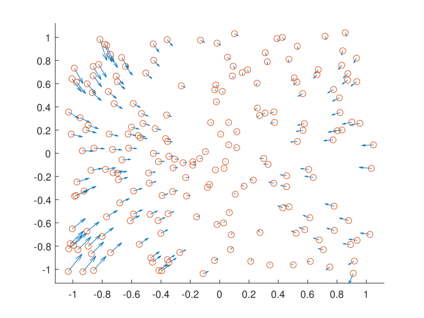
(a) The data used for the learning scheme.

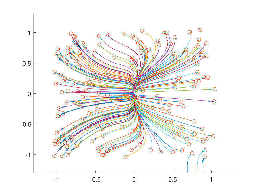
(b) Underlying dynamics (not used for learning).

Figure 3: Representations of the considered nonpolynomial dynamic system.

We assume that we know a ROA $\mathcal{X}_{s}=[-0.1,0.1]^{2}$. A dataset with only 200 samples within $[-1,1]^{2}\subset\mathbb{R}^{2}$ is used to learn the underlying Lyapunov function: the positions $\{x_{i}\}$ and speeds $\{f(x_{i})\}$ of these samples are plotted in Figure 3(a), from which we can observe that this dataset is relatively sparse in $[-1,1]^{2}$. Judging by the speed sample, the dynamic system seem stable within the box $[-0.4,0.4]^{2}$, while stability within the region $[-1,1]^{2}\setminus[-0.4,0.4]^{2}$ is unclear because of the speed samples in the lower right corner in Figure 3(a). Hence, we ran sequential space partition scheme (Algorithm 2). In particular, we first use Algorithm 1 in the region $[-0.4,0.4]^{2}$ with $\mathcal{X}_{s}=[-0.1,0.1]^{2}$. After we justify that $[-0.4,0.4]^{2}$ is a positively invariant subset of the ROA, then we further apply Algorithm 3 to $[-1,1]^{2}$ with $\mathcal{X}_{s}=[-0.4,0.4]^{2}$. In both sub-problems, the negativity tolerances $\epsilon$ are set to $10^{-3}$ and the tessellation are both randomly generated by Delaunay triangulation [56].

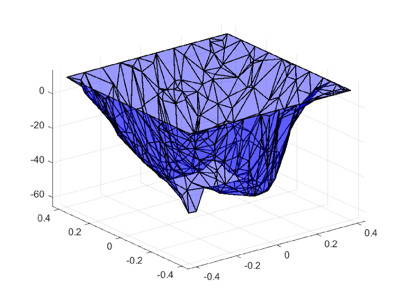
(a) $\mathcal{X}_{s}=[-0.1,0.1]^{2}\subset\mathcal{X}=[-0.4,0.4]^{2}$.

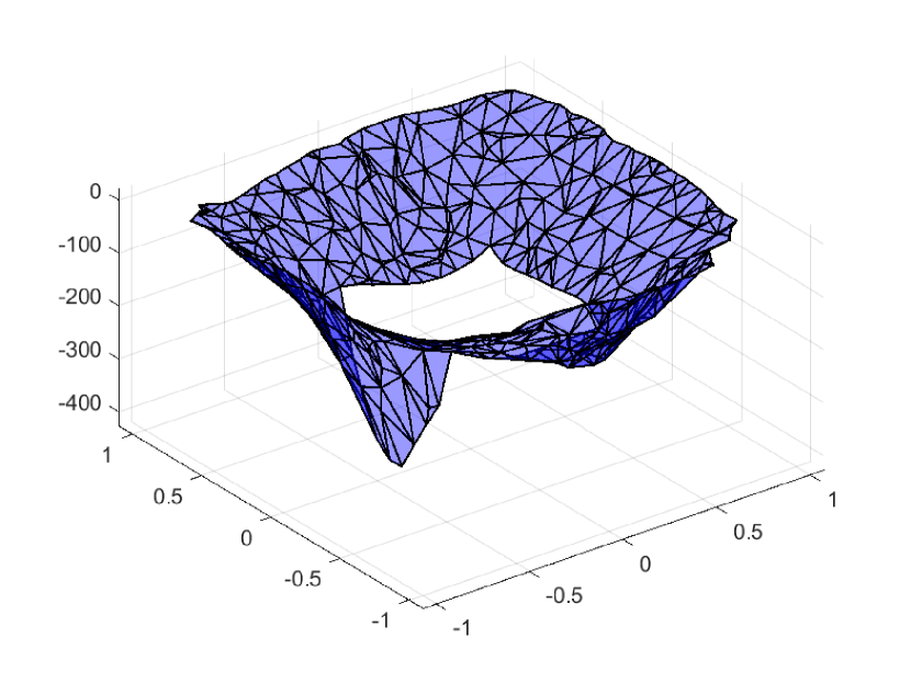
(b) Learning a ROA estimate within $[-1,1]^{2}$.

Figure 4: Visualization of the learnt Lyapunov functions.

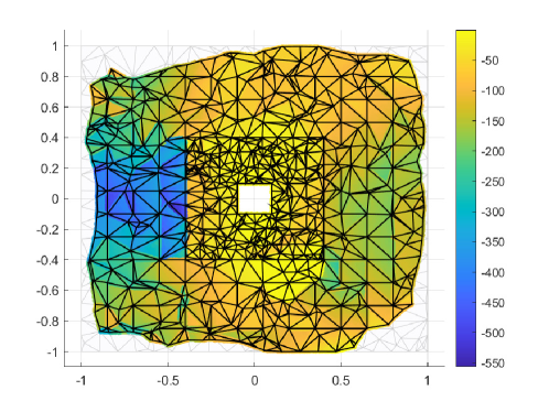
Figure 5: Evaluation of $f(x)^{\top}\partial_{\rm Cl}L(x)$ on the learnt ROA, the gray triangulation in the background is the tessellation used to solve Problem (20), while the coloured region in the front is our ROA estimate.

The learnt Lyapunov function in $[-0.4,0.4]^{2}$ is shown in Figure 4(a), while the ROA we finally end up with is shown in Figure 5. Moreover, the Lyapunov function learnt from Algorithm 3 in $\mathcal{X}_{s}=[-1,1]^{2}\setminus[-0.4,0.4]^{2}$ is shown in Figure 4(b). Figure 5 also shows the evaluation of $f(x)^{\top}\partial_{\rm Cl}L(x)$ with respect to the underlying dynamic system, whose maximal evaluation is $-1.525\times 10^{-2}<0$, as expected from a Lyapunov function. In accordance with our guess, the learnt ROA in Figure 5 cuts off the lower right corner, because this region does not seem to be stable. To see that, we simulate the underlying dynamic system by setting the initial states to points in our dataset. The simulated trajectories are plotted in Figure 3(b); please note that these trajectories are not used in the learning scheme at all.

6.2 Reverse Time Van Del Pol Oscillator

In this part, we consider the reverse time Van Del Pol oscillator:

$$\dot{x}_{1}(t) =-2x_{2}(t)$$

$$\dot{x}_{2}(t) =-0.8x_{1}(t)-10(x_{1}(t)^{2}-0.21)x_{2}(t)\;.$$

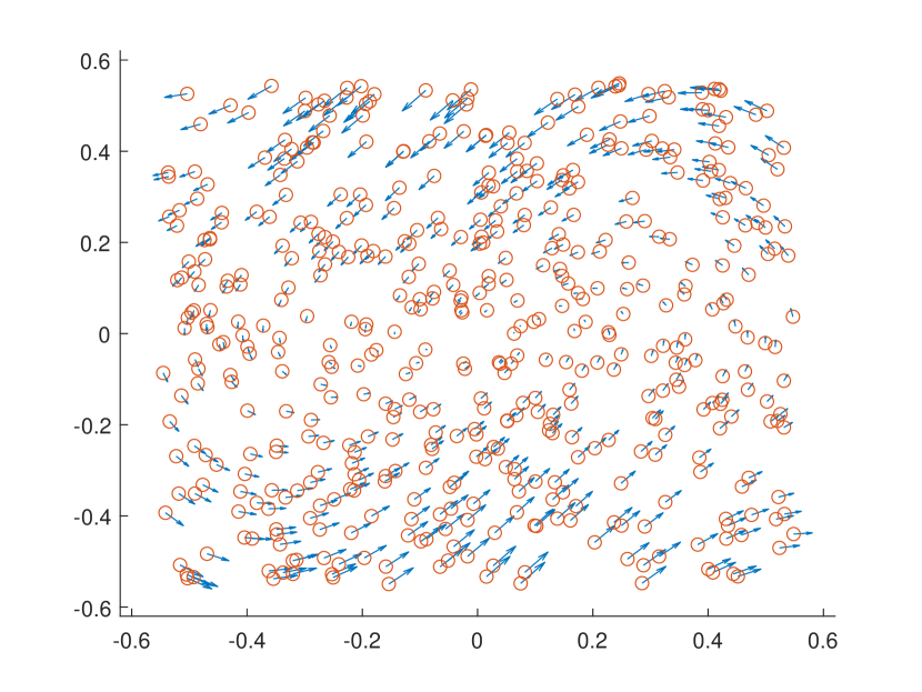
(a) The data used for the learning scheme.

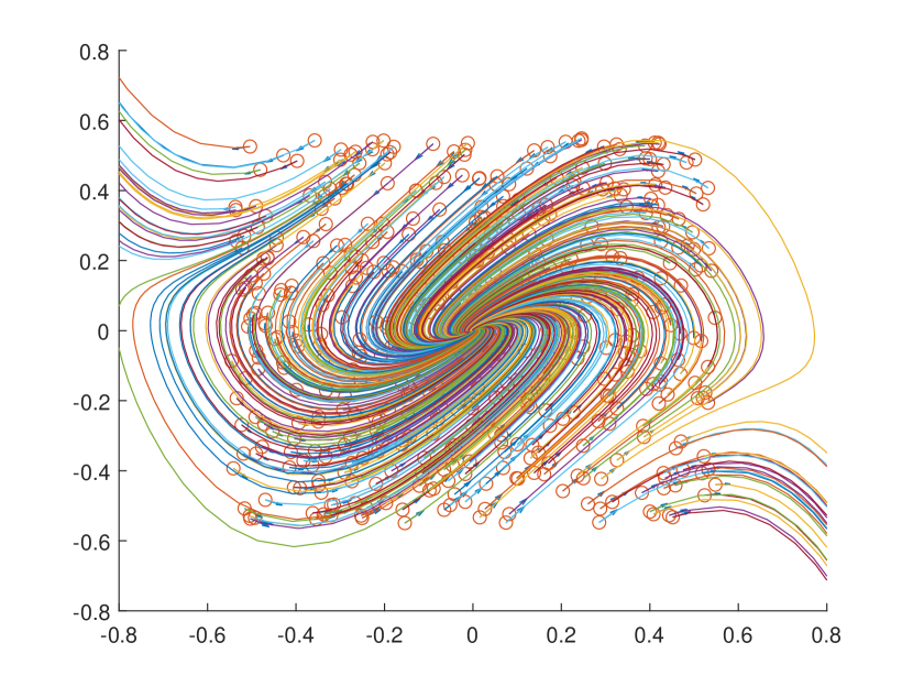
(b) Simulated trajectories (not used for learning).

Figure 6: The reverse time Van Del Pol oscillator.

We know an a-priori polytopic ROA $\mathcal{X}_{s}$, which is plotted in the center of Figure 7(b). A dataset with only 400 samples within $[-0.5,0.5]^{2}\subset\mathbb{R}^{2}$ is used to learn the underlying Lyapunov function: the positions $\{x_{i}\}$ and speeds $\{f(x_{i})\}$ of these samples are plotted in Figure 6(a). Similar to what we did in the last example, we simulate these data forward in Figure 6(b), while these trajectories are not used in the learning scheme. We can observe that both the lower right corner and the upper left corner in Figure 6(b) correspond to regions of unstable states. Even with only the access to the data in Figure 6(a), we can not give a clear idea about which region is safe, hence we apply Algorithm 3 to $[-0.5,0.5]^{2}$. In particular, the negativity tolerance $\epsilon$ is set to $10^{-3}$ and the tessellation is randomly generated by Delaunay triangulation [56]. The learnt Lyapunov function and its evaluation of $f(x)^{\top}\partial_{\rm Cl}L(x)$ on the learnt ROA are respectively plotted in Figure 7(a) and Figure 7(b). In particular, the maximal evaluation of $f(x)^{\top}\partial_{\rm Cl}L(x)$ on the learnt ROA is $-1.947\times 10^{-2}<0$.

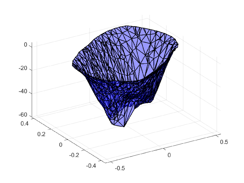
(a) Visualization of the Lyapunov function.

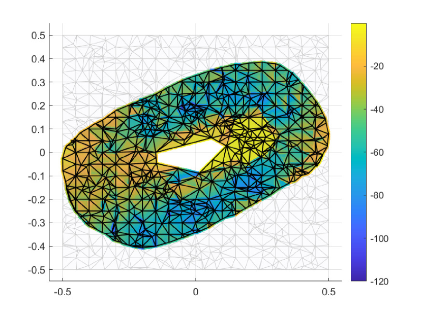
(b) Evaluation of $f(x)^{\top}\partial_{\rm Cl}L(x)$ on the learnt ROA.

Figure 7: The Lyapunov function learnt from a Van der Pol dataset.

7 Conclusion

Our results

In this work, we went all the way from proving a variant of stability theorem with non-smooth Lyapunov functions (LF), to actually implementing an algorithm for data-based region of attraction (RoA) estimation with unknown dynamic system. In the process, we went through proving a theorem for piecewise affine (PWA) LF computation and deriving a convex optimization program for computing such LF.

The originality of the method we propose is that it only requires a fixed dataset to compute an estimate of the RoA, from which it allows the user to deduce global information from local data and knowledge on the Lipschitz constant of the dynamic system. Hence, it can be used to study systems whose dynamic system cannot be easily sampled at will, through a relatively simple optimization problem that can be handled with interior point methods.

Future works

In this work, we proposed a learning scheme that can learn a robust Lyapunov function from a fixed dataset. However, with such minimal knowledge of the underlying dynamic system comes a big convex optimization even for a low-dimensional dynamic system. In future works, we plan on investigating how side information, particularly the RKHS structure [57], or other a-priori knowledge of the underlying dynamic system can be incorporated into the learning scheme, so that it can handle a higher-dimensional dynamic system.

References

- [1] A. M. Lyapunov, “The general problem of the stability of motion,” International journal of control, vol. 55, no. 3, pp. 531–534, 1992.
- [2] M. Hertneck, J. Köhler, S. Trimpe, and F. Allgöwer, “Learning an approximate model predictive controller with guarantees,” IEEE Control Systems Letters, vol. 2, no. 3, pp. 543–548, 2018.
- [3] S. Gao, S. Kong, and E. M. Clarke, “dreal: An smt solver for nonlinear theories over the reals,” in International conference on automated deduction, pp. 208–214, Springer, 2013.
- [4] Y.-C. Chang, N. Roohi, and S. Gao, “Neural lyapunov control,” Advances in neural information processing systems, vol. 32, 2019.
- [5] H. Dai, B. Landry, M. Pavone, and R. Tedrake, “Counter-example guided synthesis of neural network lyapunov functions for piecewise linear systems,” in 2020 59th IEEE Conference on Decision and Control (CDC), pp. 1274–1281, IEEE, 2020.
- [6] J. Kapinski, J. V. Deshmukh, S. Sankaranarayanan, and N. Aréchiga, “Simulation-guided lyapunov analysis for hybrid dynamical systems,” in Proceedings of the 17th international conference on Hybrid systems: computation and control, pp. 133–142, 2014.
- [7] S. Gao, J. Avigad, and E. M. Clarke, “-complete decision procedures for satisfiability over the reals,” in International Joint Conference on Automated Reasoning, pp. 286–300, Springer, 2012.
- [8] V. I. Zubov, Methods of AM Lyapunov and their application. P. Noordhoff, 1964.
- [9] P. Giesl, Construction of global Lyapunov functions using radial basis functions, vol. 1904. Springer, 2007.
- [10] P. A. Parrilo, Structured semidefinite programs and semialgebraic geometry methods in robustness and optimization. California Institute of Technology, 2000.
- [11] A. Oustry, M. Tacchi, and D. Henrion, “Inner approximations of the maximal positively invariant set for polynomial dynamical systems,” IEEE Control Systems Letters, vol. 3, no. 3, pp. 733–738, 2019.
- [12] D. Henrion and M. Korda, “Convex computation of the region of attraction of polynomial control systems,” IEEE Transactions on Automatic Control, vol. 59, no. 2, pp. 297–312, 2013.
- [13] M. Tacchi, C. Cardozo, D. Henrion, and J. B. Lasserre, “Approximating regions of attraction of a sparse polynomial differential system,” IFAC-PapersOnLine, vol. 53, no. 2, pp. 3266–3271, 2020.
- [14] A. A. Ahmadi and A. Majumdar, “Dsos and sdsos optimization: more tractable alternatives to sum of squares and semidefinite optimization,” SIAM Journal on Applied Algebra and Geometry, vol. 3, no. 2, pp. 193–230, 2019.
- [15] Z. Sun, “Stability of piecewise linear systems revisited,” Annual Reviews in Control, vol. 34, no. 2, pp. 221–231, 2010.
- [16] H. Lin and P. J. Antsaklis, “Stability and stabilizability of switched linear systems: a survey of recent results,” IEEE Transactions on Automatic control, vol. 54, no. 2, pp. 308–322, 2009.
- [17] A. Alessio and A. Bemporad, “A survey on explicit model predictive control,” in Nonlinear model predictive control, pp. 345–369, Springer, 2009.
- [18] M. Johansson and A. Rantzer, “Computation of piecewise quadratic lyapunov functions for hybrid systems,” in 1997 European Control Conference (ECC), pp. 2005–2010, IEEE, 1997.
- [19] H. Ravanbakhsh and S. Sankaranarayanan, “Learning control lyapunov functions from counterexamples and demonstrations,” Autonomous Robots, vol. 43, no. 2, pp. 275–307, 2019.
- [20] R. Schwan, C. N. Jones, and D. Kuhn, “Stability verification of neural network controllers using mixed-integer programming,” arXiv preprint arXiv:2206.13374, 2022.
- [21] A. Solar-Lezama, L. Tancau, R. Bodik, S. Seshia, and V. Saraswat, “Combinatorial sketching for finite programs,” in Proceedings of the 12th international conference on Architectural support for programming languages and operating systems, pp. 404–415, 2006.
- [22] A. Solar-Lezama, Program synthesis by sketching. University of California, Berkeley, 2008.
- [23] S. Chen, M. Fazlyab, M. Morari, G. J. Pappas, and V. M. Preciado, “Learning lyapunov functions for hybrid systems,” in Proceedings of the 24th International Conference on Hybrid Systems: Computation and Control, pp. 1–11, 2021.
- [24] A. Abate, D. Ahmed, M. Giacobbe, and A. Peruffo, “Formal synthesis of lyapunov neural networks,” IEEE Control Systems Letters, vol. 5, no. 3, pp. 773–778, 2020.
- [25] T. A. Johansen, “Computation of lyapunov functions for smooth nonlinear systems using convex optimization,” Automatica, vol. 36, no. 11, pp. 1617–1626, 2000.
- [26] P. Giesl, B. Hamzi, M. Rasmussen, and K. N. Webster, “Approximation of lyapunov functions from noisy data,” arXiv preprint arXiv:1601.01568, 2016.
- [27] S. F. Marinósson, “Lyapunov function construction for ordinary differential equations with linear programming,” Dynamical Systems: An International Journal, vol. 17, no. 2, pp. 137–150, 2002.
- [28] P. M. Julian, A high-level canonical piecewise linear representation: Theory and applications. PhD thesis, Universidad Nacional del Sur (Argentina), 1999.
- [29] R. Baier, L. Grüne, and S. F. Hafstein, “Linear programming based lyapunov function computation for differential inclusions,” Discrete & Continuous Dynamical Systems-B, vol. 17, no. 1, p. 33, 2012.
- [30] S. F. Hafstein, “An algorithm for constructing lyapunov functions.,” Electronic Journal of Differential Equations, vol. 2007, 2007.
- [31] R. T. Rockafellar and R. J.-B. Wets, Variational analysis, vol. 317. Springer Science & Business Media, 2009.
- [32] J.-B. Hiriart-Urruty and C. Lemaréchal, Fundamentals of convex analysis. Springer Science & Business Media, 2004.
- [33] F. H. Clarke, Optimization and Nonsmooth Analysis. Classics in Applied Mathematics, SIAM, 1990.
- [34] J. P. La Salle, The stability of dynamical systems. SIAM, 1976.
- [35] M. Della Rossa, Non-Smooth Lyapunov Functions for Stability Analysis of Hybrid Systems. PhD thesis, Institut National des Sciences Appliquées de Toulouse, 2020.
- [36] H. L. Royden and P. Fitzpatrick, Real analysis, vol. 32. Macmillan New York, 1988.
- [37] F. Aurenhammer, “A criterion for the affine equivalence of cell complexes in r d and convex polyhedra in r d+ 1,” Discrete & Computational Geometry, vol. 2, no. 1, pp. 49–64, 1987.
- [38] S. Boyd, S. P. Boyd, and L. Vandenberghe, Convex optimization. Cambridge university press, 2004.
- [39] A. Ben-Tal and A. Nemirovski, “Robust optimization–methodology and applications,” Mathematical programming, vol. 92, no. 3, pp. 453–480, 2002.
- [40] J.-P. Calliess, S. J. Roberts, C. E. Rasmussen, and J. Maciejowski, “Lazily adapted constant kinky inference for nonparametric regression and model-reference adaptive control,” Automatica, vol. 122, p. 109216, 2020.
- [41] S. Saitoh and Y. Sawano, Theory of reproducing kernels and applications. Springer, 2016.
- [42] C. K. Williams and C. E. Rasmussen, Gaussian processes for machine learning, vol. 2. MIT press Cambridge, MA, 2006.
- [43] P. Scharnhorst, E. T. Maddalena, Y. Jiang, and C. N. Jones, “Robust uncertainty bounds in reproducing kernel hilbert spaces: A convex optimization approach,” arXiv preprint arXiv:2104.09582, 2021.
- [44] L. Sabug Jr, F. Ruiz, and L. Fagiano, “Smgo: A set membership approach to data-driven global optimization,” Automatica, vol. 133, p. 109890, 2021.
- [45] M. Canale, L. Fagiano, and M. Milanese, “Set membership approximation theory for fast implementation of model predictive control laws,” Automatica, vol. 45, no. 1, pp. 45–54, 2009.
- [46] Y. Nesterov and A. Nemirovskii, Interior-point polynomial algorithms in convex programming. SIAM, 1994.
- [47] S. F. Hafstein*, “A constructive converse lyapunov theorem on asymptotic stability for nonlinear autonomous ordinary differential equations,” Dynamical Systems, vol. 20, no. 3, pp. 281–299, 2005.
- [48] P. Giesl and S. Hafstein, “Review on computational methods for lyapunov functions,” Discrete & Continuous Dynamical Systems-B, vol. 20, no. 8, p. 2291, 2015.
- [49] A. Subbaraman and A. R. Teel, “A matrosov theorem for strong global recurrence,” Automatica, vol. 49, no. 11, pp. 3390–3395, 2013.
- [50] S. P. Meyn and R. L. Tweedie, Markov chains and stochastic stability. Springer Science & Business Media, 2012.
- [51] H. Krieg, Modeling and solution of continuous set covering problems by means of semi-infinite optimization. Fraunhofer Verlag, 2019.
- [52] E. D. Andersen, C. Roos, and T. Terlaky, “On implementing a primal-dual interior-point method for conic quadratic optimization,” Mathematical Programming, vol. 95, no. 2, pp. 249–277, 2003.
- [53] L. Vandenberghe and M. S. Andersen, “Chordal graphs and semidefinite optimization,” Foundations and Trends in Optimization, vol. 1, no. 4, pp. 241–433, 2015.
- [54] K. Rybnikov, Polyhedral partitions and stresses. Queen’s University at Kingston, 2000.
- [55] F. Aurenhammer, “Power diagrams: properties, algorithms and applications,” SIAM Journal on Computing, vol. 16, no. 1, pp. 78–96, 1987.
- [56] B. Delaunay et al., “Sur la sphere vide,” Izv. Akad. Nauk SSSR, Otdelenie Matematicheskii i Estestvennyka Nauk, vol. 7, no. 793-800, pp. 1–2, 1934.
- [57] P.-C. Aubin-Frankowski and Z. Szabó, “Hard shape-constrained kernel machines,” Advances in Neural Information Processing Systems, vol. 33, pp. 384–395, 2020.