Non-Linearity-Free prediction of the growth-rate $f\sigma_{8}$ using Convolutional Neural Networks

Abstract

The growth-rate $f\sigma_{8}(z)$ of the large-scale structure of the Universe is an important dynamic probe of gravity that can be used to test for deviations from General Relativity. However, in order for galaxy surveys to extract this key quantity from cosmological observations, two important assumptions have to be made: i) a fiducial cosmological model, typically taken to be the cosmological constant and cold dark matter ($\Lambda$CDM) model and ii) the modeling of the observed power spectrum from H$\alpha$ emitters, especially at non-linear scales, which is particularly dangerous as most models used in the literature are phenomenological at best. In this work, we propose a novel approach involving convolutional neural networks (CNNs), trained on the Quijote N-body simulations, to predict $f\sigma_{8}(z)$ directly and without assuming a model for the non-linear part of the power spectrum, thus avoiding the second of the aforementioned assumptions. We find that the predictions for the value of $f\sigma_{8}$ from the CNN are in excellent agreement with the fiducial values, while the errors are within a factor of order unity from those of the traditionally optimistic Fisher matrix approach, assuming an ideal fiducial survey matching the specifications of the Quijote simulations. Thus, we find the CNN reconstructions provide a viable alternative in order to avoid the theoretical modeling of the non-linearities at small scales when extracting the growth-rate.

1 Introduction

Recent cosmological observations indicate that the Universe is experiencing a phase of accelerated expansion, which is typically attributed to a new form of matter, i.e., dark energy, that is responsible for this phenomenon. Within the context of the Friedmann-Lemaître-Robertson-Walker (FLRW) cosmology, this new dark energy component is frequently attributed to the cosmological constant $\Lambda$, which is introduced regardless of the fine-tuning issues that this may cause [1, 2]. Together with the assumption of a cold dark matter (CDM) component, these two ingredients make up the so-called $\Lambda$CDM model, which is currently the concordance cosmological model [3].

The large-scale structure (LSS) of the Universe encodes very important details that are crucial to test cosmological models, as it provides information about the late-time evolution of the Universe and the structure of the matter density field. Both are useful for constraining the current values of the fractional density parameters for CDM, baryonic matter, and dark energy: $\Omega_{\mathrm{m,0}}$, $\Omega_{\mathrm{b,0}}$ and $\Omega_{\mathrm{\Lambda,0}}$ respectively, and many other parameters like the clustering strength $\sigma_{8}$ [4, 5]. They are also important probes to search for possible deviations from general relativity.

An overriding challenge in modern cosmology is understanding the features of dark energy, and here lies the importance of obtaining highly accurate data from forthcoming cosmological missions such as Euclid [6], LSST [7], and DESI [8], which aim to provide percent measurements of the various key parameters related to the LSS. In order to make sense of the plethora of currently available cosmological models and observations [9, 10], it is necessary to develop valuable statistical tools. In particular, Machine Learning (ML) has attracted increasing attention as it simplifies the usually computationally expensive procedures for data treatment [11]. Simulations also play an indispensable role in understanding the whole picture of the LSS, since some information is particularly difficult to extract due to the non-linearity nature of the system. This is the motivation behind the Quijote N-body simulations, consisting of CDM particle simulations that allow quantifying data on the matter field in the fully non-linear regime and with different statistics [12].

One way of probing the dynamics of LSS is by measuring the growth of matter density perturbations $\delta_{m}=\delta\rho_{m}/\rho_{m}$, where $\rho_{m}$ is the background matter density and $\delta\rho_{m}$ its linear order perturbation, and its growth rate that is usually represented by its logarithmic derivative $f=\frac{d\ln\delta_{m}}{d\ln a}$. However, when dealing with galaxy surveys, the observed quantity is, in fact, the galaxy density $\delta_{g}$, which is connected to the matter perturbations through a bias parameter that changes from survey to survey: $\delta_{g}=b\,\delta_{m}$ and depending on the type of galaxy observed [13]. At some redshift bin $z_{i}$, the growth rate $f(z_{i})$ can be combined with the bias $b(z_{i})$ to give rise to the so-called velocity-density coupling parameter $\beta(z_{i})=f(z_{i})/b(z_{i})$, while the combination of $b(z_{i})\sigma_{8}(z_{i})$ can also be independently measured [14], where $\sigma_{8}(z)$ is the root mean square (RMS) density fluctuation in a sphere of radius $R=8\mathrm{Mpc}/h$. Therefore the combination $f\sigma_{8}(z)\equiv f(z)\sigma(z)$ is independent of bias and can be measured via redshift-space distortions [15].

However, this approach has the issue that in order to extract the $f\sigma_{8}(z)$ quantity, two main assumptions have to be made: first, that of a cosmological model (typically assumed to be the $\Lambda$CDM model), as we need to convert the redshifts of galaxies and coordinates in the sky to distances in order to extract the correlation function [16]. Second, we need to assume a model for the non-linear part of the power spectrum (at scales $k\gtrsim 0.3\,h/\mathrm{Mpc}$), typically done with phenomenological models [17, 18, 19, 20, 21].

This approach has also led to the creation of several $f\sigma_{8}(z)$ data set compilations, see for example, Refs. [14, 22, 23] and references therein, where the data have an explicit dependence on the cosmology used. Even though this can be somewhat easily corrected for via an Alcock-Paczynski (AP) type correction [22], the second issue of the model dependence on the non-linear power spectrum is more insidious as all models used are phenomenological, and thus far, there is no way to correct for that a posteriori.

One approach which has been recently proposed to extract cosmological parameters in a theory-agnostic manner is via ML and, in particular, by training Convolutional Neural Networks (CNNs) on N-body simulations and then extracting the parameters from the LSS statistics [24]. This approach was also further expanded to also extract the cosmological density and velocity fields from N-body simulations [25, 26]. These ML approaches have the main advantages that after the original training has occurred, any subsequent evaluations are practically instantaneous, and more importantly, they allow for extracting the quantities of interest with minimal assumptions.

In this work, we aim to extract and compare the growth-rate $f\sigma_{8}$ quantity by leveraging ML techniques, in particular by training a CNN directly on N-body simulations at different redshift bins and also on the power spectrum of these simulations. For comparison, we also calculated the estimated errors of $f\sigma_{8}$ for an ideal survey corresponding to our simulations. Thus, while we do not avoid the cosmological model dependence, we avoid the assumption of the modeling of the non-linear power spectrum.

The layout of our paper is as follows: in Sec. 2, we briefly summarize the theoretical background of our analysis, while in Sec. 3, we present the details for the Quijote simulations used in our analysis. Then in Sec. 4, we describe the results of our ML analysis using the density field of the simulations, while in Sec. 5, we compare our results to the conventional likelihood inference. Finally, in Sec. 6, we summarize our conclusions.

2 Theoretical framework

2.1 The $\Lambda$CDM model and the growth-rate

In this work, we will consider general relativity and a flat $\Lambda$CDM universe with an equation of state of $w=-1$ for dark energy.

At the background level, the Hubble parameter in a flat $\Lambda$CDM model is given by the first Friedmann equation as usual:

$$H(a)^{2}=H_{0}^{2}\,\left(\Omega_{m,0}a^{-3}+1-\Omega_{m,0}\right),$$ (2.1)

where $H_{0}$ is the Hubble constant and the matter density $\Omega_{m,0}$ can be related to the scale factor $a$ by:

$$\Omega_{m}(a)=\frac{\Omega_{m,0}a^{-3}}{{H(a)^{2}}/{H_{0}^{2}}}.$$ (2.2)

Also, assuming a flat universe we can calculate the comoving distance $D(z)$ from us to a redshift $z$ as

$$D(z)=\int^{z}_{0}\frac{c\ dz^{\prime}}{H(z^{\prime})},$$ (2.3)

where $c$ is the speed of light and $H(z)$ is Hubble parameter at redshift $z$ calculated via Eq. (2.1), when neglecting radiation and neutrinos at late times.

On the other hand, observations from the LSS and the cosmic microwave background (CMB) also suggest the existence of small $\sim\mathcal{O}(10^{-5})$ perturbations. Thus, we have to work in the framework of a perturbed FLRW metric as the gravitational instability produced by density fluctuations plays a crucial role in seeding the structures at large scales. In the conformal Newtonian gauge, we consider scalar metric perturbations $\Psi$ and $\Phi$, so the perturbed metric can be written as [27, 28]

$$ds^{2}=a(\tau)^{2}\left[-(1+2\Psi(\vec{x},\tau))d\tau^{2}+(1-2\Phi(\vec{x},\tau))d\vec{x}^{2}\right],$$ (2.4)

where the potentials depend on the space-time point $x^{\mu}=(\vec{x},\tau)$, with $\tau$ being the conformal time, while the scale factor $a(\tau)$ only depends on the conformal time.

In general, we can assume that the matter component behaves as a perfect fluid and described by the stress-energy tensor:

$$T_{\nu}^{\mu}=P\delta_{\nu}^{\mu}+(\rho+P)U^{\mu}U_{\nu},$$ (2.5)

where the 4-velocity is $U^{\mu}=\frac{dx^{\mu}}{\sqrt{-ds^{2}}}$, the total density is $\rho=\bar{\rho}+\delta\rho$, the total pressure is $P=\bar{P}+\delta P$, $\bar{\rho}=\bar{\rho}(\tau)$ and $\delta\rho=\delta\rho(\vec{x},\tau)$ and $\delta P=\delta P(\vec{x},\tau)$ are the density and pressure perturbations respectively, while $\bar{P}=\bar{P}(\tau)$ are the background energy density and pressure quantities. Therefore, the stress-energy tensor components are [29]:

$$T_{0}^{0} = -(\bar{\rho}+\delta\rho),$$ (2.6)

$$T_{i}^{0} = (\bar{\rho}+\bar{P})u_{i},$$ (2.7)

$$T_{j}^{i} = (\bar{P}+\delta P)\delta_{j}^{i}+\Sigma_{j}^{i},$$ (2.8)

where $\Sigma_{j}^{i}\equiv T_{j}^{i}-\delta_{j}^{i}\,T_{k}^{k}/3$ is the anisotropic stress and $u=\dot{\vec{x}}$. The dot denotes derivative with respect to $\tau$ [30]. Recall that the energy-momentum tensor follows the conservation law $T^{\mu\nu}{}_{;\nu}=0$, as a consequence of the Bianchi identities [29].

To study the evolution of the perturbed variables, we resort to the perturbed Einstein equations in $k$-space [27, 29]:

$$k^{2}\Phi+3\frac{\dot{a}}{a}\left(\dot{\Phi}+\frac{\dot{a}}{a}\Psi\right) = 4\pi G_{\mathrm{N}}a^{2}\delta T_{0}^{0},$$ (2.9)

$$k^{2}\left(\dot{\Phi}+\frac{\dot{a}}{a}\Psi\right) = 4\pi G_{\mathrm{N}}a^{2}(\bar{\rho}+\bar{P})\theta,$$ (2.10)

$$\ddot{\Phi}+\frac{\dot{a}}{a}(\dot{\Psi}+2\dot{\Phi})+\left(2\frac{\ddot{a}}{a}-\frac{\dot{a}^{2}}{a^{2}}\right)\Psi+\frac{k^{2}}{3}(\Phi-\Psi) = \frac{4\pi}{3}G_{\mathrm{N}}a^{2}\delta T_{i}^{i},$$ (2.11)

$$k^{2}(\Phi-\Psi) = 12\pi G_{\mathrm{N}}a^{2}(\bar{\rho}+\bar{P})\sigma,$$ (2.12)

where the fluid velocity is defined via $\theta=ik_{j}u^{j}$ and $k_{j}$ is the wavenumber of the perturbations in Fourier space. We can also rewrite the anisotropic stress as $(\bar{\rho}+\bar{P})\sigma\equiv-(-\hat{k}_{i}\hat{k}_{j}-\frac{1}{3}\delta_{ij})\Sigma^{ij}$.

By taking the following approximations: sub-horizon (only the modes in the Hubble radius are important) and quasi-static (neglect terms with time derivatives), we can simplify the perturbed Einstein equations. Let us consider the perturbation of the Ricci scalar, and see how it simplifies with these approximations:

$$\delta R =-\frac{12\left(\mathcal{H}^{2}+\dot{\mathcal{H}}\right)}{a^{2}}\Psi-\frac{4k^{2}}{a^{2}}\Phi+\frac{2k^{2}}{a^{2}}\Psi-\frac{18\mathcal{H}}{a^{2}}\dot{\Phi}-\frac{6\mathcal{H}}{a^{2}}\dot{\Psi}-\frac{6\ddot{\Phi}}{a^{2}},$$ (2.13)

$$\simeq-\frac{4k^{2}}{a^{2}}\Phi+\frac{2k^{2}}{a^{2}}\Psi,$$

then, we can find the following expressions for the Newtonian potentials, see [29]:

$$\Psi(k,a)=-4\pi G_{\mathrm{N}}\frac{a^{2}}{k^{2}}\mu(k,a)\bar{\rho}_{\mathrm{m}}\delta_{\mathrm{m}},$$ (2.14)

$$\Phi(k,a)=-4\pi G_{\mathrm{N}}\frac{a^{2}}{k^{2}}Q_{\mathrm{eff}}(k,a)\bar{\rho}_{\mathrm{m}}\delta_{\mathrm{m}},$$ (2.15)

where $\mu(k,a)\equiv G_{\mathrm{eff}}(k,a)/G_{\mathrm{N}}$ is used to denote an evolving Newton’s constant. In GR the two parameters $\mu(k,a)$ and $Q_{\mathrm{eff}}(k,a)$ can be shown to be equal to unity, but in modified gravity theories they are, in general, time and scale dependent [29].

From the context developed before and by using the continuity equations that come from the conservation of the energy-momentum tensor (via the Bianchi identities), we arrive to a second-order differential equation that describes the evolution of the matter density perturbations (in the absence of massive neutrinos), which is valid in the context of most modified gravity models [31]:

$$\delta^{\prime\prime}_{\mathrm{m}}(a)+\left(\frac{3}{a}+\frac{H^{\prime}(a)}{H(a)}\right)\delta^{\prime}_{\mathrm{m}}(a)-\frac{3\Omega_{\mathrm{m,0}}\,\mu(k,a)}{2a^{5}\,H(a)^{2}/H_{0}^{2}}\delta_{\mathrm{m}}(a)=0,$$ (2.16)

for which we assume the initial conditions $\delta_{\mathrm{m}}(a\ll 1)\sim a$ and $\delta^{\prime}_{\mathrm{m}}(a\ll 1)\sim 1$ at some initial time in the matter domination era, e.g. $a=10^{-3}$.

In GR and the $\Lambda$CDM model ($\mu=1$), the analytical solution for the growing mode can be found by directly solving Eq. (2.16) and is given by [32, 33, 34, 35]

$$\delta_{\mathrm{m}}(a)=a\cdot{}_{2}F_{1}\left(\frac{1}{3},1;\frac{11}{6};a^{3}\left(1-\frac{1}{\Omega_{\mathrm{m,0}}}\right)\right),$$ (2.17)

where we use the quasi-static and sub-horizon approximations [31] and ${}_{2}F_{1}$ is the Gauss hypergeometric function expressed as

$${}_{2}F_{1}(a,b,c,z)=\sum^{\infty}_{n=0}\frac{(a)_{n}(b)_{n}}{(c)_{n}}\frac{z^{n}}{n!},$$ (2.18)

where $(x)_{n}$ is the rising factorial calculated as

$$(x)_{n}=x(x+1)(x+2)\cdots(x+n-1).$$ (2.19)

With this in mind, we can define several key quantities: the growth rate $f$, and $\sigma_{8}$, which is the root mean square (RMS) normalization of the matter power spectrum as:

$$f(a) =\frac{\mathrm{d}\log\delta_{\mathrm{m}}}{\mathrm{~{}d}\log a},$$ (2.20)

$$\sigma_{8}(a) =\sigma_{8,0}\frac{\delta_{\mathrm{m}}(a)}{\delta_{\mathrm{m}}(1)},$$ (2.21)

$$\sigma_{8,0}^{2} =\left\langle\delta_{\mathrm{m}}(x)^{2}\right\rangle.$$ (2.22)

It’s important to mention that in general, we have to correct the data for the Alcock-Paczynski effect (as different surveys use different fiducial cosmologies) [36, 37, 38]. The combination of the growth rate $f(z)$ and $\sigma_{8}(z)$ gives rise to a new bias-independent variable $f\sigma_{8}$, that is in fact what is measured by galaxy surveys from redshift space distortions (RSDs):

$$f\sigma_{8}(a)=a\frac{\delta_{\mathrm{m}}^{\prime}(a)}{\delta_{\mathrm{m}}(1)}\cdot\sigma_{8,0}.$$ (2.23)

This quantity can be directly measured from current and forthcoming galaxy surveys and several compilations exist in the literature [14, 22, 23]. Thus, if a growth rate measurement has been obtained via a fiducial cosmology $H^{\prime}(z)$, then the corresponding $f\sigma_{8}$ value is obtained for the true cosmology $H(z)$ via an AP-like correction [39, 22, 38]:

$$f\sigma_{8}(z)\simeq\frac{H(z)D_{A}(z)}{H^{\prime}(z)D_{A}^{\prime}(z)}\,f\sigma_{8}^{\prime}(z).$$ (2.24)

Nonetheless, one of the main advantages of the $f\sigma_{8}$ growth-rate is that it is a direct dynamic probe of gravity since, as can be seen from Eq. (2.16), the dependence on the gravitational theory appears explicitly via the normalized evolving Newton’s constant $\mu(k,a)$ and indirectly via the Hubble parameter $H(a)$. On the other hand, one of its main weaknesses is also that the measurements, as currently made by the galaxy surveys, suffer from model dependence (typically assumed to be the $\Lambda$CDM model) and by the fact that the modeling of the non-linear scales is phenomenological [17, 18, 19, 20, 21].

2.2 Error estimates from the Fisher matrix

Here we now briefly summarize the so-called Fisher matrix approach that can be used to forecast the measurement errors for cosmological observables from forthcoming galaxy surveys [40, 41, 42, 21]. This approach allows us to obtain a typically optimistic estimate of the errors, assuming some particular specifications for a survey in question.

The first step is to assume a fiducial galaxy survey that is split in $N_{\mathrm{bins}}$ redshift bins, then the Fisher matrix in every bin $i$ is [40, 41, 42, 21]

$$F_{\alpha\beta}^{\mathrm{bin}}(z_{i})=\frac{1}{8\pi^{2}}\int_{-1}^{1}d\mu\int_{k_{\mathrm{min}}}^{k_{\mathrm{max}}}k^{2}\,dk\,\bigg{[}\frac{\partial\ln P_{\mathrm{obs}}}{\partial\theta_{\alpha}}\frac{\partial\ln P_{\mathrm{obs}}}{\partial\theta_{\beta}}\bigg{]}\,V_{\mathrm{eff}}(z_{i},k,\mu),$$ (2.25)

where $k$ is the Fourier wavenumber, $\mu$ is the cosine of the angle between the line-of-sight and the wave-vector $\mathbf{k}$, $\theta_{\alpha}$ is the set of parameters varied in the Fisher matrix (to be specified below) and

$$V_{\mathrm{eff}}(k,\mu;z)=V_{s}(z)\,\Big{[}\frac{n(z)\,P_{\mathrm{obs}}(k,\mu;z)}{n(z)\,P_{\mathrm{obs}}(k,\mu;z)+1}\Big{]}^{2},$$ (2.26)

is the effective volume of the survey, where $V_{s}(z)$ is the comoving volume of a region covering a solid angle between the redshift limits of the bin. The integral over the wave-numbers $k$ in Eq. (2.25) is done up to a maximum value $k_{\mathrm{max}}$, chosen such that we remain within approximately linear scales $k_{\mathrm{max}}=0.25\,h\,\mathrm{Mpc}^{-1}$ (our pessimistic scenario) or going slightly into the non-linear regime $k_{\mathrm{max}}=0.30\,h\,\mathrm{Mpc}^{-1}$ (our optimistic scenario). In what follows, we mainly focus on the pessimistic scenario.

Finally, the observed power spectrum is

$$P_{\mathrm{obs}}(k,\mu;z)=\frac{1}{q^{2}_{\perp}\,q_{\parallel}}\,{\frac{\big{[}b\sigma_{8}(z)+f\sigma_{8}(z)\mu^{2}\big{]}^{2}}{1+[f(z)k\mu\sigma_{\mathrm{p}}]^{2}}}\,\frac{P_{\mathrm{dw}}(k,\mu;z)}{\sigma_{8}^{2}(z)}F_{z}(k,\mu;z)+P_{s}(z),$$ (2.27)

where $q_{\perp}$, $q_{\parallel}$ are the AP projection coefficients, $b$ is the bias, $\sigma_{\mathrm{p}}$ is a non-linear parameter computed from the linear power spectrum, $P_{\mathrm{dw}}$ is the “de-wiggled” power spectrum, $F_{z}$ accounts for the smearing of the galaxy density field along the line of sight direction and finally, $P_{s}(z)$ is a scale-independent offset due to imperfect removal of shot noise (see Ref. [42] for more details). In this work we calculate the power spectrum numerically, using the Boltzmann code CLASS [43, 44].

With these in mind, in order to actually calculate the Fisher matrix we need to evaluate the derivatives of the observed power spectrum. Unfortunately, this can only be done numerically, thus we employ a two-point central difference formula for the derivatives. We also need to de-wiggle the power spectrum, and to do this we apply a Savitzky-Golay filter with a window size of 201 and polynomial order equal to 3.

Of crucial importance is also the choice of the bias function $b(z)$, as this appears in the $b\sigma_{8}(z)$ quantity. Here we choose to model the halo bias as

$$b_{\mathrm{halo}}(z)=A+B\,e^{C\,z},$$ (2.28)

where $A=0.648$, $B=0.689$ and $C=0.792$ are free parameters determined by fitting the model to the halo catalog. Then, the total Fisher matrix is obtained by summing over all the redshift bins as:

$$F_{\alpha\beta}=\sum_{i=1}^{N_{\mathrm{bins}}}F_{\alpha\beta}^{\mathrm{bin}}(z_{i}).$$ (2.29)

Finally, we should note that compared to other analyses, e.g. that of Refs. [42, 21], we choose to vary for the Fisher matrix only the cosmological parameters, namely the parameter set $\theta_{\mathrm{cosmo}}=\{\Omega_{\mathrm{b,0}},\Omega_{\mathrm{m,0}},h,n_{s},\ln\left(10^{10}A_{s}\right),\sum m_{\nu}\}$, along with the set of non-cosmological $\theta_{\mathrm{non-cosmo}}=\{\sigma_{p},P_{s}\}$, which are related to the non-linear prescription and the shot noise (see Ref. [21] for more info). Unlike other analyses, we do not vary with respect to quantities in each bin, such as the angular diameter distance $D_{A}(z_{i})$, the Hubble parameter $H(z_{i})$, the growth rate $f\sigma_{8}(z_{i})$ or $b\sigma_{8}(z_{i})$, as all of them already in principle depend on the vector of cosmological parameters $\theta_{\mathrm{cosmo}}$. Clearly, by including the aforementioned quantities as free parameters we would be double-counting the information, as we have already fixed our fiducial model to be the $\Lambda$CDM model. Thus, our final vector of parameters for the Fisher matrix is $\theta_{\mathrm{total}}=\theta_{\mathrm{cosmo}}+\theta_{\mathrm{non-cosmo}}$. We also assume that all parameters in our analysis are constant across all the redshift bins.

Then, after the total Fisher matrix has been determined, we perform an error-propagation to go from the covariance matrix $C_{\alpha\beta}\equiv F^{-1}_{\alpha\beta}$ of the $\theta_{\mathrm{total}}$ parameters to the covariance matrix of the growth rate values $f\sigma_{8}(z_{i})$ in each redshift bin. This is done in practice via:

$$C_{ij}=\frac{\partial f\sigma_{8,i}}{\partial\theta_{\alpha}}\,\frac{\partial f\sigma_{8,j}}{\partial\theta_{\beta}}\,C_{\alpha\beta},$$ (2.30)

where we calculate the transformation matrix $J^{i}_{\alpha}\equiv\frac{\partial f\sigma_{8,i}}{\partial\theta_{\alpha}}$ numerically as well. Then, the errors of $f\sigma_{8}(z_{i})$ in each redshift bin are simply given by the diagonal elements of the covariance matrix as

$$\sigma_{f\sigma_{8}(z_{bin,i})}^{2}=C_{ii}.$$ (2.31)

We have made extensive comparisons with other analyses, e.g. that of Refs. [42, 21], and we find that the results of our approach are in excellent agreement, thus we are confident in the robustness of our methodology.

3 The Quijote simulations

The Quijote simulations, see Ref. [12], are a set of 44100 N-body simulations created via the TreePM code Gadget-III in boxes of sides of 1 Gpc/h, where $h$ is the reduced Hubble constant. In this work, we use these simulations to train and test of our CNN.

The Quijote simulations have $2,000$ realizations which vary the value of cosmological parameters $(\Omega_{m},\Omega_{b},h,n_{s},\sigma_{8})$, chosen by the Latin-hypercube, and whose limits are set by

$$\Omega_{m} \in [0.1,0.5],$$

$$\Omega_{b} \in [0.03,0.07],$$

$$h \in [0.5,0.9],$$

$$n_{s} \in [0.8,1.2],$$

$$\sigma_{8} \in [0.6,1.0].$$ (3.1)

Each simulation box has $512^{3}$ dark matter particles and each realization has $5$ snapshots at redshifts $z=[3.0,\ 2.0,\ 1.0,\ 0.5,\ 0.0]$. In Fig. 1, we show the distribution of $f\sigma_{8}$ for the realizations of the simulation and for each redshift.

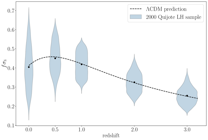
Figure 1: The distribution of the $f\sigma_{8}$ parameter values for Latin-hypercube realizations of the Quijote simulations at their corresponding redshifts. Black dots represent the mean value at each redshift and the dashed curve shows the $\Lambda$CDM prediction.

3.1 The halo catalog

$z$ range	$z$ mean	relative number	$n_{\rm halo}$	comoving distance	box size
			$[(h^{-1}\mathrm{Gpc})^{-3}]$	[$h^{-1}\mathrm{Mpc}$]	[$\mathrm{deg}$]
$[0.5,1.0]$	0.75	2	$8.0\times 10^{3}$	$1.9\times 10^{3}$	$30.2$
$[1.0,1.5]$	1.25	4	$1.6\times 10^{4}$	$2.7\times 10^{3}$	$20.9$
$[1.5,2.0]$	1.75	3	$1.2\times 10^{4}$	$3.4\times 10^{3}$	$16.9$
$[2.0,3.0]$	2.5	1	$8.0\times 10^{3}$	$4.1\times 10^{3}$	$14.0$

Table 1: Specifications for the mock simulation. The relative number is the expected number of halos given our assumed toy observation, which roughly corresponds to the Euclid survey, and $n_{\rm halo}$ is the number of halos included in the simulation box after the random draw. We also provide observation-related quantities, the comoving distance to the mean redshift and subtended angle of the simulation box placed at the comoving distance.

The Quijote simulations have a halo catalog identified by a Friends-Of-Friends (FOF) algorithm, in which each halo has at least $20$ dark matter particles. Therefore, the lower limit of the halo mass is $\mathcal{O}(10^{12})$ - $\mathcal{O}(10^{13})\ [M_{\odot}/h]$ (the value varies with the values of the cosmological parameters).

As a rough approximation, we probe redshifts from 0.5 to 3 spanned in 4 redshift bins, where mean redshifts are $z=[0.75,1.25,1.75,2.5]$ for the analysis of the halo distribution. And then, we assume the redshift halo distribution, that roughly corresponds to the Euclid survey, and randomly pick up halos such that the redshift distribution matches to the relative numbers in Table. 1. In this table, the mean of the comoving number density of the halos in each redshift bin over 2,000 realizations after the picking up is also shown. We also provide a relation between the box size ($=1\ \mathrm{Gpc}/h$) for each redshift. We can calculate the apparent angular size of the object whose physical size $l$ at redshift $z$ as

$$\theta\ [\mathrm{rad}]=2\arctan{\left(\frac{l/a}{2D(z)}\right)},$$ (3.2)

where $a=1/(1+z)$ is the scale factor.

3.2 Data for Machine Learning

The architecture of our CNN will be discussed in Sec. 4.1. For the training part, we use the dark matter or halo distribution and we build images for our CNN as follows: first, we define the $40^{3}$ grids in a simulation box, while this size of a grid corresponds to $k=0.25\ h^{-1}$Mpc in Fourier space, and then we redistribute dark matter particles or halos to the cells by Nearest Gridding Point. As a result, we get the 3D images whose size is $40^{3}$ and each voxel value is the density of dark matter or halo in each cell.

And then, for comparison, we train and test a neural network (NN) by the Legendre expanded power spectrum $P_{l}(k)$, which is the two-point statistics in the redshift-space defined as

$$P(k,\mu) =\sum_{l}P_{l}(k)L_{l}(\mu)(2l+1)$$

$$P_{l}(k) =\frac{1}{2}\int^{1}_{-1}P(k,\mu)L_{l}(\mu)d\mu,$$ (3.3)

where $P(k,\mu)$ is the power spectrum in real space, $\mu$ is the cosine of the angle between the line of sight and the vector of wave number, and $L_{l}(\mu)$ is the Legendre polynomial. In this work, we use the expansion coefficient $P_{0}(k)$, $P_{2}(k)$, and $P_{4}(k)$ which are already calculated for the dark matter distribution in the simulations we introduce and are available publicly. As the input to our NN, we use the $P_{0}(k)$, $P_{2}(k)$, and $P_{4}(k)$ for $k\leq 0.25$.

The Quijote simulations have $2000$ realizations, so we use $1500$ simulations as training data, $100$ as validation data, and $400$ as test data for both CNN and NN.

4 Machine learning based cosmological parameter inference

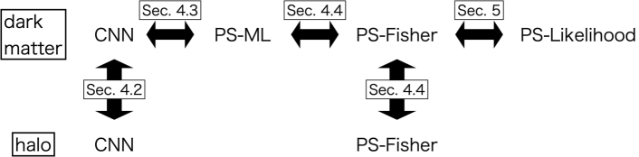
Figure 2: Here we show an overview of our work, highlighting the various comparisons between the different reconstruction methods. PS stands for the power spectrum, ML for machine learning, and CNN for convolutional neural network.

	DM	halo (all)	halo	DM	DM	halo
	CNN	CNN	CNN	PS-ML	PS-Fisher	PS-Fisher
$z=0.75$	3.8	3.9	4.5	2.3	1.4	0.42
$1.25$	2.3	2.2	2.5	2.0	1.7	0.63
$1.75$	1.2	1.1	1.7	2.7	1.7	0.67
$2.5$	0.74	1.2	1.2	2.9	1.5	0.61

($\times 10^{-2}$)

Table 2: The predicted errors on the $f\sigma_{8}$ quantity as derived by different methods. The first row shows the target of each analysis, i.e. DM (halo) means the analysis of the dark matter (halo) distribution, and halo (all) means we use the images including all halos. The second row shows the method of the analysis and each name corresponds to the one in Fig. 2. Every line from the third to sixth corresponds to each redshift from 0.75 to 2.5, and the components in this table show the values of the error divided by $10^{-2}$ for each method.

In this section, we describe the ML approach to extract cosmological parameters from images of the density field or the measured power spectra using the Quijote simulation. We first provide a basic structure of the ML architecture which is specifically optimized for image analysis and power spectrum analysis. We then show results in comparison with various different methodologies. Given the available dataset, we have established a set of comparison ladder: i.e. we first compare the result of CNN on dark matter density field images to those on the halo density field images (Sec. 4.2). This will directly compare the ability to constrain $f\sigma_{8}$ between dark matter and halo. We then compare the result of CNN on dark matter with ML-based dark matter power spectrum result (Sec. 4.3). This enables us to isolate the extra information content of the image which is not included in the power spectrum. Finally, we compare the ML-based dark matter power spectrum result with the Fisher matrix analysis (Sec. 4.4) or the conventional likelihood inference (Sec. 5) to see the advantages of the ML approach in terms of the constraining accuracy on $f\sigma_{8}$ as well as the possible systematic biases on the measurement.

The whole comparison ladder between the different methods is summarized in Fig. 2, while the predicted errors on the $f\sigma_{8}$ quantity as derived by different methods are then given in Table 2. In what follows, we proceed to discuss in detail how the analysis is performed for each method and how we perform the measurements in each case.

4.1 ML architecture

	Layer	Output map size
1	Input	$40\times 40\times 40\times 1$
2	$3\times 3\times 3$ convolution	$38\times 38\times 38\times 2$
3	BatchNorm3d	$38\times 38\times 38\times 2$
4	$2\times 2\times 2$ MaxPool	$19\times 19\times 19\times 2$
5	$2\times 2\times 2$ convolution	$18\times 18\times 18\times 64$
6	BatchNorm3D	$18\times 18\times 18\times 64$
7	$2\times 2\times 2$ MaxPool	$9\times 9\times 9\times 64$
8	$3\times 3\times 3$ convolution	$7\times 7\times 7\times 64$
9	$3\times 3\times 3$ convolution	$5\times 5\times 5\times 64$
10	$2\times 2\times 2$ convolution	$4\times 4\times 4\times 128$
11	BatchNorm3d	$4\times 4\times 4\times 128$
12	Flatten	$8192(=4^{3}\times 128)$
13	FullyConnected	$512$
14	FullyConnected	$256$
15	FullyConnected	$1$

Table 3: Our CNN architecture. In all convolutional layers, stride $=1$ and padding is not applied. Output map size corresponds to (height, width, depth, and channel). After each convolution layer and FullyConnected layer except for the last layer, we apply the ReLU as the activation function. The total number of trainable parameters is 5,345,341.

	Layer	Output size
1	Input	$3\times 39$
2	FullyConnected	$512$
3	FullyConnected	$512$
4	FullyConnected	$512$
5	FullyConnected	$512$
6	FullyConnected	$1$

Table 4: Our neural network architecture. After each FullyConnected layer except for the last layer, we apply the dropout layer with rates of $0.1$. The total number of trainable parameters is $848,897$.

In this work, we use the 3-dimensional CNN for the analysis of the images and a NN for the power spectrum. We used the publicly available platform PyTorch [45] to construct our CNN and NN and the architecture based on Ref. [46], however, note that some hyperparameters are different from those of that work, as the size of input data is different. In Table 3 and Table 4, we show the architecture of our CNN, while it should be noted that for the activation function, we apply the ReLU after each convolution layer and FullyConnected layer except for the last layer. Also, our CNN predicts the value of $f\sigma_{8}(z)$ from the $40\times 40\times 40$ image of dark matter or halo distribution introduced in Sec. 3.2.

Here we also use the mini-batch learning and when we choose $N_{b}$ as the batch size, we randomly divide the training data into groups, and each group has $N_{b}$ training data. This group is called a mini-batch and then, the average value of the loss function in the mini-batch is used to update the trainable parameters. With trial and error, we determined that the optimal batch size is $16$, note however that if we make the batch size unity (online learning), the loss value does not converge because we use batch normalization in our CNN.

As our main loss function we use the Mean Squared Error (MSE)

$$\mathcal{L}=\frac{1}{N_{b}}\sum_{i=1}^{N_{b}}(y_{i}-\hat{y}_{i})^{2},$$ (4.1)

where $N_{b}$ is the batch size, $y_{i}$ is the predicted value of $f\sigma_{8}$ from our CNN for the $i$-th data in the mini-batch data, and $\hat{y}_{i}$ is the ground-truth value, i.e. the correct $f\sigma_{8}$ value.

In updating the trainable parameters, we use the Adam optimizer, which is defined as torch.optim.Adam() in Pytorch. We use $5\times 10^{-7}$ and 0.1 as the value of lr and weight_decay which are the arguments of torch.optim.Adam(), respectively. The batch normalization is used in our CNN as we have found that this improves the efficiency of the learning. This is defined as torch.nn.BatchNorm3d() in PyTorch and we use the default values for all parameters.

And then, our NN predicts the value of $f\sigma_{8}$ from the Legendre expanded power spectrum. We use the $P_{0}(k)$, $P_{2}(k)$, and $P_{4}(k)$ for $k\leq 0.25$, so the size of input data to our NN is $3\ (P_{0},\ P_{2},\ \mathrm{and}\ P_{4})\times 39\ (\mathrm{the\ number\ of\ k\textrm{-}bins})$. Furthermore, we apply the dropout layer with the rate of 0.1 after each Fully Connected layer, except for 6th layer, see Table 4.

Finally, as the loss function and the optimizer of the trainable parameters, we use the MSE and the Adam optimizer where lr$=5\times 10^{-6}$ and weight_decay$=0$. In addition, we apply $N_{b}=16$ as the batch-size in training.

4.2 CNN results on dark matter and halo

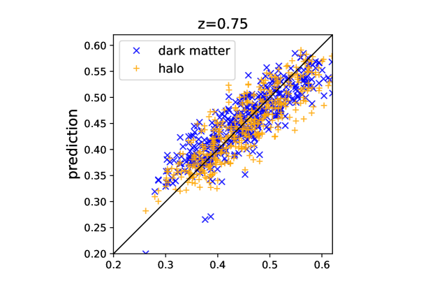
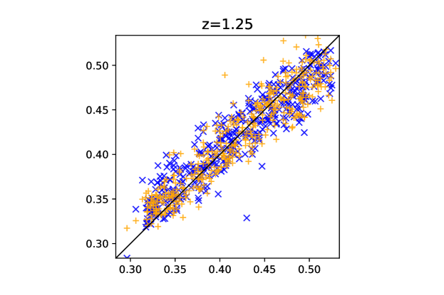
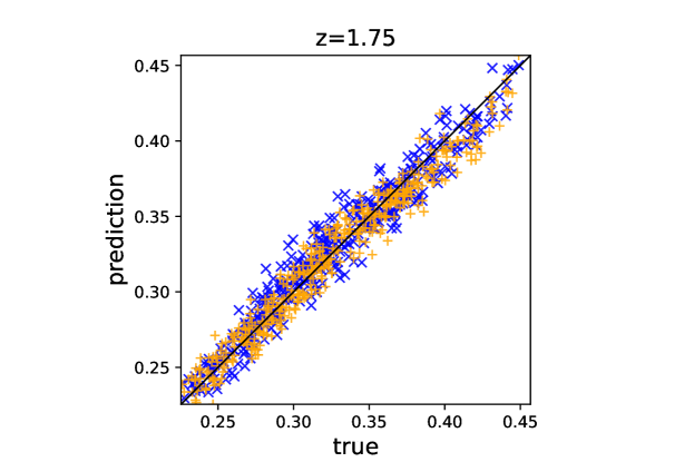
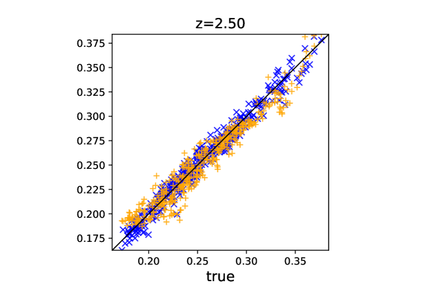
Figure 3: The results of our CNN for dark matter images (blue) and halo images, including all halo (orange) for each redshift. The horizontal axis shows the true value of $f\sigma_{8}$, and the vertical axis shows the predicted value of $f\sigma_{8}$ by our CNN.

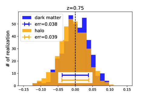
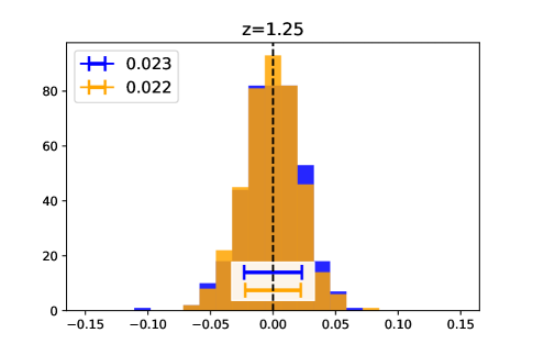
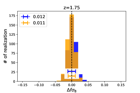
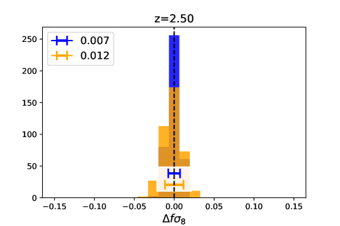
Figure 4: The histograms of the CNN prediction for dark matter images (blue) and halo images (orange) for each redshift bin. The horizontal axis corresponds to the value of $\Delta f\sigma_{8}$ predicted by our CNN, and the vertical axis shows the number of test images for each $\Delta f\sigma_{8}$. The error bars show the standard deviation of $\Delta f\sigma_{8}$, and its value is shown in the legend.

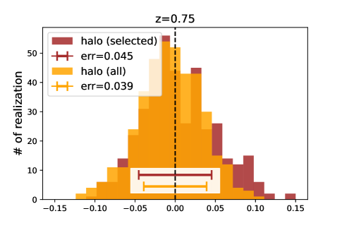
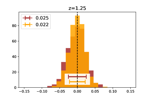
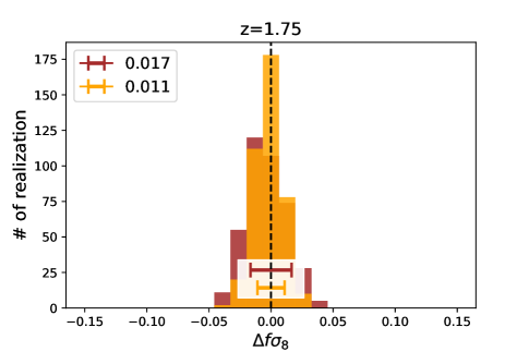
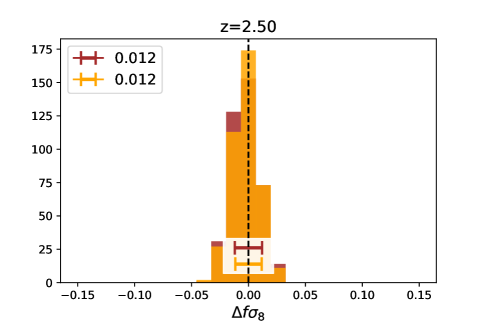
Figure 5: The results of our CNN for images including all halos (orange) and randomly selected halos (brown) for each redshift bin. The horizontal axis corresponds to the value of $\Delta f\sigma_{8}$ predicted by our CNN and the vertical axis shows the number of the test images for each $\Delta f\sigma_{8}$. The error bars show the standard deviation of $\Delta f\sigma_{8}$ and its value is shown in the legend.

In this subsection, we compare the results from our CNN for the images of dark matter distribution and the halo distribution.

In the training part, we train our CNN over $100$ epochs, where an epoch means the number of times our CNN trained by all training data. And then, in the test phase, we use the CNN model which minimizes the value of the loss function for the validation data.

In this work, the errors are estimated by the standard deviation of the vector of $\Delta f\sigma_{8,i}=(y_{\mathrm{pred},i}-y_{\mathrm{true},i})$, where $y_{\mathrm{pred},i}$ and $y_{\mathrm{true},i}$ are the CNN prediction and the ground truth for the $i$-th test data, respectively.

The validity of this estimation is confirmed as follows.

• We make a $30\times 30$ grid of parameters for $\Omega_{m}\in[0.1,0.5]$ and $\sigma_{8}\in[0.6,1.0]$.

• For each redshift, we evaluate the $f\sigma_{8}$ in the whole grid and then, we pick 400 grid points (this is the same number of the test data for our CNN) from them.

• We make the fake CNN predictions based on Gaussian with error $\sigma$.

• We compare the predicted error from the standard deviation of $\Delta f\sigma_{8,i}$ vector with fiducial error.

Figures 3 and 5 show the relation between true and predicted $f\sigma_{8}$ and $\Delta f\sigma_{8}$ for our CNN results for dark matter (blue) and halo (orange) images, respectively. For comparison purposes, here we use all halos in making images without throwing away halos. The horizontal axis corresponds to $\Delta f\sigma_{8}$, and the vertical axis shows the number of test images for each $\Delta f\sigma_{8}$. By comparing the results for dark matter images and halo images, we find that the errors are mostly comparable for all redshift bins, while the results for the dark matter images are better for $z=2.5$.

For both dark matter and halo images, we find that the error decreases when the redshift becomes larger. It is one of the possibilities that the non-linearities make it more difficult to extract the information from the matter distribution at the low redshift. At $z=2.5$, the error for the halo images is larger than the one for the dark matter and comparable to the one for $z=1.75$ halo images. We can consider that it is caused by the shot noise because the halo number in the simulation at $z=2.5$ is less than one-tenth of the other redshift in using all halos.

Next, we investigate the effect of the random selection of the halos. Instead of the images including all halos, we reduce the number of halos so that its redshift distribution follows realistic observation (the ratio is shown in Table 1) and use them to train and test our CNN, and the results are shown in Fig. 4. Even when we use only randomly selected halos, we can see the redshift dependence of the error in the same as the all-halo case. The errors of the selected-halo case are larger than the ones for all halos, but this is reasonable because the images of the selected halos lose the information compared to the images including all halos.

We additionally performed some tests in the CNN architecture by exploring different loss functions in order to corroborate our results. We studied the CNN behavior with MSE Loss, MAE (Mean Squared Error) Loss, Hubber Loss, and the moments network Loss (LFI) [47, 48]. The MSE Loss calculates the mean squared error between the CNN estimates, and the true values and is set up to find an approximation of the marginal posterior mean. The advantage of LFI with respect to the other loss functions is that it achieves a better convergence between the CNN output and both: the mean $\mu_{i}$ and standard deviation $\sigma_{i}$ of the marginal posterior parameters $\theta_{i,j}$. According to the mentioned arguments, LFI Loss is defined by [49]:

$$\mathcal{L}_{\mathrm{LFI}}=\sum_{i=1}^{6}\log\left(\sum_{j\in\text{ batch }}\left(\theta_{i,j}-\mu_{i,j}\right)^{2}\right)+\sum_{i=1}^{6}\log\left(\sum_{j\in\text{ batch }}\left(\left(\theta_{i,j}-\mu_{i,j}\right)^{2}-\sigma_{i,j}^{2}\right)^{2}\right).\\$$ (4.2)

As a matter of interest, we found a similar outcome with all the considered Loss functions - an error decrease for larger redshifts. It is worth mentioning that LFI performs better, as expected. In Table 5 we show the results only for the MSE and LFI Loss functions for simplicity, where we see that the LFI indeed improves the error estimates compared to the previously considered MSE Loss function.

z	MSE Loss	LFi Loss
0.75	3.2	1.8
1.25	2.3	1.5
1.75	1.1	0.9
2.5	1.2	1.0

($\times 10^{-2}$)

Table 5: Predicted errors for each redshift snapshot using Mean Squared Error (MSE) Loss and the moments networks Loss (LFI) Functions in the CNN architecture.

4.3 ML-based power spectrum analysis on dark matter

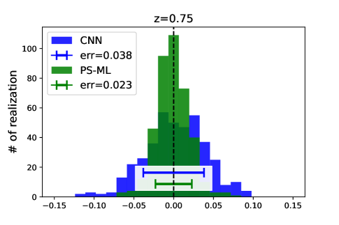
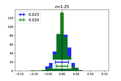
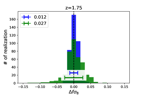
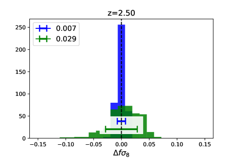
Figure 6: The results of our CNN for dark matter images (blue) and PS-ML (green) for each redshift bin. The horizontal axis correspond to the value of $\Delta f\sigma_{8}$ predicted by our CNN and PS-ML, and the vertical axis shows the number of the test images for each $\Delta f\sigma_{8}$. The error bars show the standard deviation of $\Delta f\sigma_{8}$ and it’s value is shown in the legend.

Now we compare the results for the ML-based power spectrum (PS-ML) analysis with the one from our CNN for dark matter. In this subsection, we use the NN whose architecture is shown in Table 4 for the power spectrum analysis. In training, we train our NN over 3,000 epochs. And then, in the test, we use the NN model which minimizes the value of the loss function for the validation data. The method of the estimation of the error is the same as the one for our CNN in Sec. 4.2.

In Fig. 6 we compare the results obtained by dark matter images (blue, same as the one in Fig. 5) and PS-ML (green). At the lowest redshift, the error by the CNN analysis is larger than the one by PS-ML. We also find that the errors by PS-ML do not largely depend on redshift, unlike the CNN analysis. So at higher redshifts ($z>1.75$), our CNN can predict $f\sigma_{8}$ more precisely.

4.4 Comparison with a Fisher analysis

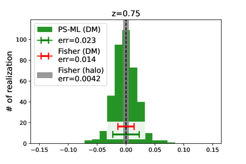
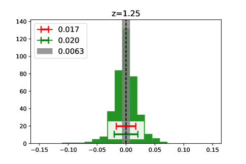
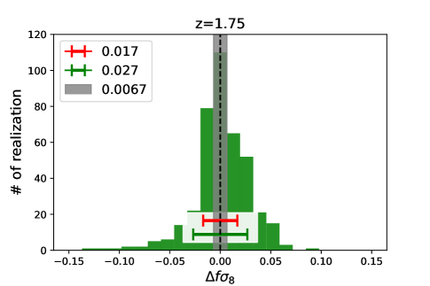
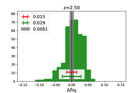
Figure 7: The results of PS-ML (green, same as Figure 6) for each redshift, plotted togather with the errors from the Fisher analysis for the power spectrum of dark matter (red) and the one of halo (gray-shaded). The horizontal axis corresponds to the value of $\Delta f\sigma_{8}$ predicted, and the vertical axis shows the number of the test images for each $\Delta f\sigma_{8}$.

In this subsection, we compare the results for the ML-based power spectrum analysis in Sec. 4.3 and the Fisher analysis described in Sec. 2.2. The results are shown in Fig. 7. Here, the errors of the Fisher analysis for halo are computed by using the bias shown in equation (2.28), and the one for dark matter is calculated for $b=1$.

For the analysis of dark matter distribution, both of the errors calculated by the ML-based and Fisher analysis do not largely depend on redshift. In addition, the errors from the Fisher analysis is smaller than the one from the ML-based analysis. This means there is a possibility that PS-ML does not access all the information included in power spectra, and there is room for improvement on our NN architecture.

In Fig. 7, the gray-shaded region shows the errors from the Fisher analysis for halo distribution and this error is smaller than the one for dark matter. This could be because the shot noise affects the analysis. As we can find from the halo bias Eq. (2.28), the amplitude of the halo power spectrum is larger than the one for dark matter. Therefore, the effect of the shot noise on the halo analysis is smaller relative to the dark matter analysis.

4.5 Effect of the random seed

Finally, we discuss the effect of the random initial conditions. So far, we have used the set of Latin-hypercube Quijote simulations, and these simulations have different random seeds for the initial conditions. Therefore, the difference in these simulations is caused by the difference in both its cosmological parameters and its initial condition. To discuss the effect of the latter, we use another dataset of Quijote simulations. The Quijote simulations have 15,000 realizations as ‘Fid’ simulations for the same cosmological parameter set and different random seeds for their initial conditions.

First, we pick up 400 realizations randomly from the ‘Fid’ simulation dataset and make the 3D images of halo distribution from these data following Sec. 3.2. And then, we test our CNN model for halo images, trained in Sec. 4.2, using the images from the ‘Fid’ simulations. By doing this, we can see the error only from random initial conditions. As a result, we find that the error for ‘Fid’ realizations is about 0.005 regardless of the redshift. This is about one-fifth of the error in the results in the previous subsections, which includes both effects from the cosmological parameters and the initial condition. Therefore, we conclude the error in our analysis is dominated by the difference in the cosmological parameters.

5 Comparison to the conventional likelihood inference

Here we compare the results from the CNN and ML-based power spectrum analysis to the likelihood-based parameter inference, which is widely adopted in the literature. To avoid any uncertainty in the theoretical model, we use the set of Latin-hypercube Quijote simulation outputs as a well-calibrated model. We first measure the covariance matrix from 15,000 realizations for the fiducial cosmological parameter set. Also, we consider the power spectrum averaged over 15,000 realizations as the observed data, where the fluctuations caused by the cosmic variance are eliminated. In a practical situation, the data include the cosmic variance uncertainty and but the model does not. However, given the available dataset of Quijote simulations, we include the cosmic variance uncertainty in the model.

Given the magnitude of the covariance errors, which corresponds to the 1 $[h^{-1}{\rm Gpc}]^{3}$ survey volume, we find that the sampling rate of the Latin-hypercube simulations is too sparse to correctly sample the cosmological parameter. Therefore, we linearly interpolate the power spectra in the 6 dimension cosmological parameters, namely the 5 parameters listed in the Eqs. (3.1) and $f\sigma_{8}(z)$. To test the interpolation accuracy, we first generate the interpolation table using 1,600 random samples from Latin-hypercube simulations and then compare the interpolated power spectra at the locations of the rest of 400 sets of cosmological parameters. We find that the interpolated power spectra recover the measured power spectra within $\sim$10% accuracy including the cosmic variance at all scales $k<0.4{\rm Mpc}^{-1}h$.

Using those well-reproduced interpolated model, we find the best-fitting parameters in the parameter vector of {$\Omega_{m}$, $h$, $n_{s}$, $\sigma_{8}$, $f\sigma_{8}$}, using a Markov Chain Monte Carlo (MCMC) analysis, with the publicly available code, emcee. In Fig. 8 we show the obtained one dimensional likelihood marginalized over other parameters. The best-fitting value of $f\sigma_{8}$ is slightly higher than the fiducial value, but it is well within the 1$\sigma$ region. Also, the measured error is slightly smaller than the Fisher matrix prediction in Sec. 4.4.

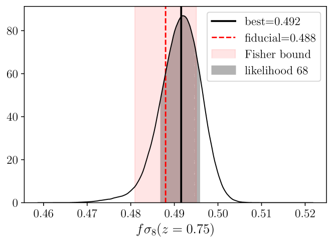
Figure 8: Bound on the $f\sigma_{8}$ parameter from a MCMC analysis. The black vertical line shows the best-fitting value and the black shaded region is the 1$\sigma$ range, while red dashed vertical line shows the fiducial value of the simulation and the red shaded region is a prediction from the Fisher analysis.

6 Discussions and conclusions

The growth-rate of matter density perturbations, described by the bias-independent $f\sigma_{8}(z)$ quantity, is an important quantity in the study of the large scale structure of the Universe, as it allows us to probe the dynamic features of gravity. However, in order to extract $f\sigma_{8}(z)$ from observations made by galaxy surveys two key assumptions have to be made: i) a fiducial cosmological model and ii) the modeling of the non-linear part of the power spectrum. From these two assumptions, the latter is particularly insidious as currently only purely phenomenological models exist in the literature, thus potential biasing the measurements of $f\sigma_{8}(z)$ in ways that are not easy to correct a posteriori.

In this work we use a particular ML approach based on training CNNs on the N-body simulations in order to extract $f\sigma_{8}(z)$ from galaxy surveys without having to assume any particular modelling of the non-linearities of the power spectrum. In a sense we perform a likelihood-free extraction of the growth rate by taking advantage of the ability of the neural network architecture to predict the growth $f\sigma_{8}(z)$ from images of the dark matter or halo distributions as discussed in Sec. 4.1.

Specifically, in our work we followed a multi-pronged approach in order to find the optimal way to extract the growth via a ML architecture. Also, in order to validate our approach we performed a standard Fisher matrix analysis by assuming an ideal and fiducial survey motivated by the Quijote simulations, i.e. having the same number of redshifts bins and covering an area in the sky corresponding to the angle subtended by a box of the simulations.

We summarize our overall approach in Fig. 2, while the main results and comparisons between the various approaches are shown in Figs. 3, 4, 5, 6 and 7, where we showed scatter plots and histograms comparing the CNN dark matter and halo reconstructions, the CNN dark matter and PS-ML reconstructions and finally, the PS-ML and Fisher matrix approach. The predicted errors from all approaches are also shown in Table 2.

Overall, as can be seen in the aforementioned figures and Table 2, we find that the ML-architecture can predict quite accurately the value of the growth rate $f\sigma_{8}(z)$, while the reconstructed errors from the CNN are comparable within a factor of order unity between the different ML approaches based on the DM or halo catalogs.

When comparing the ML results to the Fisher matrix approach for a fiducial survey based on specifications inspired from the Quijote simulations, we find that the Fisher results for the errors are quite optimistic. Specifically, we found a factor of reduction of two for low redshifts compared to the CNN DM results and a factor of two to ten for the halo results. The latter result could be due to the fact that the Fisher in this case integrates over many more Fourier modes of the perturbations, thus has more information, which in principle might not be accessible to the CNN. Also, in the case of the Fisher matrix approach we observe no reduction in the errors with increasing errors, instead the errors seem to track well the assumed redshift distribution of the ideal survey sample.

One plausible reason for the redshift trend of the CNN results and the deviation from the Fisher results, might be that at low redshifts the enhanced non-linearities might introduce more scatter in the observed by the CNN values of $f\sigma_{8}$, something which might not be captured correctly by the Fisher matrix approach which uses a phenomenological approach for the non-linearities. Instead the Fisher matrix approach errors seem to follow the redshift distribution of objects for the ideal survey sample and ignore the more complicated non-linear regime at low redshifts.

So, in order to investigate the differences from the Fisher matrix approach and the observed redshift trend for the DM and Halo CNN results, we performed several tests. First, we examined the effect of the random selection of the halos, by making images that have a part of halos to reproduce the relative number shown in Table 1 and then used them to train and test our CNN. Doing so we found the same redshift dependence of the error as in the previous case. Second, we also explored different loss functions, including the MSE, MAE, Hubber Loss and LFI loss functions. Overall, we found a similar decrease in the error with redshift, but the LFI function displays an improvement in the error estimates with respect to the MSE loss function. Third, we investigated the effect of the random initial conditions by using another dataset of Quijote simulations. Doing so we find that the error contribution is only one-fifth of the total error, thus we conclude that the error in our analysis is dominated by the difference in the cosmological parameters.

We leave for future work the extension of this analysis to models beyond the $\Lambda$CDM model, i.e. to eliminate the first assumption of current growth measurements as mentioned earlier since that requires N-body simulations for modified gravity. Also, we leave for future work a more detailed comparison between the CNN and the Fisher matrix approach, as it would require significant theoretical modifications on the non-linear part for the latter, and more tests on the CNN architecture to investigate the effect on low redshifts.

Finally, given that in a few years the forthcoming galaxy surveys will provide a plethora of high-quality data related to the large-scale structure of the Universe, novel ways to analyse these data will be required in order to minimize the theoretical errors emanating from assumptions, just as the non-linear modeling at small scales. Here we provided the first step in this direction, but more work will be required to bridge the gap between the theory and the actual data.

References

- [1] T. Padmanabhan, Cosmological constant—the weight of the vacuum, Physics Reports 380 (2003) 235.
- [2] L. Amendola, V. Marra and M. Quartin, Internal robustness: systematic search for systematic bias in sn ia data, Monthly Notices of the Royal Astronomical Society 430 (2013) 1867.
- [3] Planck collaboration, Planck 2018 results. VI. Cosmological parameters, Astron. Astrophys. 641 (2020) A6 [1807.06209].
- [4] DES collaboration, Dark Energy Survey Year 3 results: Cosmological constraints from galaxy clustering and weak lensing, Phys. Rev. D 105 (2022) 023520 [2105.13549].
- [5] T. Kacprzak and J. Fluri, Deeplss: breaking parameter degeneracies in large scale structure with deep learning analysis of combined probes, arXiv preprint arXiv:2203.09616 (2022) .
- [6] EUCLID collaboration, Euclid Definition Study Report, 1110.3193.
- [7] LSST Science, LSST Project collaboration, LSST Science Book, Version 2.0, 0912.0201.
- [8] DESI collaboration, The DESI Experiment Part I: Science,Targeting, and Survey Design, 1611.00036.
- [9] A. Joyce, L. Lombriser and F. Schmidt, Dark Energy Versus Modified Gravity, Ann. Rev. Nucl. Part. Sci. 66 (2016) 95 [1601.06133].
- [10] V. Motta, M.A. García-Aspeitia, A. Hernández-Almada, J. Magaña and T. Verdugo, Taxonomy of Dark Energy Models, Universe 7 (2021) 163 [2104.04642].
- [11] A. Lazanu, Extracting cosmological parameters from n-body simulations using machine learning techniques, Journal of Cosmology and Astroparticle Physics 2021 (2021) 039.
- [12] F. Villaescusa-Navarro, C. Hahn, E. Massara, A. Banerjee, A.M. Delgado, D.K. Ramanah et al., The quijote simulations, The Astrophysical Journal Supplement Series 250 (2020) 2.
- [13] V. Desjacques, D. Jeong and F. Schmidt, Large-Scale Galaxy Bias, Phys. Rept. 733 (2018) 1 [1611.09787].
- [14] B. Sagredo, S. Nesseris and D. Sapone, Internal robustness of growth rate data, Physical Review D 98 (2018) 083543.
- [15] Y.-S. Song and W.J. Percival, Reconstructing the history of structure formation using redshift distortions, Journal of Cosmology and Astroparticle Physics 2009 (2009) 004.
- [16] WiggleZ collaboration, The WiggleZ Dark Energy Survey: measuring the cosmic growth rate with the two-point galaxy correlation function, Mon. Not. Roy. Astron. Soc. 430 (2013) 924 [1302.5178].
- [17] R. Scoccimarro and J. Frieman, Loop corrections in nonlinear cosmological perturbation theory, Astrophys. J. Suppl. 105 (1996) 37 [astro-ph/9509047].
- [18] F. Bernardeau, N. Van de Rijt and F. Vernizzi, Resummed propagators in multi-component cosmic fluids with the eikonal approximation, Phys. Rev. D 85 (2012) 063509 [1109.3400].
- [19] T. Baldauf, M. Mirbabayi, M. Simonović and M. Zaldarriaga, Equivalence Principle and the Baryon Acoustic Peak, Phys. Rev. D 92 (2015) 043514 [1504.04366].
- [20] S. Casas, M. Kunz, M. Martinelli and V. Pettorino, Linear and non-linear Modified Gravity forecasts with future surveys, Phys. Dark Univ. 18 (2017) 73 [1703.01271].
- [21] Euclid collaboration, Euclid preparation: VII. Forecast validation for Euclid cosmological probes, Astron. Astrophys. 642 (2020) A191 [1910.09273].
- [22] S. Nesseris, G. Pantazis and L. Perivolaropoulos, Tension and constraints on modified gravity parametrizations of from growth rate and Planck data, Phys. Rev. D 96 (2017) 023542 [1703.10538].
- [23] L. Kazantzidis, L. Perivolaropoulos and F. Skara, Constraining power of cosmological observables: blind redshift spots and optimal ranges, Phys. Rev. D 99 (2019) 063537 [1812.05356].
- [24] A. Lazanu, Extracting cosmological parameters from N-body simulations using machine learning techniques, JCAP 09 (2021) 039 [2106.11061].
- [25] Z. Wu, L. Xiao, X. Xiao, J. Wang, X. Kang, Y. Wang et al., AI-assisted reconstruction of cosmic velocity field from redshift-space spatial distribution of halos, 2301.04586.
- [26] F. Qin, D. Parkinson, S.E. Hong and C.G. Sabiu, Reconstructing the cosmological density and velocity fields from redshifted galaxy distributions using V-net, 2302.02087.
- [27] C.-P. Ma and E. Bertschinger, Cosmological perturbation theory in the synchronous and conformal newtonian gauges, arXiv preprint astro-ph/9506072 (1995) .
- [28] F. Bernardeau, S. Colombi, E. Gaztanaga and R. Scoccimarro, Large-scale structure of the universe and cosmological perturbation theory, Physics reports 367 (2002) 1.
- [29] S. Nesseris, The effective fluid approach for modified gravity and its applications, Universe 9 (2022) 13.
- [30] H. Kurki-Suonio, Cosmological perturbation theory, unpublished lecture notes available: http://theory. physics. helsinki. _/cmb/(referenced 23 Oct. 2005) (2005) .
- [31] S. Tsujikawa, Matter density perturbations and effective gravitational constant in modified gravity models of dark energy, Physical Review D 76 (2007) 023514.
- [32] T. Padmanabhan, Cosmological constant-the weight of the vacuum, Physics Report 380 (2003) 235 [hep-th/0212290].
- [33] V. Silveira and I. Waga, Decaying Lambda cosmologies and power spectrum, Phys. Rev. D 50 (1994) 4890.
- [34] W.J. Percival, Cosmological structure formation in a homogeneous dark energy background, Astron. Astrophys. 443 (2005) 819 [astro-ph/0508156].
- [35] A. Bueno belloso, J. Garcia-Bellido and D. Sapone, A parametrization of the growth index of matter perturbations in various Dark Energy models and observational prospects using a Euclid-like survey, JCAP 10 (2011) 010 [1105.4825].
- [36] X.-D. Li, H. Miao, X. Wang, X. Zhang, F. Fang, X. Luo et al., The redshift dependence of the alcock–paczynski effect: Cosmological constraints from the current and next generation observations, The Astrophysical Journal 875 (2019) 92.
- [37] X.-D. Li, C.G. Sabiu, C. Park, Y. Wang, G.-b. Zhao, H. Park et al., Cosmological constraints from the redshift dependence of the alcock–paczynski effect: dynamical dark energy, The Astrophysical Journal 856 (2018) 88.
- [38] L. Kazantzidis and L. Perivolaropoulos, Evolution of the tension with the Planck15/CDM determination and implications for modified gravity theories, Phys. Rev. D 97 (2018) 103503 [1803.01337].
- [39] E. Macaulay, I.K. Wehus and H.K. Eriksen, Lower Growth Rate from Recent Redshift Space Distortion Measurements than Expected from Planck, Phys. Rev. Lett. 111 (2013) 161301 [1303.6583].
- [40] M. Tegmark, Measuring cosmological parameters with galaxy surveys, Phys. Rev. Lett. 79 (1997) 3806 [astro-ph/9706198].
- [41] H.-J. Seo and D.J. Eisenstein, Probing dark energy with baryonic acoustic oscillations from future large galaxy redshift surveys, Astrophys. J. 598 (2003) 720 [astro-ph/0307460].
- [42] S. Yahia-Cherif, A. Blanchard, S. Camera, S. Casas, S. Ilić, K. Markovic et al., Validating the Fisher approach for stage IV spectroscopic surveys, Astron. Astrophys. 649 (2021) A52 [2007.01812].
- [43] J. Lesgourgues, The Cosmic Linear Anisotropy Solving System (CLASS) I: Overview, 1104.2932.
- [44] D. Blas, J. Lesgourgues and T. Tram, The Cosmic Linear Anisotropy Solving System (CLASS) II: Approximation schemes, JCAP 07 (2011) 034 [1104.2933].
- [45] A. Paszke, S. Gross, F. Massa, A. Lerer, J. Bradbury, G. Chanan et al., Pytorch: An imperative style, high-performance deep learning library, in Advances in Neural Information Processing Systems 32, H. Wallach, H. Larochelle, A. Beygelzimer, F. d'Alché-Buc, E. Fox and R. Garnett, eds., pp. 8024–8035, Curran Associates, Inc. (2019), http://papers.neurips.cc/paper/9015-pytorch-an-imperative-style-high-performance-deep-learning-library.pdf.
- [46] A. Lazanu, Extracting cosmological parameters from N-body simulations using machine learning techniques, JCAP 2021 (2021) 039 [2106.11061].
- [47] F. Villaescusa-Navarro, S. Genel, D. Angles-Alcazar, L. Thiele, R. Dave, D. Narayanan et al., The camels multifield data set: Learning the universe’s fundamental parameters with artificial intelligence, The Astrophysical Journal Supplement Series 259 (2022) 61.
- [48] N. Jeffrey and B.D. Wandelt, Solving high-dimensional parameter inference: marginal posterior densities & moment networks, arXiv preprint arXiv:2011.05991 (2020) .
- [49] L.A. Perez, S. Genel, F. Villaescusa-Navarro, R.S. Somerville, A. Gabrielpillai, D. Anglés-Alcázar et al., Constraining cosmology with machine learning and galaxy clustering: the camels-sam suite, arXiv preprint arXiv:2204.02408 (2022) .
- [50] P. Virtanen, R. Gommers, T.E. Oliphant, M. Haberland, T. Reddy, D. Cournapeau et al., SciPy 1.0: Fundamental Algorithms for Scientific Computing in Python, Nature Methods 17 (2020) 261.
- [51] C.R. Harris, K.J. Millman, S.J. van der Walt, R. Gommers, P. Virtanen, D. Cournapeau et al., Array programming with NumPy, Nature 585 (2020) 357.
- [52] J.D. Hunter, Matplotlib: A 2d graphics environment, Computing in Science & Engineering 9 (2007) 90.