The total spine of the Milnor fibration of a plane curve singularity

Abstract

We study the separatrices at the origin of the vector field $-\nabla\log|f|$, where $f$ is any plane curve singularity. Under some genericity conditions on the metric, we produce a natural partition of the set of separatrices, $S$, into a finite collection smooth strata. As a byproduct of this theory, we construct a smooth fibration which is equivalent to the Milnor fibration, and lives on a quotient of the Milnor fibration at radius $0$. The strict transform of $S$ in this space induces a spine for each fiber of this fibration. These fibers are endowed with a vector field in such a way that the spine consists of trajectories which do not escape through the boundary.

1 Introduction

Motivation

The motivation for this work comes from a question that Thom posed to Lê [Lê88]. More concretely, let $f:\mathbb{C}^{n}\to\mathbb{C}$ be a holomorphic map. Then there exists $\varepsilon,\eta>0$ with $\varepsilon$ small enough and $\eta$ small with respect to $\varepsilon$ such that the restriction of $f$ yields a locally trivial fibration:

(1.0.1) $$f|_{B_{\varepsilon}\cap f^{-1}(D_{\eta})^{*}}:B_{\varepsilon}\cap f^{-1}(D_{\eta}^{*})\to D_{\eta}^{*}$$

This is the Milnor fibration over the punctured disk. The following two results were proven by Milnor [Mil68]

1. The pair of spaces $(f^{-1}(0)\cap B_{\varepsilon},B_{\varepsilon})$ is homeomorphic to the pair of cones $(C(f^{-1}(0)\cap S_{\varepsilon}),C(S_{\varepsilon}))$.

2. When $f$ has an isolated critical point at the origin, the Milnor fiber $F$ has the homotopy type of a bouquet of spheres of real dimension $n-1$.

In this context, according to [Lê88], Thom asked Lê if one could find a polyhedron $P$ contained in this fibre $F$ (the Milnor fiber), of real dimension $n-1$, such that $F$ would be a regular neighborhood of $P$. From this result one would obtain the construction of a continuous application which would send $F$ to the special fibre $F_{0}$, sending $P$ to $\{0\}$ and $F\setminus P$ homeomorphically to $F_{0}\setminus\{0\}$. This application would geometrically realize the collapsing of the homology $H(F)$ of $F$ on the trivial homology of $F_{0}$ and this would give a geometric realization of the vanishing cycles of the function at the isolated critical point.

A solution to this problem in the more general context of germs of analytic maps with isolated singularity defined on analytic complex spaces $f:X\to\mathbb{C}$ was sketched by Lê in [Lê88] and later [LM17, Theorem 1], detailed by Lê and Menegon. More concretely, they proved the following: let $F_{t}$ be the Milnor fiber of $f$ and let $F_{0}$ be the central fiber. Then there exists a polyhedron $P_{t}\subset F_{t}$ of real dimension $\dim_{\mathbb{C}}F_{t}$ and a continuous simplicial map $\partial F_{t}\to P_{t}$ such that $F_{t}$ is homeomorphic to the mapping cylinder of the map above. Furthermore, there exists a continuous map of pairs $\Psi_{t}:(F_{t},P_{t})\to(F_{0},0)$ such that its restriction $F_{t}\setminus P_{t}\to F_{0}\setminus\{0\}$ is a homeomorphism. Their construction can be realized simultaneously only over a proper sector of the base space of the fibration, which is a punctured disk.

The starting point of our program is based on an original idea by A’Campo [A’C18] that can be summarized as follows:

1. Consider the inwards pointing radial vector field $-t/|t|$ on the disk $D_{\eta}$.

2. Lift the vector field to a vector field $\xi^{\mathrm{lift}}$ on $B_{\varepsilon}\setminus C$ using the connection given by the family of tangent planes which are the symplectic orthogonals to the vertical tangent bundle associated with the Milnor fibration.

3. Integrate the vector field and analyze the uniparametric family of diffeomorphisms that takes Milnor fibers along a ray all the way to the central fiber.

4. Analyze the maps $\rho_{t}:F_{t}\to f^{-1}(0)$ resulting from taking the limit of these diffeomorphisms and study the set $S_{t}=\rho_{t}^{-1}(0)\subset F_{t}$.

The set $S_{t}$ is the expected spine for the Milnor fiber $F_{t}$ but it is not clear, a priori, what kind of structure it has. At this moment a simple observation is due: Analyzing the set $S_{t}$ amounts to analyzing the separatrices at $0$ of $\xi^{\mathrm{lift}}$, that is, the set of integral lines $S$ of $\xi^{\mathrm{lift}}$ that converge to the origin. Intersecting this set with each Milnor fiber $S\cap F_{t}$ equally defines the set $S_{t}$. From now on, we consider the case of plane curves, that is, $n=2$. We do not assume, however, that the plane curve is isolated.

Our program parts from A’Campo’s idea but it quickly bifurcates. The lift of the vector field $-t/|t|$ is easily seen to be, up to multiplication by a positive real function, the vector field

$$\xi=-\nabla\log|f|.$$

In particular, $\xi$ and $\xi^{\mathrm{lift}}$ have the same integral lines. So this problem turns out to be closely related to the study of integral lines of gradients of absolute values of complex analytic maps.

The set $S$ is very complicated near the origin so a natural idea to study it, is to follow this strategy: blow up the origin

$$\pi_{0}:(Y_{0},\tilde{C}\cup D_{0})\to(\mathbb{C}^{2},C)$$

and see if the strict transform of the separatrices $\overline{\pi_{0}^{-1}(S)}$ intersects in a reasonable way the new exceptional divisor $D_{0}$. It happens that, under some genericity conditions on the metric, some of the trajectories in $S$ now meet $D_{0}$ transversely at a finite set of points $\Sigma_{0}$. Moreover, one is able to suitably rescale $\pi_{0}^{*}\xi$ in such a way that the rescaled vector field extends over $D_{0}^{\circ}=D_{0}\setminus\tilde{C}$ to a vector field $\hat{\xi}_{0}$ and its restriction $\xi_{0}=\hat{\xi}_{0}|_{D_{0}^{\circ}}$ satisfies that

1. $\xi_{0}$ is the gradient with respect to the Fubini-Study metric on $D_{0}$ of a Morse function $D_{0}^{\circ}\to\mathbb{R}$.

2. The critical set of $\xi_{0}$ is precisely $\Sigma_{0}$.

3. $\xi_{0}$ has fountain singularities and saddle points on interior points of $D_{0}^{\circ}$ but it does not have sink singularities.

4. The intersection points of $D_{0}$ with the strict transform $\tilde{C}$ behave like sink singularities, that is, $\xi_{0}$ points towards the strict transform near these intersection points.

While we have simplified our set $S$, the problem is far from being solved: there are still many trajectories in $\pi_{0}^{-1}(S)$ that converge to intersection points in $\tilde{C}\cap D_{0}$. Some wishful thinking leads one to believe that further repeating of this technique will eventually resolve the set $S$ and one shall be able to study these separatrices by studying some sort of nice Morse vector fields on the divisors $D_{i}$ of, let’s say, an embedded resolution $\pi:(Y,D=\bigcup_{i}D_{i})\to(\mathbb{C}^{2},C)$. This couldn’t be further from the truth since a lot of things that behave nicely on the first blow up, go wrong. In particular, it is not always possible to re-scale and extend the (pullback of) the vector field $\xi$ to the divisors $D_{i}$. This phenomenon occurs because the extension depends on the angle $\theta$ from which one approaches the origin. Once spotted the problem and its origin, it becomes natural to perform a real oriented blow up of the resolution space $Y$ along the exceptional set $D$. The real oriented blow up substitutes a manifold by the moduli of all the normal directions to this manifold. Note that the function $\arg(f)$ that gives the argument of $f$, is only well defined outside $C$. The real oriented blow up

$$\sigma:(Y^{\mathrm{ro}},D^{\mathrm{ro}})\to(Y,D)$$

resolves this indeterminacy: the function $\arg(f)$ lifts to a function $\arg^{\mathrm{ro}}(f)$ that naturally extends over all $Y^{\mathrm{ro}}$. With $\pi^{\mathrm{ro}}=\pi\circ\sigma$, this same phenomenon allows us to rescale and extend the vector field $(\pi^{\mathrm{ro}})^{*}\xi$ to vector fields $\xi^{\mathrm{ro}}_{i}$ that are defined on, and are tangent to, the exceptional divisors $D^{\mathrm{ro}}_{i}=\sigma^{-1}(D_{i})$.

The space $Y^{\mathrm{ro}}$ is a manifold with corners. As a topological manifold it has a boundary $\partial Y^{\mathrm{ro}}=D^{\mathrm{ro}}$ that fibers over the circle $\mathbb{R}/2\pi\mathbb{Z}$ via the map $\arg^{\mathrm{ro}}(f)$. This topological fibration is equivalent to the Milnor fibration and it is usually known as the Milnor fibration at radius $0$ and its fiber $F^{\mathrm{ro}}_{\theta}$ the Milnor fiber at radius $0$. This fibration was described by A’Campo [A’C75] to describe a zeta function for the monodromy. See also [KN99] for a very similar construction.

When the metric used to define $\xi$ satisfies other genericity conditions we show that the vector fields $\xi^{\mathrm{ro}}_{i}$ behave in a nice way:

1. $\xi^{\mathrm{ro}}_{i,\theta}=\xi^{\mathrm{ro}}_{i}|_{F^{\mathrm{ro}}_{\theta}\cap D^{\mathrm{ro}}_{i}}$ has a saddle-point singularity at a point $p\in D^{\mathrm{ro},\circ}_{i,\theta}$ if and only if $\sigma(p)\in D_{i}$ is the intersection point of the strict transform of a particular relative polar curve and $D_{i}$.

2. $\xi^{\mathrm{ro}}_{i,\theta}$ has no other singularities on $p\in D^{\mathrm{ro},\circ}_{i,\theta}$.

At this point we have simplified enough the set of separatrices $S$ and we conclude that it can be partitioned into manifolds of trajectories that converge either to some saddle point of some $\xi^{\mathrm{ro}}_{i,\theta}$ or to a repeller on the first blow up. More concretely:

Theorem A (Theorem 11.2.1).

Assuming that $\mathbb{C}^{2}$ is endowed with a generic metric, the punctured total spine $S\setminus\{0\}$ is the disjoint union of strata, each of which is a punctured disk, an open solid torus or an open solid Klein bottle. Each stratum corresponds to a point $p$ on the exceptional divisor of an embedded resolution of $(C,0)$, in that it is the union of trajectories of $\xi$ whose lift to the resolution converges to $p$.

In Section 12 we define the invariant Milnor fibration at radius zero which as a set, is a quotient of the Milnor fibration at radius zero.

Theorem B (Theorem 12.3.12).

The invariant Milnor fibration naturally admits a smooth structure and a smooth vector field tangent to each Milnor fiber. The union of trajectories of this vector field, which do not escape through the boundary, is a spine for each Milnor fiber. As a set, this spine coincides with the intersection of strict transform of the total spine with the Milnor fibration at radius zero. Moreover, this spine has the structure of a piecewise smooth $1$-dimensional CW complex and all the $1$-cells meet transversely at the $0$-cells

Note that we are able to construct this spine for all $\theta\in\mathbb{R}/2\pi\mathbb{Z}$ at the same time and so, necessarily, the topological type of the spine changes with $\theta$ because, otherwise, we would get a finite order algebraic monodromy which is not always the case for plane curve singularities.

Organization of the paper

In Section 2 we recall the ideas of A’Campo [A’C18] and motivate our problem. Using Łojasiewicz results [Łoj84], we prove that the ideas of A’Campo yield a well defined collapsing map

$$\rho_{t}:F_{t}\to V$$

from each Milnor fiber $t\in D_{\eta}^{*}$ to the central fiber $C$. We show that this map is a local diffeomorphism when restricted outside the preimage of the origin. One of the main goals of the rest of the paper is to understand the set

$$S_{t}=\rho_{t}^{-1}(0).$$

In Section 3 we mainly recall the theory of embedded resolutions $\pi:(Y,D)\to(\mathbb{C}^{2},C)$, this serves as well to introduce some important notation and invariants. We introduce a structure of directed graph to the dual graph of the resolution $\Gamma$ and describe this structure in terms of defined invariants associated with the resolution.

Section 4 is devoted to understand the real oriented blow up of the resolution along the exceptional set $D$. This procedure produces a manifold with corners $Y^{\mathrm{ro}}$ that is naturally foliated by manifolds $Y^{\mathrm{ro}}_{\theta}$ where $\theta=\arg(f)$. A topological locally trivial fibration naturally appears on the boundary of the real oriented blow up: the Milnor fibration at radius $0$.

In Section 5, we recall some of the work by Tessier [Tei77] and we describe a particular kind of embedded resolutions $\pi_{\mathrm{pol}}:Y_{\mathrm{pol}}\to\mathbb{C}^{2}$: those that resolve also all the relative polar curves that live in a special dense and equisingular family. These are the resolutions used throughout the rest of the paper.

In Section 6 we introduce an important invariant associated to each divisor of an embedded resolution, the polar weight $\varpi_{i}\in\mathbb{Z}_{\geq 0}$. The vertices where this invariant vanishes describe a special connected subgraph $\Upsilon$ of the resolution graph, the invariant subgraph. It is, furthermore characterized as the subgraph consisting of all the geodesics in $\Gamma$ that join the vertex $0$ with vertices adjacent to some arrow head. The complement of $\Upsilon$ is the (in general disconnected) non-invariant graph. This section ends with a detailed study of the generic relative polar curves of a plane curve singularity. In particular, using previous work of Michel [Mic08] we describe base points of the Jacobian ideal and some obstruction as to where the strict transforms of generic relative polar curves intersect the exceptional divisors of the embedded resolution $\pi_{\mathrm{pol}}:Y_{\mathrm{pol}}\to\mathbb{C}^{2}$.

As we have said in the introduction, our program has a special treatment for the divisor $D_{0}$ and its corresponding counterpart $D^{\mathrm{ro}}_{0}$ in the real oriented blow up. Our program is carried away completely in this case in Section 7. More concretely, we prove that, after appropriately rescaling the vector field $(\pi_{\mathrm{pol}})^{*}\xi$ we can extend it over to a vector field $\xi_{0}$ defined on ${\mathbb{D}}_{0}^{\circ}$. Moreover, for a dense set of linear metrics which is made precise in the section, the restriction to $D_{0}^{\circ}$ is the gradient of a Morse function $D_{0}^{\circ}\to\mathbb{R}$. We finish the section by describing the spine a radius $0$ over the $1$st blow up. Note that this case is important since it completely finishes the program for homogeneous singularities, since they are resolved by one blow up. One can also think about this as the part that deals with the tangent cone of the singularity.

In Sections 8 and 9 we deal with the extension of the vector field $(\pi^{\mathrm{ro}}_{\mathrm{pol}})^{*}\xi$ over the the boundary of the real oriented blow up $D^{\mathrm{ro}}$. In order to do so, we introduce the numerical invariant called the radial weight that measures the order of the poles that $(\pi_{\mathrm{pol}})^{*}\xi$ has over the divisors $D^{\mathrm{ro}}_{i}$ and, thus, indicates how to rescale $(\pi^{\mathrm{ro}}_{\mathrm{pol}})^{*}\xi$.

Section 10 constitutes one of the main technical contributions of the paper. We prove that the vector fields extended in the previous sections have a manifold of trajectories converging to each saddle point in the interior of some divisor. The main ingredient for this part is the theory of center-stable manifolds as developed by A. Kelley in [Kel67a, Kel67b].

In Section 11 we prove the first main theorem (A) of this paper, showing that the total spine $S$ naturally decomposes into smooth manifolds corresponding to the singularities of the extended vector fields. In particular, we prove that if a trajectory $\gamma$ converges to the origin in $\mathbb{C}^{2}$, its strict transform by the real oriented blow up converges to one of these singularities.

In Section 12, we prove the second main result of the paper, B, which also depends on the first one. First we describe the invariant Milnor fibration which is the natural fibration induced by the function $\arg^{\mathrm{ro}}$ on the boundary of the real oriented blow up of $(Y,D)$ along a certain subset of divisors. We put a smooth structure on this space and show that our vector fields naturally extend and glue to give a smooth vector field. Then, the regularity of the extended vector field and the previous main theorem allows us to prove B.

Finally, in Section 13 we work out a detailed example where all the theory developed in the paper comes into play.

Acknowledgments

The authors would like to thank VIASM at Hanoi, Vietnam for wonderful working conditions where part of this project was carried away. The first author P.P. is supported in part by the Labex CEMPI (ANR-11-LABX-0007-01). The second author B.S. was partly supported by The Simons Foundation Targeted Grant (No. 558672) for the Institute of Mathematics, Vietnam Academy of Science and Technology, and Contratos María Zambrano para la atracción de talento internacional at Universidad Complutense de Madrid.

2 General setting

Let $f\in\mathcal{O}_{\mathbb{C}^{2},0}$ be a germ of a holomorphic function on $\mathbb{C}^{2}$ which is not necessarily reduced. Let $C\subset\mathbb{C}^{2}$ be a representative of the germ $(Z(f),0)$ defined by $f$. Thus, $C$ is an analytic plane curve with possibly non-reduced components.

Let $B_{\varepsilon}$ be a closed Milnor ball for $C$, that is, a ball such that all spheres $S_{\varepsilon^{\prime}}$ with $0<\varepsilon^{\prime}\leq\varepsilon$ intersect $C$ transversely. Let $\eta$ be small enough with respect to $\varepsilon$. We define the set

$${\mathrm{Tub}}={\mathrm{Tub}}(\varepsilon,\eta)=B_{\varepsilon}\cap f^{-1}(D_{\eta})$$

and call it a Milnor tube. In particular, if $\eta$ is chosen small enough, Ehresmann’s fibration theorem implies that

$$f|_{{\mathrm{Tub}}^{*}}:{\mathrm{Tub}}^{*}\to D_{\eta}^{*}$$

is a locally trivial fibration which is called the Milnor fibration. Here ${\mathrm{Tub}}^{*}={\mathrm{Tub}}\setminus C$ and $D_{\eta}^{*}=D_{\eta}\setminus\{0\}$. For each $t\in D_{\eta}$, we denote by $F_{t}$ the sets

$$F_{t}=f^{-1}(t)\cap B_{\varepsilon}\subset{\mathrm{Tub}}.$$

When $t\neq 0$, the set $F_{t}$ is the Milnor fiber at $t$. In this case, $F_{t}$ is a, possibly disconnected, compact surface with non-empty boundary. The set $F_{0}=C\cap B_{\varepsilon}$ is called the central fiber or the special fiber. For notational convenience we also denote $F_{0}$ by $C_{\varepsilon}=C\cap B_{\varepsilon}$.

2.1 The complex gradient as a lift

For the most of this section we essentially follow [A’C18].

Let $\omega$ be the standard real symplectic structure on $\mathbb{C}^{2}$. We define a connection associated to the Milnor fibration on the tube as follows. For each $p\in{\mathrm{Tub}}\setminus\{0\}$ we define the vector space

$$N^{\omega}_{p}:=\{v\in T_{p}{\mathrm{Tub}}:\omega(v,u)=0\text{ for all }u\in T_{p}F_{f^{-1}(f(p))}\}.$$

That is, $N_{p}^{\omega}$ is the symplectic orthogonal to the tangent space of the Milnor fiber that contains $p$. We consider the plane field

$$N^{\omega}:=\bigcup_{p\in\mathbb{C}^{2}\setminus\{0\}}N_{p}^{\omega}$$

which defines a connection on ${\mathrm{Tub}}\setminus\{0\}\to D_{\eta}^{*}$. We call $N^{\omega}$ the symplectic connection associated with $f$.

Remark 2.1.1.

In this remark we expose some properties of the symplectic connection.

1. By the non-degeneracy of $\omega$ we find that $\dim_{\mathbb{R}}N^{\omega}_{p}=2.$

2. Since each fiber is a complex curve, the complex structure $J:T\mathbb{C}^{2}\to T\mathbb{C}^{2}$ leaves invariant the tangent bundle to the fibers. So

   $$\omega(u,v)=0\Leftrightarrow g(u,v)=\omega(u,Jv)=0$$

   where $g$ is the standard Riemannian metric on $\mathbb{C}^{2}$. Thus, the symplectic orthogonal to the tangent spaces of fibers coincides with the Riemannian orthogonal $N^{g}_{p}$ for each $p\in{\mathrm{Tub}}\setminus\{0\}$.

3. Since $f$ is a submersion on ${\mathrm{Tub}}^{*}$ we find that the map $df_{p}|_{N_{p}^{\omega}}:N_{p}^{\omega}\to T_{f(p)}\mathbb{C}$ is a $\mathbb{C}$-linear isomorphism (in particular conformal) for all $p\in{\mathrm{Tub}}^{*}$, so $N^{\omega}$ is a connection for the Milnor fibration ${\mathrm{Tub}}^{*}\to D_{\eta}^{*}$.

Let now $-t/|t|$ be the unit real radial vector field pointing inwards on $D_{\eta}^{*}$.

Definition 2.1.2.

Let $\xi^{\mathrm{lift}}$ be the symplectic lift of $-t/|t|$ to ${\mathrm{Tub}}^{*}$ using the symplectic connection $N^{\omega}$.

In the next lemma we recall an explicit formula the gradient of the logarithm of the absolute value of a holomorphic function and a characterization of it.

Lemma 2.1.3.

Let $U\subset\mathbb{C}^{n}$ be an open subset and let $g:U\to\mathbb{C}$ be a holomorphic function. Then,

1. $$\nabla\log|g|=\left(\frac{\overline{\partial_{1}g}}{\bar{g}},\cdots,\frac{\overline{\partial_{n}g}}{\bar{g}}\right)^{\top}$$

2. $$Dg(\nabla\log|g|)=\|\nabla\log|g|\|^{2}g$$

where $\nabla$ indicates the real gradient with respect to the standard Riemannian metric on $\mathbb{C}^{n}$.

Proof.

The first item item (i) is a direct computation. For item (ii) again, the following direct computation

$$\begin{split}Dg(\nabla\log|g|)&=\left(\partial_{1}g,\cdots,\partial_{n}g\right)\cdot\left(\frac{\overline{\partial_{1}g}}{\bar{g}},\cdots,\frac{\overline{\partial_{n}g}}{\bar{g}}\right)^{\top}\\ &=\frac{|\partial_{1}g|^{2}}{\bar{g}}+\cdots+\frac{|\partial_{n}g|^{2}}{\bar{g}}\\ &=\left(\frac{|\partial_{1}g|^{2}}{|g|^{2}}+\cdots+\frac{|\partial_{n}g|^{2}}{|g|^{2}}\right)g\\ &=\|\nabla\log|g|\|^{2}g\end{split}$$

yields the result. ∎

The following lemma relates the lift $\xi^{\mathrm{lift}}$ of the unit radial vector field and the gradient described before.

Lemma 2.1.4.

The equality

$$\xi^{\mathrm{lift}}=\frac{-1}{\|\nabla\log|f|\|^{2}}\cdot\nabla\log|f|$$

holds.

Proof.

Observe that the function $-\log|f|:{\mathrm{Tub}}^{*}\to\mathbb{R}_{>0}$ takes constant values on $f^{-1}(\mathbb{S}^{1}_{\eta^{\prime}})\cap B_{\varepsilon}\subset{\mathrm{Tub}}^{*}$, that is, on the the preimage by $f$ of circles of radius $\eta^{\prime}$ with $0<\eta^{\prime}<\eta.$ By the definition of gradient, $-\nabla\log|f|$ is orthogonal with respect to the Riemannian metric $g$ to the tangent spaces $T_{p}f^{-1}(\mathbb{S}^{1}_{\eta^{\prime}})$, so in particular it is $g$-orthogonal to the tangent spaces of the Milnor fibers and thus, by 2.1.1item (ii), it is contained in $N^{\omega}_{p}$. It follows from construction that $\xi^{\mathrm{lift}}(p)$ is orthogonal to $T_{p}F_{f(p)}$. Since $df_{p}|_{N_{p}^{\omega}}:N_{p}^{\omega}\to T_{f(p)}\mathbb{C}$ is conformal (2.1.1 item (iii)), the orthogonal complement to $\xi^{\mathrm{lift}}(p)$ in $N^{\omega}_{p}$ is

$$T_{p}f^{-1}(\mathbb{S}^{1}_{\eta^{\prime}})\cap N^{\omega}_{p}.$$

This shows that there exists a positive (since both vector fields point in the same direction) real function $k$ such that $\xi^{\mathrm{lift}}(p)=k\cdot(-\nabla\log|f|)$ and we can compute it:

$$k=\frac{\|Df(\nabla\log|f|)\|}{\|Df(\xi^{\mathrm{lift}})\|}=\|Df(\nabla\log|f|)\|$$

because $\|Df(\xi^{\mathrm{lift}})\|=1.$ So we conclude by applying Lemma 2.1.3, (ii). ∎

Once and for all, we put a name to this important vector field which is the central object studied in this work.

Definition 2.1.5.

We define the vector field

$$\xi=-\nabla\log|f|.$$

Remark 2.1.6.

• The vector fields $\xi$ and $\xi^{\mathrm{lift}}$ have the same trajectories on ${\mathrm{Tub}}^{*}$ since they differ by a positive scalar function. Moreover, this positive scalar function $\frac{1}{\|\nabla\log|f|\|^{2}}$ takes constant values on each Milnor fiber, therefore the group of diffeomorphisms generated by integrating $\xi$ takes Milnor fibers to Milnor fibers. For computational convenience, throughout this article we work with $\xi$ instead of $\xi^{\mathrm{lift}}$.

• Furthermore, an analogous reasoning yields that these vector fields also have the same trajectories as $-\nabla|f|^{2}$.

• Since $\arg(f)$ is constant along trajectories of $\xi^{\mathrm{lift}}$ (and $\xi$), these vector fields are tangent to $\arg(f)^{-1}(\theta)\subset{\mathrm{Tub}}^{*}$ for all $\theta\in\mathbb{R}/2\pi\mathbb{Z}$.

2.2 The collapsing map

2.2.1.

The collapsing map, $\rho:{\mathrm{Tub}}\to C$, is defined as follows. Choose $\varepsilon$, and therefore also $\eta$, small enough. This means that ${\mathrm{Tub}}={\mathrm{Tub}}(\varepsilon,\eta)$ is contained in an arbitrarily small neighborhood of $0$ in $\mathbb{C}^{2}$. In fact, given a small neighborhood $U$ of $0\in\mathbb{C}^{2}$, by a theorem of Łojasiewicz [Łoj84], we can choose $\varepsilon$ small enough so that any trajectory of the vector field $-\nabla|f|^{2}$ starting at $p\in{\mathrm{Tub}}$, does not escape $U$. Furthermore, each such trajectory $\gamma_{p}$ satisfies:

1. it is defined on $\mathbb{R}_{\geq 0}$,

2. it has finite arc length, and

3. it converges to some point in $U$ where $-\nabla|f|^{2}$ vanishes, i.e. a point of $C\cap U$.

In this construction, we can clearly replace the vector field $-\nabla|f|^{2}$ by $\xi=-\nabla\log|f|$, or the lifting $\xi^{\mathrm{lift}}$, since these define the same trajectories in $U\setminus C$ (recall Remark 2.1.6 i and ii above). Note that if $p\in C$, then the trajectory of $-\nabla|f|^{2}$ is the constant path at $p$, and so the above results hold trivially.

Remark 2.2.2.

For completeness, we recall how the result cited above follows from the existence of a Łojasiewicz exponent. Set $g=-|f|^{2}$. There exist $c>0$ and $0<\theta<1$ so that in a neighborhood of the origin,

$$\|\nabla g\|\geq c|g|^{\theta}.$$

Let $x(t)$ be a trajectory of $\nabla g$ parametrized by arc length. This way, we have

$$\dot{x}=\frac{\nabla g}{\|\nabla g\|}=\frac{-\nabla\log|f|}{\|\nabla\log|f|\|}=\frac{\xi}{\|\xi\|}.$$

Here we assume that $x$ is not a constant trajectory. This gives

$$\frac{dg(x(t))}{dt}=\langle\nabla g(x(t),\dot{x}\rangle=\|\nabla g(x(t)\|\geq c|g(x(t)|^{\theta},$$

and so (since $|g|=-g$)

$$\frac{d|g(x(t)|^{1-\theta}}{dt}=(1-\theta)|g(x(t)|^{-\theta}\frac{d|g(x(t)|}{dt}\leq-(1-\theta)c.$$

Therefore, a trajectory starting at $p$ cannot be longer than

$$(1-\theta)c|g(p)|^{1-\theta}=(1-\theta)c|f(p)|^{2-2\theta}.$$

This shows that $x(t)$ has a limit, which must be a point where the vector field $\nabla g$ vanishes, i.e. a point on $C$.

Definition 2.2.3.

With ${\mathrm{Tub}}$ as before, define the collapsing map $\rho:{\mathrm{Tub}}\to C$ by setting

$$\rho(p)=\lim_{t\to\infty}\gamma_{p}(t),\qquad p\in{\mathrm{Tub}},$$

where $\gamma_{p}$ is the trajectory of $-\nabla|f|^{2}$ starting at $p$ (which by item (a) is defined for all $t\in\mathbb{R}_{\geq 0}$). For $t\in D_{\eta}$, we set $\rho_{t}=\rho|_{F_{t}}$.

As we said in the introduction, this work is devoted to study the set of trajectories of $\xi$ that converge to the origin. The closure of this set, by definition, contains the origin. We put a name to this set and to its intersection with each Milnor fiber in the next definition.

Definition 2.2.4.

The total spine $S\subset{\mathrm{Tub}}$ and the spine $S_{t}\subset F_{t}$ of each Milnor fiber are defined as

$$S=\rho^{-1}(0),\qquad S^{\phantom{1}}_{t}=\rho_{t}^{-1}(0),\quad t\in D_{\eta}.$$

The following definition, lemma and corollary justify the chosen names.

Definition 2.2.5.

We say that a set $K$ in a manifold with boundary $M$ is a spine for $M$ if $M\setminus K$ is a collar neighborhood of $\partial M$.

Figure 2.2.1: On the left, the Milnor fiber of the singularity $y^{2}+x^{3}$. In blue we see the part of the Milnor fiber that maps to the origin by the collapsing map. In the central fiber we see the image of the boundary component of the Milnor fiber (red).

Lemma 2.2.6.

Assume that $f=f_{1}^{r_{1}}\cdots f_{s}^{r_{s}}$, where $f_{1},\ldots,f_{s}$ are irreducible, and set $C_{i}^{\phantom{1}}=f_{i}^{-1}(0)$. The collapsing map $\rho$ has the following properties:

• $\rho$ is continuous and proper.

• The restriction of $\rho_{t}$ to $F_{t}\setminus S_{t}\to C\setminus\{0\}$ is a local diffeomorphism.

• Let $q\in C_{i}\setminus\{0\}$, with $\|q\|<\varepsilon$. Then, for $|t|$ small enough, $|\rho_{t}^{-1}(q)|=r_{i}$.

Proof.

For i, it suffices to show that $\rho$ is continuous since ${\mathrm{Tub}}$ is compact. Let $p\in{\mathrm{Tub}}$, set $q=\rho(p)$ and let $V$ be a neighborhood of $q$ in $\mathbb{C}^{2}$. By 2.2.1, there exists a smaller neighborhood of $q$, $V^{\prime}\subset V$ so that trajectories starting in $V^{\prime}$ do not escape $V$. The trajectory of $\xi$ starting at $p$ ends up in $q\in V^{\prime}$, which means that the flow of $\xi$ at some time sends a neighborhood $U^{\prime}$ of $p$ to $V^{\prime}$. As a result, trajectories starting in $U^{\prime}$ ultimately do not escape $V$, and so $\rho(U^{\prime})\subset\overline{V}$, which proves continuity.

Next we prove ii and iii. First, consider the case when $f=f_{1}^{r_{1}}$ has one branch with some multiplicity $r_{1}\geq 1$, and $f_{1}$ is smooth. In this case, the vector fields $-\nabla|f|^{2}$ and $-\nabla|f_{1}|^{2}$ have the same trajectories, and the function $-|f_{1}|^{2}$ is Morse-Bott. In this case, the Milnor fiber $F_{t}$ is the disjoint union of $r_{i}$ disks, and $\rho_{t}$ embeds each of them in the smooth curve $\{f_{1}=0\}$. Thus, ii and iii hold in this case.

In general, assume that $p\in F_{t}\setminus S_{t}$ with $t\in D_{\eta}^{*}$, and set $q=\rho(p)$. Then there exist small neighborhoods $V\supset V^{\prime}\ni q$ so that $C\cap V$ is a smooth curve with some multiplicity, and trajectories starting in $V^{\prime}$ do not escape $V$. The flow of $\xi^{\mathrm{lift}}$ at some time sends a neighborhood of $p$ in $F_{t}$ diffeomorphically to a neighborhood in $V^{\prime}\cap F_{t^{\prime}}$ for some $t^{\prime}$. By the above case, for $|t^{\prime}|$ small enough, $\rho_{t^{\prime}}|_{V^{\prime}}:V^{\prime}\to C$ is a local diffeomorphism. This proves ii.

For iii, we can choose small neighborhoods $V^{\prime}$ and $V$ in $\mathbb{C}^{2}$ with $q\in V^{\prime}\subset V$ so that if $|t|$ is small, then $|\rho_{t}^{-1}(q)\cap V^{\prime}|=r_{i}$. This follows from the case above, where $f=f_{1}^{r_{i}}$ and $f_{1}$ is smooth. If $V^{\prime\prime}\subset V^{\prime}$ is a closed neighborhood of $q$, then the complement $(C\cap B_{\varepsilon})\setminus V^{\prime}$ can be covered with finitely many neighborhoods with the property that if $p$ is in any of them, then the trajectory starting at $p$ does not escape ${\mathrm{Tub}}\setminus V^{\prime\prime}$. As a result, $\rho_{t}^{-1}(q)\subset V^{\prime\prime}$ for $|t|$ small enough. ∎

Corollary 2.2.7.

For $t\in D^{*}_{t}$, the complement of the spine in the Milnor fiber $F_{t}$ is a collar neighborhood of the boundary,

$$F_{t}\setminus S_{t}\cong\partial F_{t}\times(0,1].$$

Proof.

The punctured central fiber is the union of trajectories of the vector field

$$\nabla((|x|^{2}+|y|^{2})|_{C\setminus\{0\}})$$

That is, the gradient (with respect to $g|_{C\setminus\{0\}}$) of the restriction of the square distance function to the central fiber. Each of these trajectories is transverse to all spheres $S_{\varepsilon^{\prime}}^{3}$, for $0\leq\varepsilon^{\prime}\leq\varepsilon$. This gives a product structure

$$C\cap B_{\varepsilon^{\prime}}\setminus\{0\}\cong(C\cap S_{\varepsilon^{\prime}}^{3})\times(0,1]$$

for $\varepsilon^{\prime}$ small. This pulls back to a product structure on $F_{t}\setminus S_{t}$. ∎

2.3 Isometric coordinates

In this subsection we define the notion of isometric coordinates that we use throughout the text. This captures the idea that changing the metric by a linear transformation and taking a linear change of coordinates are equivalent operations and thus, one can always work with the standard metric if one is willing to change the equation of $f$.

Definition 2.3.1.

For $A\in\mathop{\rm GL}\nolimits(\mathbb{C},2)$ define a Hermitian metric on $\mathbb{C}^{2}$ by setting

$$h_{A}(v,w)=w^{*}A^{*}Av.$$

In particular $h_{\mathop{\rm id}\nolimits}$ is the standard metric. Equivalently, $h_{A}$ is the metric obtained by pulling back the standard metric on $\mathbb{C}^{2}$ via the linear change of coordinates $A:\mathbb{C}^{2}\to\mathbb{C}^{2}$. Associated with $h_{A}$ we have its real part $g_{A}$ which is a Riemannian metric and its imaginary part $\omega_{A}$ which is a symplectic form.

Two linear functions $x,y:\mathbb{C}^{2}\to\mathbb{C}$ form isometric coordinates with respect to $A$ if the induced linear map $(x,y):(\mathbb{C}^{2},g_{A})\to(\mathbb{C}^{2},g_{\mathop{\rm id}\nolimits})$ is an isometry.

2.4 Vector fields

In this subsection we recall some notions about vector fields and fix some notation.

Let $\zeta$ be a vector field defined on an open neighborhood $U$ of an $n$-dimensional manifold $M$ around a point $p\in M$. In local coordinates, $\zeta$ is given by

$$\zeta=(\zeta^{1},\ldots,\zeta^{n}):U\to\mathbb{R}\times\mathbb{R}^{n}.$$

The following definition is inspired by the usual notion of Hessian when the vector field admits a potential.

Definition 2.4.1.

Assume that $\zeta(p)=0$. We define the Hessian matrix of $\zeta$ at $p\in M$ as the matrix of partial derivatives

$${\mathrm{Hess}}_{p}\zeta=\left(\begin{matrix}\partial_{1}\zeta^{1}(p)&\partial_{2}\zeta^{1}(p)&\cdots&\partial_{n}\zeta^{1}(p)\\ \partial_{1}\zeta^{2}(p)&\partial_{2}\zeta^{2}(p)&\cdots&\partial_{n}\zeta^{2}(p)\\ \vdots&\vdots&\ddots&\vdots\\ \partial_{1}\zeta^{n}(p)&\partial_{2}\zeta^{n}(p)&\cdots&\partial_{n}\zeta^{n}(p)\\ \end{matrix}\right).$$

The Hessian of $\zeta$ at $p$ is the linear operator $T_{p}M\to T_{p}M$ represented by the above matrix.

Definition 2.4.2.

A singularity of a vector field is a point $p$ where the vector field is not defined (for example a puncture of $M$) or where the vector field takes the value $0$.

We follow the nomenclature of the book [AR67], in particular Corollary 22.5 and text after.

Definition 2.4.3.

A linear operator is elementary if its eigenvalues all have non-zero real part.

A singularity $p$ of a vector field $\zeta$ where $\zeta(p)=0$ is an elementary singularity if the Hessian of the vector field is elementary as an operator.

We say that a vector field $\xi$ is elementary if it only has elementary singularities.

Elementary singularities allow us to apply the theorem of Grobman-Hartman and linearize the vector field near the singularity.

Example 2.4.4.

A consequence of Grobman-Hartman is that there are only three types of elementary singularities (see Fig. 2.4.1) that can appear in a vector field defined on a topological surface:

1. a fountain or repeller, which happens when the Hessian has two eigenvalues with positive real part,

2. a sink or attractor, when the two eigenvalues of the Hessian have negative real part, and

3. a saddle point, when one eigenvalue has positive real part and the other has negative real part.

Figure 2.4.1: From left to right: a fountain, a sink and a saddle point.

Next, we recall the notions of winding number function of a curve relative to a vector field and Poincaré-Hopf index of a vector field. For more on winding number functions see [HJ89] or [Chi72].

Definition 2.4.5.

Let $\zeta$ be a vector field on an oriented surface $M$ with punctures and boundary components. Let $\gamma:S^{1}\to M$ be a simple closed oriented curve in $M$. Assume that $\zeta$ does not vanish at any point of $\gamma$. We define the winding number of $\zeta$ around $\gamma$ by

$$w_{\zeta}(\gamma)=\frac{1}{2\pi}\int_{S^{1}}d\,{\mathrm{ang}}(\gamma^{\prime}(t),\zeta(\gamma(t))$$

where ${\mathrm{ang}}(\cdot,\cdot)$ is the angle function with respect to some metric on $M$. It can be shown that it does not depend on the chosen metric and that it is also invariant under isotopies of $\gamma$ that do not cross any singularities of $\zeta$.

Assume that the curve $\gamma$ is the boundary of a small disk centered at an isolated singularity $p$ (puncture or zero) of $\zeta$, and that $\gamma$ is oriented as the boundary of such disk. Then $w_{\zeta}(\gamma)$ relates to the classical Poincaré-Hopf index of $\zeta$ at $p$ denoted by ${\mathrm{Ind}}_{\zeta}(p)$ as follows

(2.4.6) $$w_{\zeta}(\gamma)=1-{\mathrm{Ind}}_{\zeta}(p).$$

Let $L$ be a boundary component of $M$ and let $N(L)$ be a small collar neighborhood of $L$. Assume that $\zeta$ does not vanish at any point of $N(L)\setminus L$. We define the winding number of $\zeta$ around $L$, denoted by $w_{\zeta}(L)$, as $w_{\zeta}(L^{\prime})$ where $L^{\prime}$ is a closed curve in $N(L)\setminus L$ parallel to $L$ and oriented with the orientation induced by $M$ on $L$.

Example 2.4.7.

Consider the vector field $\zeta=\bar{z}^{k}$ on $\mathbb{C}$ with $k\geq 0$. This vector field has, outside the origin and up to scaling, the same integral lines as the vector field $z^{-k}$. Therefore we can compute its index at the origin by the Cauchy integral formula and get

(2.4.8) $${\mathrm{Ind}}_{\zeta}(0)=-k.$$

Note that in this case the vector field $\bar{z}^{k}$ defines a $k+1$-pronged singularity at the origin (see the left part of fig. 2.4.2).

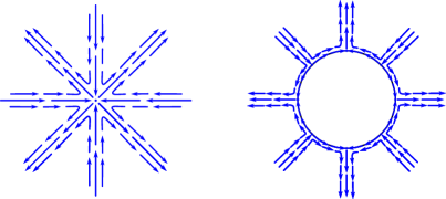
Figure 2.4.2: A $4$-pronged singularity on the left corresponding to the vector field $\bar{z}^{3}$. And a $4$-pronged boundary on the right.

If the surface $M$ has a boundary component $L$ such that after being contracted to a point, looks like a $k+1$-pronged singularity (see the right part of fig. 2.4.2), then

$$w_{\zeta}(L)=1+k$$

Similarly, for the vector field $\zeta=z^{k}$ on $\mathbb{C}$ with $k\geq 0$, we get a $k+1$-petal singularity (see fig. 2.4.3). By a similar computation the index in this case is

(2.4.9) $${\mathrm{Ind}}_{\zeta}(0)=k.$$

And, if $M$ has a boundary component $L$ such that after being contracted to a point, looks like a $k+1$-petal singularity, then

$$w_{\zeta}(L)=1-k$$

Figure 2.4.3: The vector field near the singularity of the vector field given by $z^{3}$: a $4$-petal singularity.

3 Embedded resolutions

In this section we explain several notions related to the resolutions of plane curve singularities, we also introduce notation and fix our conventions. We start by talking about different embedded resolutions and their dual graphs. We introduce the group of cycles associated with a modification and the notion of initial part and vanishing order of a function with respect to a variable or hypersurface. The latter two concepts play a central role in many of the subsequent proofs of this work.

After this, we introduce the maximal and canonical cycles which lead to the definition of two numerical invariants, $c_{0}$ and $c_{1}$, which allow us later to describe precisely the spine. We also include easy algorithms to compute them from the resolution process. For more details on the invariants and classical objects defined in these subsections, see [Ném99] or [Wal04].

In the last two subsections we introduce the structure of directed graph on the dual resolution graph $\Gamma$ and we introduce the notion of tangent associated with a divisor.

3.1 Embedded resolutions

Notation 3.1.1.

Let $(C,0)\subset(\mathbb{C}^{2},0)$ be an isolated plane curve singularity defined by a germ $f:(\mathbb{C}^{2},0)\to(\mathbb{C},0)$. Let $\pi:Y\to\mathbb{C}^{2}$ be an embedded resolution, that is, $\pi$ is a modification of $\mathbb{C}^{2}$ with $\pi^{-1}(0)$ a strict normal crossings divisor. Factorize $\pi$ as

(3.1.2) $$\pi=\pi_{0}\circ\pi_{1}\circ\cdots\circ\pi_{s}$$

where $\pi_{i}:(Y_{i},D_{i})\to(Y_{i-1},p_{i})$ are blow-ups. Set also $\bar{\pi}_{i}=\pi_{i}\circ\cdots\circ\pi_{0}:Y_{i}\to\mathbb{C}^{2}$. In particular, $\pi_{0}$ is the usual blow-up of $\mathbb{C}^{2}$ at the origin. We identify the divisors $D_{i}\in Y_{i}$ with their strict transforms in $Y_{j}$ for $j>i$. Set

$$D=\bigcup_{i=0}^{s}D_{i}\subset Y=Y_{s}.$$

Let $\tilde{C}$ be the strict transform of $C$ in $Y$.

Examples of embedded resolutions that appear in this work are

$$\pi_{\mathrm{min}}:(Y_{\mathrm{min}},D_{\mathrm{min}})\to(\mathbb{C}^{2},0)$$

which is the minimal embedded resolution. Similarly, we have

$$\pi_{\mathrm{pol}}:(Y_{\mathrm{pol}},D_{\mathrm{pol}})\to(\mathbb{C}^{2},0)$$

which is the minimal embedded resolution that also resolves the generic polar locus (cf. Subsection 5.1).

Notation 3.1.3.

Let $\Gamma$ be the dual graph associated with the resolution $Y\to\mathbb{C}^{2}$ and the function $f$. This graph has set of vertices $\mathcal{W}=\mathcal{V}\cup\mathcal{A}$ where $\mathcal{V}=\{0,1,\ldots,s\}$, and $\mathcal{A}$ is in bijection with the branches of $(C,0)$, where $(C,0)=\bigcup_{a\in\mathcal{A}}(C_{a},0)$. Then $i,j\in\mathcal{W}$ are joined by an edge $ij$ in $\Gamma$ if and only if $D_{i}\cap D_{j}\neq\emptyset$. Here, if $a\in\mathcal{A}$, we are denoting by $D_{a}$ as the strict transform of $C_{a}$ in $Y$. In this case, we denote by $p_{ij}$ the intersection point $D_{i}\cap D_{j}$.

Set $D_{\mathcal{V}}=D$, as well as $D_{\mathcal{A}}=\bigcup_{a\in\mathcal{A}}D_{a}$ and $D_{\mathcal{W}}=\bigcup_{w\in\mathcal{W}}D_{w}$. For $i\in\mathcal{W}$, set

$$D_{i}^{\circ}=D_{i}\setminus\bigcup_{j\in\mathcal{W}\setminus\{i\}}D_{j}.$$

Similarly we can define the graphs $\Gamma_{i}$ associated with the modifications $\bar{\pi}_{i}:Y_{i}\to\mathbb{C}^{2}$ for $i=0,1,\ldots,s$. These have a set of vertices $\mathcal{W}_{i}=\mathcal{V}_{i}\cup\mathcal{A}_{i}$. Furthermore, for each $j,k$ with $j<k$ there is a canonical injective map $\mathcal{V}_{j}\to\mathcal{V}_{k}$ and a bijective map $\mathcal{A}_{j}\to\mathcal{A}_{k}$.

The graphs $\Gamma$ and $\Gamma_{i}$ (for all $i$) are trees (see [Wal04, Section 3.6]). In particular, given two vertices $j,k\in\mathcal{W}$ or $\mathcal{W}_{i}$, there is a unique geodesic (path with the smallest number of edges possible) joining $j$ and $k$.

Next we recall the notion of group of cycles associated with a modification of $\mathbb{C}^{2}$.

Definition 3.1.4.

The group of cycles $L$ associated with the modification $Y\to\mathbb{C}^{2}$ is the free Abelian group generated by the exceptional divisors $D_{i}$ for $i\in\mathcal{V}$.

Remark 3.1.5.

Set $V=\pi^{-1}(B_{\varepsilon})$, where $B_{\varepsilon}$ is a Milnor ball. By, [Wal04, Lemma 8.1.1], the group of cycles is isomorphic to $H_{2}(V;\mathbb{Z})\cong H^{2}(V,\partial V;\mathbb{Z})$, that is, this homology group is freely generated by the homology classes of exceptional components $D_{i}$, $i\in\mathcal{V}$. Furthermore, since $\partial V\cong S^{3}$, the long exact sequence of the pair $(V,\partial V)$ induces an isomorphism

$$H_{2}(V;\mathbb{Z})\to H_{2}(V,\partial V;\mathbb{Z})\cong H^{2}(V;\mathbb{Z}).$$

As a result, with the identification $L=H_{2}(V,\mathbb{Z})$, Poincaré duality induces a unimodular pairing

$$(\cdot,\cdot):L\times L\to\mathbb{Z}.$$

Definition 3.1.6.

We define the antidual basis $D_{j}^{*}$, $j\in\mathcal{V}$ as the unique elements $D_{j}^{*}\in L$ satisfying $(D_{i},D_{j}^{*})=-\delta_{ij}$.

3.2 Initial part and vanishing order

Here we define several notions related to the order of vanishing of a real analytic function taking values in $\mathbb{C}$.

Definition 3.2.1.

Let $g:(\mathbb{C}^{2},0)\to(\mathbb{C},0)$ be a Laurent series in coordinates $u,v$ given by

$$g(u,v)=\sum_{i,j,k,l\in\mathbb{Z}}a_{ijkl}u^{i}v^{j}\bar{u}^{k}\bar{v}^{l}.$$

Let $\mathrm{ord}g=\min\left\{i+j+k+l\,\middle|\,a_{ijkl}\neq 0\right\}$. Then, we define the initial part of $g$ as

$$\mathop{\mathrm{in}}\nolimits g(u,v)=\sum_{i+j+k+l=\mathrm{ord}g}a_{ijkl}u^{i}v^{j}\bar{u}^{k}\bar{v}^{l}.$$

Definition 3.2.2.

Let $g:(\mathbb{C}^{2},0)\to(\mathbb{C},0)$ be a Laurent series in coordinates $u,v$ given by

$$g(u,v)=\sum_{i,j,k,l\in\mathbb{Z}}a_{ijkl}u^{i}v^{j}\bar{u}^{k}\bar{v}^{l}.$$

We define the vanishing order of $g$ with respect to $u$ as

$$\mathrm{ord}_{u}g=\min\left\{i+k\,\middle|\,a_{ijkl}\neq 0\right\}.$$

Then, we define the initial part of $g$ with respect to $u$ as the Laurent series given by

$$(\mathop{\mathrm{in}}\nolimits_{u}g)(u,v)=\sum_{i+k=\mathrm{ord}_{u}g}a_{ijkl}u^{i}v^{j}\bar{u}^{k}\bar{v}^{l}$$

Definition 3.2.3.

Let $h:(\mathbb{C}^{2},0)\to(\mathbb{C},0)$ be the germ of a real analytic function, and let $\pi:Y\to\mathbb{C}^{2}$ be as in Notation 3.1.1 and let $p\in D_{i}\subset Y$ with $i\in\mathcal{V}$. And let $U\subset Y$ a coordinate neighborhood around $p$ with coordinates $u,v$ so that $D_{i}\cap U$ is defined by $u=0$. We define the vanishing order of $h$ along $D_{i}$ by

$$\mathrm{ord}_{D_{i}}(h)=\mathrm{ord}_{u}(\pi^{*}h).$$

Remark 3.2.4.

Given a function $h:(\mathbb{C}^{2},0)\to(\mathbb{C},0)$ and a modification $\pi:Y\to\mathbb{C}^{2}$ with dual graph $\Gamma$, there is a cycle associated to $\pi^{*}h$ defined by

$$(\pi^{*}h)=\sum_{i\in\mathcal{V}}\mathrm{ord}_{D_{i}}(h)D_{i}.$$

In the antidual basis $D^{*}_{j}$, the cycle takes the form

$$(\pi^{*}h)=\sum_{i\in\mathcal{V}}a_{i}D^{*}_{i},$$

where $a_{i}$ is the multiplicity intersection of $D_{i}$ and the strict transform of $\{h=0\}$, that is, the number of intersection points of $D_{i}$ with a small perturbation of the strict transform of $\{h=0\}$. (See [Ném99]).

Definition 3.2.5.

For $i\in\mathcal{W}$, we set

$$m_{i}=\mathrm{ord}_{D_{i}}(f).$$

Note that, if $a\in\mathcal{A}$, then $m_{a}$ is the vanishing order of $f$ along one of the branches of $C$ (which might be bigger than $1$ if $f$ has non isolated critical points).

3.3 Invariants of the resolution: $c_{0},c_{1}$ and the canonical divisor

In this subsection, we introduce numerical invariants of the modification $Y\to\mathbb{C}^{2}$. In particular, these do not depend on $f$ or the metric $g$. All of this subsection is either part of the classical theory of plane curve singularities, or it may be deduced from [BdSFP22], (for example Lemma 3.3.7 is implied by [BdSFP22, Lemma 3.6]). However, since our setting is different and we need to fix notation, we briefly rework this theory.

Definition 3.3.1.

Denote by $Z_{\mathrm{max}}$ the maximal cycle in $Y$, and denote by $c_{0,i}$ its coefficients. Thus,

$$Z_{\mathrm{max}}=\sum_{i\in\mathcal{V}}c_{0,i}D_{i}.$$

and we have $c_{0,i}=\mathrm{ord}_{D_{i}}(\ell)$, where $\ell:\mathbb{C}^{2}\to\mathbb{C}$ is a generic linear function. Here generic means that the strict transform of $\{\ell=0\}$ intersects $D_{0}^{\circ}$, or equivalently, that $\{\ell=0\}$ is not a tangent of $C$ at the origin.

Since $c_{0,i}=\mathrm{ord}_{D_{i}}(\ell)$ we can similarly define these numbers for arrowheads, that is for $i\in\mathcal{A}$. In this case $c_{0,i}=\mathrm{ord}_{D_{i}}(\ell)=0$.

Remark 3.3.2.

We recall a basic fact about vanishing orders of linear functions (see for example [Ném99]). If $\ell$ is a generic linear function and $\ell^{\prime}$ is any other linear function then,

$$\mathrm{ord}_{D_{i}}(\ell^{\prime})\geq\mathrm{ord}_{D_{i}}(\ell)$$

for all $i\in\mathcal{V}$. We also have

$$c_{0,i}=\min\{\mathrm{ord}_{D_{i}}(x),\mathrm{ord}_{D_{i}}(y)\}$$

for $x,y$ any coordinate system in $\mathbb{C}^{2}$.

Definition 3.3.3.

Denote by $K$ the canonical cycle on $Y$ and by $\nu_{i}-1$ its coefficients. Thus,

$$K=\sum_{i\in\mathcal{V}}(\nu_{i}-1)D_{i}.$$

A canonical divisor on a smooth variety $X$ of dimension $d$ is defined as the divisor defined by any section of the canonical sheaf $\Omega_{X}^{d}$. The canonical cycle defined above is the unique canonical divisor supported on the exceptional set of $\pi$. In fact, for $d=2$ take the standard holomorphic two-form $dx\wedge dy\in\Omega_{\mathbb{C}^{2}}^{2}$ on $\mathbb{C}^{2}$. Then $K$ is the divisor defined by the section $\pi^{*}(dx\wedge dy)$ of $\Omega_{Y}^{2}$.

$K$ can be seen as a Cartier divisor as follows. If $U\subset Y$ is a coordinate chart, with coordinates $u,v$, we have a Jacobian matrix

$$\mathop{\mathrm{Jac}}\pi(u,v)=\left(\begin{matrix}\partial_{u}\pi^{*}x&\partial_{v}\pi^{*}x\\ \partial_{u}\pi^{*}y&\partial_{v}\pi^{*}y\end{matrix}\right).$$

The pairs $(U,\det\mathop{\mathrm{Jac}}\pi)$ constitute a Cartier divisor, whose associated Weil divisor is $K$.

Yet another characterization goes as follows. $K$ is the unique exceptional divisor satisfying the adjunction formulas:

$$(K,D_{i})=-D_{i}^{2}-2,\qquad i\in\mathcal{V}.$$

3.3.4.

Let $p\in D^{\circ}_{i}$ for some $i\in\mathcal{V}$, and choose a (small) coordinate neighborhood $U$ of $p$. Assume that $x,y$ are coordinates in $\mathbb{C}^{2}$, with $x$ a generic linear function. Then the function $\pi^{*}x$ vanishes with order $c_{0}=c_{0,i}$ along $D_{i}$, and does not vanish on $U\setminus D_{i}$. As a result, coordinates $u,v$ can be chosen for $U$ so that $\pi^{*}x=u^{c_{0}}$. Expand the second coordinate around $p\in U$ as

$$\pi^{*}y=\sum_{k\geq c_{0}}u^{k}g_{k}(v),$$

where $g_{k}$ are holomorphic functions defined in a neighborhood of $p$ in $D_{i}^{\circ}$ (possibly smaller than $U\cap D_{i}^{\circ}$). We are interested in the smallest number $k$ so that $g_{k}$ really depends on $v$, i.e. is not constant. Denote this number by $c_{1}$. The Jacobian of $\pi$ in these coordinates has a triangular form

(3.3.5) $$\left(\begin{matrix}\partial_{u}\pi^{*}x&\partial_{v}\pi^{*}x\\ \partial_{u}\pi^{*}y&\partial_{v}\pi^{*}y\end{matrix}\right)=\left(\begin{matrix}c_{0}u^{c_{0}-1}&0\\ \sum_{k}ku^{k-1}g_{k}(v)&\sum_{k}u^{k}g_{k}^{\prime}(v)\end{matrix}\right)$$

and so $c_{1}$ is the order of vanishing of $\partial_{v}\pi^{*}y$ along $D_{i}^{\circ}$. That is

$$\mathrm{ord}_{u}(\partial_{v}\pi^{*}y)=c_{1}.$$

Furthermore, we see that

$$\mathrm{ord}_{u}(\det\mathop{\mathrm{Jac}}\pi)=c_{0}+c_{1}-1.$$

But this order of vanishing is $\nu_{i}-1$ (recall Definition 3.3.3), which is independent of the choices we made so far. This motivates the following definition of the numbers $c_{1,i}$:

Definition 3.3.6.

For each vertex $i\in\mathcal{V}$, set

$$c_{1,i}=\nu_{i}-c_{0,i}.$$

As we did in Definition 3.3.1, just set $c_{1,i}=0$ for $i\in\mathcal{A}$.

Lemma 3.3.7.

Let $\pi_{i}:(Y_{i},D_{i})\to(Y_{i-1},p_{i})$ be the $i$-th blow up as in Notation 3.1.1. Then,

• If $i=0$, then

  $$c_{0,0}=c_{1,0}=1.$$

• If there is $j<i$, such that $p_{i}$ lies on a smooth point of the exceptional divisor $D_{j}$, that is $p_{i}\in D_{j}^{\circ}$, then

  $$c_{0,i}=c_{0,j},\qquad c_{1,i}=c_{1,j}+1.$$

• If there are $j,k<i$, such that $p_{i}$ lies at the intersection, $p_{i}\in D_{j}\cap D_{k}$, then

  $$c_{0,i}=c_{0,j}+c_{0,k},\qquad c_{1,i}=c_{1,j}+c_{1,k}.$$

Proof.

The first equality is a direct computation using the usual coordinates $\pi_{0}^{*}x=u,\pi_{0}^{*}y=uv$. The two formulas for $c_{0,i}$ follows immediately, since this is the vanishing of a generic linear function along the divisor $D_{i}$ (see the more general, [Wal04, Lemma 8.1.2]). The formula for $c_{1,i}$ follows, using the Definition 3.3.6, and the well known fact (see the proof of [Wal04, Proposition 8.1.8] that $\nu_{i}=\nu_{j}+1$ if $p_{i}$ is a smooth point, and $\nu_{i}=\nu_{j}+\nu_{k}$ if $p_{i}$ is an intersection point of two divisors. ∎

As a direct consequence of the recursive formulas provide, we have the following corollary.

Corollary 3.3.8.

For any $i\in\mathcal{V}$, we have $c_{1,i}\geq c_{0,i}$, with equality if and only if $i=0$.∎

The next important corollary yields a hierarchy on the set of vertices $\mathcal{V}$. We make explicit use of this hierarchy in the next subsection and throughout the rest of the paper.

Corollary 3.3.9.

If $i,j$ are neighbors in the resolution graph $\Gamma$, then we have a nonzero determinant

(3.3.10) $$\left|\begin{matrix}c_{0,i}&c_{1,i}\\ c_{0,j}&c_{1,j}\end{matrix}\right|\neq 0.$$

Furthermore, the above determinant is negative if and only if the geodesic (in $\Gamma$) from $0$ to $i$ passes through $j$.

Proof.

We use induction on $i=0,1,\ldots,s$. Assume the statement holds for $\Gamma_{i-1}$. We recall from Notation 3.1.3 that the set of vertices $\mathcal{V}_{i-1}$ of $\Gamma_{i-1}$ naturally embeds in the set of vertices $\mathcal{V}_{i}$ of $\Gamma_{i}$. Actually, there is a unique extra vertex $i\in\mathcal{V}_{i}$ that is not in $\mathcal{V}_{i-1}$. We treat two different cases depending on whether $p_{i}$ is a smooth point or an intersection point between two divisors (see also fig. 3.4.1).

Case 1. If $p_{i}$ lies on a smooth point of $D_{j}$, then there is a unique edge $ij$ in $\Gamma_{i}$ that is not in $\Gamma_{i-1}$. In this case $i$ is further from $0$ than $j$, and Lemma 3.3.7 gives

$$\left|\begin{matrix}c_{0,i}&c_{1,i}\\ c_{0,j}&c_{1,j}\end{matrix}\right|=c_{0,i}c_{1,j}-c_{1,i}c_{0,j}=c_{0,i}c_{1,j}-(c_{1,j}+1)c_{0,i}=-c_{0,i}<0.$$

Case 2. If $p_{i}$ is the intersection point $D_{j}\cap D_{k}$, then there are two edges $ik$ and $ij$ in $\Gamma_{i}$ that are not in $\Gamma_{i-1}$. In this case, Lemma 3.3.7 gives

$$\left|\begin{matrix}c_{0,i}&c_{1,i}\\ c_{0,j}&c_{1,j}\end{matrix}\right|=\left|\begin{matrix}c_{0,k}&c_{1,k}\\ c_{0,i}&c_{1,i}\end{matrix}\right|=\left|\begin{matrix}c_{0,k}&c_{1,k}\\ c_{0,j}&c_{1,j}\end{matrix}\right|$$

because

$$c_{0,i}=c_{0,j}+c_{0,k},\qquad c_{1,i}=c_{1,j}+c_{1,k}$$

and row operations preserve determinants. ∎

Corollary 3.3.11.

If $i\in\mathcal{V}$ is a neighbor of the vertex $0$, which corresponds to the first blow-up, then $c_{i,1}=c_{0,i}+1$. ∎

3.4 Directions on the dual graph

We endow $\Gamma$ with the structure of an directed graph and deduce some combinatorial properties of this structure in terms of $c_{0}$ and $c_{1}$.

Definition 3.4.1.

The graph $\Gamma$ is seen as a directed graph as follows. Let $i,j$ be neighbors in $\Gamma$. The edge $ij$ is directed from $j$ to $i$ if and only if the determinant eq. 3.3.10 is negative. In order to express that the edge $ij$ is oriented from $j$ to $i$ we write $j\to i$.

Similarly, the graphs $\Gamma_{i}$ corresponding to the modifications $\bar{\pi}_{i}:Y_{i}\to\mathbb{C}^{2}$ are directed for each $i=0,1,\ldots,s$ following the same criterion.

Figure 3.4.1: Effect of a blow-up on directed graphs. On top the effect of blowing up a smooth point at $D_{j}$. On bottom, the effect of blowing up the intersection point $D_{j}\cap D_{k}$.

Remark 3.4.2.

The orientations of the edges defined in Definition 3.4.1 are the same as the ones induced by the criterion:

“orient an edge $ij$ from $j$ to $i$ if $i$ is further from $0$ than $j$.”

Observe that each vertex $i\in\mathcal{V}$ with $i\neq 0$ has exactly one neighbor $j$ such that $j\to i$. This allows the following definition.

Definition 3.4.3.

Let $i$ be a vertex in the directed graph $\Gamma$, as above. If $i\neq 0$, let $j$ be the unique neighbor of $i$ such that $j\to i$. The branch (fig. 3.4.2) of $\Gamma$ at $i$ is

1. $\Gamma$, if $i=0$ and,

2. otherwise, the connected component of $\Gamma$ with the edge $ji$ removed, containing $i$.

Remark 3.4.4.

The branch of $\Gamma$ at $i$ is a tree rooted at $i$ (note that $i$ is the vertex which is the closest to $0$ among all vertices of the branch). Moreover, if $\Xi$ is a branch of $\Gamma$ at $i$ then, it satisfies that if $j\in\mathcal{W}_{\Xi}$ and $j\to k$, then $k\in\mathcal{W}_{\Xi}$.

Arrowheads in $\Gamma$ are included in the above definition. Thus, the branch at $i$ contains a subset of the arrowheads of $\Gamma$.

Figure 3.4.2: In red the branch at the vertex $i$ and in green the branch at the vertex $j$.

Lemma 3.4.5.

Let $i,j\in\mathcal{V}$, and assume that $\Gamma$ has an edge $j\to i$. If $g\in\mathcal{O}_{\mathbb{C}^{2},0}$, then

$$\det\left(\begin{matrix}c_{0,i}&\mathrm{ord}_{D_{i}}(g)\\ c_{0,j}&\mathrm{ord}_{D_{j}}(g)\end{matrix}\right)\leq 0.$$

If $\bar{\mathcal{V}}\subset\mathcal{V}$ is the set of vertices on the branch of $\Gamma$ at $i$, then equality holds if and only if the strict transform of the curve defined by $g=0$ does not intersect any $D_{k}$ for $k\in\bar{\mathcal{V}}$.

Proof.

In this proof, cycles are considered in the group $L\otimes\mathbb{Q}\simeq H(V;\mathbb{Q})$. Set $n_{k}=\mathrm{ord}_{D_{k}}(g)$ for $k\in\mathcal{V}$, and $Z=\sum_{k}n_{k}D_{k}\in L$. Thus, $Z$ is the cycle associated with $\pi^{*}g$. This cycle can be written in terms of the antidual basis as $Z=\sum_{k\in\mathcal{V}}a_{k}D_{k}^{*}$, with $a_{k}\geq 0$ (recall Remark 3.2.4).

Let $\bar{\Gamma}$ be the branch of $\Gamma$ at $i$, with vertex set $\bar{\mathcal{V}}\subset\mathcal{V}$. Since the intersection form is negative definite, there exist unique rational cycles $\bar{D}_{k}^{*}$ for $k\in\bar{\mathcal{V}}$ supported on $\bar{\Gamma}$ satisfying $(\bar{D}_{k}^{*},D_{l})=-\delta_{k,l}$ for $l\in\bar{\mathcal{V}}$, and furthermore, $\bar{D}_{k}^{*}$ has positive coefficients in the standard basis $\{D_{i}\}_{i\in\bar{\mathcal{V}}}$.

Define $\bar{Z}=\sum_{k\in\bar{\mathcal{V}}}a_{k}\bar{D}^{*}_{k}$. Then $\bar{Z}=\sum_{k\in\bar{\mathcal{V}}}\bar{n}_{k}D_{k}$, with nonnegative coefficients $\bar{n}_{k}\in\mathbb{Q}$. For $k\in\bar{\mathcal{V}}$, set $n_{k}^{\prime}=n_{k}-\bar{n}_{k}$ and $Z^{\prime}=\sum_{k\in\bar{\mathcal{V}}}n_{k}^{\prime}D_{k}$. Thus, $Z^{\prime}$ is supported on $\bar{\Gamma}$, and one verifies, for $k\in\bar{\mathcal{V}}$, $(Z^{\prime},D_{k})=-n_{j}\delta_{ik}$. As a result, $Z^{\prime}=n_{j}\bar{D}_{i}^{*}$.

In a similar way, if we set $\bar{Z}_{\mathrm{max}}=\sum_{k\in\bar{\mathcal{V}}}c_{0,k}D_{k}$, we have $(\bar{Z}_{\mathrm{max}},D_{k})=-c_{0,j}\delta_{ik}$, i.e. $\bar{Z}_{\mathrm{max}}=c_{0,j}\bar{D}^{*}_{i}=c_{0,j}/n_{j}Z^{\prime}$. As a result,

$$n_{i}=n_{i}^{\prime}+\bar{n}_{i}\geq n_{i}^{\prime}=\frac{n_{j}c_{0,i}}{c_{0,j}},$$

and so the determinant from the statement of this lemma equals $c_{0,i}n_{j}-c_{0,j}n_{i}\leq 0$. Furthermore, we have equality if and only if all the $a_{k}$ vanish for $k\in\bar{\mathcal{V}}$. But these coefficients are nothing but the intersection between the strict transform of the vanishing set of $g$ and $D_{k}$. ∎

Example 3.4.6.

We consider the case of a toric modification of $\mathbb{C}^{2}$, see [Ful93] for definitions used here. Let $\triangle$ be a regular subdivision of the positive quadrant. This gives a modification $\pi_{\triangle}:Y\to\mathbb{C}^{2}$, where $Y$ is smooth. An irreducible component of the exceptional divisor corresponds to a ray $\rho\in\triangle$ generated by a unique primitive vector $(a,b)\in\mathbb{Z}^{2}$ with $a,b>0$ and $\gcd(a,b)=1$. Call the component $D_{\rho}$. We can choose an adjacent ray $\theta$ generated similarly by $(c,d)$, so that $\eta=\rho+\theta$ is a two-dimensional cone in $\triangle$ and $ad-bc=1$. The affine toric variety $U_{\eta}\cong\mathbb{C}^{2}$ provides a coordinate neighborhood containing all but one point of $D_{\rho}$. Denoting by $u,v$ the coordinates in $D_{\eta}$, we have

$$\pi_{\triangle}(u,v)=(u^{a}v^{c},u^{b}v^{d}),\qquad U_{\eta}\cap D_{\rho}=\{u=0\}.$$

We therefore have $\mathrm{ord}_{D_{\rho}}x=a$, $\mathrm{ord}_{D_{\rho}}y=b$ and so $c_{0,\rho}=\min\{a,b\}$. Assuming that $a\leq b$, take a local coordinate change $\tilde{u}=uv^{a/c},\tilde{v}=v$. Then we have $x=\tilde{u}^{c_{0,\rho}}$, and $y=\tilde{u}^{b}\tilde{v}^{d-bc/a}$. It follows that $c_{1,\rho}=b=\max\{a,b\}$.

3.5 The tangent associated with a divisor

We associate a tangent to each connected component of $\Gamma\setminus\{0\}$ and prove an easy, but useful, inequality of vanishing orders of linear functions.

Definition 3.5.1.

Setting $\pi^{\prime}=\pi_{1}\circ\cdots\circ\pi_{s}$, we have a factorization $\pi=\pi_{0}\circ\pi^{\prime}$. For $p\in D\subset Y$, we define the tangent associated with $p$ as the line in $\mathbb{C}^{2}$ corresponding to the point $\pi^{\prime}(p)\in D_{0}\subset Y_{0}$. If $i\neq 0$, then the tangent associated with $p\in D_{i}$ is independent of $p$. So whenever $i\neq 0$, we also speak of the tangent associated with $D_{i}$.

The following lemma expresses the idea that tangents are precisely the non-generic complex lines relative to a given plane curve.

Lemma 3.5.2.

Let $i\in\mathcal{V}\setminus\{0\}$, and let $x,y$ be linear coordinates in $\mathbb{C}^{2}$ such that $\{y=0\}$ is the tangent associated with $D_{i}$. Then

$$\mathrm{ord}_{D_{i}}(y)>\mathrm{ord}_{D_{i}}(x)=c_{0,i}.$$

Proof.

Since $\{x=0\}$ is not the tangent associated with $D_{i}$, the vanishing order of $\pi^{*}x$ along $D_{i}$ is that of a generic linear function which is, by definition (recall Definition 3.3.1) $c_{0,i}$. In particular, since $y$ is another linear function, by Remark 3.3.2 we have the inequality

$$\mathrm{ord}_{D_{i}}(y)\geq\mathrm{ord}_{D_{i}}(x).$$

The fact that $\{y=0\}$ is the tangent associated to $D_{i}$ implies that its strict transform by the first blow up $\pi_{0}$ does not pass through $D_{0}^{\circ}$ (it has to pass through one of the intersection,, let’s say $p$ points of the strict transform of $C$ by $\pi_{0}$). Since we are assuming that $i\neq 0$, we know that the resolution $\pi=\pi_{0}\circ\pi_{1}\circ\cdots\circ\pi_{s}$ includes the blow up at $p\in D_{0}$. Let $\pi_{k}:Y_{k}\to Y_{k-1}$ be the blow up at $p$. Then $\mathrm{ord}_{D_{k}}(x)=1$ and $\mathrm{ord}_{D_{k}}(y)=2$. Necessarily $i\geq k$ and after each new blow up, the order of vanishing of $y$ increases at least as that of $x$. This settles the strict inequality. ∎

4 The real oriented blow-up

In this section, we recall the definition of the real oriented blow-up of an embedded resolution along the exceptional set. This construction has been used before by other authors, see for example [A’C75] or, in a more general setting, [KN99].

Let $(Y,D)\to(\mathbb{C}^{2},0)$ be a modification of the origin as above (Notation 3.1.1). Denote by $\sigma_{i}:Y^{\mathrm{ro}}_{i}\to Y$ the real oriented blow-up of $Y$ along the submanifold $D_{i}\subset Y$ for $i\in\mathcal{W}$ constructed as follows. If $U\subset Y$ is a chart with coordinates $u,v$ such that $u=0$ is an equation for $D_{i}\cap U$, then we take a coordinate chart $U^{\mathrm{ro}}\subset Y^{\mathrm{ro}}_{i}$ with coordinates $r,\alpha,v\in\mathbb{R}_{\geq 0}\times\mathbb{R}/2\pi\mathbb{Z}\times\mathbb{C}$, where $r$ and $\alpha$ are polar coordinates for $u$, that is:

(4.0.1) $$r=|u|:U^{\mathrm{ro}}\to\mathbb{R},\qquad\alpha=\arg(u):U^{\mathrm{ro}}\to\mathbb{R}/2\pi\mathbb{Z}.$$

We can cover $D_{i}$ by such charts in order to define an atlas for $Y^{\mathrm{ro}}_{i}$. In each of these charts, the map $\sigma_{i}$ is given by $\sigma_{i}(r,\theta,v)=(re^{i\theta},v)$. Denote the fiber product of these maps by

(4.0.2) $$\sigma=\bigtimes_{i\in\mathcal{W}}\sigma_{i}:(Y^{\mathrm{ro}},D^{\mathrm{ro}}_{\mathcal{W}})\to(Y,D_{\mathcal{W}}).$$

The spaces $Y^{\mathrm{ro}}_{i}$ are manifolds with boundary, and the space $Y^{\mathrm{ro}}$ is a manifold with corners and, as a topological manifold, its boundary $\partial Y^{\mathrm{ro}}$ coincides with $D^{\mathrm{ro}}_{\mathcal{W}}$. Denote by $\pi^{\mathrm{ro}}$ the composition

$$\pi^{\mathrm{ro}}=\pi\circ\sigma:Y^{\mathrm{ro}}\to{\mathrm{Tub}}.$$

Similarly, we can consider the real oriented blow up of $\mathbb{C}$ at the origin

$$\sigma^{\prime}:\mathbb{C}^{\mathrm{ro}}\to\mathbb{C}.$$

In this case, $\mathbb{C}^{\mathrm{ro}}\simeq\mathbb{R}_{\geq 0}\times\mathbb{R}/2\pi\mathbb{Z}$ and $\sigma^{\prime}(r,\theta)=re^{2\pi i\theta}.$ The real-oriented blow up construction is functorial, that is, there exists a well defined map $f^{\mathrm{ro}}:Y^{\mathrm{ro}}\to\mathbb{C}^{\mathrm{ro}}$ that makes the diagram in eq. 4.0.3 commutative. We also say that the map $\sigma$ resolves the indeterminacy locus of the function $\arg(f)$ which results in a well defined function

$$\arg(f^{\mathrm{ro}})=\arg\circ f^{\mathrm{ro}}:Y^{\mathrm{ro}}\to\mathbb{R}/2\pi\mathbb{Z}.$$

We fit all this information in the following commutative diagram:

(4.0.3)

Notation 4.0.4.

The corners of $Y^{\mathrm{ro}}$ induce a stratification indexed by the graph $\Gamma$ as follows. Set $D^{\mathrm{ro}}_{\emptyset}=Y^{\mathrm{ro}}\setminus D^{\mathrm{ro}}_{\mathcal{W}}$. For $i,j\in\mathcal{W}$, we define the following subspaces of $\partial Y^{\mathrm{ro}}$:

$$D^{\mathrm{ro},\circ}_{i}=\sigma^{-1}(D_{i}^{\circ}),\qquad D^{\mathrm{ro}}_{i}=\sigma^{-1}(D_{i}),\qquad D^{\mathrm{ro}}_{i,j}=\sigma^{-1}(D_{i}\cap D_{j}).$$

Note that $\sigma^{-1}(D_{i})=\overline{D^{\mathrm{ro},\circ}_{i}}$.

4.1 An action on the normal bundle

For an $i\in\mathcal{W}$, the elements of $\sigma_{i}^{-1}(D_{i})=\partial Y^{\mathrm{ro}}_{i}$ correspond to oriented real lines in the normal bundle of $D_{i}\subset Y$, which has a complex structure. This induces a $\mathbb{C}^{*}$-action on $\partial Y^{\mathrm{ro}}_{i}$, with stabilizer $\mathbb{R}_{>0}\subset\mathbb{C}^{*}$, which reduces to a principal action of $\mathbb{R}/2\pi\mathbb{Z}\cong\mathbb{C}^{*}/\mathbb{R}_{>0}$. In particular, $D^{\mathrm{ro},\circ}_{i}$ is naturally a principal $S^{1}$-bundle over $D_{i}^{\circ}$, and $D^{\mathrm{ro}}_{i,j}\cong S^{1}\times S^{1}$. Denote this action by $\cdot_{i}$. In the coordinates $r,\alpha,v$ on $U^{\mathrm{ro}}$ introduced before in Section 4, this action is given by

$$\eta\cdot_{i}(0,\alpha,v)=(0,\alpha+\eta,v),\qquad\eta\in\mathbb{R}/2\pi\mathbb{Z}.$$

for a point $(0,\alpha,v)\in\partial U^{\mathrm{ro}}$.

Let $p\in D_{i}\cap D_{j}$ be an intersection point, and $U\ni p$ a coordinate chart with $U\cap D_{i}=\{u=0\}$ and $U\cap D_{j}=\{v=0\}$. We have polar coordinates $(r,s,\alpha,\beta)$ on $\sigma^{-1}(U)=U^{\mathrm{ro}}$ so that $\sigma(r,s,\alpha,\beta)=(re^{i\alpha},se^{i\beta})$. The corner

$$\sigma^{-1}(p)=\left\{(r,s,\alpha,\beta)\in U^{\mathrm{ro}}\,\middle|\,r=s=0\right\}$$

has two $\mathbb{R}/2\pi\mathbb{Z}$-actions. For $\eta,\nu\in\mathbb{R}/2\pi\mathbb{Z}$

$$\eta\cdot_{i}\nu\cdot_{j}(0,0,\alpha,\beta)=(0,0,\alpha+\eta,\beta+\nu).$$

Thus, the torus $\sigma^{-1}(p)$ is an $\mathbb{R}/2\pi\mathbb{Z}\times\mathbb{R}/2\pi\mathbb{Z}$-torsor.

Definition 4.1.1.

Let $U\subset Y$ and $U^{\mathrm{ro}}=\sigma^{-1}(U)$. A function $f:U^{\mathrm{ro}}\to\mathbb{C}$ is $\cdot_{i}$-equivariant of weight $k\in\mathbb{Z}$ if for all $p\in D^{\mathrm{ro}}_{i}\cap U^{\mathrm{ro}}$ and $\eta\in\mathbb{R}/2\pi\mathbb{Z}$, we have $f(\eta\cdot_{i}p)=e^{ik\eta}f(p)$. A function which is equivariant of weight $0$, is said to be invariant.

Lemma 4.1.2.

If $U\subset Y$ is open, and $h:U\to\mathbb{C}$ is a meromorphic function which is holomorphic on $U\setminus D_{i}$ and has vanishing order $k\in\mathbb{Z}$ along $D_{i}\cap U$. Then the pull-back $r^{-k}\sigma^{*}h$ of $|u|^{-k}h$ by $\sigma$, extends over the boundary to a real analytic equivariant function of weight $k$.

Similarly, the pull-back of $|u|^{-k}\bar{h}$ extends over the boundary to a real analytic equivariant function of weight $-k$.

Proof.

Since the statement of the lemma is local, we can assume that $U$ is a small coordinate chart around some $p\in D_{i}$, with coordinates $u,v$ so that the set $U\cap D_{i}$ is defined by $u=0$. Expand $h=\sum_{j=k}^{\infty}a_{j}(v)u^{j}$, where $a_{i}$ are holomorphic functions in the variable $v$. Then, using polar coordinates as in eq. 4.0.1,

$$r^{-k}\sigma^{*}h(r,\alpha,v)=\sum_{j=k}^{\infty}r^{-k+j}a_{k}(v)e^{ij\alpha}$$

which shows that $r^{-k}\sigma^{*}h$ is real analytic function which is well defined on all $U^{\mathrm{ro}}$. Restricting to the boundary, that is $r=0$, we get:

$$\left.(r^{-k}\sigma^{*}h)\right|_{r=0}=a_{k}(v)e^{ki\alpha}$$

and the first statement follows. The second statement is completely analogous. ∎

4.2 Milnor fibration at radius zero

In this subsection we introduce the Milnor fibration at radius zero, which is the fibration given by the map

$$\arg(f^{\mathrm{ro}})|_{\partial Y^{\mathrm{ro}}}:\partial Y^{\mathrm{ro}}\to\mathbb{R}/2\pi\mathbb{Z}.$$

Definition 4.2.1.

For $\theta\in\mathbb{R}/2\pi\mathbb{Z}$, we define the Milnor ray at angle $\theta$, as

$${\mathrm{Tub}}^{*}_{\theta}=\arg(f)^{-1}(\theta)\subset{\mathrm{Tub}}^{*},$$

as well as the subsets of $Y^{\mathrm{ro}}$:

(4.2.2) $$Y^{\mathrm{ro}}_{\theta} =\arg(f^{\mathrm{ro}})^{-1}(\theta),\qquad D^{\mathrm{ro}}_{i,\theta} =Y^{\mathrm{ro}}_{\theta}\cap D^{\mathrm{ro}}_{i},$$

$$D^{\mathrm{ro},\circ}_{i,\theta} =Y^{\mathrm{ro}}_{\theta}\cap D^{\mathrm{ro},\circ}_{i}, D^{\mathrm{ro}}_{i,j,\theta} =Y^{\mathrm{ro}}_{\theta}\cap D^{\mathrm{ro}}_{i,j}.$$

Remark 4.2.3.

In this remark we give a description of the fiber product of eq. 4.0.2 and introduce some notation that will be useful later on Subsection 12.2.

Let $i\in\mathcal{V}_{\Gamma}$. Let $\sigma_{i}$ be the real oriented blow up of $Y$ along $D_{i}$ . Denote $\tilde{D}^{\mathrm{ro}}_{i}=\sigma_{i}^{-1}(D_{i})\subset Y^{\mathrm{ro}}_{i}$. The real oriented blow up of $Y$ along $D_{i}$ resolves partially the indeterminacy of $\arg(f)$ and gives a well defined function

$$\arg_{i}(f):Y^{\mathrm{ro}}_{i}\setminus\left(\sigma_{i}^{-1}(D\setminus D_{i})\right)\to\mathbb{R}/2\pi\mathbb{Z}.$$

By definition of fiber product, there exists a map

$$\iota_{i}:Y^{\mathrm{ro}}\to Y^{\mathrm{ro}}_{i}$$

such that $\sigma_{i}\circ\iota_{i}=\sigma$ and $\iota_{i}|_{D^{\mathrm{ro}}_{i}}:D^{\mathrm{ro}}_{i}\to\tilde{D}^{\mathrm{ro}}_{i}$ is an isomorphism. This identification, lets us define

$$\tilde{D}^{\mathrm{ro}}_{i,\theta}=\iota_{i}(D^{\mathrm{ro}}_{i,\theta})$$

The space $Y^{\mathrm{ro}}$ is constructed, by definition, by considering the equivalence relation $\sim$ on $\bigsqcup_{k\in\mathcal{V}_{\Gamma}}Y^{\mathrm{ro}}_{k}$ given by $p\sim q$ if and only if

1. $p\in D^{\mathrm{ro},\circ}_{i}$ and $q\in D^{\mathrm{ro},\circ}_{j}$ and $ij$ is an edge of $\Gamma$

2. $\arg_{i}(f)(p)=\arg_{j}(f)(q)$

Lemma 4.2.4.

For any $\theta\in\mathbb{R}/2\pi\mathbb{Z}$, the set $Y^{\mathrm{ro}}_{\theta}$ is a submanifold of $Y$ which intersects the boundary strata transversely.

Proof.

It suffices to show that for every stratum $S\subset Y^{\mathrm{ro}}$, the restriction

$$\arg(f^{\mathrm{ro}})|_{S}:S\to\mathbb{R}/2\pi\mathbb{Z}$$

is a submersion. For $S=D^{\mathrm{ro}}_{\emptyset}$, this follows from the chain rule, and the fact that if $p\in Y^{\mathrm{ro}}\setminus D^{\mathrm{ro}}_{\mathcal{W}}\cong{\mathrm{Tub}}\setminus C$, then

$$D((\pi^{\mathrm{ro}})^{*}f)_{p}:TY_{p}\to T\mathbb{C}_{f(p)}$$

is a non-zero complex linear map, in particular, it is surjective.

Now take $p\in S=D^{\mathrm{ro},\circ}_{i}$ and let $U^{\mathrm{ro}}$ be a chart around $p$ with coordinates $r,\alpha,v$ and such that $D^{\mathrm{ro},\circ}_{i}\cap U^{\mathrm{ro}}$ is defined by $r=0$. The function $f$ in the chart $U^{\mathrm{ro}}$ takes the form

$$f=r^{m_{i}}e^{im_{i}\alpha}\tilde{f}$$

with $\tilde{f}$ a unit on $U^{\mathrm{ro}}$. Now, the function $f^{\mathrm{ro}}$ (recall eq. 4.0.3), in these coordinates, looks like

$$f^{\mathrm{ro}}(r,\alpha,v)=(r^{m_{i}}|\tilde{f}|,m_{i}\alpha+\arg(\tilde{f}))\in\mathbb{R}_{\geq 0}\times\mathbb{R}/2\pi\mathbb{Z}.$$

Now, we can compute

$$\arg(f^{\mathrm{ro}})(r,\alpha,v)=m_{i}\alpha+\arg(\tilde{f})$$

which, restricted to $S$, takes the form

$$\arg(f^{\mathrm{ro}})|_{S}(\alpha,v)=m_{i}\alpha+\arg(\tilde{f}).$$

Since $\partial_{\alpha}(\arg(f^{\mathrm{ro}})|_{S})=m_{i}\neq 0$, because $\arg(\tilde{f})$ does not depend on $\alpha$, we get again that $\arg(f^{\mathrm{ro}})|_{S}$ is a submersion.

A similar argument applies to $D^{\mathrm{ro}}_{i,j}$. ∎

As a consequence of Lemma 4.2.4 the map

$$\arg(f^{\mathrm{ro}})|_{\partial Y^{\mathrm{ro}}}:\partial Y^{\mathrm{ro}}\to\mathbb{R}/2\pi\mathbb{Z}$$

is a locally trivial topological fibration which is smooth when restricted to each of the strata (Notation 4.0.4) of $\partial Y^{\mathrm{ro}}$. Moreover, it is equivalent as a $C^{0}$-fibration to the Milnor fibration.

Definition 4.2.5.

The locally trivial fibration induced by $\arg(f^{\mathrm{ro}})|_{\partial Y^{\mathrm{ro}}}$ is called the Milnor fibration at radius $0$. We call its fiber $F^{\mathrm{ro}}_{\theta}=\arg(f^{\mathrm{ro}})|_{\partial Y^{\mathrm{ro}}}^{-1}(\theta)$ the Milnor fiber at radius $0$ over the angle $\theta$.

Remark 4.2.6.

Note that $F^{\mathrm{ro}}_{\theta}$ is a stratified manifold and that, for each $\theta\in\mathbb{R}/2\pi\mathbb{Z}$ it has a natural partition induced by the stratification of the exceptional set $D$:

$$F^{\mathrm{ro}}_{\theta}=\bigsqcup_{i\in\mathcal{W}}D^{\mathrm{ro},\circ}_{i,\theta}\bigsqcup_{\begin{subarray}{c}i,j\in\mathcal{W}\\ D_{i}\cap D_{j}\neq\emptyset\end{subarray}}D^{\mathrm{ro}}_{i,j,\theta}.$$

4.3 Scaling and extending the metric

In this subsection we explain how the pullback metric on $Y^{\mathrm{ro}}$ induces a metric on $D^{\mathrm{ro},\circ}_{i,\theta}$ for each $i\in\mathcal{V}\setminus\{0\}$ and each $\theta\in\mathbb{R}/2\pi\mathbb{Z}$.

Fix a vertex $i\in\mathcal{V}\setminus\{0\}$ and a value $\theta\in\mathbb{R}/2\pi\mathbb{Z}$. The set $D^{\mathrm{ro},\circ}_{i,\theta}$ covers the Riemann surface $D^{\circ}_{i}$, and so is a Riemann surface. Choose isometric coordinates (Definition 2.3.1), $x,y$ so that $\{y=0\}$ is the tangent associated with $D_{i}$. Let $U$ be a small coordinate chart of some point as in 3.3.4, with coordinates $u,v$ chosen so that the pullback $\pi^{*}x=u^{c_{0,i}}$, and in particular ${u=0}$ defines $D_{i}\cap U$. Recall that by Lemma 3.5.2, $\pi^{*}y$ vanishes with strictly higher order along $D_{i}$ than $\pi^{*}x$. By abuse of notation, we write $x$ rather than $\pi^{*}x$, and denote its partials with respect to $u$ and $v$ by $x_{u}$ and $x_{v}$, and so forth. With these assumptions, we have $x_{v}=0$. Denote by $\mathop{\mathrm{Jac}}\pi$ the Jacobian matrix eq. 3.3.5. Then, outside of the exceptional divisor, the pullback of the standard Hermitian metric in $\mathbb{C}^{2}$ is given by the Hermitian matrix

$$\mathop{\mathrm{Jac}}\pi^{*}\cdot\mathop{\mathrm{Jac}}\pi=\left(\begin{matrix}\bar{x}_{u}&\bar{y}_{u}\\ 0&\bar{y}_{v}\end{matrix}\right)\left(\begin{matrix}x_{u}&0\\ y_{u}&y_{v}\end{matrix}\right)=\left(\begin{matrix}|x_{u}|^{2}+|y_{u}|^{2}&\bar{y}_{u}y_{v}\\ \bar{y}_{v}y_{u}&|y_{v}|^{2}\end{matrix}\right)\in\mathop{\rm Mat}\nolimits(2\times 2,\mathbb{C})$$

which does not extend to give a Hermitian metric on all of $U$. However, the lower diagonal $|y_{v}|^{2}$ entry vanishes with order precisely $2c_{1,i}$. Thus, if we scale the metric by the function $|u|^{-2c_{1,i}}=|x|^{-2c_{1,i}/c_{0,i}}$, this lower diagonal entry gives a real $2\times 2$ matrix which is diagonal, and whose diagonal entries are the restriction to $U\cap D_{i}$ of the extension of $|y_{v}|^{2}/|u|^{2c_{1,i}}$ over $U\cap D_{i}$. Denote this function by $h_{U}$. Thus, if $(0,v)\in D_{i}\cap U$, then

$$h_{U}(v)=\lim_{u\to 0}\frac{|y_{v}|^{2}}{|u|^{2c_{1,i}}}.$$

Since this construction was made by scaling the pullback of the standard metric by the function $|x|^{-2c_{1,i}/c_{0,i}}=|u|^{-2c_{1,i}}$, this gives a metric of the whole set $D^{\circ}_{i}$, which in the coordinate neighborhood $U\cap D^{\circ}_{i}$ is given by the real $2\times 2$ matrix

$$\left(\begin{matrix}h_{U}&0\\ 0&h_{U}\end{matrix}\right)\in\mathop{\rm Mat}\nolimits(2\times 2,\mathbb{R})$$

In fact, one may verify that if $U^{\prime}$ is another coordinate neighborhood, then the above matrices define the same metric on the intersection. Since $D^{\mathrm{ro},\circ}_{i,\theta}$ covers $D^{\circ}_{i}$, the Riemann surface $D^{\mathrm{ro},\circ}_{i,\theta}$ inherits a Riemannian metric.

Definition 4.3.1.

Denote by $g_{i}$ and $g^{\mathrm{ro}}_{i,\theta}$ the Riemannian metrics on $D_{i}^{\circ}$ and $D^{\mathrm{ro},\circ}_{i,\theta}$ constructed above.

Remark 4.3.2.

A holomorphic coordinate $v$ in a chart $U\cap D_{i}^{\circ}$, as above, induces a trivialization of the tangent and cotangent bundles of $U\cap D_{i}^{\circ}$, which identifies a vector field or a one form with a complex function. Write $v=s+it$, so that $s,t$ are real coordinates. A vector field $\zeta=a\partial_{s}+b\partial_{t}$ on $U\cap D_{i}^{\circ}$ corresponds to the complex function $a+ib$, and a differential form $\eta=\alpha ds+\beta dt$ corresponds to the function $\alpha+i\beta$.

The form $\eta$ is dual to the vector field $\zeta$ with respect to the metric $g_{i}$, that is, $\eta=g_{i}(\zeta,\cdot)$ if and only if

$$\alpha+i\beta=h_{U}\cdot(a+ib).$$

If $\phi$ is a real function on $D^{\circ}_{i}\cap U$, then the gradient of $\phi$ with respect to the metric $g_{i}$ is given by

$$\nabla\phi=h_{U}^{-1}\cdot(\phi_{s}\partial_{s}+\phi_{t}\partial_{t}).$$

5 Resolving the polar locus

In this section we specify a genericity condition for the metric that involves the relative polar curves of the plane curve singularity. Before doing so, we review part of the needed theory.

5.1 Generic polar curves

In this subsection, we fix notation regarding relative polar curves and recall a result from Tessier that says that there is an equisingular family of relative polar curves which is dense among all polar curves.

Let $w=(w_{1},w_{2})\in\mathbb{C}^{2}\setminus\{0\}$ be a vector. By the canonical isomorphism $T_{p}\mathbb{C}^{2}\cong\mathbb{C}^{2}$ for any $p\in\mathbb{C}^{2}$, we identify $w$ with a vector field $\partial_{w}$ on $\mathbb{C}^{2}$. We denote the corresponding partial $\partial_{w}f$ of $f$ by $f_{w}$.

Definition 5.1.1.

The function $f_{w}:\mathbb{C}^{2}\to\mathbb{C}$ defines a plane curve. We denote this plane curve by

$$P_{w}=\{f_{w}=0\}.$$

That is, $P_{w}$ is the vanishing set of $f_{w}$. We call $P_{w}$ the relative polar curve of $f$ associated with $w$.

Observe that $P_{w}=P_{\lambda w}$ for any $\lambda\in\mathbb{C}^{*}$, and so $P_{w}$ only depends on the equivalence class $[w]\in\mathbb{CP}^{1}$. Denote the strict transform of $P_{w}$ in a modification $Y$ of $\mathbb{C}^{2}$ by $\tilde{P}_{w}$.

By [Tei77, pg. 269-270, Théorèm 2.], the family $P_{w}$ for $[w]\in\mathbb{CP}^{1}$ is equisingular on a Zariski open dense subset $\Omega$ of $\mathbb{CP}^{1}$. More concretely, here exist a modification

$$\pi:Y\to\mathbb{C}^{2}$$

as in eq. 3.1.2 and a set $\Omega\subset\mathbb{CP}^{1}$ satisfying the properties

1. if $[w]\in\Omega$, then $D\cup\tilde{X}\cup\tilde{P}_{w}$ is a normal crossing divisor. That is, $\pi$ is an embedded resolution for each $P_{w}$ with $w\in\Omega$,

2. if $[w],[w^{\prime}]\in\Omega$ and $i\in\mathcal{V}$, then the strict transforms of both associated polar curves $\tilde{P}_{w}$ and $\tilde{P}_{w^{\prime}}$ intersect the same number of points each divisor, that is $|D_{i}\cap\tilde{P}_{w}|=|D_{i}\cap\tilde{P}_{w^{\prime}}|$. Equivalently,

   $$\mathrm{ord}_{D_{i}}\pi^{*}f_{w}=\mathrm{ord}_{D_{i}}\pi^{*}f_{w^{\prime}}.$$

   Or, equivalently, the cycles associated with $\pi^{*}f_{w}$ and $\pi^{*}f_{w^{\prime}}$ coincide (recall Remark 3.2.4). We put a name to this cycle below.

3. $\Omega$ does not contain any of the tangents to $(C,0)$.

Definition 5.1.2.

We denote by $\pi_{\mathrm{pol}}:(Y_{\mathrm{pol}},D_{\mathrm{pol}})\to(\mathbb{C}^{2},0)$ the minimal embedded resolution of $(C,0)$ satisfying the above properties, and by $\Omega\in\mathbb{CP}^{1}$ the corresponding open set. Denote by $\Gamma_{\mathrm{pol}}$ its resolution graph, with $\mathcal{V}_{\mathrm{pol}}$ the set of vertices corresponding to exceptional components. Denote by $C_{\mathrm{pol}}$ and $P_{\mathrm{pol}}$ the strict transform of the curve $C$ and a polar curve $P_{w}$ for a $w\in\Omega$, respectively.

Remark 5.1.3.

1. Observe that $\pi_{\mathrm{pol}}$ can be obtained from $\pi_{\mathrm{min}}$ by iteratively blowing map at intersection points of $P_{\mathrm{min}}$ with the exceptional set.

2. Any embedded resolution $\pi:Y\to\mathbb{C}^{2}$ that resolves the Jacobian ideal $J=(f_{x},f_{y})$, i.e. such that $\pi^{*}J$ is principal, satisfies properties items (i), (ii) and (iii) above.

Property item (ii) above leads to the following definition:

Definition 5.1.4.

For $[w]\in\Omega$ and $i\in\mathcal{V}_{\mathrm{pol}}$, define a cycle $Z_{P}\in L$ (in the group of cycles associated with the modification $\pi_{\mathrm{pol}}$) and integers $p_{i}$ for $i\in\mathcal{V}$ by

$$Z_{P}=\sum_{i\in\mathcal{V}}|P_{\mathrm{pol}}\cap D_{i}|D^{*}_{i}=\sum_{i\in\mathcal{V}}p_{i}D_{i}.$$

For $a\in\mathcal{A}$ we define $p_{a}=\mathrm{ord}_{D_{a}}f_{w}=m_{a}-1$.

Remark 5.1.5.

Recall that by Remark 3.2.4, $\mathrm{ord}_{D_{i}}(f_{w})=p_{i}$. An equivalent definition of the numbers $p_{i}$, which does not depend on any choice, is

(5.1.6) $$p_{i}=\min\{\mathrm{ord}_{D_{i}}(f_{x}),\;\mathrm{ord}_{D_{i}}(f_{y})\}.$$

This is because a relative polar curve is defined by taking a linear combination of the partials $f_{x}$ and $f_{y}$.

The next lemma shows that the number of intersection points of a generic polar curve with the first divisor is controlled by the number of tangents of the plane curve.

Lemma 5.1.7.

For $w\in\Omega$, the number of intersection points of the divisor $D_{0}$ corresponding to the first blow-up and $P_{\mathrm{pol}}$ is $|D_{0}\cap P_{\mathrm{pol}}|=t-1$, where $t$ is the number of different tangents of $(C,0)$.

Proof.

Let $e$ be the multiplicity of $(C,0)$ so that $f=\mathop{\mathrm{in}}\nolimits(f)+\cdots$ where $\mathop{\mathrm{in}}\nolimits(f)$ is a homogeneous polynomial of degree $e$, and $\cdots$ stands for higher order terms. Distinct linear factors of $\mathop{\mathrm{in}}\nolimits(f)$ correspond to tangents of $(C,0)$. Therefore, we have distinct points $[a_{i},b_{i}]\in\mathbb{CP}^{1}$, and positive integers $e_{i}$ so that $e_{1}+\ldots+e_{t}=e$ and

$$\mathop{\mathrm{in}}\nolimits(f)(x,y)=\prod_{i=1}^{t}(a_{i}x-b_{i}y)^{e_{i}}$$

We can assume $w=(0,1)$ up to a change of coordinates. In this case $f_{w}=f_{y}$. Then the intersection points $D_{0}\cap P_{\mathrm{pol}}$ correspond to the roots of the homogeneous polynomial $\mathop{\mathrm{in}}\nolimits(f)_{y}$, which are not roots of $\mathop{\mathrm{in}}\nolimits(f)$. Note that $\mathop{\mathrm{in}}\nolimits(f_{y})=\mathop{\mathrm{in}}\nolimits(f)_{y}$, because, since $y$ is not a tangent, $\mathop{\mathrm{in}}\nolimits(f)$ has the monomial $y^{e}$ with nonzero coefficient. As a result, $\mathop{\mathrm{in}}\nolimits(f_{y})$ is a homogeneous polynomial of degree $e-1$, and has a root of multiplicity $(e_{i}-1)$ at $[a_{i},b_{i}]$.

To finish the proof, it is enough to show that the Jacobian ideal has no base point on $D_{0}$ outside the strict transform of $C$ in $Y_{0}$. In other words, it suffices to show that $\mathop{\mathrm{in}}\nolimits f_{x}$ and $\mathop{\mathrm{in}}\nolimits f_{y}$ have no common factors other than the roots of $\mathop{\mathrm{in}}\nolimits(f)$. But a common root of $\mathop{\mathrm{in}}\nolimits f_{x},\mathop{\mathrm{in}}\nolimits f_{y}$ is a root of $\mathop{\mathrm{in}}\nolimits f$ by Euler’s identity $xf_{x}+yf_{y}=ef$. ∎

Remark 5.1.8.

In the above proof, we have seen that the Jacobian ideal $(f_{x},f_{y})\subset\mathcal{O}_{C,0}$ does not have base points on the exceptional divisor of the blow-up $\pi_{0}:Y_{0}\to\mathbb{C}^{2}$, outside the strict transform of $C$. As a result, the vertex $0$ of $\Gamma_{\mathrm{pol}}$ has precisely $t$ neighbors in $\mathcal{W}$.

Definition 5.1.9.

With $\Omega$ as above, let $G_{\mathrm{pol}}\subset\mathop{\rm GL}\nolimits(\mathbb{C},2)$ be the set of matrices $A\in\mathop{\rm GL}\nolimits(\mathbb{C},2)$ satisfying the following property: If $v,w\in\mathbb{C}^{2}\setminus\{0\}$ such that $v$ is a tangent of $(C,0)$ and $h_{A}(v,w)=0$, then $[w]\in\Omega$. We call such a metric $h_{A}$, a $P$-generic metric.

6 The invariant and non invariant subgraphs

In Subsection 6.1, we define the numerical invariant $\varpi_{i}$ associated to each divisor of an embedded resolution of $C$. This invariant distinguishes between two types of divisors: those where $\varpi_{i}$ vanishes (invariant) and those where it does not (non invariant). In Section 9, we see that invariance is precisely the condition which allows for a scaling of the pullback of $\xi$ to the minimal resolution to be extended over a component of the exceptional divisor.

In Subsection 6.2, we give a combinatorial description of the induced subgraph of $\Gamma_{\mathrm{min}}$ on the invariant vertices, only in terms of $\Gamma_{\mathrm{min}}$.

6.1 The polar weight

In this subsection we define an integral invariant associated to an embedded resolution and we prove a formula for it. We work with the embedded resolution $\pi_{\mathrm{pol}}:Y_{\mathrm{pol}}\to\mathbb{C}$ (Definition 5.1.2) of the curve $(C,0)$. When we work with a vertex $i\neq 0$, we implicitly assume that the line $\{y=0\}$ is the tangent associated with $i$ (Definition 3.5.1). If we also assume that the coordinates $x,y$ in $\mathbb{C}^{2}$ are generic in the sense that the standard metric in these coordinates is $P$-generic (Definition 5.1.9), then

$$p_{i}=\mathrm{ord}_{D_{i}}(f_{y}).$$

Recall also that $m_{i}=\mathrm{ord}_{D_{i}}(f)$.

Definition 6.1.1.

The polar weight of the vertex $i\in\mathcal{V}$ is the integer

$$\varpi_{i}=c_{1,i}-m_{i}+p_{i}.$$

The vertex $i\in\mathcal{V}$, or the divisor $D_{i}$, is invariant if $\varpi_{i}=0$. An edge $ij$ joining $i,j\in\mathcal{V}$, or the intersection point in $D_{i}\cap D_{j}$, is invariant if both $i$ and $j$ are invariant. An edge $ij$ is said to be non invariant if $\varpi_{i}\neq 0$ or $\varpi_{j}\neq 0$.

Example 6.1.2.

If $i=0$, then $c_{1,i}=1$, and $p_{i}=m_{i}-1$, and so $\varpi_{0}=0$. In other words, the divisor $D_{0}$ appearing in the first blow-up is invariant.

Lemma 6.1.3.

Let $i\in\mathcal{V}$ and $p\in D_{i}^{\circ}$, and let $U\subset Y$ be a coordinate neighborhood around $p$ with coordinates $u,v$ satisfying $\pi^{*}x=u^{c_{0,i}}$. Assume also that the standard metric in the coordinates $x,y$ is $P$-generic. Then

(6.1.4) $$\varpi_{i}=\mathrm{ord}_{u}f_{v}-\mathrm{ord}_{u}f.$$

In particular, $\varpi_{i}\geq 0$ with a strict inequality if and only the initial part $\mathop{\mathrm{in}}\nolimits_{u}f$ does not depend on $v$, and so $\mathop{\mathrm{in}}\nolimits_{u}f$ is a nonzero constant multiple of $u^{m_{i}}$.

Proof.

As in 3.3.4, we have $x_{v}=0$ and $\mathrm{ord}_{u}y_{v}=c_{1,i}$. Furthermore, by the chain rule,

$$f_{v}=x_{v}f_{x}+y_{v}f_{y}=y_{v}f_{y}.$$

Therefore,

$$c_{1,i}-m_{i}+p_{i}=\mathrm{ord}_{u}f_{v}-\mathrm{ord}_{u}f,$$

proving eq. 6.1.4. The other statements follow from the last equation and the definition of $\varpi_{i}$. ∎

6.2 The invariant subgraph $\Upsilon$ of $\Gamma_{\mathrm{min}}$

In this subsection, we use arbitrary coordinates $x,y$ for $\mathbb{C}^{2}$, with the only condition that $\{y=0\}$ is a tangent of $C$. In particular, we make no use of a generic metric. We work with the minimal resolution $Y_{\mathrm{min}}\to\mathbb{C}^{2}$. We recall the characterization eq. 5.1.6 of the numbers $p_{i}$, for $i\in\mathcal{V}_{\mathrm{min}}$ (or for $i\in\mathcal{V}$ for $\mathcal{V}$ the vertex set of any embedded resolution), which is independent of any genericity conditions. The main result of this subsection is Lemma 6.2.3, which characterizes invariant vertices in $\Gamma_{\mathrm{min}}$.

Notation 6.2.1.

Since $\Gamma_{\mathrm{min}}$ is a tree, any pair of vertices in $\Gamma_{\mathrm{min}}$ is joined by a geodesic, i.e. a shortest path, which is unique. The degree $\deg_{\mathrm{min}}(i)$ of a vertex $i\in\mathcal{V}_{\mathrm{min}}$ in $\Gamma_{\mathrm{min}}$ is the number of adjacent vertices, including arrowheads.

Definition 6.2.2.

Let $\Upsilon\subset\Gamma_{\mathrm{min}}$ be the smallest connected subgraph of $\Gamma_{\mathrm{min}}$ containing the vertex corresponding to the first blow-up $0\in\mathcal{V}_{\mathrm{min}}$, as well as any vertex in $\mathcal{V}_{\mathrm{min}}$ adjacent to an arrow-head $a\in\mathcal{A}$. Let $\mathcal{V}_{\Upsilon}\subset\mathcal{V}_{\mathrm{min}}$ be the vertex set of $\Upsilon$.

The next lemma characterizes the vertex set of $\Upsilon$. We postpone its proof to the end of this subsection (until we have developed the necessary tools for it). The rest of the subsection is a collection of technical results, most of them of a combinatorial nature, that have interest of their own.

Lemma 6.2.3.

The vertex $i\in\mathcal{V}_{\mathrm{min}}$ is invariant, i.e. $\varpi_{i}=0$, if and only if $i\in\mathcal{V}_{\Upsilon}$.

6.2.4.

Let $\mathcal{V}_{y}\subset\mathcal{V}_{\mathrm{min}}$ be the set of vertices of $\Gamma_{\mathrm{min}}$ whose associated tangent is the line $\{y=0\}$. The induced subgraph $\Gamma_{y}\subset\Gamma$ is one of the connected components of the graph $\Gamma_{\mathrm{min}}$, with the vertex $0$ removed. We have a coordinate chart in $Y_{0}$ with coordinates $s,t$ so that $\pi_{0}$ is given by $(s,t)\mapsto(s,st)$. Denote by $p_{0}\in Y_{0}$ the intersection point of $D_{0}$ and the strict transform of $\{y=0\}$, given in $s,t$-coordinates as $(0,0)$, and let $g\in\mathcal{O}_{Y_{0},p}$ be the pullback of $f$, given by

$$g(s,t)=f(s,st).$$

The morphism $Y_{\mathrm{min}}\to Y_{0}$ (restricted to a preimage of a small neighborhood of $p_{0}$) is the minimal resolution of the plane curve germ defined by $g$. For $i\in\mathcal{V}_{y}$, we denote by $c_{0,i,y}$, $c_{1,i,y}$, $p_{i,y}$, $m_{i,y}$ and $\varpi_{i,y}$ the invariants so far introduced corresponding to this resolution. Note that we have $m_{i,y}=m_{i}$, since $g$ is the pullback of $f$. Since $s,t$ are coordinates around $p_{0}\in Y_{0}$, we have

$$c_{0,i,y}=\min\{\mathrm{ord}_{D_{i}}(s),\mathrm{ord}_{D_{i}}(t)\},\qquad p_{i,y}=\min\{\mathrm{ord}_{D_{i}}(g_{s}),\mathrm{ord}_{D_{i}}(g_{t})\}.$$

Using Lemma 3.3.7, one also verifies that

(6.2.5) $$c_{1,i,y}=c_{1,i}-c_{0,i}.$$

We denote by $\Upsilon_{y}$ the subgraph of $\Gamma_{y}$ as the $\Upsilon$ graph (Definition 6.2.2) associated with $g$. Denote by $D_{y}=\{y=0\}\subset\mathbb{C}^{2}$ By abuse of notation, we also denote by $D_{y}$ the strict transform of $D_{y}$ in any modification of $\mathbb{C}^{2}$. Then $D_{y}$ intersects a unique exceptional component in $Y_{\mathrm{min}}$. By renaming of vertices, we assume that this component is $D_{1}$, and that the geodesic from $1$ to $0$ in $\Gamma_{\mathrm{min}}$ is $1,2,\ldots,k,0$. Set $\mathcal{V}^{\prime}=\{1,\ldots,k\}\subset\mathcal{V}_{\mathrm{min}}$.

Lemma 6.2.6.

With the above notation, there exists a morphism $\pi^{\prime}:Y^{\prime}\to Y_{0}$ which is a sequence of blow-ups, so that the minimal resolution factorizes as

and the exceptional divisor of $\pi^{\prime}$ is $D_{1}\cup\ldots\cup D_{k}$.

Proof.

The minimal resolution is obtained by repeatedly blowing up any point of the total transform of $C$ which is not normal crossing. If we add the rule that we only blow up intersection points on the total transform of $D_{y}$, we get a shorter sequence of blow-ups $\pi^{\prime}:Y^{\prime}\to Y_{0}$. The dual graph to the exceptional divisor of $Y^{\prime}$ is a string, and the strict transform of $C$ in $Y^{\prime}$ only intersects smooth points on the total transform of $D_{y}$. Finishing the resolution process gives a map $Y_{\mathrm{min}}\to Y^{\prime}$, and an identification of the exceptional divisor of $Y^{\prime}$ with $D_{1}\cup\ldots\cup D_{k}\subset Y_{\mathrm{min}}$. ∎

6.2.7.

The morphism $Y^{\prime}\to\mathbb{C}^{2}$ is a toric morphism with respect to the standard toric structure on $\mathbb{C}^{2}$, as in Example 3.4.6. Let $\triangle_{y}$ be the corresponding fan. Along with the natural basis vectors $(1,0)$ and $(0,1)$, the vectors

$$w_{l}=(\mathrm{ord}_{D_{l}}(x),\mathrm{ord}_{D_{l}}(y))=(c_{0,l},c_{1,l}),\qquad l=0,1,\ldots,k$$

generate the rays in $\triangle_{y}$. In particular, $w_{0}=(1,1)$. Denote (for this section only) by $\mathop{\rm wt}\nolimits_{l}(f)$ and $\mathop{\mathrm{in}}\nolimits_{l}f$ the weight and initial part of a function $f\in\mathcal{O}_{\mathbb{C}^{2},0}$ with respect to the weight vector $w_{l}$. Thus, if

$$f(x,y)=\sum_{i,j}a_{i,j}x^{i}y^{j},\qquad\mathop{\rm supp}\nolimits(f)=\left\{(i,j)\in\mathbb{Z}_{\geq 0}^{2}\,\middle|\,a_{i,j}\neq 0\right\},$$

then

$$\begin{split}\mathop{\rm wt}\nolimits_{l}(f)&=\min\left\{\langle(l,l+1),(i,j)\rangle\,\middle|\,(i,j)\in\mathop{\rm supp}\nolimits(f)\right\},\\ \mathop{\mathrm{in}}\nolimits_{l}(f)&=\sum\left\{a_{i,j}x^{i}y^{j}\,\middle|\,\langle(l,l+1),(i,j)\rangle=\mathop{\rm wt}\nolimits_{l}(f)\right\}.\end{split}$$

Furthermore,

$$\mathrm{ord}_{D_{l}}(f)=\mathop{\rm wt}\nolimits_{l}(f).$$

Lemma 6.2.8.

If $i\in\mathcal{V}_{y}$, then $\mathrm{ord}_{D_{i}}(y)=c_{1,i}$ if $i\in\mathcal{V}^{\prime}$ and $\mathrm{ord}_{D_{i}}(y)<c_{1,i}$ if $i\notin\mathcal{V}^{\prime}$.

Proof.

The first statement follows from the computations made in Example 3.4.6. By construction, the strict transform of any branch of $C$ with tangent $\{y=0\}$ in $Y^{\prime}$ intersects the exceptional divisor in a smooth point. If $D_{l}$ has such a point, and we blow it up to get a new vertex $j$, then by Lemma 3.3.7, we have $c_{1,j}=c_{1,l}+1$, whereas $\mathrm{ord}_{D_{j}}(y)=\mathrm{ord}_{D_{l}}(y)$. By continuing the resolution process, the difference $c_{1,j}-\mathrm{ord}_{D_{j}}(y)$ can only increase. This proves the second statement. ∎

Corollary 6.2.9.

If $i\in\mathcal{V}_{y}\setminus\mathcal{V}^{\prime}$, then the (pullback of the) function

(6.2.10) $$\frac{y^{\mathrm{ord}_{D_{i}}(x)}}{x^{\mathrm{ord}_{D_{i}}(y)}}$$

is a nonzero constant along $D_{i}^{\circ}$.

Proof.

Set $k=\mathrm{ord}_{D_{i}}(y)$, and note that $\mathrm{ord}_{D_{i}}(x)=c_{0,i}$. Let $U$ be a coordinate chart around some point in $D^{\circ}_{i}$ as in 3.3.4, with coordinates $u,v$ so that $x=u^{c_{0,i}}$. Then, the fraction eq. 6.2.10, restricted to $D_{i}^{\circ}$ equals $g_{k}(v)^{c_{0,i}}$. Since $k<c_{1,i}$ by the previous lemma, the function $g_{k}(v)$ is constant, by construction in 3.3.4. Since the fraction eq. 6.2.10 has vanishing order zero, this constant is not zero. ∎

Lemma 6.2.11.

Let $i\in\mathcal{V}_{y}$. The following are equivalent

1. $i$ is invariant, i.e. $\varpi_{i}=0$,

2. the fraction

   $$\frac{f^{c_{0,i}}}{x^{m_{i}}}$$

   restricts to a nonzero constant function along $D_{i}^{\circ}$,

3. If $h\in\mathcal{O}_{\mathbb{C}^{2},0}$ is any function satisfying $\mathrm{ord}_{D_{i}}(g)=c_{0,i}$, then the fraction

   $$\frac{f^{c_{0,i}}}{h^{m_{i}}}$$

   restricts to a nonzero constant function along $D_{i}^{\circ}$,

Proof.

The equivalence of item (i) and item (ii) follows from Lemma 6.1.3. If $\mathrm{ord}_{D_{i}}(h)=c_{0,i}$, then $h$ vanishes at $0$, and has a linear term $ax+by$, with $a\neq 0$, since all monomials other than $1$ and $x$ vanish with strictly higher order than $c_{0,i}$. Then

$$\frac{f^{c_{0,i}}}{h^{m_{i}}}=\frac{f^{c_{0,i}}}{(ax+by+{\mathrm{h.o.t.}})^{m_{i}}}=a^{-m_{i}}\frac{f^{c_{0,i}}}{x^{m_{i}}}.$$

along $D_{i}^{\circ}$, which proves that item (ii) and item (iii) are equivalent. ∎

Lemma 6.2.12.

If $l\in\mathcal{V}^{\prime}$, then the following are equivalent

1. $l$ is in $\Upsilon$,

2. $\mathop{\mathrm{in}}\nolimits_{l}f$ does depend on $y$, i.e. $\mathop{\mathrm{in}}\nolimits_{l}f$ is not a monomial of the form $ax^{n}$,

3. $l$ is invariant.

Proof.

We first show item (ii) $\Leftrightarrow$ item (iii). If item (ii) does not hold, then, since $\partial_{y}x^{n}=0$, we have

$$c_{1,l}+p_{i}=\mathop{\rm wt}\nolimits_{l}(yf_{y})>\mathop{\rm wt}\nolimits_{l}(f)=m_{i},$$

where we use Lemma 6.2.8. This gives $\varpi_{i}>0$, i.e. item (iii) does not hold. Conversely, if item (ii) holds, then the partial operator $\partial_{y}$ does not kill the initial part of $f$ with respect to the weight vector $w_{l}$, and we have an equality above, i.e. $\varpi_{i}=0$.

To prove item (i) $\Leftrightarrow$ item (ii), consider first the case when the $x$-axis $D_{y}$ is a component of $C$. In this case, all vertices in $\mathcal{V}^{\prime}$ are in $\mathcal{V}_{\Upsilon}$ by construction, since $\mathcal{V}^{\prime}$ is the set of vertices along the geodesic connecting the strict transform of $D_{y}$ with the first blow-up. That is, all elements $l\in\mathcal{V}^{\prime}$ satisfy item (i). In this case, $f$ is divisible by $y$, and so all elements of $\mathcal{V}^{\prime}$ also satisfy item (ii).

In the case when the strict transform of $C$ passes through the intersection point of $D_{y}$ and $D_{1}$, we also find that all elements of $\mathcal{V}^{\prime}$ are in $\mathcal{V}_{\Upsilon}$, and also satisfy item (ii).

Otherwise, the strict transform of $C$ intersects only the smooth part of the total transform of $D_{y}$ in $Y^{\prime}$. For $l\in\mathcal{V}^{\prime}$, the strict transform intersects $D_{l}$ if and only if $\mathop{\mathrm{in}}\nolimits_{l}(f)$ is not a monomial, in which case the convex hull of $\mathop{\rm supp}\nolimits(\mathop{\mathrm{in}}\nolimits_{l}(f))$ is a face of the Newton polyhedron of $f$. If $l$ and $j$ are two such vectors corresponding to adjacent faces, then $\mathop{\mathrm{in}}\nolimits_{s}(f)$ is the monomial at the intersection of the two faces, if $s$ is a vertex in between $l$ and $j$. These are precisely the vertices in $\Upsilon$, and for the rest of the vertices, the initial part of $f$ is a monomial whose exponent is a vertex on the Newton diagram which also lies on the $x$-axis. ∎

Figure 6.2.1: A Newton diagram for the function $f(x,y)=y^{7}+x^{3}y^{4}+x^{7}y^{2}+x^{12}$. The vertex to the left on the resolution graph corresponds to the first blow-up, the other vertices are in $\mathcal{V}^{\prime}$. The vertex to the right is not invariant. Correspondingly, the initial part of $f$ with respect to the weight vector $(1,3)$ is $x^{12}$.

Lemma 6.2.13.

If $i\in\mathcal{V}_{y}\setminus\mathcal{V}^{\prime}$, then $i\in\Upsilon_{y}$ if and only if $i\in\Upsilon$.

Proof.

The first blow-up in the resolution of $g$ creates a vertex in $\mathcal{V}^{\prime}$. Therefore, the geodesic in $\Gamma_{y}$ from an arrowhead to the first blow-up in $\Gamma_{y}$, and the geodesic from the same arrowhead in $\Gamma_{\mathrm{min}}$ to $0\in\mathcal{V}_{\mathrm{min}}$ both start as the geodesic starting from this arrowhead, going towards $\mathcal{V}^{\prime}$. It follows that

$$\mathcal{V}_{\Upsilon}\cap(\mathcal{V}_{y}\setminus\mathcal{V}^{\prime})=\mathcal{V}_{\Upsilon_{y}}\setminus\mathcal{V}^{\prime}.\qed$$

Finally, we are ready to prove the stated lemma at the beginning of this subsection.

Proof of Lemma 6.2.3.

If $i\in\mathcal{V}^{\prime}$, then the statement follows from Lemma 6.2.12. Assume, therefore, that $i\notin\mathcal{V}^{\prime}$. By induction, we have $i\in\Upsilon_{y}$ if and only if $\varpi_{i,y}=0$. Thus, by Lemma 6.2.13, it suffices to show that

(6.2.14) $$\varpi_{i}=0,\quad\text{if and only if}\quad\varpi_{i,y}=0.$$

Since $c_{0,i,y}=\min\{\mathrm{ord}_{D_{i}}(u),\mathrm{ord}_{D_{i}}(v)\}$ (recall Remark 3.3.2), we consider two cases.

First, assume that $\mathrm{ord}_{D_{i}}(u)\leq\mathrm{ord}_{D_{i}}(v)$. Then $c_{0,i,y}=\mathrm{ord}_{D_{i}}(u)=\mathrm{ord}_{D_{i}}(x)=c_{0,i}$, and

$$\frac{g^{c_{0,i,y}}}{u^{m_{i,y}}}=\frac{f^{c_{0,i}}}{x^{m_{i}}}.$$

Using the characterization of Lemma 6.2.11, the equivalence eq. 6.2.14 follows.

Assume next that $\mathrm{ord}_{D_{i}}(v)<\mathrm{ord}_{D_{i}}(u)$. Then $c_{0,i,y}=\mathrm{ord}_{D_{i}}(v)=\mathrm{ord}_{D_{i}}(y/x)$, and $c_{0,i}=\mathrm{ord}_{D_{i}}(x)$. We find

$$\left(\frac{g^{c_{0,i,y}}}{v^{m_{i,y}}}\right)^{c_{i,0}}=\left(\frac{f^{\mathrm{ord}_{D_{i}}(y/x)}}{x^{-m_{i}}y^{m_{i}}}\right)^{\mathrm{ord}_{D_{i}}(x)}=\left(\frac{f^{c_{0,i}}}{x^{m_{i}}}\right)^{c_{0,i,y}}\cdot\left(\frac{y^{\mathrm{ord}_{D_{i}}(x)}}{x^{\mathrm{ord}_{D_{i}}(y)}}\right)^{-m_{i}}$$

By 6.2.9, the factor to the right is constant along $D_{i}^{\circ}$. Since $c_{0,i}$ and $c_{0,i,y}$ are positive integers, eq. 6.2.14 again follows from Lemma 6.2.11. ∎

6.3 The invariant subgraph of $\Gamma_{\mathrm{pol}}$

In this subsection we show that the invariant subgraph $\Upsilon$ of $\Gamma_{\mathrm{min}}$ does not get modified by the extra blow-ups $Y_{\mathrm{pol}}\to Y_{\mathrm{min}}$ needed to get to the polar resolution (other than the Euler numbers may be lowered). That is, no invariant edges are split up. We conclude with 6.3.7, which is used in the proofs of Lemmas 8.2.4 and 9.3.3. Our 6.3.3 has been proved in the case of an isolated plane curve in [LMW89].

For this subsection we choose some $[w]\in\Omega$ that defines a generic relative polar curve $P_{w}$. We recall that we denote its strict transform in $Y_{\mathrm{min}}$ by $P_{\mathrm{min}}$.

Lemma 6.3.1.

If $ij$ is an invariant edge in $\Gamma_{\mathrm{min}}$, then $P_{\mathrm{min}}$ does not pass through the intersection point $D_{i}\cap D_{j}$.

Proof.

We consider coordinates $x,y$ in $\mathbb{C}^{2}$ so that $\{y=0\}$ is the tangent associated with $D_{i}$ and such that $\{f_{w}=0\}=\{f_{y}=0\}$. Take coordinates $u,v$ in a small chart $U\subset Y_{\mathrm{min}}$ near $D_{i}\cap D_{j}$ so that $x=u^{c_{0,i}}v^{c_{0,j}}$. We can write $\pi^{*}f(u,v)=u^{m_{i}}v^{m_{j}}(a+{\mathrm{h.o.t.}})$ for some $a\in\mathbb{C}^{*}$ in these coordinates. A chain rule computation gives

(6.3.2) $$f_{y}=\frac{-x_{v}f_{u}+x_{u}f_{v}}{\det\mathop{\mathrm{Jac}}\pi}=\frac{u^{c_{0,i}-1}v^{c_{0,j}-1}}{\det\mathop{\mathrm{Jac}}\pi}\cdot(-c_{0,j}uf_{u}+c_{0,i}vf_{v}).$$

The first factor on the right hand side does not vanish on $U\setminus(D_{i}\cup D_{j})$. But since

$$uf_{u}=u^{m_{i}}v^{m_{j}}(m_{i}a+{\mathrm{h.o.t.}}),\qquad vf_{v}=u^{m_{i}}v^{m_{j}}(m_{j}a+{\mathrm{h.o.t.}}),$$

we get

$$-c_{0,j}uf_{u}+c_{0,i}vf_{v}=u^{m_{i}}v^{m_{j}}\left(a\left|\begin{matrix}m_{i}&c_{0,i}\\ m_{j}&c_{0,j}\end{matrix}\right|+{\mathrm{h.o.t.}}\right)$$

The determinant in this formula does not vanish, by Lemma 3.4.5. Therefore, the second factor on the right hand side of eq. 6.3.2 does not vanish outside $U\cap(D_{i}\cup D_{j})$ either, and so the strict transform of the polar curve does not intersect $U$. ∎

Corollary 6.3.3.

If $P^{\prime}$ is a component of $P_{\mathrm{min}}$, then either $P^{\prime}\cap C_{\mathrm{min}}=\emptyset$, or $P^{\prime}\subset C_{\mathrm{min}}$. The inclusion only happens when $C$ is not reduced.

Proof.

As in the previous lemma, we consider coordinates $x,y$ in $\mathbb{C}^{2}$ so that $\{y=0\}$ is the tangent associated with $D_{i}$ and such that $\{f_{w}=0\}=\{f_{y}=0\}$. Let $i\in\mathcal{V}$ and $p\in D_{i}$, and assume that there is a component $C^{\prime}$ of $C_{\mathrm{min}}$ passing through $p$. Choose a small chart $U$ containing $p=(0,0)$ with coordinates $u,v$ so that $\pi_{\mathrm{min}}^{*}x=u^{c_{0,i}}$. Since $\pi_{\mathrm{min}}$ is an embedded resolution, we can write $\pi^{*}f(u,v)=u^{m_{i}}(au+bv+{\mathrm{h.o.t.}})^{m^{\prime}}$, where $a\in\mathbb{C}$, $b\in\mathbb{C}^{*}$, and $m^{\prime}$ is a positive integer. A computation like in the previous proof gives

$$f_{y}=\frac{x_{u}f_{v}}{\det\mathop{\mathrm{Jac}}\pi}=\frac{c_{0,i}u^{c_{0,i}-1}m^{\prime}(b+{\mathrm{h.o.t.}})}{\det\mathop{\mathrm{Jac}}\pi}(au+bv+{\mathrm{h.o.t.}})^{m^{\prime}-1}.$$

The fraction on the right hand side does not vanish in $U\setminus D_{i}$. The second factor is $1$ if $m^{\prime}=1$, in which case $P_{\mathrm{min}}$ does not pass through $U$, and vanishes precisely along $C^{\prime}$ if $m^{\prime}>1$, in which case $P_{\mathrm{pol}}\cap U=C_{\mathrm{pol}}\cap U$ as reduced sets. ∎

Lemma 6.3.4.

The subgraph $\Upsilon\subset\Gamma_{\mathrm{min}}$ naturally embeds in $\Gamma_{\mathrm{pol}}$ as the smallest connected subgraph containing the vertex $0$ and all $i\in\mathcal{V}_{\mathrm{pol}}$ satisfying $C_{\mathrm{pol}}\cap D_{i}\neq\emptyset$.

Proof.

By Lemma 6.3.1 and 6.3.3, invariant edges or intersection points with $C_{\mathrm{min}}$ are not modified by the resolution process used to obtain $Y_{\mathrm{pol}}$. ∎

Lemma 6.3.5.

If $i\in\mathcal{V}_{\mathrm{pol}}$, then $i\in\mathcal{V}_{\Upsilon}$ if and only if $\varpi_{i}=0$.

Proof.

If $i\in\mathcal{V}_{\mathrm{min}}\subset\mathcal{V}_{\mathrm{pol}}$, then the statement is clear from Lemma 6.2.3. To prove the lemma, it suffices to show that if $i\in\mathcal{V}_{\mathrm{pol}}\setminus\mathcal{V}_{\mathrm{min}}$, then $\varpi_{i}\neq 0$. If $i$ is such a vertex, then $D_{i}$ is the exceptional divisor of a blow-up $(Y_{i},D_{i})\to(Y_{i-1},q_{i})$, where $q_{i}$ is a point on the exceptional divisor in $Y_{i-1}$. Let us assume that $q_{i}$ is an intersection point of $D_{j}$ and $D_{k}$. The case when $q_{i}$ lies on a smooth point of the exceptional divisor is similar.

By Remark 5.1.3 item (i), $q_{i}$ is an intersection point of $P_{\mathrm{min}}$ and $D$. Therefore, we have

$$p_{i}>p_{j}+p_{k}.$$

By 6.3.3, the strict transform of $C$ does not pass through $q_{i}$, and so we have

$$m_{i}=p_{j}+p_{k}.$$

Using Lemma 3.3.7, we find

$$\varpi_{i}=c_{1,i}-m_{i}+p_{i}>c_{1,j}-m_{j}+p_{j}+c_{1,k}-m_{k}+p_{k}=\varpi_{j}+\varpi_{k}\geq 0.\qed$$

Corollary 6.3.6.

Let $i,j$ be neighbors in $\Gamma_{\mathrm{pol}}$, with an edge going from $j$ to $i$. The following are equivalent:

1. The vertex $i$ is invariant.

2. The edge $ji$ is invariant.

3. The branch at $i$ contains arrowheads (see Definition 3.4.3 and 3.4.4).

4. We have

   $$\left|\begin{matrix}c_{0,i}&m_{i}\\ c_{0,j}&m_{j}\end{matrix}\right|\neq 0.$$

5. The vector $(m_{i},m_{j})$ is not a positive rational multiple of $(c_{0,i},c_{0,j})$.

Proof.

By construction of $\Upsilon$, and Lemma 6.3.4, the branch of $\Gamma_{\mathrm{pol}}$ at $i$ contains arrowheads if and only if $i\in\Upsilon$, which, by the previous lemma, is equivalent to $\varpi_{i}=0$, which is equivalent to $\varpi_{i}=\varpi_{j}=0$, proving (i) $\Leftrightarrow$ (ii) $\Leftrightarrow$ (iii). Lemma 3.4.5 gives (iii) $\Leftrightarrow$ (iv). Finally, (iv) is equivalent to (v), since both $c_{0,i}$ and $m_{i}$ are positive. ∎

Corollary 6.3.7.

Let $i,j$ be vertices in $\Gamma_{\mathrm{pol}}$, with a directed edge $j\to i$. Then

$$\left|\begin{matrix}c_{0,i}&\varpi_{i}\\ c_{0,j}&\varpi_{j}\end{matrix}\right|\leq 0,$$

with equality if and only if $\varpi_{i}=\varpi_{j}=0$.

Proof.

If $\varpi_{i}=\varpi_{j}=0$, then the statement is clear. It follows from the construction of $\Upsilon$ and Lemma 6.3.5, that if $\varpi_{j}\neq 0$, then $\varpi_{i}\neq 0$ as well, so let us assume that $\varpi_{i}\neq 0$. We have

$$\left|\begin{matrix}c_{0,i}&\varpi_{i}\\ c_{0,j}&\varpi_{j}\end{matrix}\right|=\left|\begin{matrix}c_{0,i}&c_{1,i}\\ c_{0,j}&c_{1,j}\end{matrix}\right|-\left|\begin{matrix}c_{0,i}&m_{i}\\ c_{0,j}&m_{j}\end{matrix}\right|+\left|\begin{matrix}c_{0,i}&p_{i}\\ c_{0,j}&p_{j}\end{matrix}\right|.$$

The first term on the right hand side is negative by Definition 3.4.1, and the last term is nonpositive by Lemma 3.4.5. Since $\varpi_{i}\neq 0$, the middle term vanishes by 6.3.6 item (iv). ∎

6.4 The Jacobian ideal in $Y_{\mathrm{min}}$ and polar curves in $Y_{\mathrm{pol}}$

The main result of this subsection is Lemma 6.4.10, which gives a description of the strict transform of the polar curve in $Y_{\mathrm{min}}$ and $Y_{\mathrm{pol}}$. The lemma follows from some of the properties of these modifications we have seen so far, and a strong result of François Michel [Mic08].

Recall (Notation 6.2.1) that if, $i\in\mathcal{V}_{\mathrm{min}}$, we denote by $\deg_{\mathrm{min}}(i)$ the degree of $i$ in $\Gamma_{\mathrm{min}}$, i.e. the number of adjacent edges (this includes edges adjacent to arrowheads). Since $\Upsilon$ is naturally embedded both in $\Gamma_{\mathrm{min}}$ and $\Gamma_{\mathrm{pol}}$. A vertex $i\in\mathcal{V}_{\Upsilon}$ has a well-defined $\deg_{\mathrm{min}}(i)$.

Definition 6.4.1.

Let $\mathcal{N}_{\mathrm{min}}\subset\mathcal{V}_{\mathrm{min}}$ be the set of nodes, i.e. vertices with degree $\geq 3$. Let $\mathcal{E}\subset\mathcal{V}_{\mathrm{min}}$ be the set of ends, i.e. vertices of degree $1$.

Lemma 6.4.2.

An invariant vertex has at most one noninvariant neighbor in $\Gamma_{\mathrm{min}}$. Furthermore, a connected component of the complement of $\Upsilon$ in $\Gamma_{\mathrm{min}}$ is a bamboo, that is, a string of vertices, as shown in fig. 6.4.1.

Proof.

This statement can be seen to follow from the explicit process of resolving a plane curve. Alternatively, we can use induction, see 6.2.4 for notation. If $\Xi$ is a component of $\Gamma_{\mathrm{min}}\setminus\Upsilon$, then $\Xi$ is either the induced subgraph on the vertices in $\mathcal{V}^{\prime}\setminus\mathcal{V}_{\Upsilon}$, or we have $\mathcal{V}_{\Xi}\subset\mathcal{V}_{\mathrm{min}}\setminus\mathcal{V}^{\prime}$. In the first case, the component $\Xi$ has precisely one neighbor, which does not have other noninvariant neighbors. In the second case, use induction. ∎

6.4.3.

Let $n\in\mathcal{N}_{\mathrm{min}}$ be a node, and assume that $n$ has a noninvariant neighbor $i_{1}$. Denote by $i_{1},i_{2},\ldots,i_{h}$ the vertices on the connected component of $\Gamma_{\mathrm{min}}\setminus\Upsilon$ containing the $i_{1}$, such that $i_{j}$ and $i_{j+1}$ are adjacent for $j=1,\ldots,h-1$, and $i_{h}$ is an end. Let $-b_{j}=D_{i_{j}}^{2}$ be the Euler numbers of these vertices. We use the notation

$$[b_{1},\ldots,b_{h}]=b_{1}-\frac{1}{b_{2}-\frac{1}{\cdots-\frac{1}{b_{h}}}}$$

for the negative continued fraction associated with the sequence $b_{h},\ldots,b_{1}$. Recursively define

$$\alpha_{j}=\begin{cases}1&j=h,\\ b_{h}&j=h-1,\\ b_{j+1}\alpha_{j+1}-\alpha_{j+2},&j=0,\ldots,h-2.\end{cases}$$

Definition 6.4.4.

Let $n\in\mathcal{N}_{\mathrm{min}}\setminus\{0\}$. If $n$ has a noninvariant neighbor in $\Gamma_{\mathrm{min}}$, set $\alpha_{n}=\alpha_{0}$, as defined above. Otherwise, set $\alpha_{n}=\infty$.

Remark 6.4.5.

If $\alpha_{n}=\infty$, then it is understood that $1/\alpha_{n}=0$.

Definition 6.4.6.

Let $n\in\mathcal{N}_{\mathrm{min}}$ be a node in $\Gamma_{\mathrm{min}}$. With the above notation, set $\mathcal{V}_{\mathrm{min}}(n)=\{i_{0},i_{1},\ldots,i_{h}\}$ with $i_{0}=n$. Let $\mathcal{V}_{\mathrm{pol}}(n)$ be the set of vertices in $\mathcal{V}_{\mathrm{min}}(n)$, as well as any vertex appearing when blowing up a point in the preimage of the union of the $D_{i}$ for $i\in\mathcal{V}_{\mathrm{min}}(n)$. See fig. 6.4.1.

Remark 6.4.7.

The set $\mathcal{V}_{\mathrm{min}}(n)\subset\mathcal{V}_{\mathrm{min}}$ is the set of vertices in the connected component containing $n$ in the graph obtained from $\Gamma_{\mathrm{min}}$ by removing all invariant edges. A similar description holds for $\mathcal{V}_{\mathrm{pol}}(n)\subset\mathcal{V}_{\mathrm{pol}}$.

Figure 6.4.1: On the right hand side, we see two new vertices appear in $\mathcal{V}_{\mathrm{pol}}(n)$.

By recursion, we find that $\alpha_{j-1}>\alpha_{j}$, and $\gcd(\alpha_{j+1},\alpha_{j})=1$, as well as the formula

(6.4.8) $$[b_{j},b_{j+1},\ldots,b_{h}]=\frac{\alpha_{j-1}}{\alpha_{j}}.$$

Indeed, by induction

$$[b_{j},b_{j+1},\ldots,b_{h}]=b_{j}-\frac{1}{[b_{j+1},\ldots,b_{h}]}=b_{j}-\frac{\alpha_{j+1}}{\alpha_{j}}=\frac{b_{j}\alpha_{j}-\alpha_{j-1}}{\alpha_{j}}=\frac{\alpha_{j-1}}{\alpha_{j}}.$$

With this in mind, we have the following lemma.

Lemma 6.4.9.

For $j=0,\ldots,h$, we have

$$\alpha_{j}=\frac{m_{i_{j}}}{m_{i_{h}}}=\frac{c_{0,i_{j}}}{c_{0,i_{h}}}.$$

Proof.

Since the edges $i_{j}i_{j+1}$ are noninvariant, it suffices, by 6.3.6, to prove the first equality.

Since the strict transform $C_{\mathrm{min}}$ of the curve defined by $f$ does not intersect $D_{i_{j}}$ for $j>0$, and the divisor $\sum_{i}m_{i}D_{i}+C_{\mathrm{min}}=(\pi_{\mathrm{min}}^{*}f)$ is principal, we find

$$0=(D_{i_{j}},\pi_{\mathrm{min}}^{*}f)=\begin{cases}m_{i_{h-1}}-b_{h}m_{i_{h}},&j=h,\\ m_{i_{j+1}}-b_{j}m_{i_{j}}+m_{i_{j-1}},&1\leq j<h.\end{cases}$$

Clearly, $\alpha_{h}=1=m_{i_{h}}/m_{i_{h}}$. The case $j=h-1$ above gives $\alpha_{h-1}=b_{h}=m_{i_{h-1}}/m_{i_{h}}$. For $j<h-1$, induction gives

$$\frac{m_{i_{j}}}{m_{i_{h}}}=b_{j+1}\frac{m_{i_{j+1}}}{m_{i_{h}}}-\frac{m_{i_{j+2}}}{m_{i_{h}}}=\alpha_{j+1}\left(b_{j+1}-\frac{1}{[b_{j+2},\ldots,b_{h}]}\right)=\alpha_{j}.\qed$$

We are ready to state the main result of this section whose proof is postponed to the end.

Lemma 6.4.10.

With the notation introduced above, the following hold.

1. The Jacobian ideal has no base points on $D_{0}$. If $t$ is the number of tangents of $C$, then

   $$(P_{\mathrm{pol}},D_{0})=(P_{\mathrm{min}},D_{0})=\deg_{\mathrm{min}}(0)-1=t-1.$$

2. If $i\in\mathcal{V}_{\Upsilon}\setminus\mathcal{N}_{\mathrm{min}}$, then

   $$D_{i}\cap P_{\mathrm{pol}}=D_{i}\cap P_{\mathrm{min}}=\emptyset.$$

3. If $n\in\mathcal{N}_{\mathrm{min}}$, then, with the notation as in 6.4.3,

   (6.4.11) $$\sum_{i\in\mathcal{V}_{\mathrm{pol}}(n)}(P_{\mathrm{pol}},m_{i}D_{i})=\sum_{j=0}^{h}(P_{\mathrm{min}},m_{i_{j}}D_{i_{j}})=m_{n}\left(\deg_{\mathrm{min}}(n)-2-\frac{1}{\alpha_{n}}\right).$$

   Furthermore, every intersection point in $P_{\mathrm{min}}\cap D^{\circ}_{n}$ is a base point of the Jacobian ideal.

Example 6.4.12.

The curve singularities defined by the polynomials

$$f(x,y)=y^{4}+x^{6}+x^{5}y,\qquad g(x,y)=y^{4}+x^{3}y^{2}+x^{6}+x^{5}y.$$

at the origin have the same topological type. In fact, they are both Newton nondegenerate, and have the same Newton polyhedron. Thus, $f$ and $g$ are resolved by a toric morphism $\pi_{\triangle}$, as described in Example 3.4.6. The Newton polyhedron has one compact face, with normal vector $(2,3)$.

The Newton polyhedron of a generic partial $af_{x}+bf_{y}$ has two compact faces, one with normal vector $(2,3)$, and one with normal vector $(1,2)$.

The Newton polyhedron of a generic partial $ag_{x}+bg_{y}$ has one compact face with normal vector $(3,5)$.

To the left of fig. 6.4.2, we see the minimal resolution of $f$, with two red arrows representing the strict transform of the polar curve, as well as, we see the same resolution, with one additional blow-up, giving an embedded resolution of a generic polar curve of $g$.

Figure 6.4.2: Left and center: Newton polyhedrons of $f$ and $g$ and their partials. To the right: resolution graphs showing the topological type of the generic polar curve in red.

Lemma 6.4.13.

Use the notation introduced in 6.2.4. If $i\in\mathcal{V}_{y}\cap\mathcal{V}_{\Upsilon}$, then

$$\mathrm{ord}_{D_{i}}(xf_{x})\geq\mathrm{ord}_{D_{i}}(yf_{y}).$$

Equality holds, unless $i\in\mathcal{V}^{\prime}$ and $\mathop{\mathrm{in}}\nolimits_{i}(f)$ does not depend on $x$, i.e. $\mathop{\mathrm{in}}\nolimits_{i}(f)=by^{m}$ for some $b\in\mathbb{C}^{*}$ and $m\in\mathbb{Z}_{>0}$.

Proof.

Case 1. Assume first that $i\in\mathcal{V}^{\prime}$. Since we assumed that $i\in\mathcal{V}_{\Upsilon}$, that means by Lemma 6.2.12 that $\mathop{\mathrm{in}}\nolimits_{i}(f)$ does depend on $y$

$$\mathrm{ord}_{D_{i}}(yf_{y})=\mathrm{ord}_{D_{i}}(f)\leq\mathrm{ord}_{D_{i}}(xf_{x}).$$

If $\mathop{\mathrm{in}}\nolimits_{i}(f)$ does depend on $x$, then the above inequality is actually an equality.

Case 2. Assume next that $i\in\mathcal{V}_{y}\setminus\mathcal{V}^{\prime}$. Since $i\in\mathcal{V}_{\Upsilon}$, $i$ is an invariant vertex, i.e. we have $\varpi_{i}=0$, by Lemma 6.2.3. If we take coordinates $u,v$ in a neighborhood of some point $p\in D_{i}^{\circ}$, such that $\pi_{\mathrm{min}}^{*}x=u^{c_{0,i}}$, then the chain rule gives, since $x_{v}=0$,

(6.4.14) $$f_{u} =x_{u}f_{x}+y_{u}f_{y},\qquad f_{x} =\frac{f_{u}}{x_{u}}-\frac{y_{u}f_{v}}{x_{u}y_{v}},$$

$$f_{v} =y_{v}f_{y}, f_{y} =\frac{f_{v}}{y_{v}}.$$

Since $f$ and $x$ vanish along $D_{i}$, we find

$$\mathrm{ord}_{D_{i}}(f_{u})=m_{i}-1,\quad\mathrm{ord}_{D_{i}}(x_{u})=\mathrm{ord}_{D_{i}}(x)-1,\quad\mathrm{ord}\left(x\frac{f_{u}}{x_{u}}\right)=m_{i}.$$

By Lemma 6.2.8, we have $\mathrm{ord}_{D_{i}}(y)<c_{1,i}$, and so $\mathrm{ord}_{D_{i}}(y_{u})<c_{1,i}-1$. By 3.3.4 we have $\mathrm{ord}_{D_{i}}(y_{v})=c_{1,i}$. By Lemmas 6.2.3 and 6.1.3, we have $\mathrm{ord}_{D_{i}}(f_{v})=m_{i}$. Put together,

$$\mathrm{ord}_{D_{i}}\left(x\frac{y_{u}f_{v}}{x_{u}y_{v}}\right)<c_{0,i}+(c_{1,i}-1)+m_{i}-(c_{0,1}-1)-c_{0,1}=m_{i}.$$

These two lines, along with eq. 6.4.14, give

$$\mathrm{ord}_{D_{i}}(xf_{x})=\mathrm{ord}_{D_{i}}\left(x\frac{y_{u}f_{v}}{x_{u}y_{v}}\right)=m_{i}-c_{1,i}+\mathrm{ord}_{D_{i}}(y).$$

Similarly,

$$\mathrm{ord}_{D_{i}}(yf_{y})=\mathrm{ord}_{D_{i}}\left(\frac{yf_{v}}{y_{v}}\right)=m_{i}-c_{1,i}+\mathrm{ord}_{D_{i}}(y).\qed$$

Corollary 6.4.15.

Use the notation introduced in 6.2.4. If $i\in\mathcal{V}_{y}$ is an invariant vertex, and $i\neq 0$, then $\mathrm{ord}_{D_{i}}(f_{y})<\mathrm{ord}_{D_{i}}(f_{x})$.

Proof.

If $i\in\mathcal{V}^{\prime}$ and $\mathop{\mathrm{in}}\nolimits_{i}(f)=by^{m}$, with $b\in\mathbb{C}^{*}$, then

$$\mathrm{ord}_{D_{i}}(f_{y})=\mathop{\rm wt}\nolimits_{i}(y^{m-1})<\mathop{\rm wt}\nolimits_{i}(x^{-1}y^{m})<\mathrm{ord}_{D_{i}}(f_{x}).$$

Otherwise, by Lemma 6.4.13, we find

$$\mathrm{ord}_{D_{i}}(f_{y})=\mathrm{ord}_{D_{i}}(f_{x})+\mathrm{ord}_{D_{i}}(x)-\mathrm{ord}_{D_{i}}{y}<\mathrm{ord}_{f_{x}}.\qed$$

Corollary 6.4.16.

If $i\in\mathcal{V}_{\Upsilon}\setminus\{0\}$ and $p\in D_{i}^{\circ}\cap P_{\mathrm{min}}$, then $p$ is a base point of the Jacobian ideal $(f_{x},f_{y})$.

Proof.

We can assume that $i\in\mathcal{V}_{y}\cap\mathcal{V}_{\Upsilon}$. Let $p$ be an intersection point of $P_{\mathrm{min}}$ and $D_{i}$. Since $\mathrm{ord}_{D_{i}}(f_{y})<\mathrm{ord}_{D_{j}}(f_{x})$ by 6.4.15, the strict transform of the curve $af_{x}+f_{y}=0$ passes through $p$ for any $a\in\mathbb{C}$. ∎

Proof of Lemma 6.4.10.

item (i) was proved in Lemma 5.1.7, see also the following remark.

The statements item (ii) and item (iii) follow from the work of Michel [Mic08], as follows. Assume that $x$ is any generic linear function $\mathbb{C}^{2}\to\mathbb{C}$, and consider the finite morphism $(f,x):(\mathbb{C}^{2},0)\to(\mathbb{C}^{2},0)$. The polar curve $P$ is called the Jacobian curve in [Mic08], and the Hironaka number of $i\in\mathcal{V}_{\mathrm{min}}$ is defined as

$$q_{i}=\frac{\mathrm{ord}_{D_{i}}(f)}{\mathrm{ord}_{D_{i}}(x)}=\frac{m_{i}}{c_{0,i}}.$$

By Lemmas 3.4.5 and 6.3.6, the Hironaka number is strictly increasing along invariant edges, and constant along noninvariant edges, in either $\Gamma_{\mathrm{min}}$ or $\Gamma_{\mathrm{pol}}$. Thus, if $i\in\Upsilon$ and $\deg_{\mathrm{min}}(i)=2$, then the vertex $i$ has no neighbor with the same Hironaka number, and thus by [Mic08, Theorem 4.9], the polar curve $P_{\mathrm{min}}$ does not pass through $D_{i}$, proving the second equality in item (ii). The first equality follows immediately, since the modification $Y_{\mathrm{pol}}\to Y_{\mathrm{min}}$ therefore does not modify $D_{i}$.

If $n\in\mathcal{N}_{\mathrm{min}}$, then, using the notation in 6.4.3, the set $\{n,i_{1},\ldots,i_{h}\}$ is a rupture zone, as defined in [Mic08, Definitions 1.4], i.e. a connected component in $\Gamma_{\mathrm{min}}$ of the induced subgraph of $\Gamma_{\mathrm{min}}$ on the vertices with Hironaka number $q_{n}$. If we set $i_{0}=n$, then [Mic08, Theorem 4.9] states that

(6.4.17) $$\sum_{\gamma}V_{f}(\gamma)=-\sum_{j=0}^{h}m_{i_{j}}\chi(D_{i_{j}}^{\circ}).$$

Here, $\gamma$ runs through the components of $P_{\mathrm{min}}$ which pass through a point $p\in D_{i}$ for some $i\in\mathcal{V}_{\mathrm{min}}(n)$, and if $\nu:(\mathbb{C},0)\to(\gamma,p)$ is the normalization of such a branch, then $V_{f}(\gamma)=\mathrm{ord}_{t}(\nu^{*}\pi_{\mathrm{min}}^{*}f(t))$ where $t$ is a coordinate in $\mathbb{C}$. As a result, we have

$$V_{f}(\gamma)=\left(\gamma,(\pi_{\mathrm{min}}^{*}f)\right)=\sum_{i\in\mathcal{V}_{\mathrm{min}}}(\gamma,D_{i}),$$

since $\gamma$ does not intersect the strict transform $C_{\mathrm{min}}$, by 6.3.3. A similar statement holds for $\pi_{\mathrm{pol}}$. The terms on the right hand side of eq. 6.4.17 all vanish, except for $j=0$ and $j=h$, and we have

$$-\chi(D_{i_{0}}^{\circ})=-\chi(D_{n}^{\circ})=\deg_{\mathrm{min}}(n)-2,\qquad-\chi(D_{i_{h}}^{\circ})=\deg_{\mathrm{min}}(i_{h})-2=-1.$$

Furthermore, $m_{i_{h}}=m_{n}/\alpha_{n}$ by Lemma 6.4.9. Now eq. 6.4.11 follows, since

$$\left(P_{\mathrm{min}},\sum_{j=0}^{h}m_{i_{j}}D_{i_{j}}\right)=\sum_{\gamma}V_{f}(\gamma)=\sum_{i\in\mathcal{V}_{\mathrm{pol}}(n)}(P_{\mathrm{pol}},m_{i}D_{i}).\qed$$

7 The $1$st blow up

In this section we extend the pullback of the vector field to the exceptional divisor of the $1$st blow up $\pi_{0}:Y_{0}\to{\mathrm{Tub}}$. As we will notice, this construction cannot be further continued to divisors of subsequent blow-ups since, in general, the vector field is not invariant in the sense of Definition 4.1.1.

After that, we also extend the vector field to the boundary of the real oriented blow up of $Y_{0}$ along $D_{0}$. We introduce some genericity conditions in order for these extensions to admit potentials that are Morse functions.

7.1 Special coordinates

For this subsection fix the standard metric on $\mathbb{C}^{2}$. Let $x,y$ be isometric linear coordinates (Definition 2.3.1) on $\mathbb{C}^{2}$ with respect to some $A\in U(2)$ such that $\{x=0\}$ is not a tangent of $(C,0)$. In the $x,y$ coordinates the vector field $\xi$, by Lemma 2.1.3 is represented by the column vector

(7.1.1) $$-\nabla^{g_{\mathrm{std}}}\log|f|=-\left(\frac{\bar{f}_{x}}{\bar{f}},\frac{\bar{f}_{y}}{\bar{f}}\right)^{\top}.$$

Let $\pi_{0}:Y_{0}\to\mathbb{C}^{2}$ be the first blow up. The pullback of the vector field $\pi_{0}^{*}\xi$ is a vector field well defined on $Y_{0}\setminus\pi_{0}^{-1}(C)$. In this section we re-scale the vector field by a positive real function so that it can be extended over the exceptional divisor $D^{\circ}_{0}$. Let $U\subset Y_{0}$ be the standard chart with coordinates $u,v$ such that $\pi_{0}(u,v)=(u,uv)$ on $U$. Then the Jacobian of $\pi_{0}$ in those coordinates is given by:

$$\mathop{\mathrm{Jac}}\pi_{0}=\left(\begin{matrix}x_{u}&x_{v}\\ y_{u}&y_{v}\end{matrix}\right)=\left(\begin{matrix}1&0\\ v&u\end{matrix}\right).$$

Here we are using the notation $x_{u}=\partial_{u}\pi^{*}_{0}x(u,v)$ and similar for the other variables.

In particular, $\det\mathop{\mathrm{Jac}}\pi_{0}=u$ and the expression for $\pi^{*}_{0}\xi$ leaves us with

(7.1.2) $$\pi^{*}_{0}\xi=(\mathop{\mathrm{Jac}}\pi_{0})^{-1}\cdot\xi=\frac{1}{u\bar{f}}\left(\begin{matrix}u\bar{f}_{x}\\ -v\bar{f}_{x}+\bar{f}_{y}\end{matrix}\right)=\left(\begin{matrix}\xi^{u}\\ \xi^{v}\end{matrix}\right).$$

The last equality defines the real analytic functions $\xi^{u}$ and $\xi^{v}$ on $U\setminus D_{0}$ as the coordinates of the vector field $\pi^{*}_{0}\xi$.

In this chart the divisor $D_{0}$ is given by $\{u=0\}$ and $\pi^{*}_{0}\xi$ has a pole along it. Next we compute the order of this pole.

Lemma 7.1.3.

$\mathrm{ord}_{u}\xi^{u}\geq-1$ and $\mathrm{ord}_{u}\xi^{v}=-2$.

Proof.

The first inequality is true regardless of the chosen coordinates.

$$\mathrm{ord}_{u}\xi^{u}=\mathrm{ord}_{u}\frac{u\bar{f}_{x}}{u\bar{f}}=\mathrm{ord}_{u}\frac{\bar{f}_{x}}{\bar{f}}\geq-1.$$

For the second equality, we use that we have chosen special coordinates as in the beginning of this subsection such that $\{x=0\}$ is not a tangent of $(C,0)$. This implies that $\mathop{\mathrm{in}}\nolimits(\bar{f})$ contains the monomial $\bar{y}^{e}$ with a non-zero coefficient, where $e$ is the multiplicity of $(C,0)$. So $\bar{f}_{y}$ contains the monomial $\bar{y}^{e-1}$. This gives us that $\mathrm{ord}_{u}\bar{f}_{y}=e-1$. We observe that $\mathrm{ord}_{u}(-v\bar{f}_{x})=\mathrm{ord}_{u}\bar{f}_{x}\geq e-1$ as the first inequality of the lemma shows. Also, $\mathop{\mathrm{in}}\nolimits(v\bar{f}_{x})$ does not contain antiholomorphic monomials, so the initial parts of $-v\bar{f}_{x}$ and $\bar{f}_{y}$ do not cancel. We conclude that $\mathrm{ord}_{u}(-v\bar{f}_{x}+\bar{f}_{y})=\mathrm{ord}_{u}\bar{f}_{y}=e-1$. Finally, since $\mathrm{ord}_{u}(u\bar{f})=e+1$ and $e-1-(e+1)=-2$ we get:

$$\mathrm{ord}_{u}\xi^{v}=\mathrm{ord}_{u}\frac{-v\bar{f_{x}}+\bar{f}_{y}}{u\bar{f}}=-2.\qed$$

7.2 Scaling and extending the vector field

Recall that we denote by $\tilde{C}\subset Y_{0}$ the strict transform of $C\subset{\mathrm{Tub}}$.

Lemma 7.2.1.

There exists a unique vector field on $Y_{0}\setminus\tilde{C}$ which is equal to

$$\pi^{*}_{0}\left(\delta\cdot\xi\right)$$

outside $D_{0}^{\circ}$, where $\delta(x,y)=|x|^{2}+|y|^{2}$. Furthermore, it is tangent to $D_{0}$ and does not vanish identically along $D_{0}^{\circ}$.

Proof.

With the previous notation, $\pi^{*}_{0}\delta=|u|^{2}(1+|v|^{2})$ has vanishing order $2$ along $D_{0}$. Since $(1+|v|^{2})$ is an unit, it suffices to show that the functions $|u|^{2}\xi^{u}$ and $|u|^{2}\xi^{v}$ extend analytically across $D^{\circ}_{0}$.

We can express each of these two functions explicitly. First we have

$$|u|^{2}\xi^{u}=|u|^{2}\frac{\bar{f}_{x}}{\bar{f}}=u\frac{\bar{u}\bar{f}_{x}}{\bar{f}}.$$

We observe that $\frac{\bar{u}\bar{f}_{x}}{\bar{f}}$ is an anti-holomorphic function because, by Lemma 7.1.3, $\mathrm{ord}_{u}\xi^{u}\geq-1$ and so $\mathrm{ord}_{u}\frac{\bar{u}\bar{f}_{x}}{\bar{f}}\geq 0$. We conclude that $u\frac{\bar{u}\bar{f}_{x}}{\bar{f}}$ is real analytic and that $\mathrm{ord}_{u}u\frac{\bar{u}\bar{f}_{x}}{\bar{f}}\geq 1$ which means that the extension of $\xi^{u}$ vanishes along $D_{0}$.

Secondly, we have

$$|u|^{2}\xi^{v}=|u|^{2}\frac{-v\bar{f_{x}}+\bar{f}_{y}}{u\bar{f}}=\bar{u}\frac{-v\bar{f_{x}}+\bar{f}_{y}}{\bar{f}}=-v\frac{\bar{u}\bar{f}_{x}}{\bar{f}}+\frac{\bar{u}\bar{f}_{y}}{\bar{f}}.$$

Similarly as in the previous case, the function $|u|^{2}\xi^{v}$ extends as a real analytic function over $D_{0}^{\circ}$. Furthermore, by Lemma 7.1.3 $\mathrm{ord}_{u}|u|^{2}\xi^{v}=2-2=0$. This means that the extension of $|u|^{2}\xi^{v}$ over $D_{0}^{\circ}$ is not identically $0$. ∎

Definition 7.2.2.

Let $\hat{\xi}_{0}$ be the vector field on $Y_{0}\setminus\tilde{C}$ described by Lemma 7.2.1 and let $\xi_{0}=\hat{\xi}_{0}|_{D_{0}^{\circ}}$ be its restriction.

One of the goals of this section is to prove (Theorem 7.4.9) that, except for a measure $0$ set in the set of Hermitian metrics, $\hat{\xi}_{0}$ is an elementary vector field (recall Definition 2.4.3).

Remark 7.2.3.

Let $\pi^{\mathrm{ro}}_{0}$ be the composition

$$\pi^{\mathrm{ro}}_{0}=\pi_{0}\circ\sigma_{0}:Y^{\mathrm{ro}}_{0}\to{\mathrm{Tub}}$$

of the blow-up at the origin and the real oriented blow up of $Y_{0}$ along $D_{0}$.

Then, we can also extend $(\pi^{\mathrm{ro}}_{0})^{*}(d\cdot\xi)$ to a vector field on all $Y^{\mathrm{ro}}_{0}\setminus\sigma_{0}^{-1}(\tilde{C})$ (recall Lemma 4.1.2). Equivalently, we can simply take the pullback of $\hat{\xi}_{0}$ by $\sigma_{0}$.

Definition 7.2.4.

Let $\hat{\xi}^{\mathrm{ro}}_{0}=\sigma_{0}^{*}\hat{\xi}_{0}$ be the pullback of the previously constructed vector field to the real oriented blow up outside the strict transform $Y^{\mathrm{ro}}_{0}\setminus\sigma_{0}^{-1}(\tilde{C})$. Let $\xi^{\mathrm{ro}}_{0,\theta}=\hat{\xi}^{\mathrm{ro}}_{0}|_{D^{\mathrm{ro},\circ}_{0,\theta}}$ for $\theta\in\mathbb{R}/2\pi\mathbb{Z}$.

7.3 $\hat{\xi}_{0}$ in the normal direction

Let $p\in D^{\circ}_{0}$ be a zero of $\xi_{0}$. In this subsection, we change conventions with respect to the previous subsection and consider a chart $V\subset Y_{0}$ with coordinates $u,v$ in such a way that $p=(0,0)$ and $\{u=0\}$ defines $D_{0}\cap V$. In other words, $p$ corresponds with the line $\{x=0\}\subset\mathbb{C}^{2}$. In these coordinates the blow up is expressed as $\pi(u,v)=(uv,u)$.

In these coordinates we have

$$\mathop{\mathrm{Jac}}\pi_{0}=\left(\begin{matrix}v&u\\ 1&0\end{matrix}\right)$$

and so

$$\mathop{\mathrm{Jac}}\pi_{0}^{-1}=\frac{1}{-u}\left(\begin{matrix}0&-u\\ -1&v\end{matrix}\right).$$

In particular, we find that $\xi^{u}=-\bar{f}_{y}/\bar{f}$.

Since $\hat{\xi}_{0}$ is tangent to $D_{0}^{\circ}$, the Hessian of $\hat{\xi}_{0}$ at $p$ has $T_{p}D_{0}$ as invariant subspace. Therefore, the spectrum of $\mathrm{Hess}_{p}(\hat{\xi}_{0})$ is the union of the spectrum of its restriction of to $T_{p}D_{0}$ and the spectrum of the induced operator on the quotient $T_{p}Y_{0}/T_{p}D_{0}$.

Observe that $\xi_{0}$ only has zeroes on $D_{0}$. Therefore, by the starting paragraph of this subsection, it is enough to show that the parts of the Hessian corresponding to $T_{p}Y_{0}/T_{p}D_{0}$ and to $T_{p}D_{0}$ are elementary for each zero $p\in D_{0}^{\circ}$.

Lemma 7.3.1.

Let $p\in D^{\circ}_{0}$ be a singularity of $\hat{\xi}_{0}$. Then $\mathrm{Hess}_{p}(\xi_{0})$ has two negative eigenvalues in the part corresponding to $T_{p}Y_{0}/T_{p}D_{0}$.

Proof.

Using the coordinates describe at the beginning of this section, we have that $p=(0,0)$. We also have

$$\pi_{0}^{*}f=au^{e}+\mathrm{h.o.t.}$$

with $a\neq 0$ some complex number. Therefore,

$$\pi_{0}^{*}f_{y}=aeu^{e-1}+\mathrm{h.o.t.},$$

and,

$$\frac{\bar{u}\bar{f}_{y}}{\bar{f}}=e+\mathrm{h.o.t.}$$

Finally,

$$|u|^{2}\xi^{u}=-u\frac{\bar{u}\bar{f}_{y}}{\bar{f}}=-eu+\mathrm{h.o.t.}$$

Since $\hat{\xi}_{0}$ is tangent to $D_{0}^{\circ}$, we find that its linearization matrix, is of the form

$$\left(\begin{matrix}-e&0&\lx@intercol\hfil\hbox{\multirowsetup\scalebox{2.0}{$0$}}\hfil\lx@intercol\\ 0&-e&\lx@intercol\hfil\hfil\lx@intercol\\ \lx@intercol\hfil\hbox{\multirowsetup\scalebox{2.0}{$\bigast$}}\hfil\lx@intercol&\lx@intercol\hfil\hbox{\multirowsetup\scalebox{2.0}{$\bigast$}}\hfil\lx@intercol\\ \lx@intercol\hfil\hfil\lx@intercol&\lx@intercol\hfil\hfil\lx@intercol\end{matrix}\right).\qed$$

7.4 $\hat{\xi}_{0}$ in the tangent direction

Consider the space of constant Hermitian metrics $GL(2,\mathbb{C})/U(2)$ of $\mathbb{C}^{2}$. This space is a real manifold of dimension $4$. We identify a small neighborhood of the identity matrix $\mathop{\rm id}\nolimits\in GL(2,\mathbb{C})/U(2)$ with a small neighborhood $\mathcal{H}\subset\mathbb{R}^{4}$ of $(1,0,0,1)\in\mathbb{R}^{4}$ such that for all points $(a,b,c,d)\in\mathcal{H}$, the matrix

$$H=\begin{pmatrix}a&b+ci\\ b-ci&d\end{pmatrix}$$

is a Hermitian inner product. Finally, let $\delta_{H}$ be the squared norm with respect to the metric $H$, that is $\delta_{H}(x,y)=\begin{smallmatrix}(\bar{x}&\bar{y})\end{smallmatrix}H\left(\begin{smallmatrix}x\\ y\end{smallmatrix}\right)$. In this setting, we define the family of real valued functions:

$$\Phi:\mathcal{H}\times\mathbb{C}^{2}\setminus\{C\} \to\mathbb{R}$$

$$(a,b,c,d,x,y) \mapsto-\log\frac{|f(x,y)|}{\left(\delta_{H}(x,y)\right)^{e/2}}.$$

Assume that one of the tangents of $(C,0)$ is $\{y=0\}$. We can always do so up to a linear change of coordinates that preserves the Hermitian metric (simply a complex rotation). We take a standard chart of $Y_{0}$ with coordinates $u,v$ such that $D_{0}^{\circ}\subset Y\setminus\tilde{C}$ is defined by $u=0$ and $v$ is a coordinate for it. As usual, in these coordinates $\pi_{0}$ is given by $\pi_{0}(u,v)=(u,uv)$. Now we pullback the family $\Phi$ to $\mathcal{H}\times Y_{0}\setminus\pi_{0}^{-1}(C)$ and prove that it actually extends over $Y_{0}\setminus\tilde{C}$. First we observe that

$$\pi_{0}^{*}\delta_{H}(u,v)=|u|^{2}\left({\left(b+ic\right)}v+{\left(dv+b-ic\right)}\overline{v}+a\right).$$

Then, writing $\pi^{*}_{0}f(u,v)=u^{e}(\tilde{f}(u,v))$, a direct computation yields:

(7.4.1) $$\begin{split}-\log\frac{|\pi^{*}_{0}f(u,v)|}{\left(\pi^{*}_{0}\delta_{H}(u,v)\right)^{\frac{e}{2}}}=&-\log|\pi^{*}_{0}f(u,v)|+\log{\left(\pi^{*}_{0}\delta(u,v)\right)^{\frac{e}{2}}}\\ =&-\log|\tilde{f}(u,v)|-\log|u|^{e}+\log{\pi^{*}_{0}\delta(u,v)}^{\frac{e}{2}}\\ =&-\log|\tilde{f}(u,v)|-e\log|u|+e\log|u|\\ &+\frac{e}{2}\log\left({\left(b+ic\right)}v+{\left(dv+b-ic\right)}\overline{v}+a\right)\\ =&-\log|\tilde{f}(u,v)|+\frac{e}{2}\log\left({\left(b+ic\right)}v+{\left(dv+b-ic\right)}\overline{v}+a\right).\end{split}$$

Let $g(v)=\tilde{f}(0,v)$ be the restriction of $\tilde{f}$ to $D_{0}^{\circ}$. Let $s,t$ be real coordinates for $D_{0}^{\circ}$, that is, $v=s+ti$. Thus, we have constructed a well defined family of functions

$$\Phi_{0}:\mathcal{H}\times D_{0}^{\circ} \to\mathbb{R}$$

$$(a,b,c,d,s,t) \mapsto-\log|g(v)|+\frac{e}{2}\log\left(ds^{2}+dt^{2}+2bs-2ct+a\right).$$

For each $(a,b,c,d)=H\in\mathcal{H}$, we define

$$\phi_{H,0}:D_{0}^{\circ} \to\mathbb{R}$$

$$(s,t) \mapsto\Phi_{0}(a,b,c,d,s,t).$$

Lemma 7.4.2.

There exists a Lebesgue measure $0$ set $\mathcal{H}_{0}$ in the space $\mathcal{H}$, such that for all $H\in\mathcal{H}\setminus\mathcal{H}_{0}$ the function

$$\phi_{H,0}:D_{0}^{\circ}\to\mathbb{R}$$

is Morse.

Proof.

The theorem follows after checking that the hypotheses of [Nic11, Theorem 1.2.1] are satisfied by our family $\Phi_{0}$. More concretely, we only need to check that

$$\mathop{\mathrm{rk}}\begin{pmatrix}(\Phi_{0})_{as}&(\Phi_{0})_{bs}&(\Phi_{0})_{cs}&(\Phi_{0})_{ds}\\ (\Phi_{0})_{at}&(\Phi_{0})_{bt}&(\Phi_{0})_{ct}&(\Phi_{0})_{dt}\end{pmatrix}=2$$

for all $(a,b,c,d,s,t)\in\mathcal{H}\times D_{0}^{\circ}$. For convenience of notation, let

$$h(a,b,c,d,s,t)=ds^{2}+dt^{2}+2bs-2ct+a.$$

We observe that $g(v)$ does not depend on $a,b,c$ or $d$, so we find that

$$\phantom{\frac{e}{2}}\begin{pmatrix}(\Phi_{0})_{as}&(\Phi_{0})_{bs}&(\Phi_{0})_{cs}&(\Phi_{0})_{ds}\\ (\Phi_{0})_{at}&(\Phi_{0})_{bt}&(\Phi_{0})_{ct}&(\Phi_{0})_{dt}\end{pmatrix}$$

$$= \frac{e}{2}\begin{pmatrix}\frac{h_{as}h-h_{a}h_{s}}{h^{2}}&\frac{h_{bs}h-h_{b}h_{s}}{h^{2}}&\frac{h_{cs}h-h_{c}h_{s}}{h^{2}}&\frac{h_{ds}h-h_{d}h_{s}}{h^{2}}\\ \frac{h_{at}h-h_{a}h_{t}}{h^{2}}&\frac{h_{bt}h-h_{b}h_{t}}{h^{2}}&\frac{h_{ct}h-h_{c}h_{t}}{h^{2}}&\frac{h_{ct}h-h_{c}h_{t}}{h^{2}}\end{pmatrix}$$

$$= \frac{e}{2}\begin{pmatrix}\frac{-h_{s}}{h^{2}}&\frac{h_{bs}h-h_{b}h_{s}}{h^{2}}&\frac{h_{cs}-h_{c}h_{s}}{h^{2}}&\frac{h_{ds}h-h_{d}h_{s}}{h^{2}}\\ \frac{-h_{t}}{h^{2}}&\frac{h_{bt}h-h_{b}h_{t}}{h^{2}}&\frac{h_{ct}h-h_{c}h_{t}}{h^{2}}&\frac{h_{ct}h-h_{c}h_{t}}{h^{2}}\end{pmatrix}$$

Where the last equality follows from the fact that $h_{a}=1$.

Now we observe that $h$ is strictly positive on all $D_{0}^{\circ}$ and we perform elementary column operations on the last matrix of the above equation and get:

$$\mathop{\mathrm{rk}}\begin{pmatrix}\frac{-h_{s}}{h^{2}}&\frac{h_{bs}h-h_{b}h_{s}}{h^{2}}&\frac{h_{cs}-h_{c}h_{s}}{h^{2}}&\frac{h_{ds}h-h_{d}h_{s}}{h^{2}}\\ \frac{-h_{t}}{h^{2}}&\frac{h_{bt}h-h_{b}h_{t}}{h^{2}}&\frac{h_{ct}h-h_{c}h_{t}}{h^{2}}&\frac{h_{ct}h-h_{c}h_{t}}{h^{2}}\end{pmatrix}$$

$$= \mathop{\mathrm{rk}}\begin{pmatrix}-h_{s}&h_{bs}h-h_{b}h_{s}&h_{cs}-h_{c}h_{s}&h_{ds}h-h_{d}h_{s}\\ -h_{t}&h_{bt}h-h_{b}h_{t}&h_{ct}h-h_{c}h_{t}&h_{ct}h-h_{c}h_{t}\end{pmatrix}$$

$$= \mathop{\mathrm{rk}}\begin{pmatrix}-h_{s}&h_{bs}h&h_{cs}h&h_{ds}h\\ -h_{t}&h_{bt}h&h_{ct}h&h_{ct}h\end{pmatrix}$$

$$= \mathop{\mathrm{rk}}\begin{pmatrix}-h_{s}&h_{bs}&h_{cs}&h_{ds}\\ -h_{t}&h_{bt}&h_{ct}&h_{ct}\end{pmatrix}$$

$$= \mathop{\mathrm{rk}}\begin{pmatrix}-h_{s}&2&0&h_{ds}\\ -h_{t}&0&-2&h_{ct}\end{pmatrix}=\,2$$

The cited criterion, [Nic11, Theorem 1.2.1] gives exactly the statement of this lemma. ∎

Definition 7.4.3.

For $(a,b,c,d)=(1,0,0,1)$, that is, for the standard Hermitian metric, we denote

$$\phi_{0}=\phi_{\mathop{\rm id}\nolimits,0}.$$

Lemma 7.4.4.

The vector field $\xi_{0}$ is the gradient of $\phi_{0}(v)$ with respect to the Fubini-Study metric on $D_{0}^{\circ}\subset\mathbb{CP}^{1}.$

Proof.

We make a few observations on the second coordinate $\xi^{v}$ of $\pi^{*}_{0}\xi$. First we compute it from the formula $\pi^{*}_{0}\xi=(\mathop{\mathrm{Jac}}\pi_{0})^{-1}\left(\begin{smallmatrix}\overline{f_{x}(u,uv)}/\overline{f(u,uv)}\\ \overline{f_{y}(u,uv)}/\overline{f(u,uv)}\end{smallmatrix}\right)$ and we find that

(7.4.5) $$\xi^{v}(u,v)=\frac{-1}{u\overline{f(u,uv)}}\left(-v\overline{f_{x}(u,uv)}+\overline{f_{y}(u,uv)}\right)$$

Let $\mathop{\mathrm{in}}\nolimits(f)$ be the initial part (recall Definition 3.2.2) of $f$, that is,

$$f=\mathop{\mathrm{in}}\nolimits(f)+{\mathrm{h.o.t.}}$$

and $\mathop{\mathrm{in}}\nolimits(f)$ is a homogeneous polynomial of degree $e$. Thus, $\pi^{*}_{0}f$ is divisible by $u^{e}$. Then

$$\left.\frac{\pi^{*}_{0}f}{u^{e}}\right|_{D_{0}^{\circ}}=\left.\frac{\pi^{*}\mathop{\mathrm{in}}\nolimits(f)}{u^{e}}\right|_{D_{0}^{\circ}}=\mathop{\mathrm{in}}\nolimits(f)(1,v)=g(v)$$

with $g(t)\in\mathbb{C}[t]$. Similarly, $\pi^{*}_{0}f_{x}$ and $\pi^{*}_{0}f_{y}$ are divisible by $u^{e-1}$, and

$$\left.\frac{\pi^{*}_{0}f_{x}}{u^{e-1}}\right|_{D_{0}^{\circ}}=\left.\frac{\pi_{0}^{*}(\mathop{\mathrm{in}}\nolimits(f))_{x}}{u^{e-1}}\right|_{D_{0}^{\circ}}=(\mathop{\mathrm{in}}\nolimits(f))_{x}(1,v)=eg(v)-vg^{\prime}(v)$$

and

$$\left.\frac{\pi^{*}_{0}f_{y}}{u^{e-1}}\right|_{D_{0}^{\circ}}=\left.\frac{\pi^{*}(\mathop{\mathrm{in}}\nolimits(f))_{y}}{u^{e-1}}\right|_{D_{0}^{\circ}}=(\mathop{\mathrm{in}}\nolimits(f))_{y}(1,v)=g^{\prime}(v).$$

Using the above two equations in eq. 7.4.5 and, after scaling the vector field with $\delta$, we find

(7.4.6) $$\begin{split}\left.\pi^{*}_{0}(d)\cdot\xi^{v}\right|_{D_{0}^{\circ}}&=\left.\frac{|u|^{2}(1+|v|^{2})}{u\overline{f(u,uv)}}\left(ve\bar{u}^{e-1}g(\bar{v})-|v|^{2}\bar{u}^{e-1}g^{\prime}(\bar{v})+e\bar{u}^{e-1}g^{\prime}(\bar{v})\right)\right|_{D_{0}^{\circ}}\\ &=\frac{(1+|v|^{2})}{g(\bar{v})}\left(veg(\bar{v})-|v|^{2}g^{\prime}(\bar{v})+g^{\prime}(\bar{v})\right)\\ &=(1+|v|^{2})\left(ve-(1+|v|^{2})\frac{g^{\prime}(\bar{v})}{g(\bar{v})}\right)\end{split}$$

On another hand we compute the differential of $\phi_{0}$:

(7.4.7) $$\begin{split}D\phi_{0}&=-\frac{g^{\prime}(\bar{v})}{g(\bar{v})}+\frac{ve}{1+|v|^{2}}\\ &=\frac{1}{1+|v|^{2}}\left(ve-(1+|v|^{2})\frac{g^{\prime}(\bar{v})}{g(\bar{v})}\right)\end{split}$$

Finally, if we denote by $\nabla^{\mathrm{FS}}\phi_{0}$ the gradient of $\phi_{0}$ with respect to the Fubini-Studi metric, then

$$\nabla^{\mathrm{FS}}\phi_{0}=(1+|v|^{2})^{2}\cdot D\phi_{0}.$$

So the lemma follows from eq. 7.4.6 and eq. 7.4.7. ∎

Let $\hat{\xi}_{H,0}$ be the vector field analogous to $\hat{\xi}_{0}$ but computed with the metric $H$.

Corollary 7.4.8.

The vector field $\hat{\xi}_{H,0}|_{D_{0}^{\circ}}$ is the gradient of $\phi_{H,0}(v)$.

Proof.

Find $A\in\mathop{\rm GL}\nolimits(\mathbb{C},2)$ such that $A^{*}A=H$, then take the isometric coordinates induced by $A$ and apply the previous lemma. ∎

Theorem 7.4.9.

There exists a measure $0$ set $\mathcal{H}_{0}$ in $\mathcal{H}$, such that for all Hermitian metrics $H\in\mathcal{H}\setminus\mathcal{H}_{0}$, the restriction of the vector field $\hat{\xi}_{H,0}|_{D_{0}^{\circ}}$ is elementary.

Proof.

The proof is a direct application of Lemma 7.4.2 and 7.4.8 plus the observation that gradients of Morse functions are elementary vector fields. ∎

Definition 7.4.10.

Let $G_{0}\subset\mathop{\rm GL}\nolimits(2,\mathbb{C})$ be the set of matrices $A$ such that

$$A^{*}A\in\mathcal{H}\setminus\mathcal{H}_{0}$$

Definition 7.4.11.

We denote by $\Sigma_{0}\subset D_{0}^{\circ}$ the set of singularities of $\xi_{0}$ on $D_{0}^{\circ}$.

The following lemma shows that $\xi_{0}$ may only have fountains or saddle points (fig. 2.4.1).

Lemma 7.4.12.

If $H\in\mathcal{H}\setminus\mathcal{H}_{0}$, then $\xi_{H,0}$ does not have sink singularities.

Proof.

If $p\in D_{0}^{\circ}$ is a sink singularity of $\xi_{H,0}$, that is, if the vector field $\xi_{H,0}$ has a sink in the direction tangent to $D_{0}$, then the vector field $\hat{\xi}_{H,0}$ has an sink at $p$ by Lemma 7.3.1. In particular, for each Milnor fiber, there is a whole disk in it that forms part of the spine, which contradicts the fact that the spine is isotropic by [A’C18, Theorem 2.2]. ∎

Lemma 7.4.13.

Let $p$ be a point in $D_{0}\cap\tilde{C}$. Then, the vector field $\xi_{0}$ points towards $p$ in a small neighborhood around $p$. As a consequence, the Poincaré-Hopf index of $\xi_{0}$ at the puncture $p$ is $1$.

Proof.

By the expression of $\phi_{0}$ given in eq. 7.4.1 we get that $\phi_{0}\to+\infty$ for points approaching $p$. By Lemma 7.4.4, the vector field $\xi_{0}$ is the gradient of $\phi_{0}$ and so it points in the direction where $\phi_{0}$ grows.

The statement about the index is a direct consequence of the dynamics of $\xi_{0}$ near $p$ which behaves effectively as a sink (recall Definition 2.4.5). ∎

7.5 The spine at radius zero over the $1$st blow up

We are now ready to construct the spine at radius zero for homogeneous singularities. Consider the real oriented blow up

$$\sigma_{0}:Y^{\mathrm{ro}}_{0}\to Y_{0}$$

of $Y_{0}$ along $D_{0}\cup C$.

First we construct a $1$-dimensional $CW$-complex which is a spine for $D_{0}^{\circ}$. Let $I_{0}\subset\Sigma_{0}$ be the set of saddle points of $\xi_{0}$. For each saddle point $p\in I_{0}$ we consider its stable manifold $\tilde{B}_{p}$ which consists of the union of two trajectories $B^{+}_{p}$ and $B^{-}_{p}$ together with $p$, that is,

$$\tilde{B}_{p}=B^{+}_{p}\sqcup B^{-}_{p}\sqcup\{p\}.$$

Let $I^{\mathrm{ro}}_{0,\theta}\subset\Sigma^{\mathrm{ro}}_{0,\theta}$ be the set of saddle points of $\xi^{\mathrm{ro}}_{0}|_{D^{\mathrm{ro},\circ}_{0,\theta}}$. For each saddle point $q\in I^{\mathrm{ro}}_{0,\theta}$ we consider the corresponding stable manifold,

$$\tilde{B}^{\mathrm{ro}}_{q}=B^{+}_{q}\sqcup B^{-}_{q}\sqcup\{q\}.$$

We recall that by Definition 7.2.4, the vector field $\xi^{\mathrm{ro}}_{0}|_{D^{\mathrm{ro},\circ}_{0,\theta}}$ is just the pullback of $\xi_{0}$ by the map $\sigma_{0}|_{D^{\mathrm{ro},\circ}_{0,\theta}}:D^{\mathrm{ro},\circ}_{0,\theta}\to D_{0}^{\circ}$, which is a $m_{0}$-fold regular covering. In particular,

$$\left(\sigma_{0}|_{D^{\mathrm{ro},\circ}_{0,\theta}}\right)^{-1}(\tilde{B}_{p})=\bigcup_{q\in\left(\sigma_{0}|_{D^{\mathrm{ro},\circ}_{0,\theta}}\right)^{-1}(p)}\tilde{B}^{\mathrm{ro}}_{q}.$$

By Lemma 7.4.12 all the singularities in $R_{0}=\Sigma_{0}\setminus I_{0}$ are repellers and thus, have empty stable manifolds. Analogously, all singularities in $R^{\mathrm{ro}}_{0,\theta}=\Sigma^{\mathrm{ro}}_{0,\theta}\setminus I^{\mathrm{ro}}_{0,\theta}$ are also repellers. We define the set

$$S_{0}=\bigsqcup_{p\in I_{0}}\tilde{B}_{p}\bigsqcup_{p\in R_{0}}\{p\}.$$

Definition 7.5.1.

We define the set

$$S^{\mathrm{ro}}_{0,\theta}=\bigsqcup_{q\in I^{\mathrm{ro}}_{0,\theta}}\tilde{B}^{\mathrm{ro}}_{q}\bigsqcup_{q\in R^{\mathrm{ro}}_{0,\theta}}\{q\}$$

and call it the spine at radius $0$ and angle $\theta$ over $D_{0}$.

We can define the spine at radius $0$ and angle $\theta$ in a different way. Considering the stable manifolds of the vector field $\hat{\xi}^{\mathrm{ro}}_{0,\theta}$ in $Y^{\mathrm{ro}}_{\theta}$, and intersect them with $D^{\mathrm{ro}}_{0,\theta}$. More concretely, let $q\in I^{\mathrm{ro}}_{0,\theta}$ and let $S^{\mathrm{ro}}(q)\subset Y^{\mathrm{ro}}_{0,\theta}$ be the stable manifold associated with $q$, that is,

$$S^{\mathrm{ro}}(q)=\left\{a\in Y^{\mathrm{ro}}_{0,\theta}\,\middle|\,\text{the trajectory }\gamma_{a}\text{ of }(\pi^{\mathrm{ro}}_{0})^{*}\xi\text{ converges to }q\text{ in }Y^{\mathrm{ro}}_{0,\theta}\right\}.$$

It is well-defined and it is a manifold because the vector field $\hat{\xi}^{\mathrm{ro}}_{0,\theta}$ is elementary at $q$ by Lemma 7.3.1 and Lemma 7.4.4.

Moreover, by definition,

$S^{\mathrm{ro}}_{0,\theta}\subset S^{\mathrm{ro}}(q)$

Lemma 7.5.2.

The set $S_{0}$ is a spine for $D_{0}^{\circ}$ and the set $S^{\mathrm{ro}}_{0}$ is a spine for $D^{\mathrm{ro},\circ}_{0,\theta}$ for each $\theta\in\mathbb{R}/2\pi\mathbb{Z}$.

Proof.

We know that near the punctures of $D_{0}$ the vector field points towards the punctures (Lemma 7.4.13). By definition, the complement of $S_{0}$ consists of trajectories that necessarily converge to one of these punctures because there are no sinks in $D_{0}^{\circ}$ (Lemma 7.4.12). Pick a small simple closed curve around each of these punctures and let it flow by $\xi_{0}$ forward and backwards. The union of all these curves and their translates by $\xi_{0}$ equals an union of disjoint cylinders, as many as punctures in $D_{0}^{\circ}$. This shows that $S_{0}$ is a spine of $D_{0}^{\circ}$.

The second statement follows directly after the observation that $\sigma|_{D^{\mathrm{ro},\circ}_{0,\theta}}:D^{\mathrm{ro},\circ}_{0,\theta}\to D_{0}^{\circ}$ is a regular covering for each $\theta$. ∎

Figure 7.5.1: In blue, the stable-manifold associated with a saddle point of $\xi^{\mathrm{ro}}_{0,\theta}$. In darker blue we can see two trajectories contained in $S_{p,\theta}$. On top, the Milnor fiber over $t\in D_{\eta}$ with $\arg(t)=\theta$. Below, in gray, a part of $D^{\mathrm{ro},\circ}_{0,\theta}$.

7.6 Some homogeneous examples

In this subsection we apply the theory developed on this section to some base case examples.

Example 7.6.1.

We start by considering the Morse singularity $f(x,y)=y^{2}+x^{2}$. Let $\pi_{0}:Y_{0}\to{\mathrm{Tub}}$ be the blow up at the origin $0\in{\mathrm{Tub}}$. Take the local chart $U\subset Y_{0}$ with coordinates $u,v$ such that

$$\pi_{0}(u,v)=(u,uv).$$

In these local coordinates we have:

$$\pi_{0}^{*}f={\left(v^{2}+1\right)}u^{2},\quad\mathop{\mathrm{Jac}}\pi_{0}=\begin{pmatrix}1&0\\ v&u\end{pmatrix},\quad\det\mathop{\mathrm{Jac}}\pi_{0}=u.$$

We use eq. 7.1.2 and we compute

$$\left(\begin{matrix}\xi^{u}\\ \xi^{v}\end{matrix}\right)=\frac{-1}{u{\left(\bar{v}^{2}+1\right)}\bar{u}^{2}}\left(\begin{matrix}2\bar{u}\\ 2\bar{u}\bar{v}\end{matrix}\right)=\left(\begin{matrix}-\frac{2}{\bar{u}\bar{v}^{2}+\bar{u}}\\ \frac{2{\left(v-\bar{v}\right)}}{u\bar{u}\bar{v}^{2}+u\bar{u}}\end{matrix}\right).$$

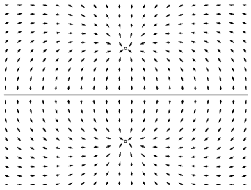
Figure 7.6.1: In black the vector field on the chart $U$. The horizontal line on the center is part of a whole $S^{1}$ of zeroes of $\xi_{0}$

Following the proof of Lemma 7.2.1, modulo the unit $(1+|v|^{2})$ that only scales the vector field, we can compute

$$\lim_{u\to 0}|u|^{2}\left(\begin{matrix}-\frac{2}{\bar{u}\bar{v}^{2}+\bar{u}}\\ \frac{2{\left(v-\bar{v}\right)}}{u\bar{u}\bar{v}^{2}+u\bar{u}}\end{matrix}\right)=\left(\begin{matrix}0\\ \frac{2{\left(v-\bar{v}\right)}}{\bar{v}^{2}+1}\end{matrix}\right).$$

That is, for the chart $U\cap D_{0}^{\circ}$ with coordinate $v$,

$$\xi_{0}=\frac{2{\left(v-\bar{v}\right)}}{\bar{v}^{2}+1}.$$

We can see from the expression above that the vector field has non-isolated zeroes (see Fig. 7.6.1). More concretely, the whole line $\mathop{\mathrm{Re}}(v)=0$ is a line of zeros in $U\cap D_{0}^{\circ}$. Actually, this line forms part of a $S^{1}$ of zeroes in $D_{0}^{\circ}$. In particular, this shows that the standard metric here does not come from a matrix $A$ in $G_{0}$ (Definition 7.4.10) since the vector field cannot be Morse for any function.

In the next example we consider the Morse singularity obtained from $y^{2}+x^{2}$ after the linear change of coordinates $y\mapsto y$ and $x\mapsto x+y$.

Example 7.6.2.

Consider the polynomial $f(x,y)=y^{2}+(y+x)^{2}$. Let $\pi_{0}:Y_{0}\to{\mathrm{Tub}}$ and $U\subset Y_{0}$ as before. We find:

$$\pi_{0}^{*}f=\left(2v^{2}+2v+1\right)u^{2},\quad\mathop{\mathrm{Jac}}\pi_{0}=\begin{pmatrix}1&0\\ v&u\end{pmatrix},\quad\det\mathop{\mathrm{Jac}}\pi_{0}=u.$$

And so, following eq. 7.1.2, we find

$$\left(\begin{matrix}\xi^{u}\\ \xi^{v}\end{matrix}\right)=\frac{-1}{u\left(2\bar{v}^{2}+2\bar{v}+1\right)\bar{u}^{2}}\left(\begin{matrix}2\bar{u}\bar{v}+2\bar{u}\\ 4\bar{u}\bar{v}+2\bar{u}\end{matrix}\right)=\left(\begin{matrix}-\frac{2{\left(\bar{v}+1\right)}}{2\bar{u}\bar{v}^{2}+2\bar{u}\bar{v}+\bar{u}}\\ \frac{2{\left({\left(v-2\right)}\bar{v}+v-1\right)}}{2u\bar{u}\bar{v}^{2}+2u\bar{u}\bar{v}+u\bar{u}}\end{matrix}\right).$$

As before, we now compute the scaling and extension of

$$\lim_{u\to 0}|u|^{2}\left(\begin{matrix}-\frac{2{\left(\bar{v}+1\right)}}{2\bar{u}\bar{v}^{2}+2\bar{u}\bar{v}+\bar{u}}\\ \frac{2{\left({\left(v-2\right)}\bar{v}+v-1\right)}}{2u\bar{u}\bar{v}^{2}+2u\bar{u}\bar{v}+u\bar{u}}\end{matrix}\right)=\left(\begin{matrix}0\\ \frac{2{\left({\left(v-2\right)}\bar{v}+v-1\right)}}{2\bar{v}^{2}+2\bar{v}+1}\end{matrix}\right).$$

So on $U\cap D_{0}^{\circ}$ we have the expression,

$$\xi_{0}=\frac{2{\left({\left(v-2\right)}\bar{v}+v-1\right)}}{2\bar{v}^{2}+2\bar{v}+1}.$$

This vector field has isolated singularities on $D_{0}^{\circ}$ at the points

$$p_{0}=(1-\sqrt{5})/2,\quad p_{1}=(1+\sqrt{5})/2.$$

We compute the Hessian of $\xi_{0}$ at those singularities. For that we write $v=s+it$ and compute the partials of the vector field evaluated at those points. For $p_{0}$ we get:

$$\begin{split}\left.\partial_{s}\xi_{0}\right|_{((1-\sqrt{5})/2,0)}&=-\frac{4{\left({\left(s+it-2\right)}{\left(s-it\right)}+s+it-1\right)}{\left(2s-2it+1\right)}}{{\left(2{\left(s-it\right)}^{2}+2s-2it+1\right)}^{2}}\\ &\left.+\frac{2{\left(2s-1\right)}}{2{\left(s-it\right)}^{2}+2s-2it+1}\right|_{((1-\sqrt{5})/2,0)}\\ &=\frac{-2\sqrt{5}}{5-2\sqrt{5}}\end{split}$$

and

$$\begin{split}\left.\partial_{t}\xi_{0}\right|_{(1-\sqrt{5})/2,0)}&=-\frac{4{\left({\left(s+it-2\right)}{\left(s-it\right)}+s+it-1\right)}{\left(-2is-2t-i\right)}}{{\left(2{\left(s-it\right)}^{2}+2s-2it+1\right)}^{2}}\\ &\left.+\frac{2{\left(2t+3i\right)}}{2{\left(s-it\right)}^{2}+2s-2it+1}\right|_{(1-\sqrt{5})/2,0)}\\ &=\frac{6i}{5-2\sqrt{5}}\end{split}$$

So the Hessian is, up to a positive real constant,

$${\mathrm{Hess}}_{((1-\sqrt{5})/2,0)}\xi_{0}=\begin{pmatrix}\frac{-2\sqrt{5}}{5-2\sqrt{5}}&0\\ 0&\frac{6}{5-2\sqrt{5}}\end{pmatrix},$$

which indicates that $p_{0}$ is a saddle point. A similar computation for $p_{1}$ leads to the Hessian

$${\mathrm{Hess}}_{((1+\sqrt{5})/2,0)}\xi_{0}=\begin{pmatrix}\frac{2\sqrt{5}}{2\sqrt{5}+5}&0\\ 0&\frac{6}{2\sqrt{5}+5}\end{pmatrix}.$$

That is, $p_{1}$ is a fountain (see Fig. 7.6.2).

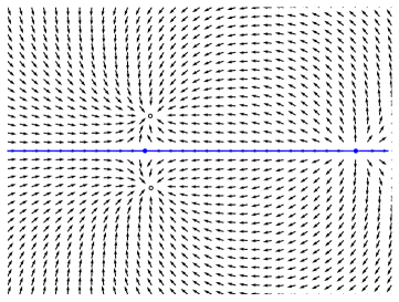
Figure 7.6.2: In black the vector field on the chart $U$. In this case the vector field has a potential which is a Morse function so all the zeroes are isolated. We see a saddle point and a fountain. In blue the spine $S_{0}$

Figure 7.6.3: On the left we see the exceptional set of $Y_{0}$, the vector field in black and the spine $S_{0}$ in blue. On the right we see the corresponding picture for a fixed angled on the Milnor fiber at radius zero.

Figure 7.6.4: The inner cylinder represents the Milnor fiber at radius $0$ and angle $t$. The outer cylinder represents a Milnor fiber over a point $t$ with $\arg(t)=\theta$. In light blue we see the closure of the union of all trajectories starting at the Milnor fiber $F_{t}$ that converge to some point in the Milnor fiber at radius $0$. In darker blue we see some of the trajectories together with the spine $S_{t}$ on the Milnor fiber $F_{t}$ and the spine $S^{\mathrm{ro}}_{0,\theta}$ at radius $0$ and angle $\theta$.

Example 7.6.3.

Let $f(x,y)=y^{3}+x^{3}$ and let $\pi_{0}:Y_{0}\to{\mathrm{Tub}}$ be the blow up at the origin $0\in{\mathrm{Tub}}$. Take the local chart $U\subset Y_{0}$ with coordinates $u,v$ such that

$$\pi_{0}(u,v)=(u,uv).$$

In these local coordinates we have:

$$\pi_{0}^{*}f=u^{3}{\left(v^{2}-v+1\right)}{\left(v+1\right)},\quad\mathop{\mathrm{Jac}}\pi_{0}=\begin{pmatrix}1&0\\ v&u\end{pmatrix},\quad\det\mathop{\mathrm{Jac}}\pi_{0}=u.$$

And so, following eq. 7.1.2, we find

$$\left(\begin{matrix}\xi^{u}\\ \xi^{v}\end{matrix}\right)=\frac{1}{u{\left(\bar{v}^{2}-\bar{v}+1\right)}{\left(\bar{v}+1\right)}\bar{u}^{3}}\left(\begin{matrix}3u\bar{u}^{2}\\ -3v\bar{u}^{2}+3\bar{u}^{2}\bar{v}^{2}\end{matrix}\right)=\left(\begin{matrix}-\frac{3}{\bar{u}\bar{v}^{3}+\bar{u}}\\ -\frac{3{\left(\bar{v}^{2}-v\right)}}{u\bar{u}\bar{v}^{3}+u\bar{u}}\end{matrix}\right).$$

Following the proof of Lemma 7.2.1, modulo the unit $(1+|v|^{2})$ that only scales the vector field, we can compute

$$\lim_{u\to 0}|u|^{2}\left(\begin{matrix}-\frac{3}{\bar{u}\bar{v}^{3}+\bar{u}}\\ -\frac{3{\left(\bar{v}^{2}-v\right)}}{u\bar{u}\bar{v}^{3}+u\bar{u}}\end{matrix}\right)=\left(\begin{matrix}0\\ -\frac{3{\left(\bar{v}^{2}-v\right)}}{\bar{v}^{3}+1}\end{matrix}\right).$$

That is, for the chart $U\cap D_{0}^{\circ}$ with coordinate $v$,

$$\xi_{0}=-\frac{3{\left(\bar{v}^{2}-v\right)}}{\bar{v}^{3}+1}.$$

A direct computation, shows that this vector field vanishes at the origin and at the $3$rd roots of unity, that is, at the points

$$v=0,\quad v=1,\quad v=-1/2(1+i\sqrt{3}),\quad v=1/2(-1+i\sqrt{3}).$$

Next we compute the Hessian of $\xi_{0}$ at those points. Take real coordinates $s,t$ such that $v=s+it$. We compute the partials and evaluate at $(s,t)=(0,0)$

$$\left.\partial_{s}\xi_{0}\right|_{(0,0)}=\left.\frac{9{\left({\left(s-it\right)}^{2}-s-it\right)}{\left(s-it\right)}^{2}}{{\left({\left(s-it\right)}^{3}+1\right)}^{2}}-\frac{3{\left(2s-2it-1\right)}}{{\left(s-it\right)}^{3}+1}\right|_{(0,0)}=3$$

and

$$\left.\partial_{t}\xi_{0}\right|_{(0,0)}=\left.-\frac{9i{\left({\left(s-it\right)}^{2}-s-it\right)}{\left(s-it\right)}^{2}}{{\left({\left(s-it\right)}^{3}+1\right)}^{2}}-\frac{3{\left(-2is-2t-i\right)}}{{\left(s-it\right)}^{3}+1}\right|_{(0,0)}=3i$$

which yields the Hessian

$${\mathrm{Hess}}_{(0,0)}\xi_{0}=\begin{pmatrix}3&0\\ 0&3\end{pmatrix},$$

that shows that $\xi_{0}$ has a fountain at the origin.

When $v=1$, that is $(s,t)=(1,0)$, we have

$${\mathrm{Hess}}_{(1,0)}\xi_{0}=\begin{pmatrix}-3/2&0\\ 0&9/2\end{pmatrix},$$

which shows that $\xi_{0}$ has a saddle point at $(1,0)$. A similar computation shows that $\xi_{0}$ has also saddle points at $(-1/2,-\sqrt{3}/2)$ and $(-1/2,\sqrt{3}/2)$. So, in the chart $U$, the vector field looks as in Fig. 7.6.5.

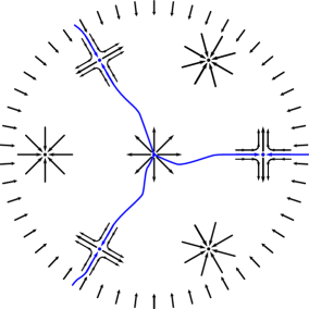
Figure 7.6.5: In black the vector field on the chart $U$. The inwards pointing outer arrows indicate that there is a fountain at infinity (or rather at the only point of $D_{0}$ that $U$ does not see). In blue the stable manifolds of the three saddle points.

By taking another chart, an analogous computations yields that $\xi_{0}$ has a fountain at the only point in $D_{0}^{\circ}$ not seen by the chart $U$.

The Milnor fiber at radius $0$ minus a tubular neighborhood of its boundary is a $3$-fold regular cover of $D_{0}^{\circ}$. Therefore, each of the two fountains give rise to $3$ vertices of the spine at radius $0$.

8 The vector field near the corners

Near an intersection point $D_{i}\cap D_{j}$ of two exceptional components in $Y$, the pull-back of $\xi$ has poles along $D_{i}\cap D_{j}$. Assuming that the edge $ij$ is invariant, Definition 6.1.1 after rescaling $\pi^{*}(\xi)$ by a positive factor, the vector field extends to an analytic vector field near $D_{i}\cap D_{j}$, which does not vanish identically along $D_{i}$ or $D_{j}$. If the edge is not invariant, a similar scaling of the further pullback $(\pi^{\mathrm{ro}})^{*}(\xi)$ to the real oriented blow-up extends over the boundary. The vanishing order of this positive factor is given by the radial weights $\tau_{i}$ defined below.

In this section we work with the resolution $\pi_{\mathrm{pol}}:Y_{\mathrm{pol}}\to\mathbb{C}^{2}$ which, in particular, resolves generic polar curves (see Definition 5.1.2). We use the notation $\pi=\pi_{\mathrm{pol}}$.

Definition 8.0.1.

The radial weight of the vertex $i\in\mathcal{V}$ is the integer

$$\tau_{i}=c_{1,i}+m_{i}-p_{i}.$$

Remark 8.0.2.

It follows from definition that $\tau_{i}+\varpi_{i}=2c_{1,i}$. By Lemma 6.1.3, we therefore have $\tau_{i}\leq 2c_{1,i}$ for all $i\in\mathcal{V}$. Equality holds precisely for the invariant vertices, i.e. when $i\in\mathcal{V}_{\Upsilon}$, by Lemma 6.2.3. In particular, $\tau_{i}$ is even in this case.

8.0.3.

Let $i,j\in\mathcal{V}$, and assume that there is a directed edge $j\to i$ in $\Gamma$ (see Definition 3.4.1). Note that this implies that $i\neq 0$, since all edges adjacent to $0$ point away from $0$. Corresponding to the edge $ij$, we have an intersection point $p\in D_{i}\cap D_{j}$. Choose isometric coordinates $x,y$ in $\mathbb{C}^{2}$ so that $y=0$ defines the tangent associated with $p$ (see Definition 3.5.1). Let $U\subset Y$ be a small chart containing $p$ with coordinates $u,v$. We choose $u,v$ in such a way that

(8.0.4) $$\begin{split}\pi^{*}x&=u^{c_{0,i}}v^{c_{0,j}}\\ \pi^{*}y&=u^{k}v^{\ell}\eta(u,v)\end{split}$$

where $\eta(0,0)\neq 0$. Since $i\neq 0$, we have $k>c_{0,i}$ (Lemma 3.5.2). Similarly, $\ell\geq c_{0,j}$ with equality if and only if $j=0$.

On $U\setminus D$, we have an explicit description of the pullback of $\xi$

(8.0.5) $$\pi|_{U\setminus D}^{*}\xi=\begin{pmatrix}\xi^{u}\\ \xi^{v}\end{pmatrix}=\frac{-1}{\det\mathop{\mathrm{Jac}}\pi\cdot\bar{f}}\begin{pmatrix}y_{v}\bar{f}_{x}-x_{v}\bar{f}_{y}\\ -y_{u}\bar{f}_{x}+x_{u}\bar{f}_{y}\end{pmatrix}$$

Since $f_{y}$ defines a generic polar curve (by the definition of $\pi_{\mathrm{pol}}$ and the assumption on the coordinate $y$), it vanishes along $D_{i},D_{j}$ with multiplicities $p_{i},p_{j}$, we can write $\pi^{*}f_{y}(u,v)=u^{p_{i}}v^{p_{j}}(b+{\mathrm{h.o.t.}})$ where $b\in\mathbb{C}^{*}$. We can therefore explicitly write

$$x_{v}\bar{f}_{y}=u^{c_{0,i}}\bar{u}^{p_{i}}v^{c_{0,j}-1}\bar{v}^{p_{j}}(c_{0,j}\bar{b}+{\mathrm{h.o.t.}})$$

with $b\in\mathbb{C}^{*}$. Here, once again, we are identifying $f_{y}$ with its pullback. We can now write $\pi^{*}f_{x}(u,v)=u^{p_{i}^{\prime}}v^{p_{j}^{\prime}}(b^{\prime}+{\mathrm{h.o.t.}})$ with the inequalities $p_{i}^{\prime}\geq p_{i}$ and $p_{j}^{\prime}\geq p_{j}$ because the $x$-axis is a tangent by hypothesis. Again using the observation after eq. 8.0.4, we can write

$$y_{v}\bar{f}_{x}=u^{k}\bar{u}^{p_{i}^{\prime}}v^{\ell-1}\bar{v}^{p_{j}^{\prime}}(\ell b^{\prime}+{\mathrm{h.o.t.}})=u^{c_{0,i}}\bar{u}^{p_{i}}v^{c_{0,j}-1}\bar{v}^{p_{j}}(0+{\mathrm{h.o.t.}})$$

with $b^{\prime}\in\mathbb{C}$. Together this yields

$$y_{v}\bar{f}_{x}-x_{v}\bar{f}_{y}=u^{c_{0,i}}\bar{u}^{p_{i}}v^{c_{0,j}-1}\bar{v}^{p_{j}}(-c_{0,j}\bar{b}+{\mathrm{h.o.t.}}).$$

By an analogous reasoning we find,

$$-y_{u}\bar{f}_{x}+x_{u}\bar{f}_{y}=u^{c_{0,i}-1}\bar{u}^{p_{i}}v^{c_{0,j}}\bar{v}^{p_{j}}(c_{0,i}\bar{b}+{\mathrm{h.o.t.}}).$$

Similarly, we can also write

(8.0.6) $$\begin{split}\pi^{*}f(u,v)&=u^{m_{i}}v^{m_{j}}(a+{\mathrm{h.o.t.}})\quad a\in\mathbb{C}^{*}\\ \det\mathop{\mathrm{Jac}}\pi(u,v)&=u^{\nu_{i}-1}v^{\nu_{j}-1}(c+{\mathrm{h.o.t.}})\quad c\in\mathbb{C}^{*}.\end{split}$$

Setting $d=\bar{b}/(c\bar{a})\in\mathbb{C}^{*}$, we get

(8.0.7) $$|u|^{\tau_{i}}|v|^{\tau_{j}}\pi|_{U\setminus D}^{*}\xi=\left(\frac{u}{|u|}\right)^{\varpi_{i}}\left(\frac{v}{|v|}\right)^{\varpi_{j}}d\left(\begin{matrix}u(c_{0,j}+{\mathrm{h.o.t.}})\\ v(-c_{0,i}+{\mathrm{h.o.t.}})\end{matrix}\right).$$

The previous discussion, in particular the above equation, yields the following result.

Lemma 8.0.8.

• If $p\in D_{i}\cap D_{j}$ is an invariant intersection point, then the vector field

  (8.0.9) $$|u|^{\tau_{i}}|v|^{\tau_{j}}\pi|_{U\setminus D}^{*}\xi$$

  extends to an analytic vector field on $U$ that is tangent to $D_{i}\cap U$ and $D_{j}\cap U$. And it does not vanish identically there.

• The scaled pull-back

  (8.0.10) $$r^{\tau_{i}}s^{\tau_{j}}\pi^{\mathrm{ro}}|_{U^{\mathrm{ro}}\setminus\partial U^{\mathrm{ro}}}^{*}\xi$$

  extends to an analytic vector field on $U^{\mathrm{ro}}$, which is tangent to both $D^{\mathrm{ro}}_{i}\cap U^{\mathrm{ro}}$ and $D^{\mathrm{ro}}_{j}\cap U^{\mathrm{ro}}$. Furthermore, if $ij$ is a non-invariant edge, it does not vanish identically along $D^{\mathrm{ro}}_{i,j}$. ∎

Definition 8.0.11.

Denote by $\xi^{\mathrm{ro}}_{U}$ the analytic vector field on $U^{\mathrm{ro}}$ whose restriction to $U^{\mathrm{ro}}\setminus\partial U^{\mathrm{ro}}$ coincides with eq. 8.0.10. We denote by $\xi^{\mathrm{ro}}_{i,j,\theta}$ the restriction of $\xi^{\mathrm{ro}}_{U}$ to a neighborhood of $D^{\mathrm{ro}}_{i,j,\theta}$ in the Milnor fiber $F^{\mathrm{ro}}_{\theta}$ at radius $0$ and angle $\theta$.

Similarly, for $p$ an invariant intersection point, denote by $\xi_{U}$ the analytic vector field on $U$ whose restriction to $U\setminus D$ coincides with eq. 8.0.9.

8.1 Invariant intersection points

In this subsection we consider an invariant edge $ij$ in the graph $\Gamma$. We use the notation from 8.0.3, and assume $\varpi_{i}=\varpi_{j}=0$ and that $j\to i$.

Lemma 8.1.1.

If $p\in D_{i}\cap D_{j}$ is an invariant intersection point, then the vector field $\xi_{U}$ has an elementary singularity at $p$, whose unstable manifold is $D_{i}$ and whose stable manifold is $D_{j}$.

Proof.

The statement on the stable and unstable manifold follows as soon as we show that $d$ from eq. 8.0.7 is a positive real number:

Denote by $l$ the coefficient of $u^{c_{1,i}}v^{c_{1,j}}$ in the expansion of $\pi^{*}y$ in $u,v$. We have

$$\det\mathop{\mathrm{Jac}}\pi(u,v)=x_{u}y_{v}-x_{v}y_{v}=c_{0,i}u^{c_{0,i}-1}v^{c_{0,j}}y_{v}-c_{0,j}u^{c_{0,i}}v^{c_{0,j}-1}y_{u},$$

and so we can compute the number $c$ from eq. 8.0.6:

$$c=(c_{0,i}c_{1,j}-c_{0,j}c_{1,i})l.$$

A chain rule computation gives

$$\begin{split}f_{y}&=\frac{-x_{v}f_{u}+x_{u}f_{v}}{x_{u}y_{v}-y_{u}x_{v}}\\ &=\frac{u^{c_{0,i}+m_{i}-1}v^{c_{0,j}+m_{j}-1}(a(c_{0,j}m_{i}-c_{0,i}m_{j})+{\mathrm{h.o.t.}})}{u^{\nu_{i}-1}v^{\nu_{j}-1}(c+{\mathrm{h.o.t.}})}\\ &=-\frac{a}{c}\cdot\left|\begin{matrix}c_{0,i}&m_{i}\\ c_{0,j}&m_{j}\end{matrix}\right|(u^{p_{i}}v^{p_{j}}+{\mathrm{h.o.t.}})\end{split}$$

and so $b=a(m_{i}c_{0,j}-m_{j}c_{0,i})/c$, i.e. $d=\bar{b}/(c\bar{a})=(m_{i}c_{0,j}-m_{j}c_{0,i})/|c|^{2}>0$ where the last inequality follows from the fact that $(c_{0,i}m_{j}-m_{i}c_{0,j})<0$ by Lemma 3.4.5. Since $d$ is positive, the result follows from Grobman-Hartman theorem and eq. 8.0.7. ∎

The previous lemma talks about the Hessian of the vector field $\xi_{U}$ in $Y_{\mathrm{pol}}$, it is also useful later on the text to be able to speak about the Hessian of the vector field $\xi^{\mathrm{ro}}_{U}$ in $Y^{\mathrm{ro}}_{\mathrm{pol}}$.

8.1.2.

Here we briefly explain how to obtain useful formulas for the pullback of our vector field to $Y^{\mathrm{ro}}$. We use polar coordinates $r$, $s$, $\alpha$ and $\beta$ (in this order), where $u=re^{i\alpha}$, $v=se^{i\beta}$ for the chart $U^{\mathrm{ro}}=\sigma^{-1}(U)\subset Y^{\mathrm{ro}}$. We can write

$$\xi^{\mathrm{ro}}_{U}=(\xi^{\mathrm{ro},r},\xi^{\mathrm{ro},s},\xi^{\mathrm{ro},\alpha},\xi^{\mathrm{ro},\beta})^{\top}.$$

The formulas

(8.1.3) $$\xi^{\mathrm{ro},r} =\mathop{\mathrm{Re}}(e^{-i\alpha}\sigma^{*}\xi^{u}),\qquad \xi^{\mathrm{ro},s} =\mathop{\mathrm{Re}}(e^{-i\beta}\sigma^{*}\xi^{v}),$$

$$\xi^{\mathrm{ro},\alpha} =\mathop{\mathrm{Im}}(r^{-1}e^{-i\alpha}\sigma^{*}\xi^{u}),\qquad \xi^{\mathrm{ro},\beta} =\mathop{\mathrm{Im}}(s^{-1}e^{-i\beta}\sigma^{*}\xi^{v}),$$

follow from a direct computation in polar coordinates. Next, we carry on this direct computation of the formulas for $\xi^{\mathrm{ro},r}$. We observe that in $U^{\mathrm{ro}}$, the real oriented blow up $\sigma$ is expressed as

$$(r,s,\alpha,\beta)\mapsto(re^{i\alpha},se^{i\beta})$$

and so its Jacobian is

$$\mathop{\mathrm{Jac}}\sigma=\left(\begin{matrix}\cos\alpha&0&-r\sin\alpha&0\\ \sin\alpha&0&r\cos\alpha&0\\ 0&\cos\beta&0&-s\sin\beta\\ 0&\sin\beta&0&s\cos\beta\end{matrix}\right).$$

This matrix is, up to permutation of the second and third columns, a block diagonal matrix. So we can compute its inverse by blocks and find that

(8.1.4) $$(\mathop{\mathrm{Jac}}\sigma)^{-1}=\left(\begin{matrix}\cos\alpha&0&\sin\alpha&0\\ -\frac{\sin\alpha}{r}&0&\frac{\cos\alpha}{r}&0\\ 0&\cos\beta&0&\sin\beta\\ 0&-\frac{\sin\beta}{s}&0&s\frac{\cos\beta}{s}\end{matrix}\right).$$

By definition of the pullback of a vector field we know that

$$\xi^{\mathrm{ro}}_{U}=(\mathop{\mathrm{Jac}}\sigma)^{-1}(\mathop{\mathrm{Re}}(\sigma^{*}\xi^{u}),\mathop{\mathrm{Im}}(\sigma^{*}\xi^{u}),\mathop{\mathrm{Re}}(\sigma^{*}\xi^{v}),\mathop{\mathrm{Im}}(\sigma^{*}\xi^{v}))^{\top}.$$

So using eq. 8.1.4, we compute, on one hand:

(8.1.5) $$\xi^{\mathrm{ro},r}=(\cos\alpha)\cdot\mathop{\mathrm{Re}}(\sigma^{*}\xi^{u})+(\sin\alpha)\cdot\mathop{\mathrm{Im}}(\sigma^{*}\xi^{u}).$$

And on the other hand:

(8.1.6) $$\begin{split}\mathop{\mathrm{Re}}(e^{-i\alpha}\sigma^{*}(\xi^{u}))=&\mathop{\mathrm{Re}}\left((\cos\alpha-i\sin\alpha)\cdot(\mathop{\mathrm{Re}}(\sigma^{*}\xi^{u})+i\mathop{\mathrm{Im}}(\sigma^{*}\xi^{u}))\right)\\ =&\mathop{\mathrm{Re}}\left((\cos\alpha)\cdot\mathop{\mathrm{Re}}(\sigma^{*}\xi^{u})+(\sin\alpha)\cdot\mathop{\mathrm{Im}}(\sigma^{*}\xi^{u})\right.\\ &\left.+i\left((\cos\alpha)\cdot\mathop{\mathrm{Im}}(\sigma^{*}\xi^{u})-(\sin\alpha)\cdot\mathop{\mathrm{Re}}(\sigma^{*}\xi^{u})\right)\right)\\ =&(\cos\alpha)\cdot\mathop{\mathrm{Re}}(\sigma^{*}\xi^{u})+(\sin\alpha)\cdot\mathop{\mathrm{Im}}(\sigma^{*}\xi^{u})\end{split}$$

From eq. 8.1.5 and eq. 8.1.6, we verify the formula for $\xi^{\mathrm{ro},r}$ given in eq. 8.1.3. The other three formulas of eq. 8.1.3 follow from very similar computations.

Corollary 8.1.7.

At a point $q\in D^{\mathrm{ro}}_{i,j}$ with $\varpi_{i}=\varpi_{j}=0$, the vector field $\xi^{\mathrm{ro}}_{U}$ has a Hessian

$${\mathrm{Hess}}_{q}\xi^{\mathrm{ro}}_{U}=\left(\begin{matrix}dc_{0,j}&0&0&0\\ 0&-dc_{0,i}&0&0\\ 0&0&0&0\\ 0&0&0&0\end{matrix}\right).$$

Moreover, there exists a local change of coordinates such that

$$\xi^{\mathrm{ro}}_{i,j,\theta}=(dc_{0,j}r^{\prime},-dc_{0,i}s^{\prime},0,0)^{\top}.$$

in coordinates $r^{\prime},s^{\prime},\alpha^{\prime},\beta^{\prime}.$

Proof.

Using eq. 8.1.3 and eq. 8.0.7 we get

$$\xi^{\mathrm{ro},r}=\mathop{\mathrm{Re}}(e^{-i\alpha}dre^{i\alpha}(c_{0,j}+{\mathrm{h.o.t.}}))=rdc_{0,j}+\mathop{\mathrm{Re}}({\mathrm{h.o.t.}})$$

where $\mathop{\mathrm{Re}}({\mathrm{h.o.t.}})$ denotes the real part of the higher (than linear) order terms. This yields the first row of the Hessian in the statement. Similarly, we find

$$\xi^{\mathrm{ro},\alpha}=\mathop{\mathrm{Im}}(r^{-1}e^{-i\alpha}dre^{i\alpha}(c_{0,j}+{\mathrm{h.o.t.}})))=\mathop{\mathrm{Im}}(dc_{0,j}+{\mathrm{h.o.t.}})=0+\mathop{\mathrm{Im}}({\mathrm{h.o.t.}}),$$

which gives the third row of the Hessian. The second and fourth rows are completely analogous.

For the last statement we use that the vector field $\xi_{U}$ satisfies the hypothesis of the Grobman-Hartman theorem by Lemma 8.1.1. This implies that there exists coordinates $u^{\prime},v^{\prime}$ for $U$ such that $\{u^{\prime}=0\}=D_{i}\cap U$ and $\{v^{\prime}=0\}=D_{j}\cap U$ and such that $\xi_{U}$ in the coordinates $u^{\prime},v^{\prime}$ is

(8.1.8) $$\left(\begin{matrix}\xi^{u^{\prime}}\\ \xi^{v^{\prime}}\end{matrix}\right)=\left(\begin{matrix}dc_{0,j}u^{\prime}\\ -dc_{0,i}v^{\prime}\end{matrix}\right).$$

So, after taking its pullback by the real oriented blow up $\sigma(r^{\prime},\alpha^{\prime},s^{\prime},\beta^{\prime})=(r^{\prime}e^{i\alpha^{\prime}},s^{\prime}e^{i\beta^{\prime}})$, we get the vector field

(8.1.9) $$\xi^{\mathrm{ro}}_{U}=(dc_{0,j}r^{\prime},-dc_{0,i}s^{\prime},0,0)^{\top}$$

which proves the last statement. ∎

In fig. 8.1.1 we can see a drawing of the vector field $\xi^{\mathrm{ro}}_{U}$ restricted to $(D^{\mathrm{ro}}_{i,\theta}\cup D^{\mathrm{ro}}_{j,\theta})\cap U$

Figure 8.1.1: The vector field $\xi^{\mathrm{ro}}_{U}$ restricted to $(D^{\mathrm{ro}}_{i,\theta}\cup D^{\mathrm{ro}}_{j,\theta})\cap U$ near a component of $D^{\mathrm{ro}}_{i,j,\theta}$ for an edge $j\to i$ and with $\varpi_{i}=\varpi_{j}=0$.

8.2 Noninvariant intersection points

Next we assume that $\varpi_{i},\varpi_{j}$ are not both 0. In this subsection we also use the formulas eq. 8.1.3.

Lemma 8.2.1.

In polar coordinates given by the real oriented blow up, the following expression holds

$$\arg(f)(0,0,\alpha,\beta)=m_{i}\alpha+m_{j}\beta+\Delta$$

with $\Delta\in\mathbb{R}/2\pi\mathbb{Z}$ a constant.

Proof.

This follows from Lemma 4.1.2 and the observation that $\arg(f)(0,0,\alpha,\beta)$ is equivariant with respect to $\cdot_{i}$ of weight $m_{i}$ and equivariant with respect to $\cdot_{j}$ of weight $m_{j}$. ∎

Definition 8.2.2.

With $d\in\mathbb{C}^{*}$ as in 8.0.3, set $\delta=\arg(d)\in\mathbb{R}/2\pi\mathbb{Z}$, and

(8.2.3) $$\begin{split}\Sigma_{i,j}^{+}&=\left\{(0,0,\alpha,\beta)\in U^{\mathrm{ro}}\,\middle|\,\delta+\varpi_{i}\alpha+\varpi_{j}\beta\equiv 0\;(\mathop{\rm mod}\nolimits 2\pi\mathbb{Z})\right\}\subset D^{\mathrm{ro}}_{i,j},\\ \Sigma_{i,j}^{-}&=\left\{(0,0,\alpha,\beta)\in U^{\mathrm{ro}}\,\middle|\,\delta+\varpi_{i}\alpha+\varpi_{j}\beta\equiv\pi\;(\mathop{\rm mod}\nolimits 2\pi\mathbb{Z})\right\}\subset D^{\mathrm{ro}}_{i,j},\end{split}$$

and $\Sigma_{i,j}=\Sigma_{i,j}^{+}\cup\Sigma_{i,j}^{-}$.

Lemma 8.2.4.

Fix $\theta\in\mathbb{R}/2\pi\mathbb{Z}$.

• The set $\Sigma_{i,j}$ is a real $1$-dimensional affine subspace homeomorphic to a disjoint union of $2\gcd(\varpi_{i},\varpi_{j})$ circles.

• The set $D^{\mathrm{ro}}_{i,j}\cap Y^{\mathrm{ro}}_{\theta}$ is a real $1$-dimensional affine subspace homeomorphic to a disjoint union of $\gcd(m_{i},m_{j})$ circles.

• The intersection $\Sigma_{i,j}\cap Y^{\mathrm{ro}}_{\theta}$ is transverse and

  $$|\Sigma^{+}_{i,j}\cap Y^{\mathrm{ro}}_{\theta}|=|\Sigma^{-}_{i,j}\cap Y^{\mathrm{ro}}_{\theta}|=-\left|\begin{matrix}m_{i}&\varpi_{i}\\ m_{j}&\varpi_{j}\end{matrix}\right|.$$

Proof.

The map $\chi:D^{\mathrm{ro}}_{i,j}\to\mathbb{R}/2\pi\mathbb{Z}$, $(\alpha,\beta)\mapsto\delta+\varpi_{i}\alpha+\varpi_{j}\beta$ with $\delta=\arg(d)$, is a surjective affine morphism, and therefore its preimages $\chi^{-1}(0)$ and $\chi^{-1}(\pi)$ are submanifolds of dimension $\dim_{\mathbb{R}}D^{\mathrm{ro}}_{i,j}-\dim_{\mathbb{R}}(\mathbb{R}/2\pi\mathbb{Z})=1$. From eq. 8.2.3 we see that $\Sigma^{\pm}_{i,j}$ consists of $\gcd(\varpi_{i},\varpi_{j})$ connected components. In fact, each component can be parametrized as follows. Set $(\varpi_{i}^{\prime},\varpi_{j}^{\prime})=(\varpi_{i},\varpi_{j})/\gcd(\varpi_{i},\varpi_{j})$. We see that $\Sigma_{i,j}$ consists of components parametrized by $\gamma\in\mathbb{R}/2\pi\mathbb{Z}$ by

$$r=s=0,\quad\alpha=-\varpi^{\prime}_{j}\gamma+\delta^{\prime},\quad\beta=\varpi^{\prime}_{i}\gamma+\delta^{\prime\prime}$$

where $\delta^{\prime}$ and $\delta^{\prime\prime}$ are some constants in $\mathbb{R}/2\pi\mathbb{Z}$.

A similar argument works for the set $D^{\mathrm{ro}}_{i,j}\cap Y^{\mathrm{ro}}_{\theta}$ since

(8.2.5) $$D^{\mathrm{ro}}_{i,j}\cap Y^{\mathrm{ro}}_{\theta}=\left\{(0,0,\alpha,\beta)\in U^{\mathrm{ro}}\,\middle|\,m_{i}\alpha+m_{j}\beta+\Delta=\theta\right\}.$$

The composition

$$\arg(f)(0,0,-\varpi^{\prime}_{j}\gamma,\varpi^{\prime}_{i}\gamma)=\frac{m_{j}\varpi_{i}-m_{i}\varpi_{j}}{\gcd(\varpi_{i},\varpi_{j})}\cdot\gamma+\Delta$$

is a submersion, since $m_{i}\varpi_{j}-m_{j}\varpi_{i}<0$ by 6.3.7 and 6.3.6 item (v). which proves transversality. ∎

Lemma 8.2.6.

Let $\theta\in\mathbb{R}/2\pi\mathbb{Z}$, let $i,j\in\mathcal{V}_{\mathrm{pol}}$ and assume that the edge $ij$ exists and $j\to i$.

• The vanishing set of $\xi^{\mathrm{ro}}_{U}$ is $\Sigma_{i,j}$.

• The Hessian of $\xi^{\mathrm{ro}}_{U}$ along the normal bundle of $\Sigma_{i,j}$ is elementary.

• If $q\in\Sigma_{i,j}^{+}$ and $\arg(f)(q)=\theta$, then the unstable manifold of $\xi^{\mathrm{ro}}_{U}$ at $q$ is the germ $(D^{\mathrm{ro}}_{i,\theta},q)$, and its stable manifold is a single trajectory in $(D^{\mathrm{ro}}_{j,\theta},q)$.

• Similarly, if $q\in\Sigma_{i,j}^{-}$ and $\arg(f)(q)=\theta$, then the stable manifold of $\xi^{\mathrm{ro}}_{U}$ at $q$ is $(D^{\mathrm{ro}}_{i,\theta},q)$, and its unstable manifold is a single trajectory in $(D^{\mathrm{ro}}_{j,\theta},q)$.

Lemma 8.2.7.

Let $q\in\Sigma_{i,j}$. Set $\chi(\alpha,\beta)=\delta+\varpi_{i}\alpha+\varpi_{j}\beta$ with $\delta=\arg(d)$. Then

(8.2.8) $$\begin{split}r^{\tau_{i}}s^{\tau_{j}}\xi^{\mathrm{ro},r}&\in r|d|c_{0,j}\cos(\chi(\alpha,\beta))+\mathfrak{m}^{2}_{Y^{\mathrm{ro}},q}\\ r^{\tau_{i}}s^{\tau_{j}}\xi^{\mathrm{ro},s}&\in-s|d|c_{0,i}\cos(\chi(\alpha,\beta))+\mathfrak{m}^{2}_{Y^{\mathrm{ro}},q},\\ r^{\tau_{i}}s^{\tau_{j}}\xi^{\mathrm{ro},\alpha}&\in|d|c_{0,j}\sin(\chi(\alpha,\beta))+\mathfrak{m}^{2}_{Y^{\mathrm{ro}},q}+(r,s)\mathcal{C}^{\omega}_{Y^{\mathrm{ro}},q},\\ r^{\tau_{i}}s^{\tau_{j}}\xi^{\mathrm{ro},\beta}&\in-|d|c_{0,i}\sin(\chi(\alpha,\beta))+\mathfrak{m}^{2}_{Y^{\mathrm{ro}},q}+(r,s)\mathcal{C}^{\omega}_{Y^{\mathrm{ro}},q}.\end{split}$$

Where $\mathfrak{m}_{Y^{\mathrm{ro}},q}$ is the maximal ideal of the local ring of real analytic functions $\mathcal{C}^{\omega}_{Y^{\mathrm{ro}},q}$ and $(r,s)\mathcal{C}^{\omega}_{Y^{\mathrm{ro}},q}$ is the ideal generated by $r$ and $s$ in the same local ring.

Proof.

We recall from eq. 8.1.3

$$\xi^{\mathrm{ro},r}=\mathop{\mathrm{Re}}(e^{-i\alpha}\sigma^{*}\xi^{u}),\qquad\xi^{\mathrm{ro},\alpha}=\mathop{\mathrm{Im}}(r^{-1}e^{-i\alpha}\sigma^{*}\xi^{u}).$$

Now, we look at eq. 8.0.7 and observe

$$\left(\frac{u}{|u|}\right)^{\varpi_{i}}\left(\frac{v}{|v|}\right)^{\varpi_{j}}d=|d|(\cos(\chi)+i\sin(\chi))$$

We compute

$$\begin{split}r^{\tau_{i}}s^{\tau_{j}}\mathop{\mathrm{Re}}(e^{-i\alpha}\sigma^{*}\xi^{u})&=\mathop{\mathrm{Re}}(e^{-i\alpha}e^{i\chi}|d|re^{i\alpha}(c_{0,j}+{\mathrm{h.o.t.}}))\\ &=\mathop{\mathrm{Re}}(|d|re^{i\chi}(c_{0,j}+{\mathrm{h.o.t.}}))\\ &=|d|rc_{0,j}\cos(\chi)+\mathop{\mathrm{Re}}(re^{i\chi}{\mathrm{h.o.t.}})\end{split}$$

The function $r$ and all the higher order terms vanish at $q$. This settles the first line of eq. 8.2.8. On another hand, we have

$$\begin{split}r^{\tau_{i}}s^{\tau_{j}}\mathop{\mathrm{Im}}(r^{-1}e^{-i\alpha}\sigma^{*}\xi^{u})&=\mathop{\mathrm{Im}}(r^{-1}e^{-i\alpha}|d|e^{i\chi}re^{i\alpha}(c_{0,j}+{\mathrm{h.o.t.}}))\\ &=\mathop{\mathrm{Im}}(|d|e^{i\chi}(c_{0,j}+{\mathrm{h.o.t.}})))\\ &=|d|c_{0,j}\sin(\chi)+\mathop{\mathrm{Im}}(e^{i\chi}{\mathrm{h.o.t.}})\end{split}$$

Each higher order term is divisible by $r$ or $s$, this is because the higher order terms in eq. 8.0.7 are monomials in $u,\bar{u},v$ and $\bar{v}$. This settles the third line of eq. 8.2.8. The other two lines are completely analogous. ∎

Proof of Lemma 8.2.6.

Given that $U$ has been chosen small, these functions all vanish precisely when $r=s=0$ and $\chi\in\mathbb{Z}\pi$, proving i.

As before, set $\chi(\alpha,\beta)=\delta+\varpi_{i}\alpha+\varpi_{j}\beta$ with $\delta=\arg(d)$. If $q\in\Sigma_{i,j}$, then Lemma 8.2.7 shows that the linear terms of $\xi^{\mathrm{ro},r}$ and $\xi^{\mathrm{ro},s}$ are $|d|rc_{0,j}$ and $-|d|sc_{0,i}$, respectively. Furthermore, we have

$$\partial_{\alpha}\sin(\chi)=\varpi_{i}\cos(\chi),\qquad\partial_{\beta}\sin(\chi)=\varpi_{j}\cos(\chi).$$

As a result, the Hessian of $\xi^{\mathrm{ro}}_{U}$ at $q\in\Sigma_{i,j}^{\pm}$ is

(8.2.9) $$\pm|d|\cdot\left(\begin{matrix}c_{0,j}&0&\lx@intercol\hfil\hbox{\multirowsetup\scalebox{2.0}{$0$}}\hfil\lx@intercol\\ 0&-c_{0,i}&\lx@intercol\hfil\hfil\lx@intercol\\ \lx@intercol\hfil\hbox{\multirowsetup\scalebox{2.0}{$\bigast$}}\hfil\lx@intercol&c_{0,j}\varpi_{i}&c_{0,j}\varpi_{j}\\ \lx@intercol\hfil\hfil\lx@intercol&-c_{0,i}\varpi_{i}&-c_{0,i}\varpi_{j}\end{matrix}\right).$$

The lower right block of the above matrix has rank $1$. Therefore its only non-zero eigenvalue equals its trace $c_{0,j}\varpi_{i}-c_{0,i}\varpi_{j}$. This number is positive by 6.3.7. In particular, the Hessian has three nonzero real eigenvalues, which proves ii, since $\dim_{\mathbb{R}}\Sigma_{i,j}=1$.

For iii, let $q\in\Sigma_{i,j}^{+}$. Then from the previous discussion we have that eq. 8.2.9 has two positive eigenvalues and one negative eigenvalue. As a result, following Kelley [Kel67b, Theorem 1], $\xi^{\mathrm{ro}}_{U}$ has a unique $2$-dimensional unstable manifold and a unique $1$-dimensional stable manifold. The submanifold $D^{\mathrm{ro}}_{i,\theta}$, given by $r=0$, is an invariant submanifold and, again, it is unstable since the restriction of the Hessian eq. 8.2.9 to $T_{q}D^{\mathrm{ro}}_{i,\theta}$ is positive definite. A similar observation gives that the restriction of the Hessian to $T_{q}D^{\mathrm{ro}}_{j,\theta}$ has one positive and one negative eigenvalue. The statement iv is analogous to the previous one. ∎

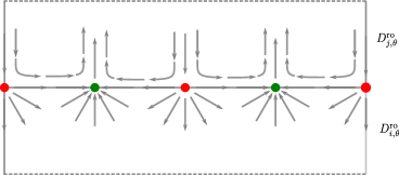
Figure 8.2.1: Trajectories of the scaled vector field along the boundary, near the corner locus. The winding number on $D^{\mathrm{ro}}_{j,\theta}$ around the boundary component seen here, is computed by a path going from left to right in the upper half of the figure, and so coincides with the number of red (or green) points. On $D^{\mathrm{ro}}_{i,\theta}$ we find the same number with the opposite sign.

Notation 8.2.10.

Take a connected component of some $D^{\mathrm{ro}}_{i,j,\theta}$ with $\varpi_{i}$ or $\varpi_{j}$ not zero and such that $j\to i$. A point of $\Sigma_{i,j}^{+}$ will be called a red point, that is, a red point looks like half a fountain on $D^{\mathrm{ro}}_{i,\theta}$ and half a saddle point on $D^{\mathrm{ro}}_{j,\theta}$. Analogously, a point of $\Sigma_{i,j}^{-}$ will be called a green point, that is, a green point looks like half a sink on $D^{\mathrm{ro}}_{i,\theta}$ and half a saddle point on $D^{\mathrm{ro}}_{j,\theta}$. See fig. 8.2.1 for a drawing of the vector field $\xi^{\mathrm{ro}}_{i,j,\theta}$.

8.3 The strict transform

In this subsection we rescale the pull-back $\pi_{\mathrm{pol}}^{*}\xi$ in a neighborhood of a component $D_{a}$ of the strict transform $C_{\mathrm{pol}}$, for some $a\in\mathcal{A}$. With the right rescaling, this vector field looks like a Morse-Bott attractor along $D_{a}$. As a result, the flow of the vector field retracts a neighborhood onto $D_{a}$, and, as we shall see, the strict transform $\overline{\pi_{\mathrm{pol}}^{-1}(S\setminus\{0\}}\subset Y_{\mathrm{pol}}$ of the total spine does not intersect a neighborhood of $C_{\mathrm{pol}}$.

8.3.1.

Let $a\in\mathcal{A}$ be an arrowhead in the graph $\Gamma_{\mathrm{pol}}$, and let $i\in\mathcal{V}$ be the unique neighbor of $a$ in $\Gamma_{\mathrm{pol}}$. Then $D_{i}$ is an exceptional component, and $D_{a}$ is a component of the strict transform $C_{\mathrm{pol}}\subset Y_{\mathrm{pol}}$. These divisors intersect in a unique point, choose a small coordinate chart $U$ around this point. We can assume that the coordinates $u,v$ in $U$ satisfy

$$\pi^{*}x|_{U}=u^{c_{0,i}},\qquad\pi^{*}f|_{U}=u^{m_{i}}v^{a_{i}}.$$

Since $\pi_{\mathrm{pol}}$ restricts to an isomorphism outside the exceptional divisor, and $\xi$ is a well defined vector field outside the curve $C$, we have a well defined vector field $\pi_{\mathrm{pol}}^{*}\xi$ on the set $U\setminus D=U\setminus(D_{i}\cup D_{a})$.

After choosing a small neighborhood $U$, we can choose $\varepsilon$ and $\eta$ small enough that we can assume that $D_{a}\cap\pi_{\mathrm{pol}}^{-1}({\mathrm{Tub}}(\varepsilon,\eta))\subset U$.

Lemma 8.3.2.

The vector field

(8.3.3) $$|u|^{\tau_{i}}|v|^{2}\cdot\pi_{\mathrm{pol}}^{*}\xi|_{U\setminus D}$$

extends to an analytic vector field on $U$. Furthermore,

1. the singular set of this extension is the submanifold $U\cap D_{a}$,

2. the Hessian of this extension has strictly negative real eigenvalues along the normal bundle of the singular set.

Proof.

By the definition of a pull-back of a vector field, we find

$$\pi_{\mathrm{pol}}^{*}\xi|_{U\setminus D}=\left(\begin{matrix}\xi^{u}\\ \xi^{v}\end{matrix}\right)=(\mathop{\mathrm{Jac}}\pi_{\mathrm{pol}})^{-1}\cdot\left(\begin{matrix}\bar{f}_{x}/\bar{f}\\ \bar{f}_{y}/\bar{f}\end{matrix}\right)=\mathop{\mathrm{Jac}}\pi_{\mathrm{pol}}^{-1}(\mathop{\mathrm{Jac}}\pi_{\mathrm{pol}}^{-1})^{*}\cdot\left(\begin{matrix}m_{i}\bar{u}^{-1}\\ a_{i}\bar{v}^{-1}\end{matrix}\right)$$

Here we use the assumption that $f=u^{m_{i}}v^{a_{i}}$ is a monomial, and so its log derivatives are easily computed:

$$f_{u}/f=m_{i}u^{-1},\qquad f_{v}/f=a_{i}v^{-1}.$$

A computation gives (note that $x_{v}=0$ and so $\det\mathop{\mathrm{Jac}}\pi_{\mathrm{pol}}=x_{u}y_{v}$)

$$\mathop{\mathrm{Jac}}\pi_{\mathrm{pol}}^{-1}(\mathop{\mathrm{Jac}}\pi_{\mathrm{pol}}^{-1})^{*}=\dfrac{1}{|x_{u}y_{v}|^{2}}\left(\begin{matrix}|y_{v}|^{2}&-y_{v}\bar{y}_{u}\\ -y_{u}\bar{y}_{v}&|x_{u}|^{2}+|y_{u}|^{2}\end{matrix}\right)=\dfrac{1}{|y_{v}|^{2}}\left(\begin{matrix}\left|\dfrac{y_{v}}{x_{u}}\right|^{2}&-\dfrac{y_{v}}{x_{u}}\dfrac{\bar{y}_{u}}{\bar{x}_{u}}\\[11.00008pt] -\dfrac{y_{u}}{x_{u}}\dfrac{\bar{y}_{v}}{\bar{x}_{u}}&1+|\dfrac{y_{u}}{x_{u}}|^{2}\end{matrix}\right).$$

As a result, since $\tau_{i}=2c_{1,i}$, we find

(8.3.4) $$|u|^{\tau_{i}}|v|^{2}\pi_{\mathrm{pol}}^{*}\xi=v\cdot\left|\frac{u^{c_{1,i}}}{y_{v}}\right|^{2}\cdot\left(\begin{matrix}-m_{i}\dfrac{\bar{v}}{\bar{u}}\left|\dfrac{y_{v}}{x_{u}}\right|^{2}+m_{a}\dfrac{y_{v}}{x_{u}}\dfrac{\bar{y}_{u}}{\bar{x}_{u}}\\[11.00008pt] m_{i}\dfrac{\bar{v}}{\bar{u}}\dfrac{y_{u}}{x_{u}}\dfrac{\bar{y}_{v}}{\bar{x}_{u}}-m_{a}-m_{a}\left|\dfrac{y_{u}}{x_{u}}\right|^{2}\end{matrix}\right).$$

Here, the factor $\left|\frac{u^{c_{1,i}}}{y_{v}}\right|^{2}$ is a positive unit, since $y_{v}$ vanishes with order $c_{1,i}$ along $D_{i}$ (see 3.3.4). In fact, since $y_{v}$ and $y_{u}$ both vanish with order strictly higher than $x_{u}$, all the summands in each coordinates of the vector to the right in eq. 8.3.4 are real analytic functions. As a result, eq. 8.3.3 has a real analytic extension. The factor $v$ in eq. 8.3.4 guarantees that the extension vanishes along $D_{i}$. In fact, the extension of both functions

$$|u|^{\tau_{i}}|v|^{2}\xi^{u},\qquad|u|^{\tau_{i}}|v|^{2}\xi^{v}$$

vanish along $D_{a}$, and the latter has the linear term $v$ with coefficient given by

$$-m_{a}-m_{a}\left|\frac{y_{u}}{x_{u}}\right|^{2}<0$$

at each point in $D_{a}$. It follows that the extension of eq. 8.3.3 vanishes precisely along $D_{a}$, and that the Hessian has negative eigenvalues along the normal bundle. ∎

Lemma 8.3.5.

Let $U^{\mathrm{ro}}=\sigma^{-1}(U)\subset Y^{\mathrm{ro}}_{\mathrm{pol}}$ with polar coordinates $(r,s,\alpha,\beta)$ so that $u=re^{i\alpha}$ and $v=se^{i\beta}$. The vector field

(8.3.6) $$r^{\tau}_{i}s(\pi^{\mathrm{ro}}_{\mathrm{pol}})^{*}\xi,$$

which is well defined on $U^{\mathrm{ro}}\setminus\partial U^{\mathrm{ro}}$, extends to a real analytic vector field on $U^{\mathrm{ro}}$ which does not vanish on $U^{\mathrm{ro}}$ and is tangent to $D^{\mathrm{ro}}_{i}$ and is transverse to $D^{\mathrm{ro}}_{a}$, pointing outwards there.

Proof.

The vector field

$$(\pi^{\mathrm{ro}}_{\mathrm{pol}})^{*}\xi|_{U^{\mathrm{ro}}\setminus\partial U^{\mathrm{ro}}}=\left(\begin{matrix}\xi^{\mathrm{ro},r}\\ \xi^{\mathrm{ro},\alpha}\\ \xi^{\mathrm{ro},s}\\ \xi^{\mathrm{ro},\beta}\end{matrix}\right)$$

is the pull-back of $\pi_{\mathrm{pol}}^{*}\xi|_{U\setminus D}$ to $U^{\mathrm{ro}}\setminus\partial U^{\mathrm{ro}}$, where the coordinates are given by eq. 8.1.3. Since $\xi_{U}$ is tangent to $D_{i}$, the analytic function $|u|^{\tau_{i}}|v|^{2}\xi^{u}$ is divisible by $u$. Furthermore, by eq. 8.3.4, $|u|^{\tau_{i}}|v|^{2}\xi^{u}$ is also divisible by $v$. As a result, $\sigma^{*}(|u|^{\tau_{i}}|v|^{2}\xi^{u})$ is divisible by both $r$ and $s$, and so the functions

$$\begin{split}r^{\tau_{i}}s\xi^{\mathrm{ro},r}&=s^{-1}\mathop{\mathrm{Re}}(e^{-i\alpha}\sigma^{*}(|u|^{\tau_{i}}|v|^{2}\xi^{u}))\\ r^{\tau_{i}}s\xi^{\mathrm{ro},\alpha}&=s^{-1}r^{-1}\mathop{\mathrm{Im}}(e^{-i\alpha}\sigma^{*}(|u|^{\tau_{i}}|v|^{2}\xi^{u}))\end{split}$$

extend to real analytic functions on $U^{\mathrm{ro}}$. Similarly, we have

$$\begin{split}r^{\tau_{i}}s\xi^{\mathrm{ro},s}&=s^{-1}\mathop{\mathrm{Re}}(e^{-i\alpha}\sigma^{*}(|u|^{\tau_{i}}|v|^{2}\xi^{v}))\\ r^{\tau_{i}}s\xi^{\mathrm{ro},\beta}&=s^{-2}\mathop{\mathrm{Im}}(e^{-i\alpha}\sigma^{*}(|u|^{\tau_{i}}|v|^{2}\xi^{v}))\end{split}$$

The analytic function $|u|^{\tau_{i}}|v|^{2}\xi^{v}$ is divisible by $v$, and so $\mathop{\mathrm{Re}}(e^{-i\alpha}\sigma^{*}(|u|^{\tau_{i}}|v|^{2})\xi^{v})$ is divisible by $s$. As a result, $r^{\tau_{i}}s\xi^{\mathrm{ro},s}$ extends as an analytic function.

In a similar way, the function $\mathop{\mathrm{Im}}(e^{-i\alpha}\sigma^{*}(|u|^{\tau_{i}}|v|^{2}\xi^{v}))$ is divisible by $s$. But the only term in the expansion of $|u|^{\tau_{i}}|v|^{2}\xi^{v}$ which has order $1$ in $v$ is a real multiple of the variable $v$, it follows that $\mathop{\mathrm{Im}}(e^{-i\alpha}\sigma^{*}(|u|^{\tau_{i}}|v|^{2}\xi^{v}))$ is divisible by $s^{2}$. As a result, $r^{\tau_{i}}s\xi^{\mathrm{ro},\beta}$ has an analytic extension to $U^{\mathrm{ro}}$.

We have seen that the function $r^{\tau_{i}}s\xi^{\mathrm{ro},r}$ is divisible by $r$, and so vanishes along the boundary piece $D^{\mathrm{ro}}_{i}\cap U^{\mathrm{ro}}$. As a result, the vector field $r^{\tau_{i}}s(\pi^{\mathrm{ro}}_{\mathrm{pol}})^{*}\xi$ is tangent to $D^{\mathrm{ro}}_{i}\cap U^{\mathrm{ro}}$.

Similarly, since $\xi^{v}$ has linear part which is a negative multiple of $v$, the function

$$r^{\tau_{i}}s\xi^{\mathrm{ro},s}=s^{-1}\mathop{\mathrm{Re}}(e^{-i\alpha}\sigma^{*}(|u|^{\tau_{i}}|v|^{2}\xi^{v}))$$

takes negative values along the set defined by $s=0$. This means that the extension of $r^{\tau_{i}}s(\pi^{\mathrm{ro}}_{\mathrm{pol}})^{*}\xi$ is transverse to the boundary piece $D^{\mathrm{ro}}_{a}$. ∎

Definition 8.3.7.

With $U$ as in 8.3.1, and $U^{\mathrm{ro}}=\sigma^{-1}(U)$, denote by

$$\xi_{U},\qquad\xi^{\mathrm{ro}}_{U}$$

the unique extensions of the vector fields eq. 8.3.3 and eq. 8.3.6 to $U$ and $U^{\mathrm{ro}}$, respectively.

8.3.8.

For $p\in U$, denote by $\gamma_{p}$ the trajectory of $\xi_{U}$ starting at $p$. If $p\in U\setminus D$, then $\gamma_{p}$ is, up to reparametrization, the trajectory of $\xi$ pulled back to $U$ via $\pi_{\mathrm{pol}}$.

Corollary 8.3.9.

Let $U$ be as in 8.3.1. Then, there exists a smaller neighborhood $V\subset U$ satisfying

1. if $p\in V$, then $\gamma_{p}$ does not escape $U$,

2. if $p\in V\cap D_{i}$, then $\gamma_{p}$ converges to the unique intersection point in $D_{i}\cap D_{a}$,

3. if $p\in V\setminus D_{i}$, then $\gamma_{p}$ converges to a point in $D_{a}\setminus D_{i}$. ∎

Corollary 8.3.10.

There exists an open set $V\subset Y_{\mathrm{pol}}$ containing $C_{\mathrm{pol}}$ such that

$$\overline{\pi_{\mathrm{pol}}^{-1}(S)\setminus\{0\}}\cap V=\emptyset.\qed$$

8.4 Poincaré-Hopf indices

If $ij$ is an invariant vertex, then the vector field $\xi_{U}$ is tangent to the disks $D_{i}\cap U$ and $D_{j}\cap U$, and does not vanish outside the intersection point. As a result, restricting the vector field to either disk produces an index, see Definition 2.4.5.

Lemma 8.4.1.

1. Assume that $ij$ is an invariant edge. Then the restriction of $\xi_{U}|_{D_{i}\cap U}$ has an isolated singularity at $D_{i}\cap D_{j}$ of index one.

2. The set $D^{\mathrm{ro},\circ}_{i,\theta}\cap U^{\mathrm{ro}}$ consists of $\gcd(m_{i},m_{j})$ punctured disks. At each puncture, the restriction of $\xi^{\mathrm{ro}}_{U}$ has index

   $$\frac{1}{\gcd(m_{i},m_{j})}\left|\begin{matrix}\varpi_{i}&m_{0,i}\\ \varpi_{j}&m_{0,j}\\ \end{matrix}\right|+1.$$

3. The set $D^{\mathrm{ro},\circ}_{j,\theta}\cap U^{\mathrm{ro}}$ consists of $\gcd(m_{i},m_{j})$ punctured disks. On each disk, the restriction of $\xi^{\mathrm{ro}}_{U}$ has index

   $$\frac{-1}{\gcd(m_{i},m_{j})}\left|\begin{matrix}\varpi_{i}&m_{0,i}\\ \varpi_{j}&m_{0,j}\\ \end{matrix}\right|+1.$$

Proof.

For item (i), the Hessian of the restriction has two equal real nonzero eigenvalues. As a result, it is, up to a coordinate change, a real scalar of the radial vector field, which has index $1$.

For item (ii) and item (iii), it suffices to have a look at fig. 8.2.1, and use eq. 2.4.6. Indeed, observe that, by Lemma 8.2.4, ii and iii, the number of red points is

(8.4.2) $$\frac{1}{\gcd(m_{i},m_{j})}\left|\begin{matrix}\varpi_{i}&m_{0,i}\\ \varpi_{j}&m_{0,j}\\ \end{matrix}\right|.$$

Which is the same as the number of green points. After contracting each connected component of $D^{\mathrm{ro}}_{i,j,\theta}$ to a point, we get a eq. 8.4.2-pronged singularity on $D^{\mathrm{ro}}_{j,\theta}$ and a eq. 8.4.2-petal singularity on $D^{\mathrm{ro}}_{i,\theta}$. So the result follows after Example 2.4.7. ∎

Lemma 8.4.3.

Assume that $ik$ is an edge from $i$ to $k$, and that $i$ is invariant and $k$ not invariant. Then the Poincaré-Hopf index of the vector field $\xi_{i}$ at the intersection point $D_{i}\cap D_{k}$ equals $1-\varpi_{k}$.

Proof.

Consider the the vector field $\xi^{\mathrm{ro}}_{i,j,\theta}|_{D^{\mathrm{ro}}_{i,\theta}}$. Let $L$ be one of the boundary components which is contained in $D^{\mathrm{ro}}_{i,j,\theta}$. Then, by Lemma 8.2.6 and Lemma 8.2.4 iii, the boundary component $L$ has $\varpi_{k}m_{i}/\gcd(m_{i},m_{k})$ red vertices. So, after contracting $L$ to a point, the vector field $\xi^{\mathrm{ro}}_{i,j,\theta}|_{D^{\mathrm{ro}}_{i,\theta}}$ has a $\varpi_{k}m_{i}/\gcd(m_{i},m_{k})$-pronged singularity. Now recall that for an invariant vertex $i$, the vector field $\xi^{\mathrm{ro}}_{i,\theta}$ is just the pullback by $\sigma$ of $\xi_{i}$ restricted to $D^{\mathrm{ro}}_{i,\theta}$. Furthermore, the map $\sigma|_{D^{\mathrm{ro}}_{i,\theta}}:D^{\mathrm{ro}}_{i,\theta}\to D_{i}$ is an $m_{i}$ regular cover, and, restricted to each component of $D^{\mathrm{ro}}_{i,\theta}$ is an $m_{i}/\gcd(m_{i},m_{j})$ regular cover. We find that $\xi_{i}$ has at $D_{i}\cap D_{k}$ a $\varpi_{k}$-pronged singularity. So, after Example 2.4.7, eq. 2.4.8, it has Poincaré-Hopf index $1-\varpi_{k}$. ∎

9 Other exceptional divisors

In this section, we consider an embedded resolution $\pi_{\mathrm{pol}}:Y_{\mathrm{pol}}\to\mathbb{C}^{2}$ (Definition 5.1.2) of the curve $(C,0)$ that resolves the generic polar curves, and fix a vertex $i\in\mathcal{V}$, which does not correspond to the first blow-up, $i\neq 0$. It may be impossible to scale and extend the vector field $\xi$ over the exceptional divisor $D_{i}$, to get a vector field on $D_{i}^{\circ}$, similar to $\xi_{0}$. In terms of numerical invariants on the graph, we characterize those divisors having such an extension. Furthermore, we describe a similar construction on the real oriented blow-up $Y^{\mathrm{ro}}$, which can be done for any exceptional divisor.

Notation 9.0.1.

We fix a metric induced by a coordinate change in $G_{\mathrm{pol}}$ (Definition 5.1.9). Fix also isometric coordinates (recall Definition 2.3.1) $x,y$ in $\mathbb{C}^{2}$ with respect to this metric chosen also so that the line $\{y=0\}$ is the tangent to $i$. This can always be achieved by a further unitary change of coordinates.

We usually simplify the notation by identifying functions defined in a neighborhood of the origin in $\mathbb{C}^{2}$ with their pullback to $U$ via $\pi_{\mathrm{pol}}$ or $U^{\mathrm{ro}}$ via $\pi^{\mathrm{ro}}_{\mathrm{pol}}$. That is, we sometimes write simply $f$ and $f_{x}$ instead of $\pi_{\mathrm{pol}}^{*}f$ and $f_{x}$, etc. Furthermore, the partials of $x=\pi_{\mathrm{pol}}^{*}x$ with respect to $u,v$ are denoted $x_{u},x_{v}$, and so on.

As in Section 4, we have the real oriented blow-up $\sigma:Y^{\mathrm{ro}}_{\mathrm{pol}}\to Y_{\mathrm{pol}}$, and the chart $U$ induces the chart $U^{\mathrm{ro}}=\sigma^{-1}(U)$ with coordinates $r=|u|$, $\alpha=\arg(u)$ and $v$. The boundary of $U^{\mathrm{ro}}$ is $\partial U^{\mathrm{ro}}=(\pi^{\mathrm{ro}}_{\mathrm{pol}})^{-1}(D_{i})$, given by $r=0$.

We choose a point $p\in D_{i}^{\circ}$, and a coordinate neighborhood $U$ containing $p$ so that $u(p)=v(p)=0$. Since $x$ vanishes with order $c_{0,i}$ along $D_{i}$, and does not vanish on $U\setminus D_{i}$, we can choose the coordinates $u,v$ so that

$$x=u^{c_{0,i}}.$$

Since the restriction $\pi_{\mathrm{pol}}|_{U\setminus D}:U\setminus D\to\mathbb{C}^{2}\setminus\{0\}$ is a local diffeomorphism, we can pull back $\xi$ to get $\pi_{\mathrm{pol}}|_{U\setminus D}^{*}\xi$.

In coordinates, we have complex functions $\xi^{u},\xi^{v}$ on $U\setminus D$ so that this vector field is given by the vector

(9.0.2) $$\pi_{\mathrm{pol}}|_{U\setminus D}^{*}\xi=\left(\begin{matrix}\xi^{u}\\ \xi^{v}\end{matrix}\right)=\frac{-1}{\det\mathop{\mathrm{Jac}}\pi\bar{f}}\left(\begin{matrix}y_{v}\bar{f}_{x}-x_{v}\bar{f}_{y}\\ -y_{u}\bar{f}_{x}+x_{u}\bar{f}_{y}\end{matrix}\right).$$

Similarly, on $U^{\mathrm{ro}}\setminus\partial U^{\mathrm{ro}}$, we have a vector field

$$\left.\pi^{\mathrm{ro}}_{\mathrm{pol}}\middle|_{U^{\mathrm{ro}}\setminus\partial U^{\mathrm{ro}}}^{*}\xi\right.=\left(\begin{matrix}\xi^{\mathrm{ro},r}\\ \xi^{\mathrm{ro},\alpha}\\ \xi^{\mathrm{ro},v}\end{matrix}\right)$$

Here, $\xi^{\mathrm{ro},r}$ and $\xi^{\mathrm{ro},\alpha}$ are real analytic functions, while $\xi^{\mathrm{ro},v}$ is, as before, a real analytic complex-valued function. We write $v=s+it$ an correspondingly $\xi^{\mathrm{ro},v}=\xi^{\mathrm{ro},s}+i\xi^{\mathrm{ro},t}$. Recall, 8.1.2, that a computation in polar coordinates gives

(9.0.3) $$\xi^{\mathrm{ro},v}=\sigma^{*}\xi^{v},\qquad\xi^{\mathrm{ro},r}=\mathop{\mathrm{Re}}\left(e^{-i\alpha}\sigma^{*}\xi^{u}\right),\qquad\xi^{\mathrm{ro},\alpha}=\mathop{\mathrm{Im}}\left((re^{i\alpha})^{-1}\sigma^{*}\xi^{u}\right).$$

Definition 9.0.4.

Let $P_{i}$ be the relative polar curve defined by the partial $f_{y}$, and denote by $\tilde{P}_{i}$ its strict transform by $\pi_{\mathrm{pol}}$.

Definition 9.0.5.

Let $i\in\mathcal{V}$ with $i\neq 0$. Set

$$\Sigma_{i}=\tilde{P}_{i}\cap D_{i}^{\circ},\qquad\Sigma^{\mathrm{ro}}_{i}=\sigma^{-1}(\Sigma_{i}),\qquad\Sigma^{\mathrm{ro}}_{i,\theta}=\Sigma^{\mathrm{ro}}\cap D_{i,\theta}^{\circ}.$$

and

$$\Sigma_{U}=\Sigma_{i}\cap U,\qquad\Sigma^{\mathrm{ro}}_{U}=\Sigma^{\mathrm{ro}}\cap U^{\mathrm{ro}}.$$

Note that we have a precise choice for the polar curve $P_{i}$, which depends on the metric and the vertex $i$. More precisely, $P_{i}$ is the vanishing set of the partial derivative of $f$ with respect to the direction orthogonal to the tangent associated with $i$. Therefore, even if we fix the underlying metric, the definition of $\Sigma_{i}$ for different vertices $i$ involves a different choice of the polar curve.

In contrast, $\Sigma_{0}$ cannot be seen as the intersection of $D_{0}^{\circ}$ with the strict transform of a particular polar curve. A signed count of singularities of the vector field $\xi_{0}$, however, allows for estimating the number of points in $\Sigma_{0}$ as the following lemma shows:

Lemma 9.0.6.

Let $F_{0}$ and $S_{0}$ be the number of fountains and saddle points, respectively, of $\xi_{0}$. If $t$ is the number of tangents of $C$, then

$$F_{0}-S_{0}=2-t$$

Proof.

By Lemma 7.4.13, the index of $\xi_{0}$ near $D_{0}\cap\tilde{C}$ is $1$. The Euler characteristic of $D_{0}$ is $2$. A direct application of Poincaré-Hopf index theorem yields the result. ∎

Remark 9.0.7.

The intersection $\Sigma_{i}$ consists of finitely many points. The preimage $\Sigma^{\mathrm{ro}}_{i}$ is therefore the union of finitely many fibers of the $S^{1}$-bundle $D^{\mathrm{ro},\circ}_{i}\to D^{\circ}_{i}$. These fibers are transverse to the foliation on $D^{\mathrm{ro},\circ}_{i}$ given by $\arg(f)$, whose leaves are $D^{\mathrm{ro},\circ}_{i,\theta}$ for $\theta\in\mathbb{R}/2\pi\mathbb{Z}$. In fact, $|\Sigma^{\mathrm{ro}}_{i,\theta}|=m_{i}\cdot|\Sigma_{i}|<\infty$.

9.1 Extension over the boundary

Lemma 9.1.1.

We use Notation 9.0.1.

• The vector field

  (9.1.2) $$r^{\tau_{i}}\pi^{\mathrm{ro}}_{\mathrm{pol}}|_{U^{\mathrm{ro}}\setminus\partial U^{\mathrm{ro}}}^{*}\xi$$

  on $U^{\mathrm{ro}}\setminus\partial U^{\mathrm{ro}}$ extends to an analytic vector field on $U^{\mathrm{ro}}$ which is tangent to $\partial U^{\mathrm{ro}}$ and whose vanishing set is $\Sigma^{\mathrm{ro}}_{U}$.

• If $i$ is an invariant vertex, that is, if $m_{i}-p_{i}=c_{1,i}$, then the vector field

  (9.1.3) $$|u|^{2c_{1,i}}\pi_{\mathrm{pol}}|_{U\setminus D}^{*}\xi=|u|^{\tau_{i}}\pi_{\mathrm{pol}}|_{U\setminus D}^{*}\xi$$

  on $U\setminus D$ extends to an analytic vector field on $U$, which is tangent to $D\cap U$ and whose vanishing set is $\Sigma_{U}$.

Proof.

Since $x=u^{c_{0,i}}$, we have $x_{v}=0$. As a result

$$r^{\tau_{i}}\xi^{u}=r^{c_{1,i}+m_{i}-p_{i}}\frac{-y_{v}\bar{f}_{x}}{\det\mathop{\mathrm{Jac}}\pi_{\mathrm{pol}}\bar{f}}=r^{c_{0,i}+c_{1,i}-1}r^{c_{0,i}-1}\frac{-y_{v}}{\det\mathop{\mathrm{Jac}}\pi_{\mathrm{pol}}}r^{m_{i}-p_{i}}\frac{\bar{f}_{x}}{\bar{f}}$$

The second factor $r^{c_{0,i}-1}\frac{-y_{v}}{\det\mathop{\mathrm{Jac}}\pi_{\mathrm{pol}}}$ extends over the boundary by Lemma 4.1.2. This is because by 3.3.4 we have $\mathrm{ord}_{u}y_{v}=c_{1,i}$ and $\mathrm{ord}_{u}\det\mathop{\mathrm{Jac}}\pi_{\mathrm{pol}}=\nu_{i}-1=c_{0,i}+c_{1,i}-1$. The third factor $r^{m_{i}-p_{i}}\frac{\bar{f}_{x}}{\bar{f}}$ also extends over the boundary since $\mathrm{ord}_{u}\bar{f}_{x}\geq p_{i}$ (eq. 5.1.6) and $\mathrm{ord}_{u}\bar{f}=m_{i}$. Finally, since $c_{1,i}-c_{0,i}+1\geq 2$ (because $i\neq 0$), the first factor $r^{c_{0,i}+c_{1,i}-1}$ vanishes identically along the boundary $\partial U^{\mathrm{ro}}$. We conclude, by the last two formulas of eq. 9.0.3 that both $r^{\tau_{i}}\xi^{\mathrm{ro},r}$ and $r^{\tau_{i}}\xi^{\mathrm{ro},\alpha}$ extend over and vanish along $\partial U^{\mathrm{ro}}$.

Similarly as above, again using Lemma 4.1.2, the function

(9.1.4) $$r^{c_{1,i}+m_{i}-p_{i}}\frac{x_{u}\bar{f}_{y}}{\det\mathop{\mathrm{Jac}}\pi\bar{f}}=r^{c_{1,i}}\frac{c_{0,i}u^{c_{0,i}-1}}{\det\mathop{\mathrm{Jac}}\pi}\cdot r^{m_{i}-p_{i}}\frac{\bar{f}_{y}}{\bar{f}}$$

extends to a real analytic $\cdot_{i}$-equivariant function of weight $c_{1,i}-m_{i}+p_{i}$ on $U^{\mathrm{ro}}$. We are using that $\mathrm{ord}_{u}\bar{f}_{y}=p_{i}$. Note that this function vanishes precisely along $\{r^{-p_{i}}f_{y}=0\}$ because

$$r^{c_{1,i}}\frac{c_{0,i}u^{c_{0,i}-1}}{\det\mathop{\mathrm{Jac}}\pi}\cdot r^{m_{i}}\frac{1}{\bar{f}}$$

is an unit. Also note that $\{r^{-p_{i}}f_{y}=0\}\cap\partial U^{\mathrm{ro}}=\tilde{P}_{i}\cap\partial U^{\mathrm{ro}}=\Sigma^{\mathrm{ro}}_{U}$.

By Lemma 3.5.2, and our choice of coordinates $x,y$, we have

$$\mathrm{ord}_{u}(y_{u})=\mathrm{ord}_{u}(y)-1>\mathrm{ord}_{u}(x)-1=\mathrm{ord}_{u}(x_{u}).$$

Furthermore, $\mathrm{ord}_{u}(f_{x})\geq\mathrm{ord}_{u}(f_{y})$ by eq. 5.1.6. Thus, as in the previous argument, the function

(9.1.5) $$r^{c_{1,i}+m_{i}-p_{i}}\frac{-y_{u}\bar{f}_{x}}{\det\mathop{\mathrm{Jac}}\pi\bar{f}}=r^{c_{1,i}}\frac{-y_{u}}{\det\mathop{\mathrm{Jac}}\pi}\cdot r^{m_{i}-p_{i}}\frac{\bar{f}_{x}}{\bar{f}}$$

on $U^{\mathrm{ro}}\setminus\partial U^{\mathrm{ro}}$ extends over the boundary and vanishes there.

By eq. 9.0.2 and eq. 9.0.3, the function $r^{\tau_{i}}\xi^{\mathrm{ro},v}$ is the sum of eq. 9.1.4 and eq. 9.1.5, and so extends to a function on $U^{\mathrm{ro}}$. Outside the boundary, the vector field $r^{\tau_{i}}\pi^{\mathrm{ro}}_{\mathrm{pol}}|_{U^{\mathrm{ro}}\setminus\partial U^{\mathrm{ro}}}^{*}\xi$ does not vanish since $\pi^{\mathrm{ro}}_{\mathrm{pol}}$ is a local diffeomorphism on $U^{\mathrm{ro}}\setminus\partial U^{\mathrm{ro}}$ and $\xi$ does not vanish outside the curve $C\subset\mathbb{C}^{2}$. Since the function in eq. 9.1.5 vanishes along $\partial U^{\mathrm{ro}}$, the vanishing set of $\xi^{\mathrm{ro},v}|_{\partial U^{\mathrm{ro}}}$ is that of the function in eq. 9.1.4 which we have already seen to be $\Sigma^{\mathrm{ro}}_{U}$. This finishes the proof of i.

ii follows from a completely analogous argument by replacing $r^{c_{1,i}+m_{i}-p_{i}}$ by $|u|^{2c_{1,i}}$. ∎

Lemma 9.1.6.

We use Notation 9.0.1.

• The vector field

  (9.1.7) $$\pi^{\mathrm{ro}}_{\mathrm{pol}}|_{Y^{\mathrm{ro}}\setminus D^{\mathrm{ro}}}^{*}(|x|^{\tau_{i}/c_{0,i}}\xi)$$

  on $Y^{\mathrm{ro}}\setminus D^{\mathrm{ro}}$ extends to an analytic vector field on $(Y^{\mathrm{ro}}\setminus D^{\mathrm{ro}})\cup D^{\mathrm{ro},\circ}_{i}$ which is tangent to $D^{\mathrm{ro},\circ}_{i}$ and whose vanishing set is $\Sigma^{\mathrm{ro}}_{i}$. Moreover, for each $\theta\in\mathbb{R}/2\pi\mathbb{Z}$, the extension is tangent to $D^{\mathrm{ro},\circ}_{i,\theta}$.

• If $i$ is an invariant vertex, that is, if $m_{i}-p_{i}=c_{1,i}$, then the vector field

  (9.1.8) $$\pi_{\mathrm{pol}}|_{Y\setminus D}^{*}(|x|^{2c_{1,i}/c_{0,i}}\xi)=\pi_{\mathrm{pol}}|_{Y\setminus D}^{*}(|x|^{\tau_{i}/c_{0,i}}\xi)$$

  on $Y\setminus D$ extends to an analytic vector field on $(Y\setminus D)\cup D^{\circ}_{i}$, which is tangent to $D^{\circ}_{i}$ and whose vanishing set is $\Sigma_{i}$.

Proof.

It is always possible to cover $D^{\mathrm{ro},\circ}_{i}$ by charts $U^{\mathrm{ro}}$ with coordinates $r,\alpha,v$ as in Notation 9.0.1. In those coordinates, we have that

$${\pi^{\mathrm{ro}}_{\mathrm{pol}}}^{*}|x|^{\tau_{i}/c_{0,i}}=|r|^{c_{0,i}}.$$

Similarly, it is possible to cover $D^{\circ}_{i}$ by charts $U$ with coordinates $u,v$ such that

$${\pi_{\mathrm{pol}}}^{*}|x|^{\tau_{i}/c_{0,i}}=|u|^{c_{0,i}}.$$

Then, the proof follows from Lemma 9.1.1. ∎

Definition 9.1.9.

Denote by $\xi^{\mathrm{ro}}_{U}$ the analytic vector field on $U^{\mathrm{ro}}$ whose restriction to $U^{\mathrm{ro}}\setminus\partial U^{\mathrm{ro}}$ coincides with eq. 9.1.2. If $i$ is an invariant vertex then denote by $\xi_{U}$ the analytic vector field on $U$ whose restriction to $U\setminus D$ coincides with eq. 9.1.3.

Similarly, denote by $\hat{\xi}^{\mathrm{ro}}_{i}$ the analytic vector field on $(Y\setminus D^{\mathrm{ro}})\cup D^{\mathrm{ro},\circ}_{i}$ whose restriction to $Y^{\mathrm{ro}}\setminus D^{\mathrm{ro}}$ coincides with eq. 9.1.7. If $i$ is an invariant vertex then denote by $\hat{\xi}_{i}$ the analytic vector field on $(Y\setminus D)\cup D^{\circ}_{i}$ whose restriction to $Y\setminus D$ coincides with eq. 9.1.8. Denote the restriction by $\xi_{i}=\hat{\xi}_{i}|_{D_{i}^{\circ}}$.

Finally, denote the other corresponding restrictions by $\xi^{\mathrm{ro}}_{i}=\hat{\xi}^{\mathrm{ro}}_{i}|_{D^{\mathrm{ro},\circ}_{i}}$ and $\xi^{\mathrm{ro}}_{i,\theta}=\xi^{\mathrm{ro}}_{i}|_{D^{\mathrm{ro},\circ}_{i,\theta}}$.

Remark 9.1.10.

Let $i\in\mathcal{V}_{\Upsilon}\setminus\{0\}$. In local coordinates on $D_{i}$, the vector field $\xi_{i}$ is determined by the initial part of the pullback of the function $f_{y}$. If we start with a different metric, then the same construction gives a vector field which is a linear combination of the pullbacks of $f_{x}$ and $f_{y}$. Since $f_{x}$ vanishes with a higher order than $f_{y}$, by 6.4.15, this construction gives the same result up to a real scalar. Therefore, the vector fields $\xi_{i}$ and $\xi^{\mathrm{ro}}_{i}$ do not depend on the chosen metric, up to a positive scalar.

9.2 A potential for $\xi_{i}$ on invariant vertices

In this subsection, we consider an invariant vertex $i\in\mathcal{V}_{\mathrm{pol}}\setminus\{0\}$. We show that the vector field $\xi_{i}$, defined in the previous subsection, has a scalar potential with respect to the metric $g_{i}$, defined in Definition 4.3.1. An analogous statement for $\xi^{\mathrm{ro}}_{i,\theta}$, and its proof, can be found in the next subsection. We choose a coordinate chart around a point $p\in D_{i}^{\circ}$ as in 3.3.4, and set $U^{\mathrm{ro}}=\sigma^{-1}(U)$.

Let $i\in\mathcal{V}\setminus\{0\}$ be an invariant vertex. The function

(9.2.1) $$\pi^{*}\left(-\log\frac{|f|}{|x|^{m_{i}/c_{0,i}}}\right)$$

extends as an analytic function over $D_{i}^{\circ}$. In fact, in coordinates $u,v$ in $U$, satisfying $x=u^{c_{0,i}}$, the function $f$ is divisible by $u^{m_{i}}$, and $|x|^{m_{i}/c_{0,i}}=|u^{m_{i}}|$.

Definition 9.2.2.

Denote by $\phi_{i}:D_{i}^{\circ}\to\mathbb{R}$ the restriction of the extension of eq. 9.2.1 to $D_{i}^{\circ}$.

In coordinates $u,v$, we can write $\pi^{*}f=u^{m_{i}}g(v)+{\mathrm{h.o.t.}}$, where the higher order terms are divisible by $u^{m_{i}+1}$. Therefore, eq. 9.2.1 equals

$$\begin{split}-\log|f|+\log|u|^{m_{i}/c_{0,i}}&=-(\log|g(v)+{\mathrm{h.o.t.}}|+m_{i}\log|u|)+\log|u|^{m_{i}}\\ &=-\log|g(v)|\end{split}$$

along $D_{i}$, where $u$ vanishes. As a result,

(9.2.3) $$\phi_{i}(v)=-\log|g(v)|.$$

Lemma 9.2.4.

Let $i\neq 0$ be invariant vertex. The vector field $\xi_{i}$ is the gradient of $\phi_{i}$ with respect to the Riemannian metric $g_{i}$ from Definition 4.3.1.

Proof.

From eq. 9.0.2 and observing that $x_{v}=0$, we have the formula

(9.2.5) $$|u|^{\tau_{i}}\xi^{v}=|u|^{\tau_{i}}\frac{y_{u}\bar{f}_{x}-x_{u}\bar{f}_{y}}{x_{u}y_{v}\bar{f}}.$$

We recall from Definition 8.0.1 that $\tau_{i}=c_{1,i}+m_{i}-p_{i}$. Since $\varpi_{i}=0$ (recall Definition 6.1.1), we have that $\tau_{i}=2c_{1,i}$ and so

$$|u|^{\tau_{i}}=|u|^{2c_{1,i}}=u^{c_{1,i}}\bar{u}^{c_{1,i}}.$$

Similarly as in eq. 9.1.5, the term $|u|^{\tau_{i}}\frac{y_{u}\bar{f}_{x}}{x_{u}y_{v}\bar{f}}$ vanishes along $D_{i}^{\circ}$. The other term is

$$|u|^{2c_{1,i}}\frac{-x_{u}\bar{f}_{y}}{x_{u}y_{v}\bar{f}}=-\frac{|u|^{2c_{1,i}}\bar{f}_{y}}{y_{v}\bar{f}}=-\frac{|u|^{2c_{1,i}}\bar{f}_{v}}{|y_{v}|^{2}\bar{f}}.$$

In the last inequality we have used that $\bar{f}_{v}=\bar{y}_{v}\bar{f}_{y}$. Since $\varpi_{i}=0$, Lemma 6.1.3 implies that $\mathrm{ord}_{u}\bar{f}_{v}=\mathrm{ord}_{u}\bar{f}=m_{i}$. Therefore, we have $\mathop{\mathrm{in}}\nolimits_{u}f=u^{m_{i}}g(v)$ and $\mathop{\mathrm{in}}\nolimits_{u}f_{v}=u^{m_{i}}g^{\prime}(v)$. Along $D_{i}\cap U$, we find

$$\left.|u|^{\tau_{i}}\xi^{v}\right|_{D_{i}\cap U}=h^{-1}_{U}(v)\frac{g^{\prime}(\bar{v})}{g(\bar{v})}.$$

where $h_{U}$ is the real function defining the metric $g_{i}$, defined in Definition 4.3.1. The result now follows from Lemma 2.1.3, and 4.3.2. ∎

9.3 A potential for $\xi^{\mathrm{ro}}_{i,\theta}$

In this subsection, we fix a noninvariant vertex $i\in\mathcal{V}_{\mathrm{pol}}$, $\varpi_{i}\neq 0$, and a value $\theta\in\mathbb{R}/2\pi\mathbb{Z}$ of $\arg(f)$. We prove an analogous result to Lemmas 7.4.4 and 9.2.4 but for non-invariant vertices, that is, we show the existence of a potential function for the vector field $\xi^{\mathrm{ro}}_{i,\theta}$.

9.3.1.

Consider the Riemann surface $D^{\mathrm{ro},\circ}_{i,\theta}$, defined in Definition 4.2.1, with the metric $g^{\mathrm{ro}}_{i,\theta}$ defined in Definition 4.3.1. If we contract each boundary component of $D^{\mathrm{ro}}_{i,\theta}$ to a point, we get a branched covering over $D_{i}$. Thus, $D^{\mathrm{ro},\circ}_{i,\theta}$ is a Riemann surface with punctures. If $j\in\mathcal{V}_{\mathrm{pol}}$ is a neighbor of $i$, let $U\subset Y_{\mathrm{pol}}$ be a small coordinate chart containing the intersection $D_{i}\cap D_{j}$, and let $U^{\mathrm{ro}}=\sigma^{-1}(U)$. We can assume that $D_{i}\cap U$ is a disc. Thus, $D^{\mathrm{ro},\circ}_{i,\theta}\cap U^{\mathrm{ro}}$ covers a punctured disc, and so is a disjoint union of some number of punctured discs.

Lemma 9.3.2.

Let $D\subset D^{\mathrm{ro},\circ}_{i,\theta}$ be a connected component, and take $j\in\mathcal{V}_{\mathrm{pol}}$ so that $ji$ is the unique edge pointing to $i$. Let $U$ and $U^{\mathrm{ro}}$ be as in the previous paragraph. Then $D$ has genus zero, and $D\cap U^{\mathrm{ro}}$ is connected.

Proof.

It follows from Lemma 6.2.11item (ii) that the function $\arg(x)$ takes a constant value, say $\theta^{\prime}$, along $D$. Thus, $D$ is a connected component of the set $\arg(x)^{-1}(\theta^{\prime})\cap D^{\mathrm{ro},\circ}_{i}$. Thus, $D$ embeds into the Milnor fiber at radius zero of the function $x$. This Milnor fiber is a disk, and so $D$ has genus zero. The modification $Y_{\mathrm{pol}}\to\mathbb{C}^{2}$, and its real oriented blow-up, induce a decomposition of the Milnor fiber at radius zero (recall Definition 4.2.5) of $x$ of nested discs. Thus, each component has a unique outer boundary component. For the vertex $0$, this outer component is the boundary of the Milnor fiber, whereas for other vertices $i$, the outer component corresponding to the unique edge pointing to $i$. Since the closure of $D$ has a unique outer boundary component, the set $D\cap U^{\mathrm{ro}}$ is a single punctured disc, in particular, it is connected. ∎

Lemma 9.3.3.

Let $i$ be any vertex in $\mathcal{V}_{\mathrm{pol}}\setminus\{0\}$. Then, there exists a function $\phi^{\mathrm{ro}}_{i,\theta}:D^{\mathrm{ro},\circ}_{i,\theta}\to\mathbb{R}$ so that

$$\xi^{\mathrm{ro}}_{i,\theta}=\nabla\phi^{\mathrm{ro}}_{i,\theta}$$

where the gradient is taken with respect to the metric $g^{\mathrm{ro}}_{i,\theta}$ defined in Definition 4.3.1.

Furthermore, if $k$ is a neighbor of $i$ so that the edge $ik$ is oriented from $i$ to $k$, and $\varpi_{k}\neq 0$, then $\phi^{\mathrm{ro}}_{i,\theta}$ extends over the corresponding boundary components with constant value there.

Proof.

If $i$ is invariant, then we can take $\phi^{\mathrm{ro}}_{i,\theta}=\sigma^{*}\phi_{i}$, where $\phi_{i}:D_{i}\to\mathbb{R}$ is defined in the previous subsection. We leave the second statement for invariant vertices to the end of this proof.

So assume that $\varpi_{i}\neq 0$. By the previous lemma, $D^{\mathrm{ro},\circ}_{i,\theta}$ is a punctured sphere. To each neighbor of $i$, there corresponds a set of punctures. If $j$ is the unique neighbor of $i$ so that there is an edge from $j$ to $i$, then there is only one puncture corresponding to $j$ on each connected component. Let $D^{\mathrm{ro},{\scriptscriptstyle\cup}}_{i,\theta}$ be the Riemann surface obtained by filling in all the other punctures, thus, $D^{\mathrm{ro},{\scriptscriptstyle\cup}}_{i,\theta}$ is a disjoint union of copies of $\mathbb{C}$. Denote by $\kappa^{\mathrm{ro}}_{i,\theta}$ the differential form dual to $\xi^{\mathrm{ro}}_{i,\theta}$ with respect to the metric $g^{\mathrm{ro}}_{i,\theta}$. Let $u,v$ be a holomorphic coordinate system on a chart in $Y_{\mathrm{pol}}$, near a point $p\in D_{i}$ as before, and expand

$$f(u,v)=u^{m_{i}}f_{m_{i}}(v)+\ldots+u^{m_{i}+\varpi_{i}}f_{m_{i}+\varpi_{i}}+{\mathrm{h.o.t.}}$$

Then, by Lemma 6.1.3, we have

$$f^{\prime}_{m_{i}}=\ldots=f^{\prime}_{m_{i}+\varpi_{i}-1}=0,$$

and

$$f^{\prime}_{m_{i}+\varpi_{i}}\not\equiv 0.$$

As a result, we can write

$$\mathop{\mathrm{in}}\nolimits_{u}f=u^{m_{i}}f_{m_{i}}(v),\qquad\mathop{\mathrm{in}}\nolimits_{u}f_{v}=u^{m_{i}+\varpi_{i}}f^{\prime}_{m_{i}+\varpi_{i}}(v).$$

Similarly as in the proof of Lemma 9.1.1, the restriction of $|u|^{\tau_{i}}\xi^{v}$ to $\partial U^{\mathrm{ro}}$ is given by

$$|u|^{\tau_{i}}\frac{x_{u}\mathop{\mathrm{in}}\nolimits_{u}\bar{f}_{y}}{x_{u}y_{v}\mathop{\mathrm{in}}\nolimits_{u}\bar{f}}=|u|^{\tau_{i}}\frac{\mathop{\mathrm{in}}\nolimits_{u}\bar{f}_{v}}{|y_{v}|^{2}\mathop{\mathrm{in}}\nolimits_{u}\bar{f}}=\frac{|u|^{\tau_{i}}\bar{u}^{\varpi_{i}}}{|y_{v}|^{2}}\frac{\bar{f}^{\prime}_{m_{i}+\varpi_{i}}}{\bar{f}_{m_{i}}}=\left(\frac{u}{|u|}\right)^{-\varpi_{i}}\frac{|u|^{2c_{1,i}}}{|y_{v}|^{2}}\frac{\bar{f}^{\prime}_{m_{i}+\varpi_{i}}}{\bar{f}_{m_{i}}}.$$

Recall that the metric on $D^{\mathrm{ro},\circ}_{i,\theta}$ is given by the function

$$h_{U}(v)=\lim_{u\to 0}\frac{|y_{v}|}{|u|^{c_{1,i}}}.$$

Furthermore, the function $u/|u|$ is locally constant on $D^{\mathrm{ro},\circ}_{i,\theta}$ because of Lemma 6.1.3.

By 4.3.2, the differential form $\kappa^{\mathrm{ro}}_{i,\theta}$ is given, in the coordinate $v$, by the complex function

$$\left(\frac{u}{|u|}\right)^{-\varpi_{i}}\frac{\bar{f}^{\prime}_{m_{i}+\varpi_{i}}}{\bar{f}_{m_{i}}},$$

which is antiholomorphic on $D^{\mathrm{ro},\circ}_{i,\theta}$ for $\theta$ fixed. By the Cauchy-Riemann equations, the form $\kappa^{\mathrm{ro}}_{i,\theta}$ is closed.

Now, assume that $v$ is a holomorphic coordinate in a chart around a puncture, corresponding to a vertex $k$, so that the edge $ik$ is oriented from $i$ to $k$. Assume that the puncture is given by $v=0$. As a result, we can represent $\kappa^{\mathrm{ro}}_{i,\theta}$ by an antiholomorphic complex function $\alpha+i\beta$ on a punctured disk. Since

$$\lim_{v\to 0}|u|^{\tau_{i}}|v|^{\tau_{k}}\xi^{v}=0,$$

the function $|v|^{\tau_{k}}(\alpha+i\beta)$ is bounded on the punctured disk. It follows from the Riemann extension theorem that the holomorphic function $\alpha-i\beta$ has a meromorphic singularity at $v=0$.

As a result, the vanishing order of $\alpha-i\beta$ at $v=0$ is minus the Poincaré-Hopf index of $\xi^{\mathrm{ro}}_{i,\theta}$ at the puncture. By Lemma 8.4.1, this index is

$$\frac{-1}{\gcd(m_{i},m_{k})}\left|\begin{matrix}\varpi_{k}&m_{k}\\ \varpi_{i}&m_{i}\end{matrix}\right|+1.$$

By 6.3.7 and 6.3.6 item (v), the index is nonpositive, and so $\kappa^{\mathrm{ro}}_{i,\theta}$ does not have a pole at $v=0$. Therefore, $\kappa^{\mathrm{ro}}_{i,\theta}$ extends as a closed form on $D^{\mathrm{ro},{\scriptscriptstyle\cup}}_{i,\theta}$, which is a disjoint union of copies of $\mathbb{C}$. It follows that $\kappa^{\mathrm{ro}}_{i,\theta}$ is exact, i.e. there exists $\phi^{\mathrm{ro}}_{i,\theta}:D^{\mathrm{ro},\circ}_{i,\theta}\to\mathbb{R}$ with $\kappa^{\mathrm{ro}}_{i,\theta}=d\phi^{\mathrm{ro}}_{i,\theta}$, or equivalently, $\xi^{\mathrm{ro}}_{i,\theta}=\nabla\phi^{\mathrm{ro}}_{i,\theta}$. Furthermore, $\phi^{\mathrm{ro}}_{i,\theta}$ extends continuously over the punctures corresponding to the edge $ik$, and so, has a constant limit at each corresponding boundary component.

If $i$ is invariant, then the same argument as above applies to show that $\phi_{i}$ has a limit at a puncture corresponding to $ik$, if $i$ is such that $i\to k$, using, again, Lemma 8.4.1. This finishes the proof. ∎

10 Singularities on the boundary of $Y^{\mathrm{ro}}_{\mathrm{pol}}$

In this section we study the singularities of $\xi^{\mathrm{ro}}_{U}$ (Definition 9.1.9) on $\partial U^{\mathrm{ro}}$. Fix a point $p\in\Sigma_{i}$ with $i\neq 0$ and assume that the strict transform of $\{f_{y}=0\}$ defines the polar curve $P_{i}$ Definition 9.0.4. Since $\pi_{\mathrm{pol}}$ resolves the polar curve $P_{i}$ (Definition 9.0.4), the function $\pi_{\mathrm{pol}}^{*}f_{y}$ vanishes along a smooth curve $\tilde{P}_{i}$ passing through $p$ meeting $D_{i}^{\circ}$ transversely. As a consequence, on top of choosing $u$ so that $x=u^{c_{0,i}}$ as in Notation 9.0.1, we can choose $v$ so that

$$\pi_{\mathrm{pol}}^{*}f_{y}=u^{p_{i}}v.$$

10.1 Spinal cells

In this subsection we give name to the sets of trajectories of the vector field $\pi_{\mathrm{pol}}^{*}\xi$ that converge to points in the sets $\Sigma_{i}$.

Definition 10.1.1.

Let $i\in\mathcal{V}_{\mathrm{pol}}\setminus\{0\}$, let $p\in\Sigma_{i}$. We define the set

$$S(p)=\left\{b\in{\mathrm{Tub}}^{*}\,\middle|\,\text{the trajectory }(\pi_{\mathrm{pol}})^{*}\gamma_{b}\text{ converges to }p\text{ in }Y_{\mathrm{pol}}\right\}$$

Now fix $q\in\sigma^{-1}(p)$ and $\theta=\arg(q)$. We define the sets

$$S_{\theta}(p)=\left\{b\in{\mathrm{Tub}}_{\theta}^{*}\,\middle|\,\text{the trajectory }(\pi_{\mathrm{pol}})^{*}\gamma_{b}\text{ converges to }p\text{ in }Y_{\mathrm{pol},\theta}\right\}$$

and

$$S(q)=\left\{b\in{\mathrm{Tub}}^{*}\,\middle|\,\text{the trajectory }(\pi^{\mathrm{ro}}_{\mathrm{pol}})^{*}\gamma_{b}\text{ converges to }q\text{ in }Y^{\mathrm{ro}}_{\mathrm{pol},\theta}\right\}$$

Remark 10.1.2.

We describe a few easy properties of the sets defined above. Recall the definition of the total spine $S$ in Definition 2.2.4.

Let $p\in\Sigma_{i}$. We have the containments,

$$S(q)\subset S_{\theta}(p)\subset S(p)\subset S.$$

wit $\arg(q)=\theta$. Also, by definition

$$S(p)=\bigcup_{q\in\sigma^{-1}(p)}S(q)$$

and

$$S_{\theta}(p)=\bigcup_{\begin{subarray}{c}q\in\sigma^{-1}(p)\\ \arg(q)=\theta\end{subarray}}S(q).$$

Finally observe that $\sigma^{-1}(p)$ is a circle and that there are exactly $m_{i}$ points $q\in\sigma^{-1}(p)$ with $\arg(q)=\theta$ for each $\theta\in\mathbb{R}/2\pi\mathbb{Z}$.

All the sets in Definition 10.1.1 are contained, by definition, in ${\mathrm{Tub}}^{*}$. In the next definition we describe the counterpart of $S(q)$ in $Y^{\mathrm{ro}}_{\mathrm{pol}}$.

Definition 10.1.3.

For $q\in\Sigma^{\mathrm{ro}}_{i,\theta}$ we define the set

$$S^{\mathrm{ro}}(q)=\left\{a\in Y^{\mathrm{ro}}_{\mathrm{pol},\theta}\setminus\partial Y^{\mathrm{ro}}_{\mathrm{pol},\theta}\,\middle|\,\text{the trajectory }\gamma_{a}\text{ of }(\pi^{\mathrm{ro}}_{\mathrm{pol}})^{*}\xi\text{ converges to }q\text{ in }Y^{\mathrm{ro}}_{\mathrm{pol},\theta}\right\}.$$

Equivalently, $S^{\mathrm{ro}}(q)=(\pi^{\mathrm{ro}}_{\mathrm{pol}})^{-1}(S(q))$. Analogously, we define

$$S^{\mathrm{ro}}(p)=\left\{a\in Y^{\mathrm{ro}}_{\mathrm{pol}}\setminus\partial Y^{\mathrm{ro}}_{\mathrm{pol}}\,\middle|\,\text{the trajectory }(\pi_{\mathrm{pol}})^{*}\gamma_{b}\text{ converges to }p\text{ in }Y_{\mathrm{pol}}\right\},$$

or, equivalently, $S^{\mathrm{ro}}(p)=(\pi^{\mathrm{ro}}_{\mathrm{pol}})^{-1}(S(p))$.

Definition 10.1.4.

Given a coordinate chart $U$ around $p$ as in the previous sections, recall Definition 9.1.9. We define

$$S^{\mathrm{ro}}_{U}=\left\{a\in U^{\mathrm{ro}}\,\middle|\,\text{the trajectory }\gamma_{a}\text{ of }\xi^{\mathrm{ro}}_{U}\text{ converges to a point in }\sigma^{-1}(p)\text{ in }U^{\mathrm{ro}}\right\}.$$

The main goal of this section is to prove the following proposition. Its proof is relegated to Subsection 10.3 after enough theory is developed.

Proposition 10.1.5.

The set $S^{\mathrm{ro}}_{U}$ satisfies

1. It is a submanifold of $U^{\mathrm{ro}}$ of real dimension $3$ transverse to $\partial U^{\mathrm{ro}}$,

2. it contains $\sigma^{-1}(p)$, and

3. if $q\in\sigma^{-1}(p)$ then the tangent space $T_{q}S^{\mathrm{ro}}_{U}$ is the sum of the kernel and the negative eigenspace of ${\mathrm{Hess}}_{q}\xi^{\mathrm{ro}}_{U}$ (eq. 10.2.6), which is generated by the three vectors

   $$\partial_{r}+P\partial_{s}+Q\partial_{t},\qquad\partial_{\alpha},\qquad P^{\prime}\partial_{s}+Q^{\prime}\partial_{t},$$

   where $P+iQ=-\bar{\lambda}_{p}^{-1}e^{-i\varpi_{i}\alpha}\overline{\partial_{r}r^{\tau_{i}}\xi^{\mathrm{ro},v}(q)}$ and $P^{\prime}+iQ^{\prime}=\sqrt{-e^{-i\varpi_{i}\alpha}\lambda_{p}}$.

10.2 The Hessian in $U^{\mathrm{ro}}$

In this subsection we compute the Hessian of $\xi^{\mathrm{ro}}_{U}$ along its singular set $\sigma^{-1}(p)$, for some $p\in\Sigma_{i}$. This Hessian is block-triangular.

Definition 10.2.1.

For $\lambda\in\mathbb{C}$, define $2\times 2$ real matrices

$$A(\lambda)=\left(\begin{matrix}\mathop{\mathrm{Re}}(\lambda)&-\mathop{\mathrm{Im}}(\lambda)\\ \mathop{\mathrm{Im}}(\lambda)&\mathop{\mathrm{Re}}(\lambda)\\ \end{matrix}\right),\qquad\bar{A}(\lambda)=\left(\begin{matrix}\mathop{\mathrm{Re}}(\lambda)&\mathop{\mathrm{Im}}(\lambda)\\ \mathop{\mathrm{Im}}(\lambda)&-\mathop{\mathrm{Re}}(\lambda)\\ \end{matrix}\right).$$

Remark 10.2.2.

A direct computation yields

$$\bar{A}(\lambda)^{-1}=\frac{1}{|\lambda|^{2}}\bar{A}(\lambda).$$

Remark 10.2.3.

The matrices $A(\lambda)$, $\bar{A}(\lambda)$ describe real linear maps $\mathbb{C}\to\mathbb{C}$ which are either complex linear on antilinear. If $V\subset\mathbb{C}$ is an open set, and $h:V\to\mathbb{C}$ is differentiable, then the Jacobian of $h$ is given by the formula

$$\mathop{\mathrm{Jac}}h(v)=A(\partial_{v}h(v))+\bar{A}(\partial_{\bar{v}}h(v)).$$

If $\lambda\neq 0$, then the matrix $\bar{A}(\lambda)$ has eigenvectors $\sqrt{\lambda}$, with eigenvalue $|\lambda|>0$, and $\sqrt{-\lambda}$, with eigenvalue $-|\lambda|<0$. Furthermore, these two eigenspaces are orthogonal with respect to any inner product that is compatible with the complex structure of $\mathbb{C}$.

Lemma 10.2.4.

Let $V\subset\mathbb{C}$ be an open set, and $h,k:V\to\mathbb{C}$ differentiable functions. Assume that $h$ is antiholomorphic and vanishes at $p\in V$. Then the function $k\cdot h$, seen as a vector field on $V$, has an elementary singularity at $p$ whose Hessian is $\bar{A}(k(p)\cdot\partial_{\bar{v}}h(p))$.

Proof.

The lemma follows from Remark 10.2.3, since

$$\begin{split}\partial_{v}(h\cdot k)(p)&=\partial_{v}h(p)\cdot k(p)+h(p)\cdot\partial_{v}k(p)=0,\\ \partial_{\bar{v}}(h\cdot k)(p)&=\partial_{\bar{v}}h(p)\cdot k(p)+h(p)\cdot\partial_{\bar{v}}k(p)=k(p)\cdot\partial_{\bar{v}}h(p).\qed\end{split}$$

In this subsection we use real coordinates $r,\alpha,s,t$ for $U^{\mathrm{ro}}$ with $r,\alpha$ (the pullback of) polar coordinates for $u$ and $s+it=v$, and $u,v$ coordinates in $U$.

Lemma 10.2.5.

There exists a $\lambda_{p}\in\mathbb{C}^{*}$ so that if $q\in\sigma^{-1}(p)$, and we set $\alpha=\arg(u)(q)$. Then, the matrix ${\mathrm{Hess}}_{q}\xi^{\mathrm{ro}}_{U}$ expressed in $2\times 2$ blocks with respect to the coordinates $r,\alpha,s,t$, is

(10.2.6) $${\mathrm{Hess}}_{q}\xi^{\mathrm{ro}}_{U}=\left(\begin{matrix}\lx@intercol\hfil\hbox{\multirowsetup\scalebox{2.0}{$0$}}\hfil\lx@intercol&\lx@intercol\hfil\hbox{\multirowsetup\scalebox{2.0}{$0$}}\hfil\lx@intercol\\ \lx@intercol\hfil\hfil\lx@intercol&\lx@intercol\hfil\hfil\lx@intercol\\ (\partial_{r}\mathop{\mathrm{Re}}(r^{\tau_{i}}\xi^{\mathrm{ro},v}))|_{q}&0&\lx@intercol\hfil\hbox{\multirowsetup$\bar{A}(e^{-i\varpi_{i}\alpha}\lambda_{p})$}\hfil\lx@intercol\\ (\partial_{r}\mathop{\mathrm{Im}}(r^{\tau_{i}}\xi^{\mathrm{ro},v})|_{q}&0&\lx@intercol\hfil\hfil\lx@intercol\end{matrix}\right).$$

Proof.

We split the proof into three parts.

Part 1. In this first part we take care of the first $2$ rows of the matrix. In order to show that this $2\times 4$ matrix is null, it is enough to show that both $r^{\tau_{i}}\xi^{\mathrm{ro},r}$ and $r^{\tau_{i}}\xi^{\mathrm{ro},\alpha}$ are divisible by $r^{2}$, that is, in particular they are in the square of the maximal ideal of the local ring at $q$.

First we take care of $r^{\tau_{i}}\xi^{\mathrm{ro},r}$ which, by eq. 9.0.3, equals $r^{\tau_{i}}\mathop{\mathrm{Re}}(e^{-i\alpha}\sigma^{*}\xi^{u})$. Now, using eq. 9.0.2 and our choice of coordinates we find that

$$\mathrm{ord}_{u}(y_{v}\bar{f}_{x})>c_{0,i}+p_{i}.$$

Because $\mathrm{ord}_{u}(\bar{f}_{x})\geq\mathrm{ord}_{u}(\bar{f}_{y})$ by 5.1.6 and $\mathrm{ord}_{(}y_{v})=c_{1,i}>c_{0,i}$ by Lemma 3.5.2. On another hand, the order of vanishing of the denominator is

$$\mathrm{ord}_{u}(\det\mathop{\mathrm{Jac}}\pi_{\mathrm{pol}}\bar{f})=c_{0,i}+c_{1,i}-1+m_{i}.$$

Finally, taking into account the factor $r^{\tau_{i}}$, we estimate

$$\begin{split}\mathrm{ord}_{r}(r^{\tau_{i}}\xi^{\mathrm{ro},r})&=\tau_{i}+\mathrm{ord}_{r}(y_{v}\bar{f}_{x})-c_{0,i}-c_{1,i}+1-m_{i}\\ &>c_{1,i}+m_{i}-p_{i}+c_{0,i}+p_{i}-c_{0,i}-c_{1,i}+1-m_{i}\\ &=1.\end{split}$$

This implies that $r^{\tau_{i}}\xi^{\mathrm{ro},r}$ vanishes with order at least $2$ along the boundary.

Now we take care of $r^{\tau_{i}}\xi^{\mathrm{ro},\alpha}$. The argument for this part is more delicate. Notice that in the expression for $\xi^{\mathrm{ro},\alpha}$ in eq. 9.0.3 there is a factor $r^{-1}$ that was not present in the step before. In this case, a similar computation yields only the weaker inequality $\mathrm{ord}_{r}(r^{\tau_{i}}\xi^{\mathrm{ro},\alpha})\geq 1$. Next, we are going to argue that this function actually vanishes with order $2$ at $q$. If the above inequality is strict, there is nothing to prove. Assume otherwise that

(10.2.7) $$\mathrm{ord}_{r}(r^{\tau_{i}}\xi^{\mathrm{ro},\alpha})=1.$$

That is equivalent to saying that $\mathrm{ord}_{r}(r^{\tau_{i}}\xi^{u})=2$, which in turn, is equivalent to saying that

(10.2.8) $$\mathrm{ord}_{r}(y_{v}\bar{f}_{x})=c_{0,i}+1+p_{i}.$$

In general we know that $\mathrm{ord}_{r}(y_{v})\geq c_{0,i}+1$ and $\mathrm{ord}_{r}(\bar{f}_{x})\geq p_{i}$ so, in order to have eq. 10.2.8, we need these two inequalities to be equalities, that is:

$$c_{1,i}=\mathrm{ord}_{r}(y_{v})=c_{0,i}+1$$

and

$$\mathrm{ord}_{r}(\bar{f}_{x})=p_{i}$$

A computation gives (since $u_{v}=0$):

$$\left(\begin{matrix}f_{u}\\ f_{v}\end{matrix}\right)=\left(\begin{matrix}x_{u}&y_{u}\\ 0&y_{v}\end{matrix}\right)\left(\begin{matrix}f_{x}\\ f_{y}\end{matrix}\right),\quad\left(\begin{matrix}f_{x}\\ f_{y}\end{matrix}\right)=\frac{1}{x_{u}y_{v}}\left(\begin{matrix}y_{v}&-y_{u}\\ 0&x_{u}\end{matrix}\right)\left(\begin{matrix}f_{u}\\ f_{v}\end{matrix}\right)=\left(\begin{matrix}\frac{1}{x_{u}}f_{u}-\frac{y_{u}}{x_{u}y_{v}}f_{v}\\ \frac{1}{y_{v}}f_{v}\end{matrix}\right).$$

In particular, we use that $\det\mathop{\mathrm{Jac}}\pi_{\mathrm{pol}}=x_{u}y_{v}$, and so

(10.2.9) $$\xi^{u}=\frac{-y_{v}\bar{f}_{x}}{\det\mathop{\mathrm{Jac}}\pi_{\mathrm{pol}}\cdot\bar{f}}=-\frac{1}{|x_{u}|^{2}}\cdot\frac{\bar{f}_{u}}{\bar{f}}+\frac{\bar{y}_{u}}{|x_{u}|^{2}\bar{y}_{v}}\cdot\frac{\bar{f}_{v}}{\bar{f}}.$$

To compute the order of $\xi^{u}$, we find first

(10.2.10) $$\mathrm{ord}_{r}\left(-\frac{1}{|x_{u}|^{2}}\cdot\frac{\bar{f}_{u}}{\bar{f}}\right)=-2c_{0,i}+1,$$

since $\mathrm{ord}_{r}x_{u}=c_{0,i}-1$, and the logarithmic derivative of $f$ has a simple pole along the zero set of $f$. Next, we estimate the order of the second term on the right hand side of eq. 10.2.9. Since we assume that $c_{1,i}=c_{0,i}+1$, we have $i\neq 0$. Furthermore, since we assumed $\mathrm{ord}_{r}f_{x}=p_{i}$, we find that $i\notin\mathcal{V}_{\Upsilon}$ by 6.4.15. By Lemma 6.2.3, the vertex $i$ is not invariant, i.e. $\varpi_{i}>0$. By Lemma 6.1.3, we have

$$\mathrm{ord}_{r}f_{v}>m_{i}.$$

Since $c_{0,i}<\mathrm{ord}_{r}y\leq c_{1,i}=c_{0,i}+1$, we have $\mathrm{ord}_{r}y=c_{0,i}+1$, and so $\mathrm{ord}_{r}y_{u}=c_{0,i}$. Also, $\mathrm{ord}_{r}x_{u}=c_{0,i}-1$ and $\mathrm{ord}_{r}y_{v}=c_{1,i}=c_{0,i}+1$, and so

(10.2.11) $$\mathrm{ord}_{r}\left(\frac{\bar{y}_{u}}{|x_{u}|^{2}\bar{y}_{v}}\cdot\frac{\bar{f}_{v}}{\bar{f}}\right)>-2c_{0,i}+1.$$

By eqs. 10.2.10 and 10.2.11, we find $\mathrm{ord}_{r}\xi^{u}=-2c_{0,i}+1$. This also gives

$$1=\mathrm{ord}\left(r^{\tau_{i}}r^{-1}e^{-i\alpha}\xi^{u}\right)=c_{0}+1+m_{i}-p_{i}-1-2c_{0,i}+1=-\varpi_{i}+2,$$

by eq. 10.2.7, and so $\varpi_{i}=1$. Similarly,

$$\mathrm{ord}_{r}\left(r^{\tau_{i}}r^{-1}e^{-i\alpha}\frac{\bar{y}_{u}}{|x_{u}|^{2}\bar{y}_{v}}\cdot\frac{\bar{f}_{v}}{\bar{f}}\right)>-\varpi_{i}+2=1,$$

and so the order on the left hand side of the equation right above is $\geq 2$. Similarly,

$$\mathrm{ord}_{r}\left(-\frac{1}{|x_{u}|^{2}}\cdot\frac{\bar{f}_{u}}{\bar{f}}r^{\tau_{i}}r^{-1}e^{-i\alpha}\right)=-\varpi_{i}+2=1,$$

However, we can write

$$\frac{f_{u}}{f}=\frac{m_{i}}{u}+g,$$

where $g$ is holomorphic. As a result,

$$r^{\tau_{i}}r^{-1}e^{-i\alpha}\frac{-1}{|x_{u}|^{2}}\cdot\frac{\bar{f}_{u}}{\bar{f}}=-\frac{r^{\tau_{i}-2}m_{i}}{|x_{u}|^{2}}-\frac{r^{\tau_{i}-1}e^{-i\alpha}\bar{g}}{|x_{u}|^{2}}.$$

The first term on the right hand side above is real. Therefore,

$$r^{\tau_{i}}\mathop{\mathrm{Im}}\left(r^{-1}e^{-i\alpha}\frac{-1}{|x_{u}|^{2}}\cdot\frac{\bar{f}_{u}}{\bar{f}}\right)=\mathop{\mathrm{Im}}\left(\frac{r^{\tau_{i}-1}e^{-i\alpha}\bar{g}}{|x_{u}|^{2}}\right).$$

We find

$$\begin{split}\mathrm{ord}_{r}\left(\frac{r^{\tau_{i}-1}e^{-i\alpha}\bar{g}}{|x_{u}|^{2}}\right)&\geq\tau_{i}-1-2c_{0,i}+2\\ &=c_{1,i}+m_{i}-p_{i}-2c_{1,i}+3\\ &=-\varpi_{i}+3\\ &=2.\end{split}$$

Part 2. Next, we take care of the lower right block of the Hessian in the statement.

As in eqs. 9.0.2 and 9.0.3, the $v$-component, i.e. the $(s,t)$-component of the vector field $\xi^{\mathrm{ro}}_{U}$ is given by the complex function

$$r^{\tau_{i}}\xi^{\mathrm{ro},v}=r^{\tau_{i}}(\xi^{\mathrm{ro},s}+i\xi^{\mathrm{ro},t})=r^{\tau_{i}}\sigma^{*}\xi^{v}=r^{\tau_{i}}\frac{-y_{u}\bar{f}_{x}+x_{u}\bar{f}_{y}}{\det\mathop{\mathrm{Jac}}\pi_{\mathrm{pol}}\bar{f}}.$$

We consider the first term of the above expression

(10.2.12) $$r^{\tau_{i}}\frac{-y_{u}\bar{f}_{x}}{\det\mathop{\mathrm{Jac}}\pi_{\mathrm{pol}}\bar{f}},$$

and observe that because $\mathrm{ord}(y_{u}\bar{f}_{x})\geq c_{0,i}+p_{i}$ and $\mathrm{ord}(\det\mathop{\mathrm{Jac}}\pi_{\mathrm{pol}}\bar{f})=c_{0,i}+c_{1,i}-1+m_{i}$,

$$\tau_{i}+\mathrm{ord}(y_{u}\bar{f}_{x})-\mathrm{ord}(\det\mathop{\mathrm{Jac}}\pi^{\mathrm{ro}}_{\mathrm{pol}}\bar{f})\geq c_{1,i}+m_{i}-p_{i}+c_{0,i}+p_{i}-c_{0,i}-c_{1,i}+1-m_{i}=1.$$

This means that eq. 10.2.12 is divisible by $r$ and in particular, its partial derivatives with respect to $s,t$ (and even $\alpha$) vanish at $q$. Now we consider the second term

(10.2.13) $$r^{\tau_{i}}\frac{x_{u}\bar{f}_{y}}{\det\mathop{\mathrm{Jac}}\pi\bar{f}}=r^{\tau_{i}}\frac{c_{0,i}u^{c_{0,i}-1}\bar{u}^{p_{i}}\bar{v}}{\det\mathop{\mathrm{Jac}}\pi\bar{f}}.$$

By taking,

$$\lambda_{p}=\left.\frac{c_{0,i}}{u^{-\nu_{i}+1}\det\mathop{\mathrm{Jac}}\pi}\cdot\partial_{\bar{v}}\left(\frac{\bar{u}^{-p_{i}+m_{i}}\bar{u}^{p_{i}}\bar{v}}{\bar{f}}\right)\right|_{\begin{subarray}{c}u=0\\ v=0\end{subarray}}.$$

and applying Lemma 10.2.4 we get the expression for the lower right block.

Part 3. In this part we compute the $2\times 2$ block under the diagonal.

Observe that the first column is just by the definition of Hessian of a vector field.

Now we take care of the partial derivatives with respect to $\alpha$. Indeed, to prove that the $2\times 2$ block matrix under the diagonal is as in the statement, we need to show that

$$\partial_{\alpha}(r^{\tau_{i}}\xi^{\mathrm{ro},v})|_{q}=0.$$

We already showed in Part 2, that $\partial_{\alpha}$ of eq. 10.2.12 vanishes at $q$. So we just need justify that

$$\partial_{\alpha}\left.\left(r^{\tau_{i}}\frac{x_{u}\bar{f}_{y}}{\det\mathop{\mathrm{Jac}}\pi\bar{f}}\right)\right|_{q}=0.$$

but again this is clear since eq. 10.2.13 shows that there is a factor of $\bar{v}$ that vanishes at $q$. ∎

10.3 Center-stable manifolds

In this subsection we prove the central technical result Proposition 10.1.5, using the theory developed in previous subsections. As before, $p\in\Sigma_{i}$, where $i\neq 0$.

10.3.1.

In Lemma 10.2.5, we find a block triangular matrix. The Hessian of $\xi^{\mathrm{ro}}_{U}$, after the simple change of coordinates in $U^{\mathrm{ro}}$,

$$r^{\prime}=r,\quad\alpha^{\prime}=\alpha,\quad v^{\prime}=v-r\partial_{r}(r^{\tau_{i}}\xi^{\mathrm{ro},v}),$$

is block diagonal, in fact it is

$$\left(\begin{matrix}\lx@intercol\hfil\hbox{\multirowsetup\scalebox{2.0}{$0$}}\hfil\lx@intercol&\lx@intercol\hfil\hbox{\multirowsetup\scalebox{2.0}{$0$}}\hfil\lx@intercol\\ \lx@intercol\hfil\hfil\lx@intercol&\lx@intercol\hfil\hfil\lx@intercol\\ \lx@intercol\hfil\hbox{\multirowsetup\scalebox{2.0}{$0$}}\hfil\lx@intercol&\lx@intercol\hfil\hbox{\multirowsetup$\bar{A}(e^{-i\varpi_{i}\alpha^{\prime}}\lambda_{p})$}\hfil\lx@intercol\\ \lx@intercol\hfil\hfil\lx@intercol&\lx@intercol\hfil\hfil\lx@intercol\end{matrix}\right).$$

In order to get a diagonal Hessian, we must take a double cover of $U^{\mathrm{ro}}$. Define $\tilde{U}^{\mathrm{ro}}$ by a Cartesian diagram

where the vertical arrow on the right is the natural double cover of $\mathbb{R}/2\pi\mathbb{Z}$, inducing a double cover $c:\tilde{U}^{\mathrm{ro}}\to U^{\mathrm{ro}}$. Define

$$\tilde{\Sigma}^{\mathrm{ro}}_{p}=c^{-1}(\sigma^{-1}(p))\simeq\mathbb{R}/4\pi\mathbb{Z}.$$

Along with $\tilde{\alpha}$, we define coordinates

$$\tilde{r}=c^{*}(r^{\prime}),\qquad\tilde{v}=e^{-i\varpi_{i}\tilde{\alpha}/2}\nu_{p}c^{*}(v^{\prime}),$$

where $\nu_{p}$ is a fixed square root of $\lambda_{p}$, i.e. $\nu_{p}^{2}=\lambda_{p}$. Let $\tilde{\xi}^{\mathrm{ro}}_{U}$ be the pullback of $\xi^{\mathrm{ro}}_{U}$ to $\tilde{U}^{\mathrm{ro}}$. At a point $\tilde{q}\in\tilde{\Sigma}^{\mathrm{ro}}_{p}$, in the coordinates $\tilde{r}$, $\tilde{\alpha}$ and $\tilde{v}=\tilde{s}+i\tilde{t}$, this vector field has Hessian

(10.3.2) $${\mathrm{Hess}}_{\tilde{q}}\tilde{\xi}^{\mathrm{ro}}_{U}=\left(\begin{matrix}\lx@intercol\hfil\hbox{\multirowsetup\scalebox{2.0}{$0$}}\hfil\lx@intercol&\lx@intercol\hfil\hbox{\multirowsetup\scalebox{2.0}{$0$}}\hfil\lx@intercol\\ \lx@intercol\hfil\hfil\lx@intercol&\lx@intercol\hfil\hfil\lx@intercol\\ \lx@intercol\hfil\hbox{\multirowsetup\scalebox{2.0}{$0$}}\hfil\lx@intercol&|\lambda_{p}|&0\\ \lx@intercol\hfil\hfil\lx@intercol&0&-|\lambda_{p}|\end{matrix}\right).$$

Thus, the system of ordinary differential equations corresponding to the vector field $\tilde{\xi}^{\mathrm{ro}}_{U}$ is

(10.3.3) $$\begin{split}\dot{\tilde{r}}&=R(\tilde{r},\tilde{\alpha},\tilde{s},\tilde{t}),\\ \dot{\tilde{\alpha}}&=A(\tilde{r},\tilde{\alpha},\tilde{s},\tilde{t}),\\ \dot{\tilde{s}}&=|\lambda_{p}|\tilde{s}+S(\tilde{r},\tilde{\alpha},\tilde{s},\tilde{t}),\\ \dot{\tilde{t}}&=-|\lambda_{p}|\tilde{t}+T(\tilde{r},\tilde{\alpha},\tilde{s},\tilde{t}),\end{split}$$

where the functions $R,A,S,T$ are real analytic, vanish along $\tilde{\Sigma}^{\mathrm{ro}}_{p}$, and their partials with respect to $\tilde{r},\tilde{s},\tilde{t}$ also vanish along $\tilde{\Sigma}^{\mathrm{ro}}_{p}$.

We can assume that $\tilde{U}^{\mathrm{ro}}$ is of the form

$$\tilde{U}^{\mathrm{ro}}=[0,\eta_{r}]\times\mathbb{R}/4\pi\mathbb{Z}\times[-\eta_{v},\eta_{v}]^{2}.$$

where $\eta_{r}$ and $\eta_{v}$ are small. Set

(10.3.4) $$\hat{U}^{\mathrm{ro}}=[-\eta_{r},\eta_{r}]\times\mathbb{R}/4\pi\mathbb{Z}\times[-\eta_{v},\eta_{v}]^{2}.$$

Figure 10.3.1: The space $Q_{b}$. In light blue we see $M^{*+}_{b}$ containing the point $b$ and intersecting transversely $D^{\mathrm{ro}}_{i,\theta}$. The manifold $M^{*}_{b}$ consists of two trajectories on $D^{\mathrm{ro}}_{i,\theta}$ converging to the point $\tilde{q}(b)$.

We consider the system eq. 10.3.3 in $\hat{U}^{\mathrm{ro}}$. Therefore, this is a system in one periodic variable $\tilde{\alpha}$ (by periodic here we mean that $\tilde{\alpha}\in\mathbb{R}/4\pi\mathbb{Z}$.), and three real variables, where $\tilde{r}$ takes negative values as well. By [Kel67b, Theorem 1], this system has a center-stable manifold $M^{*+}\subset\hat{U}^{\mathrm{ro}}$. This means that, assuming that $\eta_{r}$ and $\eta_{v}$ are chosen small enough, $M^{*+}$ is a manifold which is invariant by the vector field $\tilde{\xi}^{\mathrm{ro}}_{U}$, and there exists a $\mathcal{C}^{\infty}$ function $\hat{w}^{*+}$ in the variables $\tilde{\alpha},\tilde{t},\tilde{r}$, so that

$$M^{*+}=\left\{(\tilde{r},\tilde{\alpha},\tilde{s},\tilde{t})\in\hat{U}^{\mathrm{ro}}\,\middle|\,\tilde{s}=\hat{w}^{*+}(\tilde{\alpha},\tilde{t},\tilde{r})\right\}.$$

and $\hat{w}^{*+}$ and its derivatives with respect to $\tilde{r},\tilde{s},\tilde{t}$ vanish along $\tilde{\Sigma}^{\mathrm{ro}}_{p}$, i.e. when $\tilde{r},\tilde{s},\tilde{t}$ are zero. Similarly, the system eq. 10.3.3 has a center manifold

$$M^{*}=\left\{(\tilde{r},\tilde{\alpha},\tilde{s},\tilde{t})\in\hat{U}^{\mathrm{ro}}\,\middle|\,\tilde{s}=\hat{w}^{*}(\tilde{\alpha},\tilde{r}),\;\tilde{t}=\hat{u}^{*}(\tilde{\alpha},\tilde{r})\right\}.$$

where $\hat{w}^{*},\hat{u}^{*}$ and their first partials with respect to $\tilde{r}$ vanish along $\tilde{\Sigma}^{\mathrm{ro}}_{p}$.

10.3.5.

Let $b\in\tilde{U}^{\mathrm{ro}}$, and let $\theta=\arg(f)(c(b))$. Then, the set $c^{-1}(\arg(f)^{-1}(\theta))$ has $2m_{i}$ components. Denote by $Q_{b}$ the component which contains $b$. Then $Q_{b}$ has coordinates $\tilde{r},\tilde{s},\tilde{t}$, and

$$Q_{b}\simeq[0,\eta_{r}]\times[-\eta_{v},\eta_{v}]^{2}.$$

We define

(10.3.6) $$\tilde{q}(b)\in Q_{b}$$

as the origin in this coordinate system, i.e., the unique point of $Q_{b}$ that maps to $p$ by $\sigma\circ c$. The restriction of $\tilde{\alpha}$ to $Q_{b}$ is a function in the variables $\tilde{r},\tilde{s},\tilde{t}$. Since $\xi^{\mathrm{ro}}_{U}$ is tangent to $Y^{\mathrm{ro}}_{\theta}$, the system eq. 10.3.3 reduces to a system in three variables

(10.3.7) $$\begin{split}\dot{\tilde{r}}&=R(\tilde{r},\tilde{\alpha}(\tilde{r},\tilde{s},\tilde{t}),\tilde{s},\tilde{t}),\\ \dot{\tilde{s}}&=|\lambda_{p}|\tilde{s}+S(\tilde{r},\tilde{\alpha}(\tilde{r},\tilde{s},\tilde{t}),\tilde{s},\tilde{t}),\\ \dot{\tilde{t}}&=-|\lambda_{p}|\tilde{t}+T(\tilde{r},\tilde{\alpha}(\tilde{r},\tilde{s},\tilde{t}),\tilde{s},\tilde{t}),\end{split}$$

This system has center-stable and center manifolds

$$M^{*+}_{b}=M^{*+}\cap Q_{b},\qquad M^{*}_{b}=M^{*}\cap Q_{b}.$$

Note that $\dim M^{*+}_{b}=2$ and $\dim M^{*}_{b}=1$. In particular, $M^{*}_{b}$ consists of two trajectories, and one point.

10.3.8.

Define $\tilde{S}^{\mathrm{ro}}_{U}=M^{*+}\cap\tilde{U}^{\mathrm{ro}}$. Then

(10.3.9) $$\tilde{S}^{\mathrm{ro}}_{U}=\left\{(\tilde{r},\tilde{\alpha},\tilde{s},\tilde{t})\in\tilde{U}^{\mathrm{ro}}\,\middle|\,\tilde{s}=\tilde{w}^{*+}(\tilde{\alpha},\tilde{r},\tilde{t})\right\},$$

where $\tilde{w}^{*+}$ is the restriction of $\hat{w}^{*+}$. Moreover, the properties satisfied by $M^{*+}$ imply the following properties for $\tilde{S}^{\mathrm{ro}}_{U}$:

1. $\tilde{\xi}^{\mathrm{ro}}_{U}$ is tangent to $\tilde{S}^{\mathrm{ro}}_{U}$,

2. $\tilde{\Sigma}^{\mathrm{ro}}_{p}\subset\tilde{S}^{\mathrm{ro}}_{U}$,

3. for $\tilde{q}\in\tilde{\Sigma}^{\mathrm{ro}}_{p}$, we have $T_{\tilde{q}}\tilde{S}^{\mathrm{ro}}_{U}=\mathbb{R}\langle\partial_{\tilde{r}},\partial_{\tilde{\alpha}},\partial_{\tilde{t}}\rangle$. In other words, the $T_{\tilde{q}}\tilde{S}^{\mathrm{ro}}_{U}$ is the sum of the kernel and the negative eigenspace of ${\mathrm{Hess}}_{\tilde{q}}\tilde{\xi}^{\mathrm{ro}}_{U}$ (see eq. 10.3.2).

In particular, $\tilde{S}^{\mathrm{ro}}_{U}$ is transverse to $\partial\tilde{U}^{\mathrm{ro}}$. For $b\in\tilde{U}^{\mathrm{ro}}$, define also

$$\tilde{S}^{\mathrm{ro}}_{U,b}=\tilde{S}^{\mathrm{ro}}_{U}\cap Q_{b}.$$

The functions $\tilde{r}$ and $\tilde{t}$ are coordinates on $\tilde{S}^{\mathrm{ro}}_{U,b}$ so that $\tilde{S}^{\mathrm{ro}}_{U,b}\simeq[0,\eta_{r}]\times[-\eta_{v},\eta_{v}]$.

Lemma 10.3.10.

Assuming $U$ is chosen small enough, then we have the following properties

1. If $b\in\tilde{S}^{\mathrm{ro}}_{U}$, then $\gamma_{b}$ converges to $\tilde{q}(b)$.

2. If $b\in\tilde{U}^{\mathrm{ro}}\setminus\tilde{S}^{\mathrm{ro}}_{U}$, then $\gamma_{b}$ exits $\tilde{U}^{\mathrm{ro}}$.

Proof.

In this proof, we make a coordinate change, replacing $\tilde{s}$ by $\tilde{s}-\hat{w}^{*+}(\tilde{r},\tilde{\alpha},\tilde{t})$ and $\tilde{t}$ by $\tilde{t}-\hat{u}^{*}(\tilde{r},\tilde{\alpha})$. Thus, the center-stable and center manifolds $M^{*+}$ and $M^{*}$ are coordinate subspaces. Similarly, if we fix a point $b\in\tilde{U}^{\mathrm{ro}}$, then $M^{*+}_{b}$ and $M^{*}_{b}$ are coordinate subspaces in $Q_{b}$. We assume that $\hat{U}^{\mathrm{ro}}$ has the form eq. 10.3.4 in these new coordinates.

Assume first that $b\in\tilde{S}^{\mathrm{ro}}_{U}$. Name the boundary pieces of $\tilde{S}^{\mathrm{ro}}_{U,b}$ as follows:

$$\begin{split}\partial_{0}\tilde{S}^{\mathrm{ro}}_{U,b}&=\{0\}\times[-\eta_{v},\eta_{v}],\\ \partial_{r}\tilde{S}^{\mathrm{ro}}_{U,b}&=\{\eta_{r}\}\times[-\eta_{v},\eta_{v}],\\ \partial_{t}\tilde{S}^{\mathrm{ro}}_{U,b}&=[0,\eta_{r}]\times\{-\eta_{v},\eta_{v}\}.\end{split}$$

The set $M_{q}^{*}\cap\tilde{U}^{\mathrm{ro}}$ consists of a single trajectory and the point $\tilde{q}(b)$. The trajectory must be oriented towards $\tilde{q}(b)$, since no trajectory of $\xi$ in $\mathbb{C}^{2}$ emanates from the origin. Therefore, there exists a neighborhood of the point $(\eta_{r},0)$ in $\partial_{r}\tilde{S}^{\mathrm{ro}}_{U,b}$, where $\tilde{\xi}^{\mathrm{ro}}_{U}$ points inwards. Fixing $\eta_{r}$ and taking $\eta_{v}$ small enough, we can assume that $\tilde{\xi}^{\mathrm{ro}}_{U}$ points inwards along all of $\partial_{r}\tilde{S}^{\mathrm{ro}}_{U,b}$.

We have

$$\frac{\partial}{\partial\tilde{t}}\dot{\tilde{t}}(\tilde{q}(b))=-|\lambda_{p}|<0.$$

Therefore, we can assume that

(10.3.11) $$\frac{\partial}{\partial\tilde{t}}\dot{\tilde{t}}<0$$

on $\tilde{S}^{\mathrm{ro}}_{U,b}$. Furthermore, $\dot{\tilde{t}}|_{\tilde{S}^{\mathrm{ro}}_{U,b}}$ vanishes precisely along $M^{*}_{b}\cap\tilde{U}^{\mathrm{ro}}$. This implies that $\tilde{t}$ and $\dot{\tilde{t}}$ have opposite signs on $\tilde{S}^{\mathrm{ro}}_{U,b}$. As a result, $|\tilde{t}|$ decreases along the trajectory $\gamma_{b}$. Therefore, $|\tilde{t}|$ has a limit along $\gamma_{b}$, call it $\tilde{t}_{0}$.

It also follows from eq. 10.3.11 that the vector field $\tilde{\xi}^{\mathrm{ro}}_{U}$ restricted to $\tilde{S}^{\mathrm{ro}}_{U,b}$ points inwards along $\partial_{t}\tilde{S}^{\mathrm{ro}}_{U,b}$. As a result, a trajectory of $\tilde{\xi}^{\mathrm{ro}}_{U}$ which starts at $b\in\tilde{S}^{\mathrm{ro}}_{U}$ does not escape from $\tilde{S}^{\mathrm{ro}}_{U,b}$. Since $\tilde{S}^{\mathrm{ro}}_{U,b}$ is compact, $\gamma_{b}$ is well defined on the whole nonnegative real axis.

The function $c^{*}(\pi^{\mathrm{ro}})^{*}|f|$ has the same vanishing set as $\tilde{r}$ on $\tilde{S}^{\mathrm{ro}}_{U,b}$, that is, $\partial_{0}\tilde{S}^{\mathrm{ro}}_{U,b}$. Furthermore, the limit of $c^{*}(\pi^{\mathrm{ro}})^{*}|f|$ along $\gamma_{b}$ is zero. Therefore, $\tilde{r}$ has limit zero along $\gamma_{b}$, and so, in coordinates $\tilde{r},\tilde{t}$ in $\tilde{S}^{\mathrm{ro}}_{U,b}$, $\gamma_{b}$ converges to $(0,\tilde{t}_{0})$. Since $\tilde{\xi}^{\mathrm{ro}}_{U}$ does not vanish at $(0,\tilde{t}_{0})$ unless $\tilde{t}_{0}=0$, we have $\tilde{t}_{0}=0$, and so $\gamma_{b}$ converges to $\tilde{q}(b)=(0,0)$, which concludes the proof of item (i).

Next, we prove item (ii). Assume that $b\in\tilde{U}^{\mathrm{ro}}\setminus\tilde{S}^{\mathrm{ro}}_{U}$. Similarly as above, we can assume that

(10.3.12) $$\frac{\partial}{\partial\tilde{s}}\dot{\tilde{s}}>0$$

in $Q_{b}$. Therefore, the absolute value of the $\tilde{s}$ coordinate of the trajectory $\gamma_{b}$ increases. Therefore, $\gamma_{b}$ escapes $\tilde{U}^{\mathrm{ro}}$. ∎

Figure 10.3.2: We see $S^{\mathrm{ro}}_{U,b}$ containing a trajectory $\gamma_{b}$.

Corollary 10.3.13.

The function $\tilde{w}^{*+}$ is the only function in variables $\tilde{\alpha},\tilde{t}$ and $\tilde{r}\geq 0$, which vanishes together with its partials along $\tilde{t}=\tilde{r}=0$, whose graph as in eq. 10.3.9 is an invariant submanifold.

Proof.

If $w$ is another such function, and $b=(\tilde{r},\tilde{\alpha},\tilde{t},w(\tilde{r},\tilde{\alpha},\tilde{t}))$, then, by the proof of item (i), the trajectory $\gamma_{b}$ converges to $\tilde{q}(b)$. But by item (ii), it diverges. ∎

Corollary 10.3.14.

The set $\tilde{S}^{\mathrm{ro}}_{U}\subset\tilde{U}^{\mathrm{ro}}$ is invariant under the Galois transformation of the covering map $c$.

Proof.

Let $\iota$ be the Galois transformation. Then, $\tilde{w}^{*+}\circ\iota$ satisfies the conditions in the previous corollary, and so $\tilde{w}^{*+}=\tilde{w}^{*+}\circ\iota$. ∎

Remark 10.3.15.

The unicity statement 10.3.13 may only apply to $\tilde{S}^{\mathrm{ro}}_{U}$, the graph of $\tilde{w}^{*+}$, and not the whole center-stable submanifold $M^{*+}$, the graph of $\hat{w}^{*+}$.

Corollary 10.3.16.

We have the following equality of sets

$$S^{\mathrm{ro}}_{U}=c(\tilde{S}^{\mathrm{ro}}_{U}).$$

Furthermore, the following properties are satisfied

1. $\xi^{\mathrm{ro}}_{U}$ is tangent to $S^{\mathrm{ro}}_{U}$,

2. $\sigma^{-1}(p)\subset S^{\mathrm{ro}}_{U}$,

3. for $q\in\sigma^{-1}(p)$, and $\tilde{q}\in c^{-1}(q)$, we have $T_{q}S^{\mathrm{ro}}_{U}=D_{\tilde{q}}c(T_{\tilde{q}}\tilde{S}_{U})$.

Proof.

The first statement follows from Lemma 10.3.10 and 10.3.14. The three properties follow from 10.3.8. ∎

Proof of Proposition 10.1.5.

The three properties follow from 10.3.16 and 10.3.8, item (iii). That the three vectors are like Proposition 10.1.5, item (iii) is a direct computation using the previously cited results. ∎

Remark 10.3.17.

It follows from construction that the restriction of the Galois transformation $\iota$ to $\tilde{S}^{\mathrm{ro}}_{U}$ either respects or reverses orientation, depending on whether $\varpi_{i}$ is even or odd. Since $\tilde{S}^{\mathrm{ro}}_{U}$ is a solid torus, the quotient by $\iota$ is a solid torus if $\varpi_{i}$ is even, and a solid Klein bottle if $\varpi_{i}$ is odd.

11 The total spine of the Milnor fibration

11.1 Broken trajectories

11.1.1.

Construct a $C^{\infty}$ real function $\psi:Y_{\mathrm{pol}}\to\mathbb{R}_{\geq 0}$ as follows. If $p\in D=\pi_{\mathrm{pol}}^{-1}(0)$, take a chart $U$ containing $p$ with coordinates $u,v$. Let $i,j\in\mathcal{W}$, in particular $i$ or $j$ might be an arrowhead. If $p\in D_{i}^{\circ}$ assume that $D\cap U=D_{i}\cap U=\{u=0\}$. Otherwise, if $p\in D_{i}\cap D_{j}$ is an intersection point, assume that $U\cap D=U\cap(D_{i}\cup D_{j})$ and that $D_{i}\cap U=\{u=0\}$ and $D_{j}\cap U=\{v=0\}$. If $i\in\mathcal{A}$, that is, if $i$ is an arrowhead, set $\tau_{i}=2$ (as in Lemma 8.3.2). In the former case set $\psi_{U}=|u|^{\tau_{i}}$ and in the latter $\psi_{U}=|u|^{\tau_{i}}|v|^{\tau_{j}}$. Set

$$\psi=\sum_{U}\chi_{U}\psi_{U}$$

where $\{\chi_{U}\}$ is a partition of unity subordinate to some finite open cover by charts $U$.

Definition 11.1.2.

The vector field $\xi^{\mathrm{ro}}_{\mathrm{pol}}$ is the unique continuous extension over all $Y^{\mathrm{ro}}_{\mathrm{pol}}$ of the vector field

$$\sigma^{*}\psi\cdot(\pi^{\mathrm{ro}}_{\mathrm{pol}})^{*}\xi.$$

Remark 11.1.3.

By construction,

1. the vector field $\xi^{\mathrm{ro}}_{\mathrm{pol}}|_{U^{\mathrm{ro}}}$ coincides with the vector field $\xi^{\mathrm{ro}}_{U}$ (see Definitions 9.1.9 and 8.0.11) on $U^{\mathrm{ro}}$ up to multiplication by a positive real function $U^{\mathrm{ro}}\to\mathbb{R}_{>0}$, and

2. the vector field $\xi^{\mathrm{ro}}_{\mathrm{pol}}|_{D^{\mathrm{ro},\circ}_{i,\theta}}$ coincides, up to a positive real factor, with the vector field $\xi^{\mathrm{ro}}_{i,\theta}$.

Definition 11.1.4.

For $\theta\in\mathbb{R}/2\pi\mathbb{Z}$, set

$$\Sigma=\bigcup_{i\in\mathcal{V}}\Sigma_{i},\quad\Sigma^{\mathrm{ro}}_{\theta}=\bigcup_{i\in\mathcal{V}}\Sigma^{\mathrm{ro}}_{i,\theta}.$$

Definition 11.1.5.

A broken trajectory $\gamma$ in $D_{\mathrm{pol}}=(\pi^{\mathrm{ro}}_{\mathrm{pol}})^{-1}(0)$ a family of trajectories $\{\gamma_{k}\}_{k\in I}$ of the vector field $\xi^{\mathrm{ro}}_{\mathrm{pol}}$ in $D_{\mathrm{pol}}$, satisfying

$$\lim_{t\to+\infty}\gamma_{k}(t)=\lim_{t\to-\infty}\gamma_{k+1}(t),\quad k\in I.$$

If $|I|=n<\infty$ we say that the broken trajectory has length $n$.

Remark 11.1.6.

1. The fact that $\xi^{\mathrm{ro}}_{\mathrm{pol}}$ is tangent to $Y^{\mathrm{ro}}_{\mathrm{pol},\theta}$ (Remark 2.1.6 iii) implies that there exists a $\theta\in\mathbb{R}/2\pi\mathbb{Z}$ such that all parts $\gamma_{i}$ of a broken trajectory are contained in $Y^{\mathrm{ro}}_{\mathrm{pol},\theta}$.

2. The definition allows for parts $\gamma_{k}$ of a broken trajectory $\gamma$ to be included in the connecting parts $D^{\mathrm{ro}}_{i,j,\theta}$. Observe that this might only happen when the edge $ij$ is non-invariant, that is, when at least one of $\varpi_{i}$ or $\varpi_{j}$ is non-zero (recall fig. 8.1.1 and 8.2.1).

A broken trajectory $\gamma$ defines a path in the graph $\Gamma_{\mathrm{pol}}$. Here we understand a path in the following sense: a sequence of vertices (it is not necessary to specify the edges since $\Gamma_{\mathrm{pol}}$ is a tree). The path is defined by a sequence of vertices $i_{k}$ and edges $e_{k}$, with $k=1,\ldots n$ where $i_{k}\in\mathcal{V}$ appears in the sequence if $\gamma_{k}\subset D^{\mathrm{ro},\circ}_{i_{k},\theta}$ and $e_{k}=ij$ appears in the sequence if $\gamma_{k}$ is contained in $D^{\mathrm{ro},\circ}_{i,j,\theta}$.

Lemma 11.1.7.

If $\gamma_{k}\subset D^{\mathrm{ro}}_{i,j,\theta}$, that is, if $e_{k}=ij$ and $j\to i$, then $i_{k+1}=j$.

Proof.

By Remark 11.1.6,item (ii) we know that $ij$ is a non invariant edge. By fig. 8.2.1 the path $\gamma_{k}$ must go from a red vertex to a green vertex on $D^{\mathrm{ro}}_{i,j,\theta}$. But there is a unique trajectory emanating from a green vertex and it is contained in $D^{\mathrm{ro},\circ}_{j,\theta}$. ∎

We introduce some notation that is useful for this section and later on.

Notation 11.1.8.

Let $\Gamma$ be the dual graph of some resolution of a plane curve singularity and let $\Gamma^{\prime}$ be a subgraph. We denote by $F^{\mathrm{ro}}_{\theta}[\Gamma^{\prime}]$ the part of the Milnor fiber at radius $0$ and angle $\theta$ that corresponds to $\Gamma^{\prime}$, that is, if $\mathcal{V}_{\Gamma^{\prime}}\subset\mathcal{V}$ is the set of vertices of $\Gamma^{\prime}$, then (recall Definition 4.2.1):

$$F^{\mathrm{ro}}_{\theta}[\Gamma^{\prime}]=\bigcup_{i\in\mathcal{V}_{\Gamma^{\prime}}}D^{\mathrm{ro}}_{i,\theta}.$$

Lemma 11.1.9.

A broken trajectory $\gamma$ can pass through a non-invariant edge $ij$ at most $2\gcd(m_{i},m_{j})$ times.

Proof.

Assume that $j\to i$. We know that $D^{\mathrm{ro},\circ}_{i,j,\theta}$ has $\gcd(m_{i},m_{j})$ connected components. If $\gamma$ passes through $D^{\mathrm{ro},\circ}_{i,j,\theta}$ more than $2\gcd(m_{i},m_{j})$ times, then by the Pigeon Hole principle, it must pass at least $3$ times through the same connected component, let’s say $\tilde{D}^{\mathrm{ro},\circ}_{i,j,\theta}$ of $D^{\mathrm{ro},\circ}_{i,j,\theta}$. Let $\Xi_{j}$ be the branch of $\Gamma_{\mathrm{pol}}$ at the vertex $j$. Then, since $\gamma^{\prime}$ passes at least $3$ times through $\tilde{D}^{\mathrm{ro},\circ}_{i,j,\theta}$, there exists a sub-broken trajectory $\gamma^{\prime}\subset\gamma$ of length $n^{\prime}$ such that

1. $\gamma^{\prime}_{1}$ starts at $\tilde{D}^{\mathrm{ro},\circ}_{i,j,\theta}$,

2. $\gamma^{\prime}_{n^{\prime}}$ ends at $\tilde{D}^{\mathrm{ro},\circ}_{i,j,\theta}$

3. $\gamma^{\prime}\subset F^{\mathrm{ro}}_{\theta}[\Gamma_{\mathrm{pol}}\setminus\Xi_{j}]$

The last condition means that $\gamma^{\prime}$ is contained in parts of the Milnor fiber at radius $0$ corresponding to vertices that are closer $0$ than $j$. The fig. 11.1.1 makes it easier to follow this proof.

Let $\Gamma^{\prime}\subset\Gamma_{\mathrm{pol}}$ be the smallest subgraph such that $F^{\mathrm{ro}}_{\theta}[\Gamma^{\prime}]$ contains $\gamma^{\prime}$. Observe that $\Gamma^{\prime}$ is connected since $\gamma^{\prime}$ is connected. The graph $\Gamma$ is a directed tree naturally rooted at $0$, so $\Gamma^{\prime}$ is also a directed tree rooted at some vertex $k$ which minimizes the distance to $0$ among all vertices in $\mathcal{V}_{\Gamma^{\prime}}$. By definition of $\Gamma^{\prime}$, we have that $D^{\mathrm{ro}}_{k,\theta}$ contains a part of $\gamma^{\prime}$ and moreover, there is at least a boundary component of $D^{\mathrm{ro}}_{k,\theta}$ that $\gamma^{\prime}$ intersects twice since $\gamma^{\prime}$ must return to $\tilde{D}^{\mathrm{ro},\circ}_{i,j,\theta}$.

Now, for each $\ell\in\mathcal{V}_{\Gamma^{\prime}}$ such that $k\ell$ is an edge of $\Gamma^{\prime}$ with $k\to ell$, we contract each of the boundary components of $D^{\mathrm{ro}}_{k,\theta}$ contained in $D^{\mathrm{ro}}_{k,\ell,\theta}$ to a point. We obtain a compact surface $\widehat{D^{\mathrm{ro}}_{k,\theta}}$. The image of $\gamma^{\prime}$ in this quotient surface must consist of some loops. But, by Lemma 9.3.3 (if $k\neq 0$) or by Lemma 7.4.4 (if $v_{i}=0$ ), the vector field $\xi^{\mathrm{ro}}_{k,\theta}$ admits a potential that takes constant values on all the contracted boundary components (so the potential is equivariant under the quotient and yields a potential in $\widehat{D^{\mathrm{ro}}_{k,\theta}}$) and it is impossible to have loops formed by integral lines of potentials. ∎

Figure 11.1.1: On the left hand side we see the surface $F^{\mathrm{ro}}_{\theta}[\Gamma^{\prime}]$. On the right hand side, we see the surface $\widehat{D^{\mathrm{ro}}_{k,\theta}}$ after contracting two boundary components of $D^{\mathrm{ro}}_{k,\theta}$.

Lemma 11.1.10.

There exists a number $M=M(\Gamma_{\mathrm{pol}},(\pi^{*}f))\in\mathbb{Z}_{>0}$ which only depends on the graph $\Gamma_{\mathrm{pol}}$ and the multiplicities of the total transform of $f$, so that all continuous broken trajectories in $Y_{\mathrm{pol}}$ have length $\leq M$.

Proof.

The dynamics of $\xi^{\mathrm{ro}}_{\mathrm{pol}}$ near $D^{\mathrm{ro}}_{i,j,\theta}$ for $ij$ an invariant edge (fig. 8.1.1) and the fact that $\Gamma$ is a tree, imply that a broken trajectory can pass at most once through a invariant edge. By Lemma 11.1.9, a broken trajectory can pass at most $2\gcd(m_{i},m_{j})$ times through a non-invariant edge. Also, by the dynamics of $\xi^{\mathrm{ro}}_{\mathrm{pol}}$ near the corner parts (fig. 8.1.1 and 8.2.1) and by Lemma 11.1.7, two consecutive vertices $v_{k},v_{k+1}$ of the path defined by a broken trajectory cannot be on the same component $D^{\mathrm{ro},\circ}_{i,\theta}$. The result follows by the finiteness of $\Gamma$. ∎

11.2 The total spine

So far, we have described certain families of trajectories of $\xi$ which converge to the origin in $\mathbb{C}^{2}$, i.e. that are contained in the total spine $S$, Definition 2.2.4. These are the stable (for $i=0$) and center stable (for $i\neq 0$) manifolds $S(p)$, for $p\in\Sigma_{i}$, constructed in Section 7 and Subsection 10.3. In this section, we show that this is the whole total spine.

Theorem 11.2.1.

The total spine admits a finite partition

(11.2.2) $$S=\{0\}\sqcup\bigsqcup_{p\in\Sigma}S(p),$$

• If $p\in\Sigma_{0}$ is a repeller then $S(p)\setminus f^{-1}(S^{1}_{\eta})$ is an open punctured disk.

• If $p\in\Sigma_{0}$ is a saddle point, then $S(p)\setminus f^{-1}(S^{1}_{\eta})$ is an open solid torus.

• If $p\in\Sigma_{i}$ with $i\neq 0$, then $S(p)\setminus f^{-1}(S^{1}_{\eta})$ is an open solid torus if $\varpi_{i}$ is even, and an open solid Klein bottle if $\varpi_{i}$ is odd.

Proof.

Let $\gamma\subset{\mathrm{Tub}}^{*}$ be a trajectory of the vector field $\xi$ which converges to the origin, and assume that $\gamma$ is not contained in a (center) stable manifold $S(p)$, $p\in\Sigma$. Then $\gamma$ lifts to a trajectory $\gamma_{\mathrm{pol}}$ of $\xi_{\mathrm{pol}}$ in $Y_{\mathrm{pol}}$, and to a trajectory $\gamma^{\mathrm{ro}}_{\mathrm{pol}}$ of $\xi^{\mathrm{ro}}_{\mathrm{pol}}$ in $Y^{\mathrm{ro}}_{\mathrm{pol}}$. Denote by $A_{\mathrm{pol}}$ and $A^{\mathrm{ro}}_{\mathrm{pol}}$ the accumulation sets of $\gamma_{\mathrm{pol}}$ and $\gamma^{\mathrm{ro}}_{\mathrm{pol}}$. Since $\sigma$ is a proper map, we have $A_{\mathrm{pol}}=\sigma(A^{\mathrm{ro}}_{\mathrm{pol}})$. Furthermore, the set $A^{\mathrm{ro}}_{\mathrm{pol}}$ is invariant under the flow of $\xi^{\mathrm{ro}}_{\mathrm{pol}}$.

Claim: If $p\in A^{\mathrm{ro}}_{\mathrm{pol}}$ and $\xi^{\mathrm{ro}}_{\mathrm{pol}}(p)=0$, then there exists a trajectory $\gamma_{p}\subset A^{\mathrm{ro}}_{\mathrm{pol}}$ satisfying

$$\lim_{t\to-\infty}\gamma_{p}(t)=p.$$

To prove the claim, we consider two cases; either $p\in D^{\mathrm{ro},\circ}_{i}$ for some vertex $i\in\mathcal{V}_{\mathrm{pol}}$, or $p\in D^{\mathrm{ro}}_{ij}$ for some edge $ij$.

In the first case, we have $p\in\Sigma^{\mathrm{ro}}_{i}$, and $\gamma\cap S(p)=\emptyset$, by assumption. Fix some small half-ball $B_{p}$ around $p$ in $Y^{\mathrm{ro}}_{\mathrm{pol}}$. Let $p_{i}=\gamma^{\mathrm{ro}}_{\mathrm{pol}}(t_{i})\in\gamma^{\mathrm{ro}}_{\mathrm{pol}}\cap B_{p}$ be a sequence that converges to $p$. Since the trajectory of $\xi^{\mathrm{ro}}_{\mathrm{pol}}$ starting at $p_{i}$ diverges from $p$, there exists some $t^{\prime}_{i}>t_{i}$ so that $p^{\prime}_{i}=\gamma^{\mathrm{ro}}_{\mathrm{pol}}(t_{i}^{\prime})\in\partial B_{p}$, and $\gamma$ is exiting $B_{p}$ at $p_{i}^{\prime}$. By compactness, we can restrict this sequence to a subsequence, and assume that $p^{\prime}_{i}\to p^{\prime}\in\partial B_{p}$. By the assumption that $\gamma$ converges to the origin, we must have $p^{\prime}\in(\pi^{\mathrm{ro}}_{\mathrm{pol}})^{-1}(0)$, and so $p^{\prime}\in D^{\mathrm{ro},\circ}_{i}$. The trajectory of $\xi^{\mathrm{ro}}_{\mathrm{pol}}$ in $D^{\mathrm{ro}}_{i}$ which passes through $p^{\prime}$ satisfies the conditions of the claim.

Consider next the case when $p\in D^{\mathrm{ro}}_{ij}$ for some edge $ij$. By 8.3.10, both vertices $i$ and $j$ are nonarrowheads, i.e. $i,j\in\mathcal{V}_{\mathrm{pol}}$. As a result, this case follows by Lemmas 8.1.1 and 8.2.6, which finishes the proof of the claim.

We will now construct a broken trajectory in $A^{\mathrm{ro}}_{\mathrm{pol}}$, as follows. The set $A^{\mathrm{ro}}_{\mathrm{pol}}$ is nonempty, since the map $\pi^{\mathrm{ro}}_{\mathrm{pol}}$ is proper. Take some $p_{1}\in A^{\mathrm{ro}}_{\mathrm{pol}}$. If $\xi^{\mathrm{ro}}_{\mathrm{pol}}(p_{1})\neq 0$, let $\gamma_{1}$ be the trajectory passing through $p_{1}$. Otherwise, choose $\gamma_{1}$ as some trajectory in $A^{\mathrm{ro}}_{\mathrm{pol}}$ as in the claim. Assuming that we have constructed a broken trajectory $\gamma_{1},\ldots,\gamma_{n-1}$ in $A^{\mathrm{ro}}_{\mathrm{pol}}$, let $p_{n}$ be the limit of $\gamma_{n-1}$ at plus infinity, and choose $\gamma_{n}$ using the point $p=p_{n}$ in the claim. This process never ends, in contradiction to Lemma 11.1.10. This proves eq. 11.2.2.

If $p$ is a repeller on $D_{0}$, then $S(p)$ is the punctured stable manifold at $p$, in this case a disk. Similarly, if $p\in D_{0}$ is a saddle point, then the punctured (open) stable manifold at $p$ is an open solid torus. The cases when $p\in D_{i}$ with $i\neq 0$ follow from 10.3.17. ∎

12 The invariant spine

In this section we construct a $\mathcal{C}^{\infty}$ fibration equivalent to the Milnor fibration by contracting the parts of the Milnor fiber at radius $0$ corresponding to non-invariant vertices. Furthermore, we construct a piecewise smooth spine for all the fibers of this fibration at the same time.

Lemma 12.0.1.

Let $i\in\mathcal{V}_{\mathrm{pol}}$ and $\theta\in\mathbb{R}/2\pi\mathbb{Z}$. Any trajectory of the vector field $\xi^{\mathrm{ro}}_{i,\theta}$ in $D^{\mathrm{ro},\circ}_{i,\theta}$ has a limit at each end in $D^{\mathrm{ro}}_{i,\theta}$, each of which is either:

1. a singularity of $\xi^{\mathrm{ro}}_{i,j,\theta}$ in the corner circle $D^{\mathrm{ro}}_{i,j,\theta}$,

2. a saddle point $q$ of $\xi^{\mathrm{ro}}_{i,\theta}$, or

3. a repeller on $D^{\mathrm{ro}}_{0,\theta}$.

The last case can only happen if $i=0$.

Proof.

Let $\gamma\subset D^{\mathrm{ro},\circ}_{i,\theta}$ be a maximal trajectory, defined on an interval $(a,b)$. It suffices to show that $\gamma(t)$ has a limit, when $t\to b^{-}$, the case $t\to a^{+}$ follows similarly.

Assume first that $\gamma$ has an accumulation point $q$ in $D^{\mathrm{ro},\circ}_{i,\theta}$ when $t\to b^{-}$. Since the potential $\phi^{\mathrm{ro}}_{i,\theta}$ increases along $\gamma$, it is bounded on $\gamma$ by $\phi^{\mathrm{ro}}_{i,\theta}(q)$, and it follows that necessarily $\xi^{\mathrm{ro}}_{i,\theta}(q)=0$. It now follows from [Łoj84] that $b=+\infty$, and $\gamma(t)\to q$ when $t\to+\infty$.

Otherwise, $\gamma$ has an accumulation point on the boundary of the compact space $D^{\mathrm{ro}}_{i,\theta}$. In this case, it is clear from the description of $\xi^{\mathrm{ro}}_{i,\theta}$ near the boundary in Section 8 that $\gamma$ has a limit at some point, see fig. 8.1.1 and 8.2.1. ∎

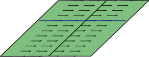
Figure 12.0.1: The vector field near a corner where both adjacent vertices are invariant.

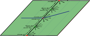
Figure 12.0.2: The vector field near a non-invariant corner where the broken trajectory (followed backwards) arrives at a red point. In this case, the continuation of the broken trajectory is determined by the dynamics of the vector field.

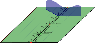
Figure 12.0.3: The vector field near a non-invariant corner where the broken trajectory (followed backwards) arrives at a green point. In this case, the continuation of the broken trajectory is determined by the center-stable manifold of the saddle point where the broken trajectory started.

12.1 Broken trajectories

In this subsection we construct two broken trajectories (recall Definition 11.1.5) associated to each saddle point of $\xi^{\mathrm{ro}}_{\mathrm{pol}}$ and define a topological path, the total broken trajectory as the union of their closures.

Let $\beta^{+}_{q}[0]$ be one of the two trajectories contained in the stable manifold of $\xi^{\mathrm{ro}}_{i,\theta}$ at a saddle point $q[0]=q\in D^{\mathrm{ro},\circ}_{i,\theta}$. We observe that since $\beta^{+}_{q}[0]$ is a trajectory of $\xi^{\mathrm{ro}}_{i,\theta}$, Lemma 12.0.1 says that its closure consists of $q[0]$ and another point $q[1]\neq q[0]$. Furthermore, since the center-stable manifold $S^{\mathrm{ro}}(q)$ meets transversely $D^{\mathrm{ro},\circ}_{i,\theta}$ at $q$ and it is an invariant (by $\hat{\xi}^{\mathrm{ro}}_{i}$) manifold we also have

$$\beta^{+}_{q}[0]\subset\overline{S^{\mathrm{ro}}(q)}\cap Y^{\mathrm{ro}}_{\theta}.$$

Assume that we have constructed a topological path $\beta^{+}_{q}[\ell]$ endowed with a filtration

$$\beta^{+}_{q}[0]\subseteq\beta^{+}_{q}[1]\subset\cdots\beta^{+}_{q}[\ell]$$

such that for each $k=0,\ldots,\ell$

1. the set $\mathrm{int}\left(\beta^{+}_{q}[k]\,\setminus\,\beta^{+}_{q}[k-1]\right)$ is an integral line of $\xi^{\mathrm{ro}}_{j,\theta}$ for some $j\in\mathcal{V}_{\mathrm{pol}}$.

2. the boundary of the closure $\overline{\beta^{+}_{q}[k]\setminus\beta^{+}_{q}[k-1]}$ consists of two points $q[k]$ and $q[k+1]$ which, by Lemma 12.0.1 satisfy that $q[k]\neq q[k+1]$.

3. $\beta^{+}_{q}[k]\subset\overline{S^{\mathrm{ro}}(q)}\cap\partial Y^{\mathrm{ro}}_{\theta}.$

The next is an exhaustive list, depending on where the point $q[\ell+1]$ lies, that indicates if the construction of the broken trajectory finishes or one has to construct $\beta^{+}_{q}[\ell+1]$ and iterate. At each step in which the algorithm is not finished, we verify that items (a), (b) and (c) above are satisfied.

1. The point $q[\ell+1]\in D^{\mathrm{ro},\circ}_{j,\theta}$ is a saddle point of $\xi^{\mathrm{ro}}_{j,\theta}$ for some $j\in\mathcal{V}$. Define

   $$\beta^{+}_{q}=\beta^{+}_{q}[\ell]\cup\{q[\ell+1]\}$$

   and finish the construction here.

2. The point $q[\ell+1]\in D^{\mathrm{ro},\circ}_{0,\theta}$ and it is a fountain of $\xi^{\mathrm{ro}}_{0,\theta}$. Define

   $$\beta^{+}_{q}=\beta^{+}_{q}[\ell]\cup\{q[\ell+1]\}$$

   and finish the construction here.

3. The point $q[\ell+1]\in D^{\mathrm{ro}}_{j,k}$ and both $j$ and $k$ are invariant vertices (as in figure Fig. 12.0.1). In this case there is a unique trajectory $\gamma[\ell+1]$ of $\xi^{\mathrm{ro}}_{k,\theta}$ that has $q[\ell+1]$ in its closure. We define

   $$\beta^{+}_{q}[\ell+1]=\beta^{+}_{q}[\ell]\cup q[\ell+1]\cup\gamma.$$

   Now we check that in this case the induction hypothesis items (a), (b) and (c) above are still satisfied. Indeed:

   1. $\mathrm{int}\left(\beta^{+}_{q}[\ell+1]\,\setminus\,\beta^{+}_{q}[\ell]\right)=\gamma[\ell+1]$ which is, by definition, an integral line.

   2. By Lemma 12.0.1, we have that the boundary of $\overline{\gamma[\ell+1]}$ consists exactly of two different points.

   3. By the last statement of 8.1.7, the closure of the center stable manifold $\overline{S^{\mathrm{ro}}(q)}$ meets $\partial Uro$ precisely at $\left(\{q[\ell+1]\}\cup\gamma[\ell]\cup\gamma[\ell+1]\right)\cap\partial U^{\mathrm{ro}}$. Here we are using that $S^{\mathrm{ro}}(q)$ is an invariant manifold contained in $Y^{\mathrm{ro}}_{\theta}$ that has $\gamma[\ell]$ in its closure.

4. The point $q[\ell+1]\in D^{\mathrm{ro}}_{j,k}$ and, at least one of the two vertices $j$ or $k$ is a non-invariant vertex. In this case, one of the following happens,

   1. we have $k\to j$ as in Fig. 12.0.2. This case is similar to the previous one: there is a unique trajectory $\gamma[\ell+1]$ of $\xi^{\mathrm{ro}}_{k,\theta}$ that has $q[\ell+1]$ in its closure. We define

      $$\beta^{+}_{q}[\ell+1]=\beta^{+}_{q}[\ell]\cup q[\ell+1]\cup\gamma[\ell+1].$$

      Again, the items (a) and (b) are verified directly. And item (c) follows because by Lemma 8.2.6, ii the Hessian of $\xi^{\mathrm{ro}}_{U}$ is elementary along the normal bundle and, since $S^{\mathrm{ro}}(q)$ is an invariant manifold contained in $Y^{\mathrm{ro}}_{\theta}$ that has $\gamma[\ell]\cup\{q[\ell]\}$ in its closure, then $S^{\mathrm{ro}}(q)$ must also have the only trajectory of $\xi^{\mathrm{ro}}_{k,\theta}$ that has $q[\ell]$ in its closure.

   2. We have $j\to k$ as in Fig. 12.0.3. In this case there is not a unique trajectory of $\xi^{\mathrm{ro}}_{k,\theta}$ that has $q[\ell+1]$ in its closure. However, we can apply the same reasoning as in the previous case and use that $S^{\mathrm{ro}}(q)$ is an invariant manifold contained in $Y^{\mathrm{ro}}_{\theta}$ that has $\gamma[\ell]\cup\{q[\ell]\}$ in its closure, then, by the non-degeneracy of the Hessian Lemma 8.2.6, ii, $S^{\mathrm{ro}}(q)$ can only have a unique trajectory of $\xi^{\mathrm{ro}}_{k,\theta}$ that has $q[\ell]$ in its closure $Y^{\mathrm{ro}}_{\theta}$. Then items (a) and (b) are item (c) verified.

Definition 12.1.1.

For each $q\in\Sigma^{\mathrm{ro}}_{i,\theta}$ that is a saddle point of $\xi^{\mathrm{ro}}_{i,\theta}$ define the set

$$\beta_{q}=\beta^{+}_{q}\cup\beta^{-}_{q}\cup\{q\}$$

and call it the total broken trajectory of $\xi^{\mathrm{ro}}_{i,\theta}$ at $q$.

Lemma 12.1.2.

We have

$$\beta_{q}\subset\overline{(\pi^{\mathrm{ro}}_{\mathrm{pol}})^{-1}(S^{\mathrm{ro}}(q))}\cap\partial Y^{\mathrm{ro}}_{\theta}.$$

Proof.

It follows from the construction of the broken trajectory above and that the property item (c), which is satisfied at each step of the construction, says that that $\beta_{q}^{+}[k]\subset\overline{(\pi^{\mathrm{ro}}_{\mathrm{pol}})^{-1}(S^{\mathrm{ro}}(q))}\cap\partial Y^{\mathrm{ro}}_{\theta}$. ∎

Definition 12.1.3.

We define the spine at radius $0$ and angle $\theta$, and denote it by $S^{\mathrm{ro}}_{\theta}$, as the union of all the total broken trajectories associated with all the saddle points of the vector fields $\xi^{\mathrm{ro}}_{i,\theta}$ for all $i\in\mathcal{V}$. That is,

$$S^{\mathrm{ro}}_{\theta}=\bigcup_{\begin{subarray}{c}i\in\mathcal{V}\\ q\text{ is a saddle point of }\xi^{\mathrm{ro}}_{i,\theta}\end{subarray}}\beta_{q}$$

As we will see later in Example 12.2.18, the spine at radius $0$ and angle $\theta$ is not in general a spine. In a sequel to this work we will workout some further genericity conditions under which for a generic analytical type representing a particular topological type and for a generic angle, the spine at radius $0$ and angle $\theta$ is a spine. In Section 12 we construct a quotient of the spine at radius $0$ which is always a spine for a quotient of the Milnor fiber at radius $0$ which is homeomorphic to the Milnor fiber.

12.2 The Petri dishes

In this section we analyze the vector field and the broken trajectories inside the connected components of the part of the Milnor fiber that corresponds to the non-invariant graph. We use Notation 11.1.8.

Lemma 12.2.1.

Let $\Xi$ be a branch (recall Definition 3.4.3) of $\Gamma_{\mathrm{pol}}$ at a vertex $i$ of $\Gamma_{\mathrm{pol}}\setminus\Upsilon$. Then $F^{\mathrm{ro}}_{\theta}[\Xi]$ is a disjoint union of disks. Moreover, if $ij$ is the edge that joins $\Xi$ with $\Gamma_{\mathrm{pol}}\setminus\Xi$, then $F^{\mathrm{ro}}_{\theta}[\Xi]$ is a disjoint union of $\gcd(m_{i},m_{j})$ disks.

Proof.

That $F^{\mathrm{ro}}_{\theta}[\Xi]$ is a disjoint union of disks follows from Lemma 6.4.2 that implies, that in $\Gamma_{\mathrm{min}}$, the graph $\Xi$ is a bamboo. The process of blowing up more to get to $\Gamma_{\mathrm{pol}}$ may introduce new vertices, but does not change the topology of the Milnor fiber. The statement on the number of connected components follows because near the intersection point of $\Xi$ with the rest of $\Gamma_{\mathrm{pol}}$, the Milnor fiber at radius $0$ looks like the Milnor fiber of $u^{m_{i}}v^{m_{j}}$ which is a disjoint union of $\gcd(m_{i},m_{j})$ cylinders. ∎

Definition 12.2.2.

Let $\Xi$ be a branch of $\Gamma_{\mathrm{pol}}$ at a vertex $i$ of $\Gamma_{\mathrm{pol}}\setminus\Upsilon$. We call each of the disks in $F^{\mathrm{ro}}_{\theta}[\Xi]$, a Petri dish. We denote Petri dishes by ${\mathbb{D}}_{\theta}$.

We say that a Petri dish is maximal if it is not strictly contained in any other Petri dish.

Next we introduce some useful notation for this subsection.

Notation 12.2.3.

Let ${\mathbb{D}}_{\theta}$ be a Petri dish coming from some branch $\Xi$ as in Definition 12.2.2.

We denote by $\beta[{\mathbb{D}}_{\theta}]$ the union of all the broken trajectories that start at some $D^{\mathrm{ro}}_{i,\theta}$ with $i\in\mathcal{V}_{\Xi}$, intersected with ${\mathbb{D}}_{\theta}$. That is,

$$\beta[{\mathbb{D}}_{\theta}]=\left(\bigcup_{\begin{subarray}{c}q\in\Sigma_{i,\theta}\\ i\in\mathcal{V}_{\Xi}\end{subarray}}\beta_{q}\right)\cap{\mathbb{D}}_{\theta}.$$

We denote by $S[{\mathbb{D}}_{\theta}]$ the part of the spine at radius $0$ that lies in ${\mathbb{D}}_{\theta}$. That is

$$S[{\mathbb{D}}_{\theta}]=S^{\mathrm{ro}}_{\theta}\cap{\mathbb{D}}_{\theta}.$$

A Petri dish ${\mathbb{D}}_{\theta}$ inherits a the structure of a stratified topological manifold with smooth strata. But it does not have, a priori, a smooth structure. In the the rest of this section we make use of Poincaré-Hopf Index theorem to prove results about the set $\beta[{\mathbb{D}}_{\theta}]$ and, in order to formalize such arguments we need to put a smooth structure on ${\mathbb{D}}_{\theta}$.

Lemma 12.2.4.

Let ${\mathbb{D}}_{\theta}$ be a Petri dish associated with a branch $\Xi$ with vertex set $\mathcal{V}_{\Xi}$. Then, ${\mathbb{D}}_{\theta}$ admits a smooth structure and the restricted vector field $\xi^{\mathrm{ro}}_{{\mathbb{D}}_{\theta}}=\xi^{\mathrm{ro}}_{\mathrm{pol}}|_{D_{\theta}}$ is a continuous vector field on ${\mathbb{D}}_{\theta}$.

Proof.

Each connected component ${\mathbb{D}}_{i,\theta}$ of $D^{\mathrm{ro}}_{i,\theta}$ can be thought of as a cobordism between the connected components $\partial_{j}{\mathbb{D}}_{i,\theta}$ of $\partial{\mathbb{D}}_{i,\theta}$ corresponding to edges $j\to i$ and the connected components $\partial_{k}{\mathbb{D}}_{i,\theta}$ of $\partial{\mathbb{D}}_{i,\theta}$ corresponding to edges $i\to k$.

Furthermore, let $ij$ be an edge $j\to i$. Then, there is a diffeomorphism

$$\iota_{ij}:\partial_{j}{\mathbb{D}}_{i,\theta}\to\partial_{i}{\mathbb{D}}_{j,\theta}$$

induced by the structure of fiber product (recall Remark 4.2.3) that identifies both sets of boundary components. Then, by [Mil65, Theorem 1.4], there exists a smooth structure on ${\mathbb{D}}_{i,\theta}\sqcup_{\iota_{ij}}{\mathbb{D}}_{j,\theta}$ which is compatible with each of the smooth structures on ${\mathbb{D}}_{i,\theta}$ and ${\mathbb{D}}_{j,\theta}$.

By definition, the vector field $\xi^{\mathrm{ro}}_{{\mathbb{D}}_{\theta}}$ is well defined on (and tangent to) $D^{\mathrm{ro}}_{i,j,\theta}$.

By iteratively applying this reasoning, we get a smooth structure on all ${\mathbb{D}}_{\theta}$ and a continuous vector field on it. Furthermore, this vector field coincides with $\xi^{\mathrm{ro}}_{i,\theta}$, up to multiplication by a real positive function, on each of the pieces of ${\mathbb{D}}_{\theta}$.

∎

Remark 12.2.5.

Note that the vector field $\xi^{\mathrm{ro}}_{{\mathbb{D}}_{\theta}}$ is a continuous (by construction) vector field but, in general, it is not $C^{1}$.

Definition 12.2.6.

We denote by $\xi^{\mathrm{ro}}_{{\mathbb{D}}_{\theta}}$ the continuous vector field defined on ${\mathbb{D}}_{\theta}$ with the smooth structure.

Remark 12.2.7.

1. By definition, $\beta[{\mathbb{D}}_{\theta}]\subseteq S[{\mathbb{D}}_{\theta}]$. And, in general, the above is not an equality as we will see later in an example.

2. The vector field $\xi^{\mathrm{ro}}_{{\mathbb{D}}_{\theta}}$ does not have any non-zero index singularities in the interior of ${\mathbb{D}}_{\theta}\setminus\beta[{\mathbb{D}}_{\theta}]$. This is because $\beta[{\mathbb{D}}_{\theta}]$ contains all the saddle points by construction and the other singularities are by Lemma 8.2.6 half-fountain-half-saddle or half-sink-half saddle points, (i.e. they are green and red points like those of fig. 8.2.1) which all have index $0$.

3. By definition of broken trajectory, the set $\beta[{\mathbb{D}}_{\theta}]$ seen as graph, if it has vertices of valency $1$, it has they have to lie on $\partial{\mathbb{D}}_{\theta}$.

12.2.8.

Here we deduce an easy relative version of the Poincaré-Hopf index theorem for vector fields on surfaces with boundary. Let $F$ be an oriented compact surface of genus $g$ with $b>0$ boundary components, and let $\xi_{F}$ be a vector field on $F$ which is also tangent to $\partial F$. Assume furthermore that $\xi$ has isolated singularities (some of them might be on the boundary). Now take the double-surface $2F$ of $F$: that is, consider $-F$ (which is the surface with opposite orientation) and glue $-F$ to $F$ along their boundaries by the identity map (note that the identity map inverts the orientation from $\partial F$ to $\partial(-F)$). The surface $-F$ comes naturally equipped with a vector field $\xi_{-F}$ which is identified with $\xi_{F}$ on $\partial(-F)$ by the identity map. Thus, we have a well defined vector field $\xi_{2F}$ defined on $2F$ with a isolated singularities. Observe that the surface $2F$ is a closed oriented surface of genus $2g+b-1$. This construction allows us to do two things:

1. Assign an index to isolated singularities on the boundary: for an isolated singularity $p\in\partial F$ of $\xi_{F}$, we define the index of $\xi_{f}$ at $p$ by the formula

   (12.2.9) $${\mathrm{Ind}}_{\xi_{F}}(p)=\frac{1}{2}{\mathrm{Ind}}_{\xi_{2F}}(p)$$

   where, on the right-hand side, $p$ is seen as a point in $2F$.

2. We compute a relative version of the Poincaré-Hopf index theorem. By applying the classical theorem to the surface $2F$, we get:

   $$2\sum_{p\in\mathring{F}}{\mathrm{Ind}}_{\xi_{F}}(p)+\sum_{p\in\partial F\subset F}{\mathrm{Ind}}_{\xi_{2F}}(p)=2-2(2g+b-1).$$

   which, after dividing by $2$ and applying the previous definition eq. 12.2.9 yields,

   (12.2.10) $$\sum_{p\in F}{\mathrm{Ind}}_{\xi_{F}}(p)=2-2g-b=\chi(F).$$

   Where the term on the left-hand side allows for $\xi_{F}$ to have isolated singularities on the boundary of $F$.

Next we classify all the singularities that might appear on the boundary of connected components of ${\mathbb{D}}_{\theta}\setminus\beta[{\mathbb{D}}_{\theta}]$.

Lemma 12.2.11.

Let $\Delta$ be the closure of a connected component of ${\mathbb{D}}_{\theta}\setminus\beta[{\mathbb{D}}_{\theta}]$ and assume that $\partial\Delta$ is an embedded circle. Then the vector field $\left.\xi^{\mathrm{ro}}_{{\mathbb{D}}_{\theta}}\right|_{\Delta}$ has no non-zero index singularities on the interior of $\Delta$ and, on $\partial\Delta$ it may have

1. Quarter-fountain-quarter-saddle, quarter-sink-quarter-saddle, quarter saddle points as the only singularities of index $0$ (see fig. 12.2.1),

2. half-sink, half-fountain points as the only singularities of index $1/2$ (see fig. 12.2.2),

3. half-saddle points as the only singularities of index $-1/2$ (see the right-hand side of fig. 12.2.3).

Proof.

The first part of the statement on the singularities in the interior of $\Delta$ is exactly Remark 12.2.7 item (ii). Now we notice that the only singularities that $\Delta$ might have, happen when $\partial\Delta$ crosses a singularity of $\left.\xi^{\mathrm{ro}}_{{\mathbb{D}}_{\theta}}\right|_{\Delta}$. So let $p\in\partial\Delta$ be a singularity of $\left.\xi^{\mathrm{ro}}_{{\mathbb{D}}_{\theta}}\right|_{\Delta}$, next we go through all the possible cases depending on where $p$ lies.

Case 1. If $p\in\partial{\mathbb{D}}_{\theta}$, then $p$ is either a half-fountain or a half-sink point when seen as a singularity of $\xi^{\mathrm{ro}}_{{\mathbb{D}}_{\theta}}$ (because of Lemma 8.2.6). In this case, $p$ seen as a singularity of $\left.\xi^{\mathrm{ro}}_{{\mathbb{D}}_{\theta}}\right|_{\Delta}$ can only be a half-fountain (red vertex) or a half-sink (green vertex) singularity. This covers item (ii).

Case 2. If $p$ is in the interior of ${\mathbb{D}}_{\theta}$, then there are two possibilities:

1. $p$ is a saddle point of $\xi^{\mathrm{ro}}_{{\mathbb{D}}_{\theta}}$. In this case the segment of $\partial\Delta$ that passes through $p$ might be formed either by a stable trajectory and an unstable trajectory (the blue singularity of fig. 12.2.1) giving a singularity of index $0$, or by two stable trajectories (the right-hand side of fig. 12.2.3) giving a singularity of index $-1/2$. Note that it can’t happen that this segment is formed by two unstable trajectories (left-hand side of fig. 12.2.3) since $\beta[{\mathbb{D}}_{\theta}]$ contains by definition the stable trajectories of all saddle points.

2. $p$ is a red or green point of a smaller Petri dish ${\mathbb{D}}^{\prime}_{\theta}\subset{\mathbb{D}}_{\theta}$. In this case the segment of $\partial\Delta$ that passes through $p$ must correspond to a broken trajectory that either enters the smaller Petri dish ${\mathbb{D}}^{\prime}_{\theta}$ or exits ${\mathbb{D}}^{\prime}_{\theta}$ (this corresponds to the two left figures of fig. 12.2.1). Note that by the construction of broken trajectories, no broken trajectory can contain a segment of the boundary of a Petri dish since boundaries of Petri dishes do not have saddle points of $\xi^{\mathrm{ro}}_{{\mathbb{D}}_{\theta}}$.

These two subcases cover all the possibilities in item (i) and item (iii) finishing the proof. ∎

Figure 12.2.1: Singularities (red, green and blue points) of index $0$ of a vector field tangent to the boundary (grey thick line) of a surface.

Figure 12.2.2: Singularities (green and red points) of index $1/2$ of a vector field tangent to the boundary (grey thick line) of a surface.

Figure 12.2.3: Singularities (blue points) of index $-1/2$ of a vector field tangent to the boundary (grey thick line) of a surface.

Lemma 12.2.12.

Let ${\mathbb{D}}_{\theta}$ be a Petri dish coming from some graph $\Xi$. Let $i$ be the root of $\Xi$ and let $j$ be the vertex in $\Gamma_{\mathrm{pol}}\setminus\Xi$ to which it is connected. Then the number of saddle points $I$ of $\xi^{\mathrm{ro}}_{{\mathbb{D}}_{\theta}}$ is equal to:

(12.2.13) $$I=-\frac{\left|\begin{matrix}\varpi_{i}&m_{i}\\ \varpi_{j}&m_{j}\end{matrix}\right|}{\gcd(m_{i},m_{j})}-1.$$

In particular, $\beta[{\mathbb{D}}_{\theta}]$ is non-empty if and only if $I\geq 1$, equivalently, if there are at least $2$ red points on $\partial{\mathbb{D}}_{\theta}$.

Proof.

The term with the fraction on eq. 12.2.13 the number of red points (and green points) on $\partial{\mathbb{D}}_{\theta}$ (Lemma 8.4.1). These singularities look on ${\mathbb{D}}_{\theta}$ like half sinks (green points) and half fountains (red points). See fig. 12.2.2. These have relative Poincaré-Hopf index equal to $1/2$. By Remark 12.2.7 item (ii) the only singularities of non-zero index on the interior of ${\mathbb{D}}_{\theta}$ are saddle points. A direct application of eq. 12.2.10 yields the result since:

$$-\frac{\left|\begin{matrix}\varpi_{i}&m_{i}\\ \varpi_{j}&m_{j}\end{matrix}\right|}{\gcd(m_{i},m_{j})}-I=1.$$

That $\beta[{\mathbb{D}}_{\theta}]$ is non-empty if and only if there is at least $1$ saddle point in ${\mathbb{D}}_{\theta}$ follows from the definition of the broken trajectories which start at all saddle points. ∎

Corollary 12.2.14.

The set $\beta[{\mathbb{D}}_{\theta}]$ does not contain any green points in $\partial{\mathbb{D}}_{\theta}$.

Proof.

A green point is, by definition, half a sink. In order for $\beta[{\mathbb{D}}_{\theta}]$ to contain a green point it must have happened that a broken trajectory starting at $q\in{\mathbb{D}}_{\theta}$ must have exited ${\mathbb{D}}_{\theta}$ and re-enter it through that green point. But Lemma 11.1.9 prevents this. ∎

Lemma 12.2.15.

Each connected component of $\beta[{\mathbb{D}}_{\theta}]$:

1. is connected to some red vertex on $\partial{\mathbb{D}}_{\theta}$ and

2. is contractible.

Proof.

Let $q\in\beta[{\mathbb{D}}_{\theta}]$ be a saddle point of some $\xi^{\mathrm{ro}}_{i,\theta}$ with $i\in\mathcal{V}_{\Xi}$.

Claim 1. The broken trajectory $\beta^{+}_{q}$ can’t end at $q$.

Proof of Claim 1..

If $\beta^{+}_{q}$ ends at $q$, because of Lemma 11.1.9, it must be contained entirely in ${\mathbb{D}}_{\theta}$. Now we apply a similar reasoning as in the proof of Lemma 11.1.9: contract each of the smaller Petri dishes contained in ${\mathbb{D}}_{\theta}$ to a point. We obtain a loop, formed by integral lines of a vector field that, by Lemma 9.3.3, admits a potential which is contradictory. ∎

By the previous claim, either the broken trajectory ends at another saddle point $q^{\prime}\in{\mathbb{D}}_{\theta}$ or it has to exit $\partial{\mathbb{D}}_{\theta}$ by some red point on $\partial{\mathbb{D}}_{\theta}$ (note that it can only exit ${\mathbb{D}}_{\theta}$ through a red point since broken trajectories are constructed following the flow backwards). If it exits ${\mathbb{D}}_{\theta}$ through a red point, we are done proving item (i).

Assume otherwise it arrives at another saddle point $q^{\prime}$. now consider one of the broken trajectories $\beta^{\prime+}_{q^{\prime}}$ associated with $q^{\prime}$.

Claim 2. The broken trajectory $\beta^{\prime+}_{q^{\prime}}$ can’t end at $q$.

Proof of Claim 2..

The proof is very similar to the previous claim: contract each of the smaller Petri dishes contained in ${\mathbb{D}}_{\theta}$ to a point. We obtain a loop, formed by integral lines of a vector field that, by Lemma 9.3.3, admits a potential which is contradictory. ∎

After claim 2, we get that the broken trajectory $\beta^{\prime+}_{q^{\prime}}$ either ends at a red point in $\partial{\mathbb{D}}_{\theta}$ or it gets to another saddle point $q^{\prime\prime}$ that, following a similar reasoning to that of Claim 1 and 2, must be different from $q$ and $q^{\prime}$. Now we can iterate this process and get that, after each step, we either arrive at a red point in $\partial{\mathbb{D}}_{\theta}$ or to a saddle point that we have not visited before. But there are only finitely many saddle points contained in ${\mathbb{D}}_{\theta}$. This proves item (i).

Now we prove item (ii). The proof of item (i) already shows that there can be no loops of a connected component in the interior of ${\mathbb{D}}_{\theta}$. Assume that we have a loop $L$ that contains at least a point $p$ in $\partial{\mathbb{D}}_{\theta}$. This point is necessarily red by 12.2.14. Furthermore, assume that this loop does not contain any other loops of $\beta[{\mathbb{D}}_{\theta}]$ in the disk that it encloses, for if it does, we can always choose one of the smaller loops. Then $L$ is a concatenation of paths $L_{1},\ldots,L_{n}$ and red points $p_{1},\ldots,p_{n}$. The loop $L$ encloses a disk, which by Remark 12.2.7 item (ii) and by our hypothesis on the minimality of $L$, does not contain any non-zero index singularities. Since each $L_{k}$ joins two red points, it must contain at least one singularity of index $-1/2$: indeed, if for example $L_{1}$ joins $p_{1}$ with $p_{2}$, then there are two trajectories of $\xi^{\mathrm{ro}}_{{\mathbb{D}}_{\theta}}$ inside $L_{1}$ with opposite sign, so necessarily there is a saddle point on $L_{1}$. Thus, using eq. 12.2.10 we get

$$\sum_{i=1}^{n}\left({\mathrm{Ind}}_{\xi^{\mathrm{ro}}_{{\mathbb{D}}_{\theta}}}(p_{i})+\sum_{q\in L_{i}}{\mathrm{Ind}}_{\xi^{\mathrm{ro}}_{{\mathbb{D}}_{\theta}}}(q)\right)\leq\frac{n}{2}-\frac{n}{2}=0.$$

which contradicts the fact that the Euler characteristic of the disk enclosed by $L$ is equal to $1$. ∎

Corollary 12.2.16.

The closure of each connected component of ${\mathbb{D}}_{\theta}\setminus\beta[{\mathbb{D}}_{\theta}]$ is a closed disk.

Proof.

By Lemma 12.2.15, each connected component $\beta[{\mathbb{D}}_{\theta}]$ is connected to some red vertex and it is a tree. The interior of the complement of a tree contained in a disk is a disjoint union of open disks provided that the tree is connected to at least a point of the boundary of the disk. Now, by Remark 12.2.7 item (iii), each connected component of $\beta[{\mathbb{D}}_{\theta}]$ does not have vertices of valency $1$ in the interior of ${\mathbb{D}}_{\theta}$, so the boundary of the closure of each connected component must be an embedded circle. ∎

Proposition 12.2.17.

If the set $\beta[{\mathbb{D}}_{\theta}]$ is non-empty, then

1. it is connected,

2. it is contractible,

3. it contains all the red points in $\partial{\mathbb{D}}_{\theta}$.

Proof.

We construct a (possibly disconnected) abstract graph $\tilde{\beta}$:

1. The set of vertices is the union of the saddle points of $\xi^{\mathrm{ro}}_{{\mathbb{D}}_{\theta}}$ and the red vertices on $\partial{\mathbb{D}}_{\theta}$.

2. there is an edge between a saddle point and another saddle point or between a saddle point and a red point if there is a broken trajectory in $\beta[{\mathbb{D}}_{\theta}]$ that joins them.

The underlying $1$-dimensional $CW$-complex of $\tilde{\beta}$ is homeomorphic to $\beta[{\mathbb{D}}_{\theta}]$ union all the red vertices. And we have a natural injective map $\beta[{\mathbb{D}}_{\theta}]\hookrightarrow\tilde{\beta}$ that realizes $\beta[{\mathbb{D}}_{\theta}]$ in $\tilde{\beta}$. Since each red vertex can be thought of as a tree and the connected components of $\beta[{\mathbb{D}}_{\theta}]$ are trees by Lemma 12.2.15 item (ii), the Euler characteristic of $\tilde{\beta}$ counts the number of connected components. If we let $R$ be the number of red points, $I$ the number of saddle points and $e$ the number edges, we get that by construction of the broken trajectories, $e=2I$ and

$$\chi(\tilde{\beta})=R+I-e=R-I.$$

But $R-I=1$ by Lemma 12.2.12. So $\tilde{\beta}$ is connected an contains all the red points, we conclude items (i) and (iii).

That $\beta[{\mathbb{D}}_{\theta}]$ is contractible item (ii) follows directly from Lemma 12.2.15 item (ii). ∎

Example 12.2.18.

In this example we show that the union of broken trajectories starting at all saddle points does not, in general, form a spine for the Milnor fiber at radius $0$.

Consider the plane curve singularity $C$ defined by $f(x,y)=y^{6}-2y^{3}x^{4}-3x^{8}+yx^{7}$. The plane curve $C$ consists of two branches which are Brieskorn-Pham singularities of type $(3,4)$ with the same tangent. The polar curve $P$ is defined by the equation $f_{y}=6y^{5}-6y^{2}x^{4}+x^{7}$ and has two branches. The strict transform of one of the branches passes through the exceptional divisor $D_{2}$ and the other one through the divisor $D_{3}$. The divisor $D_{3}$ is an invariant divisor and so the point $\tilde{P}\cap D_{3}$ is a base point of the Jacobian ideal by Lemma 6.4.10 item (iii). After blowing up this base point once, we get the dual graph on the bottom of fig. 12.2.4.

Figure 12.2.4: On top the dual graph of the minimal resolution of $C$. On bottom, the resolution resulting from blowing up the base point of the divisor $D_{3}$ once. In blue we have the strict transform of the polar curve $P$ which has two branches.

Let’s look at the divisor $D_{3}$ in the minimal resolution of the plane curve. For that, we consider the monomial transformation

$$\pi(u,v)=(u^{3}v^{2},u^{4}v^{3})$$

which sees a neighborhood around $D_{3}\cap D_{2}$. Using $\tau_{3}=8$ and $\tau_{2}=5$ we can compute the restriction of the extension of the vector field over $D_{3}^{\circ}$ in this chart (see fig. 12.2.5 for its representation) and we get the expression:

$$\xi_{3}=-\frac{18{\left(\bar{v}-1\right)}}{|v|^{4}\left(\bar{v}^{2}-2\bar{v}-3\right)}.$$

The intersection with the two components of the strict transform of $C$ are on the real points $-1,3\in\mathbb{C}$. We see (fig. 12.2.5) that there is a trajectory of $\xi_{3}$ on $D_{3}^{\circ}$ that goes from the saddle point corresponding to the intersection point $D_{3}\cap D_{4}$. On $D_{2}$ there is another intersection point $\tilde{P}\cap D_{2}$.

Figure 12.2.5: The divisor $D_{3}$. The two black dots correspond with the intersection points of the strict transforms of the curve $C$. The blue dot corresponds with the intersection point of $D_{3}$ and $D_{4}$. The circled dot corresponds with the intersection point of $D_{2}$ and $D_{3}$. The blue segment is a trajectory.

Now we analyze what happens at the level of the Milnor fiber at radius $0$. The multiplicity $m_{2}$ of $\pi^{*}f$ at $D_{2}$ is $16$. The multiplicity $m_{1}$ is $8$. This says that $D^{\mathrm{ro}}_{1,\theta}$ consists of $8$ disks and $D^{\mathrm{ro}}_{2,\theta}$ consists of $8$ cylinders for each $\theta\in\mathbb{R}/2\pi\mathbb{Z}$. Thus, on each of these $8$ cylinders, the vector field $\xi^{\mathrm{ro}}_{2,\theta}$ has $2$ saddle points. Furthermore, a computation yields that $\varpi_{2}=1$ and we know that $\varpi_{3}=0$. Therefore, using Lemma 8.2.4 iii we get that the each component of $D^{\mathrm{ro}}_{2,3,\theta}$ has $3$ red points (and $3$ green points). We conclude that for a generic angle $\theta$, one of the three red points on each cylinder is chosen by two half broken trajectories starting at the two saddle points on each connected component of $D^{\mathrm{ro}}_{2,\theta}$. We have, in total $24$ red points and $8$ of these are chosen by two half broken trajectories on their corresponding cylinders.

We analyze now what happens in $D_{4}$. The multiplicity $m_{4}=m_{3}=24$, so $D^{\mathrm{ro}}_{4,\theta}$ consists of $24$ disks. Since $\varpi_{4}=2$, each of these disks has $2$ red points and $2$ green points ($48$ of each in total). Moreover, $D_{4}$ intersects $\tilde{P}$ and so each of the $24$ disks of $D^{\mathrm{ro}}_{4,\theta}$ has a saddle point of $\xi^{\mathrm{ro}}_{4,\theta}$ on its interior. Each of the two red points on each component of $\partial D^{\mathrm{ro}}_{4,\theta}$ gets chosen by one of the broken trajectories associated with the saddle point.

The fact that there is a trajectory going from $D_{4}\cap D_{3}$ to $D_{3}\cap D_{2}$ yields that there are $24$ trajectories in $D^{\mathrm{ro}}_{3,\theta}$ joining the $24$ red points of $D^{\mathrm{ro}}_{2,3,\theta}$ with $24$ of the $48$ green points lying on $D^{\mathrm{ro}}_{3,4,\theta}$.

Let $p_{1},p_{2}\in D^{\mathrm{ro}}_{2,\theta}$ be two saddle points of $\xi^{\mathrm{ro}}_{2,\theta}$ lying on the same connected component of $D^{\mathrm{ro}}_{2,\theta}$. We know that the Hessian of $\xi^{\mathrm{ro}}_{2,3\theta}$ at the red points is non degenerate, so the two broken trajectories that start at $p_{1}$ and $p_{2}$ and end at the same red poin and arrive (flowing backwards) at this red point, with different tangents. After passing through the red points, both broken trajectories choose the same trajectory on $D^{\mathrm{ro}}_{3,\theta}$ and this is one of the $24$ trajectories that lie above the trajectory on $D_{3}^{\circ}$ connecting $D_{2}\cap D_{3}$ with $D_{3}\cap D_{4}$. Here, the closures of $S^{\mathrm{ro}}(p_{1})$ and $S^{\mathrm{ro}}(p_{2})$ intersect transversally along the trajectory in $D^{\mathrm{ro},\circ}_{3,\theta}$.

Figure 12.2.6: On the right part of the picture we see a neighborhood of the $D^{\mathrm{ro}}_{2,3,\theta}$. On the right we also see, in blue, the center-stable manifolds $S^{\mathrm{ro}}(p_{1})$ and $S^{\mathrm{ro}}(p_{2})$. On the left part of the picture we see a neighborhood of $D^{\mathrm{ro}}_{3,4,\theta}$. We see how the two center-stable manifolds define different trajectories in $D^{\mathrm{ro}}_{4,\theta}$ even though they define the same in $D^{\mathrm{ro}}_{3,\theta}$.

If $q$ is the green point in $D^{\mathrm{ro}}_{3,4,\theta}$ chosen by the common segment of the two broken trajectories, then the germs of $\overline{S^{\mathrm{ro}}(p_{1})}$ and $\overline{S^{\mathrm{ro}}(p_{2})}$ at $q$ define different manifolds, which by the non-degeneracy of the vector field $\xi^{\mathrm{ro}}_{\mathrm{pol}}$ at $q$, define different trajectories in $D^{\mathrm{ro}}_{4,\theta}$, that is $\overline{S^{\mathrm{ro}}(p_{1})}\cap D^{\mathrm{ro},\circ}_{4,\theta}$ and $\overline{S^{\mathrm{ro}}(p_{2})}\cap D^{\mathrm{ro},\circ}_{4,\theta}$ are two distinct trajectories of $\xi^{\mathrm{ro}}_{4,\theta}$. In fig. 12.2.7 we see the three qualitatively different possibilities and we see how all of them form $CW$ complexes that enclose a disk and so we conclude that in general the spine at radius $0$ and angle $\theta$ (Definition 12.1.3) is not a spine.

Figure 12.2.7: The three possibilities for the broken trajectories coming from one Petri dish and entering the Petri dish (flowing backwards) corresponding to the component of the polar curve that intersects $D_{4}$.

Remark 12.2.19.

In the previous example, a special situation occurs, which can be seen in fig. 12.2.5. The blue point has two trajectories emerging from it, and one of the trajectories converges to the white point. In a generic situation, each trajectory emerging from the blue point would converge to one of the sinks. This picture cannot be made generic by perturbing the metric by 9.1.10. It can, however be made generic by an equisingular deformation of the analytic structure of $(C,0)$. Such deformations will be further studied in a subsequent manuscript.

12.3 The invariant Milnor fibration

In this subsection we introduce a $\mathcal{C}^{\infty}$-fibration which is equivalent to the Milnor fibration and whose total space is a quotient of the exceptional part of the boundary of $Y^{\mathrm{ro}}_{\mathrm{pol}}$.

12.3.1.

Let

$$\partial_{\mathcal{V}}Y^{\mathrm{ro}}_{\mathrm{pol}}=\bigcup_{i\in\mathcal{V}_{\mathrm{pol}}}D^{\mathrm{ro}}_{i}.$$

We consider the equivalence relation $\sim_{\Upsilon}$ that collapses each Petri dish ${\mathbb{D}}_{\theta}$ to a point. Thus, $\sim_{\Upsilon}$ is the finest equivalence relation of $\partial_{\mathcal{V}}Y^{\mathrm{ro}}_{\mathrm{pol}}$ for which $p\sim_{\Upsilon}p^{\prime}$ for all $p,p^{\prime}\in D^{\mathrm{ro}}_{i,\theta}$, for any $\theta$ and $i\in\mathcal{V}_{\mathrm{pol}}\setminus\mathcal{V}_{\Upsilon}$. Denote the quotient space by

$$D^{\mathrm{ro}}_{\Upsilon}=\partial_{\mathcal{V}}Y^{\mathrm{ro}}_{\mathrm{pol}}/\sim_{\Upsilon}$$

Thus, the image of the Milnor fiber at radius $0$ in this quotient space is homeomorphic to the Milnor fiber at radius $0$. Since $\arg^{\mathrm{ro}}$ takes constant value along Petri dishes, we have a well defined map

$$\arg_{\Upsilon}^{\mathrm{ro}}:D^{\mathrm{ro}}_{\Upsilon}\mapsto\mathbb{R}/2\pi\mathbb{Z}$$

on the quotient space.

12.3.2.

We construct a $\mathcal{C}^{\infty}$ structure on the space $D^{\mathrm{ro}}_{\Upsilon}$ as follows. First, we construct a $\mathcal{C}^{\infty}$ structure on $D^{\mathrm{ro}}_{i}/\sim_{\Upsilon}$, for $i\in\mathcal{V}_{\Upsilon}$. This space contains some number of copies of embedded $S^{1}$, which are the collapsed Petri dishes. More precisely, if $ik$ is an edge corresponding to an invariant vertex $i$ and a non-invariant vertex $k$, take a coordinate $v$ in a neighborhood $V\subset D_{i}$ of $D_{i}\cap D_{k}$. Then $\sigma^{*}v$ takes constant value along $D^{\mathrm{ro}}_{i,k}$. This induces a function $v^{\mathrm{ro}}:\sigma^{-1}(V)\to\mathbb{C}$, which, along with $\arg^{\mathrm{ro}}(f)$ endows $\sigma^{-1}(V)$ with a smooth structure. This way, $D^{\mathrm{ro}}_{i}/\sim_{\Upsilon}$ is a compact $3$ dimensional manifold whith boundary components which are tori, corresponding to invariant edges.

The space $D^{\mathrm{ro}}_{\Upsilon}$ is obtained by gluing together the pieces $D^{\mathrm{ro}}_{i}/\sim_{\Upsilon}$ along the boundary tori (via the identity map). Let $ij$ be an invariant edge with $j\to i$. We obtain coordinates near the embedded torus $D^{\mathrm{ro}}_{ij}$ as follows. Take Grobman-Hartman coordinates $u,v$ in a chart $U$ around the intersection point $D_{i}\cap D_{j}$ as given by Lemma 8.1.1 such that $\{u=0\}=D_{i}\cap U$ and $\{v=0\}=D_{j}\cap U$. In particular, as in eq. 8.1.8, the vector field $\xi_{U}$ is given as

$$\xi_{U}=d\left(\begin{matrix}c_{0,j}u\\ -c_{0,i}v\\ \end{matrix}\right)$$

where $d>0$. This way, we get polar coordinates $u=re^{i\alpha}$ and $v=se^{i\beta}$ in $U^{\mathrm{ro}}=\sigma^{-1}(U)$. The functions $\alpha,\beta:U^{\mathrm{ro}}\to S^{1}$ restrict to functions in a neighborhood of $D^{\mathrm{ro}}_{ij}=D^{\mathrm{ro}}_{i}\cap D^{\mathrm{ro}}_{j}$, giving two coordinates in $D^{\mathrm{ro}}_{\Upsilon}\cap U^{\mathrm{ro}}$. A third coordinate $t$ is constructed by setting

$$t:D^{\mathrm{ro}}_{\Upsilon}\to\mathbb{R},\qquad t(q)=\begin{cases}s(q)&q\in D^{\mathrm{ro}}_{i},\\ -r(q)&q\in D^{\mathrm{ro}}_{j}.\\ \end{cases}$$

Lemma 12.3.3.

The map $\arg_{\Upsilon}^{\mathrm{ro}}(f):D^{\mathrm{ro}}_{\Upsilon}\mapsto\mathbb{R}/2\pi\mathbb{Z}$, induced by $\arg^{\mathrm{ro}}(f)$ is a $\mathcal{C}^{\infty}$ locally trivial fibration with fiber $F^{\mathrm{ro}}_{\Upsilon,\theta}$, which is equivalent to the Milnor fibration.

Proof.

The space $D^{\mathrm{ro}}_{\Upsilon}$ is compact, and the function $\arg^{\mathrm{ro}}_{\Upsilon}(f)$, and its restriction to the boundary of $D^{\mathrm{ro}}_{\Upsilon}$, is a submersion. Therefore, the lemma follows from Ehresmann’s fibration theorem.

Indeed, take any $q\in D^{\mathrm{ro}}_{\Upsilon}$. If $q\in D^{\mathrm{ro},\circ}_{i}$ for some $i\in\mathcal{V}_{\Upsilon}$, then it is clear that $\arg^{\mathrm{ro}}_{\Upsilon}(f)$ is a submersion at $q$. If $q$ is the image of some Petri dish, then $\arg^{\mathrm{ro}}_{\Upsilon}(f)$ is a coordinate near $q$, in particular, it is a submersion at $q$. If $q\in D^{\mathrm{ro}}_{ij}$, where $ij$ is an invariant edge, then $\arg^{\mathrm{ro}}_{\Upsilon}(f)|_{D^{\mathrm{ro}}_{ij}}$ is already a submersion, as seen in Lemma 4.2.4, and the same argument applies to the boundary components of $D^{\mathrm{ro}}_{\Upsilon}$. ∎

Definition 12.3.4.

We call

$$\arg_{\Upsilon}^{\mathrm{ro}}(f):D^{\mathrm{ro}}_{\Upsilon}\mapsto\mathbb{R}/2\pi\mathbb{Z}$$

the invariant Milnor fibration. For each $\theta\in\mathbb{R}/2\pi\mathbb{Z}$ we denote by

$$F^{\mathrm{ro}}_{\Upsilon,\theta}=(\arg_{\Upsilon}^{\mathrm{ro}})(f)^{-1}(\theta)$$

the corresponding fiber and call it the invariant Milnor fiber.

12.3.5.

Next, we construct a vectorfield defined on $D^{\mathrm{ro}}_{\Upsilon}$. In $D^{\mathrm{ro},\circ}_{i}$, outside a small neighbourhood of the boundary tori $D^{\mathrm{ro}}_{ij}$, the vector field coincides with $\xi^{\mathrm{ro}}_{i}$. Let $ij$ be an invariant edge, directed as $j\to i$. Then, with a coordinate neighborhood $U$ with coordinates $u,v$ as in the above construction, define a vector field

$$\xi^{\mathrm{ro}}_{U,\Upsilon}=(1,0,0)$$

in the coordiantes $(t,\alpha,\beta)$. Note that this vector field is parallel to $\xi^{\mathrm{ro}}_{i}$ and $\xi^{\mathrm{ro}}_{j}$ outside $D^{\mathrm{ro}}_{ij}$. Using partition of unity, these vector fields add up to a global vector field on all of $D^{\mathrm{ro}}_{\Upsilon}$. This vector field is tangent to the Milnor fibers $F^{\mathrm{ro}}_{\Upsilon,\theta}$ for $\theta\in\mathbb{R}/2\pi\mathbb{Z}$.

Definition 12.3.6.

Denote by $\xi^{\mathrm{ro}}_{\Upsilon}$ the vector field on $D^{\mathrm{ro}}_{\Upsilon}$ constructed in the previous paragraph, and by $\xi^{\mathrm{ro}}_{\Upsilon,\theta}$ its restriction to the invariant Milnor fiber $F^{\mathrm{ro}}_{\Upsilon,\theta}$, for $\theta\in\mathbb{R}/2\pi\mathbb{Z}$.

Remark 12.3.7.

By construction, the trajectories of $\xi^{\mathrm{ro}}_{\Upsilon}$ pass transversally through the tori $D^{\mathrm{ro}}_{ij}$. In fact, as a set, a trajectory of $\xi^{\mathrm{ro}}_{\Upsilon}$ is a broken trajectory of $\xi^{\mathrm{ro}}$ in the invariant part of $\partial Y^{\mathrm{ro}}_{\mathrm{pol}}$.

Lemma 12.3.8.

There exists a real function $\phi^{\mathrm{ro}}_{\Upsilon}:D^{\mathrm{ro}}_{\Upsilon}\to\mathbb{R}$ such that $\xi^{\mathrm{ro}}_{\Upsilon}$ is gradient-like for it. That is,

$$d\phi^{\mathrm{ro}}_{\Upsilon}(\xi^{\mathrm{ro}}_{\Upsilon})>0$$

outside the singular points of $\xi^{\mathrm{ro}}_{\Upsilon}$. Setting $\phi^{\mathrm{ro}}_{\Upsilon,\theta}=\phi^{\mathrm{ro}}_{\Upsilon}|_{F^{\mathrm{ro}}_{\Upsilon,\theta}}$, we also have

$$d\phi^{\mathrm{ro}}_{\Upsilon,\theta}(\xi^{\mathrm{ro}}_{\Upsilon,\theta})>0$$

outside the singular points of $\xi^{\mathrm{ro}}_{\Upsilon,\theta}$.

Proof.

For any $i\in\mathcal{V}_{\Upsilon}$, the vector field $\xi_{i}$ has a potential $\phi_{i}$, given in Definitions 7.4.3 and 9.2.2. We set $\phi^{\mathrm{ro}}_{i}=\sigma^{*}\phi_{i}$. If $i$ has distance $k$ to $0$ in $\Upsilon$, rescale $\phi^{\mathrm{ro}}_{i}$ to take values in $[k,k+1]$. These functions glue together to the desired global function $\phi^{\mathrm{ro}}_{\Upsilon,\theta}$. ∎

Remark 12.3.9.

Let $ij$ be and edge of $\Gamma_{\mathrm{pol}}$ with $j$ invariant and $i$ non invariant (necessarily $j\to i$). Then, by Lemma 8.2.6 (see also fig. 8.2.1), the vector field $\xi^{\mathrm{ro}}_{\Upsilon,\theta}$ (by Lemma 8.4.1 item (iii)) has $\varpi_{i}m_{j}/\gcd(m_{j},m_{i})$-pronged singularities near the intersection points of $D^{\mathrm{ro}}_{j,\theta}$ with $\sigma_{\Upsilon}^{-1}(D_{i})$. See fig. 12.3.1.

12.3.10.

We extend the equivalence relation $\sim_{\Upsilon}$ trivially over $Y^{\mathrm{ro}}_{\mathrm{pol}}$, so that equivalence classes outside $\partial_{\mathcal{V}}Y^{\mathrm{ro}}_{\mathrm{pol}}\subset Y^{\mathrm{ro}}_{\mathrm{pol}}$ contain only one point. This way, the invariant Milnor fibration sits inside the space $Y^{\mathrm{ro}}_{\mathrm{pol}}/\sim_{\Upsilon}$, which projects by $\pi^{\mathrm{ro}}_{\mathrm{pol}}$ to $\mathbb{C}^{2}$ isomorphically outside $C$.

Definition 12.3.11.

Denote by

$$p_{\Upsilon}:Y^{\mathrm{ro}}_{\mathrm{pol}}\to Y^{\mathrm{ro}}_{\mathrm{pol}}/\sim_{\Upsilon}$$

the natural projection. Let $S^{\mathrm{ro}}_{\Upsilon,\theta}$ be the intersection of $F^{\mathrm{ro}}_{\Upsilon,\theta}$ with the closure of the strict transform of the total spine, that is,

$$S^{\mathrm{ro}}_{\Upsilon,\theta}=F^{\mathrm{ro}}_{\Upsilon,\theta}\cap\overline{p_{\Upsilon}\left((\pi^{\mathrm{ro}}_{\mathrm{pol}})^{-1}(S\setminus\{0\})\right)}.$$

We call $S^{\mathrm{ro}}_{\Upsilon,\theta}$ the invariant spine. Define also the total invariant spine as

$$S^{\mathrm{ro}}_{\Upsilon}=\bigcup_{\theta\in\mathbb{R}/2\pi\mathbb{Z}}S^{\mathrm{ro}}_{\Upsilon,\theta}.$$

Theorem 12.3.12.

The invariant spine $S^{\mathrm{ro}}_{\Upsilon,\theta}$ satisfies the following:

1. It coincides with the union of all trajectories of $\xi^{\mathrm{ro}}_{\Upsilon,\theta}$ that do not escape to the boundary of the invariant Milnor fiber $\partial F^{\mathrm{ro}}_{\Upsilon,\theta}$.

2. It is a spine of the invariant Milnor fiber $F^{\mathrm{ro}}_{\Upsilon,\theta}$.

3. It is a piecewise smooth $CW$-complex of dimension $1$ and all $1$-cells meet transversely at $0$-cells.

Proof.

By Proposition 12.2.17item (iii) and 12.3.7, $S^{\mathrm{ro}}_{\Upsilon,\theta}$ contains all trajectories converging to singularities of the vector field $\xi^{\mathrm{ro}}_{\Upsilon,\theta}$. It follows from Theorem 11.2.1 that no other point in $F^{\mathrm{ro}}_{\Upsilon,\theta}$ is contained in the invariant spine. This proves item (i).

For item (ii), the flow of $\xi^{\mathrm{ro}}_{\Upsilon,\theta}$ trivializes the complement of the spine as a collar neighborhood of the boundary. item (iii) follows from construction. ∎

Figure 12.3.1: On the left we see a a small neighborhood (dotted disk) of a Petri dish, in blue the broken trajectories that appear in this neighborhood. On the right we see the same neighborhood after collapsing the Petri disk to a point. The contracted Petri dish behaves as a trivalent vertex

13 Example

Example 13.0.1.

Consider the plane curve defined by the function

$$f(x,y)=y^{3}+x^{4}+x^{3}y.$$

Since the curve is irreducible, it has only one tangent $\{y=0\}$. Also note that we are already using the coordinates of Notation 9.0.1 and, in particular, the polar curve $P_{i}$ associated with $i=1,2,3$ is the same, and it is the curve defined by

$$P=\{f_{y}=0\}=\{3y^{2}+x^{3}=0\}.$$

Next we compute the minimal resolution $\pi:Y\to{\mathrm{Tub}}$ of the curve $f$ and observe that the curve $P$ gets resolved by this resolution. See Fig. 13.0.1.

Figure 13.0.1: The dual resolution graph of the curve defined by $f$. The blue arrow represents the strict transform $\tilde{P}$ of the polar curve $\{f_{y}=0\}$.

Now we compute all the numerical invariants introduced in this work: $c_{0,i},c_{1,i},m_{i},p_{i},\tau_{i}$ and $\varpi_{i}$ for $i=0,1,2,3$. See 13.0.2.

(13.0.2)

$$i$$ 0 3 2 1

1 3 2 1

1 4 3 2

3 12 8 4

2 8 6 3

2 8 5 3

0 0 1 1

The topology of the Milnor fiber

Next, we compute the topology of the Milnor fiber. We do this by looking at the multiplicities $m_{i}$ of $\pi^{*}f$: near $D_{i}^{\circ}$ the Milnor fiber is a $m_{i}$-fold cover of $D_{i}^{\circ}$. Moreover, the part of the Milnor fiber that covers $D_{i}^{\circ}$ can be identified with $D^{\mathrm{ro},\circ}_{i,\theta}$ for each $\theta\in\mathbb{R}/2\pi\mathbb{Z}$. Also, we know that $D^{\mathrm{ro},\circ}_{i,\theta}$ has

$$\sum_{j}\gcd(m_{i},m_{j})$$

boundary components, where $j$ runs over vertices adjacent to $i$. Using this information we can conclude that $D^{\mathrm{ro},\circ}_{0,\theta}$ is a disjoint union of $3$ disks, $D^{\mathrm{ro},\circ}_{3,\theta}$ is the surface of genus $3$ and $8$ boundary components, $D^{\mathrm{ro},\circ}_{2,\theta}$ is a disjoint union of $4$ annuli and $D^{\mathrm{ro},\circ}_{1,\theta}$ is a disjoint union of $4$ disks, see fig. 13.0.2. With these invariants, we are ready to start computing the vector fields $\xi_{i}$ for $i\in\mathcal{V}$.

Figure 13.0.2: The Milnor fiber at radius $0$ at an angle $\theta$ separated in the parts corresponding to each exceptional divisor. The marked simple closed curves correspond with parts of the Milnor fiber that lie in the corners of $Y^{\mathrm{ro}}$.

The 1st blow up

We follow Section 7 for this part of the example. We are going to check that the standard metric is already generic in the sense of (Definition 7.4.10). Let $\pi_{0}:Y_{0}\to{\mathrm{Tub}}$ be the first blow up and take a coordinate chart $U\subset Y_{0}$ with coordinates $u,v$ so that $\pi_{0}(u,v)=(u,uv)$ in these coordinates. In order to check that the standard metric is generic, we need to verify that

$$\left.-\log\frac{|\pi_{0}^{*}f|}{(\pi_{0}^{*}d_{\mathop{\rm id}\nolimits})^{3/2}}\right|_{D_{0}^{\circ}}$$

is a Morse function. Equivalently, by Lemma 7.4.4, we need to verify that the vector field

$$\left.\xi_{0}=\pi_{0}^{*}(d\cdot\xi)\right|_{D_{0}^{\circ}}$$

is elementary. A direct computation in the coordinates $u,v$ gives, (following eq. 7.1.2):

$$\pi_{0}^{*}\xi=\left(\begin{matrix}\xi^{u}\\ \xi^{v}\end{matrix}\right)=\left(\begin{matrix}-\dfrac{3\bar{v}+4}{\bar{v}^{3}+\bar{u}\bar{v}+\bar{u}}\\[10.0pt] \dfrac{3v\bar{u}\bar{v}+4v\bar{u}-3\bar{v}^{2}-\bar{u}}{u\bar{u}\bar{v}^{3}+u\bar{u}^{2}\bar{v}+u\bar{u}^{2}}\end{matrix}\right).$$

So, on $U\cap D_{0}^{\circ}$,

$$\xi_{0}=(|u|^{2}+|uv|^{2})\xi^{v}|_{\{u=0\}}=-\frac{3(1+|v|^{2})}{\bar{v}}.$$

Since $4(1+|v|^{2})$ is a unit on $U\cap D_{0}^{\circ}$ and $-1/\bar{v}=-v/|v|^{2}$ is an elementary vector field on $U\cap D_{0}^{\circ}$ so we are done in this chart. Actually, on $U\cap D_{0}^{\circ}$ the vector field $\xi_{0}$ never vanishes. Now, we verify the other chart where $\pi_{0}(u,v)=(uv,u)$. An analogous computations gives,

$$\xi_{0}=3(1+|v|^{2})v,$$

which has the same dynamics as the vector field $v$ which is elementary. This vector field has a single singularity which is a fountain at the origin of this chart. The vector field $\xi_{0}$ is defined on $D_{0}^{\circ}$, to compute the vector field $\xi^{\mathrm{ro}}_{0,\theta}$ for some $\theta\in\mathbb{R}/2\pi\mathbb{Z}$, we need to compute the real oriented blow up. In this case, since $\varpi_{0}=0$, the vector field does not depend on $\arg(u)=\alpha$.

The invariant part

Now we observe that the invariant graph $\Upsilon$ is the bamboo induced by the vertices $0$ and $3$, equivalently, it is the smallest connected subgraph containing $0$ and all vertices that intersect with the strict transform of $C$ (recall Lemma 6.3.4). So the only other vertex of $\Gamma$ with $\varpi_{i}=0$ is the vertex $i=3$. In this case, by Lemma 9.1.6, the zero set of $\xi_{3}$ should be the intersection points of $D_{3}$ with $\tilde{P}$, but this intersection is empty. So the vector fields $\xi_{3}$ and $\xi^{\mathrm{ro}}_{3}$ are nowhere vanishing on $D_{3}^{\circ}$ and $D^{\mathrm{ro},\circ}_{3}$ respectively.

The noninvariant part

The noninvariant part of the graph is the graph induced by the vertices $1$ and $2$. Let us take a chart $U\subset Y$ with coordinates $u,v$ that contains most of these two divisors. For that, following the weight vectors of Fig. 13.0.1 we take the chart $U$ in which the the resolution map $\pi$ looks like:

$$\pi(u,v)=(u^{2}v,u^{3}v^{2}).$$

In this chart, $D^{\circ}_{2}$ is given by $\{u=0\}$, and $D^{\circ}_{1}$ by $\{v=0\}$. We have

$$\begin{split}f&=u^{8}v^{4}+u^{9}v^{6}+u^{9}v^{5}=u^{8}v^{4}(1+uv^{2}+uv),\\ f_{x}&=u^{6}v^{3}(4+3uv),\\ f_{y}&=u^{6}v^{3}(3v+1).\\ \end{split}$$

Recall here we are identifying its function with its pullback by $\pi$ to ease the notation. Notice that the two partials have the same weight w.r.t. $u$ and $v$, i.e. the weight vectors $(2,3)$ and $(1,2)$.

We compute the Jacobian of the transformation and its inverse:

$$\mathop{\mathrm{Jac}}\pi=\left(\begin{matrix}2uv&u^{2}\\ 3u^{2}v&2u^{3}v\end{matrix}\right),\quad\left(\mathop{\mathrm{Jac}}\pi\right)^{-1}=\frac{1}{u^{4}v^{2}}\left(\begin{matrix}2u^{3}v&-u^{2}\\ -3u^{2}v&2uv\end{matrix}\right).$$

We find that

$$\pi^{*}\xi=\left(\begin{matrix}-\dfrac{8uv+3{\left(2uv\bar{u}-1\right)}\bar{v}-1}{u^{2}v^{2}\bar{u}^{3}\bar{v}^{3}+u^{2}v^{2}\bar{u}^{3}\bar{v}^{2}+u^{2}v^{2}\bar{u}^{2}\bar{v}}\\[10.0pt] \dfrac{12uv+3{\left(3uv\bar{u}-2\right)}\bar{v}-2}{u^{3}v\bar{u}^{3}\bar{v}^{3}+u^{3}v\bar{u}^{3}\bar{v}^{2}+u^{3}v\bar{u}^{2}\bar{v}}\end{matrix}\right)$$

Note that this formula holds only outside the exceptional set, that is, for $(u,v)\in(\mathbb{C}^{*})^{2}$. Following Lemma 8.0.8 and the table 13.0.2, we use the function $|u|^{5}|v|^{3}$ to rescale and extend the vector field over the boundary of the real oriented blow-up. In particular, to see the extension over $D^{\mathrm{ro},\circ}_{2}$, we take coordinates $(r,\alpha,s,\beta)\in(\mathbb{R}_{\geq 0}\times\mathbb{R}/2\pi\mathbb{Z})^{2}$ and compute the vector field over $D^{\mathrm{ro},\circ}_{2}$ which, in this coordinates is defined by $\{r=0\}$. First we compute the pullback of $\xi^{v}$ rescaled using the corresponding $\tau$ exponents:

(13.0.3) $$(r^{5}s^{3}\sigma^{*}\xi^{v})|_{D^{\mathrm{ro},\circ}_{2}}=-2s{\left(3\bar{v}+1\right)}e^{-i\alpha}$$

Recall that on $D^{\mathrm{ro},\circ}_{2}$, the coordinate $s$ does not vanish. Now, following eq. 8.1.3, we compute the rescaled $\xi^{\mathrm{ro},s}$ and $\xi^{\mathrm{ro},\beta}$. We start by $\xi^{\mathrm{ro},s}$,

(13.0.4) $$\begin{split}r^{5}s^{3}\xi^{\mathrm{ro},s}&=\mathop{\mathrm{Re}}(e^{-i\beta}\sigma^{*}\xi^{v})\\ &=\mathop{\mathrm{Re}}\left(e^{-i\beta}\left(-2s{\left(3se^{-i\beta}+1\right)}e^{-i\alpha}\right)\right)\\ &=\mathop{\mathrm{Re}}\left(-6s^{2}e^{-i(2\beta+\alpha)}-2se^{-i(\alpha+\beta)}\right)\\ &=-6s^{2}\cos(2\beta+\alpha)-2s\cos(\alpha+\beta).\end{split}$$

Similarly, we compute $\xi^{\mathrm{ro},\beta}$:

(13.0.5) $$\begin{split}r^{5}s^{3}\xi^{\mathrm{ro},\beta}&=\mathop{\mathrm{Im}}(s^{-1}e^{-i\beta}\sigma^{*}\xi^{v})\\ &=\mathop{\mathrm{Im}}\left(s^{-1}e^{-i\beta}\left(-2s{\left(3se^{-i\beta}+1\right)}e^{-i\alpha}\right)\right)\\ &=\mathop{\mathrm{Im}}\left(-6se^{-i(2\beta+\alpha)}-2e^{-i(\alpha+\beta)}\right)\\ &=6s\sin(2\beta+\alpha)+2\sin(\alpha+\beta)\end{split}$$

Now we fix $\theta$ in order to compute $\xi^{\mathrm{ro},s}_{\theta}$ and $\xi^{\mathrm{ro},\beta}_{\theta}$. That is, we fix $f^{\mathrm{ro}}=\frac{f}{|f|}=e^{i\theta}$ so we get:

$$\left.\left(\frac{f}{|f|}\right)\right|_{r=0}=e^{i8\alpha}e^{i4\beta}=e^{i\theta},$$

that is

$$8\alpha+4\beta=\theta\mathop{\rm mod}\nolimits 2\pi.$$

For each $\theta\in\mathbb{R}/2\pi\mathbb{Z}$, this equation has four circles of solutions in the torus $(\mathbb{R}/2\pi\mathbb{Z})^{2}$. For instance, these four circles are defined by the equations $\{2\alpha+\beta=\theta/4+k\pi/2\}$ with $k=0,1,2,3$. These four circles are exactly $D^{\mathrm{ro}}_{3,2,\theta}$. Note that each of these circles admits a parametrization

$$\tilde{\beta}\mapsto\left(\frac{\theta}{8}+\frac{k\pi}{4}-\frac{\tilde{\beta}}{2},\tilde{\beta}\right),\quad\tilde{\beta}\in[0,4\pi)$$

Moreover, we know that $D^{\mathrm{ro},\circ}_{2,\theta}$ consists of four cylinders. Each of these cylinders has one of the previous four circles in its closure in $Y^{\mathrm{ro}}_{\theta}$ and is defined by

$$\{r=0\}\cap\{2\alpha+\beta=\theta/4+k\pi/2\}\subset Y^{\mathrm{ro}}_{\theta}.$$

Therefore, we can consider coordinates, $s$ and $\beta$, with $s\in\mathbb{R}_{\geq 0}$ and $\beta\in[0,4\pi)$.

Substituting the above expression for $\alpha$ in eqs. 13.0.4 and 13.0.5 we get the formula for $\xi^{\mathrm{ro}}_{2,\theta}$ in the coordinate patch $U^{\mathrm{ro}}\cap D^{\mathrm{ro},\circ}_{2,\theta}$ in the connected component where $\delta=0$:

$$\xi^{\mathrm{ro}}_{2,\theta}=\left(\begin{matrix}-6s^{2}\cos\left(\frac{3\beta}{2}+\frac{\theta}{8}+\frac{k\pi}{4}\right)-2s\cos\left(\frac{\beta}{2}+\frac{\theta}{8}+\frac{k\pi}{4}\right)\\ 6s\sin\left(\frac{3\beta}{2}+\frac{\theta}{8}+\frac{k\pi}{4}\right)+2\sin\left(\frac{\beta}{2}+\frac{\theta}{8}+\frac{k\pi}{4}\right)\end{matrix}\right)$$

In fig. 13.0.7 we can see the cylinder corresponding to $k=0$ and $\theta=0$ and in fig. 13.0.4 we can see the cylinder corresponding to $\theta=0$ and $k=2$. This last cylinder represents a non-generic picture: the broken trajectory corresponding to the stable manifold of one of the saddle points, goes through one of the discs of $D^{\mathrm{ro},\circ}_{1,\theta}$, comes back again to $D^{\mathrm{ro},\circ}_{2,\theta}$ and has the other saddle point in its closure. Also, following Lemma 8.2.4 iii we get

$$|\Sigma_{1,2}^{+}\cap Y^{\mathrm{ro}}_{\theta}|=|\Sigma_{1,2}^{-}\cap Y^{\mathrm{ro}}_{\theta}|=-\left|\begin{matrix}4&1\\ 8&1\end{matrix}\right|=4.$$

Since $D^{\mathrm{ro}}_{1,2,\theta}$ has $4$ connected components, we conclude that there is $4/4=1$ point of $\Sigma_{i,j}^{+}$ and one point of $\Sigma_{i,j}^{-}$ on each connected component. These are the green and red points in fig. 13.0.3.

Figure 13.0.3: The vector field $\xi^{\mathrm{ro}}_{2,\theta}$ on one of the four connected components of $D^{\mathrm{ro},\circ}_{2,\theta}$ for $\theta=0$. The right vertical line is one of the connected components of $D^{\mathrm{ro}}_{2,1,\theta}$. In blue the stable manifolds of the two saddle points.

Figure 13.0.4: The vector field $\xi^{\mathrm{ro}}_{2,\theta}$ on one of the four connected components of $D^{\mathrm{ro},\circ}_{2,\theta}$ for $\theta=4\pi$. The left vertical line is one of the connected components of $D^{\mathrm{ro}}_{3,2,\theta}$.

We take now a chart near $D_{2}\cap D_{3}$. In this chart the resolution takes the form

$$\pi(u,v)=(u^{3}v^{2},u^{4}v^{3})$$

and $D_{2}$ is defined by $\{v=0\}$. In this case, we get

$$(r^{8}s^{5}\sigma^{*}\xi^{u})|_{D^{\mathrm{ro},\circ}_{2}}=r^{2}\frac{2{\left(\bar{u}+3\right)}e^{-i\beta}}{\overline{u}}=2r\left(\bar{u}+3\right)e^{-i\beta}e^{i\alpha}.$$

As in eqs. 13.0.4 and 13.0.5, we compute

$$\begin{split}r^{8}s^{5}\xi^{\mathrm{ro},r}&=2r^{2}\cos(\beta+\alpha)+6r\cos(\beta)\\ r^{8}s^{5}\xi^{\mathrm{ro},\alpha}&=-2r\sin(\beta+\alpha)-6\sin(\beta).\end{split}$$

Now we use the relation $12\alpha+8\beta=\theta+k\pi/2$, and we get

$$\xi^{\mathrm{ro}}_{2,\theta}=\left(\begin{matrix}2r^{2}\cos\left(-\frac{\alpha}{2}+\frac{\theta}{8}+\frac{k\pi}{16}\right)+6r\cos\left(\frac{\theta}{8}-\frac{3\alpha}{2}+\frac{k\pi}{16}\right)\\[5.0pt] -2r\sin\left(-\frac{\alpha}{2}+\frac{\theta}{8}\frac{k\pi}{16}\right)-6\sin\left(\frac{\theta}{8}-\frac{3\alpha}{2}\frac{k\pi}{16}\right)\end{matrix}\right)$$

in these coordinates. In fig. 13.0.5 we can see the cylinder corresponding to $k=0$ and $\theta=0$ and in fig. 13.0.6 we can see the cylinder corresponding to the non-generic cylinder $\theta=0$ and $k=2$. In this case, the computation fromLemma 8.2.4 iii yields

$$|\Sigma_{2,3}^{+}\cap Y^{\mathrm{ro}}_{\theta}|=|\Sigma_{2,3}^{-}\cap Y^{\mathrm{ro}}_{\theta}|=-\left|\begin{matrix}8&1\\ 12&0\end{matrix}\right|=12.$$

Which gives $12/4=3$ green points and three red points.

Figure 13.0.5: The vector field $\xi^{\mathrm{ro}}_{2,\theta}$ on one of the four connected components of $D^{\mathrm{ro},\circ}_{2,\theta}$ for $\theta=0$. The left vertical line is one of the connected components of $D^{\mathrm{ro}}_{3,2,\theta}$.

Figure 13.0.6: The vector field $\xi^{\mathrm{ro}}_{2,\theta}$ on one of the four connected components of $D^{\mathrm{ro},\circ}_{2,\theta}$ for $\theta=0$. The left vertical line is one of the connected components of $D^{\mathrm{ro}}_{3,2,\theta}$.

Similarly, in order to finish the computations for the non-invariant part of the graph, we can compute $\xi^{\mathrm{ro}}_{1,\theta}$ which is defined on the adjacent divisor $D^{\mathrm{ro},\circ}_{1,\theta}$. We obtain:

$$(r^{5}s^{3}\sigma^{*}\xi^{u})|_{D^{\mathrm{ro},\circ}_{1}}=re^{-i\beta}$$

which, after a computation similar to that of eqs. 13.0.4 and 13.0.5, yields:

$$r^{5}s^{3}\xi^{\mathrm{ro},r}=r\cos(\beta+\alpha)\,\,r^{5}s^{3}\xi^{\mathrm{ro},\alpha}=-\sin(\beta+\alpha).$$

Using the relation $\beta=\theta/4-2\alpha$ we get:

$$(\xi^{\mathrm{ro}}_{1,\theta})^{\top}=\left(r\cos(\theta/4-\alpha),-\sin(\theta/4-\alpha)\right).$$

Figure 13.0.7: The vector field $\xi^{\mathrm{ro}}_{1,\theta}$ on one of the four connected components (disks) of $D^{\mathrm{ro},\circ}_{1,\theta}$ for $\theta=0$. The left vertical line is one of the connected components (circles) of $D^{\mathrm{ro}}_{1,2,\theta}$. The two red points and the top and bottom of the picture are identified. The horizontal line converging to the green point actually forms part of the same segment as the horizontal line emerging from the red point.

Figure 13.0.8: The Milnor fiber with the relevant parts of the spine (in blue) drawn. This is the case for an angle $\theta\neq 0$.

Figure 13.0.9: The Milnor fiber with the relevant parts of the spine (in blue) drawn. This is the special angle $\theta=0$.

The invariant spine and invariant Milnor fiber

Following Section 12, we contract each Petri dish to a point. In this case there are four Petri dishes, each one corresponding to a connected component of the leave $\Xi$ at the vertex $2$. Each of these Petri dishes consists of a cylinder and a disk. After contracting them, we get four $3$- pronged singularities (see fig. 13.0.10). The invariant spine in this case is the $(3,4)$ bipartite graph.

Figure 13.0.10: The invariant Milnor fiber with the invariant spine in blue.

References

- [A’C75] Norbert A’Campo. La fonction zêta d’une monodromie. Comment. Math. Helv., 50:233–248, 1975.
- [A’C18] Norbert A’Campo. Lagrangian spine and symplectic monodromy. 2018.
- [AR67] Ralph Abraham and Joel Robbin. Transversal mappings and flows. W. A. Benjamin, Inc., New York-Amsterdam, 1967. An appendix by Al Kelley.
- [BdSFP22] André Belotto da Silva, Lorenzo Fantini, and Anne Pichon. Inner geometry of complex surfaces: a valuative approach. Geom. Topol., 26(1):163–219, 2022.
- [Chi72] D. R. J. Chillingworth. Winding numbers on surfaces. I. Math. Ann., 196:218–249, 1972.
- [Ful93] William Fulton. Introduction to toric varieties, volume 131 of Annals of Mathematics Studies. Princeton University Press, Princeton, NJ, 1993. The William H. Roever Lectures in Geometry.
- [HJ89] Stephen P. Humphries and Dennis Johnson. A generalization of winding number functions on surfaces. Proc. London Math. Soc. (3), 58(2):366–386, 1989.
- [Kel67a] Al Kelley. Stability of the center-stable manifold. J. Math. Anal. Appl., 18:336–344, 1967.
- [Kel67b] Al Kelley. The stable, center-stable, center, center-unstable, unstable manifolds. J. Differ. Equations, 3:546–570, 1967.
- [KN99] Kazuya Kato and Chikara Nakayama. Log Betti cohomology, log étale cohomology, and log de Rham cohomology of log schemes over . Kodai Math. J., 22(2):161–186, 1999.
- [Lê88] Dũng Tráng Lê. Polyèdres évanescents et effondrements. A fête of topology, Pap. Dedic. Itiro Tamura, 293-329 (1988)., 1988.
- [LM17] Dũng Tráng Lê and Aurélio Menegon Neto. Vanishing polyhedron and collapsing map. Math. Z., 286(3-4):1003–1040, 2017.
- [LMW89] Dũng Tráng Lê, Françoise Michel, and Claude Weber. Sur le comportement des polaires associées aux germes de courbes planes. (On the behaviour of polar curves associated to plane germs of curves.). Compos. Math., 72(1):87–113, 1989.
- [Łoj84] Stanisław Łojasiewicz. Sur les trajectoires du gradient d’une fonction analytique. (Trajectories of the gradient of an analytic function). Semin. Geom., Univ. Studi Bologna, 1982/1983:115–117, 1984.
- [Mic08] Françoise Michel. Jacobian curves for normal complex surfaces. In Singularities II. Geometric and topological aspects. Proceedings of the international conference “School and workshop on the geometry and topology of singularities” in honor of the 60th birthday of Lê Dũng Tráng, Cuernavaca, Mexico, January 8–26, 2007, pages 135–150. Providence, RI: American Mathematical Society (AMS), 2008.
- [Mil65] John Milnor. Lectures on the -cobordism theorem. Princeton University Press, Princeton, N.J., 1965. Notes by L. Siebenmann and J. Sondow.
- [Mil68] John Milnor. Singular points of complex hypersurfaces, volume 61 of Ann. of Math. Stud. Princeton University Press, Princeton, N.J.; University of Tokyo Press, Tokyo, 1968.
- [Ném99] András Némethi. Five lectures on normal surface singularities. In Low dimensional topology, volume 8 of Bolyai Soc. Math. Stud., pages 269–351. Budapest: János Bolyai Math. Soc., Budapest, 1999.
- [Nic11] Liviu I. Nicolaescu. An invitation to Morse theory. Universitext. Berlin: Springer, 2nd ed. edition, 2011.
- [Tei77] B. Teissier. Variétés polaires. I. Invariants polaires des singularités d’hypersurfaces. Invent. Math., 40(3):267–292, 1977.
- [Wal04] C. T. C. Wall. Singular points of plane curves, volume 63 of London Mathematical Society Student Texts. Cambridge University Press, Cambridge, 2004.