Magnetic States of Graphene Proximitized Kitaev Materials

Abstract

Single layer α-ruthenium trichloride (α-RuCl_3) has been proposed as a potential quantum spin liquid. Graphene/RuCl_3 heterobilayers have been extensively studied with a focus on the large interlayer electron transfer that dopes both materials. Here we examine the interplay between the competing magnetic state of RuCl_3 layer and graphene electronic properties. We perform self-consistent Hartree-Fock calculations on a Hubbard-Kanamori model of the $\displaystyle 4d^{5}$ $\displaystyle t_{2g}$ electrons of α-RuCl_3 and confirm that out-of-plane ferromagnetic and zigzag antiferromagnetic states are energetically competitive. We show that the influence of hybridization between graphene and RuCl_3 bands is strongly sensitive to the magnetic configuration of RuCl_3 and the relative orientations of the two layers. We argue that strong hybridization leads to graphene magneto-resistance and that it may tilt the balance between closely competing magnetic states. Our analysis can be applied to any van der Waals heterobilayer system with weak interlayer hybridization and allows for arbitrary lattice constant mismatch and relative orientation.

I Introduction

The discovery of two-dimensional (2D) intrinsic ferromagnets Huang et al. (2017); Gong et al. (2017) opened up van der Waals magnetism Gibertini et al. (2019); Li et al. (2019) as a promising research topic. Given a bulk van der Waals magnet platform, a wide range of magnetic and spintronic properties can often be flexibly engineered in its atomically thin films. The case of van der Waals Kitaev materials Trebst and Hickey (2022) like α-ruthenium trichloride (α-RuCl_3) Banerjee et al. (2016) is particularly intriguing because of their potential to realize highly unusual quantum spin liquid phases Savary and Balents (2017); Zhou et al. (2017); Hermanns et al. (2018); Knolle and Moessner (2019). The term Kitaev material refers to Mott insulators that are described by frustrated spin Hamiltonians with large Kitaev components Kitaev (2006), whether or not they actually realize the spin-liquid state. The magnetic ion sublattices of bulk Kitaev materials usually have honeycomb lattice layers populated by heavy $\displaystyle d^{5}$ transition metal ions Jackeli and Khaliullin (2009).

Thanks to the development of the tear-and-stack techniques Kim et al. (2016); Cao et al. (2016a) for van der Waals compounds, single-layer and few-layer RuCl_3 structures can be flexibly stacked with other van der Waals compounds to form a new class of tunable 2D multilayers Biswas et al. (2019); Gerber et al. (2020); Mashhadi et al. (2019); Zhou et al. (2019); Rizzo et al. (2020); Wang et al. (2020, 2022); Rizzo et al. (2022); Balgley et al. (2022); Yang et al. (2023); Zheng et al. (2023). The work function difference between graphene and RuCl_3 results in a large electron density transfer from graphene to RuCl_3. Measured graphene hole densities vary across experiments, ranging between $\displaystyle 0.03\sim 0.06e$ per Ru atom ($\displaystyle 2\sim 4\times 10^{13}\rm cm^{-2}$)Rizzo et al. (2020); Wang et al. (2020). (The sample dependence is not yet fully understood.) Electrical gates can induce more limited changes in layer resolved charge density, providing a route to control the doping of 2D Mott insulators without introducing disorder.

Bulk α-RuCl_3 has zigzag antiferromagnetic (AFM) order at low temperature, as confirmed by both neutron scattering experiments Sears et al. (2015); Johnson et al. (2015); Cao et al. (2016b); Banerjee et al. (2017) and ab initio simulations Kim et al. (2015); Winter et al. (2016); Wang et al. (2017). The magnetic state is believed to result from competition between the Kitaev interaction and various non-Kitaev terms in the effective spin model Rau et al. (2014); Winter et al. (2016). For monolayer α-RuCl_3, however, numerical simulations can predict ferromagnetic (FM) Sarikurt et al. (2018) or zigzag AFM Gerber et al. (2020) states, depending on details. All ab initio electronic structure calculations agree that the two states are very close in energy. The effect of an adjacent graphene layer has variously been reported to favor zigzag states Gerber et al. (2020); Souza et al. (2022) or to enhance the Kitaev term in the spin model and suppress non-Kitaev terms – moving the system towards Biswas et al. (2019); Gerber et al. (2020) the spin-liquid region of its phase diagram. However, the large lattice constant mismatch between graphene and α-RuCl_3 complicates electronic structure simulations. At the same time, experimental probes of the single-layer magnetic state are challenged by the inapplicability of neutron scattering. One possible method to probe 2D magnetism directly is to employ a superconducting quantum interference device (SQUID), which is a powerful tool able to detect out-of-plane ferromagnetism in 2D materials, however, only at a temperature lower than $\displaystyle 1\sim 2\rm K$. Spin-resolved photoemission measurements are also difficult due to the limited size of exfoliated flakes. One promising alternative is to use optical probes Zhong et al. (2017). Still, the true magnetic ground state of the RuCl_3 layer remains a mystery at present.

In this work we propose that the transport properties of RuCl_3-proximitized graphene can be used as an indirect probe of the RuCl_3 magnetic state. In Sec. II we introduce the microscopic Hamiltonian we use to model the monolayer RuCl_3. In Sec. III we present the results of a Hartree-Fock simulation on the Mott insulating state of monolayer RuCl_3, including the magnetic configurations and the electronic conduction band structures of various metastable magnetic states. We have reproduced both FM and zigzag AFM states as well as their close competition in energy. We also find a new metastable state with $\displaystyle\sqrt{3}\times\sqrt{3}$ magnetic cells, which is fragile to small variations of model parameters. In Sec. IV we analyze the effect of coupling between RuCl_3 and graphene bands in the heterobilayer allowing for arbitrary relative orientation between the layers, recognizing that interlayer hybridization is weak compared to other energy scales, and that intersections of the isolated layer Fermi surfaces play a key role. We find that in both zigzag AFM and $\displaystyle\sqrt{3}\times\sqrt{3}$ states, within certain ranges of twist angle, the Fermi surfaces of the two materials intersect, allowing for an interlayer-coupling-induced avoided-crossing gap to open near the Fermi energy, and argue that this can cause a substantial increase in resistivity of the system. On the contrary, in FM state the Fermi surfaces of the two layers never intersect. Our treatment of the interlayer hybridization is inspired by the Bistritzer-MacDonald model of twisted bilayer graphene Bistritzer and MacDonald (2011) and can be applied to other 2D materials with large mismatches in lattice constant and orientation. We develop a phenomenological model in which the interlayer coupling contribution to the Hamiltonian is governed by three free parameters by applying symmetry restrictions. We calculate the band structure of the bilayer system and indeed see the avoided band crossing near the Fermi energy. The bands of isolated graphene and zigzag-state RuCl_3 are doubly degenerate as a result of a Kramer’s degeneracy protected by combined 3-dimensional (3D) spatial inversion and time-reversal symmetry ($\displaystyle\mathcal{I}\mathcal{T}$). The degeneracy is lifted at the avoided crossings by $\displaystyle\mathcal{I}\mathcal{T}$-violating interlayer coupling, leading to nonzero net magnetic moment and spin-dependent transport properties. In Sec. V we discuss and propose possible future developments.

II Model

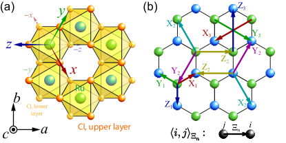
Figure 1: (a) Simplified schematic of the lattice structure of monolayer α-RuCl_3, which is a honeycomb lattice of edge-sharing RuCl_6 octahedrons. Both the chemical frame $\displaystyle xyz$ and the crystallographic frame $\displaystyle abc$ are indicated in the figure. The Cl triangular lattices are actually slightly distorted. (b) Labels of bond types in the hopping term of the Hamiltonian. The blue (green) spheres represent the $\displaystyle A$ ($\displaystyle B$) sublattice of the Ru honeycomb lattice. The notation for the hopping parameters $\displaystyle\left\langle{i,j}\right\rangle_{\Xi_{n}}$ relates panel (b) to terms retained in the hopping Hamiltonian.

In α-RuCl_3, each Ru^3+ ion is at the center of an octahedron formed by 6 Cl^- ions, as shown in Fig. 1 (a). The octahedral crystal field splits the 5 $\displaystyle 4d$ orbits of Ru atom into 3 $\displaystyle t_{2g}$ orbits and 2 $\displaystyle e_{g}$ orbits, with the latter’s energy higher by several eV, allowing us to confine our attention to the degrees of freedom within the $\displaystyle t_{2g}$ space. The $\displaystyle t_{2g}$ orbits are stretched along the coordinate planes of the $\displaystyle xyz$ coordinate system shown in Fig. 1 (a), which differs from the crystallographic $\displaystyle abc$ frame by an orthogonal transformation of basis $\displaystyle\begin{pmatrix}\hat{a}&\hat{b}&\hat{c}\end{pmatrix}=\begin{pmatrix}\hat{x}&\hat{y}&\hat{z}\end{pmatrix}\mathbf{Q}$, where

$$\mathbf{Q}=\frac{1}{\sqrt{6}}\begin{pmatrix}1&-\sqrt{3}&\sqrt{2}\\ 1&\sqrt{3}&\sqrt{2}\\ -2&0&\sqrt{2}\end{pmatrix}.$$ (1)

In the insulating case, 5 electrons are present in the 6-dimensional $\displaystyle t_{2g}$ space on each site so it is more convenient to use a hole representation. We adopt the model Hamiltonian from Ref. Winter et al. (2016):

$$H=H_{\rm int}+H_{\rm SOC}+H_{\rm TB}.$$ (2)

The interaction part $\displaystyle H_{\rm int}$ is purely on-site and of Kanamori-type Georges et al. (2013):

$$\begin{array}[]{c}H_{\rm int}=\frac{1}{2}\sum_{i,\xi\eta,\sigma\sigma^{\prime}}\left(U^{\prime}h_{i,\xi\sigma}^{\dagger}h_{i,\eta\sigma^{\prime}}^{\dagger}h_{i,\eta\sigma^{\prime}}h_{i,\xi\sigma}\right.\\ \left.+J_{H}h_{i,\xi\sigma}^{\dagger}h_{i,\xi\sigma^{\prime}}^{\dagger}h_{i,\eta\sigma^{\prime}}h_{i,\eta\sigma}+J_{H}h_{i,\xi\sigma}^{\dagger}h_{i,\eta\sigma^{\prime}}^{\dagger}h_{i,\xi\sigma^{\prime}}h_{i,\eta\sigma}\right),\end{array}$$ (3)

where $\displaystyle i$ labels the honeycomb sites, $\displaystyle\xi,\eta=yz(x),xz(y),xy(z)$ label the atomic $\displaystyle t_{2g}$ orbits and $\displaystyle\sigma,\sigma^{\prime}=\uparrow,\downarrow$ label spin. $\displaystyle h_{i,\xi\sigma}^{\dagger}$ ($\displaystyle h_{i,\xi\sigma}$) creates (annihilates) a hole with spin $\displaystyle\sigma$ on the orbit $\displaystyle\xi$ of site $\displaystyle i$. Note that this expression is equivalent to the one given in Ref. Winter et al. (2016) with $\displaystyle U^{\prime}=U-2J_{H}$, where $\displaystyle U$ represents the Coulomb interaction strength and $\displaystyle J_{H}$ is the Hund’s coupling amplitude.

In the spin-orbital coupling (SOC) term

$$H_{\rm SOC}=\lambda\sum_{i,\xi\eta}\left(\bm{L}_{{\rm eff},\xi\eta}\cdot\SS_{\sigma\sigma^{\prime}}\right)h_{i,\xi\sigma}^{\dagger}h_{i,\eta\sigma^{\prime}},$$ (4)

the elements of the effective orbital angular momentum operator are $\displaystyle L_{{\rm eff},\xi\eta}^{\mu}=-i\epsilon_{\mu\xi\eta}$, $\displaystyle\mu,\xi,\eta=x,y,z$ and $\displaystyle\epsilon_{\mu\xi\eta}$ is the Levi-Civita symbol. The spin vector operator $\displaystyle\SS$ is half of the Pauli matrix vector.

The spin-independent tight-binding (TB) part

$$H_{\rm TB}=-\sum_{ij,\xi\eta,\sigma}T_{ij}^{\xi\eta}h_{i,\xi\sigma}^{\dagger}h_{j,\eta\sigma}$$ (5)

consists of a crystal field (CF) contribution $\displaystyle H_{\rm CF}$ ($\displaystyle i=j$) and a hopping contribution $\displaystyle H_{\rm hop}$ ($\displaystyle i\neq j$). $\displaystyle H_{\rm CF}$ exists due to the deviation of the true crystal field from a perfect octahedral field, while $\displaystyle H_{\rm hop}$ includes up to the third-nearest neighbor hopping. For bond $\displaystyle\left\langle{i,j}\right\rangle_{\Xi_{n}}$, $\displaystyle T_{ij}^{\xi\eta}=T_{\Xi_{n}}^{\xi\eta}$ where $\displaystyle\Xi=X,Y,Z$, $\displaystyle n=1,2,3$ and the definitions of all bond types $\displaystyle\Xi_{n}$ are illustrated in Fig. 1 (b). In the presence of time-reversal ($\displaystyle\mathcal{T}$), spatial inversion ($\displaystyle\mathcal{I}$), in-plane 3-fold rotations ($\displaystyle C_{3}$) and a 2-fold rotation symmetry about the $\displaystyle b$ axis ($\displaystyle C_{2b}$), the hopping matrices are constrained to the forms

$$\begin{array}[]{c}\mathbf{T}_{Z_{1}}=\begin{pmatrix}t_{1}&t_{2}&t_{4}\\ t_{2}&t_{1}&t_{4}\\ t_{4}&t_{4}&t_{3}\end{pmatrix},\quad\mathbf{T}_{Z_{2}}=\begin{pmatrix}t_{1}^{\prime}&t_{2}^{\prime}&t_{4^{\prime}}^{\prime}\\ t_{2^{\prime}}^{\prime}&t_{1}^{\prime}&t_{4}^{\prime}\\ t_{4}^{\prime}&t_{4^{\prime}}^{\prime}&t_{3}^{\prime}\end{pmatrix},\\ \mathbf{T}_{Z_{3}}=\begin{pmatrix}t_{1}^{\prime\prime}&t_{2}^{\prime\prime}&t_{4}^{\prime\prime}\\ t_{2}^{\prime\prime}&t_{1}^{\prime\prime}&t_{4}^{\prime\prime}\\ t_{4}^{\prime\prime}&t_{4}^{\prime\prime}&t_{3}^{\prime\prime}\end{pmatrix},\end{array}$$ (6)

with all entries real, and $\displaystyle\mathbf{T}_{X_{n}}$ and $\displaystyle\mathbf{T}_{Y_{n}}$ are obtained by successively applying the coordinate rotation $\displaystyle x\rightarrow y\rightarrow z\rightarrow x$ to $\displaystyle\mathbf{T}_{Z_{n}}$. The crystal field matrix is given by

$$\mathbf{T}_{ii}=\begin{pmatrix}0&\Delta&\Delta\\ \Delta&0&\Delta\\ \Delta&\Delta&0\end{pmatrix},$$ (7)

up to an irrelevant constant.

The parameters of this model have been extracted from bulk RuCl_3 ab initio results in Refs. Winter et al., 2016; Wang et al., 2017. We follow Ref. Winter et al., 2016 and use $\displaystyle U^{\prime}=1.8\rm eV$, $\displaystyle J_{H}=0.6\rm eV$ ($\displaystyle U=3\rm eV$) and $\displaystyle\lambda=0.15\rm eV$. In bulk systems, $\displaystyle C_{3}$ symmetry is violated by the $\displaystyle C2/m$ layer stacking arrangement. For the monolayer systems we study below, we recover $\displaystyle C_{3}$ symmetry by averaging the CF Hamiltonian over 3 directions. For nearest-neighbor hopping processes, we use the $\displaystyle Z_{1}$-bond parameters previously extracted from ab initio simulations of a suspended monolayer Biswas et al. (2019); for further neighbor hoppings we use $\displaystyle Z_{2}$- and $\displaystyle Z_{3}$-bond parameters from bulk systems.

III Results

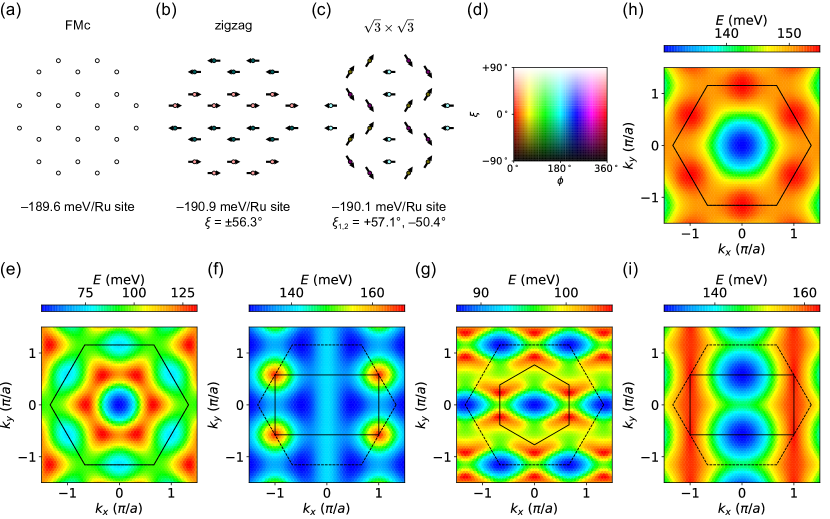
Figure 2: (a)-(c) The atomic magnetic moment configurations of (a) FMc, (b) zigzag and (c) $\displaystyle\sqrt{3}\times\sqrt{3}$ states. The arrows show the in-plane projections of the moments and the colors of the center spots represent the orientation of the moments, with the correspondence illustrated in legend (d), where $\displaystyle\phi$ is the azimuthal angle and $\displaystyle\xi$ is the canting angle, i.e. the elevation angle from the plane. Numerical values for energies and canting angles are provided below the figures. (For the $\displaystyle\sqrt{3}\times\sqrt{3}$ state the first canting angle is for the brighter sites and the second for the darker sites.) (e)-(g) The topography of the first conduction band of (e) FMc, (f) zigzag and (g) $\displaystyle\sqrt{3}\times\sqrt{3}$ states. (h)-(i) The topography of the first electronic conduction band of (h) FMc and (i) zigzag states with second- and third-nearest neighbor hopping amplitudes set to zero. In (f), (g) and (i), the dashed hexagon is the structural honeycomb lattice Brillouin zone (BZ) and the solid polygon is the magnetic BZ.

We perform self-consistent Hartree-Fock calculations on the monolayer model, limiting translational symmetry breaking by allowing magnetic unit cells with up to $\displaystyle 2\sqrt{3}\times 2\sqrt{3}$ honeycomb cells ($\displaystyle 12\times 2=24$ Ru sites). Given the supercell size we choose a variety of initial guesses for the density matrix that allow all other symmetries to be broken. We first discuss results obtained with the model parameter choices explained in the previous section. The low-energy magnetic configurations are shown in Figs. 2 (a)-(c) and the corresponding lowest electronic conduction bands are shown in Figs. 2 (e)-(g). Of all the extremal states we find, the zigzag state is the lowest in energy. The out-of-plane ferromagnetic (FMc) state is also competitive but only third lowest, exceeding the zigzag state by about $\displaystyle 1.3\rm meV$ per Ru atom. Between them in energy is a $\displaystyle\sqrt{3}\times\sqrt{3}$ state which has not been reported in previous work and has an energy that is higher than the zigzag state by $\displaystyle 0.84\rm meV$ per Ru atom. We do not find incommensurate spiral states, despite the strong dominance of $\displaystyle t_{2}$ which gives rise to a dominant Kitaev term in the spin model under the framework of second-order perturbation theory Winter et al. (2016). The findings that the ground state is a zigzag and that the FMc state is quite close in energy is consistent with experiment, and suggests that the model provides a reasonable description of RuCl_3.

To test how robust our results are against changes in model parameters, we also perform the self-consistent Hartree-Fock calculations excluding the second- and third-neighbor hopping integrals. As Figs. 2 (h)-(i) show, both the conduction bandwidth and the momentum-space location of the band bottom are strongly influenced by further-neighbor hopping. We will see in Sec. IV that the location of the conduction band minimum can have a profound influence on how the band interacts with a proximate layer of graphene. In the absence of further-neighbor hopping, the ground state remains zigzag, but the energy of FMc state is only $\displaystyle 0.11\rm meV$ per Ru site higher, and there is no longer a competitive $\displaystyle\sqrt{3}\times\sqrt{3}$ solution. The $\displaystyle\sqrt{3}\times\sqrt{3}$ state is absent even if we restore the further-neighbor hoppings to 80% of their original values, indicating that the state is fragile.

In summary we see that further-neighbor hopping helps to stabilize the zigzag state, and that it plays an important role in the band structure. We see in the following section that these relatively minor changes in electronic structure have a qualitative influence on how a RuCl₃ layer interacts with a graphene layer.

IV Hybridization with Graphene

The influence of an adjacent insulating van der Waals ferromagnet layer on the electronic structure of graphene is normally modeled by adding an exchange term to the graphene Hamiltonian, which spin-splits its bands. If the adjacent layer is AFM, as in the RuCl₃ case, the influence of oppositely directed moments tends to cancel because electrons in a small graphene Fermi pocket tend to average over atomic length scales. The situation can be more complex, however, when there is charge transfer between graphene and the van der Waals magnet, something that is known to occur Rizzo et al. (2020); Wang et al. (2020) in the RuCl₃ case. In discussing the electronic structure of the graphene/RuCl_3 system we recognize that although the 2D materials share a triangular Bravais lattice, they have very different Bravais lattice constants ($\displaystyle a_{\rm G}=2.46\text{\AA}$ for the graphene layer and $\displaystyle a_{\rm R}=5.8\text{\AA}$ for the RuCl₃) and their relative orientations are normally uncontrolled. In the rest of this section, we first model the interlayer coupling and then analyze its influence on the electronic structure of the combined system.

We assume a spin-conserving tunneling amplitude $\displaystyle T_{\xi}(\bm{r})$ from $\displaystyle t_{2g}$ $\displaystyle d$-orbital $\displaystyle\xi$ in RuCl_3 to the $\displaystyle p_{c}$ orbital in graphene that is some function of the difference $\displaystyle\bm{r}$ between the lateral 2D positions of the atoms in question. At this point we do not specify the concrete form of the function $\displaystyle T_{\xi}(\bm{r})$. Later on we will see that a model can be constructed from a small number of phenomenological parameters related to these functions.

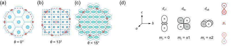
Figure 3: (a)-(c) Schematics of isolated graphene (red) and RuCl_3 Fermi surfaces (light blue, blue or green) and their reciprocal-lattice replicas for (a) FMc, (b) zigzag and (c) $\displaystyle\sqrt{3}\times\sqrt{3}$ magnetic states. These figures roughly assume that the electron charge transfer from graphene to RuCl_3 is $\displaystyle 0.04e$ per Ru atom ($\displaystyle 0.007e$ per carbon atom, $\displaystyle 2.7\times 10^{13}\rm cm^{-2}$ Rizzo et al. (2020)). The illustrated twist angle of the graphene lattice with respect to RuCl_3 is indicated below each figure. The bands of the FMc and $\displaystyle\sqrt{3}\times\sqrt{3}$ states are non-degenerate whereas those of the zigzag state are doubly degenerate. It follows that for the FMc and $\displaystyle\sqrt{3}\times\sqrt{3}$ states the total Fermi surface area per magnetic BZ is double that of graphene, whereas that of the zigzag state is the same. However, the fraction of $\displaystyle\bm{k}$-space that is within a replica Fermi surface is equal in the FMc and zigzag cases, because the zigzag BZ is half as large, while the replicated $\displaystyle\sqrt{3}\times\sqrt{3}$ Fermi surfaces occupy an area that is three times larger because the BZ area of this state is $\displaystyle 1/3$ of that of FMc. In (b), the intersecting Fermi surfaces are highlighted by small dashed boxes, and their replicas in the first BZ of RuCl_3 are also shown. (d) Schematics of some $\displaystyle d$ orbits in the $\displaystyle abc$ frame of RuCl_3 and the $\displaystyle p_{c}$ orbit of graphene.

Following a procedure similar to that used in the derivation of Bistritzer-MacDonald model of twisted bilayer graphene Bistritzer and MacDonald (2011), we obtain the following expression for interlayer tunneling between Bloch states in the two layers:

$$\begin{array}[]{c}\left\langle{{\rm G},\alpha\sigma\bm{k}}\middle|{H}\middle|{{\rm R},\beta\xi\sigma^{\prime}\bm{p}}\right\rangle=\delta_{\sigma\sigma^{\prime}}\times\\ \sum_{\bm{G}^{\rm G},\bm{G}^{\rm R}}w_{\xi}(\bm{k}+\bm{G}^{\rm G})\,e^{i\left(\bm{G}^{\rm G}\cdot\bm{\tau}_{\alpha}^{\rm G}-\bm{G}^{\rm R}\cdot\bm{\tau}_{\beta}^{\rm R}\right)}\,\delta_{\bm{k}+\bm{G}^{\rm G},\bm{p}+\bm{G}^{\rm R}},\end{array}$$ (8)

where $\displaystyle\alpha$ ($\displaystyle\beta$) labels the graphene (RuCl_3) sublattice, $\displaystyle\sigma,\sigma^{\prime}=\uparrow,\downarrow$ label spin, $\displaystyle\bm{G}^{\rm G}$ and $\displaystyle\bm{G}^{\rm R}$ are respectively reciprocal lattice vectors of the graphene and RuCl_3 layer, $\displaystyle\bm{\tau}_{\alpha}^{\rm G}$ ($\displaystyle\bm{\tau}_{\beta}^{\rm R}$) is the location of sublattice $\displaystyle\alpha$ ($\displaystyle\beta$) in a graphene (RuCl_3) unit cell, and

$$w_{\xi}(\bm{q})=\frac{1}{\sqrt{\Omega_{c}^{\rm G}\Omega_{c}^{\rm R}}}\int d^{2}\bm{r}T_{\xi}(\bm{r})e^{-i\bm{q}\cdot\bm{r}}$$ (9)

is proportional to the Fourier transform of the real-space tunneling function. $\displaystyle\Omega_{c}^{\rm G}$ and $\displaystyle\Omega_{c}^{\rm R}$ are the unit cell areas of graphene and RuCl_3, respectively. We see that the condition for Bloch states in the two layers to hybridize is that the two momenta should be equal when reduced to the BZ of one layer up to a reciprocal lattice vector of the other layer.

Because the separation between layers exceeds the atom size in either layer, $\displaystyle w_{\xi}(\bm{q})$ typically drops rapidly with $\displaystyle|\bm{q}|$. We are mainly interested in how hybridization with the magnetic insulators influences the transport properties of graphene, and therefore mainly interested in single-particle states with energies close to the graphene Fermi energy. Because the carrier density in graphene layer is relatively small when normalized per atom, its low energy electronic states lie at momenta close to the Dirac points $\displaystyle\pm\bm{K}^{\rm G}=\pm(4\pi/3a_{\rm G})(\cos\theta,\sin\theta)$. (Here $\displaystyle\theta$ is the orientation angle of graphene relative to that of RuCl_3.) For this reason we can replace $\displaystyle w_{\xi}(\bm{k}+\bm{G}^{\rm G})$ in Eq. 8 by $\displaystyle w_{\xi}(\bm{K})$, where $\displaystyle\bm{K}$ is the closest graphene BZ corner. Ab initio electronic structure calculations Biswas et al. (2019) suggest a typical hybridization strength $\displaystyle w_{\xi}(\bm{K})\sim 10\rm meV$. The RuCl₃ BZ momenta $\displaystyle{\bm{p}}$ that satisfy the $\displaystyle\delta$-function in Eq. (8) are those that are close to a corner when reduced to graphene’s BZ. We discuss the implications of these properties further below.

We discuss two limits of coupling between graphene’s near-Fermi surface states and RuCl_3 states. When the graphene state couples to a RuCl_3 state that is separated from the Fermi energy by an energy $\displaystyle\Delta E$ that is much greater than the hybridization scale $\displaystyle w_{\xi}(\bm{K})$, the hybridization can be treated perturbatively and gives rise to energy shifts that are $\displaystyle\sim w_{\xi}(\bm{K})^{2}/\Delta E$ and potentially spin-dependent as discussed further below. These spin-dependent energy shifts are the exchange interactions between graphene quasiparticles and the magnetic insulator spins mentioned above. On the other hand if a RuCl_3 state is within $\displaystyle w_{\xi}(\bm{K})$ around the Fermi energy, it will couple strongly to the graphene orbitals, creating avoided crossing gaps and reducing graphene orbital velocities to cause a significant drop in the conductivity of the system. Measurements of graphene transport properties therefore can be used to determine when the graphene Fermi surface intersects or nearly intersects the RuCl_3 Fermi surface.

The carriers of the Mott insulator RuCl_3 can be of either magnetic polarons or Fermi liquid character type depending on the level of doping Lee et al. (2006); Keimer et al. (2015); Koepsell et al. (2021). Here we assume that the location and shape of Fermi surface RuCl_3 is captured by rigid-band occupation of the conduction band obtained in Hartree-Fock calculations for the insulating state. As mentioned previously, those mean-field theory calculations do describe the competition between magnetic configurations reasonably accurately. As we explain below, the coupling between RuCl_3 and graphene layers can be strongly sensitive to their relative orientation $\displaystyle\theta$. If $\displaystyle\theta$ is not controlled when the bilayer device is fabricated, this sensitivity will lead to strongly device-dependent properties. On the other hand, in situ twist angle control Ribeiro-Palau et al. (2018); Inbar et al. (2023) could add to the power of graphene transport probes of insulating magnetic states. In our analysis we allow for arbitrary relative orientation between the layers.

As Figs. 3 (a)-(c) show, Fermi surface intersections do not occur for any relative twist angle when RuCl_3 is in the FMc state. In contrast, for the zigzag state, we estimate that they occur within the twist angle range $\displaystyle\theta\sim(17\pm 4)^{\circ}$. For the $\displaystyle\sqrt{3}\times\sqrt{3}$ state, intersections occur within both $\displaystyle(0\pm 5)^{\circ}$ and $\displaystyle(16\pm 6)^{\circ}$ orientation intervals. In general the larger the magnetic unit cell, the smaller the magnetic BZ, the denser the magnetic insulator Fermi surface $\displaystyle\bm{k}$ space replicas, increasing the chance that Fermi surfaces intersect. When the insulator has an ordered magnetic state, lower translational symmetry (larger magnetic unit cells) limits the ability of momentum conservation to restrict hybridization. We speculate that interlayer hybridization has a weaker effect in spin-liquid states because they do not break translational symmetry. The role of interlayer hybridization in graphene/Kitaev spin liquid heterostructures could be explored by generalizing earlier Kondo-Kitaev lattice model analyses Leeb et al. (2021); Jin and Knolle (2021) to the physically relevant case of incommensurate lattices, but this is outside the scope of the current study.

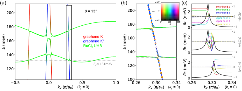
Figure 4: (a) Close up of an avoided crossing between strongly dispersing graphene and weakly dispersing RuCl_3 bands for the zigzag state of RuCl_3. As is clear from Fig. 3 (b), at orientation $\displaystyle\theta=13^{\circ}$ the Fermi surfaces of the two graphene valleys have a small intersection near $\displaystyle\bm{k}=0$ when mapped to the zigzag state magnetic BZ. For this illustration, we have taken the energy of graphene’s Dirac point to be $\displaystyle 650\rm meV$ higher than the upper Hubbard band bottom, $\displaystyle w_{0}=10\rm meV$, $\displaystyle w_{1}=5\rm meV$ and $\displaystyle w_{2}=3\rm meV$. We see that near RuCl_3’s BZ center, its states couple to both valleys of graphene. (b) An enlarged illustration of the avoided band crossing from the boxed region in (e). The dashed lines in (a) and (b) mark the position of the Fermi energy. The size of the spots in (b) represents the graphene fraction of the eigenstates, and the color represents the spin orientation of the graphene component of the eigenstate, using the color scale shown at the top right corner (and also in Fig. 2 (d)). The graphene spin splitting is largest close to the avoided crossing points, and the spin orientations of the spin-split states lie close to the $\displaystyle ab$ plane. (c) Plot of Kramers degeneracy splitting $\displaystyle\delta\epsilon$ and the expectation values of the graphene-projected spin Pauli matrices $\displaystyle\sigma_{\rm G}^{\mu}$ in the three spatial directions $\displaystyle\mu=a,b,c$. The upper, middle and lower panels correspond respectively to the upper two, middle two and lower two bands shown in (b). We see that close to the hybridization points, the spin splitting can be up to $\displaystyle\sim 3\rm meV$, while away from the hybridization points the exchange splitting of graphene energies rapidly goes down to $\displaystyle\sim 0.1\rm meV$ with the splitting of zigzag upper Hubbard bands even weaker. The spin-split graphene bands generally have almost in-plane spin orientations, which tend to stabilize at azimuthal angles close to $\displaystyle 36^{\circ}$ and $\displaystyle 216^{\circ}$ as one goes away from hybridization point.

There is an opportunity to reduce the number of free parameters that are relevant for hybridization by symmetry. This can be seen by noting that the $\displaystyle t_{2g}$ orbital wave functions, $\displaystyle\phi_{yz}(\bm{x})=yz\Phi(|\bm{x}|)$, $\displaystyle\phi_{xz}(\bm{x})=xz\Phi(|\bm{x}|)$ and $\displaystyle\phi_{xy}(\bm{x})=xy\Phi(|\bm{x}|)$, are linear combinations of the $\displaystyle c$-projected angular momentum $\displaystyle m_{c}$ eigenstates:

$$\begin{cases}\phi_{m_{c}=0}(\bm{x})=\frac{1}{\sqrt{3}}\left(c^{2}-\frac{a^{2}+b^{2}}{2}\right)\Phi(|\bm{x}|),\\ \phi_{m_{c}=\pm 1}(\bm{x})=\frac{(a\pm ib)c}{\sqrt{2}}\Phi(|\bm{x}|),\\ \phi_{m_{c}=\pm 2}(\bm{x})=\frac{(a\pm ib)^{2}}{2\sqrt{2}}\Phi(|\bm{x}|).\end{cases}$$ (10)

Here we use $\displaystyle\bm{x}$ to represent 3D position vectors to distinguish from 2D position vector $\displaystyle\bm{r}$. In a two-center approximation, $\displaystyle T_{m_{c}}(\bm{r})=T_{\left|{m_{c}}\right|}(\left|{\bm{r}}\right|)e^{im_{c}\theta_{\bm{r}}}$, implying that

$$w_{m_{c}}\left(\bm{q}\right)=i^{m_{c}}w_{\left|{m_{c}}\right|}(\left|{\bm{q}}\right|)e^{im_{c}\theta_{\bm{q}}}.$$ (11)

In this way we are able to express interlayer coupling in terms of three real parameters $\displaystyle w_{m_{c}}=w_{m_{c}}(\left|{\bm{K}^{\rm G}}\right|)$, where $\displaystyle m_{c}=0,1,2$. We expect the energy hierarchy between them to be $\displaystyle|w_{0}|>|w_{1}|>|w_{2}|$ since from the schematic shown in Fig. 3 (d), larger $\displaystyle\left|{m_{c}}\right|$ orbitals orbit extend more along $\displaystyle ab$ plane and less along $\displaystyle c$ axis, implying that the real-space tunneling function $\displaystyle T_{m_{c}}(\bm{r})$ has broader range but overall smaller absolute value, and thus that the momentum-space tunneling function $\displaystyle w_{m_{c}}(\bm{q})$ has narrower range. In Fig. 4 (a) we take $\displaystyle w_{0}=10\rm meV$, $\displaystyle w_{1}=5\rm meV$ and $\displaystyle w_{2}=3\rm meV$ and graphene Dirac velocity $\displaystyle\hbar v_{F}=7\rm eV\cdot\text{\AA}$. These numbers have only a qualitative justification, especially when the possible importance of hopping between metal ions via Cl p-bands is recognized. Their order of magnitude is chosen to reproduce the typical size of ab initio band hybridization gaps.

In the decoupled limit, both the graphene and the zigzag state RuCl_3 bands are doubly degenerate. Both degeneracies can be viewed as Kramer’s degeneracies protected by $\displaystyle\bm{k}$-preserving $\displaystyle\mathcal{I}\mathcal{T}$ symmetry, where $\displaystyle\mathcal{I}$ is the 3D spatial inversion operator and $\displaystyle\mathcal{T}$ is the time-reversal operator. When the coupling between the two layers is turned on, the band degeneracies of both materials are weakly lifted. This observation is consistent with the fact that placing graphene on top of a RuCl_3 layer breaks overall $\displaystyle\mathcal{I}\mathcal{T}$ symmetry. Because its tunneling amplitudes are odd under reflection through a plane midway between the two layers, the $\displaystyle w_{1}$ contribution dominates the Kramers violation. Away from the hybridization points, the exchange splitting of the graphene bands quickly drops to values $\displaystyle\sim 0.1\rm meV$, far smaller than in a graphene/FM insulator heterostructure. This finding is consistent with our expectation that the exchange coupling effects in graphene are extremely small when the magnetic layer does not have a net moment. At the hybridization points, both spin channels of the graphene band are gapped and the spin splitting increases to $\displaystyle 2\sim 3\rm meV$. We therefore expect that a reduction in overall electrical conductivity will accompany Fermi surface intersections, even when the magnetic insulator is in an AFM state. Note that in the coupled bilayer system the total spin-magnetization of the combined system in nominally AFM systems will generically be non-zero because of the small splitting of polarized states at the Fermi energy.

The case in which the magnetic layer has aligned spins, either in its ground state as in the FM insulator CrI_3 Tseng et al. (2022) or due to field alignment, is distinct. The bands of the isolated magnetic layer are then non-degenerate and spin-polarized, so that only one graphene spin-component is influenced by hybridization. For example in the case of graphene/CrI_3, the spin-degenerate graphene $\displaystyle\pi$-bands cross Cardoso et al. (2018, ) a non-degenerate band of the magnetic insulator. When hybridization is included, only one graphene spin channel is gapped. Under these circumstances we expect spin-polarized electronic transport, with the conductivity of the graphene spin-component that is present in the conduction band of the magnetic layer suppressed. We predict, based on our electronic structure model, that this suppression is anomalously weak in spin-aligned RuCl_3, independent of twist angle, because of the absence of Fermi surface intersections illustrated in Fig. 3(a). In contrast, graphene spin-transport would be expected to be strongly spin-polarized in graphene/RuCl_3 if the fragile $\displaystyle\sqrt{3}\times\sqrt{3}$ magnetic state were stable, since this configuration has Fermi surface intersections at many twist angles.

We note that in some spin-aligned materials, including in FM CrI_3, the conduction band quasiparticles have the majority spin, differing from valence band states via orbital instead of spin quantum numbers. This is unlike the RuCl_3 case, in which the conduction band states can be viewed as forming an upper Hubbard band with spins opposite to those of the occupied valence band states. In the hypothetical case in which the combined system Kramer’s degeneracy is protected by $\displaystyle C_{2}\mathcal{T}$ symmetry, where $\displaystyle C_{2}$ is the in-plane two-fold rotation, interlayer coupling would not break Kramer’s degeneracy and transport would not be spin-dependent, but conductivity suppression will still accompany Fermi surface intersections.

V Summary and Discussion

In this work we have analyzed how the electronic properties of an adjacent graphene layer can be used to probe the magnetic state of 2D magnetic insulators, focusing on the Kitaev material RuCl_3 as a typical interesting example. We assume that the Dirac point of graphene lies outside the band gap of the insulator so that charge transfer occurs between the two single-layer 2D systems. Charge transfer occurs in Cr, Fe and Ru trihalides Zhang et al. (2018); Cardoso et al. (2018); Rizzo et al. (2020); Wang et al. (2020); Li et al. (2020); Tseng et al. (2022); Lyu et al. (2022); Cardoso et al. , and we believe that it is likely to be common. We predict that hybridization of the materials can lead to sizable magneto-resistance that is sensitive to the magnetic configuration of the insulator and to the relative orientation of the two layers.

Our specific predictions rely on a mean-field model description of both graphene and the doped 2D magnetic insulator. We find that Hartree-Fock theory applied to a simple but realisitic model Hamiltonian is able to predict the relative stability of different magnetic configurations of the single-layer Mott insulator RuCl_3. In agreement with earlier work Sarikurt et al. (2018); Gerber et al. (2020); Souza et al. (2022), we find that the ground state is a zigzag AFM but the out-of-plane FM state is also competitive – explaining the weak fields required to achieve spin alignment in bulk RuCl_3. We also find a state with a $\displaystyle\sqrt{3}\times\sqrt{3}$ magnetic cell that is metastable in a narrow range of model parameters but is very fragile.

Our explicit calculations have a number of deficiencies. First of all, we do not account for many-body fluctuations in Bloch state occupation numbers. These fluctuations can in principle Lee et al. (2006) eliminate the momentum-space occupation number discontinuities associated with the Fermi surfaces we have discussed. We do not, however, expect them to change the locations in momentum space that have high spectral weight near the Fermi energy. It follows that the conclusions of our mean-field analysis should, for the most part, be unaffected.

Secondly, we do not account for structural relaxation of the van der Waals bilayers. Atomic position readjustments will be larger in the RuCl₃ layer, which is not as stiff as the graphene layer, but we do not expect them to be large because interlayer interactions are weak. The RuCl_6 crystal field in isolated monolayer RuCl_3 is close to the ideal octahedral form, as can be seen from the relatively small values of $\displaystyle\Delta$ and $\displaystyle t_{4}$ in the model Biswas et al. (2019). We expect the relaxations of the Cl ions closer to the graphene layer to distort the metal coordination further from the octahedral ideal than in the isolated layer case, which could increase the contribution of Ru–Cl–Ru indirect hopping to the nearest-neighbor hopping parameters Winter et al. (2016). Reference Gerber et al., 2020 predicts that the effect of graphene favors the zigzag state, and also makes other AFM states more competitive.

We analyze the coupled bilayer within a mean-field framework by considering the effect of interlayer hybridization as a weak perturbation. For RuCl_3 the hybridization energy scale is estimated to be $\displaystyle w\sim 10$ meV, smaller than the bandwidth of either material. We argue that its influence on electronic properties is sensitive primarily to the presence or absence of intersections between the Fermi surfaces of the two materials when the magnetic material Fermi surface is plotted in an extended-zone scheme as in Fig. 3. Intersections between Fermi surfaces will always suppress the graphene conductivity, and in the case of spin-aligned magnetic insulators, make it spin-dependent. Intersections occur for both zigzag and $\displaystyle\sqrt{3}\times\sqrt{3}$ states of RuCl_3 over certain ranges of relative orientation angle between the two layers. In the zigzag case both spin channels of graphene are gapped. Spin-splittings $\displaystyle\delta\epsilon\lesssim w$ occur only at those points in momentum space where strong hybridization occurs. Upon moving away from band crossing points, the symmetries of the isolated layers are gradually recovered and the spin-splitting is very small. On the other hand for out-of-plane spin-aligned magnetic configurations, weak exchange splitting occurs throughout momentum space. In the case of RuCl_3, these weakly momentum dependent exchange splittings are the main consequence of hybridization since Fermi surface intersections do not occur.

We have discussed mainly the influence of coupling between layers on lateral transport within the graphene layers, but our theory can also be used to address vertical transport. However, it may not be clear exactly how this quantity is best measured because it may be difficult to contact the magnetic insulator layers. The more interesting observable is, perhaps, transport between graphene layers through a magnetic layer. For both vertical and lateral transports, fabrication of graphene/magnetic-insulator devices with in situ twist-angle-control Ribeiro-Palau et al. (2018); Inbar et al. (2023) would greatly enhance the power of transport probes, because it would allow the Fermi surface of the magnetic insulator to be mapped out.

Although we have focused on the influence of the magnetic state on graphene transport, which is more readily observable, there must also be inverse effect in which hybridization tilts the competition between magnetic states. On general grounds interlayer hybridization will lower energy and therefore favor ordered states that have large Fermi surface overlaps with graphene. This effect will be small however and can only be the deciding factor if the pre-hybridization energies of the competing states are very close. It should also favor ordered magnetic states over spin-liquid states, in which inter-layer hybridization is likely suppressed by quasiparticle fractionalization. Like all hybridization effects, the influence on magnetic state competitions can be enhanced by applying pressure to narrow the van der Waals layer separations. This strategy might be readily simple to purse experimentally. Interesting future directions also include explorations on how transport properties of graphene can probe the magnons of ordered states Yang et al. (2023) and the magnetic polarons of the doped Mott-insulating states of substrate.