Spread Complexity in free fermion models

Abstract

We study spread complexity and the statistics of work done for quenches in the three-spin interacting Ising model, the XY spin chain, and the Su-Schrieffer-Heeger model. We study these models without quench and for different schemes of quenches such as sudden quench and multiple sudden quenches. We employ the Floquet operator technique to investigate all three models in the presence of time-dependent periodic driving of parameters. In contrast to the sudden quenched cases, the periodically varying parameter case clearly shows non-analytical behaviour near the critical point. We also elucidate the relation between work done and the Lanczos coefficient and how the statistics of work done behave near critical points.

I Introduction

The notion of complexity for a quantum state has become a well-known probe of interesting physical phenomena like quantum chaos and quantum phase transitions sachdev . There are several variants of complexity currently available in the literature Chapman:2021jbh . Perhaps the most studied example is the Nielsen complexity, which measures the least number of unitary operations to construct a target state from a given reference state myers ; khan ; praj ; gautam ; Bhattacharyya:2018bbv ; Jaiswal:2020snm . More recently, Balasubramanian et al. balas came out with the concept of spread complexity (SC), which will be the focus of this work.

Recall that in a geometrical framework, the computation of Nielsen complexity reduces to finding the geodesic connecting the target and reference states. For this, we require to make specific choices of the unitary gates, their penalties, and cost functionals. These requirements might raise legitimate concerns as to which features of the quantum system the complexity actually depends on. Therefore, one has to look for a more general form of complexity, which was addressed recently in balas , where the concept of SC of a quantum state under a unitary evolution was introduced. Roughly, the SC measures the spread of wave function over some fixed basis. Suppose that we start with an initial state and allow it to spread with time over a given basis; then, one can define SC by minimizing the cost associated with spread over all possible basis. Importantly, it was proved in balas that the basis set which minimises the cost associated with the wavefunction spreading is nothing but the Krylov basis, which can be constructed by using the standard Gram-Schmidt orthogonalization process starting from the initial state parker ; Viswanath ; Lanczos . Unlike Nielsen complexity, SC requires only the reference and target states, given the Hamiltonian of the system. The algorithm for its construction is also computationally efficient. Given these advantages, SC has therefore received the attention of late gcaptua ; pratik ; kcaptua ; parker ; Lanczos ; shir ; captua ; Nizami ; sayantanb ; sayantan . Among these works, captua computed SC for the Su-Schrieffer-Heeger (SSH) model and found that, in a quench protocol, SC can distinguish the different topological phases of the SSH system. This result was also further supported in a later work kcaptua , where the SC was used to differentiate the two topological phases of a Kitaev chain, which establishes the SC as a standard probe of the quantum phase transition.

In line with the above discussion, in this paper, we are interested in studying the nature of SC of non-equilibrium dynamics in many-body quantum systems. Recall that a system can be taken out of the equilibrium in several ways: by applying a driving field or by pumping energy and particles into the system, etc. Here we will study the behaviour of SC in such non-equilibrium dynamics by changing one of the parameters of the system, i.e., by employing a quantum quench quan ; venuti ; polko . In this paper, we calculate the SC for three paradigmatic models: the transverse XY spin chain, the Ising model with three-spin interactions, and the Su-Schrieffer-Heeger model (SSH), where the evolution is assumed to be under both time-dependent and time-independent Hamiltonians. We start with a brief discussion on the construction of the Krylov basis and the procedure to calculate the associated Lanczos coefficients via the geometric method, first introduced in gcaptua . Then we explain the dynamics of SC for a single sudden quench, multiple sudden quenches, and periodic driving for all three spin chains. In particular, in a time-dependent scenario, we calculate the SC by periodically changing the parameter over the stroboscopic time.

Finally, recalling that a quantum quench is analogous to a classical thermodynamic transformation and is characterised by usual thermodynamic quantities, such as the work done on the system, entropy produced, and heat exchanged kurchan ; talkner , here we compute the average and the variance of the work done on the system for a quantum quench silva . We also discuss the relation between the Lanczos coefficients and the average and the variance of the distribution of the work done in these systems.

Let us start with a brief discussion of the construction of the Krylov basis, which plays a main role in computation and the subsequent definition of SC following balas ; gcaptua ; kcaptua . Consider a general quantum state $\ket{\psi(s)}$, related to another one by the unitary transformation $\ket{\psi(s)}=\exp(-iHs)\ket{\psi(0)}$. We call $\ket{\psi(0)}$ as the reference state and $\ket{\psi(s=1)}$ as the target state. The parameter $s$ is the circuit parameter that connects the reference and target states, running from $0$ to $1$. To calculate the SC, the target state is expanded in a given basis $\{\ket{\psi_{n}}\}$

$$\ket{\psi(s)}=\sum_{n=0}^{\infty}\frac{(is)^{n}}{n!}\ket{\psi_{n}}~{},$$ (1)

where $\ket{\psi_{n}}=H^{n}\ket{\psi(0)}$, $H$ being the Hamiltonian generating the above unitary transformation. The Gram-Schmidt procedure is applied to these states to obtain a orthonormal basis ($\mathcal{K}=[\ket{K_{n}}$,$n$=0,1,2….]). These basis vectors form a subspace of the Hilbert space, and have a dimension generally less than that of the Hilbert space. To quantify how much $\ket{\psi(0)}$ spreads over the Hilbert space while evolving under a given Hamiltonian, we consider the following cost function for an arbitrary orthonormal basis $\mathcal{B}=\ket{B_{n}}$

$$\mathcal{C_{\mathcal{B}}}(s)=\sum_{n}n|\bra{\psi(s)}\ket{B_{n}}|^{2}~{},$$ (2)

and then subsequently minimise it over all choices of basis. Spread complexity is then defined as

$$\mathcal{C}(s)=\textit{min}_{\mathcal{B}}\mathcal{C_{\mathcal{B}}}(s)~{}.$$ (3)

The Hamiltonian in the Krylov basis is tridiagonal, i.e.,

$$H\ket{K_{n}}=a_{n}\ket{K_{n}}+b_{n}\ket{K_{n-1}}+b_{n+1}\ket{K_{n+1}}~{},$$ (4)

where the coefficients $a_{n},b_{n},b_{n+1}$ are known as the Lanczos coefficients. Similarly, the evolved state can be expanded in terms of the Krylov basis as

$$\ket{\psi(s)}=\sum_{n}\psi_{n}(s)\ket{K_{n}}~{},$$ (5)

and it can be checked that the evolved state satisfies the following discrete Schrodinger equation

$$i\partial_{s}\psi_{n}(s)=a_{n}\psi_{n}(s)+b_{n}\psi_{n-1}+b_{n+1}\psi_{n+1}$$ (6)

It was proved in balas , when evaluated in the Krylov basis, the cost defined in Eq. (2) becomes minimum, and hence the SC is defined as

$$\mathcal{C}(s)=\sum_{n}n|\psi_{n}(s)|^{2}~{}.$$ (7)

With this brief introduction, we now move to the main part of the paper and consider SC in different free fermion models.

II Three spins interacting transverse Ising model

The Hamiltonian of the transverse Ising model with three spin interactions is given by Kopp ; threediva :

$$\mathcal{H}=-\frac{1}{2}\Big{(}\sum_{i}\sigma^{z}_{i}\Big{[}h+J_{3}\sigma^{x}_{i-1}\sigma^{x}_{i+1}\Big{]}+J_{x}\sum_{i}\sigma^{x}_{i}\sigma^{x}_{i+1}\Big{)}~{},$$ (8)

Where $\sigma^{z}$ and $\sigma^{x}$ are Pauli matrices, $J_{x}$ is the strength of the nearest neighbour ferromagnetic interaction, and $J_{3}$ is the strength of three spin interactions. In the limit $J_{3}\to 0$, this model reduces to the standard transverse Ising model. Here, $J_{x}$ will be set to unity without loss of generality. Even in the presence of the three-spin interaction term, the Hamiltonian given by Eq. (8) is exactly solvable threediva . By a Jordan-Wigner(JW) transformation Jw1 ; Jw2 ; Jw3 and a Fourier transforms, we can map the Hamiltonian (8) into a free fermion model threediva .

$$H=-\sum_{k>0}(h+\cos{k}-J_{3}\cos{2k})(c^{\dagger}_{k}c_{k}+c^{\dagger}_{-k}c_{-k})+i(\sin{k}-J_{3}\sin{2k})(c^{\dagger}_{k}c^{\dagger}_{-k}+c_{k}c_{-k})~{}.$$ (9)

The Hamiltonian in Eq. (9) can be further diagonalized by using the Bogoliubov transformation, which yields the excitation spectrum

$$\epsilon_{k}=\sqrt{h^{2}+1+J_{3}^{2}+2h\cos{k}-2hJ_{3}\cos{2k}-2J_{3}\cos{k}}=|\vec{R}|.$$ (10)

From Eq. (10), it is seen that the energy gap vanishes at $h=J_{3}+1$ and $h=J_{3}-1$ for $k=\pi$, and $k=0$ modes, respectively. These two lines correspond to quantum phase transitions (QPTs) from paramagnetic to ferromagnetic ordered phases. The wave vector at which a minimum of $\epsilon_{k}$ occurs shifts from $k=0$ to $k=\pi$ when one crosses the line $h=J_{3}$. There is an additional phase transition at $h=-J_{3}$; this is an anisotropic transition. By taking $\frac{\partial\epsilon_{k}}{\partial k}=0$, we find out the values of wave vector $k$ at which Eq. (10) is minimum. Beside $k=0$ and $k=\pi$, we have

$$\cos{k}=\frac{h-J_{3}}{4hJ_{3}}~{},$$

At which the energy gap is minimum. By using the above value of $k$ in Eq. (10), one can see that $\epsilon_{k}$ is gapless at $h=-J_{3}$, and this line will intersect the $k=0$ line at $J_{3}=0.5$. Therefore, for $J_{3}<0.5$, the anisotropic transition cannot occur.
To study SC, we need to analyse the ground state and write it in terms of the Krylov basis. The Hamiltonian and ground state can be written in the following form (see Appendix A)

$$H=-\sum_{k>0}IR\cos\phi-\sum_{k>0}\Big{[}R\cos\phi J^{k}_{0}-iR\sin\phi(J^{k}_{+}-J^{k}_{-})\Big{]}~{},$$ (11)

where

$$\cos{\phi}=\frac{R_{3}}{R}~{},\qquad R_{3}=h+\cos{k}-J_{3}\cos{2k}~{},\qquad R_{2}=J_{3}\sin{2k}-\sin{k}~{},\qquad R=\sqrt{R_{2}^{2}+R_{3}^{2}}=|\vec{R}(k)|~{}.$$ (12)

Now it is easy to see that $J_{0}^{k}$, $J_{+}^{k}$, $J_{-}^{k}$, defined in Eq. (72) satisfy the commutation relations of $su(2)$ algebra, and hence, the Hamiltonian in Eq. (11) is actually an element of this algebra.

The ground state for a single momentum mode can be written as

$$\ket{\psi_{k}(s)}=e^{-i\frac{s\phi}{2}(J_{+}^{k}+J_{-}^{k})}\ket{\frac{1}{2},-\frac{1}{2}}_{k}$$ (13)

where $s=1$ corresponds to the target state. We now want to calculate the SC of creating this state starting from a suitable reference state. Here as the reference state, we make the most straightforward choice, i.e. fermion vacuum $\ket{0,0}$ which can be represented as $\ket{\frac{1}{2},-\frac{1}{2}}_{k}$. First, we write down the ground state in the following suitable form

$$\ket{\psi_{gs}}=\prod_{k>0}\cos{\frac{\pi-\phi}{2}}\exp\Big{[}e^{-i\frac{\pi}{2}}\tan{\frac{\pi-\phi}{2}}J_{+}^{k}\Big{]}\ket{j,-j}_{k}~{},$$ (14)

or

$$\ket{\psi_{gs}}=\prod_{k>0}\exp\Big{[}\frac{\pi-\phi}{2}e^{-i\frac{\pi}{2}}J_{+}^{k}-\frac{\pi-\phi}{2}e^{i\frac{\pi}{2}}J_{-}^{k}\Big{]}\ket{j,-j}_{k}~{},$$ (15)

where, in this case $j=\frac{1}{2}$.

Since the target state is a $SU(2)$ coherent state, the Krylov basis vectors are just gcaptua ; balas

$$\ket{K_{n}}=\ket{-j,j+n}=\sqrt{\frac{(2j-n)!}{n!(2j)!}}J_{+}^{n}\ket{j,-j}~{}.$$ (16)

Following a procedure similar to that of the one outlined in captua , we calculate the the SC for single momentum mode is to be

$$\mathcal{C}_{k}(s=1)=\left(\cos{\frac{\phi}{2}}\right)^{2}~{}.$$ (17)

Taking the continuum limit, we obtain the SC of the ground state as

$$\mathcal{C}=\frac{1}{2\pi}\int_{0}^{\pi}dk\left(\cos{\frac{\phi}{2}}\right)^{2}~{}.$$ (18)

In the continuum limit, we will work with the quantities per system size , so we suppress the factor $N$. And follow this notation throughout the paper. SC acts as a tool to probe quantum phase transitions has been discussed in captua ; kcaptua , via Eq. (18). Here, we take the derivative of Eq. (18) with respect to $h$ and plot the same in Fig. 1, and find that this shows a peak around critical points $J_{3}+1$ and $J_{3}-1$. There are three peaks for $J_{3}>0.5$, one of which corresponds to anisotropic transition $h=-J_{3}$.

II.1 Spread complexity evolution under a single quench

We now study the time dependence of the SC under a single sudden quench. We consider unitary time evolution of an initial state $\ket{\psi_{i}}$ (preferably eigenstate of an initial Hamiltonian $H_{i}$) under a different Hamiltonian $H_{f}(h_{f},J_{3f})$, which has parameter values different from the initial one. The evolved state at an arbitrary time is given by $\ket{\psi(t)}=\exp(-iH_{f}t)\ket{\psi_{i}}$, where we take $\ket{\psi_{i}}$ to be the ground state of initial Hamiltonian $H_{i}$ with parameters $(h_{i},J_{3i})$.

We first find out the return amplitude defined as $S=\braket{\psi(t)}{\psi_{i}}$. Since, $\ket{\psi_{i}}=\mathcal{D}(z_{i})\ket{j,-j}$, with

$$\mathcal{D}(z_{i})=\exp\Big{[}\frac{\pi-\phi_{i}}{2}e^{-i\frac{\pi}{2}}J_{+}-\frac{\pi-\phi_{i}}{2}e^{i\frac{\pi}{2}}J_{-}\Big{]}~{},$$ (19)

this is given by

$$S=\braket{\psi(t)}{\psi_{i}}=\bra{j,-j}\mathcal{D}^{\dagger}(z_{i})\exp{(iH_{f}t)}\mathcal{D}(z_{i})\ket{j,-j}~{}.$$ (20)

By using the Baker-Campbell-Hausdorff (BCH) formula, we can write down the analytical expression for the return amplitude to be

$$S=\cos(R_{f}t)-i\cos(\phi_{f}-\phi_{i})\sin(R_{f}t)~{}.$$ (21)

SC, in continuum limit is given by (see captua , and Appendix A)

$$\mathcal{C}(t)=\frac{1}{2\pi}\int_{0}^{\pi}\Big{(}1-|S|^{2}\Big{)}dk=\frac{1}{2\pi}\int_{0}^{\pi}\sin^{2}(\phi_{f}-\phi_{i})\sin^{2}(R_{f}t)dk~{}.$$ (22)

We plot the SC (Eq. (22)) in Fig. 3, where the red curve denotes the evolution when the initial value of parameters are at critical points, and the blue curve is when the final parameters are at critical points. The numerical values of the parameters for the red curve: $J_{3i}=0.4$, $J_{3f}=1$, $h_{f}=1.5$, and blue curve: $J_{3i}=1$, $J_{3f}=0.4$, $h_{i}=1.5$. From these plots, we see that at the late times, $\sin{(R_{f}t)}$ attain a constant value. It is clearly seen from Fig. 1 that there is no sign of QPT in the evolution of the SC, even when we take the parameters at critical points.

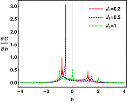
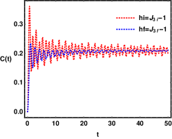
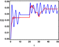
Figure 1: SC of the transverse Ising model with three spin interactions : (a)  Derivative of complexity with respect to $h$, (b)  SC evolution after a single quench, and (c)  SC after multiple quenches.

II.2 Spread complexity evolution after multiple quenches

In a multiple-quench scenario, we consider the succession of three quenches.

• We prepare the state of $H_{i}(h_{i},J_{3i})$ at $t=0$ and evolve it for $10$ using $U_{1}(t)=\exp[-iH_{f}(h_{f},J_{3f})t]$. By taking into account the overlap between evolved state and the initial state, we calculate the complexity using Eq. (22).

• In the next step, the initial state will be evolved by $U_{2}(t)=\exp[-iH_{i}(h_{i},J_{3i})t]\exp[-iH_{f}(h_{f},J_{3f})t_{1}]$, where $t_{1}=10$ and $10<t\leq 20$ and again by taking overlap of evolved state with an initial state, complexity can be calculated.

• In the last step, the initial state evolved by $U_{3}(t)=\exp[-iH_{f}(h_{f},J_{3f})t]\exp[-iH_{i}(h_{i},J_{3i})t_{2}]\exp[-iH_{f}(h_{f},J_{3f})t_{1}]$, where $t_{1}=10$, $t_{2}=20$ and $20<t\leq 50$, and the overlap of the initial state with the evolved state provide us complexity.

The results for the time evolution of the SC are depicted in Fig. 1. We consider behaviour around one of the critical points. The red curve shows the time evolution of SC when the final parameters are at a critical point and the blue curve when initial parameters are at critical points. In Fig. 1, we take $h=J_{3}-1$ as the critical point, and for the blue curve, the parameter values are $h_{i}=0.6$, $J_{3i}=1.6$, $h_{f}=1$, $J_{3f}=1.2$, while for the red curve, we take $h_{i}=1$, $J_{3i}=1.2$, $h_{f}=0.6$, $J_{3f}=1.6$. Analysing these results, we can see the amplitude of complexity depends on the initial and final values of the parameters and that, with increasing time, it attains steady values. Although the amplitude decreases by switching the value of parameters, there is no specific behaviour at the QPT. The behaviour of SC for multiple quenches is almost similar to the case of a single quench.

II.3 Spread complexity evolution with periodically driven field

In this section, we will study how the SC behaves when the system is driven by periodically varying fields russo ; vic ; shrad over stroboscopic time ($t=nT$, where $n\in\mathbb{Z}$). We replace $h=h(t)=\delta\cos{\omega t}+h_{c}$ in Eq. (8), $T$ is defined as the period for one oscillation $T=\frac{2\pi}{\omega}$. In this case, we use the invariant operator technique lai or the time-dependent unitary transformations Maam $i\frac{d}{dt}\ket{\psi(t)}=H(t)\ket{\psi(t)}$, $\hat{J_{0}}\ket{n}=J_{n}\ket{n}$. According to the well-known Lewis-Riesenfeld theory Lewis , the general solution of the Schrodinger equation is written as, $\ket{\psi(t)}=\sum_{n}c_{n}\exp(i\alpha_{n}(t))\ket{n,t}$, where $\ket{n,t}$ are eigenstate of the invariant operator $\mathcal{I}(t)\ket{n,t}=J_{n}\ket{n,t}$, with $\ket{n,t}=\hat{R}(t)\ket{n}$. This can also be written in the form

$$\ket{\psi(t)}=\hat{R}(t)\exp[-i\epsilon(t)J_{0}]\hat{R}^{\dagger}(0)\ket{\psi(0)}~{},$$ (23)

where we have denoted

$$\hat{R}(t)=\exp\Big{[}\frac{\gamma(t)}{2}\Big{(}\hat{J}_{+}e^{-i\beta(t)}-\hat{J}_{-}e^{i\beta(t)}\Big{)}\Big{]}~{},~{}\text{and}~{}~{}\gamma(t)=\tan^{-1}\Big{[}\frac{|(J_{3}\sin{2k}-\sin{k})|}{\cos{\omega t}+h_{c}+\cos{k}-J_{3}\cos{2k}}\Big{]}~{}.$$ (24)

We have to solve an auxiliary equation to find out the function $\gamma(t)$ and $\beta(t)$. Here we outline the computation of the return amplitude, as well as SC, while some of the relevant mathematical details are provided in Appendix D and Appendix E (see also lai ). To calculate SC we will express Eq. (23) in terms of the Krylov basis, which can be written by using the BCH formula Bch . And to calculate the SC, we take the initial state to be the ground state, i.e.,

$$\ket{\psi(0)}=\hat{R_{i}}\ket{j,-j}~{},~{}~{}\hat{R_{i}}=\exp\Big{[}-i\frac{\pi-\phi_{i}}{2}(J_{+}+J_{-})\Big{]}$$ (25)

where the explicit expression for $\phi_{i}$ is given by

$$\phi_{i}=\cos^{-1}\Big{[}\frac{(h_{c}+\cos{k}-J_{3}\cos{2k})}{\sqrt{(h_{c}+\cos{k}-J_{3}\cos{2k})^{2}+(J_{3}\sin{2k}-\sin{k})^{2}}}\Big{]}~{}.$$ (26)

The expression for the return amplitude for a single mode of momentum mode for general $j$ is given by

$$\mathcal{S}=\Big{[}\cos\Big{[}\frac{\gamma(0)-\gamma(t)}{2}\Big{]}\cos\big{[}\frac{\epsilon(t)}{2}\big{]}-i\cos\Big{[}\frac{\gamma(0)+\gamma(t)}{2}-\phi_{i}\Big{]}\sin\big{[}\frac{\epsilon(t)}{2}\big{]}\Big{]}^{2j}~{},$$ (27)

where

$$\epsilon(t)=\int_{0}^{t}\sqrt{(h(t^{\prime})+\cos{k}-J_{3}\cos{2k})^{2}+(J_{3}\sin{2k}-\sin{k})^{2}}dt^{\prime}~{}.$$

$\gamma(t)$ and $\hat{R}(t)$ are periodic, such that $\gamma(0)=\gamma(nT)$ and $\hat{R}(0)=\hat{R}(nT)$ Maam . Therefore, for periodic condition $\gamma(nT)=\gamma(0)=\gamma$, the SC for a single mode in free fermion $j-\frac{1}{2}$ case given by

$$\mathcal{C}_{k}=1-|\mathcal{S}|^{2}=\sin\Big{[}\frac{\epsilon(nT)}{2}\Big{]}^{2}\sin[\gamma-\phi_{i}]^{2}~{}.$$ (28)

As before, in the continuum limit, we obtain the total complexity to be

$$\mathcal{C}(s=1)=\frac{1}{2\pi}\int_{0}^{\pi}(1-|\mathcal{S}|^{2})dk~{}.$$ (29)

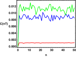
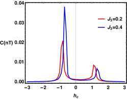
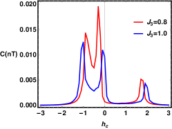
Figure 2: SC evolution in the case of periodically driven magnetic field (a) Complexity variation with number of oscillation, (b) Showing the two peaks that correspond to $h=J_{3}+1$ and $h=J_{3}-1$, (c) Showing the three peaks at $h=J_{3}+1$, $h=J_{3}-1$, $h=-J_{3}$.

We calculate complexity in Eq. (29) by using numerical integration method of Simpson- $\frac{1}{3}$ over $k$ from $(0,\pi)$ with step size $\frac{\pi}{1000}$, while doing the integration we fix $\delta=0.1$. We plot Eq. (29) with respect to number of oscillation $t=nT$, $T=\frac{2\pi}{\omega}$, $n\in\mathbb{Z}$. In Fig. 2 we have fixed $T=1000$ and vary the parameters $J_{3}$, $h_{c}$, as red: $J_{3}=0.2$, $h_{c}=0$, blue: $J_{3}=0.2$ , $h_{c}=1.1$, and green: $J_{3}=1$, $h_{c}=-1.1$. For the first cycle in Fig. 2, complexity growth is at its maximum; from then on, it begins to oscillate around an average value. We plot Eq. (29) with respect to $h_{c}$ by taking different values of $J_{3}$ and keeping $n=40$, $T=1000$. In Fig. 2 we take $J_{3}<0.5$, two peak correspond $h(nT)=J_{3}+1$ and $h(nT)=J_{3}-1$. In Fig. 2 we take $J_{3}>0.5$ and three peaks correspond to $h(nT)=J_{3}+1$, $h(nT)=J_{3}-1$, $h(nT)=-J_{3}$.

III XY Spin Model

In this section, we consider the spin-$\frac{1}{2}$ XY model placed in a magnetic field ($h$) pointed along $\hat{z}$ direction sharma . The Hamiltonian, in this case, is given by

$$H=-\sum_{j=1}^{N-1}\Big{[}\frac{1+\gamma}{2}\sigma_{j}^{x}\sigma_{j+1}^{x}+\frac{1-\gamma}{2}\sigma_{j}^{y}\sigma_{j+1}^{y}\Big{]}-\sum_{j=1}^{N}h\sigma_{j}^{z}~{}.$$ (30)

where $\gamma$ is the anisotropy parameter. This model and Three spin interaction TIM Eq. (8) are related by a duality transformation (see Appendix C). As before by performing successive Jordan-Wigner Jw1 ; Jw2 ; Jw3 and Fourier transformations we rewrite the above Hamiltonian as

$$H=-\sum_{k>0}(h+\cos{k})(c^{\dagger}_{k}c_{k}-c_{-k}c^{\dagger}_{-k})+\sum_{k>0}\big{[}i\gamma c^{\dagger}_{k}c^{\dagger}_{-k}-i\gamma c_{-k}c_{k}\big{]}~{}.$$ (31)

where now the energy gap is given by

$$\epsilon={\sqrt{(h+\cos k)^{2}+(\gamma\sin k)^{2}}}~{}.$$ (32)

Eq. (32) has extrema at $k=0$, $k=\pi$ and $\cos k_{o}=\frac{h}{-1+\gamma^{2}}$. Using these values of $k$ we can find out that Eq. (32) vanishes at $h=\pm 1$ and $\gamma=0$ (provided $|h|<1$). Therefore critical points for this system are $h=\pm 1$ and $\gamma=0$ for $h<1$.

Hamiltonian Eq. (31) can be written as an element of the $su(2)$ algebra as (see Appendix B for derivation)

$$H=\sum_{k>0}\Big{[}-2R\cos\phi J^{k}_{0}+iR\sin\phi J^{k}_{+}-iR\sin\phi J^{k}_{-}\Big{]}~{},$$ (33)

where we have defined

$$R(k)=\sqrt{R_{2}^{2}+R_{3}^{2}}~{},\qquad R_{2}=\gamma\sin{k},\qquad R_{3}=h+\cos{k}~{},\qquad\phi=\tan^{-1}\frac{|R_{2}|}{R_{3}}~{}.$$ (34)

The ground state of this model is of the same form as the three-spin interaction Ising model considered in the the previous section, i.e.

$$\ket{\psi_{gs}}=\prod_{k>0}\cos{\frac{\pi-\phi}{2}}\exp\Big{[}-i\tan{\frac{\pi-\phi}{2}}J_{+}^{k}\Big{]}\ket{\frac{1}{2},-\frac{1}{2}}_{k}~{},$$ (35)

This can be rewritten as

$$\ket{\psi_{gs}}=\prod_{k>0}\exp\Big{[}-i\frac{\pi-\phi}{2}J_{+}^{k}-i\frac{\pi-\phi}{2}J_{-}^{k}\Big{]}\ket{\frac{1}{2},-\frac{1}{2}}_{k}~{},$$ (36)

SC of formation of the ground state is given by the same formula in Eq. (18), with $\phi$, in this case, is the one given in Eq. (34). In Fig. 3, we have plotted the derivative of the SC in this case. As can be seen the derivative of SC shows non-analytical behaviour around $h=-1$ and $h=1$.

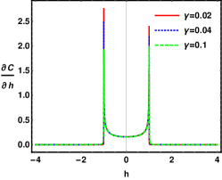
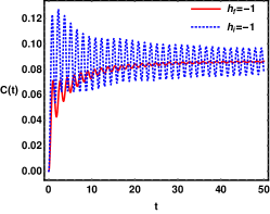
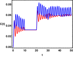
Figure 3: Spread complexity of the XY spin chain model : (a)  Derivative of complexity with respect to $h$. (b)  Complexity for a single quench. (c)  Complexity for multiple quenches

III.1 Spread Complexity evolution after a single quench

The quench protocol we consider here is the same as the one considered in the three-spin interactions Ising case. We consider a quench in this model such that the initial parameter values $h_{i}$, $\gamma_{i}$, are changed to new set of values $h_{f}$, $\gamma_{f}$. The SC can be calculated using the same procedure employed in the previous section and in the continuum limit the expression for the complexity is the same as in Eq. (22), i.e.

$$\mathcal{C}(t)=\frac{1}{2\pi}\int_{0}^{\pi}\sin^{2}(\phi_{f}-\phi_{i})\sin^{2}(R_{f}t)dk~{},$$ (37)

where the expression for $\phi_{f}$ and $\phi_{i}$ are determined by the formula for $\phi$ in Eq. (34).

In Fig. 3, we have plotted the complexity evolution after a single quench. We consider the case when parameters are at one of the critical points $h=-1$, where the red curve reflects the behaviour of final parameters at the critical point, and the blue curve represents when initial parameters are at the critical point. For red curve we choose the parameter values : $h_{i}=1.2$, $\gamma_{i}=0.4$, $h_{f}=-1.0$, $\gamma_{f}=0.2$, blue: $h_{i}=-1.0$, $\gamma_{i}=0.2$, $h_{f}=1.2$, $\gamma_{f}=0.4$.

III.2 Spread complexity evolution after multiple quenches

In multiple quenches, the quench protocol is the same as in three spin cases; here again, we consider one of the critical points $h=-1$. In Fig., 3 red curve reflects the behaviour for the final parameter at a critical point and blue for the initial parameter at a critical point. The parameter values are for the blue curve are : $h_{i}=-1$, $\gamma_{i}=0.05$, $h_{f}=1.2$, $\gamma_{f}=0.4$ and for red curve parameters are $h_{i}=1.2$, $\gamma_{i}=0.4$, $h_{f}=-1$, $\gamma_{f}=0.05$. For the case when the final parameters are at the critical point, complexity has fewer oscillations, and the magnitude of amplitude is less as compared to the case when the initial parameter is at a critical point. This can be understood from the expression of SC where we have time-dependent factor $(\sin(R_{f}t))^{2}$. Now since $R_{f}$ has the form of Energy gap $R_{f}=\sqrt{(h_{f}+\cos k)^{2}+(\gamma_{f}\sin k)^{2}}$, this attains minimum value at the critical points.

III.3 Spread complexity evolution with periodically driven field

In this case, we consider $h(t)=\delta\cos{(\omega t)}+h_{c}$ where time $t$ is discrete and measured in terms of integer $n$, $t=\frac{2n\pi}{\omega}$. The expression for the time evolved state is the same as Eq. (23) where now we have

$$\hat{R}(t)=\exp\Big{[}\frac{i\gamma(t)}{2}(J_{+}^{k}+J_{-}^{k})\Big{]}~{},~{}~{}~{}\text{and}~{}~{}\gamma(t)=\tan^{-1}\Big{[}\frac{\gamma\sin k}{h(t)+\cos k}\Big{]}~{}.$$ (38)

We calculate the evolution of the SC of this time evolved state with respect to an initial state $\ket{\psi(0)}=\hat{R_{i}}\ket{j,-j}$ (same as Eq. (25)) with

$$\phi_{i}=\cos^{-1}\Big{(}\frac{(h_{c}+\cos{k})}{\sqrt{(h_{c}+\cos{k})^{2}+(\gamma\sin{k})^{2}}}\Big{)}~{}.$$

With periodic boundary conditions, the expressions for the return amplitude for a single momentum mode and the complexity are the same as the ones in Eqs. (27) and (29) respectively, where now the expression for the time-dependent function $\epsilon(t)$ is given by

$$\epsilon(t)=\int_{0}^{t}\sqrt{(h(t^{\prime})+\cos{k})^{2}+(\gamma\sin{k})^{2}}dt^{\prime}~{}.$$ (39)

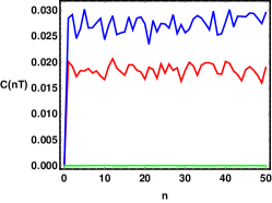
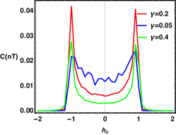
Figure 4: SC evolution with the periodic field in XY spin chain model : (a)  Variation with a number of oscillations. (b)  Variation with parameter $h_{c}$.

Fig. 4 shows the time evolution of the SC with $\delta=0.1$. In Fig. 4, we have plotted it with a number of oscillations $n$ with following values of the parameters: red $:\gamma=0.2$, $h_{c}=1$, blue $:$ $\gamma=0.4$, $h_{c}=-1$, and green: $\gamma=0.2$, $h_{c}=1.5$. On the other hand, in Fig. 4, we have plotted it with respect to $h_{c}$ by taking $n=40$, $T=1000$ in all three cases.

IV Su-Schrieffer-Heeger Model

The SC in the SSH model has been studied previously in captua in the context of a single quantum quench. Here we are interested in studying the SC in this model after multiple quenches and in the presence of a time-varying field. Physically speaking, it defines a 1D lattice with a two-atom sublattice structure in which the hopping amplitudes between the lattices are typically different.

Hamiltonian of the SSH model is given by :

$$H=t_{1}\sum_{i}(c_{Ai}^{\dagger}c_{Bi}+H.c)-t_{2}\sum_{i}(c_{Bi}^{\dagger}c_{A,i+1}+H.c)+\mu_{s}\sum_{i}(c_{Ai}^{\dagger}c_{Ai}-c_{Bi}^{\dagger}c_{Bi})$$ (40)

where $t_{1}$ is intra-cell hopping amplitude and $t_{2}$ is inter-cell hopping amplitude. $c_{Ai}$, $c_{Bi}$ represent fermions annihilation operators defined at site $i$ for sub lattice $A$ and $B$ respectively. We take $t_{1},t_{2}\geq 0$ and $\mu_{s}=0$. Depending on the values of parameters, there are two phases: non-topological phase for $t_{1}>t_{2}$ and topological phase for $t_{2}>t_{1}$. This model shows a QPT at $t_{1}=t_{2}$. Eq. (40) can be diagonalized using Fourier transform and Bogoliubov transformations.

In momentum space (with $\mu_{s}=0)$ the Hamiltonian can be rewritten as

$$H=\sum_{k}\Big{[}2R_{3}J_{0}^{k}+iR_{1}(J_{+}^{k}-J_{-}^{k})\Big{]}~{},$$ (41)

where

$$R_{1}=t_{1}-t_{2}\cos k~{},\quad R_{3}=t_{2}\cos k~{},\quad~{}~{}\text{and}~{}R(k)=|\vec{R}(k)|~{}.$$ (42)

The operators $J_{0}^{k},J_{\pm}^{k}$ satisfy the usual $su(2)$ Lie algebra, and future convenience we define

$$\sin\phi=\frac{|R_{1}|}{R}~{},\quad\cos{\phi}=\frac{R_{3}}{R}~{},\text{with}~{}~{}R=\sqrt{t_{1}^{2}+t_{2}^{2}-2t_{1}t_{2}\cos k}~{}.$$ (43)

The ground state of this model is given by

$$\ket{\psi_{g}}=\prod_{k>0}\cos^{2}\Big{(}\frac{\phi}{2}\Big{)}\exp\Big{[}-i\tan\Big{(}\frac{\phi}{2}\Big{)}\big{[}J_{+}^{k}e^{-i\psi_{k}}+J_{-}^{k}e^{i\psi_{k}}\big{]}\Big{]}\ket{\frac{1}{2},\frac{-1}{2}}_{k}~{}.$$ (44)

The SC of the ground state in the continuum limit is given by captua

$$\mathcal{C}=\frac{1}{\pi}\int_{0}^{\pi}dk\left(\sin{\frac{\phi}{2}}\right)^{2}~{}.$$ (45)

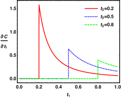
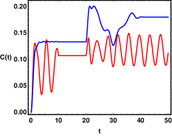
Figure 5: SC in SSH model : (a)  Derivative of complexity with parameter $t_{1}$ (b)  Evolution for multiple quenches.

IV.1 Complexity evolution after multiple quenches

The time evolved state after a quench is given by

$$\ket{\psi(t)}=e^{-iH_{f}t}\ket{\psi_{i}}~{}.$$ (46)

where $\ket{\psi_{i}}$ is the ground state defined in Eq. (44). Note that here $\phi=\phi_{i}$ and $\psi_{k}=0$, since $\mu_{s}=0$. In Fig. 5, we plot the derivative of spread complexity with respect to the parameter without quench case, and it clearly shows a non-analytical nature near the critical point $t_{1}=t_{2}$.

Return amplitude after a single quench can be written as captua

$$\mathcal{S}=\braket{\psi(t)}{\psi(0)}=\cos(R_{f}t)-i\cos(\phi_{f}-\phi_{i})\sin(R_{f}t)~{}.$$ (47)

The SC calculated from this return amplitude is given by

$$\mathcal{C}(t)=\int_{0}^{\pi}\frac{dk}{\pi}\sin^{2}(\phi_{f}-\phi_{i})\sin^{2}(R_{f}t)~{}.$$ (48)

In Fig. 5, we have plotted the behaviour of SC under multiple quenches, where the parameter values for the red curve: $t_{1i}=1=t_{2i}$, $t_{1f}=0.7$, $t_{2f}=1.5$, and for the blue curve: $t_{1i}=1.5$, $t_{2i}=0.7$, $t_{1f}=1=t_{2f}$, where $i$ subscript represents initial value and $f$ represents final value.

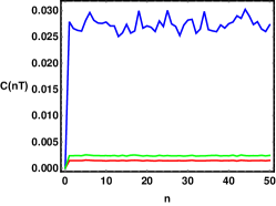
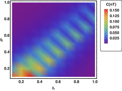
Figure 6: Spread complexity in case of periodic variation of parameter for SSH model : (a)  Complexity with number of oscillations (b)  Complexity with parameters

IV.2 Complexity evolution with periodically driven field

In presence of a periodically driven field we take $t_{1}=t_{1}-v(t)$ and $t_{2}=t_{2}+v(t)$, with $v(t)=\delta\cos(\omega t)$. The Return amplitude is once again of the same form as the one in Eq. (27), with

$$\gamma(t)=\arctan\Big{(}\frac{-|(t_{2}+v(t))\sin k|}{t_{1}-v(t)-(t_{2}+v(t))\cos k}\Big{)}~{},$$ (49)

and

$$\epsilon(t)=2\int_{0}^{t}\sqrt{[t_{1}-v(t^{\prime})-(t_{2}+v(t^{\prime}))\cos k]^{2}+[(t_{2}+v(t^{\prime}))\sin k}]^{2}dt^{\prime}~{}.$$ (50)

With periodic boundary conditions, in the continuum limit, the SC is given by

$$\mathcal{C}(nT)=\frac{1}{\pi}\int_{0}^{\pi}(1-|\mathcal{S}|^{2})~{}.$$ (51)

In Fig. 6, we have plotted SC in the presence of the periodically driven field. Fig. 6 shows SC evolution with respect to a number of oscillations $n$. Parameter values used are for blue curve: $\delta=0.1$, $\omega=\frac{2\pi}{T}$, $T=1000$, $t_{1}=0.5=t_{2}$, green curve: $\delta=0.1$, $\omega=\frac{2\pi}{T}$, $T=1000$, $t_{1}=1$ , $t_{2}=0.2$, and the red curve:$\delta=0.1$, $\omega=\frac{2\pi}{T}$, $T=1000$, $t_{1}=0.2$, $t_{2}=1$. In Fig. 6, complexity is plotted against $t_{1}$ and $t_{2}$. Parameters for the plots: $\delta=0.1$, $\omega=\frac{2\pi}{T}$, $T=1000$, $n=40$. The non-analytical nature of the SC is easily seen around $t_{1}\approx t_{2}$ critical points.

V Statistics of the work done in quench

In this section, we study the relationship between the SC evolution under different quench protocol discussed so far in this paper, and an alternative way of looking at the quantum quench process polko , namely as a thermodynamic transformation. Our focus will be on the work done $W$ on the system by quenching zhang ; zhou . $W$ is a random variable, and because of its fluctuating nature talkner ; kurchan ; jarz , it can be represented by the probability distribution $P(W)$ silva ; spyros

$$P(W)=\sum_{n\geq 0}\delta(W-E(n)+E_{0})|\braket{n}{\psi_{o}}|^{2}~{}.$$ (52)

where $\ket{n}$ are the eigenstates of the post-quench Hamiltonian $H$ with energy $E(n)$, and $\ket{\psi_{0}}$ is the ground state of the pre-quench Hamiltonian $H_{0}$ with eigenvalue $E_{0}$.

We first consider the characteristics function (CF) defined as the Fourier transform of probability distribution function $P(W)$

$$G(t)\equiv<e^{-iWt}>=\int_{-\infty}^{\infty}dWe^{-iWt}P(W)~{}.$$ (53)

It can also be written as

$$G(t)=\bra{\psi_{0}}e^{iH_{0}t}e^{-iHt}\ket{\psi_{0}}=e^{iE_{0}t}\bra{\psi_{0}}e^{-iHt}\ket{\psi_{0}}~{}.$$ (54)

The overall phase factor in front of the CF is usually neglected. Taylor expanding CF around $t=0$, from Eq. (53), we have

$$G(t)\equiv<e^{-iWt}>=1+(-it)<W>+\frac{1}{2}(-it)^{2}<W^{2}>+O(t^{3})~{}.$$ (55)

We therefore conclude that $<W>=i\frac{dG(t)}{dt}|_{t=0}$ and $<W^{2}>=i^{2}\frac{d^{2}G(t)}{dt^{2}}|_{t=0}$.

From the definition of the moments given in balas :

$$\mu_{n}=\frac{d^{n}}{dt^{n}}S(t)\big{|}_{t=0}=\bra{\psi(0)}\frac{d^{n}}{dt^{n}}e^{iHt}\ket{\psi(0)}\big{|}_{t=0}=\bra{K_{0}}(iH)^{n}\ket{K_{0}}~{},$$ (56)

we have the expression for the first few Lanczos coefficients as

$$\bra{K_{0}}(iH)\ket{K_{0}}=ia_{0}~{},~{}~{}\bra{K_{0}}(iH)^{2}\ket{K_{0}}=-a_{0}^{2}-b_{1}^{2}~{}.$$ (57)

By using the definitions of the CF and the return amplitude, $G(t)=S(t)^{*}$, we further obtain

$$i\frac{d}{dt}G(t)\big{|}_{t=0}=a_{0}~{},\qquad i^{2}\frac{d^{2}}{dt^{2}}G(t)\big{|}_{t=0}=a_{0}^{2}+b_{1}^{2}~{}.$$ (58)

Thus we can express the average and variance of the distribution of the work done in a quench for single mode of momentum mode to be

$$\left\langle W\right\rangle=a_{0}~{},\qquad\left\langle(\Delta W)^{2}\right\rangle=\left\langle W^{2}\right\rangle-\left\langle W\right\rangle^{2}=b_{1}^{2}~{}.$$ (59)

In the continuum limit, the total average and the variance of the work done can be written as

$$\left\langle W\right\rangle=\frac{1}{2\pi}\int_{0}^{\pi}R_{f}\cos(\phi_{f}-\phi_{i})dk~{},\qquad\left\langle(\Delta W)^{2}\right\rangle=\frac{1}{2\pi}\int_{0}^{\pi}R^{2}_{f}\sin^{2}(\phi_{f}-\phi_{i})dk~{}.$$ (60)

For quench in the free fermion model considered above, these two quantities can be expressed as

$$\left\langle W\right\rangle=\frac{1}{2\pi}\int_{0}^{\pi}\frac{(R_{3f}R_{3i}+|R_{2f}||R_{2i}|)}{R_{i}}dk~{},~{}\text{and}~{}~{}\left\langle(\Delta W)^{2}\right\rangle=\frac{1}{2\pi}\int_{0}^{\pi}\frac{(|R_{2f}|R_{3i}-R_{3f}|R_{2i}|)^{2}}{R^{2}_{i}}~{}.$$ (61)

From these expressions, we see that the singularities in these quantities depend on the initial values of the parameters.

These expressions of work done and variance is the same in all three models we considered in this paper, except the expressions of $R_{3i}$, $R_{3f}$, $R_{2i}$, $R_{2f}$ which are determined by the the model under consideration, and are functions of the parameters of particular models (with the subscript $i$ and $f$ standing for the values of these parameters before and after quench). E.g. for three spin interaction transverse Ising model considered in sec II, these are given in Eq. (12). On the other hand, for the spin 1/2 XY model considered in sec III, the expressions for these functions are given in Eq. (34). Similarly, for the SSH model considered in the previous section, see Eq. (42) for the expression of these functions in terms of the parameters of this model.

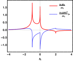
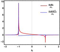
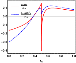
Figure 7: Average and the variance of the statistics of work done : (a)  Three spin interaction Ising model (b)  XY spin chain model, and (c)  SSH model.

The integral in the expression for the work done is difficult to evaluate analytically in the three spin and XY model case, but the integral in the variance can be solved by using contour integration. For simplicity, here we present the results for the SSH model only. The work done on the SSH model can be expressed as

$$\left\langle W\right\rangle=\frac{-1}{2\pi}\int_{0}^{\pi}R_{f}(\cos\phi_{f}\cos\phi_{i}+\sin\phi_{f}\sin\phi_{i})dk~{}.$$ (62)

This integral can be performed analytically, and the final expression can be written in terms of the elliptic functions as

$$\left\langle W\right\rangle=\frac{-1}{2\pi}\frac{1}{t_{1i}t_{2i}}\Bigg{[}(t_{1i}+t_{2i})(t_{1i}t_{2f}+t_{1f}t_{2i})\textit{F}_{1}\Big{[}\frac{4t_{1i}t_{2i}}{(t_{1i}+t_{2i})^{2}}\Big{]}-(t_{1i}-t_{2i})(t_{1i}t_{2f}-t_{1f}t_{2i})\textit{F}_{2}\Big{[}\frac{4t_{1i}t_{2i}}{(t_{1i}+t_{2i})^{2}}\Big{]}~{}.\Bigg{]}$$ (63)

where $F_{1}$ and $F_{2}$ are elliptic integrals. Note that the above expression is valid only away from the critical point since Eq. (63) is not defined at ($t_{1i}=t_{2i}$).

Similarly, the variance of the work done can be expressed as

$$\left\langle(\Delta W)^{2}\right\rangle=\begin{cases}\frac{(t_{1i}t_{2f}-t_{1f}t_{2i})^{2}}{4t^{2}_{2i}}&\text{$|t_{2i}|>|t_{1i}|$\quad Topological phase}\\ \frac{(t_{1i}t_{2f}-t_{1f}t_{2i})^{2}}{4t^{2}_{1i}},&\text{$|t_{2i}|<|t_{1i}|$\quad Non Topological Phase}\\ \end{cases}$$ (64)

The above equation is continuous at $t_{1i}=t_{2i}$, but its derivative reflects non-analytical behaviour around the critical point.

We plot the derivative of work done and its variance in Fig. 7 for three different free fermionic models considered. These quantities exhibit a non-analytical nature close to the critical points of the examined models. At $h=\pm 1$ for the XY model, at $h=J_{3}\pm 1$, $h=-J_{3}$ for the three spin interaction model, and at $t_{1}=t_{2}$ for the SSH model, it shows non-analyticity. Parameters used in these plots are, Fig. 7: $J_{3f}=0.5$, $J_{3i}=1$, $h_{f}=1$, Fig. 7: $\gamma_{f}=0.5$, $\gamma_{i}=0.1$, $h_{f}=0.6$, and Fig. 7: $t_{2f}=0.8$, $t_{2i}=0.5$, $t_{1f}=0.6.$

VI Conclusions and discussions

Our first motivation behind this paper was to see the qualitative difference in SC by considering three different types of interactions in spin chain models, the first with a two-spin interaction term, the second with a three-spin interaction term, and the third with dimerized interaction (SSH model). Because all three models are free fermion models, the evolution of SC is almost the same in each scenario.

The second motivation was to study SC as a probe to examine the quantum and topological phase transitions. In essence, we have found that the derivative of the SC has a non-analytical behaviour at the critical point for all three models. We study the problem under single and multiple (Sudden) quenches, where there is no sign of discontinuity near the critical point. Still, they attain steady state value for a long time, as mentioned in captua . We found that complexity reaches a steady state value earlier when the the final value of the parameter is close to a critical point than when the parameter’s initial value is at critical points; this behaviour applies to both single and multiple quench scenarios. In the time-dependent oscillating parameter case, when we plot the complexity with respect to the parameter (in the case of three spin and XY spin, it is $h_{c}$, while for SSH, it is $t_{1}$, $t_{2}$), there are peaks at the critical value of the parameter. On the other hand, when we examine the complexity with respect to a number of oscillations, first, it reaches the maximum value. Then it oscillates around an average value without any sign of discontinuity at the critical point.

Furthermore, we have also calculated the statistics of the work done under quench and explained their relationship with the Lanczos coefficients. The derivative of average work done and variance with respect to the parameter displayed non-analytical behaviour around critical points in all three models.

In this paper, we have confined our attention to the cases where the model can be mapped to a free-fermion model, which in turn made an analytical approach possible. It will be interesting to study the dynamics of SC in the more generic model, where this kind of mapping is not possible, which we left for future work.

VII Acknowledgements

We thank Prof. Tapobrata Sarkar, Kunal Pal and Kuntal Pal for their guidance and discussions. We are also thankful to Pritam Banerjee for his help and suggestions. We appreciate Pratik Nandy and Jacques H.H. Perk’s concern and important suggestions.

Appendix A Details of three spin interaction Ising model

For three spin case in Eq. (8), in JW transformation, Pauli matrices can be written in terms of the Fermionic operator as

$$c_{i}=\sigma^{-}_{i}\exp\Big{(}-i\pi\sum_{j=1}^{i-1}\sigma^{+}_{j}\sigma^{-}_{j}\Big{)}~{},~{}~{}\sigma^{z}_{i}=2c^{\dagger}_{i}c_{i}-1~{},$$ (65)

where $\sigma^{+}=(\sigma^{x}+i\sigma^{y})/2$, $\sigma^{-}=(\sigma^{x}-i\sigma^{y})/2$, and they satisfy the following standard anticommutation relations

$$[c^{\dagger}_{i}c_{j}]_{+}=\delta_{ij},~{}~{}\text{and}~{}~{}[c^{\dagger}_{i},c^{\dagger}_{j}]_{+}=[c_{i},c_{j}]_{+}=0~{}.$$

Now using the Fourier transformation mentioned in the main text, we can write the Hamiltonian as

$$H=-\sum_{k>0}(h+\cos{k}-J_{3}\cos{2k})(c^{\dagger}_{k}c_{k}+c^{\dagger}_{-k}c_{-k})+i(\sin{k}-J_{3}\sin{2k})(c^{\dagger}_{k}c^{\dagger}_{-k}+c_{k}c_{-k})~{}.$$ (66)

This can be rewritten in the following form

$$H=-\sum_{k}\Big{[}\mathbf{I}(h+\cos{k}-J_{3}\cos{2k})+\mathbf{\Phi}_{k}^{\dagger}\vec{R}(k).\vec{\sigma}\mathbf{\Phi}_{k}\Big{]}~{},$$ (67)

where $\mathbf{I}$ is identity matrix, $\mathbf{\Phi}_{k}=\begin{bmatrix}c_{k}\\ c_{-k}^{\dagger}\\ \end{bmatrix}$, $\vec{R}=\begin{bmatrix}0\\ J_{3}\sin 2k-\sin k\\ h+\cos k-J_{3}\cos 2k\\ \end{bmatrix}$, and $\vec{\sigma}$ = $(\sigma_{x},\sigma_{y},\sigma_{z})$. Here we consider periodic boundary conditions, so that $k=\frac{2n\pi}{L}$, where $n=,1,2,3\cdots\frac{N}{2}$, assuming $N$ is even. Furthermore, we can diagonalize the above Hamiltonian by using a Bogoliubov transformation of the form

$$\eta_{k}=-\cos{(\frac{\phi}{2})}c^{\dagger}_{-k}+i\sin{(\frac{\phi}{2})}c_{k}$$ (68)

$$\eta^{\dagger}_{-k}=i\cos{(\frac{\phi}{2})}c_{k}+\sin{(\frac{\phi}{2})}c^{\dagger}_{-k}~{},$$ (69)

where we have defined

$$\cos{\phi}=\frac{R_{3}}{R};\qquad R_{3}=h+\cos{k}-J_{3}\cos{2k}~{},\qquad R_{2}=J_{3}\sin{2k}-\sin{k}~{},\qquad R=\sqrt{R_{2}^{2}+R_{3}^{2}}=|\vec{R}(k)|~{}.$$

The diagonal form of the Hamiltonian can be written as

$$H=\sum_{k>0}R(k)[-\eta_{-k}\eta_{-k}^{\dagger}+\eta_{k}^{\dagger}\eta_{k}]~{}.$$ (70)

The ground state is defined by the condition $\eta_{k}\ket{\psi_{gs}}=0$ can be written as

$$\ket{\psi_{gs}}=\prod_{k>0}\sin{(\frac{\phi}{2})}\ket{0,0}-i\cos{(\frac{\phi}{2})}\ket{1,1}$$ (71)

Now we describe how the above Hamiltonian can be written as an element of the $su(2)$ algebra. $su(2)$ algebra is defined by the following commutation relations

$$[J_{z},J_{\pm}]=\pm J_{\pm},\quad[J_{+},J_{-}]=2J_{z},\quad[J_{\pm},I]=0,\quad[J_{z},I]=0~{}.$$

We have to find out the operator in our problem which satisfies the above relations; then we represent them by $J_{z}$, $J_{+}$, $J_{-}$. To this end, we first define

$$J^{k}_{0}=\frac{1}{2}(c^{\dagger}_{k}c_{k}-c_{-k}c^{\dagger}_{-k})~{},~{}J^{k}_{+}=c^{\dagger}_{k}c^{\dagger}_{-k}~{},~{}~{}J^{k}_{-}=c_{-k}c_{k}~{},$$ (72)

so that the form of the above Hamiltonian in terms of these operators can be written as

$$H=\sum_{k>0}R_{1}I^{k}+R_{1}J_{z}^{+k}+\frac{i}{2}R_{2}J_{+}^{+k}-\frac{i}{2}R_{2}(J_{-}^{+k})~{},$$

here $R_{1}$, and $R_{2}$ can be replaced by $R\cos{\phi}$, $R\sin{\phi}$, respectively, where $R=\sqrt{R_{1}^{2}+R_{2}^{2}}$.

Appendix B Details of the XY spin chain

In this appendix, we show that the Hamiltonian of the XY spin chain can be written as an element of the $su(2)$ Lie algebra and obtain the ground state of the model. The relation between the $su(2)$ generators and the creation and annihilation operators are the same as those in Eq. (72). Using these the Hamiltonian in Eq. (31) can be rewritten as

$$H=\sum_{k>0}\Big{[}-2(h+\cos{k})J^{k}_{0}+i\gamma\sin{k}J^{k}_{+}-i\gamma\sin{k}J^{k}_{-}\Big{]}=\sum_{k>0}\Big{[}-2(R\cos\phi)J^{k}_{0}+iR\sin\phi J^{k}_{+}-iR\sin\phi J^{k}_{-}\Big{]}~{},$$ (73)

where we have defined $R(k)=\sqrt{R_{2}^{2}+R_{3}^{2}}$, with $R_{2}=\gamma\sin{k}$, $R_{3}=h+\cos{k}$, $\phi=\tan^{-1}\frac{|R_{2}|}{R_{3}}$. By using the Bogoliubov transformations of the form written in Eq. (68), with $\phi=\cos^{-1}\Big{[}\frac{h+\cos k}{\gamma\sin k}\Big{]}$ we diagonalize the Hamiltonian of Eq. (73), so that the final form of the Hamiltonian is

$$H=\sum_{k>0}R(k)\Big{[}\eta^{\dagger}_{k}\eta_{k}+\eta^{\dagger}_{-k}\eta_{-k}-1\Big{]}~{}.$$ (74)

The form for the ground state is defined by the condition $\eta_{k}\ket{\psi_{g}}=0$ is the same as in Eq. (71), and it can be written as a $SU(2)$ coherent state of the form

$$\ket{\psi_{g}}=\prod_{k>0}\sin\frac{\phi_{i}}{2}e^{-i\cot\frac{\phi_{i}}{2}J_{+}^{k}}\ket{\frac{1}{2},\frac{-1}{2}}_{k}~{}.$$ (75)

Appendix C Duality Transformation

This section will explore the relationship between the XY-spin chain model and the three-spin interaction TIM under the duality transformation. For details, see jjh ; jjh1 .

$$A_{n}=\sum_{j=1}^{N}\sigma^{x}_{j}\left(\prod^{j+n-1}_{k=j+1}\sigma^{z}_{k}\right)\sigma^{x}_{j+n}$$

$$A_{-n}=\sum_{j=1}^{N}\sigma^{y}_{j}\left(\prod^{j+n-1}_{k=j+1}\sigma^{z}_{k}\right)\sigma^{y}_{j+n}$$

$$A_{0}=-\sum_{j=1}^{N}\sigma^{z}_{j},\quad A_{1}=\sum_{j=1}^{N}\sigma^{x}_{j}\sigma^{x}_{j+1}\quad A_{-1}=\sum_{j=1}^{N}\sigma^{y}_{j}\sigma^{y}_{j+1}\quad A_{2}=\sum_{j=1}^{N}\sigma^{x}_{j}\sigma^{z}_{j+1}\sigma^{x}_{j+2}$$

$$\tau^{z}_{n}=\sigma^{x}_{n-1}\sigma^{x}_{n},\quad\tau^{x}_{n}=\prod^{n-1}_{k=1}\sigma^{z}_{k}$$

where $\tau^{\alpha}_{n}$ dual quantum spins, satisfying Pauli spin algebra located at the centres of the bonds of the original lattice

$$\mathcal{H}=-\frac{1}{2}\Big{(}\sum_{i}\sigma^{z}_{i}\Big{[}h+J_{3}\sigma^{x}_{i-1}\sigma^{x}_{i+1}\Big{]}+J_{x}\sum_{i}\sigma^{x}_{i}\sigma^{x}_{i+1}\Big{)}$$ (76)

Above Hamiltonian consist of $A_{0}$ , $A_{1}$ and $A_{2}$, where as XY-spin chain Hamiltonian Eq.(30) consist of $A_{0}$ , $A_{1}$ , $A_{-1}$. By using dual representation, the Hamiltonian Eq.(76) can be written in XY spin chain form

$$\mathcal{H}=-\frac{1}{2}\Big{(}\sum_{n}h\tau^{x}_{n}\tau^{x}_{n+1}-J_{3}\tau^{y}_{n}\tau^{y}_{n+1}+J_{x}\sum_{n}\tau^{z}_{n}\Big{)}$$ (77)

XY-spin chain model in general form

$$H=-\sum_{i}\big{[}J^{\prime}_{x}\sigma^{x}_{i}\sigma^{x}_{i+1}+J_{y}\sigma^{y}_{i}\sigma^{y}_{i+1}+h^{\prime}\sigma^{z}_{i}]$$ (78)

Eq.(76) can map into Eq.(78) with $\frac{h^{\prime}}{J^{\prime}_{x}-J_{y}}=\frac{J_{x}}{h+J_{3}}$ and $\frac{h^{\prime}}{J^{\prime}_{x}+J_{y}}=\frac{J_{x}}{h-J_{3}}$

Appendix D Auxillary Equation for time-dependent case

In this appendix, we will find out the relation of $\gamma(t)$ and $\beta(t)$ defined in Eq. (24). For details, see Refs. lai ; Maam . Comparing Eqs. (11), (33), and (41), we find out that the Hamiltonian in our problem has the following form (with $\phi(t)=\frac{\pi}{2}$)

$$H=f(t)J_{0}^{k}+g(t)[J_{+}^{k}e^{i\phi(t)}+J_{-}^{k}e^{-i\phi(t)}]~{}.$$

where $f(t)$, $g(t)$, and $\phi(t)$ are real functions of time. The Schrodinger equation governs the time evolution of the quantum state.

$$i\frac{d}{dt}\ket{\psi(t)}=H(t)\ket{\psi(t)}~{}.$$

Next, we define the invariant operator $\mathcal{I}(t)$, which satisfies the following conditions

$$\frac{d\mathcal{I}}{dt}\equiv i\frac{\partial\mathcal{I}}{\partial t}+[\mathcal{I},H]=0~{},~{}~{}\text{and}~{}~{}\mathcal{I}^{\dagger}=\mathcal{I}~{}.$$ (79)

Using the above conditions for the invariant operator, we see that it satisfies the equation.

$$i\frac{d}{dt}(\mathcal{I}\ket{\psi(t)})=H(t)(\mathcal{I}\ket{\psi(t)})~{}.$$

Therefore if $\ket{\psi(t)}$ satisfy Schrodinger equation so does $\mathcal{I}\ket{\psi(t)}$. For our purposes, we define the invariant operator as

$$\mathcal{I}(t)=\hat{R}(t)\hat{J_{0}}\hat{R}^{\dagger}(t)~{},$$ (80)

where

$$\hat{R}(t)=\exp\Big{[}\frac{\gamma(t)}{2}\Big{(}\hat{J}_{+}e^{-i\beta(t)}-\hat{J}_{-}e^{i\beta(t)}\Big{)}\Big{]}~{}.$$ (81)

Time-dependent parameter $\gamma(t)$ and $\beta(t)$ are related to the functions $f(t)$ and $g(t)$ appearing in the Hamiltonian through

$$\dot{\gamma}=2g(t)\sin{(\phi+\beta)}~{},\qquad\big{(}\dot{\beta}-f(t)\big{)}\sin{\gamma}=2g(t)\cos{\gamma}\cos{(\phi+\beta)}~{}.$$ (82)

We can derive the above equations by using Eqs. (79), (81), and (80) and the following relations

$$\hat{R}^{\dagger}(t)\hat{J}_{+}\hat{R}(t)=\hat{J}_{+}\cos^{2}\frac{\gamma}{2}-\hat{J}_{-}e^{2i\beta}\sin^{2}\frac{\gamma}{2}-\hat{J}_{0}e^{i\beta}\sin\gamma~{},$$

$$\hat{R}^{\dagger}(t)\hat{J}_{-}\hat{R}(t)=\hat{J}_{-}\cos^{2}\frac{\gamma}{2}-\hat{J}_{+}e^{-2i\beta}\sin^{2}\frac{\gamma}{2}-\hat{J}_{0}e^{-i\beta}\sin\gamma~{},$$

$$\hat{R}^{\dagger}(t)\hat{J}_{0}\hat{R}(t)=\hat{J}_{0}\cos\gamma+\frac{1}{2}(\hat{J}_{+}e^{-i\beta}+\hat{J}_{-}e^{i\beta})\sin\gamma~{},$$

as well as

$$\hat{R}^{\dagger}(t)\Big{[}i\frac{\partial\hat{R}(t)}{\partial t}\Big{]}=-2\hat{J}_{0}\dot{\beta}\sin^{2}\frac{\gamma}{2}+\hat{J}_{+}e^{-i\beta}\Big{(}i\frac{\dot{\gamma}}{2}+\frac{\dot{\beta}}{2}\sin\gamma\Big{)}+{J}_{-}e^{i\beta}\Big{(}-i\frac{\dot{\gamma}}{2}+\frac{\dot{\beta}}{2}\sin\gamma\Big{)}~{},$$

To solve the differentiation of an operator by a parameter, we use the relation given below (where $\lambda$ represents the parameter on which operator $A$ depends)

$$\frac{\partial\exp{\hat{A}}}{\partial\lambda}=\int_{0}^{1}ds\exp{(1-s)\hat{A}}\frac{\partial{\hat{A}}}{\partial\lambda}\exp{s\hat{A}}~{}.$$

Since $\phi=\frac{\pi}{2}$ and by symmetry, we choose $\beta=-\phi$. This led to the following equations.

$$\dot{\gamma}\approx 0~{}~{}\text{and}~{}~{}-f(t)\sin{\gamma}=2g(t)\cos{\gamma}~{}.$$

From the second equation, we obtain

$$\gamma(t)=\tan^{-1}\Big{[}-\frac{2g(t)}{f(t)}\Big{]}~{}.$$

To satisfy the condition $\dot{\gamma}(t)\approx 0$ we have to take $\omega\approx\textit{small}$ (adiabatic approximation, the variation in $\gamma(t)$ is negligible).

Appendix E Time Dependent state under periodic variation of parameter

In this section, we find the explicit expression of time evolved state under periodic variation of parameters. Let $\ket{n}$ be the eigenstate of $J_{0}$ with eigenvalue $j$

$$J_{0}\ket{n}=j\ket{n}$$

Eigenstate of $\mathcal{I}(t)$

$$\mathcal{I}(t)\ket{n,t}=j\ket{n,t}\qquad\ket{n,t}=\hat{R}(t)\ket{n}$$

According to the LR theory Lewis the eigenvectors of $\mathcal{I}(t)$ are related to the general state by time-dependent gauge transformation

$$\ket{\psi(t)}=\sum_{n}c_{n}e^{i\alpha_{n}(t)}\ket{n,t}~{},$$

where $c_{n}$ are time-independent coefficients, and the time-dependent phase factor $\alpha_{n}(t)$ can be written as

$$\alpha_{n}(t)=\int_{0}^{t}dt^{\prime}\bra{n,t^{\prime}}i\frac{\partial}{\partial t^{\prime}}-\hat{H}(t^{\prime})\ket{n,t^{\prime}}=\int_{0}^{t}dt^{\prime}\bra{n}[\hat{R}^{\dagger}(t^{\prime})i\frac{\partial}{\partial t^{\prime}}\hat{R}(t^{\prime})-\hat{R}^{\dagger}(t^{\prime})\hat{H}(t^{\prime})\hat{R}(t^{\prime})]\ket{n}~{}.$$ (83)

which can be simplified to:

$$\alpha_{n}(t)=-j\int_{0}^{t}dt^{\prime}\Big{[}f(t^{\prime})+2(\dot{\beta}-f(t))\sin^{2}{\frac{\gamma}{2}}-2g(t)\sin{\gamma}\cos{(\phi+\beta)}\Big{]}$$

and

$$\epsilon(t)=\int_{0}^{t}dt^{\prime}[f(t^{\prime})+2(\dot{\beta}-f(t))\sin^{2}{\frac{\gamma}{2}}-2g(t)\sin{\gamma}\cos{(\phi+\beta)}]~{}.$$

At $t=0$, we have $\ket{\psi(0)}=\hat{R}(0)\sum_{n}c_{n}\ket{n}$. In our case, we take $\ket{\psi(0)}$ as the ground state of the initial Hamiltonian, i.e. the one given in Eq. (23). Now by using the BCH formula, we obtain

$$\hat{R}^{\dagger}(0)=\exp(z_{0}J_{+})\exp(\log(1+z_{0}\bar{z}_{0})J_{0})\exp(-\bar{z_{0}}J_{-})~{},~{}~{}\text{with}~{}~{}z_{0}=-i\tan(\frac{\gamma(0)}{2})~{},~{}~{}\text{and}~{}~{}$$

$$\hat{R}(t)=\exp(z_{t}J_{+})\exp(\log(1+z_{t}\bar{z}_{t})J_{0})\exp(-\bar{z_{t}}J_{-})~{},~{}~{}\text{with}~{}~{}z_{t}=i\tan(\frac{\gamma(t)}{2})~{},~{}~{}\text{and}~{}~{}$$

$$\hat{R}_{i}=\exp(z_{i}J_{+})\exp(\log(1+z_{i}\bar{z}_{i})J_{0})\exp(-\bar{z_{i}}J_{-})~{},~{}~{}\text{with}~{}~{}z_{i}=-i\cot(\frac{\phi_{i}}{2})~{}.$$

$$\begin{split}\ket{\psi(t)}=\prod_{k>0}\cos^{2j}{\frac{\gamma(0)}{2}}\sin^{2j}(\frac{\phi_{i}}{2})\cos^{2j}{\frac{\gamma(t)}{2}}e^{-ij\epsilon(t)}(1+z_{i}z_{0})^{2j}(1+z_{t}\alpha e^{-i\epsilon(t)})^{2j}\\ \exp\Big{[}[z_{t}+\frac{\alpha\sec^{2}{\frac{\gamma(t)}{2}}e^{-i\epsilon(t)}}{1+\alpha z_{t}e^{-i\epsilon(t)}}]J_{+}^{k}]\Big{]}\ket{j,-j}_{k}\end{split}$$ (84)

where $\alpha=z_{0}+\frac{z_{i}\sec^{2}[\frac{\gamma(0)}{2}]}{1+z_{i}z_{0}}$. The return amplitude here can be written as

$$\mathcal{S}(t)=\sum_{n=0}^{2j}(-z_{i})^{n}\frac{(2j)!}{(2j-n)!n!}\Big{[}z_{t}+\frac{\alpha\sec^{2}{\frac{\gamma(t)}{2}}e^{-i\epsilon(t)}}{1+\alpha z_{t}e^{-i\epsilon(t)}}\Big{]}^{n}A(t)~{},$$

where

$$A(t)=\cos^{2j}\Big{[}{\frac{\gamma(0)}{2}}\Big{]}\sin^{4j}\Big{[}{\frac{\phi_{i}}{2}}\Big{]}\cos^{2j}\Big{[}{\frac{\gamma(t)}{2}}\Big{]}e^{-ij\epsilon(t)}\big{(}1+z_{i}z_{0}\big{)}^{2j}\big{(}1+z_{t}\alpha e^{-i\epsilon(t)}\big{)}^{2j}~{}.$$

When $j=\frac{1}{2}$, we get back the expression for the return amplitude provided in Eq. (27).

For periodic condition $\gamma(nT)=\gamma(0)=\gamma$

$$\begin{split}\ket{\psi(nT)}=\prod_{k>0}\Big{[}[\cos(\frac{\epsilon(nT)}{2})\sin(\frac{\phi_{i}}{2})-i\sin(\frac{\epsilon(nT)}{2})\sin(\gamma-\frac{\phi_{i}}{2})]\ket{\frac{1}{2},\frac{-1}{2}}_{k}+\\ [-\cos(\gamma-\frac{\phi_{i}}{2})\sin(\frac{\epsilon(nT)}{2})-i\cos(\frac{\epsilon(nT)}{2})\cos(\frac{\phi_{i}}{2})]\ket{\frac{1}{2},\frac{1}{2}}_{k}\Big{]}~{}.\end{split}$$ (85)

References

- (1) S. Sachdev, Quantum Phase Transitions, 2nd ed. (Cambridge University Press, Cambridge, 2011).
- (2) S. Chapman and G. Policastro, “Quantum computational complexity from quantum information to black holes and back,” Eur. Phys. J. C 82 (2022) no.2, 128.
- (3) Jefferson, R. A., & Myers, R. C., Circuit complexity in quantum field theory, Journal of High Energy Physics, 2017, 107 (2017).
- (4) Khan, R., Krishnan, C., & Sharma, S., Circuit complexity in fermionic field theory, Physical Review D, 98, 126001 (2018).
- (5) A. Bhattacharyya, A. Shekar and A. Sinha, “Circuit complexity in interacting QFTs and RG flows,” JHEP 10 (2018), 140.
- (6) Liu, F., Whitsitt, S., Curtis, J. B., Lundgren, R., Titum, P., Yang, Z.-C., Garrison, J. R., & Gorshkov, A. V., Circuit complexity across a topological phase transition, Physical Review Research, 2, 013323 (2020).
- (7) N. Jaiswal, M. Gautam and T. Sarkar, “Complexity and information geometry in the transverse XY model,” Phys. Rev. E 104 (2021) no.2, 024127.
- (8) Gautam, M., Jaiswal, N., Gill, A., & Sarkar, T. (2022), arXiv e-prints, arXiv:2207.14090.
- (9) Balasubramanian, V., Caputa, P., Magan, J. M., & Wu, Q., Quantum chaos and the complexity of spread of states, Physical Review D, 106, 046007 (2022).
- (10) V. S. Viswanath, G. Müller, The Recursion Method Application to Many-Body Dynamics, Springer (1994).
- (11) Lanczos, Cornelius. “An iteration method for the solution of the eigenvalue problem of linear differential and integral operators.” Journal of Research of the National Bureau of Standards 45 (1950): 255-282.
- (12) Parker, D. E., Cao, X., Avdoshkin, A., Scaffidi, T., & Altman, E., Physical Review X, 9, 041017 (2019).
- (13) Adhikari, K., Choudhury, S., & Roy, A. ,Krylov Complexity in Quantum Field Theory, arXiv e-prints, arXiv:2204.02250 (2022).
- (14) Adhikari, K., & Choudhury, S., Cosmological Krylov Complexity, Fortschritte der Physik, 70, 2200126 (2022).
- (15) Bhattacharjee, B., Sur, S., & Nandy, P., Probing quantum scars and weak ergodicity breaking through quantum complexity, Physical Review B, 106, 205150 (2022).
- (16) Caputa, P., & Liu, S., Quantum complexity and topological phases of matter, Physical Review B, 106, 195125 (2022).
- (17) Caputa, P., Magan, J. M., & Patramanis, D., Geometry of Krylov complexity, Physical Review Research, 4, 013041 (2022).
- (18) Caputa, P., Gupta, N., Haque, S. S., Liu, S., Murugan, J., & Van Zyl, H. J. R., Spread complexity and topological transitions in the Kitaev chain, Journal of High Energy Physics, 2023, 120 (2023).
- (19) Rabinovici, E., Sánchez-Garrido, A., Shir, R., & Sonner, J., Journal of High Energy Physics, 2022, 151 (2022).
- (20) A. A. Nizami and A. W. Shrestha, “Krylov construction and complexity for driven quantum systems,” [arXiv:2305.00256 [quant-ph]].
- (21) Quan, H. T., Song, Z., Liu, X. F., Zanardi, P., & Sun, C. P. Physical Review Letters, 96, 140604 (2006).
- (22) Campos Venuti, L., & Zanardi, P., Physical Review A, 81, 022113 (2010).
- (23) Polkovnikov, A., Sengupta, K., Silva, A., & Vengalattore, M. Reviews of Modern Physics, 83, 863 (2011).
- (24) Johannesson, H., & Jafari, R., Decoherence from Spin Environments: Loschmidt Echo and Quasiparticle Excitations, APS March Meeting Abstracts, 2018, K44.005 (2018).
- (25) Jafari, R., & Johannesson, H., Loschmidt Echo Revivals: Critical and Noncritical, Physical Review Letters, 118, 015701 (2017).
- (26) Jafari, R., Johannesson, H., Langari, A., & Martin-Delgado, M. A., Quench dynamics and zero-energy modes: The case of the Creutz model, Physical Review B, 99, 054302 (2019).
- (27) Kopp, A., & Chakravarty, S., Criticality in correlated quantum matter, APS March Meeting Abstracts, N45.002 (2006).
- (28) Divakaran, U., & Dutta, A., The effect of the three-spin interaction and the next-nearest neighbour interaction on the quenching dynamics of a transverse Ising model, arXiv e-prints, arXiv:0801.2621 (2008).
- (29) Lieb, E., Schultz, T., & Mattis, D., Two soluble models of an antiferromagnetic chain, Annals of Physics, 16, 407 (1961).
- (30) Pfeuty, P., The one-dimensional Ising model with a transverse field, Annals of Physics, 57, 79 (1970).
- (31) Kogut, J. B., An introduction to lattice gauge theory and spin systems, Reviews of Modern Physics, 51, 659 (1979).
- (32) Perelomov, A. M., Generalized coherent states and their applications, Moscow Izdatel Nauka (1987).
- (33) Russomanno, A., Silva, A., & Santoro, G. E., Periodic Steady Regime and Interference in a Periodically Driven Quantum System, Physical Review Letters, 109, 257201 (2012).
- (34) Mukherjee, V., & Dutta, A., Effects of interference in the dynamics of a spin- 1/2 transverse XY chain driven periodically through quantum critical points, Journal of Statistical Mechanics: Theory and Experiment, 2009, 05005 (2009).
- (35) Sharma, S., Russomanno, A., Santoro, G. E., & Dutta, A., Loschmidt echo and dynamical fidelity in periodically driven quantum systems, EPL (Europhysics Letters), 106, 67003 (2014).
- (36) Lai, Y.-Z., Liang, J.-Q., Müller-Kirsten, H. J. W., & Zhou, J.-G., Time-dependent quantum systems and the invariant Hermitian operator, Physical Review A, 53, 3691 (1996).
- (37) Maamache, M., Unitary transformation approach to the cyclic evolution of SU(1, 1) and SU(2) time-dependent systems and geometrical phases, Journal of Physics A Mathematical General, 31, 6849 (1998).
- (38) Lewis, H. R., & Riesenfeld, W. B., An Exact Quantum Theory of the Time-Dependent Harmonic Oscillator and of a Charged Particle in a Time-Dependent Electromagnetic Field, Journal of Mathematical Physics, 10, 1458 (1969).
- (39) Sharma, S., Mukherjee, V., & Dutta, A., Study of Loschmidt Echo for a qubit coupled to an XY-spin chain environment, European Physical Journal B, 85, 143 (2012).
- (40) Zhang, Z.-Z., & Wu, W., Physical Review E, 106, 034104 (2022).
- (41) Zhou, Z.-Y., Xiang, Z.-L., You, J. Q., & Nori, F. Physical Review E, 104, 034107 (2021),.
- (42) Talkner, P., Lutz, E., & Hänggi, P. Fluctuation theorems: Work is not observable. Phys. Rev. E 75, 050102(R) (2007)
- (43) Kurchan, J. (2000), arXiv e-prints, cond-mat/0007360.
- (44) Jarzynski, C., Physical Review Letters, 78, 2690 (1997).
- (45) Silva, Alessandro, Statistics of the Work Done on a Quantum Critical System by Quenching a Control Parameter,101,120603 (2008)
- (46) Sotiriadis, Spyros, Gambassi, Andrea, and Silva, Alessandro, Statistics of the work done by splitting a one-dimensional quasicondensate, 87,052129 (2013).
- (47) Perk, J. H. H., Onsager algebra and cluster XY-models in a transverse magnetic field, arXiv e-prints, arXiv:1710.03384 (2017).
- (48) Perk, J. H. H., Quadratic identities for Ising model correlations, Physics Letters A, 79, 3 (1980).