What part of a numerical problem is ill-conditioned?

Abstract.

Many numerical problems with input ${x}$ and output ${y}$ can be formulated as an system of equations $F({x},{y})=0$ where the goal is to solve for ${y}$. The condition number measures the change of ${y}$ for small perturbations to ${x}$. From this numerical problem, one can derive a (typically underdetermined) subproblem by omitting any number of constraints from $F$. We propose a condition number for underdetermined systems that relates the condition number of a numerical problem to those of its subproblems. We illustrate the use of our technique by computing the condition of two problems that do not have a finite condition number in the classic sense: any two-factor matrix decompositions and Tucker decompositions.

1. Introduction

Many numerical problems can be modelled as a system of equations $F({x},{y})=c$, where $F:{\mathcal{X}}\times{\mathcal{Y}}\to\mathcal{Z}$ is a smooth map between smooth manifolds, $c$ is a constant (often $c=0$), ${x}$ is the input, and ${y}$ is an output or solution. For a given input ${x}$, the goal is to find a solution of $F({x},{y})=c$. The condition number (defined below) is a common indicator of the numerical difficulty of the system, as it measures the sensitivity of a solution ${y}$ with respect to the input ${x}$ [5].

Suppose we have two systems $R({x},{y})=c$ with $R:{\mathcal{X}}\times{\mathcal{Y}}\to\mathcal{Z}$ and $S({x},{y})=c^{\prime}$ with $S:{\mathcal{X}}\times\widetilde{{\mathcal{Y}}}\to\widetilde{\mathcal{Z}}$ and ${\mathcal{Y}}\subseteq\widetilde{{\mathcal{Y}}}$. Then we call the latter a subproblem of the former if every pair $({x},{y})$ that solves $R({x},{y})=c$ satisfies $S({x},{y})=c^{\prime}$. We also call $R({x},{y})=c$ a refinement of $S({x},{y})=c^{\prime}$ in this case. That is, the subproblem accepts at least as many solutions as the refinement. In particular, either system may be underdetermined, i.e., the input may not determine a unique or even finite number of solutions. For example, consider the following common numerical problems and corresponding subproblems.

• If $R({x},{y})=c$ is a system of $n$ equations, any subset of those equations defines a subproblem.

• A rank-revealing QR-decomposition of a matrix ${X}\in\mathbb{R}^{m\times n}$ of rank $k$ is a tuple ${Y}=(Q,R)\in\mathbb{R}^{m\times k}\times\mathbb{R}^{k\times n}$ such that ${X}=QR$, $R$ is upper-triangular, and the columns of $Q$ are orthonormal. Omitting the constraints on the structure of $Q$ and $R$ yields a subproblem, which we call a two-factor decomposition.

• For a matrix ${X}\in\mathbb{R}^{m\times n}$ of rank $k$ with distinct singular values, computing the left singular vectors corresponding to all nonzero singular values is a refinement of computing a basis for the image.

• A higher-order singular value decomposition [6] of a tensor ${\mathpzc{X}}\in\mathbb{R}^{n_{1}\times\dots\times n_{D}}$ of multilinear rank $(k_{1},\dots,k_{D})$ is a refined Tucker decomposition [24]. Similarly, computing a Tensor train decomposition is a subproblem of the TT-SVD problem [20].

In this paper, we introduce a condition number that formalises the following intuition: if it is difficult to solve a subproblem, then solving any refinement of it must be difficult as well. That is, the condition number of the subproblem is a lower bound for the condition number of the refinement. The framework we develop is useful for interpreting the condition of a numerical problem: a problem may be ill-conditioned because of an ill-conditioned subproblem or in spite of well-conditioned subproblems.

The key difficulty in providing such a framework is that the subproblem may be underdetermined, in which case it does not have a finite condition number in the classic sense. Thus, the standard condition number is rather crude, as it cannot tell apart well- and ill-conditioned underdetermined systems. We remedy this by introducing the least-squares condition number. Its relationship to the classic condition number is illustrated by fig. 1.1.

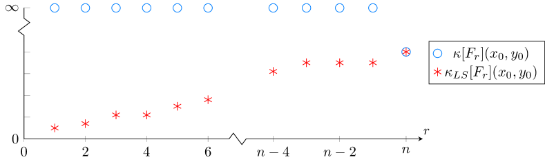
Figure 1.1. Condition of a hypothetical square system of independent polynomial equations. The system $f_{1}(x,y)=\dots=f_{n}(x,y)=0$ with $f_{i}:\mathbb{R}^{n}\times\mathbb{R}^{n}\to\mathbb{R}$ has an isolated solution $(x_{0},y_{0})$ and a finite condition number $\kappa$ at $(x_{0},y_{0})$. For $r\leq n$, the system $F_{r}(x,y):=(f_{1}(x,y),\dots,f_{r}(x,y))=0$ defines a subproblem. If $r<n$, the classic condition number $\kappa[F_{r}](x_{0},y_{0})$ of $F_{r}$ is infinite, but the newly proposed least-squares condition number $\kappa_{LS}[F_{r}](x_{0},y_{0})$ will provide a lower bound for $\kappa$.

Recall that, for a map $H:{\mathcal{X}}\to{\mathcal{Y}}$ between metric spaces and a point ${x}_{0}\in{\mathcal{X}}$, the condition number $\kappa[H]({x}_{0})$ is defined to be the smallest number $\kappa$ so that

(1.1) $$d_{{\mathcal{Y}}}(H({x}_{0}),H({x}))\leq\kappa\cdot d_{{\mathcal{X}}}({x}_{0},{x})+o(d_{{\mathcal{X}}}({x}_{0},{x}))\quad\text{as}\quad{x}\to{x}_{0},$$

where $d_{{\mathcal{X}}}$ and $d_{{\mathcal{Y}}}$ are the distances in ${\mathcal{X}}$ and ${\mathcal{Y}}$, respectively. The property that $\kappa[H]({x}_{0})$ is the smallest such number is called asymptotic sharpness. For a smooth map $H$ between Riemannian manifolds, Rice’s theorem [21] says that the condition number for the geodesic distance is $\kappa[H]({x}_{0})=\norm{DH({x}_{0})}$, where the linear map $DH({x}_{0}):T_{{x}_{0}}{\mathcal{X}}\to T_{H({x}_{0})}{\mathcal{Y}}$ is the differential of $H$ and $\norm{\cdot}$ is the spectral norm induced by the Riemannian metrics on ${\mathcal{X}}$ and ${\mathcal{Y}}$. In coordinates, $DH({x}_{0})$ is the Jacobian matrix.

For a determined system (i.e, one with finitely many solutions for every input), the sensitivity of the solutions can be studied as follows [5]. Let $({x}_{0},{y}_{0})$ be a particular solution satisfying $F({x}_{0},{y}_{0})=c$. Under general conditions described in [5], there exists a unique solution map, i.e., a smooth map $H_{{y}_{0}}:{x}\mapsto{y}$ defined on a neighbourhood of ${x}_{0}$ such that $H_{{y}_{0}}({x}_{0})={y}_{0}$ and $F({x},H_{{y}_{0}}({x}))=c$ for all ${x}$ close to ${x}_{0}$. Thus, the input ${x}$ corresponds to a locally unique solution ${y}=H_{{y}_{0}}({x})$ and $\kappa[H_{{y}_{0}}]({x})$ measures the sensitivity of this solution to small changes in the input ${x}$.

To define a condition number for underdetermined systems, we need some regularity assumptions. The following model is used throughout the article.

Definition 1.1.

Let ${\mathcal{X}},{\mathcal{Y}},\mathcal{Z}$ be smooth manifolds and let $c\in\mathcal{Z}$ be a constant. Let $F:{\mathcal{X}}\times{\mathcal{Y}}\rightarrow\mathcal{Z}$ be a smooth map. We call the equation $F({x},{y})=c$ a feasible constant-rank equation (FCRE) if the following holds:

1. for all ${x}\in{\mathcal{X}}$, there exists a point ${y}\in{\mathcal{Y}}$ such that $F({x},{y})=c$,

2. there exists a number $r\in\mathbb{N}$ so that $\rank\partialderivative{{y}}F({x}\,y)=r$ and $\rank DF({x},{y})=r$ for all ${x},{y}\in{\mathcal{X}}\times{\mathcal{Y}}$.

Note that if $r=\dim{\mathcal{Y}}=\dim\mathcal{Z}$, we obtain the usual hypothesis under which a unique solution map exists [5]. In this case, $\partialderivative{{y}}F({x},{y})$ is invertible. Note as well that if a map $F$ only satisfies this definition locally, the restriction of $F$ to a subset of its domain defines an FCRE.

Our first main theorem underlies the definition of the condition number of an FCRE.

Theorem 1.2.

Let $F({x},{y})=c$ be an FCRE as in Definition 1.1 and let $({x}_{0},{y}_{0})$ be any pair such that $F({x}_{0},{y}_{0})=c$. If $\mathcal{X}$ and $\mathcal{Y}$ are Riemannian manifolds, then there exist a neighbourhood $\widehat{{\mathcal{X}}}\subseteq{\mathcal{X}}$ of ${x}_{0}$ and a smooth map, called the least-squares solution map

$$H_{{y}_{0}}:\widehat{{\mathcal{X}}} \to{\mathcal{Y}}$$

$${x} \mapsto\arg\min_{\begin{subarray}{c}{y}\in{\mathcal{Y}}\\ F({x},{y})=c\end{subarray}}d_{{\mathcal{Y}}}({y}_{0},{y}),$$

where $d_{{\mathcal{Y}}}$ is the geodesic distance in ${\mathcal{Y}}$.

Figure 1.2. Simplified view of the solution sets and the least-squares solution map. For ${x}$ close to ${x}_{0}$, the point $H_{{y}_{0}}({x})$ is the projection of ${y}_{0}$ onto the solution set $\{{y}\mid F({x},{y})=c\}$.

That is, out of all possible solution maps, $H_{{y}_{0}}$ locally minimises the distance to ${y}_{0}$. Figure 1.2 shows a visualisation of $H_{{y}_{0}}$. The preceding theorem allows us to define our primary object of interest.

Definition 1.3.

In the context of Theorem 1.2, the least-squares condition number of $F$ at $({x}_{0},{y}_{0})$ is

$$\kappa_{LS}[F]({x}_{0},{y}_{0}):=\kappa[H_{{y}_{0}}]({x}_{0}).$$

Thus, $\kappa_{LS}$ expresses whether the equation $F({x},{y})=c$ has a solution close to ${y}_{0}$ if ${x}$ is a slight perturbation of ${x}_{0}$. If $d_{{\mathcal{X}}}$ and $d_{{\mathcal{Y}}}$ are the geodesic distances in ${\mathcal{X}}$ and ${\mathcal{Y}}$, respectively, we have the following asymptotically sharp error bound:

(1.2) $$\min_{\begin{subarray}{c}{y}\in{\mathcal{Y}},\\ F({x},{y})=c\end{subarray}}d_{{\mathcal{Y}}}({y}_{0},{y})\leq\kappa_{LS}[F]({x}_{0},{y}_{0})\cdot d_{{\mathcal{X}}}({x}_{0},{x})+o(d_{{\mathcal{X}}}({x}_{0},{x}))\,\,\text{as}\,\,{x}\to{x}_{0}.$$

Since this is a bound on the asymptotic behaviour as ${x}\to{x}_{0}$, the same bound holds for any distance $d$ such that $d({x}_{0},{x})=d_{{\mathcal{X}}}({x}_{0},{x})(1+o(1))$ as ${x}\to{x}_{0}$ and likewise for $d_{{\mathcal{Y}}}$.

Remark 1.4.

The classic condition number of equations on manifolds requires a unique solution map at the given solution pair $(x_{0},y_{0})$. If this map does not exist or is not unique, the condition number is either undefined [5] or infinite by definition [3]. If the classic condition number of an FCRE is finite, the unique solution map is the map from Theorem 1.2 and the condition number is the least-squares condition number.

The condition number of an underdetermined FCRE can be used as a lower bound for the condition number of any refinement of it. This is captured by the following statement, which follows by definition.

Corollary 1.5.

Consider the FCREs $R({x},{y})=c$ and $S({x},{y})=c^{\prime}$ such that the former is a refinement of the latter. If $R({x}_{0},{y}_{0})=c$ for some $({x}_{0},{y}_{0})$, then

$$\kappa_{LS}[S]({x}_{0},{y}_{0})\leq\kappa_{LS}[R]({x}_{0},{y}_{0}).$$

This statement can be used to examine what part of a numerical problem is difficult. That is, if a subproblem is ill-conditioned, this explains the ill-conditioning of the refinement. Alternatively, if $\kappa_{LS}[S]({x}_{0},{y}_{0})$ is small, then for $({x},{y})$ close to $({x}_{0},{y}_{0})$, the subproblem has a well-conditioned refinement with a unique solution. This refinement is given by the evaluation of $H_{{y}_{0}}$.

Our second main theorem provides an expression that is convenient for the numerical computation of the condition number, generalising [2, Equation (12.4)] and [5, Section 14.1.2].

Theorem 1.6.

If $F$ satisfies the assumptions of Theorem 1.2, then the least-squares condition number of $F$ is

$$\kappa_{LS}[F]({x}_{0},{y}_{0})=\norm{\left(\partialderivative{{y}}F({x}_{0},{y}_{0})\right)^{\dagger}\partialderivative{x}F({x}_{0},{y}_{0})},$$

where $\cdot^{\dagger}$ is the Moore–Penrose inverse and $\norm{\cdot}$ is the spectral norm.

An important class of systems of equations are equations of the form $G({y})-{x}=0$ for some smooth map $G:{\mathcal{Y}}\to\mathbb{R}^{m}$. In this case, Theorem 1.6 specialises to the following Riemannian generalisation of [7, Theorem C].

Corollary 1.7.

Let ${\mathcal{Y}}$ be a Riemannian manifold and let $G:{\mathcal{Y}}\to\mathbb{R}^{n}$ be a smooth map such that $\rank DG({y})$ is constant. Pick any point $({x}_{0},{y}_{0})$ on the graph of $G$. Then ${y}_{0}$ has a neighbourhood $\widehat{{\mathcal{Y}}}$ such that ${\mathcal{X}}:=G(\widehat{{\mathcal{Y}}})$ is an embedded submanifold of $\mathbb{R}^{n}$. Define

$$F:{\mathcal{X}}\times\widehat{{\mathcal{Y}}} \to\mathbb{R}^{n}$$

$$({x},{y}) \mapsto G({y})-{x}.$$

Then $F({x},{y})=0$ is an FCRE and $\kappa_{LS}[F]({x}_{0},{y}_{0})=\norm{DG({y}_{0})^{\dagger}}$.

For a map $G$ satisfying the assumptions in Corollary 1.7, we call the equation $G({y})-{x}=0$ a constant-rank inverse problem and we write $\kappa_{LS}^{inv}[G]({y}_{0}):=\kappa_{LS}[F]({x}_{0},{y}_{0})$. Note that $\norm{DG({y}_{0})^{\dagger}}$ is the reciprocal of the smallest nonzero singular value of $DG({y}_{0})$.

For specific systems, the expression for the condition number can be simplified further. For instance, consider the factorisation of a given matrix $X\in\mathbb{R}^{m\times n}$ of rank $k$ as $X=LR$, where $L\in\mathbb{R}^{m\times k}$, $R\in\mathbb{R}^{k\times n}$, and no structure is imposed on $L$ and $R$. The least-squares condition number of factorising $A$ into $L$ and $R$ is derived in section 4.

Proposition 1.8.

Let $G_{\mathcal{M}}(L,R):=LR$, where $L\in\mathbb{R}^{m\times k}$ and $R\in\mathbb{R}^{k\times n}$ have rank $k$. Let $\sigma_{i}(\cdot)$ denote the $i$th largest singular value of its argument, with the convention that $\sigma_{i}(L)=0$ for all $i>k$ and likewise for $R$. At every point $(L,R)$, we have

(1.3) $$\kappa_{LS}^{inv}[G_{\mathcal{M}}](L,R)=\frac{1}{\sqrt{\min\left\{\sigma_{k}(L)^{2}+\sigma_{n}(R)^{2},\;\sigma_{m}(L)^{2}+\sigma_{k}(R)^{2}\right\}}}$$

with respect to the Euclidean inner product on $\mathbb{R}^{m\times n}$ and $\mathbb{R}^{m\times k}\times\mathbb{R}^{k\times n}\simeq\mathbb{R}^{(m+n)\times k}$. If $k<\min\{m,n\}$, then $\kappa_{LS}^{inv}[G_{\mathcal{M}}](L,R)=\min\{\sigma_{k}(L),\sigma_{k}(R)\}^{-1}$.

Our second case study is the related Tucker decomposition of tensors, introduced in section 5. We derive an analogous result, stating that the least-squares condition number of this problem can be computed in terms of the higher-order singular value decomposition [6] of the input.

1.1. Notation

The $n\times n$ identity matrix is denoted by $\mathds{I}_{n}$. For a fixed ${x}$, we write

$$F_{x}({y}):=F({x},{y})\quad\text{and}\quad F^{-1}_{x}(c):=\{y\mid F({x},{y})=c\}.$$

We define the following manifolds: $\mathrm{St}(m,n):=\{U\in\mathbb{R}^{m\times n}\,|\,U^{T}U=\mathds{I}_{n}\}$ is the Stiefel manifold, $O(n):=\mathrm{St}(n,n)$ is the orthogonal group, and $\mathbb{R}^{m\times n}_{k}$ is the manifold of $m\times n$ matrices of rank $k$. The $k$th largest singular value of a matrix $A$ is $\sigma_{k}(A)$. The canonical basis vectors of $\mathbb{R}^{n}$ are $e_{1},\dots,e_{n}$.

1.2. Related work

The condition number of determined systems is well understood [5]. We know of two works studying a least-squares condition number. First, Dedieu [7] introduced the inverse condition number of a numerical problem $G:{\mathcal{Y}}\to{\mathcal{X}}$, where ${\mathcal{Y}}$ and ${\mathcal{X}}$ are Euclidean spaces. The expression for this condition number is equivalent to Corollary 1.7, but its interpretation is different. Dedieu interpreted ${\mathcal{Y}}$ as the input space, ${\mathcal{X}}$ as the output space, and was interested in measuring backward errors. Conversely, we study the equation $G({y})={x}$ as a problem taking ${\mathcal{X}}\to{\mathcal{Y}}$ and consider the forward error as in 1.2. Another occurrence of a least-squares condition number is due to Vannieuwenhoven, who studied the sensitivity of the tensor rank decomposition in its factor matrix representation [25]. Theorem 1.6 is a generalisation of both of these results. Another approach for defining a condition number of certain underdetermined systems is based on quotient manifolds. We explain this in detail in section 3.

For several problems in numerical analysis, there is a connection between first-order sensitivity as in 1.1, the distance to the nearest ill-posed problem [9], and the convergence of iterative algorithms [22]. Constants appearing in estimates of any of these measures are often called condition numbers, even if the asymptotic sharpness of the estimate is not demonstrated. Specifically, Dégot [10] introduced a condition-like number for underdetermined homogeneous polynomial systems that measures distance to ill-posedness. The same number provides an error estimate of the solution, but little was said about the asymptotic sharpness of this estimate. Dedieu and Kim [8] analysed a generalised Newton method for solving the equation $G(x)=0$, where $\rank DG(x)$ is constant. The rate of convergence can be estimated in terms of $\norm{DG(x)^{\dagger}}$, i.e., the expression appearing in Corollary 1.7. For linear least-squares problems of the form $Ax=b$, the similar expression $\norm{A}\norm{A^{\dagger}}$ is sometimes referred to as the condition number of the problem [23].

Another conceptually similar condition number is that of Riemannian approximation [4]. In that context, the problem is to project a variable point $x\in\mathbb{R}^{n}$ onto a fixed manifold $\mathcal{M}\subseteq\mathbb{R}^{n}$. The least-squares condition number, by contrast, measures how a fixed point ${y}_{0}$ is projected onto a variable solution set $F_{{x}}^{-1}(c)$.

1.3. Summary of contributions and outline

The main contribution of this work is an asymptotically sharp estimate for the least-squares error of a general FCRE. This error estimate is given by Theorem 1.2, 1.6 and 1.7, which are all proved in section 2. The advantage of our approach is that it requires little geometric information about the solution sets. For certain underdetermined systems, though, the solution set can be seen as a unique point on a quotient manifold. We compare this point of view to our approach in section 3.

Another contribution is the computation of the condition number of two specific problems of independent interest: two-factor matrix decomposition and Tucker decomposition of tensors. They are studied in section 4 and section 5, respectively. Numerical experiments for the accuracy of the error bound 1.2 in the case of the Tucker decomposition are presented in section 6.

2. The least-squares solution map

The proof of Theorem 1.2 is an application of standard concepts from differential geometry and numerical analysis. We will use the following lemma to parameterise the tangent space to the solution sets.

Lemma 2.1.

Let ${\mathcal{X}},{\mathcal{Y}},\mathcal{Z}$ be smooth manifolds of dimensions $m,n$ and $k$, respectively, and let $F:{\mathcal{X}}\times{\mathcal{Y}}\to\mathcal{Z}$ be a smooth map. Suppose that $\rank\frac{\partial}{\partial y}F({x},{y})=r$ is constant. In a neighbourhood of any point $({x}_{0},{y}_{0})\in{\mathcal{X}}\times{\mathcal{Y}}$, there exists a linearly independent tuple of smooth vector fields $((0,E_{1}({x},{y})),\dots,(0,E_{n-r}({x},{y})))$ over ${\mathcal{X}}\times{\mathcal{Y}}$ whose span is $\{0\}\times\ker\partialderivative{y}F({x},{y})$.

Proof.

Consider the map

$$\tilde{F}:\,{\mathcal{X}}\times{\mathcal{Y}} \to{\mathcal{X}}\times\mathcal{Z}$$

$$({x},{y}) \mapsto({x},F({x},{y})).$$

Then, $(\dot{{x}},\dot{{y}})\in\ker D\tilde{F}({x},{y})$ if and only if $\dot{{x}}=0$ and $(\dot{x},\dot{y})\in\ker DF({x},{y})$. Since $DF(x,y)[\dot{x},\dot{y}]=\frac{\partial}{\partial{x}}F(x,y)[\dot{x}]+\frac{\partial}{\partial{y}}F(x,y)[\dot{y}]$, $\dot{x}=0$, and $\frac{\partial}{\partial{x}}F(x,y):T_{x}{\mathcal{X}}\to T_{F(x,y)}\mathcal{Z}$ is a linear map, we have

(2.1) $$\ker D\tilde{F}({x},{y})=\{0\}\times\ker\frac{\partial}{\partial y}F({x},{y})$$

and $\rank D\tilde{F}({x},{y})=m+r$ for all ${x},{y}$.

By the constant rank theorem [18, Theorem 4.12], there exist charts for the domain and codomain of $\tilde{F}$ in which $\tilde{F}$ is represented as

$$(u^{1},\dots,u^{m+n})\mapsto(u^{1},\dots,u^{m+r},0,\dots,0).$$

In these coordinates, the basis $\mathcal{B}:=\left\{\partialderivative{u^{i}}\right\}_{i=m+r+1}^{m+n}$ spans $\ker D\tilde{F}({x},{y})$. By 2.1, we may write these $\partialderivative{u^{i}}$ as smooth vector fields $(0,E_{i-m-r}({x},{y}))$, where $E_{i-m-r}({x},{y})\in\ker\partialderivative{y}F({x},{y})$. ∎

Now we can prove the existence of the least-squares solution map.

Proof of Theorem 1.2.

Let $n=\dim{\mathcal{Y}}$ and let $g_{{\mathcal{Y}}}$ be the Riemannian metric on ${\mathcal{Y}}$. Let $\{E_{i}({x},{y})\}_{i=1}^{n-r}$ be the vector fields from Lemma 2.1.

By the constant rank theorem [18, Theorem 4.12], there exists a neighbourhood $\mathcal{U}\subseteq{\mathcal{X}}\times{\mathcal{Y}}$ of $({x}_{0},{y}_{0})$ and a chart $\phi_{\mathcal{Z}}:\mathcal{Z}\to\mathbb{R}^{\dim\mathcal{Z}}$ such that $\phi_{\mathcal{Z}}(c)=0$ and $\phi_{\mathcal{Z}}(F({x},{y}))=(\widehat{F}({x},{y}),0)$ for some smooth map $\widehat{F}:\mathcal{U}\to\mathbb{R}^{r}$. Thus, in this neighbourhood, the equation $F({x},{y})=c$ is equivalent to $\widehat{F}({x},{y})=0$.

Let $\log_{y}:{\mathcal{Y}}\to T_{{y}}{\mathcal{Y}}$ be the inverse of the exponential map in ${\mathcal{Y}}$. Informally, $\log_{y}y_{0}$ is the vector in $T_{y}{\mathcal{Y}}$ that “points towards” ${y}_{0}$. Define $\phi_{i}({x},{y}):=g_{{\mathcal{Y}}}(E_{i}({x},{y}),\log_{y}{y}_{0})$ and consider the system of $n$ equations

(2.2) $$\Phi({x},{y}):=(\widehat{F}({x},{y}),\,\phi_{1}({x},{y}),\dots,\phi_{n-r}({x},{y}))=(0,0,\dots,0).$$

The last $n-r$ equations specify that $\log_{y}{y}_{0}$ is orthogonal to $\ker\partialderivative{{y}}F({x},{y})$ and thus normal to $F_{x}^{-1}(c)$. We will show, using the implicit function theorem, that 2.2 has a locally unique solution.

Let $g_{{\mathcal{X}}\times{\mathcal{Y}}}$ be the product metric in ${\mathcal{X}}\times{\mathcal{Y}}$. Then

$$\phi_{i}({x},{y})=g_{{\mathcal{X}}\times{\mathcal{Y}}}\left((0,E_{i}({x},{y})),(0,\log_{y}{y}_{0})\right).$$

Let $(\xi,\eta)\in T_{({x}_{0},{y}_{0})}({\mathcal{X}}\times{\mathcal{Y}})$ be any tangent vector and let $\nabla$ be the Levi-Civita connection for $g_{{\mathcal{X}}\times{\mathcal{Y}}}$. We calculate $D\phi_{i}({x}_{0},{y}_{0})$ using the product rule:

(2.3) $$D\phi_{i}({x}_{0},{y}_{0})[\xi,\eta]=g_{{\mathcal{X}}\times{\mathcal{Y}}}\left(\nabla_{(\xi,\eta)}(0,E_{i}({x},{y})),(0,\log_{{y}_{0}}{y}_{0})\right)\\ +g_{{\mathcal{X}}\times{\mathcal{Y}}}\left((0,E_{i}({x}_{0},{y}_{0})),\nabla_{(\xi,\eta)}(0,\log_{y}y_{0})\right).$$

The first term vanishes because $\log_{y_{0}}y_{0}=0$. The second term simplifies to $g_{{\mathcal{Y}}}(E_{i}({x}_{0},{y}_{0}),\nabla_{\eta}\log_{y}{y}_{0})$. Using normal coordinates centred at ${y}_{0}$, the vector field $\log_{y}{y}_{0}$ can be written as $\log_{y}{y}_{0}=-\sum_{i=1}^{n}y^{i}\partialderivative{y^{i}}$, so that $\nabla_{\eta}\log_{y}{y}_{0}=-\eta$ [18, Proposition 5.24]. Hence, 2.3 is equal to $-g_{{\mathcal{Y}}}(E_{i}({x}_{0},{y}_{0}),\eta)$.

To apply the implicit function theorem to 2.2, we verify that $\partialderivative{{y}}\Phi({x}_{0},{y}_{0})$ is invertible. It suffices to show that the kernel of $\partialderivative{{y}}\Phi({x}_{0},{y}_{0})$ is trivial. If a vector $\dot{{y}}\in T_{{y}_{0}}{\mathcal{Y}}$ is such that $\partialderivative{{y}}\Phi({x}_{0},{y}_{0})[\dot{{y}}]=0$, then $\dot{{y}}\in\ker\partialderivative{{y}}\widehat{F}({x}_{0},{y}_{0})=\ker\partialderivative{{y}}F({x}_{0},{y}_{0})$. Furthermore, if $\partialderivative{{y}}\phi_{i}({x}_{0},{y}_{0})[\dot{y}]=0$ for all $i$, then $\dot{y}$ is orthogonal to $E_{i}({x}_{0},{y}_{0})$ for all $i$. By the definition of $E_{i}$, it follows that $\dot{y}\perp\ker\partialderivative{{y}}F({x}_{0},{y}_{0})$ and thus $\dot{y}=0$. Therefore, $\ker\partialderivative{{y}}\Phi({x}_{0},{y}_{0})=\{0\}$. By the implicit function theorem [18, Theorem C.40], there exists a neighbourhood $\widehat{{\mathcal{X}}}\times\widehat{{\mathcal{Y}}}$ of $({x}_{0},{y}_{0})$ and a smooth function $H_{{y}_{0}}$ such that $\Phi({x},{y})=0$ for $({x},{y})\in\widehat{{\mathcal{X}}}\times\widehat{{\mathcal{Y}}}$ if and only if ${y}=H_{{y}_{0}}({x})$.

Next, we show that $H_{{y}_{0}}({x})$ is the map from the theorem statement. Consider a variable point ${x}\in\widehat{{\mathcal{X}}}$. By continuity of $H_{{y}_{0}}$, if ${x}$ is sufficiently close to ${x}_{0}$, then $H_{y_{0}}({x})$ lies in the interior of some compact geodesic ball $\overline{B}\subseteq\widehat{{\mathcal{Y}}}$ of radius $\rho$ around ${y}_{0}$. Since the level set $F_{x}^{-1}(c)$ is properly embedded [18, Theorem 4.12], the minimum of $d_{{y}_{0}}({y}):=d_{\mathcal{Y}}({y}_{0},{y})$ over all ${y}\in F_{x}^{-1}(c)\cap\overline{B}$ is attained. The interior of $F_{x}^{-1}(c)\cap\overline{B}$ contains at least $H_{{y}_{0}}({x})$ and, since $d({y}_{0},H_{{y}_{0}}({x}))<\rho$, it follows that $d_{{y}_{0}}$ attains a minimum in the interior of $F_{x}^{-1}(c)\cap\overline{B}$. Thus, at the minimiser ${y}_{\star}$, we must have

$$\mathrm{grad}\,d_{{y}_{0}}^{2}({y})\perp T_{{y}_{\star}}F_{{x}}^{-1}(c)=\ker\partialderivative{{y}}F({x},{y}_{\star}),$$

where $\mathrm{grad}\,d_{{y}_{0}}^{2}({y})=-2\log_{y}{y}_{0}$. As we established above, $H_{{y}_{0}}({x})$ is the unique point that solves 2.2. In other words, it is the only ${y}\in F_{x}^{-1}(c)\cap\widehat{{\mathcal{Y}}}$ such that $\log_{y}{y}_{0}\perp\ker\partialderivative{{y}}F({x},{y})$. Thus, $H_{{y}_{0}}({x})={y}_{\star}$, as required. ∎

The proof of Theorem 1.2 also gives the derivative of $H_{{y}_{0}}$ at ${x}_{0}$. As $\Phi({x},H_{{y}_{0}}({x}))$ is constant for all ${x}$, it follows by implicit differentiation that

$$\partialderivative{{x}}\Phi({x}_{0},{y}_{0})+\partialderivative{{y}}\Phi({x}_{0},{y}_{0})DH_{{y}_{0}}({x}_{0})=0.$$

By substituting the partial derivatives of $\Phi$ obtained in the proof, we get

$$\begin{cases}\partialderivative{{x}}F({x}_{0},{y}_{0})+\partialderivative{{y}}F({x}_{0},{y}_{0})DH_{{y}_{0}}({x}_{0})&=0,\\ E_{i}^{*}({x}_{0},{y}_{0})DH_{{y}_{0}}({x}_{0})&=0\quad\text{for all}\quad i=1,\dots,n-r,\end{cases}$$

where $\cdot^{*}$ is the dual (or adjoint). In other words, $DH_{{y}_{0}}({x}_{0})$ is the unique matrix that solves $\partialderivative{{y}}F({x}_{0},{y}_{0})DH_{{y}_{0}}({x}_{0})=-\partialderivative{{x}}F({x}_{0},{y}_{0})$ and has a column space orthogonal to $\ker\partialderivative{{y}}F({x}_{0},{y}_{0})$. Hence, $DH_{{y}_{0}}({x}_{0})=-\left(\partialderivative{{y}}F({x}_{0},{y}_{0})\right)^{\dagger}\partialderivative{{x}}F({x}_{0},{y}_{0})$. Combining this result with Rice’s theorem [21] gives Theorem 1.6 as a corollary.

3. Problems invariant under orthogonal symmetries

A notable advantage of the least-squares condition number of an FCRE $F({x},{y})=c$ is that it only requires information about the local behaviour of $F$ around a particular solution $({x}_{0},{y}_{0})$. In particular, it does not require an explicit parametrisation of all solutions in terms of $({x}_{0},{y}_{0})$. By contrast, for some underdetermined systems studied in the literature, the derivation of their condition number relies on the solutions being unique up to a known equivalence relation [5, 25].

When it is known that the system is invariant under certain symmetries, however, more can be said about the condition number. For instance, since the condition number generally depends on the solution ${y}$ and the parameter ${x}$, it is natural to ask when it depends on the parameter alone. That is, when do two distinct ${y}_{1},{y}_{2}$ that solve $F({x},{y})=c$ for the same ${x}$ satisfy $\kappa_{LS}[F]({x},{y}_{1})=\kappa_{LS}[F]({x},{y}_{2})$? An obvious sufficient condition for this is that both $F$ and its solutions are invariant under some family of isometries. This is captured by the following statement.

Proposition 3.1.

Let $F({x},{y})=c$ be an FCRE with $F:{\mathcal{X}}\times{\mathcal{Y}}\to\mathcal{Z}$. Let $\psi:{\mathcal{Y}}\to{\mathcal{Y}}$ be an isometry such that $F\circ(\mathrm{Id}\times\psi)=F$. For any ${x},{y}\in{\mathcal{X}}\times{\mathcal{Y}}$, we have

$$\kappa_{LS}[F]({x},{y})=\kappa_{LS}[F]({x},\psi({y})).$$

Proof.

Compute

$$DF({x},{y})=D(F\circ(\mathrm{Id}\times\psi))({x},{y})=DF({x},\psi({y}))(\mathrm{Id}\times D\psi({y}))$$

so that $\partialderivative{{y}}F({x},{y})=\partialderivative{{y}}F({x},\psi({y}))D\psi({y})$ and $\partialderivative{{x}}F({x},{y})=\partialderivative{{x}}F({x},\psi({y}))$. Since $D\psi({y})$ is an orthogonal matrix, applying Theorem 1.6 gives the desired result. ∎

This proposition is useful when the solutions are determined up to certain isometries. That is, suppose that ${x}\in{\mathcal{X}}$ is any point and $\{\psi_{i}\}_{i\in I}$ is a family of isometries such that $F=F\circ(\mathrm{Id}\times\psi)$ for all $i$. If, for every ${y}_{1},{y}_{2}$ where $F({x},{y}_{1})=F({x},{y}_{2})=c$, there exists an $i\in I$ such that ${y}_{1}=\psi_{i}({y}_{2})$, then the above implies that all solutions of $F({x},{y})=c$ have the same condition number.

For several problems in numerical linear algebra, the solutions are unique up to multiplication by an orthogonal matrix, i.e., a linear isometry. Thus, their condition number depends only on the input by Proposition 3.1. Some examples include:

1. Positive-semidefinite matrix factorisation: ${\mathcal{X}}=(\mathbb{S}^{n\times n}_{k})^{+}$ is the set of symmetric positive semidefinite matrices of rank $k$ and ${\mathcal{Y}}=\mathbb{R}^{n\times k}_{k}$. A symmetric factorisation of ${X}\in{\mathcal{X}}$ is a solution of $F({X},{Y})=0$, where $F({X},{Y}):={X}-{Y}{Y}^{T}$. The isometries are of the form $\psi:{Y}\mapsto{Y}Q$, where $Q$ is any orthogonal matrix in $O(k)$.

2. Computation of an orthonormal basis of the kernel: ${\mathcal{X}}=\mathbb{R}^{m\times n}_{k}$ and ${\mathcal{Y}}=\mathrm{St}(n,n-k)$ and $F({X},{Y})=0$, where $F({X},{Y}):={X}{Y}$.

3. Computation of an orthonormal basis of the column space: if ${\mathcal{X}}=\mathbb{R}^{m\times n}_{k}$ ${\mathcal{Y}}=\mathrm{St}(m,k)$, then ${Y}\in{\mathcal{Y}}$ is a basis of $\operatorname{span}{X}$ for some ${X}\in{\mathcal{X}}$ if and only if $F({X},{Y}):=(\mathds{I}_{m}-{X}{X}^{\dagger})Y=0$.

4. Orthogonal Tucker decomposition: see section 5.

3.1. Comparison to the quotient-based approach

If the solutions to a problem are invariant under a known symmetry group, they can be considered as uniquely defined points in a quotient space as opposed a set of many solutions. For example, consider the problem of computing the eigenvector corresponding to a given simple eigenvalue of a matrix if $A\in\mathbb{C}^{n\times n}$. Depending on the precise formulation of the problem, the solution can either be considered a set of points in $\mathbb{C}^{n}$ or as a unique point in projective space.

For some underdetermined problems, a notion of condition has been worked out by quotienting out symmetry group of the solution set [5]. The fundamentals of this technique are recapped below. In the remainder of this section, we investigate whether the condition number arising from this method agrees with the least-squares condition number.

Suppose that $F({x},{y})=c$ is an FCRE and that there exists an equivalence relation $\sim$ so that $F({x},{y})=F({x},{y}^{\prime})$ for all ${x}$ if and only if ${y}\sim{y}^{\prime}$. If $\pi:{\mathcal{Y}}\to{\mathcal{Y}}/{\sim},\,{y}\mapsto[{y}]$ is the projection of a point onto its equivalence class, there exists a unique map $\widetilde{F}$ such that the following diagram commutes.

(3.1)

Under certain conditions, the projection map $\pi$ and the metric in ${\mathcal{Y}}$ induce a Riemannian structure on ${\mathcal{Y}}/{\sim}$. That is, at any ${y}\in{\mathcal{Y}}$, the restriction of $D\pi({y})$ to the orthogonal complement of its kernel is a linear isometry. In this case, $\pi$ is called a Riemannian submersion. For example, the orbits of certain groups acting isometrically on ${\mathcal{X}}$ form a Riemannian manifold such that the quotient projection is a Riemannian submersion [17, Theorem 2.28].

Riemannian submersions give an alternative perspective on the system $F({x},{y})=c$: it can be formulated equivalently as $\widetilde{F}({x},[{y}])=c$ where the goal is to solve for $[{y}]$. For this equation, the condition number at a point $({x}_{0},[{y}_{0}])$ is given by [5]:

(3.2) $$\kappa[\widetilde{F}]({x}_{0},[{y}_{0}])=\norm{\left(\partialderivative{[{y}]}\widetilde{F}({x}_{0},[{y}_{0}])\right)^{-1}\partialderivative{{x}}\widetilde{F}({x}_{0},[{y}_{0}])}.$$

This can be pulled back to a more concrete expression over the original domain ${\mathcal{X}}\times{\mathcal{Y}}$. Because of the way the metric in ${\mathcal{Y}}/{\sim}$ is defined, the above turns out to be equal to least-squares condition number by the following proposition.

Proposition 3.2.

Let $F({x},{y})=c$ be an FCRE, where $F:{\mathcal{X}}\times{\mathcal{Y}}\to\mathcal{Z}$ is smooth. Let $\pi:{\mathcal{Y}}\to{\mathcal{Y}}/{\sim},\,{y}\mapsto[{y}]$ be a Riemannian submersion such that 3.1 commutes. Assume that $\ker\partialderivative{{y}}F({x},{y})=\ker D\pi({y})$ and that $\partialderivative{[{y}]}\widetilde{F}({x},[{y}])$ is invertible. Then, at every $({x}_{0},{y}_{0})\in{\mathcal{X}}\times{\mathcal{Y}}$, we have

$$\kappa_{LS}[F]({x}_{0},{y}_{0})=\kappa[\widetilde{F}]({x}_{0},[{y}_{0}])$$

where the right-hand side is given by 3.2.

Proof.

Define $H_{0}:=(\ker D\pi({y}_{0}))^{\perp}=\left(\ker\partialderivative{{y}}F({x}_{0},{y}_{0})\right)^{\perp}$. By the definition of a Riemannian submersion, $H_{0}$ is isometric to $T_{[{y}_{0}]}({\mathcal{Y}}/{\sim})$. Thus, we may write

$$\partialderivative{[{y}]}\widetilde{F}({x}_{0},[{y}_{0}]):H_{0}\to T_{F({x}_{0},{y}_{0})}\mathcal{Z},$$

so that $\partialderivative{[{y}]}\widetilde{F}({x},[{y}])=\partialderivative{{y}}F({x}_{0},{y}_{0})\bigr{|}_{H_{0}}$. If $A$ is a surjective linear map, then $A^{\dagger}$ is the inverse of the restriction of $A$ to $(\ker A)^{\perp}$. Thus,

$$\left(\partialderivative{{y}}F({x}_{0},{y}_{0})\right)^{\dagger}=\left(\partialderivative{[{y}]}\widetilde{F}({x}_{0},[{y}_{0}])\right)^{-1}$$

with the identification $H_{0}\cong T_{[{y}_{0}]}({\mathcal{Y}}/{\sim})$. In addition, $\partialderivative{{x}}F({x}_{0},{y}_{0})=\partialderivative{{x}}\widetilde{F}({x}_{0},[{y}_{0}])$. Combining this with Theorem 1.6 gives the desired result. ∎

This proposition adds a new interpretation to 3.2: the solution map ${\mathcal{X}}\to{\mathcal{Y}}/{\sim}$ has the same condition number as the least-squares solution map ${\mathcal{X}}\to{\mathcal{Y}}$. The main advantage of this is that the least-squares approach does not require an explicit equivalence relation up to which the solution is defined. That is, one only needs to know that the problem is an FCRE. Moreover, the least-squares condition number applies to more general problems, as the quotient ${\mathcal{Y}}/{\sim}$ is not required to be a smooth manifold. Such situations can occur when attempting to quotient by a Lie group that does not act freely; this is exactly what happens when viewing tensor rank decomposition as the problem of recovering factor matrices up to permutation and scaling indeterminacies [25].

One manifold to which to Theorem 1.6 can be applied is the Grassmannian of $n$-dimensional linear subspaces of $\mathbb{R}^{m}$, i.e., $\mathrm{St}(m,n)/O(n)$ where $O(n)$ is the orthogonal group. An equation $\tilde{F}({x},[{y}])=c$ defining a point $[{y}]$ on the Grassmannian can be thought of as an underdetermined system $F({x},{y})=c$ with outputs on $\mathrm{St}(m,n)$. The condition number 3.2 can be obtained by combining Proposition 3.2 and Theorem 1.6. The same conclusion holds for a general problem over the manifold of positive semidefinite $n\times n$ matrices of rank $k$, which is sometimes identified with $\mathbb{R}^{n\times k}_{k}/O(k)$ where ${Y}_{1}\sim{Y}_{2}\Leftrightarrow{Y}_{1}{Y}_{1}^{T}={Y}_{2}{Y}_{2}^{T}$ [14].

4. Condition number of two-factor matrix decompositions

One of the most basic examples of a FCRE is the factorisation of a matrix into two matrices of full rank. It is formally described as follows.

Definition 4.1.

The rank-revealing two-factor matrix decomposition problem at $X\in\mathbb{R}^{m\times n}_{k}$ is the inverse problem $G_{\mathcal{M}}(L,R)-X=0$ where

$$G_{\mathcal{M}}:\overbrace{\mathbb{R}^{m\times k}_{k}\times\mathbb{R}^{k\times n}_{k}}^{{\mathcal{Y}}}\to\mathbb{R}^{m\times n},\,(L,R)\to LR.$$

Its condition number is characterised by Proposition 1.8.

Proof of Proposition 1.8.

We will derive the condition number of this problem using Corollary 1.7. We can isometrically identify $\mathbb{R}^{m\times n}\cong\mathbb{R}^{mn}$ in the Euclidean distances on both spaces and analogously for $\mathbb{R}^{m\times k}$ and $\mathbb{R}^{k\times n}$. Then,

$$DG_{\mathcal{M}}(L,R)[\dot{L},\dot{R}]=\dot{L}R+L\dot{R}\cong\underbrace{[\mathds{I}_{m}\otimes R^{T}\quad L\otimes\mathds{I}_{n}]}_{=:J}\begin{bmatrix}\dot{L}\\ \dot{R}\end{bmatrix}.$$

It remains to compute the $r$th largest singular value of $J$, where $r=\rank(J)$. The singular values of $J$ are the square roots of the eigenvalues of $JJ^{T}=\mathds{I}_{m}\otimes(R^{T}R)+(LL^{T})\otimes\mathds{I}_{n}$. This matrix is a Kronecker sum and its eigenvalues are $\lambda+\mu$ where $\lambda$ and $\mu$ run over all eigenvalues of $R^{T}R$ and $LL^{T}$, respectively [13, Theorem 4.4.5]. Therefore, all singular values of $J$ are

(4.1) $$\sigma(J)=\left\{\sqrt{\sigma_{i}(L)^{2}+\sigma_{j}(R)^{2}}\quad\middle|\quad 1\leq i\leq m,\,1\leq j\leq n\right\}.$$

The number of nonzero singular values of $J$ is thus constant for all $L$ and $R$ of rank $k$ (counted with multiplicity).

By Corollary 1.7, the condition number is the reciprocal of the smallest nonzero singular value of $J$. An element of 4.1 is zero if and only if both $i>k$ and $j>k$. Thus,

(4.2) $$\kappa_{LS}^{inv}[G_{\mathcal{M}}](L,R)=\left(\min_{i\leq k\text{ or }j\leq k}\sqrt{\sigma_{i}(L)^{2}+\sigma_{j}(R)^{2}}\right)^{-1}.$$

Since the singular values are sorted in descending order, the minimum is attained when $i=k$ or $j=k$. If it is attained for $i=k$, the right-hand side of 4.2 is $(\sigma_{k}(L)^{2}+\sigma_{n}(R)^{2})^{-1/2}$. Analogously, if the minimum is attained for $j=k$, we get $(\sigma_{m}(L)^{2}+\sigma_{k}(R)^{2})^{-1/2}$. This concludes the general case. The expression for the case where $k<\min\{m,n\}$ is obtained by substituting $\sigma_{m}(L)=\sigma_{n}(R)=0$ in 1.3. ∎

Not all two-factor decompositions of a given matrix ${X}\in\mathbb{R}^{m\times n}_{k}$ have the same condition number. Therefore, one may be interested in a decomposition whose condition number is as small as possible. In the context of tensor decompositions, the norm-balanced CPD was introduced for the same purpose [25]. Intuitively, one may expect to find an optimal two-factor decomposition by computing a singular value decomposition ${X}=U\Sigma V^{T}$ and setting $L:=U\Sigma^{1/2}$ and $R:=\Sigma^{1/2}V^{T}$. This turns out to be correct, by the following lemma.

Lemma 4.2.

Suppose that ${X}=LR$ with $L\in\mathbb{R}^{n\times k}_{k}$ and $R\in\mathbb{R}^{k\times n}_{k}$. Then the $k$th singular value of $L$ or $R$ is at most $\sqrt{\sigma_{k}({X})}$.

Proof.

Let $U$ and $V$ be matrices whose columns are orthonormal bases of $\operatorname{span}X$ and $\operatorname{span}X^{T}$, respectively. If we set $(\widehat{L},\widehat{R},\widehat{X}):=(U^{T}L,RV,U^{T}XV)$, then the $k\times k$ matrices $\widehat{L},\widehat{R},$ and $\widehat{X}$ have the same $k$ largest singular values as $L,R$, and $X$, respectively. Suppose that $\sigma_{k}(\widehat{X})=\norm{Xv}$ for some unit vector $v\in\mathbb{R}^{k}$, then $\sigma_{k}(\widehat{X})=\bigl{\|}\widehat{L}\widehat{R}v\bigr{\|}\geq\sigma_{k}(\widehat{L})\sigma_{k}(\widehat{R})$ by the Courant–Fisher theorem [13, Theorem 3.1.2]. Hence, $\sigma_{k}(\widehat{L})$ and $\sigma_{k}(\widehat{R})$ cannot both be larger than $\sqrt{\sigma_{k}(X)}$. ∎

Corollary 4.3.

Let ${X}\in\mathbb{R}^{m\times n}_{k}$ be any matrix and let $G_{\mathcal{M}}$ be the map from Proposition 1.8. Then, the best least-squares condition number of computing a two-factor matrix factorisation is

$$\min_{LR={X}}\kappa_{LS}^{inv}[G_{\mathcal{M}}](L,R)=\sigma_{k}({X})^{-1/2}.$$

If ${X}=U\Sigma V^{T}$ is a compact singular value decomposition, then the minimum is attained at $(L,R)=(U\Sigma^{1/2},\Sigma^{1/2}V^{T})$.

Corollary 4.3 connects the condition number to the distance from ${X}\in{\mathcal{X}}$ to the boundary of ${\mathcal{X}}$. Since $\partial{\mathcal{X}}$ is the set of $m\times n$ matrices of rank strictly less than $k$, the Eckart-Young theorem implies that $\min_{\widehat{{X}}\in\partial{\mathcal{X}}}\norm{{X}-\widehat{{X}}}_{2}=\sigma_{k}({X})$, which is the inverse square of the condition number in Corollary 4.3. Consequently, the ill-posed locus, i.e., the set of (limits of) inputs where the condition number diverges, is precisely the boundary of $\mathcal{X}$. For many numerical problems, there is a connection between the condition number and the reciprocal distance to the ill-posed locus, often called a condition number theorem [9, 2]. The above shows that the two-factor decomposition admits such a connection as well.

5. Condition number of orthogonal Tucker decompositions

As another application of the proposed theory, in this section, we study the condition number of a different rank-revealing decomposition, this time in the context of tensors. Given a tensor

$$\mathpzc{S}=\sum_{i=1}^{R}{s}_{i,1}\otimes{s}_{i,2}\otimes\dots\otimes{s}_{i,D}\in\mathbb{R}^{k_{1}\times k_{2}\times\cdots\times k_{D}},$$

where $s_{i,j}\in\mathbb{R}^{k_{j}}$ are vectors, the tensor product of the matrices $U_{j}\in\mathbb{R}^{n_{j}\times k_{i}},j=1,\ldots,D,$ acts linearly on $\mathpzc{S}$ as

(5.1) $${\mathpzc{X}}=(U_{1}\otimes\dots\otimes U_{D})\mathpzc{S}=\sum_{i=1}^{R}\left(U_{1}{s}_{i,1}\right)\otimes\left(U_{2}{s}_{i,2}\right)\otimes\dots\otimes\left(U_{D}{s}_{i,D}\right).$$

The resulting tensor ${\mathpzc{X}}$ lives in $\mathbb{R}^{n_{1}\times n_{2}\times\cdots\times n_{D}}$. When $D=2$, $\mathpzc{S}$ is a matrix and the above expression can be simplified to $U_{1}\mathpzc{S}U_{2}^{T}$. The Tucker decomposition problem [24] takes a tensor ${\mathpzc{X}}$ as in 5.1 and asks to recover the factors $U_{1},\dots,U_{D},\mathpzc{S}$. It is common to impose that all columns of $U_{i}$ are orthonormal for each $i$, in which case 5.1 is sometimes called an orthogonal Tucker decomposition.

To formulate the problem more precisely, we introduce some notation. For the above tensor $\mathpzc{S}$, the $j$th flattening is the matrix

$$\mathpzc{S}_{(j)}=\sum_{i=1}^{R}{s}_{i,j}\cdot\mathrm{vec}(s_{i,1}\otimes\dots\otimes s_{i,j-1}\otimes s_{i,j+1}\otimes\dots\otimes s_{i,D})^{T},$$

where $\mathrm{vec}(x_{1}\otimes\dots\otimes x_{D})$ is the Kronecker product of the vectors $x_{1},\dots,x_{D}$. If $\mathpzc{S}$ is a matrix (i.e., $D=2$), then $\mathpzc{S}_{(1)}=\mathpzc{S}$ and $\mathpzc{S}_{(2)}=\mathpzc{S}^{T}$. The multilinear rank of $\mathpzc{S}$ is the tuple $\mu(\mathpzc{S}):=(\rank\mathpzc{S}_{(1)},\dots,\rank\mathpzc{S}_{(D)})$. We say that $\mathpzc{S}$ has full multilinear rank if $\mu(\mathpzc{S})=(k_{1},\dots,k_{D})$. The set of such tensors is written as $\mathbb{R}^{k_{1}\times\dots\times k_{D}}_{\star}$.

Definition 5.1.

The rank-revealing orthogonal Tucker decomposition problem at $\mathpzc{X}\in\mathbb{R}^{n_{1}\times\cdots\times n_{D}}$ is the inverse problem $G_{\mathcal{T}}(U_{1},\dots,U_{D},\mathpzc{S})-{\mathpzc{X}}=0$ where

$$G_{\mathcal{T}}:\,\overbrace{\mathrm{St}(n_{1},k_{1})\times\dots\times\mathrm{St}(n_{D},k_{D})\times\mathbb{R}^{k_{1}\times\dots\times k_{D}}_{\star}}^{{\mathcal{Y}}} \to\mathbb{R}^{n_{1}\times\dots\times n_{D}}$$

$$(U_{1},\dots,U_{D},\mathpzc{S}) \mapsto(U_{1}\otimes\dots\otimes U_{D})\mathpzc{S}.$$

The reason for considering $\mathbb{R}^{k_{1}\times\dots\times k_{D}}_{\star}$ in the domain rather than its closure $\mathbb{R}^{k_{1}\times\dots\times k_{D}}$ is to ensure that $\rank DG_{\mathcal{T}}$ is constant [16]. If ${y}=(U_{1},\dots,U_{D},\mathpzc{S})$ solves the orthogonal Tucker decomposition problem, then all other solutions can be parameterised as

(5.2) $$G_{\mathcal{T}}^{-1}(G_{\mathcal{T}}(y))=\left\{(U_{1}Q_{1}^{T},\dots,U_{D}Q_{D}^{T},(Q_{1}\otimes\dots\otimes Q_{D})\mathpzc{S})\mid Q_{j}\in O(k_{j})\right\}.$$

In the literature on multi-factor principal component analysis, these invariances are sometimes called “rotational” degrees of freedom [15].

To eliminate some degrees of freedom, it has been proposed to impose constraints on the core tensor $\mathpzc{S}$. For instance, one could optimise a measure of sparsity on $\mathpzc{S}$ to enhance the interpretability of the decomposition [15, 19]. Alternatively, the higher-order singular value decomposition (HOSVD) [6] imposes pairwise orthogonality of the slices of $\mathpzc{S}$. The HOSVD has the advantages of being definable in terms of singular value decompositions and giving a quasi-optimal solution to Tucker approximation problems [11, Theorem 10.3]. It is unique if and only if the singular values of all ${\mathpzc{X}}_{(i)}$ are simple for all $i$.

However, for these constrained Tucker decompositions, important geometric properties of the set of feasible values of $\mathpzc{S}$ remain elusive. For the HOSVD, it remains unknown precisely what sets of singular values of the flattenings $\mathpzc{S}_{(i)}$ are feasible [12]. Furthermore, for two tensors $\mathpzc{S},\mathpzc{S}^{\prime}$ with HOSVD constraints, the singular values of $\mathpzc{S}_{(i)}$ and $\mathpzc{S}^{\prime}_{(i)}$ may be identical for all $i$ even if $\mathpzc{S}$ and $\mathpzc{S}^{\prime}$ are in distinct $O(k_{1})\times\dots\times O(k_{D})$-orbits [12]. For these reasons, we ignore the constraints to make the orthogonal Tucker decomposition (usually) unique and study the underdetermined problem of Definition 5.1 instead.

To determine the condition number, we need a Riemannian metric for the domain and codomain of $G_{\mathcal{T}}$. A simple metric is the Euclidean or Frobenius inner product, which is defined on (the tangent spaces of) $\mathbb{R}^{n_{1}\times\dots\times n_{D}}$, $\mathbb{R}^{k_{1}\times\dots\times k_{D}}_{\star}$, and $\mathrm{St}(n_{i},k_{i})\subset\mathbb{R}^{n_{i}\times k_{i}}$. Thus, we may use the associated product metric for ${\mathcal{Y}}$. We call this metric of ${\mathcal{Y}}$ and the Euclidean inner product in $\mathbb{R}^{n_{1}\times\dots\times n_{D}}$ absolute (Riemannian) metrics. The norm induced by these metrics is the Euclidean or Frobenius norm, which we denote by $\norm{\cdot}_{F}$.

Since the Stiefel manifold is bounded in the Euclidean metric and $\mathbb{R}^{k_{1}\times\dots\times k_{D}}_{\star}$ is not, it may be more interesting to work with relative metrics. For a punctured Euclidean space $\mathbb{E}\backslash\{0\}$ with inner product $\langle\cdot,\cdot\rangle$, the relative metric for two vectors $\xi,\eta\in T_{p}\mathbb{E}$ is $\frac{\langle\xi,\eta\rangle}{\langle p,p\rangle}$. Note that this defines a smooth Riemannian metric. We lift this definition so that the relative metric in ${\mathcal{Y}}$ is the product metric of the relative metric in $\mathbb{R}^{k_{1}\times\dots\times k_{D}}_{\star}$ and the Frobenius inner products on all $\mathrm{St}(n_{i},k_{i})$.

Proposition 5.2.

Let $(U_{1}\otimes\dots\otimes U_{D})\mathpzc{S}$ be an orthogonal Tucker decomposition of a tensor ${\mathpzc{X}}\in\mathbb{R}^{n_{1}\times\dots\times n_{D}}$ such that $\mathpzc{S}\in\mathbb{R}^{k_{1}\times\dots\times k_{D}}_{\star}$ and $k_{i}<n_{i}$ for at least one $i$. Let $\sigma:=\min_{i:\,k_{i}<n_{i}}\sigma_{k_{i}}(\mathpzc{S}_{(i)})$. Then,

1. $\kappa_{LS}^{inv}[G_{\mathcal{T}}](U_{1},\dots,U_{D},\mathpzc{S})=\max\left\{\frac{1}{\sigma},1\right\}$ for the absolute metric, and

2. $\kappa_{LS}^{inv}[G_{\mathcal{T}}](U_{1},\dots,U_{D},\mathpzc{S})=\frac{\norm{{\mathpzc{X}}}_{F}}{\sigma}$ for the relative metric.

Proof.

Throughout this proof, we abbreviate $DG_{\mathcal{T}}(U_{1},\dots,U_{D},\mathpzc{S})$ to $DG_{\mathcal{T}}$. Following Corollary 1.7, we compute the smallest nonzero singular value of $DG_{\mathcal{T}}$ for both metrics. The proof consists of a construction of this matrix with respect to an orthonormal basis and a straightforward calculation of its singular values. To use the same derivation for the two metrics, we let $\alpha=1$ for the absolute metric and $\alpha=\norm{\mathpzc{S}}_{F}=\norm{{\mathpzc{X}}}_{F}$ for the relative metric.

For all $i$, let $\{\Omega_{i}^{j}\mid 1\leq j\leq\frac{1}{2}k_{i}(k_{i}-1)\}$ be an orthonormal basis of the $k_{i}\times k_{i}$ skew-symmetric matrices. Let $U_{i}^{\perp}\in\mathrm{St}(n_{i},n_{i}-k_{i})$ be any matrix so that $[U_{i}\quad U_{i}^{\perp}]$ is orthogonal. If $n_{i}=k_{i}$, we write $U_{i}^{\perp}$ formally as an $n_{i}\times 0$ matrix. Let $\{V_{i}^{p}\mid 1\leq p\leq(n_{i}-k_{i})k_{i}\}$ be a basis of $\mathbb{R}^{(n_{i}-k_{i})\times k_{i}}$. Then, $\mathcal{B}_{i}:=\{U_{i}\Omega_{i}^{j}+U_{i}^{\perp}V_{i}^{p}\}$ forms an orthonormal basis of $T_{U_{i}}\mathrm{St}(n_{i},k_{i})$. If $\{E_{l}\,|\,1\leq l\leq\prod_{i=1}^{D}k_{i}\}$ is the canonical basis of $\mathbb{R}^{k_{1}\times\dots\times k_{D}}$, then $\mathcal{B}_{0}:=\{\alpha E_{l}\}$ is an orthonormal basis of $\mathbb{R}^{k_{1}\times\dots\times k_{D}}$. The product of these bases gives a canonical orthonormal basis for ${\mathcal{Y}}$.

Similarly, an orthonormal basis of $\mathbb{R}^{n_{1}\times\dots\times n_{D}}$ is $\{\alpha\hat{E}_{j}\}$ where the $\hat{E}_{j}$ are the canonical basis vectors of $\mathbb{R}^{n_{1}\times\dots\times n_{D}}$. In other words, expressing a vector in orthonormal coordinates is equivalent to division by $\alpha$.

Next, we compute the differential of $G_{\mathcal{T}}$. For general tangent vectors $\dot{\mathpzc{S}}\in T_{\mathpzc{S}}\mathbb{R}^{k_{1}\times\dots\times k_{D}}_{\star}$ and $\dot{U}_{i}\in T_{U_{i}}\mathrm{St}(n_{i},k_{i})$, we have, in coordinates,

$$DG_{\mathcal{T}}[0,\dots,0,\dot{\mathpzc{S}}] =\alpha^{-1}(U_{1}\otimes\dots\otimes U_{D})\dot{\mathpzc{S}}\quad\text{and}$$

$$DG_{\mathcal{T}}[0,\dots,\dot{U}_{i},\dots,0] =\alpha^{-1}(U_{1}\otimes\dots\otimes U_{i-1}\otimes\dot{U}_{i}\otimes U_{i+1}\otimes\dots\otimes U_{D})\mathpzc{S},$$

which is extended linearly for all tangent vectors. The condition that $U_{i}^{T}U_{i}^{\perp}=0$ for all $i$ splits the image of $DG$ into pairwise orthogonal subspaces. That is, for any $i$ and $k$, $DG[0,\dots,U_{i}^{\perp}V_{i}^{p},\dots,0]$ is orthogonal to both $DG_{\mathcal{T}}[0,\dots,0,\dot{\mathpzc{S}}]$ for all $\dot{\mathpzc{S}}$ and $DG_{\mathcal{T}}[0,\dots,\dot{U}_{i^{\prime}},\dots,0]$ for all $\dot{U}_{i^{\prime}}$ where $i^{\prime}\neq i$.

To decompose the domain of $DG_{\mathcal{T}}$ as a direct sum of pairwise orthogonal subspaces, we write $T_{U_{i}}\mathrm{St}(n_{i},m_{i})=W_{i}\oplus W_{i}^{\perp}$ for all $i$, where $W_{i}:=\mathrm{span}\{U_{i}\Omega_{i}^{j}\}$ and $W_{i}^{\perp}=\mathrm{span}\{U_{i}^{\perp}V_{i}^{p}\}$. The restriction of $DG_{\mathcal{T}}$ to $W_{1}\times\dots\times W_{D}\times T_{\mathpzc S}\mathbb{R}^{k_{1}\times\dots\times k_{D}}_{\star}$ can be represented in coordinates by a matrix $J_{0}$. Likewise, for $i=1,\dots,D$, we write the restriction of $DG_{\mathcal{T}}$ to $\{0\}\times\dots\times W_{i}^{\perp}\times\dots\times\{0\}$ in coordinates as $J_{i}$. Then $DG_{\mathcal{T}}$ can be represented as $J=\begin{bmatrix}J_{0}&J_{1}&\dots&J_{D}\end{bmatrix}$.

By the preceding argument, these $D+1$ blocks that make up $J$ are pairwise orthogonal. Therefore, the singular values of $J$ are the union of the singular values of $J_{0},\dots,J_{D}$. If $n_{i}=k_{i}$ for some $i$, then $J_{i}$ is the matrix with zero columns, whose singular values are the empty set.

Let $\Pi:=\prod_{i=1}^{D}k_{D}$. To bound the singular values of $J_{0}$, we compute its first $\Pi$ columns as $DG_{\mathcal{T}}[0,\dots,0,\alpha E_{l}]=(U_{1}\otimes\dots\otimes U_{D})E_{l}$ for all $l=1,\dots,\Pi$. Note that all other columns have a factor $(U_{1}\otimes\dots\otimes U_{D})$ as well. Thus, we have

$$J_{0}=(U_{1}\otimes\dots\otimes U_{D})\left[\mathds{I}_{\Pi}\quad\tilde{J}\right],$$

where $\tilde{J}$ is an unspecified matrix. We can omit the orthonormal factor $U_{1}\otimes\dots\otimes U_{D}$ when computing the singular values of $J_{0}$. Therefore, $J_{0}$ has $\Pi$ nonzero singular values, which are the square roots of the eigenvalues of $\mathds{I}_{\Pi}+\tilde{J}\tilde{J}^{T}$. It follows that the $\Pi$ largest singular values of $J_{0}$ are bounded from below by $1$ and all other singular values of $J_{0}$ are $0$.

Next, consider any $J_{i}$ where $i\geq 1$ and $n_{i}>k_{i}$. It represents the linear map

$$J_{i}:\,V\mapsto\alpha^{-1}(U_{1}\otimes\dots\otimes U_{i-1}\otimes U_{i}^{\perp}V\otimes U_{i+1}\otimes\dots\otimes U_{D})\mathpzc{S}.$$

Up to reshaping, the above is equivalent to

$$J_{i}:\,\operatorname{vec}V\mapsto\alpha^{-1}\left(U_{i}^{\perp}\otimes((U_{1}\otimes\dots\otimes U_{i-1}\otimes U_{i+1}\otimes\dots\otimes U_{D})\mathpzc{S}_{(i)}^{T})\right)\operatorname{vec}V.$$

To calculate the singular values of $J_{i}$, we factor out $U_{i}^{\perp}$ and all $U_{j}$ to obtain $J_{i}\cong\alpha^{-1}\mathds{I}_{n_{i}-k_{i}}\otimes\mathpzc{S}_{(i)}^{T}$. Its singular values are the singular values of $\alpha^{-1}\mathpzc{S}_{(i)}$ with all multiplicities multiplied by $n_{i}-k_{i}$.

Finally, we show geometrically that the smallest nonzero singular value $\varsigma$ of $DG_{\mathcal{T}}$ is at most 1. By the Courant-Fisher theorem, $\varsigma\leq\norm{DG_{\mathcal{T}}[\xi]}/\norm{\xi}$ for all $\xi\in\ker(DG_{\mathcal{T}})^{\perp}\backslash\{0\}$. Pick $\xi:=(0,\dots,0,\mathpzc{S})$. Since

$$G^{-1}({\mathpzc{X}})=\left\{(U_{1}Q_{1}^{T},\dots,\,U_{D}Q_{D}^{T},(Q_{1}\otimes\dots\otimes Q_{D})\mathpzc{S})\mid Q_{i}\in O(k_{i})\right\},$$

the projection of $G^{-1}({\mathpzc{X}})$ onto the first component is a submanifold of the sphere over $\mathbb{R}^{k_{1}\times\dots\times k_{D}}$ of radius $\norm{\mathpzc{S}}_{F}$. It follows that

$$\xi\in N_{(U_{1},\dots,U_{D},\mathpzc{S})}G^{-1}({\mathpzc{X}})=(\ker DG_{\mathcal{T}})^{\perp},$$

where $N$ denotes the normal space. Since $DG_{\mathcal{T}}[\xi]=(U_{1}\otimes\dots\otimes U_{D})\mathpzc{S}$, we obtain $\varsigma\leq\norm{DG_{\mathcal{T}}[\xi]}/\norm{\xi}=1$.

In conclusion, we have established the following three facts. First, for all $i$ such that $k_{i}<n_{i}$, all singular values of $\alpha^{-1}\mathpzc{S}_{(i)}$ are singular values of $DG_{\mathcal{T}}$. Second, any other nonzero singular values of $DG_{\mathcal{T}}$ must be bounded from below by 1. Third, the smallest nonzero singular value of $DG_{\mathcal{T}}$ is at most 1. By Corollary 1.7, this proves the statement about the absolute metric. For the relative metric, note that $\sigma\leq\norm{\mathpzc{S}}_{F}=\norm{{\mathpzc{X}}}_{F}=\alpha$ for all $i$. Thus, the smallest nonzero singular value of $DG_{\mathcal{T}}$ is $\sigma/\alpha=\sigma/\norm{{\mathpzc{X}}}_{F}\leq 1$. ∎

The expression for the absolute metric can be interpreted as follows: if $k_{i}<n_{i}$ and $\sigma_{(i)}:=\sigma_{k_{i}}(\mathpzc{S}_{(i)})$ is small, then the factor $U_{i}$ is sensitive to perturbations of ${\mathpzc{X}}$. Indeed, assume that the last column of $U_{i}$ is a left singular vector corresponding to the singular value $\sigma_{(i)}$. Then, we can generate the following small perturbation of ${\mathpzc{X}}$ that corresponds to a unit change in the decomposition. Let $\tilde{U}_{i}$ be a matrix such that $U_{i}e_{j}=\tilde{U}_{i}e_{j}$ for $1\leq j<k_{1}$ and $U_{i}^{T}\tilde{U}_{i}e_{k_{i}}=0$. The perturbed tensor $\widetilde{{\mathpzc{X}}}=G_{\mathcal{T}}(U_{1},\dots,U_{d-1},\tilde{U}_{i},U_{d+1},\dots,U_{D},\mathpzc{S})$ is only at a distance $\sigma_{(i)}$ away from ${\mathpzc{X}}$.

On the other hand, if $\sigma\geq 1$, then no unit perturbation of ${\mathpzc{X}}$ tangent to $G_{\mathcal{T}}({\mathcal{Y}})$ can change the orthogonal Tucker decomposition more than the tangent vector $\Delta{\mathpzc{X}}={\mathpzc{X}}/\norm{{\mathpzc{X}}}_{F}$ constructed in the proof of Proposition 5.2.

Remark 5.3 (Condition number of a singular value decomposition).

For a matrix ${X}$, computing an orthogonal Tucker decomposition of the form ${X}=U_{1}SU_{2}^{T}$ is a subproblem of the singular value decomposition that does not impose a diagonal structure on $S$. A condition number for the subspaces spanned by the singular vectors was studied in [26]. The condition number for the $i$th singular vector diverges as $|\sigma_{i}({X})-\sigma_{i+1}({X})|\to 0$. By contrast, the condition number of computing an orthogonal Tucker decomposition depends on $\sigma_{k_{1}}({X})$ and $\norm{{X}}_{F}$ only. Thus, computing individual singular vectors may be arbitrarily ill-conditioned even if the condition number of the Tucker decomposition is arbitrarily close to one. For instance, this occurs for the $3\times 3$ diagonal matrix $X$ whose diagonal elements are $(1+\varepsilon,1,0)$ and $0<\varepsilon\ll 1$. Informally, this observation shows that restricting $S$ to be diagonal in an orthogonal Tucker decomposition can make computing the resulting singular value decomposition arbitrarily more ill-conditioned than computing an orthogonal Tucker decomposition.

6. Numerical verification of the error estimate

Eq. 1.2 is only an asymptotic estimate of the least-squares error. A common practice for working with condition numbers is to neglect the asymptotic term $o(d_{{\mathcal{X}}}({x}_{0},{x}))$ and turn 1.2 into the approximate upper bound

(6.1) $$\min_{\begin{subarray}{c}{y}in{\mathcal{Y}},\\ F({x},{y})=c\end{subarray}}d_{{\mathcal{Y}}}({y}_{0},{y})\lesssim\kappa_{LS}[F]({x}_{0},{y}_{0})\cdot d_{{\mathcal{X}}}({x}_{0},{x}).$$

In this section, we determine numerically if this approximation is accurate for random initial solutions $({x}_{0},{y}_{0})$ and random perturbations ${x}$. We restrict ourselves to the orthogonal Tucker decomposition of third-order tensors.

6.1. Model

The model is defined as follows. We pick a parameter $\alpha>0$ to control the condition number. We generate matrices $A,B\in\mathbb{R}^{k\times(k-1)}$ and a tensor $\mathpzc{H}\in\mathbb{R}^{k\times k\times k}$ with i.i.d. standard normally distributed entries. Then, we set $\mathpzc{S}^{\prime}\in\mathbb{R}^{k\times k\times k}$ so that $\mathpzc{S}^{\prime}_{(1)}=(AB^{T}+\alpha\mathds{I})\mathpzc{H}_{(1)}$ and normalise $\mathpzc{S}_{0}:=\mathpzc{S^{\prime}}/\norm{\mathpzc{S^{\prime}}}_{F}$. Finally, we generate the factor $U_{i}^{0}$ by taking the $Q$-factor in the QR decomposition of a normally distributed $n_{i}\times k$ matrix, for $i=1,2,3$. To the above matrices and tensor, we associate the Tucker decomposition $\mathpzc{X}_{0}=G_{\mathcal{T}}(U_{1}^{0},U_{2}^{0},U_{3}^{0},\mathpzc{S}_{0})$. In the following, we abbreviate $\kappa:=\kappa_{LS}^{inv}[G_{\mathcal{T}}](U_{1}^{0},U_{2}^{0},U_{3}^{0},\mathpzc{S}_{0})$. Note that choosing a small value of $\alpha$ generally makes the problem ill-conditioned by Proposition 5.2.

The condition number measures the change to the decomposition for feasible perturbations of ${\mathpzc{X}}_{0}\in\mathbb{R}^{n_{1}\times n_{2}\times n_{3}}$. That is, the perturbed input is a point ${\mathpzc{X}}$ in the image of $G_{\mathcal{T}}$. Such a point can be generated by first perturbing ${\mathpzc{X}}_{0}$ in the ambient space $\mathbb{R}^{n_{1}\times n_{2}\times n_{3}}$ as ${\mathpzc{X}}^{\prime}:={\mathpzc{X}}_{0}+\varepsilon\Delta{\mathpzc{X}}$ where $\Delta{\mathpzc{X}}$ is uniformly distributed over the unit-norm tensors in $\mathbb{R}^{n_{1}\times n_{2}\times n_{3}}$ and $\varepsilon>0$ is some parameter. Then, a feasible input can be obtained by applying the ST-HOSVD algorithm [27] to ${\mathpzc{X}}^{\prime}$ with truncation rank $(k,k,k)$. This gives a quasi-optimal projection ${\mathpzc{X}}$ of ${\mathpzc{X}}^{\prime}$ onto the image of $G_{\mathcal{T}}$ and a decomposition ${\mathpzc{X}}=G_{\mathcal{T}}(U_{1},U_{2},U_{3},\mathpzc{S})$.

6.2. Estimate of the least-squares error

Since $\norm{{\mathpzc{X}}_{0}}_{F}=\norm{\mathpzc{S}_{0}}_{F}=1$, the absolute and relative metric in Proposition 5.2 coincide, and they both correspond to the product of the Euclidean inner products in $\mathbb{R}^{k_{1}\times k_{2}\times k_{3}}$ and all $\mathrm{St}(n_{i},k_{i})$. By 5.2, the orthogonal Tucker decomposition of ${\mathpzc{X}}$ is determined up to a multiplication by $Q_{1},Q_{2},Q_{3}\in O(k)$. Thus, the square of the left-hand side of 6.1 is

(6.2) $$E^{2}:=\min_{Q_{1},Q_{2},Q_{3}\in O(k)}\left\{\norm{\mathpzc{S}_{0}-(Q_{1}^{T}\otimes Q_{2}^{T}\otimes Q_{3}^{T})\mathpzc{S}}_{F}^{2}+\sum_{i=1}^{3}\norm{U_{i}^{0}-U_{i}Q_{i}}_{F}^{2}\right\}.$$

Determining the accuracy of 6.1 requires evaluating $E$ numerically. Since we are not aware of any closed-form expression of $E$, we approximate this by solving the above optimisation problem using a simple Riemannian gradient descent method in Manopt.jl [1]. In the following, $\widehat{E}^{2}$ denotes the numerical solution to 6.2.

Assuming that $\widehat{E}$ is an accurate approximation of $E$, we check 6.1 by verifying that $\widehat{E}\lesssim\kappa\norm{{\mathpzc{X}}-{\mathpzc{X}}_{0}}_{F}$. A priori, there are at least two scenarios in which this may fail to be a tight upper bound:

1. The tolerance of the gradient descent method that computes $\widehat{E}$ is $5\times 10^{-8}$, so that the numerical error in computing $E$ is about the same order of magnitude. If $E\ll 10^{-8}$, then $\widehat{E}$ is probably a poor approximation of $E$.

2. $E$ cannot be much larger than $1$. Since $\mathrm{St}(n_{i},k)$ is a subset of the $n_{i}\times k$ matrices with Frobenius norm equal to $\sqrt{k}$, we have $\norm{U_{i}^{0}-U_{i}}_{F}\leq 2\sqrt{k}$. Furthermore, since $\norm{\mathpzc S}_{F}=\norm{{\mathpzc{X}}}_{F}$ and $\norm{\mathpzc S_{0}}_{F}=\norm{{\mathpzc{X}}_{0}}_{F}=1$, it follows from the triangle inequality that $\norm{\mathpzc S-\mathpzc S_{0}}_{F}\leq 1+\norm{{\mathpzc{X}}}_{F}$. Thus, if $\kappa\norm{{\mathpzc{X}}-{\mathpzc{X}}_{0}}_{F}\gg 1$, this would overestimate $E$.

For these reasons, we are only interested in verifying the estimate $\widehat{E}\lesssim\kappa\norm{{\mathpzc{X}}-{\mathpzc{X}}_{0}}_{F}$ if $\widehat{E}\geq 5\times 10^{-8}$ and $\kappa\norm{{\mathpzc{X}}-{\mathpzc{X}}_{0}}_{F}\leq 1$.

6.3. Experimental results

We generated two datasets as specified by the model above. In the first dataset, we used the parameters $k=3$ and $(n_{1},n_{2},n_{3})=(5,5,5)$. For each pair $(\alpha,\varepsilon)\in\{10^{-8},10^{-4},1\}\times\{10^{-14},10^{-12.5},\dots,10^{-2}\}$, we generated 2000 Tucker decompositions and perturbations and measured the error. The second dataset was generated the same way, the only difference being that $n_{1}=2000$.

Since the condition number depends only on $\mathpzc{S}_{0}$, the distribution of the condition number is the same for both datasets. We found that $\kappa$ is approximately equal to $10/\alpha$, with $1\leq\kappa\alpha\leq 100$ in $94.5\%$ of samples. The empirical geometric mean of $\kappa\alpha$ is about $12$.

Figure 6.1 shows the distribution of $\widehat{E}/\kappa\norm{{\mathpzc{X}}-{\mathpzc{X}}_{0}}_{F}$ for both datasets. In most cases, $\widehat{E}$ is at least a fraction $0.1$ of its approximate upper bound $\kappa\norm{{\mathpzc{X}}-{\mathpzc{X}}_{0}}_{F}$. In the case where $2000=n_{1}\gg k=3$, we have $\widehat{E}\approx 0.5\kappa\norm{{\mathpzc{X}}-{\mathpzc{X}}_{0}}_{F}$.

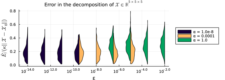
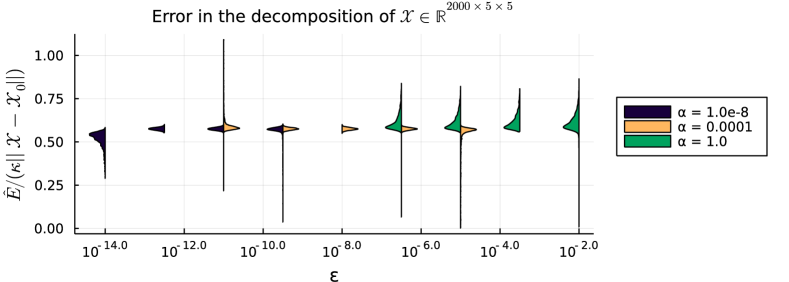
Figure 6.1. Distribution of $\frac{\widehat{E}}{\kappa\norm{{\mathpzc{X}}-{\mathpzc{X}}_{0}}_{F}}$ for a Tucker decomposition of the perturbed tensor ${\mathpzc{X}}$. An estimate of the probability density is plotted for all combinations of $(\alpha,\varepsilon)$ such that $90\%$ of samples satisfy $\widehat{E}\geq 5\times 10^{-8}$ and $90\%$ of samples satisfy $\kappa\norm{{\mathpzc{X}}-{\mathpzc{X}}_{0}}_{F}\leq 1$.

References

- [1] Ronny Bergmann “Manopt.jl: Optimization on Manifolds in Julia” In Journal of Open Source Software 7.70, 2022, pp. 3866 DOI: 10.21105/joss.03866
- [2] L. Blum, F. Cucker, M. Shub and S. Smale “Complexity and Real Computation” New York: Springer-Verlag, 1998
- [3] Paul Breiding and Nick Vannieuwenhoven “The Condition Number of Join Decompositions” In SIAM Journal on Matrix Analysis and Applications 39.1, 2018, pp. 287–309 DOI: 10.1137/17M1142880
- [4] Paul Breiding and Nick Vannieuwenhoven “The Condition Number of Riemannian Approximation Problems” arXiv: 1909.12186 In SIAM Journal on Optimization 31.1, 2021, pp. 1049–1077 DOI: 10.1137/20M1323527
- [5] Peter Bürgisser and Felipe Cucker “Condition” Series Title: Grundlehren der mathematischen Wissenschaften Publication Title: Media Berlin, Heidelberg: Springer Berlin Heidelberg, 2013 DOI: 10.1007/978-3-642-38896-5
- [6] Lieven De Lathauwer, Bart De Moor and Joos Vandewalle “A multilinear singular value decomposition” In SIAM Journal on Matrix Analysis and Applications 21.4, 2000, pp. 1253–1278 DOI: 10.1137/S0895479896305696
- [7] Jean-Pierre Dedieu “Approximate solutions of numerical problems, condition number analysis and condition number theorem” In The Mathematics of Numerical Analysis 32, Lectures in Applied Mathematics Park City, Utah, United States: American Mathematical Society, 1996, pp. 263–283
- [8] Jean-Pierre Dedieu and Myong-Hi Kim “Newton’s Method for Analytic Systems of Equations with Constant Rank Derivatives” In Journal of Complexity 18.1, 2002, pp. 187–209 DOI: 10.1006/jcom.2001.0612
- [9] James Demmel “On condition numbers and the distance to the nearest ill-posed problem” In Numerische Mathematik 51.3, 1987, pp. 251–289 DOI: 10.1007/BF01400115
- [10] Jérôme Dégot “A condition number theorem for underdetermined polynomial systems” In Mathematics of Computation 70.233, 2000, pp. 329–335 DOI: 10.1090/S0025-5718-00-00934-0
- [11] Wolfgang Hackbusch “Tensor Spaces and Numerical Tensor Calculus” 42, Springer Series in Computational Mathematics Berlin, Heidelberg: Springer Berlin Heidelberg, 2012 DOI: 10.1007/978-3-642-28027-6
- [12] Wolfgang Hackbusch and André Uschmajew “On the interconnection between the higher-order singular values of real tensors” In Numerische Mathematik 135.3, 2017, pp. 875–894 DOI: 10.1007/s00211-016-0819-9
- [13] Roger A. Horn and Charles R. Johnson “Topics in matrix analysis” Cambridge: Cambridge Univ. Press, 2010
- [14] M. Journée, F. Bach, P.-A. Absil and R. Sepulchre “Low-Rank Optimization on the Cone of Positive Semidefinite Matrices” In SIAM Journal on Optimization 20.5, 2010, pp. 2327–2351 DOI: 10.1137/080731359
- [15] Henk A. L. Kiers and Iven Van Mechelen “Three-way component analysis: Principles and illustrative application.” In Psychological Methods 6.1, 2001, pp. 84–110 DOI: 10.1037/1082-989X.6.1.84
- [16] Othmar Koch and Christian Lubich “Dynamical Tensor Approximation” In SIAM Journal on Matrix Analysis and Applications 31.5, 2010, pp. 2360–2375 DOI: 10.1137/09076578X
- [17] John M Lee “Introduction to Riemannian manifolds” Cham: Springer, 2018 URL: https://link.springer.com/book/10.1007/978-3-319-91755-9
- [18] John M. Lee “Introduction to Smooth Manifolds” Springer New York, 2013 DOI: 10.1007/978-1-4419-9982-5
- [19] Carla D. Moravitz Martin and Charles F. Van Loan “A Jacobi-Type Method for Computing Orthogonal Tensor Decompositions” In SIAM Journal on Matrix Analysis and Applications 30.3, 2008, pp. 1219–1232 DOI: 10.1137/060655924
- [20] I. V. Oseledets “Tensor-Train Decomposition” In SIAM Journal on Scientific Computing 33.5, 2011, pp. 2295–2317 DOI: 10.1137/090752286
- [21] John R. Rice “A Theory of Condition” In SIAM Journal on Numerical Analysis 3.2, 1966, pp. 287–310 DOI: 10.1137/0703023
- [22] Michael Shub and Steve Smale “Complexity of Bezout’s Theorem I: Geometric Aspects” In Journal of the American Mathematical Society 6.2, 1993, pp. 459 DOI: 10.2307/2152805
- [23] G.W Stewart and J.G Sun “Matrix perturbation theory” Publication Title: Mathematics and Computers in Simulation ISSN: 03784754 Academic Press, Inc., 1990 URL: https://linkinghub.elsevier.com/retrieve/pii/0378475491900385
- [24] Ledyard R Tucker “Some mathematical notes on three-mode factor analysis” In Psychometrika 31.3 Springer, 1966, pp. 279–311
- [25] Nick Vannieuwenhoven “Condition numbers for the tensor rank decomposition” In Linear Algebra and its Applications 535, 2017, pp. 35–86 DOI: 10.1016/j.laa.2017.08.014
- [26] Nick Vannieuwenhoven “The condition number of singular subspaces” arXiv preprint arXiv, 2022 URL: http://arxiv.org/abs/2208.08368
- [27] Nick Vannieuwenhoven, Raf Vandebril and Karl Meerbergen “A new truncation strategy for the higher-order singular value decomposition” In SIAM Journal on Scientific Computing 34.2, 2012, pp. 1027–1052 DOI: 10.1137/110836067