Renormalization of the gluon distribution function
in the background field formalism

Abstract

We derive the Leading Order DGLAP evolution of gluon distribution function in the target light cone gauge starting from its standard operator definition. The derivation is performed using the background field formalism employed in the Color Glass Condensate effective theory of small $x$ QCD. We adopt Mandelstam-Leibbrandt prescription to regulate in an unambiguous way the spurious singularity appearing in the light-cone gauge Feynman propagator. UV divergences are regulated via conventional dimensional regularization. The methods introduced in this paper represent the first steps in the construction of a unified framework for QCD evolution, which could address collinear physics as well as small $x$ physics and gluon saturation.

1 Introduction

pQCD-based collinear factorization formalism has been extremely successful in describing production of high $p_{t}$ particles in high energy collisions. If it can be proven for a class of processes it guarantees a clean separation of perturbative from non-perturbative dynamics up to power suppressed corrections. An essential ingredient in this approach is the evolution (scale dependence) of parton distribution functions which are calculable perturbatively in powers of $\alpha_{s}$. This evolution arises from renormalization of the parton distribution functions which exhibit the usual divergences present in relativistic quantum field theories. Nevertheless collinear factorization is expected to break down at very high energy (small $x$) due to the large gluon density in a proton or nucleus wave function generated by the fast rise of gluon distribution function. At such high gluon densities the concept of a quasi-free parton as envisioned by Feynman is not very useful and it may be more appropriate to describe this high occupancy state via semi-classical methods. Color Glass Condensate (CGC) formalism is an effective theory of QCD at small $x$ that uses classical color fields to describe such a high occupancy state (see [1, 2, 3] and references therein). In this formalism and in the context of dilute-dense collisions in the so-called hybrid approach, appropriate to the forward rapidity kinematics, one considers scattering of a projectile parton in a dilute proton on the dense system of gluons described as a classical color field. The typical momentum exchanged in such a scattering is of the order of the saturation scale $Q_{s}$ which roughly defines the border between dense and dilute regions of the target wave function. Such a formalism however can not be used at high transverse momenta since pQCD evolution of the hard scale becomes significant and one must use the collinear factorization formalism.

As the current and the proposed future colliders have a large phase space in $p_{t}$ and/or large $x$ it is imperative to try to combine the two approaches into one unified formalism that has both low $p_{t}$ (small $x$) and high $p_{t}$ (large $x$) dynamics built in. While there is an obvious need for and significant rewards for deriving such a unified formalism it is also a daunting task due to the complexities of the calculations involved as well as the fact that the underlying approximations and assumptions are vastly different. There is already some work done towards this goal [4, 5, 6] where one includes scattering of a projectile parton not only from small $x$ gluons of the target described by a classical color field, but also from large $x$ gluon field of the target. One loop corrections to this leading order result would then lead to an evolution equation which should reduce to DGLAP [7, 8, 9] and JIMWLK [10, 11, 12, 13, 14, 15, 16, 17] evolution equations in the appropriate limits.

The treatment introduced in [4, 5, 6] goes beyond the standard eikonal approximation that is frequently adopted in the CGC computations. Indeed, there has been a lot of efforts to include the subeikonal corrections in the CGC computations over the last decade. In Refs. [18, 19] a subset of subeikonal corrections to the gluon propagator are computed at next-to-next-to-eikonal order. The effects of these corrections on various observables in proton-proton and in proton-nucleus collisions are studied in [20, 21, 22, 23, 24]. Subeikonal corrections to the quark propagator and their applications to various DIS observables have been also studied at next-to-eikonal accuracy [25, 26, 27, 28]. In [29, 30, 31, 32, 33, 34, 35, 36, 37, 38, 39, 40, 41, 42, 43, 44] quark and gluon helicity evolutions have been computed for at next-to-eikonal accuracy. Subeikonal corrections to both quark and gluon propagators have been studied in the high-energy operator product expansion (OPE) formalism, and applied to study the polarized structure functions $g_{1}$ at low-$x$ in [45, 46]. Apart from the aforementioned direct studies of the subeikonal corrections, in [47, 48, 49, 50] rapidity evolution of transverse momentum dependent parton distributions (TMDs) that interpolates between the low and moderate energies have been studied. A similar idea has been pursued in [51, 52] for the unintegrated gluon distributions. Finally, effects of subeikonal corrections are studied in the context of orbital angular momentum in [53, 54].

The main goal of this paper is take the first steps towards understanding how the scale evolution of the collinear parton distributions can be embedded in the CGC effective theory of a dense target. We start with the standard operator definition of the gluon distribution function in the target light cone gauge and use the background field formalism to calculate the one loop corrections to the tree level result. Even though the target light cone gauge is not the standard one used in CGC but it is the standard gauge used in the collinear factorization framework where the parton model is manifest. Moreover, we use the Mandelstam-Leibbrandt (ML) prescription since it provides an unambiguous treatment of the spurious singularity appearing in the Feynman propagator in the light cone gauge [55, 56, 57]. As expected we encounter UV divergences which are then absorbed into the gluon distribution function leading to its scale dependence (evolution). Hence we show that DGLAP evolution of gluon distribution function corresponds to the standard UV renormalization of a composite operator constructed from the background fields of the CGC effective theory. Finally, we provide a summary of the results and discuss the outlook.

2 General definitions and setup

2.1 Gluon propagators in light-cone gauge

In the present study, we adopt the light-cone gauge

$$n\!\cdot\!A(x)= \,0$$ (1)

for the gluon field, where $n^{\mu}$ is a fixed light-like vector, meaning that $n^{2}=0$. By convention, $n^{\mu}$ is oriented towards the future ($n^{0}>1$).

The Feynman propagator for gluon in vacuum, defined as the time-ordered correlator

$$\langle 0|{\cal T}\left\{A_{a}^{\mu}(x)A_{b}^{\nu}(y)\right\}|0\rangle= \,\left[{\mathbb{1}}\right]_{ab}\;{G}_{0,F}^{\mu\nu}(x,y)=\left[{\mathbb{1}}\right]_{ab}\;\int\frac{d^{D}k}{(2\pi)^{D}}\,e^{-ik\cdot(x-y)}\,{\tilde{G}}_{0,F}^{\mu\nu}(k)\,,$$ (2)

is obtained in the light-cone gauge (1) as

$${\tilde{G}}_{0,F}^{\mu\nu}(k)= \,\frac{i}{\left(k^{2}+i0^{+}\right)}\,\left\{-g^{\mu\nu}+\frac{(k^{\mu}n^{\nu}+n^{\mu}k^{\nu})}{[n\!\cdot\!k]}\right\}$$ (3)

in momentum space. In addition to the usual $k^{2}$ denominator, regularized by the $+i0^{+}$ in the standard way for Feynman propagators, there is an extra denominator $[n\!\cdot\!k]$ which require a regularization as well, in order to fully specify the propagator (3). This issue is related to the residual gauge freedom, after imposing the light-cone gauge condition (1). In early studies in light-cone gauge QCD (in particular in Ref. [58]), the extra denominator was regularized with the Cauchy principal value. However, such regularization leads to various complications, such as preventing to perform Wick rotations, and the loss of power counting criterion for the convergence of Feynman integrals. A better regularization for that denominator, compatible with Wick rotations and power counting, is the Mandelstam-Leibbrandt (ML) prescription [55, 56], defined as

$$\frac{1}{[n\!\cdot\!k]}\equiv \,\frac{(\bar{n}\!\cdot\!k)}{(n\!\cdot\!k)(\bar{n}\!\cdot\!k)+i0^{+}}=\frac{1}{\left((n\!\cdot\!k)+i0^{+}\right)}\,\theta(\bar{n}\!\cdot\!k)+\frac{1}{\left((n\!\cdot\!k)-i0^{+}\right)}\,\theta(-\bar{n}\!\cdot\!k)\,,$$ (4)

where $\bar{n}^{\mu}$ is an additional light-like vector, with $\bar{n}^{2}=n^{2}=0$ and $\bar{n}\cdot n=1$. In Ref. [57], the Hamiltonian quantization of QCD has been performed in the light-cone gauge, leading unambiguously to the ML prescription (4) for the Feynman propagator. Interestingly, the Feynman propagator (3) with the ML prescription can be rewritten as

$${\tilde{G}}_{0,F}^{\mu\nu}(k)= \,\frac{i}{\left(k^{2}+i0^{+}\right)}\,\left\{-g^{\mu\nu}+\frac{2(\bar{n}\!\cdot\!k)}{{\mathbf{k}}^{2}}(k^{\mu}n^{\nu}+n^{\mu}k^{\nu})\right\}-\frac{i}{\big{(}2(n\!\cdot\!k)(\bar{n}\!\cdot\!k)+i0^{+}\big{)}}\,\frac{2(\bar{n}\!\cdot\!k)}{{\mathbf{k}}^{2}}\,(k^{\mu}n^{\nu}+n^{\mu}k^{\nu})$$ (5)

in which the second term can be interpreted as a ghost propagating along a light-like direction, resulting from the residual gauge freedom in the light-cone gauge [57].

In the present study, not only the free Feynman propagator is needed, but also the free Wightman propagator, defined as

$$\langle 0|A_{a}^{\mu}(x)A_{b}^{\nu}(y)|0\rangle= \,\left[{\mathbb{1}}\right]_{ab}\;{G}_{0,W}^{\mu\nu}(x,y)=\left[{\mathbb{1}}\right]_{ab}\;\int\frac{d^{D}k}{(2\pi)^{D}}\,e^{-ik\cdot(x-y)}\,{\tilde{G}}_{0,W}^{\mu\nu}(k)\,.$$ (6)

In momentum space, the Wightman propagator is related to the positive $k^{0}$ energy contribution to the discontinuity (when flipping $+i0^{+}$ to $-i0^{+}$) of the Feynman propagator, as

$${\tilde{G}}_{0,W}^{\mu\nu}(k)= \,\theta(k^{0})\;2\textrm{Re}\left({\tilde{G}}_{0,F}^{\mu\nu}(k)\right)\,.$$ (7)

Then, using eq. (5) and the Sochocki-Plemelj theorem, one obtains

$${\tilde{G}}_{0,W}^{\mu\nu}(k)= \,-g^{\mu\nu}\,\theta(\bar{n}\!\cdot\!k)\,2\pi\delta\left(k^{2}\right)+(k^{\mu}n^{\nu}+n^{\mu}k^{\nu})\frac{\theta(\bar{n}\!\cdot\!k)}{{\bf k}^{2}}\,2\pi\Big{[}\delta\Big{(}n\!\cdot\!k\!-\!\frac{{\bf k}^{2}}{2\bar{n}\!\cdot\!k}\Big{)}-\delta(n\!\cdot\!k)\Big{]}\,.$$ (8)

As a remark, in Ref. [59] the expressions (3) (with the ML prescription (4)) and (8) for gluon propagators in light-cone gauge been rederived in an axiomatic approach to QFT, requiring in particular causality, and formulated within distribution theory.

2.2 Operator definition of gluon distribution and target light-cone gauge

Let us consider a boosted hadronic target of momentum $P^{\mu}$, with a large light-cone component $n\!\cdot\!P=P^{-}$, where $n^{2}=0$. In general, the operator definition of the gluon distribution in that target is

$$G(\textrm{x}) =\frac{1}{\textrm{x}P^{-}}\int\frac{d\Delta x^{+}}{(2\pi)}\,e^{-i\textrm{x}P^{-}\Delta x^{+}}\,\langle P|F^{-i}_{b}(\Delta x^{+},0;0)\,U_{A}(\Delta x^{+},0)_{ba}\,F^{-i}_{a}(0,0;0)|P\rangle\,,$$ (9)

up to UV renormalization issues, where $\textrm{x}>0$ is the fraction of the momentum $P^{-}$ of the target carried by the gluon. In Eq. (9) the two field strength operators are connected in color by the adjoint gauge link operator

$$U_{A}(\Delta x^{+},0)= \,{\cal P}_{+}\exp\left\{-ig\int_{0}^{\Delta x^{+}}\!\!\!\!\!\!\!\!dz^{+}\,T^{c}\,A_{c}^{-}(z^{+},z^{-}=0;{\mathbf{z}}=0)\right\}\,,$$ (10)

where ${\cal P}_{+}$ indicates path ordering along the $z^{+}$ direction.

In the present study, for simplicity, we will restrict ourselves to the target light-cone gauge

$$n\!\cdot\!A(x)\equiv \,A^{-}(x)=0\,,$$ (11)

with the same light-like vector $n^{\mu}$ specifying both the gauge choice and the main component of the momentum of the target. With that gauge choice, the gauge link (10) reduces to the identity matrix, and Eq. (9) becomes

$$G(\textrm{x}) =\frac{1}{\textrm{x}P^{-}}\int\frac{d\Delta x^{+}}{(2\pi)}\,e^{-i\textrm{x}P^{-}\Delta x^{+}}\,\langle P|F^{-i}_{a}(\Delta x^{+},0;0)F^{-i}_{a}(0,0;0)|P\rangle\,.$$ (12)

Moreover, in the target light-cone gauge, the field strength tensor components with one upper $-$ index simplify as

$$F^{-\nu}(x)= \,\partial^{-}A^{\nu}(x)=\partial_{+}A^{\nu}(x)\,.$$ (13)

As a remark, since the target state with the same mometum $P^{\mu}$ is applied on the left and on the right of the operator, the phase factors generated when applying a translation to each field strength are compensating each other, and one has

$$\langle P|F^{-i}_{a}(\Delta x^{+},0;0)F^{-i}_{a}(0,0;0)|P\rangle= \,\langle P|F^{-i}_{a}(x^{+}\!+\!\Delta x^{+},0;0)F^{-i}_{a}(x^{+},0;0)|P\rangle=\langle P|F^{-i}_{a}(0,0;0)F^{-i}_{a}(-\Delta x^{+},0;0)|P\rangle\,.$$ (14)

Hence, Eq. (12) can be equivalently written as

$$G(\textrm{x}) =\frac{1}{\textrm{x}P^{-}}\int\frac{d\Delta x^{+}}{(2\pi)}\,e^{-i\textrm{x}P^{-}\Delta x^{+}}\,\langle P|F^{-i}_{a}(0,0;0)F^{-i}_{a}(-\Delta x^{+},0;0)|P\rangle$$

$$=\frac{1}{(2\pi)\textrm{x}P^{-}}\,\frac{1}{\left[\int dx^{+}\right]}\int dx^{+}\int dx^{\prime+}e^{-i\textrm{x}P^{-}(x^{\prime+}-x^{+})}\langle P|F^{-i}_{a}(x^{\prime+},0;0)F^{-i}_{a}(x^{+},0;0)|P\rangle\,.$$ (15)

The expression (15) has a clear interpretation if one adopts light-front quantization, with $n\!\cdot\!x=x^{-}$ replacing $x^{0}$ as evolution variable. Then, due to the sign in the phases in Eq. (15) (with $\textrm{x}P^{-}>0$), the partial Fourier transform selects the annihilation operator piece of the rightmost field strength and discard its creation operator piece. By contrast, the partial Fourier transform selects creation operator piece of the leftmost field strength, and discard its annihilation operator piece. Hence, the rightmost field strength in Eq. (15) removes a gluon with light-cone momentum $\textrm{x}P^{-}$ from the target, and the leftmost field strength adds it back. In particular, in light-front quantization along $n\!\cdot\!x=x^{-}$, all states have a positive (or vanishing) light-cone momentum $k^{-}$, so that it is not possible to remove a gluon with a momentum $\textrm{x}P^{-}$ larger than the total momentum $P^{-}$ of the target. For that reason,

$$\textrm{x}>1\;\Rightarrow\;G(\textrm{x})=0$$ (16)

so that the gluon distribution $G(\textrm{x})$ has a support $0\leq\textrm{x}\leq 1$. Although that property has been shown within light-front quantization, it should be valid in general, for any quantization procedure.

Finally, an important feature in the operator definition (12) of the gluon distribution is that the field strength operators are not time ordered (like in the Feynman propagator (2)) but are instead always in the same order, like in the Wightman propagator (6). In the Schwinger-Keldysh formalism, Wightman propagators can be interpreted as correlators between an operator in the amplitude and an operator in the complex conjugate amplitude, through the final-state cut, whereas Feynman propagators are correlators within amplitude only. This is consistent with the fact that collinear factorization and parton distributions arise only at the cross section level, not at amplitude level. Then, the rightmost field strength in the operator definition (12) should be intepreted as belonging to the amplitude, and the leftmost field strength as belonging to the complex conjugate amplitude.

2.3 Expansion around a background field

In order to calculate the evolution of the gluon distribution (12) induced by UV renormalization, we are using the background field method. Namely, we are splitting the gluon field into a background contribution and a fluctuation contribution, as

$$A^{\mu}(x) ={\cal A}^{\mu}(x)+\delta A^{\mu}(x)$$ (17)

at the gauge field level and

$$F^{\mu\nu}(x) ={\cal F}^{\mu\nu}(x)+\delta F^{\mu\nu}(x)$$ (18)

at the field strength level, and then we integrate over the fluctuation contribution to first order in the coupling $\alpha_{s}$ at the level of the gluon distribution. Since we apply the target light-cone gauge (2.3) both for the background and for the fluctuation fields, ${\cal A}^{-}(x)=0$ and $\delta A^{-}(x)=0$, one obtains both ${\cal F}^{-\nu}(x)=\partial_{+}{\cal A}^{\nu}(x)$ and $\delta{F}^{-\nu}(x)=\partial_{+}(\delta{A}^{\nu})(x)$.

First, by neglecting entirely the fluctuation field and keeping only the background field in the definition (12), one obtains what we call the bare contribution to the gluon distribution

$$G^{(0)}(\textrm{x}) =\frac{1}{\textrm{x}P^{-}}\int\frac{d\Delta x^{+}}{(2\pi)}\,e^{-i\textrm{x}P^{-}\Delta x^{+}}\,\langle P|{\cal F}^{-i}_{a}(\Delta x^{+},0;0){\cal F}^{-i}_{a}(0,0;0)|P\rangle\,.$$ (19)

Corrections beyond that bare contribution are obtained by expanding the correlator of two field strengths in the target hadron state as

$$\,\langle P|F_{a}^{-\mu}(x^{\prime})F_{a}^{-\nu}(x)|P\rangle-\langle P|{\cal F}_{a}^{-\mu}(x^{\prime}){\cal F}_{a}^{-\nu}(x)|P\rangle$$

$$\,=\langle P|{\cal F}_{a}^{-\mu}(x^{\prime})\delta F_{a}^{-\nu}(x)|P\rangle+\langle P|\delta F_{a}^{-\mu}(x^{\prime}){\cal F}_{a}^{-\nu}(x)|P\rangle+\langle P|\delta F_{a}^{-\mu}(x^{\prime})\delta F_{a}^{-\nu}(x)|P\rangle$$

$$\,=\partial_{x^{+}}\langle P|{\cal F}_{a}^{-\mu}(x^{\prime})\;\delta{A}_{a}^{\nu}(x)|P\rangle+\partial_{{x^{\prime}}^{+}}\langle P|\delta{A}_{a}^{\mu}(x^{\prime})\;{\cal F}_{a}^{-\nu}(x)|P\rangle+\partial_{{x^{\prime}}^{+}}\partial_{x^{+}}\langle P|\delta{A}_{a}^{\mu}(x^{\prime})\;\delta{A}_{a}^{\nu}(x)|P\rangle\,.$$ (20)

Each term in Eq. (20) can be expanded as a series both in the QCD coupling $g$ and in the background field.

First, let us first consider the contributions to the first two terms in Eq. (20) in which the fluctuation field $\delta{A}_{a}^{\nu}(x)$ is calculated (to all orders in $g$) at vanishing background field. This corresponds to the total vacuum tadpole contribution to $\delta{A}_{a}^{\nu}(x)$. By color symmetry, the color factor of any such tadpole diagram with one single adjoint index has to vanish. Hence, all non-trivial contributions to the first two terms in Eq. (20) are at least quadratic in the background field overall, with one power of the background field inserted inside the fluctuation $\delta{A}_{a}^{\nu}(x)$, beyond the explicit ${\cal F}_{a}^{-\mu}(x^{\prime})$ factor.

Let us now consider the third term in Eq. (20), at vanishing background field. Then, this correlator of fluctuations fields is the Wightman propagator in vacuum, but including corrections to all orders in $g$. When expanding in $g$ as well, the zeroth order contribution amounts simply to insert the free Wightman propagator (8) into Eq. (15), as

$$\,\frac{1}{(2\pi)\,\textrm{x}P^{-}\left[\int dx^{+}\right]}\int dx^{+}\int dx^{\prime+}e^{-i\textrm{x}P^{-}(x^{\prime+}-x^{+})}\partial_{{x^{\prime}}^{+}}\partial_{x^{+}}\;\left[{\mathbb{1}}\right]_{aa}\int\frac{d^{D}k}{(2\pi)^{D}}\>e^{-ik^{-}(x^{\prime+}-x^{+})}\;{\tilde{G}}_{0,W}^{ii}(k)$$

$$= \,\frac{(N_{c}^{2}\!-\!1)(\textrm{x}P^{-})^{2}}{(2\pi)\,\textrm{x}P^{-}}\int\frac{d^{D}k}{(2\pi)^{D}}\>2\pi\delta(k^{-}\!+\!\textrm{x}P^{-})\>(D\!-\!2)\,\theta(k^{+})\,2\pi\delta\left(2k^{+}k^{-}\!-\!{\mathbf{k}}^{2}\right)=0\,.$$ (21)

Indeed, the free Wightman propagator (8) imposes that $k^{-}\geq 0$ for a particle present at the final state cut, whereas both the Fourier transforms with respect to $x^{+}$ and $x^{\prime+}$ impose that $k^{-}<0$, since $\textrm{x}P^{-}>0$. This argument extends to all orders in $g$, for contributions independent of the background field. Indeed, at higher order in $g$, one typically has several particles at the final state cut, each described by a free Wightman propagator forcing its momentum to obey $k_{n}^{-}\geq 0$, whereas the Fourier transforms in $x^{+}$ and $x^{\prime+}$ forces the sum of these light-cone momenta to be strictly negative. In order to escape this argument, and obtain a non vanishing contribution to the gluon distribution from the third term in Eq. (20), one has to include background field insertions, in order to break the momentum conservation between the endpoints $x$ and $x^{\prime}$ of the correlator and the final state cut. More precisely, at least one background field insertion is required on each side of the final-state cut. For similar reasons, it is clear that in the first two terms in Eq. (20), contributions with all background field insertions on the same side of the cut will vanish at the level of the gluon distribution (15).

So far, we have shown that all non-zero contributions to the gluon distribution (15) in the expansion (17) around the background field and at any order in $g$ are at least quadratic in the background field, with at least one background field on each side of the cut, as expected for a parton distribution. In the following of the present study, we focus on the corrections which are exactly quadratic in the background field and of order $g^{2}$, in order to check that we recover the standard LO DGLAP evolution of the gluon distribution from its UV renormalization. At that order, from Eq. (20), we have

$$G(\textrm{x},\mu^{2}) =G^{(0)}(\textrm{x})+G(\textrm{x},\mu^{2})\bigg{|}_{\rm virt.ampl.}^{\rm NLO}+G(\textrm{x},\mu^{2})\bigg{|}_{\rm virt.cc.ampl}^{\rm NLO}+G(\textrm{x},\mu^{2})\bigg{|}_{\rm real}^{\rm NLO}+O({\cal F}^{3})+O(\alpha_{s}^{2})\,,$$ (22)

with the three NLO corrections beyond the bare term (19) coming respectively from the three terms in Eq. (20) and are represented diagrammatically on Fig. 1, and $O({\cal F}^{3})$ represents the corrections of higher order in the background field. We use conventional dimensional regularization (CDR) to deal with the UV divergences, and the gluon distribution becomes dependent on the CDR scale $\mu$.

                                                                                                                                                                                                                               

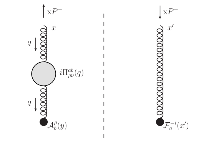
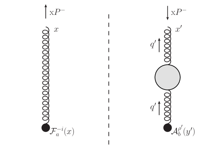
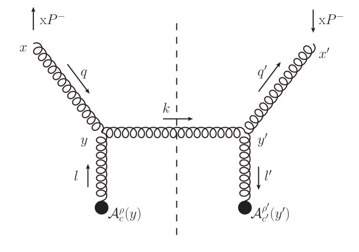
Figure 1: The three NLO corrections to the gluon distribution in the pure glue sector, see Eq. (22). In each diagram, the dashed line represent the final state cut.

The first NLO contribution in Eq. (22) amounts to correct the background field on the amplitude side by inserting the 1-loop vacuum polarization tensor, as

$$\delta A^{\mu}_{a}(x)\Big{|}_{\textrm{vac. pol.}}=\int\frac{d^{D}q}{(2\pi)^{D}}\,e^{iq\cdot x}\,{\tilde{G}}_{0,F}^{\nu\mu}(q)\;i\Pi_{\rho\nu}^{ba}(q)\;\int d^{D}y\,e^{-iy\cdot q}\,{\cal A}^{\rho}_{b}(y)\,,$$ (23)

so that

$$\delta F^{-\mu}_{a}(x)\Big{|}_{\textrm{vac. pol.}}=\partial_{x^{+}}\delta A^{\mu}_{a}(x)\Big{|}_{\textrm{vac. pol.}}=\int\frac{d^{D}q}{(2\pi)^{D}}\,e^{iq\cdot x}\,{\tilde{G}}_{0,F}^{\nu\mu}(q)\;i\Pi_{\rho\nu}^{ba}(q)\;\int d^{D}y\,e^{-iy\cdot q}\,{\cal F}^{-\rho}_{b}(y)\,,$$ (24)

in the target light-cone gauge . At the level of the gluon distribution, this correction corresponds to

$$G(\textrm{x},\mu^{2})\bigg{|}_{\rm virtual;\,ampl.}^{\rm NLO}= \,\frac{1}{(2\pi)\textrm{x}P^{-}}\,\frac{1}{\left[\int dx^{+}\right]}\int dx^{+}\int dx^{\prime+}e^{-i\textrm{x}P^{-}(x^{\prime+}-x^{+})}\int\frac{d^{D}q}{(2\pi)^{D}}\,e^{iq^{-}x^{+}}\,{\tilde{G}}_{0,F}^{\nu i}(q)\;i\Pi_{\rho\nu}^{ba}(q)\;$$

$$\,\hskip 113.81102pt\times\;\int d^{D}y\,e^{-iy\cdot q}\,\langle P|{\cal F}^{-i}_{a}(x^{\prime+},0;0){\cal F}^{-\rho}_{b}(y)|P\rangle$$

$$= \,\int\frac{d^{D}q}{(2\pi)^{D}}\,\frac{2\pi\delta(q^{-}\!+\!\textrm{x}P^{-})}{(2\pi)\textrm{x}P^{-}}\;{\tilde{G}}_{0,F}^{\nu i}(q)\;i\Pi^{ba}_{\rho\nu}(q)\int d^{D}\Delta y\,e^{iq\cdot\Delta y}\,\langle P|{\cal F}^{-i}_{a}(0){\cal F}^{-\rho}_{b}(-\Delta y)|P\rangle$$ (25)

using the invariance by translation of the matrix element (14) at zero momentum transfer. The contribution of the second diagram on Fig. 1, with the vacuum polarization tensor inserted on the leftmost field strength, or equivalently on the complex conjugate amplitude side is analog to the contribution (25). The calculation of the one-loop vacuum polarization tensor is presented in Sec. (4), as well as the evaluation of contribution (25) to the gluon distribution at NLO.

The third NLO contribution in Eq. (22), represented by the third diagram on Fig. 1, can be written as

$$G(\textrm{x},\mu^{2})\bigg{|}_{\rm real}^{\rm NLO}=\frac{(\textrm{x}P^{-})^{2}}{(2\pi)\,\textrm{x}P^{-}\left[\int dx^{+}\right]}\int dx^{+}\int dx^{\prime+}e^{-i\textrm{x}P^{-}(x^{\prime+}-x^{+})}\delta^{ii^{\prime}}\left[{\mathbb{1}}\right]_{aa^{\prime}}\,\langle P|\,\delta A^{i^{\prime}}_{a^{\prime}}(x^{\prime+},0;0)\delta A^{i}_{a}(x^{+},0;0)|P\rangle\bigg{|}_{{\cal A}{\cal A}}\,,$$ (26)

in which the correlator is the contribution to the gluon Wightman propagator in the in the target state with two insertions of the target background field strength, one on each side of the final state cut. The contribution (26) to the gluon distribution at is evaluated in section 3.

3 Real contributions

We now calculate the real diagram shown as the third diagram on Fig. (1), corresponding to Eq. (26) and show how it contributes to the DGLAP evolution of the gluon distribution function defined above. We use the standard Feynman rules of QCD and write our expressions in $D$-dimensions with the dimensionful parameter $\mu$ included since we use dimensional regularization to regulate the divergences that are expected to arise. The main building block in Eq. (26) in the Wightman propagator with two insertions of the gluon background field of the target, one on each side of the cut. It can be written as

$$\,\langle P|\delta A^{i^{\prime}}_{a^{\prime}}(x^{\prime})\delta A^{i}_{a}(x)|P\rangle\bigg{|}_{{\cal A}{\cal A}}=\int\frac{d^{D}q}{(2\pi)^{D}}\int\frac{d^{D}k}{(2\pi)^{D}}\int\frac{d^{D}q^{\prime}}{(2\pi)^{D}}\int d^{D}y\int d^{D}y^{\prime}\;e^{-iq^{\prime}\cdot x^{\prime}}\,e^{iq\cdot x}\,e^{iy\cdot(k-q)}\,e^{-iy^{\prime}\cdot(k-q^{\prime})}$$

$$\,\times\;{\tilde{G}}_{0,\bar{F}}^{i^{\prime}\nu^{\prime}}(q^{\prime})\,(-1){V_{3g}}_{\nu^{\prime}\sigma^{\prime}\rho^{\prime}}^{a^{\prime}bc^{\prime}}(-q^{\prime},k,q^{\prime}\!-\!k)\;{\tilde{G}}_{0,W}^{\sigma^{\prime}\sigma}(k){V_{3g}}_{\nu\sigma\rho}^{abc}(q,-k,k\!-\!q)\;{\tilde{G}}_{0,F}^{\nu i}(q)\;\langle P|{\cal A}^{\rho^{\prime}}_{c^{\prime}}(y^{\prime})\,{\cal A}^{\rho}_{c}(y)|P\rangle$$ (27)

Note that only the propagator of momentum $q$ is entirely on the amplitude side, and is thus a free Feynman propagator given by Eq. (3). By contrast, the propagator of momentum $k$ crosses the final state cut, and is thus the free Wightman propagator given by Eq. (8). Finally, the propagator of momentum $q^{\prime}$ is entirely on the complex conjugate amplitude side of the cut. It is thus an anti-time-ordered propagator. In momentum space, this is simply the complex conjugate of the corresponding time-ordered Feynman propagator,

$${\tilde{G}}_{0,\bar{F}}^{\mu\nu}(p)= \,\left({\tilde{G}}_{0,F}^{\mu\nu}(p)\right)^{{\dagger}}\,.$$ (28)

The real diagram from Fig. (1) contains two standard three-gluon vertices. However, one is on each side of the final state cut. The one on the complex conjugate amplitude side comes with an extra $(-1)$ factor, following the standard Schwinger-Keldysh formalism.

We can rewrite the expression (27) in terms of gluon field strength tensors by multiplying and dividing by factors of ($k^{-}\!-\!q^{-}$) and ($k^{-}\!-\!q^{-\,\prime}$). One can then convert these momenta into derivatives with respect to $y^{+}$ and $y^{\prime\,+}$ acting on the fields ${\cal A}^{\rho}_{c}(y)$ and ${\cal A}^{\rho^{\prime}}_{c^{\prime}}(y^{\prime})$ after integration by parts, which in the light-cone gauge correspond to background field strengths. We also use the invariance by translation of the correlation function (see Eq. (14)) in order to write it as a function of the separation $\Delta y\equiv y^{\prime}-y$ between the fields only. This allows us to to integrate over the ”center of mass” coordinate $y+y^{\prime}$ and use the resulting delta function to integrate over momentum $q^{\prime}$ which sets it equal to $q$. This leads to

$$\langle P|\delta A^{i^{\prime}}_{a^{\prime}}(x^{\prime})\delta A^{i}_{a}(x)|P\rangle\bigg{|}_{{\cal A}{\cal A}}=2g^{2}\,\mu^{2\epsilon}\,f^{abc}\,f^{a^{\prime}bc^{\prime}}\int\frac{d^{D}q}{(2\pi)^{D}}\,\int\frac{d^{D}k}{(2\pi)^{D}}\,{\tilde{G}}^{i^{\prime}\nu^{\prime}}_{0,\bar{F}}(q)\,{\tilde{G}}^{\sigma^{\prime}\sigma}_{0,W}(k)\,{\tilde{G}}_{0,F}^{\nu i}(q)$$

$$\times\Big{[}(q_{\rho}+k_{\rho})g_{\nu\sigma}+(q_{\nu}-2k_{\nu})g_{\sigma\rho}+(k_{\sigma}-2q_{\sigma})g_{\nu\rho}\Big{]}\Big{[}(q_{\rho^{\prime}}+k_{\rho^{\prime}})g_{\nu^{\prime}\sigma^{\prime}}+(q_{\nu^{\prime}}-2k_{\nu^{\prime}})g_{\sigma^{\prime}\rho^{\prime}}+(k_{\sigma^{\prime}}-2q_{\sigma^{\prime}})g_{\nu^{\prime}\rho^{\prime}}\Big{]}$$

$$\times\frac{e^{-iq\cdot(x^{\prime}-x)}}{(k^{-}-q^{-})^{2}}\int d^{D}\Delta y\,e^{-i(k-q)\cdot\Delta y}\,\langle P|{\cal F}^{-\rho^{\prime}}_{c^{\prime}}(\Delta y){\cal F}^{-\rho}_{c}(0)|P\rangle\,,$$ (29)

where $D=4-2\epsilon$.

Next, we insert the expression (29) into Eq. (26) and integrate over $x^{+}$ and $x^{\prime+}$. To proceed further we make the assumption that the field strength correlator does not depend on the $\Delta y^{-}$ coordinate. Indeed, such dependence is a power suppressed effect in the high-energy limit [26] which should not be relevant in the derivation of the DGLAP evolution. At this stage, one obtains

$$G(\textrm{x},\mu^{2})\bigg{|}^{\rm NLO}_{\rm real}=\frac{g^{2}\,C_{A}\,\mu^{2\epsilon}}{(2\pi)\,\textrm{x}P^{-}}\,\int\frac{d^{D}k}{(2\pi)^{D}}\,\left(\frac{\textrm{x}P^{-}}{k^{-}\!+\!\textrm{x}P^{-}}\right)^{2}\int d\Delta y^{+}\int d^{D-2}\Delta{\bf y}\langle P|{\cal F}^{-\rho^{\prime}}_{a}(\Delta y^{+},0;\Delta{\bf y}){\cal F}^{-\rho}_{a}(0,0;0)|P\rangle$$

$$\times\int\frac{d^{D}q}{(2\pi)^{D}}\,2\pi\delta(q^{+}\!-\!k^{+})\,2\pi\delta(q^{-}\!+\!\textrm{x}P^{-})\,e^{-i(k^{-}+\textrm{x}P^{-})\Delta y^{+}}\,e^{i(\bf k-\bf q)\cdot{\bf\Delta y}}\frac{{\tilde{G}}^{\sigma^{\prime}\sigma}_{0,W}(k)}{\big{[}-2\textrm{x}P^{-}k^{+}-{\bf q}^{2}+i0^{+}\big{]}\big{[}-2\textrm{x}P^{-}k^{+}-{\bf q}^{2}-i0^{+}\big{]}}$$

$$\times\bigg{\{}-g_{\sigma}^{\;\;i}(q_{\rho}\!+\!k_{\rho})-g_{\rho}^{\;\;i}(k_{\sigma}\!-\!2q_{\sigma})+2g_{\sigma\rho}\bigg{[}{\bf k}^{i}\!-\!\frac{k^{-}}{q^{-}}{\bf q}^{i}\bigg{]}\bigg{\}}\bigg{\{}-g_{\sigma^{\prime}}^{\;\;i}(q_{\rho^{\prime}}\!+\!k_{\rho^{\prime}})-g_{\rho^{\prime}}^{\;\;i}(k_{\sigma^{\prime}}\!-\!2q_{\sigma^{\prime}})+2g_{\sigma^{\prime}\rho^{\prime}}\bigg{[}{\bf k}^{i}\!-\!\frac{k^{-}}{q^{-}}{\bf q}^{i}\bigg{]}\bigg{\}}$$ (30)

Due to the specific form of the cut propagator in Eq. (8), it is more convenient to consider the two parts of the cut propagator separately, labeled as metric and gauge parts. We first consider the gauge part, simplifying the Lorentz algebra and using the delta functions to perform the $q^{+},q^{-}$ integrals leads to

$$G(\textrm{x},\mu^{2})\bigg{|}^{\rm NLO}_{\rm real;gauge\,art.}=\frac{g^{2}\,C_{A}\,\mu^{2\epsilon}}{(2\pi)\,\textrm{x}P^{-}}\,\int d\Delta y^{+}\int d^{D-2}\Delta{\bf y}\;\langle P|{\cal F}^{-\rho^{\prime}}_{a}(\Delta y^{+},0;\Delta{\bf y}){\cal F}^{-\rho}_{a}(0,0;0)|P\rangle$$

$$\times\int\frac{d^{D}k}{(2\pi)^{D}}\,e^{-i(k^{-}+\textrm{x}P^{-})\Delta y^{+}}\,\left(\frac{\textrm{x}P^{-}}{k^{-}\!+\!\textrm{x}P^{-}}\right)^{2}\,\int\frac{d^{D-2}{\bf q}}{(2\pi)^{D-2}}\,\frac{e^{i({\bf k}-\bf q)\cdot\Delta{\bf y}}}{(2\textrm{x}P^{-}k^{+}+{\bf q}^{2})^{2}}\,\frac{\theta(k^{+})}{{\bf k}^{2}}\,2\pi\Big{[}\delta\Big{(}k^{-}-\frac{{\bf k}^{2}}{2k^{+}}\Big{)}-\delta(k^{-})\Big{]}$$

$$\times(k^{-}+2\textrm{x}P^{-})\Big{\{}2g_{\rho}^{\;\;i}g_{\rho^{\prime}}^{\;\;i}\big{[}2\textrm{x}P^{-}k^{+}+{\bf q}^{2}-({\bf k}-{\bf q})^{2}\big{]}+\big{(}g_{\rho}^{\;\;i}g_{\rho^{\prime}}^{\;\;j}+g_{\rho}^{\;\;j}g_{\rho^{\prime}}^{\;\;i}\big{)}\Big{[}{\bf k}^{i}({\bf k}^{j}-{\bf q}^{j})+\frac{2k^{-}}{\textrm{x}P^{-}}{{\bf q}^{i}}{\bf k}^{j}\Big{]}$$

$$\hskip 73.97733pt+\big{(}g_{\rho}^{\;\;i}g_{\rho^{\prime}}^{\;\;+}+g_{\rho}^{\;\;+}g_{\rho^{\prime}}^{\;\;i}\big{)}\Big{[}-2k^{-}\Big{(}{\bf k}^{i}+\frac{k^{-}}{\textrm{x}P^{-}}{\bf q}^{i}\Big{)}+(k^{-}\!-\!\textrm{x}P^{-}){\bf k}^{i}\Big{]}\Big{\}}$$ (31)

We now introduce the momentum fraction $z$ defined as

$$z=\frac{\textrm{x}P^{-}}{\big{[}\textrm{x}P^{-}+\frac{{\bf k}^{2}}{2k^{+}}\big{]}}$$ (32)

and perform changes of variables from $k^{+}$ to $z$, and from the transverse momenta ${\bf k}$ and ${\bf q}$ to

$${\bf l} ={\bf k}-{\bf q}$$ (33)

$${\bf K} =z{\bf k}+(1-z){\bf q}$$ (34)

to make the above expression more tractable, and we get

$$G(\textrm{x},\mu^{2})\bigg{|}^{\rm NLO}_{\rm real;gauge\,art.}=\frac{\alpha_{s}\,C_{A}}{(2\pi)\,\textrm{x}P^{-}}\,\int d\Delta y^{+}\int d^{2-2\epsilon}\Delta{\bf y}\;\langle P|{\cal F}^{-\rho^{\prime}}_{a}(\Delta y^{+},0;\Delta{\bf y}){\cal F}^{-\rho}_{a}(0,0;0)|P\rangle\int_{0}^{1}dz$$

$$\times\int\frac{d^{2-2\epsilon}{\bf l}}{(2\pi)^{2-2\epsilon}}\,e^{i{\bf l}\cdot\Delta{\bf y}}\mu^{2\epsilon}\int\frac{d^{2-2\epsilon}\,{\bf K}}{(2\pi)^{2-2\epsilon}}\,\frac{1}{[{\bf K}^{2}+z(1-z){\bf l}^{2}]^{2}}\bigg{\{}z(1+z)\theta(z-\textrm{x})\,e^{-i\frac{\textrm{x}P^{-}}{z}\Delta y^{+}}\bigg{[}2g_{\rho}^{\;\;i}g_{\rho^{\prime}}^{\;\;i}\bigg{(}\frac{{\bf K}^{2}+z(1-z){\bf l}^{2}}{(1-z)}-{\bf l}^{2}\bigg{)}$$

$$+\big{(}g_{\rho}^{\;\;i}g_{\rho^{\prime}}^{\;\;j}+g_{\rho}^{\;\;j}g_{\rho^{\prime}}^{\;\;i}\big{)}\bigg{(}(1-z){\bf l}^{i}{\bf l}^{j}+\frac{2(1-z)}{z}\Big{[}{\bf K}^{i}{\bf K}^{j}-z(1-z){\bf l}^{i}{\bf l}^{j}\Big{]}\bigg{)}+\big{(}g_{\rho}^{\;\;i}g_{\rho^{\prime}}^{\;\;+}+g_{\rho}^{\;\;+}g_{\rho^{\prime}}^{\;\;i}\big{)}\textrm{x}P^{-}\frac{(1-2z)(1-z)}{z}\bigg{]}$$

$$-2e^{-i\textrm{x}P^{-}\Delta y^{+}}\bigg{[}2g_{\rho}^{\;\;i}g_{\rho^{\prime}}^{\;\;i}\bigg{(}\frac{{\bf K}^{2}+z(1-z){\bf l}^{2}}{(1-z)}-{\bf l}^{2}\bigg{)}+\big{(}g_{\rho}^{\;\;i}g_{\rho^{\prime}}^{\;\;j}+g_{\rho}^{\;\;j}g_{\rho^{\prime}}^{\;\;i}\big{)}(1-z){\bf l}^{i}{\bf l}^{j}-\big{(}g_{\rho}^{\;\;i}g_{\rho^{\prime}}^{\;\;+}+g_{\rho}^{\;\;+}g_{\rho^{\prime}}^{\;\;i}\big{)}\textrm{x}P^{-}(1-z){\bf l}^{i}\bigg{]}\bigg{\}}$$ (35)

The integral over transverse momentum ${\bf K}$ can now be carried out using the standard techniques of dimensional regularization. As we are interested in evolution of the gluon distribution function to Leading Order accuracy we only need the UV divergent pieces of the integral which appears as a $\frac{1}{\epsilon}$ pole, inducing a logarithmic dependence on the scale $\mu$.

$$G(\textrm{x},\mu^{2})\bigg{|}^{\rm NLO}_{\rm real;gauge\,art.\,;\,UV} =\frac{\alpha_{s}\,C_{A}}{(4\pi)(2\pi)\,\textrm{x}P^{-}}\,\int d\Delta y^{+}\int d^{2-2\epsilon}\Delta{\bf y}\;\langle P|{\cal F}^{-\rho^{\prime}}_{a}(\Delta y^{+},0;\Delta{\bf y}){\cal F}^{-\rho}_{a}(0,0;0)|P\rangle$$

$$\times\int_{0}^{1}dz\int\frac{d^{2-2\epsilon}\,{\bf l}}{(2\pi)^{2-2\epsilon}}\,e^{i{\bf l}\cdot\Delta{\bf y}}\,\frac{\Gamma(1+\epsilon)}{\epsilon}\,\bigg{[}\frac{z(1-z){\bf l}^{2}}{4\pi\mu^{2}}\bigg{]}^{-\epsilon}\bigg{\{}z(1+z)e^{-i\frac{\textrm{x}P^{-}}{z}\Delta y^{+}}\theta(z-\textrm{x})$$

$$\times\bigg{[}\frac{2}{(1-z)}g_{\rho}^{\;\;i}g_{\rho^{\prime}}^{\;\;i}+\big{(}g_{\rho}^{\;\;i}g_{\rho^{\prime}}^{\;\;j}+g_{\rho}^{\;\;j}g_{\rho^{\prime}}^{\;\;i}\big{)}\frac{2(1-z)}{z}\frac{\delta^{ij}}{2(1-\epsilon)}\bigg{]}-2e^{-i\textrm{x}P^{-}\Delta y^{+}}\frac{2}{(1-z)}g_{\rho}^{\;\;i}g_{\rho^{\prime}}^{\;\;i}\bigg{\}}$$ (36)

Note that the $\theta(z-\textrm{x})$ is obtained from the property (16), due to the dependence on $\textrm{x}P^{-}/z$ instead of $\textrm{x}P^{-}$ in the phase.

The UV divergent piece (with its accompanying $\mu^{2\epsilon}$ factor) is independent of the internal transverse momentum ${\bf l}$ which then allows us to perform the integral over ${\bf l}$ resulting in a delta function of transverse distances. This forces the transverse separation $\Delta{\bf y}$ between the two field strength tensors to go to zero as is the case in the standard definition of the gluon distribution function. It is important to notice that we have not made this assumption but that it is the result of the calculation. Defining the $+$ prescription as

$$\int_{\textrm{x}}^{1}dz\,\frac{f(z)}{(1-z)_{+}}\equiv \,\int_{0}^{1}dz\,\frac{\left[f(z)\theta(z\!-\!\textrm{x})-f(1)\right]}{(1-z)}$$ (37)

as usual, the contribution of the gauge dependent piece of the cut propagator the evolution of gluon distribution function can then be written as

$$G(\textrm{x},\mu^{2})\bigg{|}^{\rm NLO}_{\rm real;gauge\,art.\,;\,UV} =\frac{\alpha_{s}\,C_{A}}{\pi}\,\left\{\frac{\mu^{2\epsilon}}{\epsilon}\int_{\textrm{x}}^{1}\frac{dz}{z}\frac{1}{2}\bigg{[}\frac{z(1+z)}{(1-z)_{+}}+1-z^{2}\bigg{]}G^{(0)}\Big{(}\frac{\textrm{x}}{z}\Big{)}+O(\epsilon^{0})\right\}$$ (38)

where the factors common with the tree level definition in Eq. (19) are factored out. Eq. (38) represents the UV contribution of the gauge dependent part of the cut propagator (8) in the real NLO correction to the gluon distribution function.

We now consider the contribution of the metric part of the free Wightman propagator, Eq. (8) to the real NLO diagram. Most of the intermediate steps are identical to the gauge dependent part that was shown in great detail. After doing some of the momentum integrations using the delta functions we get

$$G(\textrm{x},\mu^{2})\bigg{|}^{\rm NLO}_{\rm real;\,metric} =\frac{g^{2}\,C_{A}\,\mu^{2\epsilon}}{(2\pi)\,\textrm{x}P^{-}}\int d\Delta y^{+}\int d^{2-2\epsilon}\Delta{\bf y}\,\langle P|{\cal F}^{-\rho^{\prime}}_{a}(\Delta y^{+},0;\Delta{\bf y}){\cal F}^{-\rho}_{a}(0,0;0)|P\rangle$$

$$\times\int\frac{d^{4-2\epsilon}\,k}{(2\pi)^{4-2\epsilon}}\,2\pi\delta\Big{(}k^{+}-\frac{{\bf k}^{2}}{2k^{-}}\Big{)}\,\frac{\theta(k^{-})}{2k^{-}}\bigg{(}\frac{\textrm{x}P^{-}}{k^{-}+\textrm{x}P^{-}}\bigg{)}^{2}\,e^{-i(k^{-}+\textrm{x}P^{-})\Delta y^{+}}\int\frac{d^{2-2\epsilon}\,{\bf q}}{(2\pi)^{2-2\epsilon}}\frac{e^{i({\bf k}-{\bf q})\cdot\Delta{\bf y}}}{[2\textrm{x}P^{-}k^{+}+{\bf q}^{2}]^{2}}$$

$$\times\bigg{\{}g_{\rho}^{\;\;i}g_{\rho^{\prime}}^{\;\;i}\bigg{[}4\Big{(}{\bf k}+\frac{k^{-}}{\textrm{x}P^{-}}{\bf q}\Big{)}^{2}+2\Big{(}2\textrm{x}P^{-}k^{+}+{\bf q}^{2}\Big{)}+2({\bf k}-{\bf q})^{2}\bigg{]}+2(1-\epsilon)(k^{-}-\textrm{x}P^{-})^{2}g_{\rho}^{\;\;+}g_{\rho^{\prime}}^{\;\;+}$$

$$\hskip 17.07182pt+\big{(}g_{\rho}^{\;\;i}g_{\rho^{\prime}}^{\;\;j}+g_{\rho}^{\;\;j}g_{\rho^{\prime}}^{\;\;i}\big{)}\bigg{[}\bigg{(}{\bf q}^{i}+{\bf k}^{i}-2\Big{(}{\bf k}^{i}+\frac{k^{-}}{\textrm{x}P^{-}}{\bf q}^{i}\Big{)}\bigg{)}(2{\bf k}^{j}-{\bf q}^{j})-\epsilon({\bf k}^{i}+{\bf q}^{i})({\bf k}^{j}+{\bf q}^{j})\bigg{]}$$

$$\hskip 17.07182pt+\big{(}g_{\rho}^{\;\;i}g_{\rho^{\prime}}^{\;\;+}+g_{\rho}^{\;\;+}g_{\rho^{\prime}}^{\;\;i}\big{)}\bigg{[}2(2k^{-}\textrm{x}P^{-})\Big{(}{\bf k}^{i}+\frac{k^{-}}{\textrm{x}P^{-}}{\bf q}^{i}\Big{)}-(k^{-}-\textrm{x}P^{-})\Big{(}3{\bf k}^{i}-2\epsilon({\bf q}^{i}+{\bf k}^{i})\Big{)}\bigg{]}\bigg{\}}$$ (39)

In this case, we can define the momentum fraction $z$ as

$$z=\frac{\textrm{x}P^{-}}{k^{-}+\textrm{x}P^{-}}$$ (40)

for simplicity and perform changes of variables from $k^{-}$ to $z$ and then from transverse momenta (${\bf k},{\bf q}$) to (${\bf K},{\bf l}$) as before, to get

$$G(\textrm{x},\mu^{2})\bigg{|}^{\rm NLO}_{\rm real;\,metric} =\frac{\alpha_{s}\,C_{A}}{(2\pi)\,\textrm{x}P^{-}}\int_{\textrm{x}}^{1}dz\,\int d\Delta y^{+}\,e^{-i\frac{\textrm{x}P^{-}}{z}\Delta y^{+}}\int d^{2-2\epsilon}\Delta{\bf y}\,\langle P|{\cal F}^{-\rho^{\prime}}_{a}(\Delta y^{+},0;\Delta{\bf y}){\cal F}^{-\rho}_{a}(0,0;0)|P\rangle$$

$$\times\int\frac{d^{2-2\epsilon}\,{\bf l}}{(2\pi)^{2-2\epsilon}}\,e^{i{\bf l}\cdot\Delta{\bf y}}\,\mu^{2\epsilon}\int\frac{d^{2-2\epsilon}\,{\bf K}}{(2\pi)^{2-2\epsilon}}\,\frac{z(1-z)}{[{\bf K}^{2}+z(1-z){\bf l}^{2}]^{2}}$$

$$\times\bigg{\{}g_{\rho}^{\;\;i}g_{\rho^{\prime}}^{\;\;i}\bigg{[}4\frac{{\bf K}^{2}}{z^{2}}+\frac{2}{(1-z)}\Big{(}{\bf K}^{2}+z(1-z){\bf l}^{2}\Big{)}+2{\bf l}^{2}\bigg{]}+2(1-\epsilon)\frac{(1-2z)^{2}}{z^{2}}(\textrm{x}P^{-})^{2}g_{\rho}^{\;\;+}g_{\rho^{\prime}}^{\;\;+}$$

$$\hskip 17.07182pt+\big{(}g_{\rho}^{\;\;i}g_{\rho^{\prime}}^{\;\;j}+g_{\rho}^{\;\;j}g_{\rho^{\prime}}^{\;\;i}\big{)}\Big{[}-2\frac{(1-z)}{z}{\bf K}^{i}{\bf K}^{j}+(1-2z)(2-z){\bf l}^{i}{\bf l}^{j}-4\epsilon\,{\bf K}^{i}{\bf K}^{j}-\epsilon(1-2z)^{2}{\bf l}^{i}{\bf l}^{j}\Big{]}$$

$$\hskip 17.07182pt+\big{(}g_{\rho}^{\;\;i}g_{\rho^{\prime}}^{\;\;+}+g_{\rho}^{\;\;+}g_{\rho^{\prime}}^{\;\;i}\big{)}\frac{\textrm{x}P^{-}}{z}(-1)(1-2z){\bf l}^{i}\big{[}3(1-z)-2\epsilon(1-2z)\big{]}\bigg{\}}$$ (41)

The transverse momentum integration over ${\bf K}$ can be again carried out using dimensional regularization techniques and gives the UV divergent piece of the integral as

$$G(\textrm{x},\mu^{2})\bigg{|}^{\rm NLO}_{\rm real;\,metric;\,UV} =\frac{\alpha_{s}\,C_{A}}{(2\pi)\,\textrm{x}P^{-}}\int_{\textrm{x}}^{1}dz\,\int d\Delta y^{+}\,e^{-i\frac{\textrm{x}P^{-}}{z}\Delta y^{+}}\int d^{2-2\epsilon}\Delta{\bf y}\,\langle P|{\cal F}^{-\rho^{\prime}}_{a}(\Delta y^{+},0;\Delta{\bf y}){\cal F}^{-\rho}_{a}(0,0;0)|P\rangle$$

$$\times\int\frac{d^{2-2\epsilon}\,{\bf l}}{(2\pi)^{2-2\epsilon}}\,e^{i{\bf l}\cdot\Delta{\bf y}}\,\frac{1}{4\pi}z(1-z)\frac{\Gamma(1+\epsilon)}{\epsilon}\bigg{[}\frac{z(1-z){\bf l}^{2}}{4\pi\mu^{2}}\bigg{]}^{-\epsilon}$$

$$\times\bigg{\{}g_{\rho}^{\;\;i}g_{\rho^{\prime}}^{\;\;i}\bigg{[}\frac{4}{z^{2}}+\frac{2}{(1-z)}\bigg{]}+\big{(}g_{\rho}^{\;\;i}g_{\rho^{\prime}}^{\;\;j}+g_{\rho}^{\;\;j}g_{\rho^{\prime}}^{\;\;i}\big{)}\frac{\delta^{ij}}{2(1-\epsilon)}\bigg{[}-2\frac{(1-z)}{z}-4\epsilon\bigg{]}\bigg{\}}$$ (42)

As before the divergent piece of the result is independent of the intrinsic transverse momentum ${\bf l}$ which allows one to perform the ${\bf l}$ integral forcing $\Delta{\bf y}\rightarrow 0$. The UV divergent piece of the contributions of the metric part of the cut propagator can then be written as

$$G(\textrm{x},\mu^{2})\bigg{|}^{\rm NLO}_{\rm real;\,metric;\,UV} =\frac{\alpha_{s}\,C_{A}}{\pi}\,\left\{\frac{\mu^{2\epsilon}}{\epsilon}\int_{\textrm{x}}^{1}\frac{dz}{z}\bigg{[}\frac{(1-z)}{z}+\frac{z}{2}-\frac{(1-z)^{2}}{2}\bigg{]}G^{(0)}\Big{(}\frac{\textrm{x}}{z}\Big{)}+O(\epsilon^{0})\right\}$$ (43)

Adding this to the UV divergent piece of the contributions of the gauge dependent part as given in Eq. (38) the total UV contribution by the real diagram is

$$G(\textrm{x},\mu^{2})\bigg{|}^{\rm NLO}_{\rm real;\,UV} =\frac{\alpha_{s}\,C_{A}}{\pi}\,\left\{\frac{\mu^{2\epsilon}}{\epsilon}\int_{\textrm{x}}^{1}\frac{dz}{z}\bigg{[}\frac{z}{(1-z)_{+}}+\frac{(1-z)}{z}+z(1-z)\bigg{]}G^{(0)}\Big{(}\frac{\textrm{x}}{z}\Big{)}+O(\epsilon^{0})\right\}\,.$$ (44)

On the one hand, the $1/\epsilon$ UV pole contribution can be compensated by adjusting the bare gluon distribution $G^{(0)}(\textrm{x})$, as part of the renormalization of the gluon distribution as a composite operator. On the other hand, one can obtain the contribution to the DGLAP evolution of the gluon distribution from the real diagram by taking a derivative of Eq. (44) with respect to $\mu^{2}$, multiply by $\mu^{2}$ and then the limit $\epsilon\rightarrow 0$. Finally, it is possible to replace the bare distribution in the right hand side of the equation by the full one (up to terms of higher orders in $\alpha_{s}$), following Eq. (22). One thus obtains

$$\mu^{2}\partial_{\mu^{2}}G(\textrm{x},\mu^{2})\bigg{|}_{\rm real} =\frac{\alpha_{s}\,C_{A}}{\pi}\,\int_{\textrm{x}}^{1}\frac{dz}{z}\bigg{[}\frac{z}{(1-z)_{+}}+\frac{(1-z)}{z}+z(1-z)\bigg{]}G\left(\frac{{\textrm{x}}}{z},\mu^{2}\right)+O(\alpha_{s}^{2})\,.$$ (45)

This is the contribution of the real diagram to the LO DGLAP evolution of the gluon distribution function as defined as Eq. (12). Contrary to a widespread belief, the $+$ prescription regularizing the would-be divergence at $z\rightarrow 1$ is obtained by direct calculation from the real diagram alone, and is entirely unrelated to the virtual diagrams. It is instead a consequence of the $\delta(k^{-})$ term present in the Wightman propagator (8), which is required by consistency with the ML prescription (4) for the Feynman propagator (see Ref. [60]).

4 Virtual contributions

In this section, the calculation of the gluon vacuum polarization tensor in light-cone gauge is recalled, and the corresponding virtual NLO corrections to the gluon distribution are obtained.

                                                                     

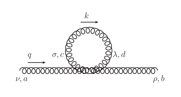
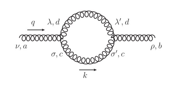
Figure 2: The two diagrams contributing to the vacuum polarization tensor at one loop in the pure glue sector.

4.1 Gluon vacuum polarization tensor at NLO in light-cone gauge

4.1.1 Tadpole diagram

The tadpole diagram (on the left of Fig. 2) might a priori contribute to the gluon vacuum polarization tensor. It writes

$$i\Pi_{\rho\nu}^{ba}(q)\bigg{|}_{\textrm{tad.}}= \,\frac{1}{2}\int\frac{d^{D}k}{(2\pi)^{D}}\;{V_{4g}}_{\nu\rho\sigma\lambda}^{abcd}\;\delta^{cd}\;{\tilde{G}}_{0,F}^{\sigma\lambda}(k)\,,$$ (46)

where the $1/2$ is the symmetry factor associated with the tadpole loop, ${V_{4g}}_{\nu\rho\sigma\lambda}^{abcd}\;$ is the QCD four-gluon vertex, and we use the Feynman propagator in light-cone gauge (3) with the ML pescription (4). Performing the numerator algebra, one arrives at

$$i\Pi_{\rho\nu}^{ba}(q)\bigg{|}_{\textrm{tad.}}= \,\left[{\mathbb{1}}\right]_{ba}\;i\,g^{2}\,C_{A}\,\mu^{4\!-\!D}\int\frac{d^{D}k}{(2\pi)^{D}}\;\frac{i}{\left(k^{2}+i0^{+}\right)}\>\bigg{[}(D\!-\!3)g_{\rho\nu}+\frac{\left(n_{\rho}k_{\nu}+k_{\rho}n_{\nu}\right)}{[n\!\cdot\!k]}\bigg{]}\,\,.$$ (47)

In dimensional regularization, one has the vanishing of the standard scaleless integral

$$\mu^{4\!-\!D}\int\frac{d^{D}k}{(2\pi)^{D}}\;\frac{i}{\left(k^{2}+i0^{+}\right)}= \,0\,,$$ (48)

so that the first term in Eq. (47) vanishes. By contrast, the second term in Eq. (47) involves a vector integral with the denominator $[n\!\cdot\!k]$. Such integral in the ML prescription is a priori a linear combination of the two available vectors $n_{\nu}$ and $\bar{n}_{\nu}$, by Lorentz symmetry. Moreover, integrals with the ML prescription preserve homogeneity with respect to $n_{\nu}$ and with respect to $\bar{n}_{\nu}$. Hence, in this case, the only possible contribution is of the form

$$\mu^{4\!-\!D}\int\frac{d^{D}k}{(2\pi)^{D}}\;\frac{i}{\left(k^{2}+i0^{+}\right)}\;\frac{k_{\nu}}{[n\!\cdot\!k]}= \,C\,\frac{\bar{n}_{\nu}}{\bar{n}\cdot n}\,,$$ (49)

with a constant coefficient $C$. Multiplying the relation (49) with $n^{\nu}$, one finds

$$C= \,n^{\nu}\>\mu^{4\!-\!D}\int\frac{d^{D}k}{(2\pi)^{D}}\;\frac{i}{\left(k^{2}+i0^{+}\right)}\;\frac{k_{\nu}}{[n\!\cdot\!k]}=\mu^{4\!-\!D}\int\frac{d^{D}k}{(2\pi)^{D}}\;\frac{i}{\left(k^{2}+i0^{+}\right)}=0\,,$$ (50)

thanks to Eq. (48). Hence, with the joint use of CDR and the ML prescription, the vector integral appearing in Eq. (47) vanishes identically as well. Hence, the total contribution from the tadpole diagram on the left of Fig. 2 vanishes :

$$i\Pi_{\rho\nu}^{ba}(q)\bigg{|}_{\textrm{tad.}}= \,0\,.$$ (51)

4.1.2 Bubble diagram contribution to the gluon vacuum polarization tensor

The only one-loop contribution to the gluon vacuum polarization tensor is thus the so-called bubble diagram on the right of Fig. 2. Its expression is given by

$$i\Pi_{\rho\nu}^{ba}(q)\bigg{|}_{\textrm{bub.}}= \,\frac{1}{2}\int\frac{d^{D}k}{(2\pi)^{D}}\;{V_{3g}}_{\nu\sigma\lambda}^{acd}(q,-k,k-q)\;{\tilde{G}}_{0,F}^{\sigma^{\prime}\sigma}(k)\,{\tilde{G}}_{0,F}^{\lambda^{\prime}\lambda}(q\!-\!k)\,{V_{3g}}_{\rho\sigma^{\prime}\lambda^{\prime}}^{bcd}(-q,k,q-k)\;$$ (52)

with the standard expression for the 3 gluon vertices in QCD, the symmetry factor $1/2$, and the Feynman propagators taken in the light-cone gauge with the ML prescription (4). The evaluation of the numerator of the integrand requires a significant amount of algebra. The obtained result can be simplified by performing the change of variables $k\mapsto q\!-\!k$ in some of the terms, and use various properties of the encountered integrals. First, we use the Passarino-Veltman reduction relations [61]

$$\mu^{4\!-\!D}\int\frac{d^{D}k}{(2\pi)^{D}}\;\frac{i\;k^{\mu}}{\left(k^{2}+i0^{+}\right)\left((k\!-\!q)^{2}+i0^{+}\right)}= \,\frac{q^{\mu}}{2}\;{\cal B}_{0}(q)$$ (53)

$$\mu^{4\!-\!D}\int\frac{d^{D}k}{(2\pi)^{D}}\;\frac{i\;k^{\mu}k^{\nu}}{\left(k^{2}+i0^{+}\right)\left((k\!-\!q)^{2}+i0^{+}\right)}= \,\frac{1}{(3\!-\!2\epsilon)}\left[\left(1\!-\!\frac{\epsilon}{2}\right)q^{\mu}q^{\nu}-\frac{q^{2}}{4}\,g^{\mu\nu}\right]{\cal B}_{0}(q)$$ (54)

where

$${\cal B}_{0}(q)\equiv \,\mu^{4\!-\!D}\int\frac{d^{D}k}{(2\pi)^{D}}\;\frac{i\;}{\left(k^{2}+i0^{+}\right)\left((k\!-\!q)^{2}+i0^{+}\right)}$$

$$= \,-\frac{1}{(4\pi)^{2}}\,\frac{\Gamma(1\!+\!\epsilon)}{\epsilon}\,\left(\frac{-q^{2}\!-\!i0^{+}}{4\pi\mu^{2}}\right)^{-\epsilon}\,\frac{1}{(1\!-\!2\epsilon)}\,\frac{\Gamma(1\!-\!\epsilon)\Gamma(1\!-\!\epsilon)}{\Gamma(1\!-\!2\epsilon)}\,,$$ (55)

with a UV pole at $\epsilon=0$. Second, we find that

$$\mu^{4\!-\!D}\int\frac{d^{D}k}{(2\pi)^{D}}\;\frac{i}{\left(k^{2}+i0^{+}\right)}\;\frac{1}{[n\!\cdot\!k]}= \,0\,,$$ (56)

in CDR with the ML prescription (4), since in that case both poles in terms of $n\!\cdot\!k$ are always on the same side of the real axis. Finally, one easily finds the relation

$$\mu^{4\!-\!D}\int\frac{d^{D}k}{(2\pi)^{D}}\;\frac{i}{\left((k\!-\!q)^{2}+i0^{+}\right)}\;\frac{1}{[n\!\cdot\!k]}= \,\mu^{4\!-\!D}\int\frac{d^{D}k}{(2\pi)^{D}}\;\frac{i\left(2q\!\cdot\!k\!-\!q^{2}\right)}{\left(k^{2}+i0^{+}\right)\left((k\!-\!q)^{2}+i0^{+}\right)}\;\frac{1}{[n\!\cdot\!k]}\,.$$ (57)

All in all, one finds the expression

$$i\Pi_{\rho\nu}^{ba}(q)\bigg{|}_{\textrm{bub.}}= \,\left[{\mathbb{1}}\right]_{ba}\;i\,g^{2}\,C_{A}\bigg{\{}\Big{[}q_{\rho}q_{\nu}\!-\!q^{2}g_{\rho\nu}\Big{]}\Big{[}\frac{11}{3}+\frac{1}{9}\epsilon+O(\epsilon^{2})\Big{]}{\cal B}_{0}(q)$$

$$\,\;-2(n\!\cdot\!q)\bigg{[}g_{\rho\sigma}\!-\!\frac{n_{\rho}q_{\sigma}}{(n\!\cdot\!q)}\bigg{]}\bigg{[}g_{\mu\nu}\!-\!\frac{q_{\mu}n_{\nu}}{(n\!\cdot\!q)}\bigg{]}\bigg{[}q^{\sigma}\,{\cal I}^{\mu}(q)+q^{\mu}\,{\cal I}^{\sigma}(q)\bigg{]}$$

$$\,\;+4(n\!\cdot\!q)\bigg{[}\left(q_{\rho}\!-\!\frac{q^{2}\,n_{\rho}}{(n\!\cdot\!q)}\right)\left(q_{\nu}\!-\!\frac{q^{2}\,n_{\nu}}{(n\!\cdot\!q)}\right)-\left(q_{\rho}q_{\nu}\!-\!q^{2}g_{\rho\nu}\right)\bigg{]}{\cal I}_{0}(q)\bigg{\}}$$ (58)

with the notations

$${\cal I}_{0}(q)\equiv \,\mu^{4\!-\!D}\int\frac{d^{D}k}{(2\pi)^{D}}\;\frac{i}{\left(k^{2}+i0^{+}\right)\left((k\!-\!q)^{2}+i0^{+}\right)}\;\frac{1}{[n\!\cdot\!k]}$$ (59)

$${\cal I}^{\mu}(q)\equiv \,\mu^{4\!-\!D}\int\frac{d^{D}k}{(2\pi)^{D}}\;\frac{i}{\left(k^{2}+i0^{+}\right)\left((k\!-\!q)^{2}+i0^{+}\right)}\;\frac{k^{\mu}}{[n\!\cdot\!k]}\,.$$ (60)

As a remark, the one-loop contribution (58) is manifestly transverse

$$q^{\rho}i\Pi_{\rho\nu}^{ba}(q)\bigg{|}_{\textrm{bub.}}= \,0\,,$$ (61)

as required from Ward identity [56, 62]. Obviously, one has the relation $n_{\mu}{\cal I}^{\mu}(q)={\cal B}_{0}(q)$. With the ML prescription (4), one can calculate ${\cal I}_{0}(q)$ and the other components of ${\cal I}^{\mu}(q)$, which are finite at $D=4$ and thus will not be needed in the present study. Hence, the vector integral ${\cal I}^{\mu}(q)$ obeys

$${\cal I}^{\mu}(q)= \,\frac{\bar{n}^{\mu}}{\bar{n}\cdot n}\,{\cal B}_{0}(q)+\textrm{finite}+O(\epsilon)\,,$$ (62)

and the UV divergent part of the expression (58) can be isolated as

$$i\Pi_{\rho\nu}^{ba}(q)\bigg{|}_{\textrm{bub.}}= \,\left[{\mathbb{1}}\right]_{ba}\;i\,g^{2}\,C_{A}\bigg{\{}\frac{11}{3}\Big{[}q_{\rho}q_{\nu}\!-\!q^{2}g_{\rho\nu}\Big{]}{\cal B}_{0}(q)-2\frac{(n\!\cdot\!q)}{(\bar{n}\!\cdot\!n)}\bigg{[}q_{\rho}\!-\!\frac{q^{2}\,n_{\rho}}{(n\!\cdot\!q)}\bigg{]}\bigg{[}\bar{n}_{\nu}\!-\!\frac{(\bar{n}\!\cdot\!q)n_{\nu}}{(n\!\cdot\!q)}\bigg{]}{\cal B}_{0}(q)$$

$$\,\;-2\frac{(n\!\cdot\!q)}{(\bar{n}\!\cdot\!n)}\bigg{[}\bar{n}_{\rho}\!-\!\frac{(\bar{n}\!\cdot\!q)n_{\rho}}{(n\!\cdot\!q)}\bigg{]}\bigg{[}q_{\nu}\!-\!\frac{q^{2}\,n_{\nu}}{(n\!\cdot\!q)}\bigg{]}{\cal B}_{0}(q)+\textrm{finite}+O(\epsilon)\bigg{\}}$$ (63)

which is indeed the result found in Ref. [56].

4.1.3 Gluon field renormalization and counterterms

The first UV divergent contribution in Eq. (63) can be compensated by the standard counterterm for gluon field renormalization, which is both local and Lorentz covariant. For example in the $\overline{MS}$ scheme, such counterterm corresponds to a contribution

$$i\Pi_{\rho\nu}^{ba}(q)\bigg{|}_{\textrm{std. c.t.}}= \,\left[{\mathbb{1}}\right]_{ba}\;\frac{i\,g^{2}\,C_{A}}{(4\pi)^{2}}\frac{11}{3}\Big{[}q_{\rho}q_{\nu}\!-\!q^{2}g_{\rho\nu}\Big{]}\bigg{[}\frac{1}{\epsilon}-\gamma_{E}+\log(4\pi)+O(\epsilon)\bigg{]}$$ (64)

to the vacuum polarization tensor.

The other UV divergent terms in Eq. (63) are not Lorentz covariant due to the vectors $n^{\mu}$ and $\bar{n}^{\mu}$, and are non-local. Despite these unusual features, QCD in the light-cone gauge with the ML prescription was shown to be renormalizable in Ref. [62], with a small number of renormalization constant to adjust. Moreover, it was shown in Ref. [62] that only the standard counterterms can contribute to physical observables. We will check in the following that the non-standard UV divergent terms in Eq. (63) drops at the gluon distribution level, so that the corresponding counterterms would drop as well.

4.2 Virtual corrections at the parton distribution level

It remains now to insert the one-loop result (58) for the vacuum polarization tensor into the expression (25) for the virtual correction to the gluon distribution. Noting that, in the target light-cone gauge,

$$n_{\nu}{\tilde{G}}_{0,F}^{\nu i}(q)= \,0$$ (65)

$$q_{\nu}{\tilde{G}}_{0,F}^{\nu i}(q)= \,\frac{i}{[n\!\cdot\!k]}\;n^{i}=0$$ (66)

$$n_{\rho}\,{\cal F}^{-\rho}_{a}= \,{\cal F}^{--}_{a}=0\,,$$ (67)

and that $\partial_{\rho}\,{\cal F}^{-\rho}_{a}$ vanishes up to higher order terms in the coupling $g$, due to the equation of motion of the background field, one finds

$$G(x,\mu^{2})\bigg{|}_{\rm virtual;\,ampl.}^{\rm NLO}= \,\int\frac{d^{D}q}{(2\pi)^{D}}\,\frac{2\pi\delta(q^{-}\!+\!xP^{-})}{(2\pi)xP^{-}}\,\frac{i}{(q^{2}\!+\!i\epsilon)}\>\left[-g^{\nu i}+\frac{n^{\nu}{\mathbf{q}}^{i}}{[n\!\cdot\!q]}\right]\;\int d^{D}\Delta y\,e^{iq\cdot\Delta y}\,\langle P|{\cal F}^{-i}_{a}(0){\cal F}^{-\rho}_{a}(-\Delta y)|P\rangle$$

$$\,\times\;i\,g^{2}\,C_{A}\bigg{\{}-q^{2}g_{\rho\nu}\Big{[}\frac{11}{3}+\frac{1}{9}\epsilon+O(\epsilon^{2})\Big{]}{\cal B}_{0}(q)+4(n\!\cdot\!q)q^{2}g_{\rho\nu}{\cal I}_{0}(q)\bigg{\}}$$

$$= \,g^{2}\,C_{A}\int\frac{d^{D}q}{(2\pi)^{D}}\,\frac{2\pi\delta(q^{-}\!+\!xP^{-})}{(2\pi)xP^{-}}\,\;\int d^{D}\Delta y\,e^{iq\cdot\Delta y}\,\langle P|{\cal F}^{-i}_{a}(0){\cal F}^{-i}_{a}(-\Delta y)|P\rangle$$

$$\,\times\;\bigg{\{}-\Big{[}\frac{11}{3}+\frac{1}{9}\epsilon+O(\epsilon^{2})\Big{]}{\cal B}_{0}(q)+4(n\!\cdot\!q){\cal I}_{0}(q)\bigg{\}}$$ (68)

On the one hand, the $1/\epsilon$ UV pole is subtracted by including the contribution of the $\overline{MS}$ counterterm (64). On the other hand, one can extract the $\mu$ dependence induced by the UV divergence. From the expression (55) of ${\cal B}_{0}(q)$ and the fact that ${\cal I}_{0}(q)$ is UV finite, one gets

$$\mu^{2}\partial_{\mu^{2}}{\cal B}_{0}(q)= \,-\frac{1}{(4\pi)^{2}}\,+O(\epsilon)$$ (69)

$$\mu^{2}\partial_{\mu^{2}}{\cal I}_{0}(q)= \,O(\epsilon)\,,$$ (70)

and thus

$$\mu^{2}\partial_{\mu^{2}}G(x,\mu^{2})\bigg{|}_{\rm virtual;\,ampl.}^{\rm NLO}= \,\frac{11}{3}\,\frac{g^{2}\,C_{A}}{(4\pi)^{2}}\int d^{D}\Delta y\,\langle P|{\cal F}^{-i}_{a}(0){\cal F}^{-i}_{a}(-\Delta y)|P\rangle\int\frac{d^{D}q}{(2\pi)^{D}}\,\frac{2\pi\delta(q^{-}\!+\!xP^{-})}{(2\pi)xP^{-}}\,\,e^{iq\cdot\Delta y}\,+O(\epsilon)$$

$$= \,\frac{11}{3}\,\frac{\alpha_{s}\,C_{A}}{4\pi}\int d\Delta y^{+}\,\frac{e^{-ixP^{-}\Delta y^{+}}}{(2\pi)xP^{-}}\,\langle P|{\cal F}^{-i}_{a}(\Delta y^{+},0:0){\cal F}^{-i}_{a}(0)|P\rangle\;+O(\epsilon)$$

$$= \,\frac{11}{12}\,\frac{\alpha_{s}\,C_{A}}{\pi}\;G^{(0)}(x)+O(\epsilon)$$

$$= \,\frac{11}{12}\,\frac{\alpha_{s}\,C_{A}}{\pi}\;G(x,\mu^{2})+O(\epsilon)+O(\alpha_{s}^{2})\,,$$ (71)

using the relation (22) to trade the bare gluon distribution in favor of the full one, up to higher order contributions in $\alpha_{s}$.

The second diagram on Fig. (1), with the gluon vacuum polarization tensor inserted on the complex conjugate amplitude side would give the same contribution to the DGLAP equation as Eq. (71). All in all, including the contributions the three diagrams from Fig. (1), one finds from Eqs. (45) and (71)

$$\mu^{2}\partial_{\mu^{2}}G(\textrm{x},\mu^{2}) =\frac{\alpha_{s}\,C_{A}}{\pi}\,\int_{\textrm{x}}^{1}\frac{dz}{z}\bigg{[}\frac{z}{(1-z)_{+}}+\frac{(1-z)}{z}+z(1-z)+\frac{11}{6}\,\delta(1-z)\bigg{]}G\left(\frac{{\textrm{x}}}{z},\mu^{2}\right)+O(\alpha_{s}^{2})\,,$$ (72)

which is indeed the well-known LO DGLAP for the gluon distribution in pure Yang-Mills theory. Inclusion of quark effects could be done in the same way. In particular, the gluon Wightman propagator (8) would contribute to the real correction in the quark-to-quark channel, and provide the appropriate $+$ prescription regulating the would-be $z\rightarrow 1$ divergence.

5 Conclusion

We have derived the DGLAP evolution equation for the gluon distribution function using the background field methods of the Color Glass Condensate formalism. Starting with the operator definition of the gluon distribution function in ”target” light cone gauge ($A^{-}=0$ for a left moving proton) in the presence of a background field the DGLAP evolution is cast as the standard UV renormalization of a composite operator constructed from quantum fields, decomposed into background field and fluctuations around it. One loop corrections generate UV divergences for the transverse components of this operator and are regulated via standard techniques using conventional dimensional regularization in $\overline{MS}$ scheme.

While the results presented here are well-known, there are several aspects of this calculation which will be very useful in the pursuit of a unified framework for QCD evolution. With the method developed in this paper we make the connections between the collinear factorization and the CGC effective theory more clear. Having understood how the scale evolution of gluon distribution function arise in the background field formalism in the target light cone gauge, we will repeat the calculation in the ”projectile” light cone gauge ($A^{+}=0$ for a left moving proton) where CGC formalism is most conveniently applied. This will require to fully take into account the gauge link between the field strength tensors in the UV renormalization of the composite operator in the background field formalism. Moreover, this setup and the methods developed here can also adapted to the case of transverse momentum distribution functions (TMDs). We are planning to study the evolution of the TMDs in the presence of the background fields to further investigate the relation between CGC formalism and TMD framework.

References

- [1] F. Gelis, E. Iancu, J. Jalilian-Marian, R. Venugopalan, The Color Glass Condensate, Ann. Rev. Nucl. Part. Sci. 60 (2010) 463–489. arXiv:1002.0333, doi:10.1146/annurev.nucl.010909.083629.
- [2] J. L. Albacete, C. Marquet, Gluon saturation and initial conditions for relativistic heavy ion collisions, Prog. Part. Nucl. Phys. 76 (2014) 1–42. arXiv:1401.4866, doi:10.1016/j.ppnp.2014.01.004.
- [3] J.-P. Blaizot, High gluon densities in heavy ion collisions, Rept. Prog. Phys. 80 (3) (2017) 032301. arXiv:1607.04448, doi:10.1088/1361-6633/aa5435.
- [4] J. Jalilian-Marian, Elastic scattering of a quark from a color field: longitudinal momentum exchange, Phys. Rev. D 96 (7) (2017) 074020. arXiv:1708.07533, doi:10.1103/PhysRevD.96.074020.
- [5] J. Jalilian-Marian, Quark jets scattering from a gluon field: from saturation to high , Phys. Rev. D 99 (1) (2019) 014043. arXiv:1809.04625, doi:10.1103/PhysRevD.99.014043.
- [6] J. Jalilian-Marian, Rapidity loss, spin, and angular asymmetries in the scattering of a quark from the color field of a proton or nucleus, Phys. Rev. D 102 (1) (2020) 014008. arXiv:1912.08878, doi:10.1103/PhysRevD.102.014008.
- [7] V. N. Gribov, L. N. Lipatov, Deep inelastic e p scattering in perturbation theory, Sov. J. Nucl. Phys. 15 (1972) 438–450.
- [8] G. Altarelli, G. Parisi, Asymptotic Freedom in Parton Language, Nucl. Phys. B126 (1977) 298.
- [9] Y. L. Dokshitzer, Calculation of the Structure Functions for Deep Inelastic Scattering and e+ e- Annihilation by Perturbation Theory in Quantum Chromodynamics. (In Russian), Sov. Phys. JETP 46 (1977) 641–653.
- [10] J. Jalilian-Marian, A. Kovner, A. Leonidov, H. Weigert, The BFKL equation from the Wilson renormalization group, Nucl. Phys. B 504 (1997) 415–431. arXiv:hep-ph/9701284, doi:10.1016/S0550-3213(97)00440-9.
- [11] J. Jalilian-Marian, A. Kovner, A. Leonidov, H. Weigert, The Wilson renormalization group for low x physics: Towards the high density regime, Phys. Rev. D 59 (1998) 014014. arXiv:hep-ph/9706377, doi:10.1103/PhysRevD.59.014014.
- [12] J. Jalilian-Marian, A. Kovner, H. Weigert, The Wilson renormalization group for low x physics: Gluon evolution at finite parton density, Phys. Rev. D 59 (1998) 014015. arXiv:hep-ph/9709432, doi:10.1103/PhysRevD.59.014015.
- [13] A. Kovner, J. G. Milhano, Vector potential versus color charge density in low x evolution, Phys. Rev. D 61 (2000) 014012. arXiv:hep-ph/9904420, doi:10.1103/PhysRevD.61.014012.
- [14] A. Kovner, J. G. Milhano, H. Weigert, Relating different approaches to nonlinear QCD evolution at finite gluon density, Phys. Rev. D 62 (2000) 114005. arXiv:hep-ph/0004014, doi:10.1103/PhysRevD.62.114005.
- [15] H. Weigert, Unitarity at small Bjorken x, Nucl. Phys. A 703 (2002) 823–860. arXiv:hep-ph/0004044, doi:10.1016/S0375-9474(01)01668-2.
- [16] E. Iancu, A. Leonidov, L. D. McLerran, Nonlinear gluon evolution in the color glass condensate. 1., Nucl. Phys. A 692 (2001) 583–645. arXiv:hep-ph/0011241, doi:10.1016/S0375-9474(01)00642-X.
- [17] E. Ferreiro, E. Iancu, A. Leonidov, L. McLerran, Nonlinear gluon evolution in the color glass condensate. 2., Nucl. Phys. A 703 (2002) 489–538. arXiv:hep-ph/0109115, doi:10.1016/S0375-9474(01)01329-X.
- [18] T. Altinoluk, N. Armesto, G. Beuf, M. Martínez, C. A. Salgado, Next-to-eikonal corrections in the CGC: gluon production and spin asymmetries in pA collisions, JHEP 07 (2014) 068. arXiv:1404.2219, doi:10.1007/JHEP07(2014)068.
- [19] T. Altinoluk, N. Armesto, G. Beuf, A. Moscoso, Next-to-next-to-eikonal corrections in the CGC, JHEP 01 (2016) 114. arXiv:1505.01400, doi:10.1007/JHEP01(2016)114.
- [20] T. Altinoluk, A. Dumitru, Particle production in high-energy collisions beyond the shockwave limit, Phys. Rev. D 94 (7) (2016) 074032. arXiv:1512.00279, doi:10.1103/PhysRevD.94.074032.
- [21] P. Agostini, T. Altinoluk, N. Armesto, Non-eikonal corrections to multi-particle production in the Color Glass Condensate, Eur. Phys. J. C 79 (7) (2019) 600. arXiv:1902.04483, doi:10.1140/epjc/s10052-019-7097-5.
- [22] P. Agostini, T. Altinoluk, N. Armesto, Effect of non-eikonal corrections on azimuthal asymmetries in the Color Glass Condensate, Eur. Phys. J. C 79 (9) (2019) 790. arXiv:1907.03668, doi:10.1140/epjc/s10052-019-7315-1.
- [23] P. Agostini, T. Altinoluk, N. Armesto, F. Dominguez, J. G. Milhano, Multiparticle production in proton–nucleus collisions beyond eikonal accuracy, Eur. Phys. J. C 82 (11) (2022) 1001. arXiv:2207.10472, doi:10.1140/epjc/s10052-022-10962-1.
- [24] P. Agostini, T. Altinoluk, N. Armesto, Finite width effects on the azimuthal asymmetry in proton-nucleus collisions in the Color Glass Condensate, Phys. Lett. B 840 (2023) 137892. arXiv:2212.03633, doi:10.1016/j.physletb.2023.137892.
- [25] T. Altinoluk, G. Beuf, A. Czajka, A. Tymowska, Quarks at next-to-eikonal accuracy in the CGC: Forward quark-nucleus scattering, Phys. Rev. D 104 (1) (2021) 014019. arXiv:2012.03886, doi:10.1103/PhysRevD.104.014019.
- [26] T. Altinoluk, G. Beuf, Quark and scalar propagators at next-to-eikonal accuracy in the CGC through a dynamical background gluon field, Phys. Rev. D 105 (7) (2022) 074026. arXiv:2109.01620, doi:10.1103/PhysRevD.105.074026.
- [27] T. Altinoluk, G. Beuf, A. Czajka, A. Tymowska, DIS dijet production at next-to-eikonal accuracy in the CGC, Phys. Rev. D 107 (7) (2023) 074016. arXiv:2212.10484, doi:10.1103/PhysRevD.107.074016.
- [28] T. Altinoluk, N. Armesto, G. Beuf, Probing quark transverse momentum distributions in the Color Glass Condensate: quark-gluon dijets in Deep Inelastic Scattering at next-to-eikonal accuracy (3 2023). arXiv:2303.12691.
- [29] Y. V. Kovchegov, D. Pitonyak, M. D. Sievert, Helicity Evolution at Small-x, JHEP 01 (2016) 072, [Erratum: JHEP 10, 148 (2016)]. arXiv:1511.06737, doi:10.1007/JHEP01(2016)072.
- [30] Y. V. Kovchegov, D. Pitonyak, M. D. Sievert, Helicity Evolution at Small : Flavor Singlet and Non-Singlet Observables, Phys. Rev. D 95 (1) (2017) 014033. arXiv:1610.06197, doi:10.1103/PhysRevD.95.014033.
- [31] Y. V. Kovchegov, D. Pitonyak, M. D. Sievert, Small- asymptotics of the quark helicity distribution, Phys. Rev. Lett. 118 (5) (2017) 052001. arXiv:1610.06188, doi:10.1103/PhysRevLett.118.052001.
- [32] Y. V. Kovchegov, D. Pitonyak, M. D. Sievert, Small- Asymptotics of the Quark Helicity Distribution: Analytic Results, Phys. Lett. B 772 (2017) 136–140. arXiv:1703.05809, doi:10.1016/j.physletb.2017.06.032.
- [33] Y. V. Kovchegov, D. Pitonyak, M. D. Sievert, Small- Asymptotics of the Gluon Helicity Distribution, JHEP 10 (2017) 198. arXiv:1706.04236, doi:10.1007/JHEP10(2017)198.
- [34] Y. V. Kovchegov, M. D. Sievert, Small- Helicity Evolution: an Operator Treatment, Phys. Rev. D 99 (5) (2019) 054032. arXiv:1808.09010, doi:10.1103/PhysRevD.99.054032.
- [35] Y. V. Kovchegov, M. D. Sievert, Valence Quark Transversity at Small , Phys. Rev. D 99 (5) (2019) 054033. arXiv:1808.10354, doi:10.1103/PhysRevD.99.054033.
- [36] F. Cougoulic, Y. V. Kovchegov, Helicity-dependent generalization of the JIMWLK evolution, Phys. Rev. D 100 (11) (2019) 114020. arXiv:1910.04268, doi:10.1103/PhysRevD.100.114020.
- [37] Y. V. Kovchegov, Y. Tawabutr, Helicity at Small : Oscillations Generated by Bringing Back the Quarks, JHEP 08 (2020) 014. arXiv:2005.07285, doi:10.1007/JHEP08(2020)014.
- [38] F. Cougoulic, Y. V. Kovchegov, Helicity-dependent extension of the McLerran–Venugopalan model, Nucl. Phys. A 1004 (2020) 122051. arXiv:2005.14688, doi:10.1016/j.nuclphysa.2020.122051.
- [39] D. Adamiak, Y. V. Kovchegov, W. Melnitchouk, D. Pitonyak, N. Sato, M. D. Sievert, First analysis of world polarized DIS data with small-x helicity evolution, Phys. Rev. D 104 (3) (2021) L031501. arXiv:2102.06159, doi:10.1103/PhysRevD.104.L031501.
- [40] Y. V. Kovchegov, A. Tarasov, Y. Tawabutr, Helicity evolution at small x: the single-logarithmic contribution, JHEP 03 (2022) 184. arXiv:2104.11765, doi:10.1007/JHEP03(2022)184.
- [41] Y. V. Kovchegov, M. G. Santiago, Quark sivers function at small : spin-dependent odderon and the sub-eikonal evolution, JHEP 11 (2021) 200, [Erratum: JHEP 09, 186 (2022)]. arXiv:2108.03667, doi:10.1007/JHEP11(2021)200.
- [42] F. Cougoulic, Y. V. Kovchegov, A. Tarasov, Y. Tawabutr, Quark and gluon helicity evolution at small x: revised and updated, JHEP 07 (2022) 095. arXiv:2204.11898, doi:10.1007/JHEP07(2022)095.
- [43] Y. V. Kovchegov, M. G. Santiago, T-odd leading-twist quark TMDs at small x, JHEP 11 (2022) 098. arXiv:2209.03538, doi:10.1007/JHEP11(2022)098.
- [44] J. Borden, Y. V. Kovchegov, Analytic Solution for the Revised Helicity Evolution at Small and Large : New Resummed Gluon-Gluon Polarized Anomalous Dimension and Intercept (4 2023). arXiv:2304.06161.
- [45] G. A. Chirilli, Sub-eikonal corrections to scattering amplitudes at high energy, JHEP 01 (2019) 118. arXiv:1807.11435, doi:10.1007/JHEP01(2019)118.
- [46] G. A. Chirilli, High-energy operator product expansion at sub-eikonal level, JHEP 06 (2021) 096. arXiv:2101.12744, doi:10.1007/JHEP06(2021)096.
- [47] I. Balitsky, A. Tarasov, Rapidity evolution of gluon TMD from low to moderate x, JHEP 10 (2015) 017. arXiv:1505.02151, doi:10.1007/JHEP10(2015)017.
- [48] I. Balitsky, A. Tarasov, Gluon TMD in particle production from low to moderate x, JHEP 06 (2016) 164. arXiv:1603.06548, doi:10.1007/JHEP06(2016)164.
- [49] I. Balitsky, A. Tarasov, Higher-twist corrections to gluon TMD factorization, JHEP 07 (2017) 095. arXiv:1706.01415, doi:10.1007/JHEP07(2017)095.
- [50] I. Balitsky, A. Tarasov, Power corrections to TMD factorization for Z-boson production, JHEP 05 (2018) 150. arXiv:1712.09389, doi:10.1007/JHEP05(2018)150.
- [51] R. Boussarie, Y. Mehtar-Tani, A novel formulation of the unintegrated gluon distribution for DIS, Phys. Lett. B 831 (2022) 137125. arXiv:2006.14569, doi:10.1016/j.physletb.2022.137125.
- [52] R. Boussarie, Y. Mehtar-Tani, Gluon-mediated inclusive Deep Inelastic Scattering from Regge to Bjorken kinematics, JHEP 07 (2022) 080. arXiv:2112.01412, doi:10.1007/JHEP07(2022)080.
- [53] Y. Hatta, Y. Nakagawa, F. Yuan, Y. Zhao, B. Xiao, Gluon orbital angular momentum at small-, Phys. Rev. D 95 (11) (2017) 114032. arXiv:1612.02445, doi:10.1103/PhysRevD.95.114032.
- [54] R. Boussarie, Y. Hatta, F. Yuan, Proton Spin Structure at Small-, Phys. Lett. B 797 (2019) 134817. arXiv:1904.02693, doi:10.1016/j.physletb.2019.134817.
- [55] S. Mandelstam, Light Cone Superspace and the Ultraviolet Finiteness of the N=4 Model, Nucl. Phys. B 213 (1983) 149–168. doi:10.1016/0550-3213(83)90179-7.
- [56] G. Leibbrandt, The Light Cone Gauge in Yang-Mills Theory, Phys. Rev. D 29 (1984) 1699. doi:10.1103/PhysRevD.29.1699.
- [57] A. Bassetto, M. Dalbosco, I. Lazzizzera, R. Soldati, Yang-Mills Theories in the Light Cone Gauge, Phys. Rev. D 31 (1985) 2012. doi:10.1103/PhysRevD.31.2012.
- [58] G. Curci, W. Furmanski, R. Petronzio, Evolution of Parton Densities Beyond Leading Order: The Nonsinglet Case, Nucl. Phys. B 175 (1980) 27–92. doi:10.1016/0550-3213(80)90003-6.
- [59] R. Bufalo, B. M. Pimentel, D. E. Soto, The Epstein-Glaser causal approach to the Light-Front QED4. I: Free theory, Annals Phys. 351 (2014) 1034–1061. arXiv:1405.1896, doi:10.1016/j.aop.2014.08.004.
- [60] A. Bassetto, G. Heinrich, Z. Kunszt, W. Vogelsang, The Light cone gauge and the calculation of the two loop splitting functions, Phys. Rev. D 58 (1998) 094020. arXiv:hep-ph/9805283, doi:10.1103/PhysRevD.58.094020.
- [61] G. Passarino, M. J. G. Veltman, One Loop Corrections for e+ e- Annihilation Into mu+ mu- in the Weinberg Model, Nucl. Phys. B 160 (1979) 151–207. doi:10.1016/0550-3213(79)90234-7.
- [62] A. Bassetto, M. Dalbosco, R. Soldati, Renormalization of the Yang-Mills Theories in the Light Cone Gauge, Phys. Rev. D 36 (1987) 3138. doi:10.1103/PhysRevD.36.3138.