Active matter under control: Insights from response theory

Abstract

Active constituents burn fuel to sustain individual motion, giving rise to collective effects that are not seen in systems at thermal equilibrium, such as phase separation with purely repulsive interactions. There is a great potential in harnessing the striking phenomenology of active matter to build novel controllable and responsive materials that surpass passive ones. Yet, we currently lack a systematic roadmap to predict the protocols driving active systems between different states in a way that is thermodynamically optimal. Equilibrium thermodynamics is an inadequate foundation to this end, due to the dissipation rate arising from the constant fuel consumption in active matter. Here, we derive and implement a versatile framework for the thermodynamic control of active matter. Combining recent developments in stochastic thermodynamics and response theory, our approach shows how to find the optimal control for either continuous- or discrete-state active systems operating out-of-equilibrium. Our results open the door to designing novel active materials which are not only built to stabilize specific nonequilibrium collective states, but are also optimized to switch between different states at minimum dissipation.

I Introduction

Active matter is the class of nonequilibrium systems where individual constituents constantly consume energy to sustain directed motion Marchetti et al. (2013); Gompper et al. (2020); Fodor et al. (2022); O’Byrne et al. (2022). It encompasses both living Prost et al. (2015); Needleman and Dogic (2017) and synthetic systems Paxton et al. (2004); Howse et al. (2007); Palacci et al. (2013); Zöttl and Stark (2016); Vutukuri et al. (2020), which can exhibit emergent phenomena not found at thermal equilibrium. Such emergent –collective– properties are plentiful, ranging from the flocking of animals Toner et al. (2005); Ballerini et al. (2008); Katz et al. (2011), active turbulence Alert et al. (2022), swarming bacteria Darnton et al. (2010); Be’er and Ariel (2019), to motility-induced phase separation (MIPS) that occurs in the absence of attractive particle interactions Cates and Tailleur (2015).

Whilst the collective effects of active matter have been studied extensively, how to efficiently control active matter has only recently started to receive growing attention. Indeed, experiments have now demonstrated the ability to manipulate active nematics with a magnetic field Guillamat et al. (2016), trigger spatial phase separation in bacteria Fragkopoulos et al. (2020), guide rotational patterns in magnetic rotors Matsunaga et al. (2019), and drive phase transitions in living cells Shin et al. (2017). Moreover, the interplay of external control and activity has shown to induce interesting nonlinear behaviours, such as negative mobility, where optimal protocols could result in novel collective functions Rizkallah et al. (2023). Thus, the control of active matter opens unprecedented perspectives on developing novel nonequilibrium materials which selectively change collective states in response to perturbations. To this end, a first step is to establish generic principles for the reliable and optimal control of active systems.

Previous studies have explored the optimal control of active systems through the lens of minimal models. Such works have considered wet one-body control Nasouri et al. (2021); Daddi-Moussa-Ider et al. (2021a, b), one-body navigation strategies Schneider and Stark (2019); Liebchen and Löwen (2019); Piro et al. (2021); Daddi-Moussa-Ider et al. (2021a); Zanovello et al. (2021), and more complex many-body scenarios and field theories Norton et al. (2020); Chennakesavalu and Rotskoff (2021); Cavagna et al. (2022); Falk et al. (2021); Shankar et al. (2022). In these works, optimality typically involves penalizing protocols that steer away from the target state and/or rewards those finishing in the least time, without any constraint on how much energy is dissipated. Therefore, how to optimize control under thermodynamic constraints, such as minimizing the dissipated heat, is still largely unexplored for active systems.

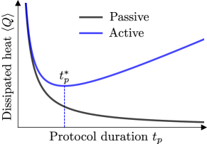
Figure 1: Illustration of the heat dissipated for a control protocol with external perturbation in finite time. In passive systems, the protocol achieving the least dissipation is always the slowest one, as expected from standard thermodynamics. In active systems, the optimal protocol has instead a finite duration $t_{p}^{*}$ which achieves the best trade-off between the dissipation stemming from the external perturbation, and that coming from internal activity.

For passive systems, recent advances in stochastic thermodynamics have led to a versatile framework for control at minimum dissipation Crooks (2007); Sivak and Crooks (2012); Rotskoff and Crooks (2015); Rotskoff et al. (2017); Tafoya et al. (2019); Blaber and Sivak (2020); Deffner and Bonança (2020). In this context, the operator controls the parameters of a given potential energy. The corresponding dissipation decreases with protocol time [Fig. 1], so that the slowest protocol is always optimal, as expected from the thermodynamics of passive systems. For passive systems, the control framework amounts to geometric optimization Crooks (2007); Deffner and Bonança (2020): optimal trajectories are geodesics on curved manifolds of a thermodynamic metric. The success of this geometric approach Rotskoff and Crooks (2015); Rotskoff et al. (2017); Blaber and Sivak (2020); Large and Sivak (2019); Frim and DeWeese (2022) fosters the hope that the underlying framework could also inform control beyond inherently passive systems. How such a framework can be adapted to active matter remains to be explored.

Underpinning the geometric approach for optimal control is linear response theory. It allows one to predict the effect of a weak perturbation in terms of correlations in the unperturbed dynamics. For passive systems, the relation between response and correlation functions follows the celebrated fluctuation-dissipation theorem Kubo (1966), which relies on the time-reversal symmetry (TRS) of the dynamics. Interestingly, such a relation can be straightforwardly extended when TRS is broken Marconi et al. (2008); Baiesi et al. (2009). Indeed, it has already been used to study the response of various active systems Cengio et al. (2019); Maes (2020a); Martin et al. (2021); Cengio et al. (2021); Caprini et al. (2021). These recent developments establish a clear roadmap to extend the framework of thermodynamic control from passive to active systems.

In active systems, the energy consumption of individual constituents results in a constant rate of heat dissipation. Then, in contrast with the control of passive systems, dissipation now stems from two sources: (i) the perturbation by an external operator, and (ii) the internal energy consumption of particles. For a sufficiently large protocol duration, where the dissipation from the perturbation is small, the contribution from internal activity is ever-growing. For a sufficiently small protocol duration, the fast protocol incurs a large dissipation from the large perturbation, as with passive systems. As a result, slow protocols are no longer optimal for the active case, and, now, a finite protocol duration minimizes the dissipation [Fig. 1]. Therefore, the control of active systems involves not only finding optimal trajectories at fixed duration, but also finding which duration achieves the best trade-off between internal and external dissipation. An important challenge is then to rationalize how the optimal duration depends on the interplay between the external perturbation and the internal drive.

In this paper, inspired by previous efforts on passive systems, we herein utilize stochastic thermodynamics and response theory to systematically derive an optimal thermodynamic control framework for active systems. In so doing we build upon recent developments in and applications of linear response theory for active systems Cengio et al. (2019); Maes (2020a); Martin et al. (2021); Cengio et al. (2021); Caprini et al. (2021) and nonlinear response theory for driven thermal systems Lippiello et al. (2008a, b); Basu and Maes (2015); Helden et al. (2016); Basu et al. (2018); Holsten and Krüger (2021). First, we present, in Sec. II, our theoretical framework for the control of both continuous and discrete-state active systems. Second, we show, in Sec. III, how our framework can be deployed to inform the control of some specific model systems. We consider two cases: (i) an active Ornstein-Uhlenbeck particle confined in a harmonic trap with varying stiffness, and (ii) an assembly of active Brownian particles with purely repulsive interactions whose size is varied. In both cases, we obtain the optimal protocol for the corresponding control parameter, and we discuss shared implications that the presence of self-propulsion has on deriving the optimal protocols. Overall, our results provide a systematic framework to address the control of active systems, and illustrate the main differences with respect to the control of passive systems.

II Optimal control

We propose a systematic recipe for optimizing the control of active systems. It consists in predicting how an external operator should vary the parameters of the potential energy to drive the system between two states at minimal cost. We consider the cost function to be the heat dissipated by the system to a thermal reservoir. Assuming weak and slow driving, we decompose the heat into specific correlations and averages, whose dependence on the control parameter determines the optimal protocol. Interestingly, the heat always features a minimum at the protocol time which achieves the best trade-off between internal and external dissipation [Fig. 1].

II.1 Thermodynamic cost function

We consider a system of active particles immersed in a thermal bath at temperature $T$, where each particle $i=\{1,\ldots,N\}$ has an independent self-propulsion velocity $\mathbf{v}_{i}$ that does not depend on position nor on any details of the protocol. We describe the motion of particles by an overdamped Langevin equation given as

$$\dot{\mathbf{r}}_{i}=\mu{\bf f}_{i}+\sqrt{2D}\boldsymbol{\eta}_{i},\quad{\bf f}_{i}=-\nabla_{i}\phi(\alpha,\{\mathbf{r}\})+\mathbf{v}_{i}/\mu,$$ (1)

where $\mathbf{r}_{i}$ is the position of particle $i$, $\mu$ is the mobility, $\phi(\alpha,\{\mathbf{r}\})$ is the total potential energy that depends on the control parameter $\alpha$ and the set of all particle positions $\{\mathbf{r}\}$, $D=\mu T$ is the diffusion coefficient (with Boltzmann constant $k_{\text{B}}=1$), and $\boldsymbol{\eta}_{i}$ is a Gaussian white noise with zero mean and unit variance. The potential energy can account for both particle interactions and external fields. In all what follows, the protocol consists in varying $\alpha(t)$ from its initial value $\alpha_{0}=\alpha(t=0)$ to its final value $\alpha_{1}=\alpha(t=t_{p})$ within the duration $t_{p}$.

For our control problem, we choose the cost function to be the average heat dissipated into the thermal bath (held at temperature $T$) Sekimoto (1998); Seifert (2012); Tociu et al. (2019); Dabelow et al. (2019); Étienne Fodor et al. (2020), defined as

$$\langle Q\rangle=\frac{1}{\mu}\int_{0}^{t_{p}}dt\left\langle\dot{\mathbf{r}}_{i}\cdot\left(\dot{\mathbf{r}}_{i}-\sqrt{2D}\boldsymbol{\eta}_{i}\right)\right\rangle,$$ (2)

where, unless stated otherwise, we perform a sum over repeated indices throughout this paper. Hereafter, the dot product ($\cdot$) is interpreted within Stratonovich convention, for which standard rules of differential calculus carry over to stochastic variables Gardiner (2009). Substituting the dynamics from Eq. (1) into Eq. (2), and using the chain rule $\dot{\mathbf{r}}_{i}\cdot\nabla_{i}\phi=\dot{\phi}-\dot{\alpha}\partial_{\alpha}\phi$, we obtain

$$\langle Q\rangle=\langle\phi_{0}\rangle_{\text{s}}-\langle\phi_{1}\rangle+\int_{0}^{t_{p}}dt\Big{[}\dot{\alpha}\left\langle\partial_{\alpha}\phi\right\rangle+\langle J\rangle\Big{]},$$ (3)

where $\langle X\rangle_{\text{s}}$ denotes the steady-state average of observable $X$, $\phi_{0}$ and $\phi_{1}$ are the initial and final potential energies respectively, and

$$J={\bf f}_{i}\cdot{\bf v}_{i}.$$ (4)

We have assumed that the system is in a steady state at $t=0$, yet it need not be the case at $t=t_{p}$. Equation (3) can be regarded as the extension of the first law of thermodynamics (namely, the conservation of energy) for active systems Fodor and Cates (2021); Fodor et al. (2022). In addition to the potential change $\langle\phi_{0}\rangle_{\text{s}}-\langle\phi_{1}\rangle$ and the work rate $\dot{\alpha}\left\langle\partial_{\alpha}\phi\right\rangle$, that are also present for passive systems, the heat features the dissipation rate $J$. In the passive limit (${\bf v}_{i}={\bm{0}}$ for all $i$) $J$ vanishes, and one recovers the first law of thermodynamics in its standard form.

The self-propulsion term ${\bf v}_{i}/\mu$ in Eq. (1) describes the force on particle $i$ that results from the conversion of energy into directed motion. In active systems such a conversion involves multiple degrees of freedom, deliberately discarded in our framework, that typically provide additional contributions to the heat. Other models of active matter have been proposed which resolve these underlying nonequilibrium processes Pietzonka and Seifert (2017); Speck (2018); Gaspard and Kapral (2019, 2020); Speck (2022). Interestingly, for the case where the chemical reactions between fuel molecules are always transduced into the motion of the active particle, any extra dissipation due to the presence of chemical reactions is only a background contribution, independent of the potential $\phi$. Therefore, all the relevant contributions to the heat arising from $\phi$ are already accounted for in Eq. (3).

In the absence of external control ($\dot{\alpha}=0$), the heat reduces to the last term in Eq. (3), which scales linearly with time: $\langle Q\rangle=\langle J\rangle_{\text{s}}t_{p}$. Such a scaling illustrates that an active system, even when at rest, dissipates heat at a constant rate in order to sustain the self-propulsion of the particles. For a quasi-static protocol, namely for protocol durations much greater than the slowest relaxation timescale of the system ($t_{p}\gg\tau_{\text{max}}$), $\alpha$ will change more slowly than any relaxation timescale of the system. Thus, the system goes through a series of steady states, so that all averages in Eq. (3) are now steady state averages:

$$\langle Q\rangle\underset{t_{p}\gg\tau_{\text{max}}}{=}\langle\phi_{0}\rangle_{\text{s}}-\langle\phi_{1}\rangle_{\text{s}}+\int_{\alpha_{0}}^{\alpha_{1}}\langle\partial_{\alpha}\phi\rangle_{\text{s}}d\alpha+\langle J\rangle_{\text{s}}t_{p}.$$ (5)

At large times, the heat scales linearly with protocol duration [Fig. 1].

We are interested in describing corrections to the quasi-static heat that permit the prediction of optimal control protocols. To this end, we focus on cases where $\alpha$ varies weakly and slowly throughout the protocol. Thus, we can then express the average of a given observable $\langle X\rangle$ in terms of the linear ($R_{1}$) and second-order ($R_{2}$) response functions as

$$\langle X(t)\rangle =\langle X\rangle_{\text{s}}+\int_{-\infty}^{t}dt^{\prime}\Delta\alpha_{t,t^{\prime}}R_{1}(X;t,t^{\prime})$$ (6)

$$\quad+\int_{-\infty}^{t}dt^{\prime}\int_{-\infty}^{t^{\prime}}dt^{\prime\prime}\Delta\alpha_{t,t^{\prime}}\Delta\alpha_{t,t^{\prime\prime}}R_{2}(X;t,t^{\prime},t^{\prime\prime})$$

$$\quad+{\cal O}(\Delta\alpha^{3}),$$

with the time ordering $t\geq t^{\prime}\geq t^{\prime\prime}$, and where $\Delta\alpha_{t,t^{\prime}}\equiv\alpha(t)-\alpha(t^{\prime})$ is the external perturbation to the control parameter. The response functions will be explicitly defined later in Eq. (18). We then expand the perturbation as

$$\Delta\alpha_{t,t^{\prime}}=\dot{\alpha}(t)\Delta t+\frac{{\Delta t}^{2}}{2}\ddot{\alpha}(t)+{\cal O}({\Delta t}^{3}),$$ (7)

where $\Delta t=t-t^{\prime}$ is the time increment. The expansions in Eqs. (6-7) are inspired by a previous work on the control of passive systems Sivak and Crooks (2012), although, here, we expand to higher order in both $\Delta\alpha$ and $\Delta t$. In all what follows, we assume that these expansions are valid at all times within the protocol duration. It amounts to neglecting any abrupt change in the trajectory of $\alpha$, and also regarding the averages in Eq. (3) as smooth functions of time $t$.

Within this setting, we show in Appendix A that the heat can be cast as

$$\langle Q\rangle=B(\alpha_{0},\alpha_{1},\dot{\alpha}_{0},\dot{\alpha}_{1})+\int_{0}^{t_{p}}dt\mathcal{L}(\dot{\alpha},\alpha),$$ (8)

where $\dot{\alpha}_{0}=\dot{\alpha}(t=0)$ and $\dot{\alpha}_{1}=\dot{\alpha}(t=t_{p})$, and we have introduced the boundary term

$$B =\langle\phi_{0}\rangle_{\text{s}}-\langle\phi_{1}\rangle_{\text{s}}+\dot{\alpha}_{0}\Sigma(\alpha_{0})-\dot{\alpha}_{1}(\Phi+\Sigma)(\alpha_{1})$$ (9)

$$\quad+\int_{\alpha_{0}}^{\alpha_{1}}d\alpha\Lambda(\alpha),$$

and the Lagrangian

$$\mathcal{L}(\dot{\alpha},\alpha)=\dot{\alpha}^{2}(\Psi-\Sigma^{\prime})(\alpha)-V(\alpha),\quad\Sigma^{\prime}=d\Sigma/d\alpha.$$ (10)

The functions $\{V,\Phi,\Sigma,\Lambda,\Psi\}$ are given by

$$V =-\langle J\rangle_{\text{s}},\qquad\Phi=\int_{0}^{\infty}dtR_{1}({\phi};t,0)t,$$ (11)

$$\Sigma =\frac{1}{2}\int_{0}^{\infty}dtR_{1}\left(J;t,0\right)t^{2},$$

$$\Lambda =\langle\partial_{\alpha}\phi\rangle_{\text{s}}+\int_{0}^{\infty}dtR_{1}\left(J;t,0\right)t,$$

$$\Psi =\int_{0}^{\infty}dtR_{1}({\partial_{\alpha}\phi};t,0)t$$

$$\quad+\frac{1}{2}\int_{0}^{\infty}\int_{0}^{\infty}dtdt^{\prime}R_{2}\left(J;t^{\prime},t^{\prime}-t,0\right)tt^{\prime},$$

The decomposition of heat in Eqs. (8-11) is one of the central results of this paper. By measuring response functions and averages at different values of $\alpha$, one can systematically construct the dependence of the Lagrangian $\cal L$ in terms of $\alpha$ and $\dot{\alpha}$, and deduce the expression of the corresponding heat for any protocol. Indeed, experimentally measured linear and nonlinear response functions Molaei et al. (2023) can be injected into Eqs. (8-11) to explicitly determine the functional dependence of the heat on the control parameter. The optimal protocol readily follows from $\cal L$ by straightforward optimization [Sec. II.2]. Importantly, Eqs. (8-11) hold for any potential $\phi$ and self-propulsion ${\bf v}_{i}$, which highlights the versatility of our approach.

In the absence of self-propulsion (${\bf v}_{i}={\bf 0}$), the Lagrangian reduces to ${\cal L}=\dot{\alpha}^{2}\Psi(\alpha)$, in agreement with previous results on controlling passive systems Sivak and Crooks (2012). As detailed in Sec. II.2, the difference in $\cal L$ between active and passive systems drastically affects the corresponding dependence of $\langle Q\rangle$ in terms of $t_{p}$. The heat monotonically decreases in the passive case, whereas it features a global minimum in the active case [Fig. 1]. Therefore, although our approach only accounts for leading-order corrections to the quasistatic regime, it is actually sufficient to capture the main qualitative change between optimizing either passive or active matter.

II.2 Optimal protocol

Our aim is to demonstrate that the heat decomposition in Eqs. (8-11) entails a series of generic properties, both for the optimal protocol $\alpha(t)$ and for the corresponding optimal heat $\langle Q\rangle$. Interestingly, we derive such properties without actually specifying the explicit dependence of the functions $\{V,\Phi,\Sigma,\Lambda,\Psi\}$ on $\alpha$ [Eq. (11)]. For an arbitrary potential $\phi$ and self-propulsion ${\bf v}_{i}$, we then predict how $\langle Q\rangle$ scales with the protocol time $t_{p}$, and we provide an approximate estimation of the value $t_{p}^{*}$ minimizing $\langle Q\rangle$.

Our derivations essentially rely on drawing an analogy between the Lagrangian $\cal L$ in Eq. (10), and that of a harmonic oscillator with position-dependent mass Khlevniuk and Tymchyshyn (2018). In that respect, $V(\alpha)$ and $\dot{\alpha}^{2}(\Psi-\Sigma^{\prime})(\alpha)$ respectively stand for the potential and kinetic energies, where the effective mass $\Psi-\Sigma^{\prime}$ here depends on the control parameter $\alpha$. In what follows, we assume that $V(\alpha)$ is bounded and $(\Psi-\Sigma^{\prime})(\alpha)\geq 0$ for all $\alpha$ between $\alpha_{0}$ and $\alpha_{1}$, which ensures the validity of our analogy. The optimal trajectory then obeys the following Euler-Lagrange equation:

$$2\ddot{\alpha}(\Psi-\Sigma^{\prime})(\alpha)+\dot{\alpha}^{2}(\Psi^{\prime}-\Sigma^{\prime\prime})(\alpha)=-V^{\prime}(\alpha).$$ (12)

As in standard Hamiltonian mechanics, one can also display the optimal trajectory in terms of a first integral of motion. Multiplying both sides of Eq. (12) by $\dot{\alpha}$, and integrating with respect to time $t$, we get

$$E=\dot{\alpha}^{2}(\Psi-\Sigma^{\prime})(\alpha)+V(\alpha).$$ (13)

The term $E$ is analogous to the total energy in Hamiltonian mechanics. It is constant throughout the protocol, and it is constrained by $E>\underset{\alpha}{\max}\,V$.

We deduce from Eq. (13) a relation between the protocol trajectory $\alpha(t)$ and the protocol speed $\dot{\alpha}(t)$:

$$\dot{\alpha}=\pm\sqrt{\frac{E-V(\alpha)}{(\Psi-\Sigma^{\prime})(\alpha)}},$$ (14)

which shows that the optimal trajectory obeys a first-order ordinary differential equation. This differential equation can be solved by separation of variables, and it is fully determined by $\{E,V,\Psi,\Sigma\}$. In practice, the constant of motion $E$ implicitly depends on the initial and final values $\{\alpha_{0},\alpha_{1}\}$, and on the protocol duration $t_{p}$. Indeed, separating variables in Eq. (14), and integrating throughout the protocol, we get

$$t_{p}=\left|\int_{\alpha_{0}}^{\alpha_{1}}d\alpha\sqrt{\frac{(\Psi-\Sigma^{\prime})(\alpha)}{E-V(\alpha)}}\right|.$$ (15)

Therefore, combining Eqs. (14-15), the solution of the optimal trajectory $\alpha(t)$ follows directly. Although its explicit expression cannot be given analytically for generic potential $\phi$ and self-propulsion ${\bf v}_{i}$, numerical integration readily yields $\alpha(t)$ for given expressions of $\{V,\Psi,\Sigma\}$, and for arbitrary $\{\alpha_{0},\alpha_{1}\}$ and $t_{p}$.

Interestingly, we demonstrate in Appendix B that Eqs. (14-15) are actually sufficient to predict how $\langle Q\rangle$ scales with protocol duration $t_{p}$:

$$\langle Q\rangle\underset{t_{p}\ll t_{p}^{*}}{\sim}K(\alpha_{0},\alpha_{1})/t_{p},$$ (16)

$$\langle Q\rangle\underset{t_{p}\gg t_{p}^{*}}{\sim}t_{p}\,\underset{\alpha}{\min}\langle J\rangle_{\text{s}},$$

where the expression of $K(\alpha_{0},\alpha_{1})$ follows from that of $\{\Phi,\Psi,\Sigma\}$ [Eq. (58)]. These scalings correspond to regimes where the dissipation is dominated either by the external driving of the control parameter $\alpha$ (namely for $t_{p}\ll t_{p}^{*}$), or by the internal self-propulsion ${\bf v}_{i}$ (namely for $t_{p}\gg t_{p}^{*}$). The former reproduces the scaling expected for passive systems Sivak and Crooks (2012). The latter agrees with the quasistatic prediction [Eq. (5)], where here the optimal protocol achieves the minimum value of $\langle J\rangle_{s}$, as expected.

In between the regimes of large and small $t_{p}$, the heat reaches a minimum at $t_{p}=t_{p}^{*}$ [Fig. 1]. The protocol duration $t_{p}^{*}$ achieves the best compromise between two regimes of high $\langle Q\rangle$. By extending the scalings in Eq. (16) to regimes where $t_{p}\approx t_{p}^{*}$, we approximate $t_{p}^{*}$ as the value of $t_{p}$ where these scalings have same $\langle Q\rangle$:

$$t_{p}^{\ast}\approx\sqrt{K(\alpha_{0},\alpha_{1})\big{/}\underset{\alpha}{\min}\langle J\rangle_{\text{s}}}.$$ (17)

Equation (17) illustrates that $t_{p}^{*}$ sets a trade-off between (i) the heat due to external drive, involving the system relaxation through response functions in the definition of $K(\alpha_{0},\alpha_{1})$ (equivalently in the definition of $\{\Phi,\Psi,\Sigma\}$, see Eq. (11)), and (ii) the heat due to internal self-propulsion, involving the steady state average $\langle J\rangle_{s}$. A qualitatively similar trade-off was reported in a different context for systems combining autonomous cycles and external drives Bryant and Machta (2020).

In the passive limit (${\bf v}_{i}={\bf 0}$), we deduce from Eq. (17) that $t_{p}^{*}$ diverges. The heat now reaches its minimum asymptotically at large $t_{p}$ [Fig. 1], and the scaling corresponding to $t_{p}\ll t_{p}^{*}$ in Eq. (16) now extends to all $t_{p}$. Indeed, as expected from the thermodynamics of passive systems, the protocol with smallest dissipation is always the slowest, in which case the heat reduces to its quasistatic value.

Interestingly, when controlling active systems, the boundary term $B$ in Eq. (9) involves the protocol speeds $\dot{\alpha}$ at initial and final times, respectively $\dot{\alpha}_{0}$ and $\dot{\alpha}_{1}$. Within our framework, optimizing the Lagragian term $\cal L$ already leads to fixing $\dot{\alpha}_{0}$ and $\dot{\alpha}_{1}$ [Eqs. (14-15)] for a given choice of $\{\alpha_{0},\alpha_{1}\}$ and $t_{p}$. To optimize simultaneously $B$ and $\cal L$, one could potentially consider abrupt changes in the protocol trajectory $\alpha(t)$ at initial and final times Schmiedl and Seifert (2007). Yet, such discontinuous jumps would not be consistent with the expansions in Eqs. (6-7). Therefore, in what follows, we focus on the optimal trajectory given by Eqs. (14-15).

II.3 Response functions

We now demonstrate that the response functions in the heat decomposition of Eqs. (8-11) can be expressed in terms of some specific correlations functions. Indeed, evaluating response functions generally requires measuring how the system is affected by weak perturbation, which can prove difficult both in numerical simulations and in experiments. Instead, our aim is to show that the response is actually already encoded in spontaneous fluctuations of the unperturbed dynamics.

In passive systems, the fluctuation-dissipation theorem enforces generic relations between linear response and correlation functions Kubo (1966), and similar types of relations also exist for the second-order response Basu et al. (2015); Basu and Maes (2015); Helden et al. (2016). Interestingly, recent works have shown that response-correlation relations can be extended beyond passive systems Maes (2020a), and in particular to active matter Cengio et al. (2019); Martin et al. (2021); Cengio et al. (2021); Caprini et al. (2021). Here, we explicitly derive such relations for the active dynamics in Eq. (1).

From the definition of the response functions in Eq. (6) for a generic observable $X$, we express $R_{1}$ and $R_{2}$ as

$$R_{1}(X;t,t^{\prime}) =\frac{\delta\langle X(t)\rangle}{\delta\Delta\alpha_{t,t^{\prime}}}\bigg{|}_{\Delta\alpha\to 0},$$ (18)

$$R_{2}(X;t,t^{\prime},t^{\prime\prime}) =\frac{\delta^{2}\langle X(t)\rangle}{\delta\Delta\alpha_{t,t^{\prime}}\delta\Delta\alpha_{t,t^{\prime\prime}}}\bigg{|}_{\Delta\alpha\to 0}.$$

Evaluating the response functions then amounts to predicting how the average $\langle X(t)\rangle$ is perturbed when varying the control parameter $\alpha$. To this end, we express this average in terms of a path integral as

$$\langle X(t)\rangle =\int X(t)\prod_{i}P_{\eta}[{\bm{\eta}}_{i}]P_{v}[{\bf v}_{i}]{\cal D}{\bm{\eta}}_{i}{\cal D}{\bf v}_{i}$$ (19)

$$\quad\times\delta\big{(}\dot{\bf r}_{i}-\mu{\bf f}_{i}({\bf r}_{i},{\bf v}_{i})+\sqrt{2D}{\bm{\eta}}_{i}\big{)}{\cal D}{\bf r}_{i},$$

where $P_{\eta}$ and $P_{v}$ denote the probabilites to observe a given trajectory for the noise terms ${\bm{\eta}}_{i}$ and ${\bf v}_{i}$, respectively. We have used that these noises are independent. Using that $P_{\eta}$ is Gaussian, integrating Eq. (19) with respect to position trajectories $\{{\bf r}_{i}\}$ yields

$$\langle X(t)\rangle={\cal N}\int X(t)\,e^{-{\cal S}}{\cal D}[{\bm{\eta}},{\bf v}],$$ (20)

where ${\cal D}[{\bm{\eta}},{\bf v}]=\prod_{i}P_{v}[{\bf v}_{i}]{\cal D}{\bm{\eta}}_{i}{\cal D}{\bf v}_{i}$, and the normalization factor is given by $1/{\cal N}=\int e^{-{\cal S}}{\cal D}[{\bm{\eta}},{\bf v}]$. The term $\cal S$ is the standard Onsager-Machlup action Onsager and Machlup (1953):

$$\mathcal{S}=\frac{1}{4D}\int_{0}^{t_{p}}dt\left(\dot{\mathbf{r}}_{i}-\mu\mathbf{f}_{i}\right)^{2}.$$ (21)

Note that, although the dynamics is given in Stratonovich convention throughout the paper, $\cal S$ does not feature the term $(\mu/2)\int dt\nabla_{i}\cdot{\bf f}_{i}$ usually given in the Onsager-Machlup action. This is because the path integral in Eq. (20) is written with respect to noise trajectories, instead of position trajectories.

Substituting the path integral of Eq. (20) into Eq. (18), we deduce

$$R_{1}(X;t,t^{\prime}) =\int X(t)\frac{\delta\big{(}{\cal N}e^{-{\cal S}}\big{)}}{\delta\Delta\alpha_{t,t^{\prime}}}\bigg{|}_{\Delta\alpha\to 0}{\cal D}[{\bm{\eta}},{\bf v}],$$ (22)

$$R_{2}(X;t,t^{\prime},t^{\prime\prime}) =\int X(t)\frac{\delta^{2}\big{(}{\cal N}e^{-{\cal S}}\big{)}}{\delta\Delta\alpha_{t,t^{\prime}}\delta\Delta\alpha_{t,t^{\prime\prime}}}\bigg{|}_{\Delta\alpha\to 0}{\cal D}[{\bm{\eta}},{\bf v}],$$

where we have used that ${\cal D}[{\bm{\eta}},{\bf v}]$ is independent of $\alpha$, since noise trajectories are not affected by the control parameter. Then, predicting how $\cal S$ varies with $\alpha$ is a route to expressing $R_{1}$ and $R_{2}$ in terms of correlation functions. The perturbation $\alpha\to\alpha-\Delta\alpha$ affects the action as $\mathcal{S}\to\mathcal{S}+\Delta\mathcal{S}$, where

$$\Delta\mathcal{S} =\frac{1}{4T}\int_{0}^{t_{p}}dt\Big{[}-2\Delta\alpha(\nabla_{i}\partial_{\alpha}\phi)\cdot\left(\dot{\mathbf{r}}_{i}-\mu\mathbf{f}_{i}\right)$$ (23)

$$\quad+\Delta\alpha^{2}\left(\mu(\nabla_{i}\partial_{\alpha}\phi)^{2}+(\nabla_{i}\partial_{\alpha}^{2}\phi)\cdot(\dot{\mathbf{r}}_{i}-\mu\mathbf{f}_{i})\right)\Big{]}$$

$$\quad+\mathcal{O}(\Delta\alpha^{3}).$$

As detailed in Appendix C.1, combining Eqs. (22-23) then leads to

$$2TR_{1}(X;t,t^{\prime})=\frac{d}{dt^{\prime}}\mathopen{\hbox{\set@color${\big{\langle}}$}\kern-1.94444pt\leavevmode\hbox{\set@color${\big{\langle}}$}}{X}_{t}[\partial_{\alpha}\phi]_{t^{\prime}}\mathclose{\hbox{\set@color${\big{\rangle}}$}\kern-1.94444pt\leavevmode\hbox{\set@color${\big{\rangle}}$}}-\mu\mathopen{\hbox{\set@color${\big{\langle}}$}\kern-1.94444pt\leavevmode\hbox{\set@color${\big{\langle}}$}}X_{t}\big{[}(\nabla_{i}\partial_{\alpha}\phi)\cdot\mathbf{f}_{i}\big{]}_{t^{\prime}}\mathclose{\hbox{\set@color${\big{\rangle}}$}\kern-1.94444pt\leavevmode\hbox{\set@color${\big{\rangle}}$}}.$$ (24)

The connected correlation $\mathopen{\hbox{\set@color${\langle}$}\kern-1.94444pt\leavevmode\hbox{\set@color${\langle}$}}X(t)Y(t^{\prime})\mathclose{\hbox{\set@color${\rangle}$}\kern-1.94444pt\leavevmode\hbox{\set@color${\rangle}$}}\equiv\mathopen{\hbox{\set@color${\langle}$}\kern-1.94444pt\leavevmode\hbox{\set@color${\langle}$}}X_{t}Y_{t^{\prime}}\mathclose{\hbox{\set@color${\rangle}$}\kern-1.94444pt\leavevmode\hbox{\set@color${\rangle}$}}$ is defined for arbitrary observables $X$ and $Y$ as

$$\mathopen{\hbox{\set@color${\langle}$}\kern-1.94444pt\leavevmode\hbox{\set@color${\langle}$}}X_{t}Y_{t^{\prime}}\mathclose{\hbox{\set@color${\rangle}$}\kern-1.94444pt\leavevmode\hbox{\set@color${\rangle}$}}=\langle X_{t}Y_{t^{\prime}}\rangle-\langle X\rangle_{\text{s}}\langle Y\rangle_{\text{s}}.$$ (25)

In the absence of self-propulsion (${\bf v}_{i}={\bf 0}$), we recover the celebrated fluctuation-dissipation theorem: $R_{1}(X;t,t^{\prime})=(1/T)(d/dt^{\prime})\mathopen{\hbox{\set@color${\langle}$}\kern-1.94444pt\leavevmode\hbox{\set@color${\langle}$}}X(t)\partial_{\alpha}\phi(t^{\prime})\mathclose{\hbox{\set@color${\rangle}$}\kern-1.94444pt\leavevmode\hbox{\set@color${\rangle}$}}$ for $t>t^{\prime}$ Kubo (1966). Indeed, this theorem is readily obtained from Eq. (24) by considering the time-symmetrized response $R_{1}(X;t,t^{\prime})-R_{1}(X;t^{\prime},t)$, and using the time-reversal symmetry of equilibrium correlations Maes (2020a) (see Appendix C.1). Similarly, we show in Appendix C.1 that the second-order response can be written as

$$4T^{2}\,R_{2}(X;t,t^{\prime},t^{\prime\prime})$$ (26)

$$=\frac{d}{dt^{\prime}}\frac{d}{dt^{\prime\prime}}\mathopen{\hbox{\set@color${\big{\langle}}$}\kern-1.94444pt\leavevmode\hbox{\set@color${\big{\langle}}$}\kern-1.94444pt\leavevmode\hbox{\set@color${\big{\langle}}$}}{X}_{t}[\partial_{\alpha}\phi]{}_{t^{\prime}}[\partial_{\alpha}\phi]{}_{t^{\prime\prime}}\mathclose{\hbox{\set@color${\big{\rangle}}$}\kern-1.94444pt\leavevmode\hbox{\set@color${\big{\rangle}}$}\kern-1.94444pt\leavevmode\hbox{\set@color${\big{\rangle}}$}}+\mu^{2}\mathopen{\hbox{\set@color${\big{\langle}}$}\kern-1.94444pt\leavevmode\hbox{\set@color${\big{\langle}}$}\kern-1.94444pt\leavevmode\hbox{\set@color${\big{\langle}}$}}{X}_{t}\big{[}(\nabla_{i}\partial_{\alpha}\phi)\cdot\mathbf{f}_{i}\big{]}{}_{t^{\prime}}\big{[}(\nabla_{j}\partial_{\alpha}\phi)\cdot\mathbf{f}_{j}\big{]}{}_{t^{\prime\prime}}\mathclose{\hbox{\set@color${\big{\rangle}}$}\kern-1.94444pt\leavevmode\hbox{\set@color${\big{\rangle}}$}\kern-1.94444pt\leavevmode\hbox{\set@color${\big{\rangle}}$}}-\mu\frac{d}{dt^{\prime\prime}}\mathopen{\hbox{\set@color${\big{\langle}}$}\kern-1.94444pt\leavevmode\hbox{\set@color${\big{\langle}}$}\kern-1.94444pt\leavevmode\hbox{\set@color${\big{\langle}}$}}{X}_{t}[\partial_{\alpha}\phi]{}_{t^{\prime\prime}}\big{[}(\nabla_{i}\partial_{\alpha}\phi)\cdot\mathbf{f}_{i}\big{]}{}_{t^{\prime}}\mathclose{\hbox{\set@color${\big{\rangle}}$}\kern-1.94444pt\leavevmode\hbox{\set@color${\big{\rangle}}$}\kern-1.94444pt\leavevmode\hbox{\set@color${\big{\rangle}}$}}$$

$$\quad-\mu\frac{d}{dt^{\prime}}\mathopen{\hbox{\set@color${\big{\langle}}$}\kern-1.94444pt\leavevmode\hbox{\set@color${\big{\langle}}$}\kern-1.94444pt\leavevmode\hbox{\set@color${\big{\langle}}$}}{X}_{t}[\partial_{\alpha}\phi]{}_{t^{\prime}}\big{[}(\nabla_{i}\partial_{\alpha}\phi)\cdot\mathbf{f}_{i}\big{]}{}_{t^{\prime\prime}}\mathclose{\hbox{\set@color${\big{\rangle}}$}\kern-1.94444pt\leavevmode\hbox{\set@color${\big{\rangle}}$}\kern-1.94444pt\leavevmode\hbox{\set@color${\big{\rangle}}$}}-2T\delta(t^{\prime}-t^{\prime\prime})\bigg{[}\frac{d}{dt^{\prime}}\mathopen{\hbox{\set@color${\big{\langle}}$}\kern-1.94444pt\leavevmode\hbox{\set@color${\big{\langle}}$}}X_{t}[\partial_{\alpha}^{2}\phi]{}_{t^{\prime}}\mathclose{\hbox{\set@color${\big{\rangle}}$}\kern-1.94444pt\leavevmode\hbox{\set@color${\big{\rangle}}$}}+\mu\mathopen{\hbox{\set@color${\big{\langle}}$}\kern-1.94444pt\leavevmode\hbox{\set@color${\big{\langle}}$}}{X}_{t}\big{[}(\nabla_{i}\partial_{\alpha}\phi)^{2}-(\nabla_{i}\partial_{\alpha}^{2}\phi)\cdot\mathbf{f}_{i}\big{]}{}_{t^{\prime}}\mathclose{\hbox{\set@color${\big{\rangle}}$}\kern-1.94444pt\leavevmode\hbox{\set@color${\big{\rangle}}$}}\bigg{]},$$

where the connected correlation $\mathopen{\hbox{\set@color${\langle}$}\kern-1.94444pt\leavevmode\hbox{\set@color${\langle}$}\kern-1.94444pt\leavevmode\hbox{\set@color${\langle}$}}X(t)Y(t^{\prime})Z(t^{\prime\prime})\mathclose{\hbox{\set@color${\rangle}$}\kern-1.94444pt\leavevmode\hbox{\set@color${\rangle}$}\kern-1.94444pt\leavevmode\hbox{\set@color${\rangle}$}}\equiv\mathopen{\hbox{\set@color${\langle}$}\kern-1.94444pt\leavevmode\hbox{\set@color${\langle}$}\kern-1.94444pt\leavevmode\hbox{\set@color${\langle}$}}X_{t}Y_{t^{\prime}}Z_{t^{\prime\prime}}\mathclose{\hbox{\set@color${\rangle}$}\kern-1.94444pt\leavevmode\hbox{\set@color${\rangle}$}\kern-1.94444pt\leavevmode\hbox{\set@color${\rangle}$}}$ is defined for arbitrary observables $X$, $Y$, and $Z$ as

$$\mathopen{\hbox{\set@color${\langle}$}\kern-1.94444pt\leavevmode\hbox{\set@color${\langle}$}\kern-1.94444pt\leavevmode\hbox{\set@color${\langle}$}}X_{t}Y_{t^{\prime}}Z_{t^{\prime\prime}}\mathclose{\hbox{\set@color${\rangle}$}\kern-1.94444pt\leavevmode\hbox{\set@color${\rangle}$}\kern-1.94444pt\leavevmode\hbox{\set@color${\rangle}$}} =\langle X_{t}Y_{t^{\prime}}Z_{t^{\prime\prime}}\rangle-\langle X\rangle_{\text{s}}\langle Y_{t^{\prime}}Z_{t^{\prime\prime}}\rangle$$ (27)

$$\quad-\langle Y\rangle_{\text{s}}\langle X_{t}Z_{t^{\prime\prime}}\rangle-\langle Z\rangle_{\text{s}}\langle X_{t}Y_{t^{\prime}}\rangle$$

$$\quad+2\langle X\rangle_{\text{s}}\langle Y\rangle_{\text{s}}\langle Z\rangle_{\text{s}}.$$

The relations in Eqs. (24-27), coupled with Eqs. (8-11), are the main relations of this paper. Indeed, they provide explicit connections between the response functions $R_{1}$ and $R_{2}$, defined for an arbitrary observable $X$ [Eq. (6)], and correlation functions in the unperturbed dynamics. Similar linear and nonlinear response relations have been previously derived in the context of general Markov and non-equilibrium systems, with specific application to the Langevin equation and Ising spin variables  Lippiello et al. (2008a, b). Our response relations Eqs. (24-27) provide a route to evaluating response functions resulting from external control without actually perturbing the system. Overall, we are now in a position to deploy these relations to the specific observables which define the response functions of interest in Eq. (11).

II.4 Discrete-state dynamics

In this section, we show that our generic framework for controlling the potential in Eq. (1), corresponding to a continuous-state dynamics, can be extended to nonequilibrium systems with discrete states. To this end, we consider a generic dynamics that is governed by the following master equation:

$$\dot{p}_{i}=\sum_{j}K_{ij}(\alpha)\,p_{j},$$ (28)

where $p_{i}(t)$ is the probability for the system to be in the state $i$ at time $t$, and $K_{ij}$ is the transition rate to go from state $j$ to $i$. The control parameter $\alpha$ determines the expression of $K_{ij}$, analogously to how $\alpha$ controls the potential $\phi$ in Eq. (1). The average of a given observable $X$ and its time derivative are expressed as

$$\langle X\rangle =\sum_{i}X_{i}p_{i},$$ (29)

$$\langle\dot{X}\rangle =\sum_{i}\Big{[}p_{i}\dot{\alpha}\partial_{\alpha}X_{i}+X_{i}\sum_{j}K_{ij}p_{j}\Big{]},$$

where $X_{i}$ is the projection of $X$ over the state $i$. As for the continuous-state case, the system is in contact with a heat bath at temperature $T$, and subject to active driving. In practice, we consider transition rates with Arrhenius form, ensuring that the dynamics is thermodynamically consistent Arrhenius (1889); Herpich et al. (2018). Such a transition rate is given by

$$K_{ij}(\alpha)=c_{ij}\exp\left(-\frac{\phi_{j}(\alpha)-\phi_{i}(\alpha)+\varepsilon_{ij}}{2T}\right)$$ (30)

where $c_{ij}=c_{ji}$ is the rate amplitude, $\phi_{i}$ is the potential energy of state $i$, and $\varepsilon_{ij}=-\varepsilon_{ji}$ is the energy exchange associated with the active driving.

The heat dissipated into the bath while varying $\alpha$ from $\alpha_{0}$ to $\alpha_{1}$, within a time duration $t_{p}$, reads Lebowitz and Spohn (1999); den Broeck and Esposito (2015)

$$\langle Q\rangle=T\int_{0}^{t_{p}}dt\sum_{i,j}K_{ij}p_{j}\ln\frac{K_{ij}}{K_{ji}}.$$ (31)

Substituting the definition of the transition rates from Eq. (30) into Eq. (31), we get

$$\langle Q\rangle=\langle\phi(\alpha_{0})\rangle_{\text{s}}-\langle\phi(\alpha_{1})\rangle+\int_{0}^{t_{p}}dt\Big{[}\dot{\alpha}\langle\partial_{\alpha}\phi\rangle+\langle J\rangle\Big{]},$$ (32)

where we have used the definition of averages given in Eq. (29), and we have introduced the active dissipation rate:

$$\langle J\rangle=\sum_{i,j}K_{ij}p_{j}\varepsilon_{ij}.$$ (33)

The first law of thermodynamics in Eq. (32) takes a similar form as for the continuous-state case in Eq. (3). Therefore, within the same set of assumptions as in Sec. II.1, the decomposition of heat as the sum of boundary and Lagrangian term [Eqs. (8-11)] remains valid for the discrete-state case, as with all the results for the optimal protocol in Sec. II.2.

Again, to connect response functions to correlation functions, as for the case of continuous-state dynamics [Sec. II.3], we rely on a path-integral approach. First, we define the path weight of a given trajectory $\omega([0,t_{p}])$ which goes through a series of discrete states within the protocol time $t_{p}$ Seifert (2012); Maes et al. (2008); Maes (2020b):

$$P=\mathcal{N}\exp(-\mathcal{A}),$$ (34)

with the normalization factor $\mathcal{N}$. The action $\cal A$ reads

$$\mathcal{A}=\int_{0}^{t_{p}}dt\sum_{i,j\neq i}\left[(K_{ij}-\bar{K}_{ij})\rho_{j}(t)+n_{ij}(t)\ln\frac{\bar{K}_{ij}}{K_{ij}}\right],$$ (35)

where we have introduced the reference transition rate $\bar{K}_{ij}$ that does not depend on $\alpha$. The stochastic density $\rho_{j}(t)$ is $1$ if the trajectory $\omega([0,t])$ goes through the state $j$ at time $t$, and $0$ otherwise:

$$\rho_{j}(t)=\delta_{\omega(t),j},$$ (36)

where $\delta_{\omega,j}$ is the Kronecker delta function. The stochastic transition rate $n_{ij}$ is defined as

$$n_{ij}(t)=\sum_{\lambda}\delta\big{(}t-\gamma_{ij}^{(\lambda)}\big{)},$$ (37)

where $\gamma_{ij}^{(\lambda)}$ denotes the series of times where the system jumps from state $j$ to $i$, each one of them labelled by the index $\lambda$. The variation ${\cal A}\to{\cal A}+\Delta\mathcal{A}$ due to the perturbation $\alpha\to\alpha-\Delta\alpha$ then follows as

$$\Delta\mathcal{A} =\int_{0}^{t_{p}}dt\sum_{i,j\neq i}\Bigg{[}-\Delta\alpha\frac{\partial_{\alpha}(\phi_{i}-\phi_{j})}{2T}\left(n_{ij}-K_{ij}\rho_{j}\right)$$ (38)

$$\quad-\frac{\Delta\alpha^{2}}{2}\Bigg{(}\frac{\partial_{\alpha}^{2}(\phi_{i}-\phi_{j})}{2T}\left(n_{ij}-K_{ij}\rho_{j}\right)$$

$$\quad-K_{ij}\rho_{j}\frac{(\partial_{\alpha}(\phi_{i}-\phi_{j}))^{2}}{4T^{2}}\Bigg{)}\Bigg{]}+\mathcal{O}(\Delta\alpha^{3}).$$

Using the same procedure as that yielding the responses in the continuous-state case, we show in Appendix C.2 that the linear response $R_{1}$ in the discrete case can be written as

$$2TR_{1}(X;t,t^{\prime})=\frac{d}{dt^{\prime}}\mathopen{\hbox{\set@color${\langle}$}\kern-1.94444pt\leavevmode\hbox{\set@color${\langle}$}}X_{t}[\partial_{\alpha}\phi]_{t^{\prime}}\mathclose{\hbox{\set@color${\rangle}$}\kern-1.94444pt\leavevmode\hbox{\set@color${\rangle}$}}-\mathopen{\hbox{\set@color${\langle}$}\kern-1.94444pt\leavevmode\hbox{\set@color${\langle}$}}X_{t}\left[K\partial_{\alpha}\phi\right]_{t^{\prime}}\mathclose{\hbox{\set@color${\rangle}$}\kern-1.94444pt\leavevmode\hbox{\set@color${\rangle}$}},$$ (39)

and the second-order response $R_{2}$ follows as

$$4T^{2}\,R_{2}(X;t,t^{\prime},t^{\prime\prime})$$ (40)

$$=\frac{d}{dt^{\prime}}\frac{d}{dt^{\prime\prime}}\mathopen{\hbox{\set@color${\big{\langle}}$}\kern-1.94444pt\leavevmode\hbox{\set@color${\big{\langle}}$}\kern-1.94444pt\leavevmode\hbox{\set@color${\big{\langle}}$}}X_{t}[\partial_{\alpha}\phi]_{t^{\prime}}[\partial_{\alpha}\phi]_{t^{\prime\prime}}\mathclose{\hbox{\set@color${\big{\rangle}}$}\kern-1.94444pt\leavevmode\hbox{\set@color${\big{\rangle}}$}\kern-1.94444pt\leavevmode\hbox{\set@color${\big{\rangle}}$}}-\frac{d}{dt^{\prime}}\mathopen{\hbox{\set@color${\big{\langle}}$}\kern-1.94444pt\leavevmode\hbox{\set@color${\big{\langle}}$}\kern-1.94444pt\leavevmode\hbox{\set@color${\big{\langle}}$}}X_{t}[\partial_{\alpha}\phi]_{t^{\prime}}[K\partial_{\alpha}\phi]_{t^{\prime\prime}}\mathclose{\hbox{\set@color${\big{\rangle}}$}\kern-1.94444pt\leavevmode\hbox{\set@color${\big{\rangle}}$}\kern-1.94444pt\leavevmode\hbox{\set@color${\big{\rangle}}$}}-\frac{d}{dt^{\prime\prime}}\mathopen{\hbox{\set@color${\big{\langle}}$}\kern-1.94444pt\leavevmode\hbox{\set@color${\big{\langle}}$}\kern-1.94444pt\leavevmode\hbox{\set@color${\big{\langle}}$}}X_{t}[\partial_{\alpha}\phi]_{t^{\prime\prime}}[K\partial_{\alpha}\phi]_{t^{\prime}}\mathclose{\hbox{\set@color${\big{\rangle}}$}\kern-1.94444pt\leavevmode\hbox{\set@color${\big{\rangle}}$}\kern-1.94444pt\leavevmode\hbox{\set@color${\big{\rangle}}$}}+\mathopen{\hbox{\set@color${\big{\langle}}$}\kern-1.94444pt\leavevmode\hbox{\set@color${\big{\langle}}$}\kern-1.94444pt\leavevmode\hbox{\set@color${\big{\langle}}$}}X_{t}[K\partial_{\alpha}\phi]_{t^{\prime}}[K\partial_{\alpha}\phi]_{t^{\prime\prime}}\mathclose{\hbox{\set@color${\big{\rangle}}$}\kern-1.94444pt\leavevmode\hbox{\set@color${\big{\rangle}}$}\kern-1.94444pt\leavevmode\hbox{\set@color${\big{\rangle}}$}}$$

$$\quad-\delta(t^{\prime}-t^{\prime\prime})\left[2T\mathopen{\hbox{\set@color${\big{\langle}}$}\kern-1.94444pt\leavevmode\hbox{\set@color${\big{\langle}}$}}X_{t}[K\partial_{\alpha}^{2}\phi]_{t^{\prime}}\mathclose{\hbox{\set@color${\big{\rangle}}$}\kern-1.94444pt\leavevmode\hbox{\set@color${\big{\rangle}}$}}-2T\frac{d}{dt^{\prime}}\mathopen{\hbox{\set@color${\big{\langle}}$}\kern-1.94444pt\leavevmode\hbox{\set@color${\big{\langle}}$}}X_{t}[\partial_{\alpha}^{2}\phi]_{t^{\prime}}\mathclose{\hbox{\set@color${\big{\rangle}}$}\kern-1.94444pt\leavevmode\hbox{\set@color${\big{\rangle}}$}}+\mathopen{\hbox{\set@color${\big{\langle}}$}\kern-1.94444pt\leavevmode\hbox{\set@color${\big{\langle}}$}}X_{t}[K(\partial_{\alpha}\phi)^{2}-2(\partial_{\alpha}\phi)K(\partial_{\alpha}\phi)]_{t^{\prime}}\mathclose{\hbox{\set@color${\big{\rangle}}$}\kern-1.94444pt\leavevmode\hbox{\set@color${\big{\rangle}}$}}\right],$$

where, for a given observable $Y$, we have introduced the notations

$$KY=\sum_{i,j\neq i}K_{ij}\rho_{j}Y_{i},\quad YKY=\sum_{i,j\neq i}K_{ij}\rho_{j}Y_{j}Y_{i}.$$ (41)

Thus, Eqs. (39,40) provide explicit relations between response and correlation functions, which mirror those of the continuous-state case [Eqs. (24,26)] (also see Lippiello et al. (2008b, a)). Substituting these relations into the expressions in Eq. (11) then allows one to determine the boundary and Lagrangian terms of the dissipated heat.

III From one- to many-body control

We now apply our systematic recipe to the control of continuous-state systems in specific examples. First, in Sec. III.1, we analytically derive the optimal protocol for an active particle subject to a harmonic potential whose stiffness varies. Second, in Sec. III.2, we address the case of an assembly of repulsive active Brownian particles (RABPs) with a controllable size, that undergoes motility-induced phase separation (MIPS) at high packing fraction.

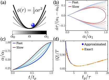
Figure 2: Optimal thermodynamic control of an active particle in a one-dimensional trap. (a) Illustration of an active particle (blue) in a harmonic trap. The protocol consists in driving the trap strength from $\alpha_{0}$ to $\alpha_{1}$. (b) Control speed $\dot{\alpha}$ [Eq.(14)] against trap strength $\alpha$ for different $t_{p}=\{0.1\tau,1\tau,5\tau,10\tau,20\tau,100\tau\}$. (c) Protocols for $t_{p}=\{0.1\tau,\ldots,100\tau\}$. (d) Comparing the scaled heat, where $T=D/\mu$, against protocol duration as approximated in the response framework (blue) [Eq. (8)] and the exact expression (orange) [Eq. (43)]. For both curves, we use the protocols shown in (c). Parameters: $\mu=1$, $D=1$, $D_{1}=0.01$, $\tau=1$, $\alpha_{0}=1$, and $\alpha_{1}=5$.

III.1 Active particle in a harmonic trap

Having established the main framework, we now test it on a toy model consisting of a single active particle in a one-dimensional harmonic trap [Fig. 2(a)]. The motion of the particle is governed by

$$\dot{r}=\mu f+\sqrt{2D}\eta,\quad f=-\alpha r+v/\mu,$$ (42)

where $\phi(\alpha,r)=\alpha r^{2}/2$ is the trap potential, with $\alpha$ being the stiffness. For the self-propulsion, we choose the simplest Ornstein-Uhlenbeck process with $\langle v\rangle=0$ and $\langle v(t)v(s)\rangle=\tau^{-1}D_{1}e^{-|t-s|/\tau}$, where $\tau$ is the persistence time and $D_{1}$ is the amplitude of the active noise. The heat [Eq. (3)] associated with varying $\alpha$ from $\alpha(0)=\alpha_{0}$ to $\alpha(t_{p})=\alpha_{1}$ reads

$$\langle Q\rangle=\frac{\alpha_{0}}{2}\langle r_{0}^{2}\rangle_{\text{s}}-\frac{\alpha_{1}}{2}\langle r_{1}^{2}\rangle+\int_{0}^{t_{p}}dt\bigg{[}\frac{\dot{\alpha}}{2}\langle r^{2}\rangle+\frac{D_{1}}{\tau\mu}-\alpha\langle rv\rangle\bigg{]},$$ (43)

where $r_{0}$ and $r_{1}$ are respectively the initial and final positions of the particle. Since the dynamics in Eq. (42) is linear, the time evolution of the moments $\langle r^{2}\rangle$ and $\langle rv\rangle$ is closed, and can be obtained using Itô’s lemma Gardiner (2009) as

$$\frac{1}{2}\frac{d}{dt}\langle r^{2}\rangle =\langle rv\rangle-\mu\alpha\langle r^{2}\rangle+D,$$ (44)

$$\tau\frac{d}{dt}{\langle rv\rangle} =D_{1}-\langle rv\rangle\left(1+\alpha\mu\tau\right).$$

In steady state, the left-hand side of Eq. (44) is zero, resulting in

$$\langle r^{2}\rangle_{\text{s}}=\frac{1}{\alpha\mu}\left(\frac{D_{1}}{1+\alpha\mu\tau}+D\right),\quad\langle rv\rangle_{\text{s}}=\frac{D_{1}}{1+\alpha\mu\tau}.$$ (45)

Therefore, the heat given in Eq. (43) can be numerically measured for a given protocol $\alpha(t)$ simply by simulating the dynamics of the moments in Eq. (44).

To evaluate the decomposition of heat [Eqs. (8-11)], we use the continuous-state response functions in Eqs. (24) and (26). We show in Appendix D.1 how to obtain the following expressions

$$V =\frac{\alpha D_{1}}{1+\alpha\mu\tau}-\frac{D_{1}}{\mu\tau},\qquad\Sigma=\frac{D_{1}\alpha\mu\tau^{3}}{(1+\alpha\mu\tau)^{4}},$$ (46)

$$\Phi =\frac{D(1+\alpha\mu\tau)^{3}+D_{1}\big{[}1+3\alpha\mu\tau+4(\alpha\mu\tau)^{2}\big{]}}{2(\alpha\mu)^{2}(1+\alpha\mu\tau)^{3}},$$

$$\Lambda =\frac{D(1+\alpha\mu\tau)^{3}+D_{1}\big{[}1+2\alpha\mu\tau-(\alpha\mu\tau)^{2}\big{]}}{2\alpha\mu(1+\alpha\mu\tau)^{3}},$$

$$\Psi =\frac{D}{{4\alpha^{3}\mu^{2}(\alpha\mu\tau+1)^{5}}}\Big{\{}(\alpha\mu\tau+1)^{5}$$

$$\quad+\frac{D_{1}}{D}\big{[}1+5\alpha\mu\tau+11(\alpha\mu\tau)^{2}+3(\alpha\mu\tau)^{3}-16(\alpha\mu\tau)^{4}\big{]}$$

$$\quad-\Big{(}\frac{D_{1}}{D}\Big{)}^{2}(\alpha\mu\tau)^{3}\big{[}8+7\alpha\mu\tau+4(\alpha\mu\tau)^{2}+(\alpha\mu\tau)^{3}\big{]}\Big{\}}.$$

In the passive limit ($D_{1}=0$), the expressions reduce to $\Psi=D/2\alpha^{3}\mu^{2}$, $\Sigma=V=0$, and $\Lambda=\alpha\mu\Phi=D/(2\alpha\mu)$, in agreement with Sivak and Crooks (2012). The protocols for changing the stiffness $\alpha$ of the trap can be readily obtained following the procedure detailed in Sec. II.2. First, we numerically solve the elliptic integral equation in Eq. (15) which connects the constant $E$ with the protocol time $t_{p}$. As $E$ approaches $\underset{\alpha}{\max}\,V$ (namely for increasing $t_{p}$), one needs increasingly high precision to numerically solve Eq. (15). To this end, we utilize the arbitrary-precision numerical library Arb Johansson (2017), that provides a state-of-the-art numerical integration procedure based upon adaptive bisection and adaptive Gaussian quadrature Johansson (2018). Second, we obtain the protocol trajectory $\alpha(t)$ by numerically solving Eq. (14), for given protocol time $t_{p}$ and boundary conditions $\{\alpha_{0},\alpha_{1}\}$. We report the results of optimal protocols for different $t_{p}$ in Figs. 2(b-c). Very fast ($t_{p}\ll t_{p}^{*}$) and very slow ($t_{p}\gg t_{p}^{*}$) protocols collapse onto two separate master curves. This is in contrast with the thermodynamic control of passive systems, where there is only a single protocol master curve valid for all protocol durations Deffner and Bonança (2020).

For the optimal protocols in Fig. 2(c), we then compare two separate evaluations of heat. We either (i) simulate the dynamics in Eq. (44) with the optimal protocol, and measure the corresponding heat [Eq. (43)], or (ii) directly substitute the optimal protocol in the expression of heat given in Eq. (8), which relies on response theory. Comparing these two results allows us to delineate the regime where the response theory is indeed valid. We report in Fig. 2(d) that the two evaluations of heat match very well not only at large $t_{p}$, where the heat scales linearly with $t_{p}$, but also in the regime where the heat is minimum ($t_{p}\simeq t_{p}^{\ast}$). At times smaller than $t_{p}^{*}$, a discrepancy arises, showing that the assumption of slow driving, underpinning the response framework, breaks down in this regime.

For a general potential, we expect that the protocol time at minimum heat $t_{p}^{*}$ increases as the activity gets weaker ($|{\bf v}_{i}|\to 0$). For the harmonic case treated here, we evaluate analytically the approximated estimation of $t_{p}^{*}$, which stems from matching the asymptotic behaviors of the heat, by substituting Eq. (46) into Eqs. (17) and (58). This estimation of $t_{p}^{*}$ captures the divergence $t_{p}^{*}\sim 1/\sqrt{D_{1}}$ at small activity ($D_{1}/D\ll 1$). Interestingly, it also predicts that $t_{p}^{*}$ should plateau to a finite value at large activity ($D_{1}/D\gg 1$), as shown in Fig. 3.

Figure 3: Optimal protocol duration $t_{p}^{\ast}$ as a function of the active noise amplitude $D_{1}$, as predicted by the scaling relation Eq. (17) in conjunction with Eq. (46). Parameters: $\alpha_{0}/\alpha_{1}=1/5,\mu=\tau=D=1$.

III.2 Repulsive active Brownian particles (RABPs)

Having successfully tested our framework on a rather simple model, we now apply it to a many-body active system which features richer physics. Specifically, we consider a system of $N$ RABPs in two spatial dimensions that can exhibit MIPS [Fig 4]Cates and Tailleur (2015). We take the dynamics in Eq. (1) with the potential energy given by

$$\phi=\frac{1}{2}\sum_{i,j\neq i}U_{ij},$$ (47)

where the pair potential $U_{ij}$ depends on the inter-particle distance $r_{ij}=|{\bf r}_{i}-{\bf r}_{j}|$. To impose repulsive interactions, we take $U_{ij}=\varepsilon\exp\big{[}-1/(1-(r_{ij}/\alpha)^{2})\big{]}$ for $r_{ij}<\alpha$, and $U_{ij}=0$ otherwise. The control parameter $\alpha$ here embodies the range of the repulsive interaction, which is akin to the excluded-volume radius. Therefore, changing $\alpha$ at a fixed number of particles amounts to changing the packing fraction, which can lead to a transition between homogeneous and phase-separated states [Fig 4]. Moreover, we define the self-propulsion of particle $i$ as

$$\mathbf{v}_{i}=v_{0}\,(\cos\theta_{i},\sin\theta_{i}),\quad\dot{\theta}_{i}=\sqrt{2/\tau}\zeta_{i},$$ (48)

where $v_{0}$ is the constant magnitude of self-propulsion speed, and $\zeta_{i}$ is a Gaussian white noise with zero mean and unit variance. The persistence time $\tau$, which controls the angular noise, determines the self-propulsion correlations as $\langle v_{in}(t)v_{im}(0)\rangle=\delta_{ij}\delta_{nm}v_{0}^{2}e^{-|t|/\tau}$, where $n$ and $m$ refer to spatial coordinates Fodor and Marchetti (2018).

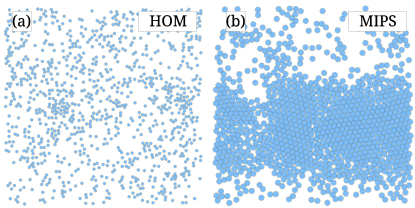
Figure 4: Simulation snapshots of the repulsive active Brownian particles showing two distinct phases determined by the particle size $\alpha$. (a) Small size of particles ($\alpha v/D=2\times 10^{3}$) results in a homogeneous phase (HOM), whilst (b) larger size of particles ($\alpha v/D=4\times 10^{3}$) leads to motility-induced phase separation (MIPS).

Due to the difficulty in deriving analytical expressions for the decomposition of heat [Eqs. (8-11)], we resort to numerically evaluating the corresponding averages and correlations given in Appendix D.2. We perform simulations at different particle sizes $\{\alpha\}$ in the homogeneous case ($2.1\times 10^{3}<\alpha v/D<2.4\times 10^{3}$), and in the case of phase separation ($3.0\times 10^{3}<\alpha v/D<3.3\times 10^{3}$). After obtaining data for various $\alpha$ values, we fit averages and correlations to deduce their continuous dependence in terms of $\alpha$. We then use these fitting functions to obtain the control protocols through solving Eq. (15), where again we distinguish protocols for the homogeneous and MIPS cases. In practice, we consider $N=2000$ for RABPs in a square box of side length $L=200$, with periodic boundary conditions to mimic bulk conditions. The parameters are $v=1$, $\mu=1$, $D=10^{-3}$, $\tau=10^{2}$, and $\varepsilon=10^{2}T$. Considering that lengthscales and timescales are respectively taken in units of micrometers and seconds, the parameter values are chosen to be relevant to actual microswimmers Fodor and Marchetti (2018), such as moving bacteria. We integrate the equation of motions [Eqs. (1) and (48)] using a standard Euler discrete-update rule.

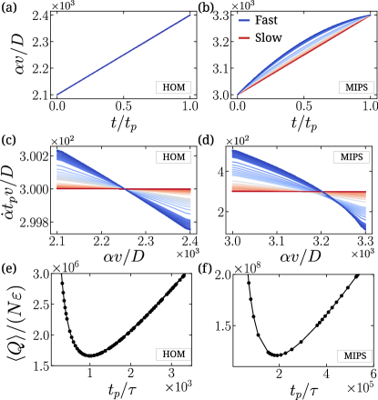
Figure 5: Optimal thermodynamic control of a many-body system consisting of repulsive active Brownian particles in the homogeneous (HOM) (left) and phase-separated (MIPS) (right) cases. (a-b) Derived protocols for driving the particle size $\alpha$ as a function of time. (c-d) Control speed $\dot{\alpha}$ against control parameter $\alpha$. (e-f) Scaled heat against protocol duration, computed using protocols shown in (a-b).

The resulting control protocols are shown in Figs. 5(a-b). In the homogeneous case, the control protocols appear to lie on a single master curve, as for the control of passive systems Deffner and Bonança (2020). In contrast, for the MIPS case, we obtain various protocol curves for different protocol durations $t_{p}$, which collapse into distinct master curves either for very fast and very slow protocols. Interestingly, plotting the control speed $\dot{\alpha}$ against the value of the control parameter $\alpha$ reveals that the protocol curves do not actually collapse onto a single master curve in the homogeneous case [Fig. 5(c)], although the change in control speed is clearly smaller than that of the MIPS case [Fig. 5(d)]. Since the existence of a single master curve is a signature of passive systems Deffner and Bonança (2020), we speculate that RAPBs in the homogeneous state have macroscopic signatures that resemble a thermal system, at least as far as the heat decomposition [Eqs. (8-11)] is concerned. Finally, we compute the heat as predicted from the response framework [Eq. (8)]. The optimal protocol duration $t_{p}^{\ast}/\tau\approx 1\times 10^{3}$ in the homogeneous case [Fig. 5(e)] is approximately 200 times larger than in the MIPS case, where $t_{p}^{\ast}/\tau\approx 2\times 10^{5}$ [Fig. 5(f)]. This difference illustrates that the response to changes in particle size is slower in the MIPS case, where the cluster size adapts to the packing fraction, than in the homogeneous case.

IV Discussion

We have derived a thermodynamic framework for the optimal control of active systems that operate arbitrarily far from thermal equilibrium. The systematic nature of our approach relies on recent advances in stochastic thermodynamics and response theory, as inspired by previous works on the thermodynamic control of passive systems Crooks (2007); Sivak and Crooks (2012). Applications of our framework have revealed new insights into the control of active systems that are in direct contrast to the passive case. Specifically, we have found that: (i) for non-zero activity, expanding the dissipation to linear order in the protocol duration requires knowledge of the second-order response, whereas linear response is sufficient to obtain the same order in the passive case Sivak and Crooks (2012); (ii) there is a cost (dissipation) associated with the self-driving meaning that the optimal duration is not the longest one, at variance with passive systems Sivak and Crooks (2012); Large and Sivak (2019); (iii) we find that each protocol duration gives rise to a unique protocol curve which eventually collapse onto either a fast or slow master curve, in contrast to the strict many-to-one mapping as seen in passive control Deffner and Bonança (2020); Zhong and DeWeese (2022).

As a demonstration of the generality of our approach, we have built our framework to describe both continuous and discrete-state active systems. This opens the door to future work that may quantitatively compare optimal control scenarios between these different categories of active matter. Interestingly, different definitions of irreversibility and of dissipation have been proposed for various models of active matter Fodor et al. (2016); Speck (2016); Gaspard and Kapral (2019, 2020); Fodor and Cates (2021). Indeed, the measure of irreversibility provides a legitimate quantification of dissipation only if the underlying dynamics satisfies specific thermodynamic constraints. Our results on discrete-state dynamics can be regarded as a motivation to develop active discrete-state models that satisfy these constraints thermodynamically. Moreover, our approach could also be adapted to field theories of active matter Nardini et al. (2017); Chaté (2020); Øyvind L Borthne et al. (2020), some of which can be embedded within linear irreversible thermodynamics Markovich et al. (2021). Furthermore, although we have focused on optimizing heat, our framework can be straightforwardly adapted to other cost functions, for instance the extracted work (which has been optimized in the literature of passive systems Schmiedl and Seifert (2007); Gomez-Marin et al. (2008); Sivak and Crooks (2012); Zulkowski et al. (2012, 2013); Bonança and Deffner (2014); Rotskoff and Crooks (2015); Rotskoff et al. (2017); Deffner and Bonança (2020); Zhong and DeWeese (2022); Blaber and Sivak (2023)). Note that a recent study has considered optimizing the work in active matter by directly applying the framework of passive systems Gupta et al. (2023).

Our framework relies on the assumption of weak and slow driving of the control parameter. It leads to an explicit decomposition of heat which can serve as a seed, or a testing ground, for machine learning approaches beyond the smooth-driving assumptions Falk et al. (2021); Engel et al. (2022). Interestingly, one could extend our framework to take into account corrections from higher-order responses, and thus to capture faster driving, within a systematic approach. Moreover, although we have focused here on controlling a single parameter for simplicity, it would be interesting to consider an arbitrary number of control variables in future works. Lastly, encouraged by the experimental implementations of the control framework in passive systems Tafoya et al. (2019); Scandi et al. (2022) and recent progress in measuring the response of living systems Toyabe et al. (2010); Turlier et al. (2016); Ahmed et al. (2018); Ariga et al. (2018), our framework can be readily deployed by experimentalists to explore the control of experimental active systems. Indeed, even without knowing the nonequilibrium response-correlation relation in Sec. II.3, our decomposition of heat in Eqs. (8-11) already delineates which perturbation to apply and which response to measure. We anticipate that the potential success of applications of our framework will heavily depend on the quality of measured response functions.

Overall, our work paves the way towards designing active materials able to optimally switch between collective states. Indeed, while most studies of active matter focus on establishing phase diagrams, by associating control parameter values with collective states Marchetti et al. (2013); Gompper et al. (2020), how to optimally induce transitions has remained largely unexplored. While our framework sets the stage to this end, there remains a series of open challenges. First, the assumption of slow driving precludes crossing a critical transition, since the relaxation of the system is always slower than any perturbation at criticality del Campo and Zurek (2014). Considering non-critical transitions instead, the corresponding order parameter is typically discontinuous, and so are the averages and correlations in the heat decomposition. Accordingly, one expects that the optimal protocol is no longer smooth when crossing phase boundaries, which challenges the assumption of weak driving. Therefore, it remains to be explored how the assumptions underlying the response framework need to be adapted when switching between collective states in active matter.

Appendix A Decomposition of heat

In this Appendix, we derive the decomposition of heat given in Eqs. (8-11). To this end, we assume that the control parameter $\alpha$ is varying both weakly and slowly, which allows us to rely on (i) the representation of averages in terms of response functions [Eq. (6)], and (ii) the expansion of the control parameter variation in terms of time increments [Eq. (7)]. Using these approximations, we first simplify the averages featuring in the heat definition [Eq. (3)]. We first expand $\langle\phi_{1}\rangle$ as

$$\langle\phi_{1}\rangle \approx\langle\phi_{1}\rangle_{\text{s}}+\int_{-\infty}^{t_{p}}dt^{\prime}\Delta\alpha_{t_{p},t^{\prime}}R_{1}(\phi;t_{p},t^{\prime}),$$ (49)

$$\approx\langle\phi_{1}\rangle_{\text{s}}+\dot{\alpha}_{1}\int_{0}^{\infty}dtR_{1}(\phi;t,0)t,$$

where we have used the approximations (i) and (ii) in the first and second lines, respectively. Similarly, we deduce $\langle\partial_{\alpha}\phi\rangle$ as

$$\langle\partial_{\alpha}\phi(t)\rangle \approx\langle\partial_{\alpha}\phi\rangle_{\text{s}}+\int_{-\infty}^{t}dt^{\prime}\Delta\alpha_{t,t^{\prime}}R_{1}(\partial_{\alpha}\phi;t,t^{\prime})$$ (50)

$$\approx\langle\partial_{\alpha}\phi\rangle_{\text{s}}+\dot{\alpha}(t)\int_{0}^{\infty}dt^{\prime}R_{1}(\partial_{\alpha}\phi;t^{\prime},0)t^{\prime}.$$

Finally, $\langle J\rangle$ follows as

$$\langle J(t)\rangle \approx\langle J\rangle_{\text{s}}+\int_{-\infty}^{t}dt^{\prime}\Delta\alpha_{t,t^{\prime}}R_{1}(J;t,t^{\prime})$$ (51)

$$\quad+\int_{-\infty}^{t}\int_{-\infty}^{t}dtdt^{\prime}\Delta\alpha_{t,t^{\prime}}\Delta\alpha_{t,t^{\prime\prime}}R_{2}(J;t,t^{\prime},t^{\prime\prime}),$$

$$\approx\langle J\rangle_{\text{s}}+\dot{\alpha}(t)\int_{0}^{\infty}dt^{\prime}R_{1}(J;t^{\prime},0)t^{\prime}$$

$$\quad+\frac{\ddot{\alpha}(t)}{2}\int_{0}^{\infty}dt^{\prime}R_{1}(J;t^{\prime},0){t^{\prime}}^{2}$$

$$\quad+\dot{\alpha}(t)^{2}\int_{0}^{\infty}\int_{0}^{\infty}dt^{\prime}dt^{\prime\prime}R_{2}(J;t^{\prime},t^{\prime}-t^{\prime\prime},0)t^{\prime}t^{\prime\prime}.$$

In contrast with Eqs. (49-50), for Eq. (51) we have used the second-order response $R_{2}$, and also the expansion of $\Delta\alpha$ up to second order in $\Delta t$ [Eq. (7)]. These higher-order corrections are needed for consistency in the overall expansion of the heat, to leading order in $\dot{\alpha}$. Substituting Eqs. (49-51) into Eq. (3), then integrating the second last term in Eq. (51) by parts, we deduce the expression of the boundary and Lagrangian terms in the heat [Eqs. (8-11)].

Appendix B Scalings of heat

In this Appendix, we examine how the heat $\langle Q\rangle$ scales with the protocol time $t_{p}$ by considering the asymptotic regimes for fast protocols ($t_{p}\ll t_{p}^{\ast}$) and slow protocols ($t_{p}\gg t_{p}^{\ast}$), where $t_{p}^{*}$ minimizes $\langle Q\rangle$ [Fig. 1]. We rely on the decomposition $\langle Q\rangle=B+\int dt{\cal L}$ given in terms of the boundary and Lagrangian contributions [Eqs. (8-11)], respectively denoted by $B$ and $\cal L$. Besides, we express $\cal L$ as

$${\cal L}=E-2V,$$ (52)

where we have introduced the constant of motion $E$, defined in Eq. (13).

First, it appears from Eqs. (14-15) that the protocol duration $t_{p}$ is small whenever the constant of motion $E$ satisfies $E\gg\underset{\alpha}{\max}\,V$. For fast protocols ($t_{p}\ll t_{p}^{*}$), we can then simplify Eqs. (14-15) as

$$E \underset{t_{p}\ll t_{p}^{*}}{\sim}\frac{1}{t_{p}^{2}}\bigg{[}\int_{\alpha_{0}}^{\alpha_{1}}d\alpha\sqrt{(\Psi-\Sigma^{\prime})(\alpha)}\bigg{]}^{2},$$ (53)

$$\dot{\alpha} \underset{t_{p}\ll t_{p}^{*}}{\sim}\pm\sqrt{\frac{E}{(\Psi-\Sigma^{\prime})(\alpha)}}.$$

Substituting the expression of $E$ into that of $\dot{\alpha}$, we deduce after separating variables and integration that the optimal protocol obeys

$$\int_{\alpha_{0}}^{\alpha(t)}d\alpha\sqrt{(\Psi-\Sigma^{\prime})(\alpha)}\underset{t_{p}\ll t_{p}^{*}}{\approx}\frac{t}{t_{p}}\int_{\alpha_{0}}^{\alpha_{1}}d\alpha\sqrt{(\Psi-\Sigma^{\prime})(\alpha)},$$ (54)

where we have assumed $\alpha_{0}<\alpha_{1}$. Therefore, it follows that the optimal trajectory $\alpha(t)$ follows a master curve when scaling $t$ with $t_{p}$, as for the control of passive systems Sivak and Crooks (2012). Moreover, the condition $E\gg\underset{\alpha}{\max}\,V$ yields

$$\int_{0}^{t_{p}}dt{\cal L}\underset{t_{p}\ll t_{p}^{\ast}}{\sim}E\,t_{p},$$ (55)

and we express the boundary term [Eq. (9)], using the simplified expression of $\dot{\alpha}$ [Eq. (53)], as

$$B\underset{t_{p}\ll t_{p}^{\ast}}{\sim}\sqrt{E}\,\bigg{[}\frac{\Sigma}{\sqrt{\Psi-\Sigma^{\prime}}}(\alpha_{0})-\frac{\Sigma+\Phi}{\sqrt{\Psi-\Sigma^{\prime}}}(\alpha_{1})\bigg{]},$$ (56)

where we have ignored terms that do not depend on $t_{p}$. Finally, combining Eqs. (55-56) with the fact that $E\sim 1/t_{p}^{2}$ [Eq. (53)] results in the first scaling relation for the heat:

$$\langle Q\rangle\underset{t_{p}\ll t_{p}^{\ast}}{\sim}K(\alpha_{0},\alpha_{1})/t_{p},$$ (57)

where

$$K(\alpha_{0},\alpha_{1}) =c(\alpha_{0},\alpha_{1})\bigg{[}\frac{\Sigma}{\sqrt{\Psi-\Sigma^{\prime}}}(\alpha_{0})-\frac{\Sigma+\Phi}{\sqrt{\Psi-\Sigma^{\prime}}}(\alpha_{1})\bigg{]}$$ (58)

$$\quad+c(\alpha_{0},\alpha_{1})^{2},$$

$$c(\alpha_{0},\alpha_{1}) =\int_{\alpha_{0}}^{\alpha_{1}}d\alpha\sqrt{(\Psi-\Sigma^{\prime})(\alpha)}.$$

The term $K$ accounts for contributions from both the boundary and Lagrangian terms.

Second, we deduce from Eqs. (14-15) that the protocol duration $t_{p}$ is large whenever $E\approx\underset{\alpha}{\max}\,V$. Therefore, for slow protocols ($t_{p}\gg t_{p}^{*}$), the constant of motion $E$ depends only weakly on the protocol duration $t_{p}$. It follows from Eq. (14) that the protocol speed $\dot{\alpha}(t)$ depends weakly on $t_{p}$, and so does the boundary term $B$ [Eq. (9)]. Plugging the condition $E\approx\underset{\alpha}{\max}\,V$ into Eq. (52), and integrating over the protocol results in

$$\int_{0}^{t_{p}}dt{\cal L}\underset{t_{p}\gg t_{p}^{\ast}}{\sim}-t_{p}\max_{\alpha}V.$$ (59)

Therefore, we arrive at the second scaling relation for the heat:

$$\langle Q\rangle\underset{t_{p}\gg t_{p}^{\ast}}{\sim}t_{p}\min_{\alpha}\langle J\rangle_{\text{s}},$$ (60)

where we have used $V=-\langle J\rangle_{\text{s}}$.

Appendix C Response theory from path probability

In this Appendix, we show how to explicitly relate response and correlation functions using a path probability representation of the dynamics. We consider two cases: (i) continuous-state dynamics [Eq. (1)], and (ii) discrete-state dynamics [Eq. (28)].

C.1 Continuous-state dynamics

The linear response function $R_{1}$, defined in Eq. (18), can be written in terms of the dynamic action $\cal S$ [Eq. (23)] as

$$R_{1}({X};t,t^{\prime})$$ (61)

$$=\int{X}(t)\bigg{[}\frac{\delta\mathcal{N}}{\delta\Delta\alpha_{t,t^{\prime}}}-{\cal N}\frac{\delta\mathcal{S}}{\delta\Delta\alpha_{t,t^{\prime}}}\bigg{]}_{\Delta\alpha\to 0}e^{-{\cal S}}\,\mathcal{D}[{\bm{\eta}},{\bf v}],$$

where ${\cal N}=1/\int e^{-{\cal S}}\mathcal{D}[{\bm{\eta}},{\bf v}]$. Given that

$$\frac{\delta\mathcal{N}}{\delta\Delta\alpha}\bigg{|}_{\Delta\alpha\to 0} ={\cal N}^{2}\int\frac{\delta\mathcal{S}}{\delta\Delta\alpha}\bigg{|}_{\Delta\alpha\to 0}e^{-{\cal S}}\,\mathcal{D}[{\bm{\eta}},{\bf v}]$$ (62)

$$={\cal N}\left\langle\frac{\delta\mathcal{S}}{\delta\Delta\alpha}\right\rangle_{\text{s}}\bigg{|}_{\Delta\alpha\to 0},$$

we deduce

$$R_{1}({X};t,t^{\prime}) =\bigg{[}\langle X\rangle_{\text{s}}\left\langle\frac{\delta\mathcal{S}}{\delta\Delta\alpha}\right\rangle_{\text{s}}-\left\langle X(t)\frac{\delta\mathcal{S}}{\delta\Delta\alpha_{t,t^{\prime}}}\right\rangle\bigg{]}_{\Delta\alpha\to 0}$$ (63)

$$=-\mathopen{\hbox{\set@color${\bigg{\langle}}$}\kern-1.94444pt\leavevmode\hbox{\set@color${\bigg{\langle}}$}}X(t)\frac{\delta\mathcal{S}}{\delta\Delta\alpha_{t,t^{\prime}}}\mathclose{\hbox{\set@color${\bigg{\rangle}}$}\kern-1.94444pt\leavevmode\hbox{\set@color${\bigg{\rangle}}$}}_{\Delta\alpha\to 0},$$

where we have used Eq. (25). From Eq. (23), we get

$$\frac{\delta\mathcal{S}}{\delta\Delta\alpha}\bigg{|}_{\Delta\alpha\to 0} =-\frac{1}{2T}\bigg{[}(\nabla_{i}\partial_{\alpha}\phi)\cdot(\dot{\bf r}_{i}-\mu{\bf f}_{i})\bigg{]}$$ (64)

$$=-\frac{1}{2T}\bigg{[}\partial_{\alpha}\dot{\phi}-\mu(\nabla_{i}\partial_{\alpha}\phi)\cdot{\bf f}_{i})\bigg{]},$$

where we have used the chain rule $\partial_{\alpha}\dot{\phi}=\dot{\bf r}_{i}\cdot\nabla_{i}\partial_{\alpha}\phi$ in the unperturbed dynamics (namely, at constant $\alpha$). Finally, substituting Eq. (64) into Eq. (63) yields the expression for the linear response function

$$2TR_{1}(X;t,t^{\prime})=\frac{d}{dt^{\prime}}\mathopen{\hbox{\set@color${\big{\langle}}$}\kern-1.94444pt\leavevmode\hbox{\set@color${\big{\langle}}$}}{X}_{t}[\partial_{\alpha}\phi]_{t^{\prime}}\mathclose{\hbox{\set@color${\big{\rangle}}$}\kern-1.94444pt\leavevmode\hbox{\set@color${\big{\rangle}}$}}-\mu\mathopen{\hbox{\set@color${\big{\langle}}$}\kern-1.94444pt\leavevmode\hbox{\set@color${\big{\langle}}$}}X_{t}\big{[}(\nabla_{i}\partial_{\alpha}\phi)\cdot\mathbf{f}_{i}\big{]}_{t^{\prime}}\mathclose{\hbox{\set@color${\big{\rangle}}$}\kern-1.94444pt\leavevmode\hbox{\set@color${\big{\rangle}}$}},$$ (65)

in agreement with in Eq. (24). Symmetrizing the linear response function results in the following

$$R_{1}(X;t,t^{\prime})-R_{1}(X;t^{\prime},t)$$ (66)

$$\quad=\frac{1}{2T}\bigg{[}\frac{d}{dt^{\prime}}\mathopen{\hbox{\set@color${\langle}$}\kern-1.94444pt\leavevmode\hbox{\set@color${\langle}$}}X_{t}[\partial_{\alpha}\phi]_{t^{\prime}}\mathclose{\hbox{\set@color${\rangle}$}\kern-1.94444pt\leavevmode\hbox{\set@color${\rangle}$}}-\mu\mathopen{\hbox{\set@color${\langle}$}\kern-1.94444pt\leavevmode\hbox{\set@color${\langle}$}}X_{t}[(\nabla_{i}\partial_{\alpha}\phi)\cdot\mathbf{f}_{i}]_{t^{\prime}}\mathclose{\hbox{\set@color${\rangle}$}\kern-1.94444pt\leavevmode\hbox{\set@color${\rangle}$}}$$

$$\qquad-\frac{d}{dt}\mathopen{\hbox{\set@color${\langle}$}\kern-1.94444pt\leavevmode\hbox{\set@color${\langle}$}}X_{t^{\prime}}[\partial_{\alpha}\phi]_{t}\mathclose{\hbox{\set@color${\rangle}$}\kern-1.94444pt\leavevmode\hbox{\set@color${\rangle}$}}+\mu\mathopen{\hbox{\set@color${\langle}$}\kern-1.94444pt\leavevmode\hbox{\set@color${\langle}$}}X_{t^{\prime}}[(\nabla_{i}\partial_{\alpha}\phi)\cdot\mathbf{f}_{i}]_{t}\mathclose{\hbox{\set@color${\rangle}$}\kern-1.94444pt\leavevmode\hbox{\set@color${\rangle}$}}\bigg{]}.$$

In the passive case ($\mathbf{v}=0$), the force acting on particles reduces to ${\bf f}_{i}=-\nabla_{i}\phi$. Besides, time-reversal symmetry yields $\mathopen{\hbox{\set@color${\langle}$}\kern-1.94444pt\leavevmode\hbox{\set@color${\langle}$}}X_{t}Y_{t^{\prime}}\mathclose{\hbox{\set@color${\rangle}$}\kern-1.94444pt\leavevmode\hbox{\set@color${\rangle}$}}=\mathopen{\hbox{\set@color${\langle}$}\kern-1.94444pt\leavevmode\hbox{\set@color${\langle}$}}X_{t^{\prime}}Y_{t}\mathclose{\hbox{\set@color${\rangle}$}\kern-1.94444pt\leavevmode\hbox{\set@color${\rangle}$}}$ and $(d/dt)\mathopen{\hbox{\set@color${\langle}$}\kern-1.94444pt\leavevmode\hbox{\set@color${\langle}$}}X_{t^{\prime}}Y_{t}\mathclose{\hbox{\set@color${\rangle}$}\kern-1.94444pt\leavevmode\hbox{\set@color${\rangle}$}}=-(d/dt^{\prime})\mathopen{\hbox{\set@color${\langle}$}\kern-1.94444pt\leavevmode\hbox{\set@color${\langle}$}}X_{t}Y_{t^{\prime}}\mathclose{\hbox{\set@color${\rangle}$}\kern-1.94444pt\leavevmode\hbox{\set@color${\rangle}$}}$ for time-symmetric observables $X$ and $Y$ Onsager (1931). Causality enforce that $R_{1}(X;t^{\prime},t)=0$ for $t^{\prime}<t$, from which we deduce

$$R(X;t,t^{\prime})=\frac{1}{T}\frac{d}{dt^{\prime}}\mathopen{\hbox{\set@color${\langle}$}\kern-1.94444pt\leavevmode\hbox{\set@color${\langle}$}}X_{t}[\partial_{\alpha}\phi]_{t^{\prime}}\mathclose{\hbox{\set@color${\rangle}$}\kern-1.94444pt\leavevmode\hbox{\set@color${\rangle}$}},$$ (67)

as predicted by the fluctuation-dissipation theorem Kubo (1966).

Similarly, we can write the second-order response function $R_{2}$, defined in Eq. (18), as

$$R_{2} ({X};t,t^{\prime},t^{\prime\prime})$$ (68)

$$=\int{X}(t)\bigg{[}{\cal N}\bigg{(}\frac{\delta\mathcal{S}}{\delta\Delta\alpha_{t,t^{\prime}}}\frac{\delta\mathcal{S}}{\delta\Delta\alpha_{t,t^{\prime\prime}}}-\frac{\delta^{2}\mathcal{S}}{\delta\Delta\alpha_{t,t^{\prime}}\delta\Delta\alpha_{t,t^{\prime\prime}}}\bigg{)}$$

$$\quad-\frac{\delta\mathcal{N}}{\delta\Delta\alpha_{t,t^{\prime\prime}}}\frac{\delta\mathcal{S}}{\delta\Delta\alpha_{t,t^{\prime}}}-\frac{\delta\mathcal{N}}{\delta\Delta\alpha_{t,t^{\prime}}}\frac{\delta\mathcal{S}}{\delta\Delta\alpha_{t,t^{\prime\prime}}}$$

$$\quad+\frac{\delta^{2}\mathcal{N}}{\delta\Delta\alpha_{t,t^{\prime}}\delta\Delta\alpha_{t,t^{\prime\prime}}}\bigg{]}_{\Delta\alpha\to 0}e^{-{\cal S}}\,\mathcal{D}[{\bm{\eta}},{\bf v}].$$

Given that

$$\frac{\delta^{2}\mathcal{N}}{\delta\Delta\alpha_{t,t^{\prime}}\delta\Delta\alpha_{t,t^{\prime\prime}}}\bigg{|}_{\Delta\alpha\to 0}$$ (69)

$$\quad={\cal N}\,\bigg{[}\left\langle\frac{\delta^{2}\mathcal{S}}{\delta\Delta\alpha_{t,t^{\prime}}\delta\Delta\alpha_{t,t^{\prime\prime}}}-\frac{\delta\mathcal{S}}{\delta\Delta\alpha_{t,t^{\prime}}}\frac{\delta\mathcal{S}}{\delta\Delta\alpha_{t,t^{\prime\prime}}}\right\rangle$$

$$\qquad+2\left\langle\frac{\delta\mathcal{S}}{\delta\Delta\alpha_{t,t^{\prime}}}\right\rangle_{\text{s}}\left\langle\frac{\delta\mathcal{S}}{\delta\Delta\alpha_{t,t^{\prime\prime}}}\right\rangle_{\text{s}}\bigg{]}_{\Delta\alpha\to 0},$$

we deduce

$$R_{2}({X};t,t^{\prime},t^{\prime\prime}) =\mathopen{\hbox{\set@color${\bigg{\langle}}$}\kern-1.94444pt\leavevmode\hbox{\set@color${\bigg{\langle}}$}\kern-1.94444pt\leavevmode\hbox{\set@color${\bigg{\langle}}$}}X(t)\bigg{[}\frac{\delta\mathcal{S}}{\delta\Delta\alpha_{t,t^{\prime}}}\frac{\delta\mathcal{S}}{\delta\Delta\alpha_{t,t^{\prime\prime}}}$$ (70)

$$\quad\qquad-\frac{\delta^{2}\mathcal{S}}{\delta\Delta\alpha_{t,t^{\prime}}\delta\Delta\alpha_{t,t^{\prime\prime}}}\bigg{]}\mathclose{\hbox{\set@color${\bigg{\rangle}}$}\kern-1.94444pt\leavevmode\hbox{\set@color${\bigg{\rangle}}$}\kern-1.94444pt\leavevmode\hbox{\set@color${\bigg{\rangle}}$}}_{\Delta\alpha\to 0},$$

where we have used Eq. (27). From Eq. (23), we get

$$\frac{\delta^{2}\mathcal{S}}{\delta\Delta\alpha_{t,t^{\prime}}\delta\Delta\alpha_{t,t^{\prime\prime}}}\bigg{|}_{\Delta\alpha\to 0}$$ (71)

$$\;=\frac{\delta(t^{\prime}-t^{\prime\prime})}{2T}\Big{[}\mu(\nabla_{i}\partial_{\alpha}\phi)^{2}+(\nabla_{i}\partial_{\alpha}^{2}\phi)\cdot(\dot{\mathbf{r}}_{i}-\mu\mathbf{f}_{i})\Big{]}.$$

Finally, substituting Eqs. (64) and (71) into Eq. (70) yields the expression for the second-order response function given in Eq. (26).

C.2 Discrete-state dynamics

We can repeat the above derivation for the case of discrete-state dynamics. The response functions can be written in terms of perturbations of the dynamic action ${\cal A}$ [Eq. (38)] as

$$R_{1}({X};t,t^{\prime}) =-\mathopen{\hbox{\set@color${\bigg{\langle}}$}\kern-1.94444pt\leavevmode\hbox{\set@color${\bigg{\langle}}$}}X(t)\frac{\delta\mathcal{A}}{\delta\Delta\alpha_{t,t^{\prime}}}\mathclose{\hbox{\set@color${\bigg{\rangle}}$}\kern-1.94444pt\leavevmode\hbox{\set@color${\bigg{\rangle}}$}}_{\Delta\alpha\to 0},$$ (72)

$$R_{2}({X};t,t^{\prime},t^{\prime\prime}) =\mathopen{\hbox{\set@color${\bigg{\langle}}$}\kern-1.94444pt\leavevmode\hbox{\set@color${\bigg{\langle}}$}\kern-1.94444pt\leavevmode\hbox{\set@color${\bigg{\langle}}$}}X(t)\bigg{[}\frac{\delta\mathcal{A}}{\delta\Delta\alpha_{t,t^{\prime}}}\frac{\delta\mathcal{A}}{\delta\Delta\alpha_{t,t^{\prime\prime}}}$$

$$\quad\qquad-\frac{\delta^{2}\mathcal{A}}{\delta\Delta\alpha_{t,t^{\prime}}\delta\Delta\alpha_{t,t^{\prime\prime}}}\bigg{]}\mathclose{\hbox{\set@color${\bigg{\rangle}}$}\kern-1.94444pt\leavevmode\hbox{\set@color${\bigg{\rangle}}$}\kern-1.94444pt\leavevmode\hbox{\set@color${\bigg{\rangle}}$}}_{\Delta\alpha\to 0}.$$

From Eq. (38), we get

$$\frac{\delta\mathcal{A}}{\delta\Delta\alpha}\bigg{|}_{\Delta\alpha\rightarrow 0} =\frac{1}{2T}\sum_{i,j\neq i}\Big{[}K_{ij}\rho_{j}\partial_{\alpha}\phi_{i}-n_{ij}\partial_{\alpha}(\phi_{i}-\phi_{j})\Big{]}$$ (73)

$$=\frac{1}{2T}\bigg{(}\sum_{i,j\neq i}K_{ij}\rho_{j}\partial_{\alpha}\phi_{i}-\partial_{\alpha}\dot{\phi}\bigg{)},$$

where we have used that $\sum_{i}K_{ij}=0$, which follows from $\sum_{i}\dot{p}_{i}=0$ and Eq. (28), and also $\partial_{\alpha}\dot{\phi}=\sum_{i,j\neq i}n_{ij}\partial_{\alpha}(\phi_{i}-\phi_{j})$ in the unperturbed dynamics. Similarly, one can use Eq. (38) to show that

$$\frac{\delta^{2}\mathcal{A}}{\delta\Delta\alpha_{t,t^{\prime}}\delta\Delta\alpha_{t,t^{\prime\prime}}}\bigg{|}_{\Delta\alpha\to 0}$$ (74)

$$=\frac{\delta(t^{\prime}-t^{\prime\prime})}{2T}\sum_{i,j}\Big{[}K_{ij}\rho_{j}\Big{(}\partial^{2}_{\alpha}\phi_{i}-\frac{(\partial_{\alpha}\phi_{j}-\partial_{\alpha}\phi_{i})^{2}}{2T}\Big{)}$$

$$\qquad+n_{ij}\partial^{2}_{\alpha}(\phi_{i}-\phi_{j})\Big{]}.$$

Combining Eqs. (72-74) gives the discrete-state response functions in Eqs. (39-40).

Appendix D Applications of thermodynamic control

In this Appendix, we determine how the generic decomposition of heat, given in Eqs. (8-11) for arbitrary potential $\phi$ and self-propulsion ${\bf v}_{i}$, translates in two specific cases. We consider the two examples discussed in the main text: an active particle in harmonic trap [Sec. III.1], and an assembly of active particles with purely repulsive interactions [Sec. III.2].

D.1 Control of trap stiffness

In the case of an active particle in a one-dimensional harmonic trap, we have $\phi=\frac{1}{2}\alpha r^{2}$ for the potential energy, yielding: $\partial_{\alpha}\phi=\frac{1}{2}r^{2}$, $\nabla\phi=\alpha r$, and $\nabla\partial_{\alpha}\phi=r$. The functions in the decomposition of heat [Eqs. (8-11)] then read

$$\Sigma =\frac{\alpha}{4T}\int_{0}^{\infty}dt\Bigg{[}\mathopen{\hbox{\set@color${\langle}$}\kern-1.94444pt\leavevmode\hbox{\set@color${\langle}$}}{}[rv]_{t}[rv]_{0}\mathclose{\hbox{\set@color${\rangle}$}\kern-1.94444pt\leavevmode\hbox{\set@color${\rangle}$}}t^{2}-t\left(\frac{1}{2}+\alpha\mu t\right)\mathopen{\hbox{\set@color${\langle}$}\kern-1.94444pt\leavevmode\hbox{\set@color${\langle}$}}{}[rv]_{t}r^{2}_{0}\mathclose{\hbox{\set@color${\rangle}$}\kern-1.94444pt\leavevmode\hbox{\set@color${\rangle}$}}\Bigg{]},$$ (75)

$$\Lambda =\frac{1}{2}\langle r^{2}\rangle_{\text{s}}+\frac{\alpha}{2T}\int_{0}^{\infty}dt\Bigg{[}\mathopen{\hbox{\set@color${\langle}$}\kern-1.94444pt\leavevmode\hbox{\set@color${\langle}$}}{}[rv]_{t}{}[rv]_{0}\mathclose{\hbox{\set@color${\rangle}$}\kern-1.94444pt\leavevmode\hbox{\set@color${\rangle}$}}t-\left(\frac{1}{2}+\alpha\mu t\right)\mathopen{\hbox{\set@color${\langle}$}\kern-1.94444pt\leavevmode\hbox{\set@color${\langle}$}}{}[rv]_{t}r^{2}_{0}\mathclose{\hbox{\set@color${\rangle}$}\kern-1.94444pt\leavevmode\hbox{\set@color${\rangle}$}}\Bigg{]},$$

$$\Phi =\frac{\alpha}{4T}\int_{0}^{\infty}dt\Bigg{[}\left(\frac{1}{2}+\alpha\mu t\right)\mathopen{\hbox{\set@color${\langle}$}\kern-1.94444pt\leavevmode\hbox{\set@color${\langle}$}}r^{2}_{t}r^{2}_{0}\mathclose{\hbox{\set@color${\rangle}$}\kern-1.94444pt\leavevmode\hbox{\set@color${\rangle}$}}-\mathopen{\hbox{\set@color${\langle}$}\kern-1.94444pt\leavevmode\hbox{\set@color${\langle}$}}r^{2}_{t}[rv]_{0}\mathclose{\hbox{\set@color${\rangle}$}\kern-1.94444pt\leavevmode\hbox{\set@color${\rangle}$}}t\Bigg{]},$$

and for $\Psi$ we have

$$\Psi =\frac{1}{4T}\int_{0}^{\infty}dt\bigg{[}\left(\frac{1}{2}+\alpha\mu t\right)\mathopen{\hbox{\set@color${\langle}$}\kern-1.94444pt\leavevmode\hbox{\set@color${\langle}$}}r^{2}_{t}r^{2}_{0}\mathclose{\hbox{\set@color${\rangle}$}\kern-1.94444pt\leavevmode\hbox{\set@color${\rangle}$}}-\mathopen{\hbox{\set@color${\langle}$}\kern-1.94444pt\leavevmode\hbox{\set@color${\langle}$}}r^{2}_{t}[rv]_{0}\mathclose{\hbox{\set@color${\rangle}$}\kern-1.94444pt\leavevmode\hbox{\set@color${\rangle}$}}t-\alpha\mu t^{2}\mathopen{\hbox{\set@color${\langle}$}\kern-1.94444pt\leavevmode\hbox{\set@color${\langle}$}}{}[rv]_{t}r^{2}_{0}\mathclose{\hbox{\set@color${\rangle}$}\kern-1.94444pt\leavevmode\hbox{\set@color${\rangle}$}}\bigg{]}$$ (76)

$$\quad+\frac{\alpha}{8T^{2}}\int_{0}^{\infty}\int_{0}^{\infty}dtdt^{\prime}\bigg{[}t^{\prime}\left(\frac{1}{2}+\mu\alpha t\right)\mathopen{\hbox{\set@color${\langle}$}\kern-1.94444pt\leavevmode\hbox{\set@color${\langle}$}\kern-1.94444pt\leavevmode\hbox{\set@color${\langle}$}}{}[rv]_{t}{}[rv]_{t-t^{\prime}}r^{2}_{0}\mathclose{\hbox{\set@color${\rangle}$}\kern-1.94444pt\leavevmode\hbox{\set@color${\rangle}$}\kern-1.94444pt\leavevmode\hbox{\set@color${\rangle}$}}+t\left(\frac{1}{2}+\mu\alpha t^{\prime}\right)\mathopen{\hbox{\set@color${\langle}$}\kern-1.94444pt\leavevmode\hbox{\set@color${\langle}$}\kern-1.94444pt\leavevmode\hbox{\set@color${\langle}$}}{}[rv]_{t}r^{2}_{t-t^{\prime}}[rv]_{0}\mathclose{\hbox{\set@color${\rangle}$}\kern-1.94444pt\leavevmode\hbox{\set@color${\rangle}$}\kern-1.94444pt\leavevmode\hbox{\set@color${\rangle}$}}$$

$$\quad-\left(\frac{1}{4}+(\alpha\mu)^{2}tt^{\prime}+\frac{\alpha\mu(t+t^{\prime})}{2}\right)\mathopen{\hbox{\set@color${\langle}$}\kern-1.94444pt\leavevmode\hbox{\set@color${\langle}$}\kern-1.94444pt\leavevmode\hbox{\set@color${\langle}$}}{}[rv]_{t}r^{2}_{t-t^{\prime}}r^{2}_{0}\mathclose{\hbox{\set@color${\rangle}$}\kern-1.94444pt\leavevmode\hbox{\set@color${\rangle}$}\kern-1.94444pt\leavevmode\hbox{\set@color${\rangle}$}}-\alpha tt^{\prime}\mathopen{\hbox{\set@color${\langle}$}\kern-1.94444pt\leavevmode\hbox{\set@color${\langle}$}\kern-1.94444pt\leavevmode\hbox{\set@color${\langle}$}}{}[rv]_{t}[rv]_{t-t^{\prime}}[rv]_{0}\mathclose{\hbox{\set@color${\rangle}$}\kern-1.94444pt\leavevmode\hbox{\set@color${\rangle}$}\kern-1.94444pt\leavevmode\hbox{\set@color${\rangle}$}}\bigg{]}.$$

To obtain expressions for the correlation functions, we first solve the dynamics in Eq. (42) at constant $\alpha$, resulting in

$$r(t)=\int_{-\infty}^{t}dt^{\prime}e^{-\alpha\mu(t-t^{\prime})}\Big{[}\sqrt{2D}\eta(t^{\prime})+v(t^{\prime})\Big{]}.$$ (77)

From this solution, we can write any two-point (unconnected) correlation function. For instance

$$\langle{}[rv]_{t}r^{2}_{t^{\prime}}\rangle =\int_{-\infty}^{t}d\tau_{1}\int_{-\infty}^{t^{\prime}}d\tau_{2}\int_{-\infty}^{t^{\prime}}d\tau_{3}e^{\alpha\mu(\sum_{i}\tau_{i}-t-2t^{\prime})}\langle(\sqrt{2D}\eta_{1}+v_{1})v(t)(\sqrt{2D}\eta_{2}+v_{2})(\sqrt{2D}\eta_{3}+v_{3})\rangle$$ (78)

$$=\int_{-\infty}^{t}d\tau_{1}\int_{-\infty}^{t^{\prime}}d\tau_{2}\int_{-\infty}^{t^{\prime}}d\tau_{3}e^{\alpha\mu(\sum_{i}\tau_{i}-t-2t^{\prime})}\Big{[}\langle v_{1}v(t)\rangle\langle v_{2}v_{3}\rangle+\langle v_{1}v_{2}\rangle\langle v(t)v_{3}\rangle+\langle v_{1}v_{3}\rangle\langle v(t)v_{2}\rangle$$

$$\quad+2D\big{(}\langle v_{1}v(t)\rangle\langle\eta_{2}\eta_{3}\rangle+\langle\eta_{1}\eta_{2}\rangle\langle v(t)v_{3}\rangle+\langle\eta_{1}\eta_{3}\rangle\langle v(t)v_{2}\rangle\big{)}\Big{]},$$

where we have introduced the notations $\eta_{i}=\eta(\tau_{i})$ and $v_{i}=v(\tau_{i})$. We have used that $\eta$ and $v$ are independent Gaussian noises with zero mean. Finally, using that $\langle\eta(t)\eta(t^{\prime})\rangle=\delta(t-t^{\prime})$ and $\langle v(t)v(t^{\prime})\rangle=(D_{1}/\tau)e^{-|t-t^{\prime}|/\tau}$, one can compute all the integrals in Eq. (78). This approach carries over to all the two- and three-point correlation functions in Eq. (75). It leads to exact expressions for the decomposition of heat [Eqs. (8-11)], given in Eq. (46) for the case of an active particle in harmonic trap.

D.2 Control of particle size

For many-body dynamics with pairwise interactions, the potential takes the form $\phi=\sum_{i,j<i}U_{ij}$. To compute the functions in the decomposition of heat [Eqs. (8-11)], the following quantities are needed:

$$A_{1} =\frac{1}{2}\sum_{i,j\neq i}U_{ij},\quad A_{2}=\frac{1}{2}\sum_{i,j\neq i}\partial_{\alpha}U_{ij},\quad A_{3}=\sum_{i,j\neq i}\mathbf{v}_{i}\cdot\partial_{{\bf r}_{i}}U_{ij},\quad A_{4}=\sum_{i,j\neq i}(\partial_{{\bf r}_{i}}\partial_{\alpha}U_{ij})\cdot\Big{(}\mu\partial_{{\bf r}_{i}}\sum_{k\neq i}U_{ik}-\mathbf{v}_{i}\Big{)},$$ (79)

$$A_{5} =\frac{1}{2}\sum_{i,j\neq i}\partial_{\alpha}^{2}U_{ij},\quad A_{6}=\sum_{i,j\neq i}(\partial_{{\bf r}_{i}}\partial_{\alpha}^{2}U_{ij})\cdot\Big{(}\mu\partial_{{\bf r}_{i}}\sum_{k\neq i}U_{ik}-\mathbf{v}_{i}\Big{)},\quad A_{7}=\sum_{i,j\neq i,k\neq i}(\partial_{{\bf r}_{i}}\partial_{\alpha}U_{ij})\cdot(\partial_{{\bf r}_{i}}\partial_{\alpha}U_{ik}),$$

from which we deduce

$$V =\langle A_{3}\rangle_{\text{s}},$$ (80)

$$\Phi =\frac{1}{2T}\int_{0}^{\infty}dt\Big{[}\mathopen{\hbox{\set@color${\langle}$}\kern-1.94444pt\leavevmode\hbox{\set@color${\langle}$}}A_{1}(t)A_{2}(0)\mathclose{\hbox{\set@color${\rangle}$}\kern-1.94444pt\leavevmode\hbox{\set@color${\rangle}$}}+t\mathopen{\hbox{\set@color${\langle}$}\kern-1.94444pt\leavevmode\hbox{\set@color${\langle}$}}A_{1}(t)A_{4}(0)\mathclose{\hbox{\set@color${\rangle}$}\kern-1.94444pt\leavevmode\hbox{\set@color${\rangle}$}}\Big{]},$$

$$\Sigma =\frac{1}{4T}\int_{0}^{\infty}dt\Big{[}t\mathopen{\hbox{\set@color${\langle}$}\kern-1.94444pt\leavevmode\hbox{\set@color${\langle}$}}A_{3}(t)A_{2}(0)\mathclose{\hbox{\set@color${\rangle}$}\kern-1.94444pt\leavevmode\hbox{\set@color${\rangle}$}}+t^{2}\mathopen{\hbox{\set@color${\langle}$}\kern-1.94444pt\leavevmode\hbox{\set@color${\langle}$}}A_{3}(t)A_{4}(0)\mathclose{\hbox{\set@color${\rangle}$}\kern-1.94444pt\leavevmode\hbox{\set@color${\rangle}$}}\Big{]},$$

$$\Lambda =\langle A_{2}\rangle_{\text{s}}-\frac{1}{2T}\int_{0}^{\infty}dt\Big{[}\mathopen{\hbox{\set@color${\langle}$}\kern-1.94444pt\leavevmode\hbox{\set@color${\langle}$}}A_{3}(t)A_{2}(0)\mathclose{\hbox{\set@color${\rangle}$}\kern-1.94444pt\leavevmode\hbox{\set@color${\rangle}$}}+t\mathopen{\hbox{\set@color${\langle}$}\kern-1.94444pt\leavevmode\hbox{\set@color${\langle}$}}A_{3}(t)A_{4}(0)\mathclose{\hbox{\set@color${\rangle}$}\kern-1.94444pt\leavevmode\hbox{\set@color${\rangle}$}}\Big{]},$$

and $\Psi$ can be expressed as

$$\Psi =\frac{1}{2T}\int_{0}^{\infty}dt\Big{[}\mathopen{\hbox{\set@color${\langle}$}\kern-1.94444pt\leavevmode\hbox{\set@color${\langle}$}}A_{2}(t)A_{2}(0)\mathclose{\hbox{\set@color${\rangle}$}\kern-1.94444pt\leavevmode\hbox{\set@color${\rangle}$}}+t\mathopen{\hbox{\set@color${\langle}$}\kern-1.94444pt\leavevmode\hbox{\set@color${\langle}$}}A_{2}(t)A_{4}(0)\mathclose{\hbox{\set@color${\rangle}$}\kern-1.94444pt\leavevmode\hbox{\set@color${\rangle}$}}-\frac{t}{2}\Big{(}\mathopen{\hbox{\set@color${\langle}$}\kern-1.94444pt\leavevmode\hbox{\set@color${\langle}$}}A_{3}(t)A_{5}(0)\mathclose{\hbox{\set@color${\rangle}$}\kern-1.94444pt\leavevmode\hbox{\set@color${\rangle}$}}+t\mathopen{\hbox{\set@color${\langle}$}\kern-1.94444pt\leavevmode\hbox{\set@color${\langle}$}}A_{3}(t)A_{6}(0)\mathclose{\hbox{\set@color${\rangle}$}\kern-1.94444pt\leavevmode\hbox{\set@color${\rangle}$}}+\mu t\mathopen{\hbox{\set@color${\langle}$}\kern-1.94444pt\leavevmode\hbox{\set@color${\langle}$}}A_{3}(t)A_{7}(0)\mathclose{\hbox{\set@color${\rangle}$}\kern-1.94444pt\leavevmode\hbox{\set@color${\rangle}$}}\Big{)}\Big{]}$$ (81)

$$\quad-\frac{1}{8T^{2}}\int_{0}^{\infty}\int_{0}^{\infty}dtdt^{\prime}\Big{[}\mathopen{\hbox{\set@color${\langle}$}\kern-1.94444pt\leavevmode\hbox{\set@color${\langle}$}\kern-1.94444pt\leavevmode\hbox{\set@color${\langle}$}}A_{3}(t)A_{2}(t-t^{\prime})A_{2}(0)\mathclose{\hbox{\set@color${\rangle}$}\kern-1.94444pt\leavevmode\hbox{\set@color${\rangle}$}\kern-1.94444pt\leavevmode\hbox{\set@color${\rangle}$}}+t\mathopen{\hbox{\set@color${\langle}$}\kern-1.94444pt\leavevmode\hbox{\set@color${\langle}$}\kern-1.94444pt\leavevmode\hbox{\set@color${\langle}$}}A_{3}(t)A_{2}(t-t^{\prime})A_{4}(0)\mathclose{\hbox{\set@color${\rangle}$}\kern-1.94444pt\leavevmode\hbox{\set@color${\rangle}$}\kern-1.94444pt\leavevmode\hbox{\set@color${\rangle}$}}+t^{\prime}\mathopen{\hbox{\set@color${\langle}$}\kern-1.94444pt\leavevmode\hbox{\set@color${\langle}$}\kern-1.94444pt\leavevmode\hbox{\set@color${\langle}$}}A_{3}(t)A_{4}(t-t^{\prime})A_{2}(0)\mathclose{\hbox{\set@color${\rangle}$}\kern-1.94444pt\leavevmode\hbox{\set@color${\rangle}$}\kern-1.94444pt\leavevmode\hbox{\set@color${\rangle}$}}$$

$$\quad+tt^{\prime}\mathopen{\hbox{\set@color${\langle}$}\kern-1.94444pt\leavevmode\hbox{\set@color${\langle}$}\kern-1.94444pt\leavevmode\hbox{\set@color${\langle}$}}A_{3}(t)A_{4}(t-t^{\prime})A_{4}(0)\mathclose{\hbox{\set@color${\rangle}$}\kern-1.94444pt\leavevmode\hbox{\set@color${\rangle}$}\kern-1.94444pt\leavevmode\hbox{\set@color${\rangle}$}}\Big{]}.$$

References

• Marchetti et al. (2013) M. C. Marchetti, J. F. Joanny, S. Ramaswamy, T. B. Liverpool, J. Prost, Madan Rao,  and R. Aditi Simha, “Hydrodynamics of soft active matter,” Rev. Mod. Phys. 85, 1143–1189 (2013).
• Gompper et al. (2020) Gerhard Gompper, Roland G Winkler, Thomas Speck, Alexandre Solon, Cesare Nardini, Fernando Peruani, Hartmut Löwen, Ramin Golestanian, U Benjamin Kaupp, Luis Alvarez, Thomas Kiørboe, Eric Lauga, Wilson C K Poon, Antonio DeSimone, Santiago Muiños-Landin, Alexander Fischer, Nicola A Söker, Frank Cichos, Raymond Kapral, Pierre Gaspard, Marisol Ripoll, Francesc Sagues, Amin Doostmohammadi, Julia M Yeomans, Igor S Aranson, Clemens Bechinger, Holger Stark, Charlotte K Hemelrijk, François J Nedelec, Trinish Sarkar, Thibault Aryaksama, Mathilde Lacroix, Guillaume Duclos, Victor Yashunsky, Pascal Silberzan, Marino Arroyo,  and Sohan Kale, “The 2020 motile active matter roadmap,” J. Phys. Condens. Matter 32, 193001 (2020).
• Fodor et al. (2022) Étienne Fodor, Robert L. Jack,  and Michael E. Cates, “Irreversibility and biased ensembles in active matter: Insights from stochastic thermodynamics,” Annu. Rev. Condens. Matter Phys. 13, 215–238 (2022).
• O’Byrne et al. (2022) J. O’Byrne, Y. Kafri, J. Tailleur,  and F. van Wijland, “Time irreversibility in active matter, from micro to macro,” Nat. Rev. Phys. 4, 167–183 (2022).
• Prost et al. (2015) J. Prost, F. Jülicher,  and J-F. Joanny, “Active gel physics,” Nat. Phys. 11, 111–117 (2015).
• Needleman and Dogic (2017) Daniel Needleman and Zvonimir Dogic, “Active matter at the interface between materials science and cell biology,” Nat. Rev. Mat. 2, 17048 (2017).
• Paxton et al. (2004) Walter F. Paxton, Kevin C. Kistler, Christine C. Olmeda, Ayusman Sen, Sarah K. St. Angelo, Yanyan Cao, Thomas E. Mallouk, Paul E. Lammert,  and Vincent H. Crespi, “Catalytic nanomotors:  autonomous movement of striped nanorods,” J. Am. Chem. Soc. 126, 13424–13431 (2004).
• Howse et al. (2007) Jonathan R. Howse, Richard A. L. Jones, Anthony J. Ryan, Tim Gough, Reza Vafabakhsh,  and Ramin Golestanian, “Self-motile colloidal particles: From directed propulsion to random walk,” Phys. Rev. Lett. 99, 048102 (2007).
• Palacci et al. (2013) J. Palacci, S. Sacanna, A. P. Steinberg, D. J. Pine,  and P. M. Chaikin, “Living crystals of light-activated colloidal surfers,” Science 339, 936–940 (2013).
• Zöttl and Stark (2016) Andreas Zöttl and Holger Stark, “Emergent behavior in active colloids,” J. Phys. Condens. Matter 28, 253001 (2016).
• Vutukuri et al. (2020) Hanumantha Rao Vutukuri, Maciej Lisicki, Eric Lauga,  and Jan Vermant, “Light-switchable propulsion of active particles with reversible interactions,” Nat. Comm. 11, 2628 (2020).
• Toner et al. (2005) John Toner, Yuhai Tu,  and Sriram Ramaswamy, “Hydrodynamics and phases of flocks,” Ann. Phys. 318, 170–244 (2005).
• Ballerini et al. (2008) M. Ballerini, N. Cabibbo, R. Candelier, A. Cavagna, E. Cisbani, I. Giardina, V. Lecomte, A. Orlandi, G. Parisi, A. Procaccini, M. Viale,  and V. Zdravkovic, “Interaction ruling animal collective behavior depends on topological rather than metric distance: Evidence from a field study,” Proc. Natl. Acad. Sci. USA 105, 1232–1237 (2008).
• Katz et al. (2011) Y. Katz, K. Tunstrom, C. C. Ioannou, C. Huepe,  and I. D. Couzin, “Inferring the structure and dynamics of interactions in schooling fish,” Proc. Natl. Acad. Sci. USA 108, 18720–18725 (2011).
• Alert et al. (2022) Ricard Alert, Jaume Casademunt,  and Jean-François Joanny, “Active turbulence,” Annu. Rev. Condens. Matter Phys. 13, 143–170 (2022).
• Darnton et al. (2010) Nicholas C. Darnton, Linda Turner, Svetlana Rojevsky,  and Howard C. Berg, “Dynamics of bacterial swarming,” Biophys. J. 98, 2082–2090 (2010).
• Be’er and Ariel (2019) Avraham Be’er and Gil Ariel, “A statistical physics view of swarming bacteria,” Movement Ecology 7, 9 (2019).
• Cates and Tailleur (2015) Michael E. Cates and Julien Tailleur, “Motility-induced phase separation,” Annu. Rev. Condens. Matter Phys. 6, 219–244 (2015).
• Guillamat et al. (2016) Pau Guillamat, Jordi Ignés-Mullol,  and Francesc Sagués, “Control of active liquid crystals with a magnetic field,” Proc. Natl. Acad. Sci. USA 113, 5498–5502 (2016).
• Fragkopoulos et al. (2020) Alexandros A. Fragkopoulos, Jérémy Vachier, Johannes Frey, Flora-Maud Le Menn, Michael Wilczek, Marco G. Mazza,  and Oliver Bäumchen, “Light controls motility and phase separation of photosynthetic microbes,” arXiv:2006.01675  (2020).
• Matsunaga et al. (2019) Daiki Matsunaga, Joshua K. Hamilton, Fanlong Meng, Nick Bukin, Elizabeth L. Martin, Feodor Y. Ogrin, Julia M. Yeomans,  and Ramin Golestanian, “Controlling collective rotational patterns of magnetic rotors,” Nat. Comm. 10, 4696 (2019).
• Shin et al. (2017) Yongdae Shin, Joel Berry, Nicole Pannucci, Mikko P. Haataja, Jared E. Toettcher,  and Clifford P. Brangwynne, “Spatiotemporal control of intracellular phase transitions using light-activated optoDroplets,” Cell 168, 159–171.e14 (2017).
• Rizkallah et al. (2023) Pierre Rizkallah, Alessandro Sarracino, Olivier Bénichou,  and Pierre Illien, “Absolute negative mobility of an active tracer in a crowded environment,” Physical Review Letters 130, 218201 (2023).
• Nasouri et al. (2021) Babak Nasouri, Andrej Vilfan,  and Ramin Golestanian, “Minimum dissipation theorem for microswimmers,” Phys. Rev. Lett. 126, 034503 (2021).
• Daddi-Moussa-Ider et al. (2021a) Abdallah Daddi-Moussa-Ider, Babak Nasouri, Andrej Vilfan,  and Ramin Golestanian, “Optimal swimmers can be pullers, pushers or neutral depending on the shape,” J. Fluid Mech. 922, R5 (2021a).
• Daddi-Moussa-Ider et al. (2021b) Abdallah Daddi-Moussa-Ider, Hartmut Löwen,  and Benno Liebchen, “Hydrodynamics can determine the optimal route for microswimmer navigation,” Comm. Phys. 4, 15 (2021b).
• Schneider and Stark (2019) E. Schneider and H. Stark, “Optimal steering of a smart active particle,” Europhys. Lett. 127, 64003 (2019).
• Liebchen and Löwen (2019) Benno Liebchen and Hartmut Löwen, “Optimal navigation strategies for active particles,” Europhys. Lett. 127, 34003 (2019).
• Piro et al. (2021) Lorenzo Piro, Evelyn Tang,  and Ramin Golestanian, “Optimal navigation strategies for microswimmers on curved manifolds,” Phys. Rev. Res. 3, 023125 (2021).
• Zanovello et al. (2021) Luigi Zanovello, Pietro Faccioli, Thomas Franosch,  and Michele Caraglio, “Optimal navigation strategy of active brownian particles in target-search problems,” J. Chem. Phys. 155, 084901 (2021).
• Norton et al. (2020) Michael M. Norton, Piyush Grover, Michael F. Hagan,  and Seth Fraden, “Optimal control of active nematics,” Phys. Rev. Lett. 125, 178005 (2020).
• Chennakesavalu and Rotskoff (2021) Shriram Chennakesavalu and Grant M. Rotskoff, “Probing the theoretical and computational limits of dissipative design,” J. Chem. Phys. 155, 194114 (2021).
• Cavagna et al. (2022) Andrea Cavagna, Antonio Culla, Xiao Feng, Irene Giardina, Tomas S. Grigera, Willow Kion-Crosby, Stefania Melillo, Giulia Pisegna, Lorena Postiglione,  and Pablo Villegas, “Marginal speed confinement resolves the conflict between correlation and control in collective behaviour,” Nat. Comm. 13, 2315 (2022).
• Falk et al. (2021) Martin J. Falk, Vahid Alizadehyazdi, Heinrich Jaeger,  and Arvind Murugan, “Learning to control active matter,” Phys. Rev. Res. 3, 033291 (2021).
• Shankar et al. (2022) Suraj Shankar, Vidya Raju,  and L. Mahadevan, “Optimal transport and control of active drops,” Proc. Natl. Acad. Sci. USA 119, e2121985119 (2022).
• Crooks (2007) Gavin E. Crooks, “Measuring thermodynamic length,” Phys. Rev. Lett. 99, 100602 (2007).
• Sivak and Crooks (2012) David A. Sivak and Gavin E. Crooks, “Thermodynamic metrics and optimal paths,” Phys. Rev. Lett. 108, 190602 (2012).
• Rotskoff and Crooks (2015) Grant M. Rotskoff and Gavin E. Crooks, “Optimal control in nonequilibrium systems: Dynamic riemannian geometry of the ising model,” Phys. Rev. E 92, 060102 (2015).
• Rotskoff et al. (2017) Grant M. Rotskoff, Gavin E. Crooks,  and Eric Vanden-Eijnden, “Geometric approach to optimal nonequilibrium control: Minimizing dissipation in nanomagnetic spin systems,” Phys. Rev. E 95, 012148 (2017).
• Tafoya et al. (2019) Sara Tafoya, Steven J. Large, Shixin Liu, Carlos Bustamante,  and David A. Sivak, “Using a system’s equilibrium behavior to reduce its energy dissipation in nonequilibrium processes,” Proc. Natl. Acad. Sci. USA 116, 5920–5924 (2019).
• Blaber and Sivak (2020) Steven Blaber and David A. Sivak, “Skewed thermodynamic geometry and optimal free energy estimation,” J. Chem. Phys. 153, 244119 (2020).
• Deffner and Bonança (2020) Sebastian Deffner and Marcus V. S. Bonança, “Thermodynamic control —an old paradigm with new applications,” Europhys. Lett. 131, 20001 (2020).
• Large and Sivak (2019) Steven J Large and David A Sivak, “Optimal discrete control: minimizing dissipation in discretely driven nonequilibrium systems,” J. Stat. Mech. 2019, 083212 (2019).
• Frim and DeWeese (2022) Adam G. Frim and Michael R. DeWeese, “Geometric bound on the efficiency of irreversible thermodynamic cycles,” Phys. Rev. Lett. 128, 230601 (2022).
• Kubo (1966) R Kubo, “The fluctuation-dissipation theorem,” Reports on Progress in Physics 29, 255–284 (1966).
• Marconi et al. (2008) U Marconi, A Puglisi, L Rondoni,  and A Vulpiani, “Fluctuation–dissipation: Response theory in statistical physics,” Phys. Rep. 461, 111–195 (2008).
• Baiesi et al. (2009) Marco Baiesi, Christian Maes,  and Bram Wynants, “Fluctuations and response of nonequilibrium states,” Phys. Rev. Lett. 103, 010602 (2009).
• Cengio et al. (2019) Sara Dal Cengio, Demian Levis,  and Ignacio Pagonabarraga, “Linear response theory and green-kubo relations for active matter,” Phys. Rev. Lett. 123, 238003 (2019).
• Maes (2020a) Christian Maes, “Response theory: A trajectory-based approach,” Front. Phys. 8, 00229 (2020a).
• Martin et al. (2021) David Martin, Jérémy O'Byrne, Michael E. Cates, Étienne Fodor, Cesare Nardini, Julien Tailleur,  and Frédéric van Wijland, “Statistical mechanics of active ornstein-uhlenbeck particles,” Phys. Rev. E 103, 032607 (2021).
• Cengio et al. (2021) Sara Dal Cengio, Demian Levis,  and Ignacio Pagonabarraga, “Fluctuation–dissipation relations in the absence of detailed balance: formalism and applications to active matter,” J. Stat. Mech. 2021, 043201 (2021).
• Caprini et al. (2021) Lorenzo Caprini, Andrea Puglisi,  and Alessandro Sarracino, “Fluctuation–dissipation relations in active matter systems,” Symmetry 13, 81 (2021).
• Lippiello et al. (2008a) Eugenio Lippiello, Federico Corberi, Alessandro Sarracino,  and Marco Zannetti, “Nonlinear susceptibilities and the measurement of a cooperative length,” Physical Review B 77, 212201 (2008a).
• Lippiello et al. (2008b) Eugenio Lippiello, Federico Corberi, Alessandro Sarracino,  and Marco Zannetti, “Nonlinear response and fluctuation-dissipation relations,” Physical Review E 78, 041120 (2008b).
• Basu and Maes (2015) Urna Basu and Christian Maes, “Nonequilibrium response and frenesy,” J. Phys.: Conference Series 638, 012001 (2015).
• Helden et al. (2016) Laurent Helden, Urna Basu, Matthias Krüger,  and Clemens Bechinger, “Measurement of second-order response without perturbation,” Europhys. Lett. 116, 60003 (2016).
• Basu et al. (2018) Urna Basu, Laurent Helden,  and Matthias Krüger, “Extrapolation to nonequilibrium from coarse-grained response theory,” Phys. Rev. Lett. 120, 180604 (2018).
• Holsten and Krüger (2021) Tristan Holsten and Matthias Krüger, “Thermodynamic nonlinear response relation,” Phys. Rev. E 103, 032116 (2021).
• Sekimoto (1998) Ken Sekimoto, “Langevin equation and thermodynamics,” Prog. Theor. Phys. Supp. 130, 17–27 (1998).
• Seifert (2012) Udo Seifert, “Stochastic thermodynamics, fluctuation theorems and molecular machines,” Rep. Prog. Phys. 75, 126001 (2012).
• Tociu et al. (2019) Laura Tociu, Étienne Fodor, Takahiro Nemoto,  and Suriyanarayanan Vaikuntanathan, “How dissipation constrains fluctuations in nonequilibrium liquids: Diffusion, structure, and biased interactions,” Phys. Rev. X 9, 041026 (2019).
• Dabelow et al. (2019) Lennart Dabelow, Stefano Bo,  and Ralf Eichhorn, “Irreversibility in active matter systems: Fluctuation theorem and mutual information,” Phys. Rev. X 9, 021009 (2019).
• Étienne Fodor et al. (2020) Étienne Fodor, Takahiro Nemoto,  and Suriyanarayanan Vaikuntanathan, “Dissipation controls transport and phase transitions in active fluids: mobility, diffusion and biased ensembles,” New J. Phys. 22, 013052 (2020).
• Gardiner (2009) C. W. Gardiner, Stochastic Methods: A Handbook for the Natural and Social Sciences (Springer, 2009).
• Fodor and Cates (2021) Étienne Fodor and Michael E. Cates, “Active engines: Thermodynamics moves forward,” Europhys. Lett. 134, 10003 (2021).
• Pietzonka and Seifert (2017) Patrick Pietzonka and Udo Seifert, “Entropy production of active particles and for particles in active baths,” J. Phys. A: Math. Theor. 51, 01LT01 (2017).
• Speck (2018) Thomas Speck, “Active brownian particles driven by constant affinity,” Europhys. Lett. 123, 20007 (2018).
• Gaspard and Kapral (2019) Pierre Gaspard and Raymond Kapral, “Thermodynamics and statistical mechanics of chemically powered synthetic nanomotors,” Adv. Phys.: X 4, 1602480 (2019).
• Gaspard and Kapral (2020) Pierre Gaspard and Raymond Kapral, “Active matter, microreversibility, and thermodynamics,” Research 2020, 1–20 (2020).
• Speck (2022) Thomas Speck, “Efficiency of isothermal active matter engines: Strong driving beats weak driving,” Phys. Rev. E 105, L012601 (2022).
• Molaei et al. (2023) Mehdi Molaei, Steven A. Redford, Wen-Hung Chou, Danielle Scheff, Juan J. de Pablo, Patrick W. Oakes,  and Margaret L. Gardel, “Measuring response functions of active materials from data,” Proceedings of the National Academy of Sciences 120, 42 (2023).
• Khlevniuk and Tymchyshyn (2018) A. Khlevniuk and V. Tymchyshyn, “Classical treatment of particle with position-dependent $massm(r)=1/(1+r^{4})$ in 1d and 2d subjected to harmonic potential,” J. Math.. Phys. 59, 082901 (2018).
• Bryant and Machta (2020) Samuel J. Bryant and Benjamin B. Machta, “Energy dissipation bounds for autonomous thermodynamic cycles,” Proc. Natl. Acad. Sci. USA 117, 3478–3483 (2020).
• Schmiedl and Seifert (2007) Tim Schmiedl and Udo Seifert, “Optimal finite-time processes in stochastic thermodynamics,” Phys. Rev. Lett. 98, 108301 (2007).
• Basu et al. (2015) Urna Basu, Matthias Krüger, Alexandre Lazarescu,  and Christian Maes, “Frenetic aspects of second order response,” Phys. Chem. Chem. Phys. 17, 6653–6666 (2015).
• Onsager and Machlup (1953) L. Onsager and S. Machlup, “Fluctuations and irreversible processes,” Phys. Rev. 91, 1505–1512 (1953).
• Arrhenius (1889) Svante Arrhenius, “Über die reaktionsgeschwindigkeit bei der inversion von rohrzucker durch säuren,” Zeitschrift für Physikalische Chemie 4, 0116 (1889).
• Herpich et al. (2018) Tim Herpich, Juzar Thingna,  and Massimiliano Esposito, “Collective power: Minimal model for thermodynamics of nonequilibrium phase transitions,” Phys. Rev. X 8, 031056 (2018).
• Lebowitz and Spohn (1999) Joel L Lebowitz and Herbert Spohn, “A gallavotti–cohen-type symmetry in the large deviation functional for stochastic dynamics,” J. Stat. Phys. 95, 333–365 (1999).
• den Broeck and Esposito (2015) C. Van den Broeck and M. Esposito, “Ensemble and trajectory thermodynamics: A brief introduction,” Phys. A: Stat. Mech. Appl. 418, 6–16 (2015).
• Maes et al. (2008) Christian Maes, Karel Netočný,  and Bram Wynants, “On and beyond entropy production: the case of markov jump processes,” Markov Proc. Rel. Fields. 14, 445–464 (2008).
• Maes (2020b) Christian Maes, “Frenesy: Time-symmetric dynamical activity in nonequilibria,” Phys. Rep. 850, 1–33 (2020b).
• Johansson (2017) Fredrik Johansson, “Arb: efficient arbitrary-precision midpoint-radius interval arithmetic,” IEEE Trans. Comp. 66, 1281–1292 (2017).
• Johansson (2018) Fredrik Johansson, “Numerical integration in arbitrary-precision ball arithmetic,” in Mathematical Software – ICMS 2018 (Springer International Publishing, 2018) pp. 255–263.
• Fodor and Marchetti (2018) Étienne Fodor and M. Cristina Marchetti, “The statistical physics of active matter: From self-catalytic colloids to living cells,” Phys. A: Stat. Mech. Appl. 504, 106–120 (2018).
• Zhong and DeWeese (2022) Adrianne Zhong and Michael R. DeWeese, “Limited-control optimal protocols arbitrarily far from equilibrium,” Phys. Rev. E 106, 044135 (2022).
• Fodor et al. (2016) Étienne Fodor, Cesare Nardini, Michael E. Cates, Julien Tailleur, Paolo Visco,  and Frédéric van Wijland, “How far from equilibrium is active matter?” Phys. Rev. Lett. 117, 038103 (2016).
• Speck (2016) Thomas Speck, “Stochastic thermodynamics for active matter,” Europhys. Lett. 114, 30006 (2016).
• Nardini et al. (2017) Cesare Nardini, Étienne Fodor, Elsen Tjhung, Frédéric van Wijland, Julien Tailleur,  and Michael E. Cates, “Entropy production in field theories without time-reversal symmetry: Quantifying the non-equilibrium character of active matter,” Phys. Rev. X 7, 021007 (2017).
• Chaté (2020) H. Chaté, “Dry aligning dilute active matter,” Annu. Rev. Condens. Matter Phys. 11, 189–212 (2020).
• Øyvind L Borthne et al. (2020) Øyvind L Borthne, Étienne Fodor,  and Michael E Cates, “Time-reversal symmetry violations and entropy production in field theories of polar active matter,” New J. Phys. 22, 123012 (2020).
• Markovich et al. (2021) Tomer Markovich, Étienne Fodor, Elsen Tjhung,  and Michael E. Cates, “Thermodynamics of active field theories: Energetic cost of coupling to reservoirs,” Phys. Rev. X 11, 021057 (2021).
• Gomez-Marin et al. (2008) Alex Gomez-Marin, Tim Schmiedl,  and Udo Seifert, “Optimal protocols for minimal work processes in underdamped stochastic thermodynamics,” J. Chem. Phys. 129, 024114 (2008).
• Zulkowski et al. (2012) Patrick R. Zulkowski, David A. Sivak, Gavin E. Crooks,  and Michael R. DeWeese, “Geometry of thermodynamic control,” Phys. Rev. E 86, 041148 (2012).
• Zulkowski et al. (2013) Patrick R. Zulkowski, David A. Sivak,  and Michael R. DeWeese, “Optimal control of transitions between nonequilibrium steady states,” PLoS ONE 8, e82754 (2013).
• Bonança and Deffner (2014) Marcus V. S. Bonança and Sebastian Deffner, “Optimal driving of isothermal processes close to equilibrium,” J. Chem. Phys. 140, 244119 (2014).
• Blaber and Sivak (2023) Steven Blaber and David A Sivak, “Optimal control in stochastic thermodynamics,” J. Phys. Comm. 7, 033001 (2023).
• Gupta et al. (2023) Deepak Gupta, Sabine H. L. Klapp,  and David A. Sivak, “Efficient control protocols for an active ornstein-uhlenbeck particle,” arXiv:2304.12926  (2023).
• Engel et al. (2022) Megan C. Engel, Jamie A. Smith,  and Michael P. Brenner, “Optimal control of nonequilibrium systems through automatic differentiation,” arXiv:2201.00098  (2022).
• Scandi et al. (2022) Matteo Scandi, David Barker, Sebastian Lehmann, Kimberly A. Dick, Ville F. Maisi,  and Martí Perarnau-Llobet, “Minimally dissipative information erasure in a quantum dot via thermodynamic length,” Phys. Rev. Lett. 129, 270601 (2022).
• Toyabe et al. (2010) Shoichi Toyabe, Tetsuaki Okamoto, Takahiro Watanabe-Nakayama, et al., “Nonequilibrium energetics of a single ${\mathbf{f}}_{1}$-atpase molecule,” Phys. Rev. Lett. 104, 198103 (2010).
• Turlier et al. (2016) Hervé Turlier, Dmitry A Fedosov, Basile Audoly, Thorsten Auth, Nir S Gov, Cécile Sykes, J-F Joanny, Gerhard Gompper,  and Timo Betz, “Equilibrium physics breakdown reveals the active nature of red blood cell flickering,” Nat. Phys. 12, 513–519 (2016).
• Ahmed et al. (2018) Wylie W. Ahmed, Étienne Fodor, Maria Almonacid, Matthias Bussonnier, et al., “Active mechanics reveal molecular-scale force kinetics in living oocytes,” Biophys. J. 114, 1667–1679 (2018).
• Ariga et al. (2018) Takayuki Ariga, Michio Tomishige,  and Daisuke Mizuno, “Nonequilibrium energetics of molecular motor kinesin,” Phys. Rev. Lett. 121, 218101 (2018).
• del Campo and Zurek (2014) Adolfo del Campo and Wojciech H. Zurek, “Universality of phase transition dynamics: Topological defects from symmetry breaking,” Int. J. Mod. Phys. A 29, 1430018 (2014).
• Onsager (1931) Lars Onsager, “Reciprocal relations in irreversible processes. i.” Phys. Rev. 37, 405–426 (1931).