Online Resource Allocation in Episodic Markov Decision Processes

Abstract

This paper studies a long-term resource allocation problem over multiple periods where each period requires a multi-stage decision-making process. We formulate the problem as an online allocation problem in an episodic finite-horizon constrained Markov decision process with an unknown non-stationary transition function and stochastic non-stationary reward and resource consumption functions. We propose the observe-then-decide regime and improve the existing decide-then-observe regime, while the two settings differ in how the observations and feedback about the reward and resource consumption functions are given to the decision-maker. We develop an online dual mirror descent algorithm that achieves near-optimal regret bounds for both settings. For the observe-then-decide regime, we prove that the expected regret against the dynamic clairvoyant optimal policy is bounded by $\tilde{O}(\rho^{-1}{H^{3/2}}S\sqrt{AT})$ where $\rho\in(0,1)$ is the budget parameter, $H$ is the length of the horizon, $S$ and $A$ are the numbers of states and actions, and $T$ is the number of episodes. For the decide-then-observe regime, we show that the regret against the static optimal policy that has access to the mean reward and mean resource consumption functions is bounded by $\tilde{O}(\rho^{-1}{H^{3/2}}S\sqrt{AT})$ with high probability. We test the numerical efficiency of our method for a variant of the resource-constrained inventory management problem.

1 INTRODUCTION

We consider a long-term online resource allocation problem where requests for service arrive sequentially over episodes and the decision-maker chooses an action that generates a reward and consumes a certain amount of resources for each request. Such resource allocation problems arise in revenue management (Chen et al.,, 2021; Gong and Simchi-Levi,, 2021) and online advertising (Balseiro et al.,, 2023). Hotels and airlines receive requests for a room or a flight, and they decide how to process them in real-time based on their availability of remaining rooms and flight seats (Talluri and van Ryzin,, 2004). For search engines, when a user arrives with a keyword, they collect bids from relevant advertisers and decide which ad to show to the user (Mehta et al.,, 2007). The decision-maker is informed of or receives stochastic feedback about the reward and resource consumption functions of arriving requests, while the decision-maker makes actions in an online fashion with no knowledge of future requests.

The online resource allocation problem has been studied in the context of or under the name of the AdWords problem (Devanur and Hayes,, 2009; Buchbinder et al.,, 2007), bandits with knapsacks (Badanidiyuru et al.,, 2013; Agrawal and Devanur,, 2014; Immorlica et al.,, 2019), repeated auctions with budgets (Balseiro and Gur,, 2019), online stochastic matching (Karp et al.,, 1990; Feldman et al.,, 2009), online linear programming (Glover et al.,, 1982; Agrawal et al.,, 2014; Gupta and Molinaro,, 2016), assortment optimization with limited inventories (Golrezaei et al.,, 2014), online convex programming (Agrawal and Devanur,, 2015), online binary programming (Li et al.,, 2020), online stochastic optimization (Jiang et al.,, 2022), online resource allocation with concave rewards (Balseiro et al.,, 2020) and nonlinear rewards (Balseiro et al.,, 2023).

Although the above literature assumes that the decision-maker makes a single action for a request, many of the modern service systems allow multi-stage decision-making processes and interactions with customers based on user feedback. For example, medical processes (Sonnenberg and Beck,, 1993) involve sequential decision-making while the prices and costs of medical operations are often predetermined. Multi-stage second-price repeated auctions (Gummadi et al.,, 2012) consider a bidder who is willing to participate in auctions multiple times until winning an item. Modern recommender systems feature continued interactions with customers (Wang et al.,, 2019; Garcin et al.,, 2013). For these applications, actions taken in multiple stages are not necessarily independent, and therefore, it is natural to group a multi-stage decision-making process as an episode. Then this brings about online resource allocation problems where an episode itself involves a sequential decision-making process. Therefore, to model these scenarios, we need a framework to capture multi-stage actions for requests and interactions between service systems and customers.

Motivated by this, we extend the existing framework to consider online resource allocation over an episodic Markov decision process (MDP), generalizing a single action for an episode to multi-stage actions. More generally, we formulate the problem as an episodic finite-horizon constrained MDP (CMDP) (Altman,, 1999; Efroni et al.,, 2020) whose goal is to maximize the cumulative reward by allocating a long-term resource budget over episodes. Basically, the decision-maker prepares a policy for an episode, after running which the decision-maker observes the cumulative reward and resource consumption over the episode. There is a long-term budget for the total resource consumption for all episodes, so the decision-maker can keep track of the remaining budget but cannot observe the reward and resource consumption functions of future episodes. Therefore, the problem is to prepare policies based on past observations and feedback about the reward and resource consumption functions, the remaining resource budget, and the estimation of the unknown transition kernel. The main challenge here is to deal with uncertainties in not only the reward and resource consumption functions of future episodes but also the unknown transition function of the underlying MDP.

We consider two settings, the observe-then-decide regime and the decide-then-observe regime, which differ in how the observations and feedback about the random reward and resource consumption functions are given to the decision-maker. The first setting is related to the contextual MDP literature (Hallak et al.,, 2015; Modi and Tewari,, 2020; Levy and Mansour,, 2023; Levy et al.,, 2023) and assumes that the sampled reward and resource consumption functions of each episode are revealed at the beginning of the episode. Here, we define and study the regret against the dynamic clairvoyant optimal policy. The second setting considers essentially the stochastic finite-horizon episodic constrained MDP (Efroni et al.,, 2020; Qiu et al.,, 2020; Liu et al.,, 2021; Bura et al.,, 2022; Chen et al.,, 2022; Wei et al.,, 2022, 2023) and assumes that the random reward and resource consumption functions for an episode can be observed only after the episode.

Our Contributions

This paper develops and studies a formulation for the long-term sequential allocation problem for multi-step decision processes by providing an integrated view of the online resource allocation problem and the constrained Markov decision process.

We propose what we call the observe-then-decide regime for finite-horizon episodic CMDPs, and we define and study the regret against the dynamic optimal policy that has access to the reward and resource consumption functions of all episodes and the transition kernel. We prove if the reward and resource consumption functions are i.i.d. over episodes, then our online dual mirror descent algorithm guarantees that the expected dynamic regret is bounded above by $O(\rho^{-1}{H^{3/2}}S\sqrt{AT}\left(\ln HSAT\right)^{2})$ where $\rho\in(0,1)$ is the budget parameter, $H$ is the length of the horizon for each episode, $S$ is the number of states, $A$ is the number of actions, and $T$ is the number of episodes. Our algorithm is designed to stop before violating the long-term resource budget constraint.

For the decide-then-observe regime under both the full information and the bandit feedback settings, we show that the online dual mirror descent algorithm achieves $O(\rho^{-1}{H^{3/2}}S\sqrt{AT}\left(\ln(HSAT/\delta)\right)^{2})$ regret with probability at least $1-\delta$ against the static optimal policy that has access to the mean reward and mean resource consumption functions and the transition kernel. This result does not require Slater’s condition or the existence of a strictly safe policy in contrast to and improves upon Efroni et al., (2020); Liu et al., (2021); Wei et al., (2022) whose regret bounds have a suboptimal dependence on $H$ for the case of long-term budget constraints.

Our regret bounds for the observe-then-decide and decide-then-observe regimes are nearly tight as there is a lower bound of $\Omega(H^{3/2}\sqrt{SAT})$ due to Domingues et al., (2021) based on an instance with a deterministic reward function and no resource budget constraint.

Lastly, we test the numerical performance of our online dual mirror descent method for a variant of the online resource-constrained inventory management problem.

2 PROBLEM SETTING

Finite-horizon Episodic CMDP

We model the online resource allocation problem with a finite-horizon episodic MDP. A finite-horizon MDP is defined by a tuple $(\mathcal{S},\mathcal{A},H,\left\{P_{h}\right\}_{h=1}^{H-1},p)$ where $\mathcal{S}$ is the finite state space with $|\mathcal{S}|=S$, $\mathcal{A}$ is the finite action space with $|\mathcal{A}|=A$, $H$ is the finite horizon, $P_{h}:\mathcal{S}\times\mathcal{A}\times\mathcal{S}\to[0,1]$ is the transition kernel at step $h\in[H]$, and $p$ is the initial distribution of the states. Here, $P_{h}(s^{\prime}\mid s,a)$ is the probability of transitioning to state $s^{\prime}$ from state $s$ when the chosen action is $a$ at step $h\in[H-1]$. Equivalently, we may define a single non-stationary transition kernel $P:\mathcal{S}\times\mathcal{A}\times\mathcal{S}\times[H]\to[0,1]$ with $P(s^{\prime}\mid s,a,h)=P_{h}(s^{\prime}\mid s,a)$ and $P(s^{\prime}\mid s,a,H)=p(s^{\prime})$ for $(s,a,s^{\prime},h)\in\mathcal{S}\times\mathcal{A}\times\mathcal{S}\times[H-1]$. We assume that $\{P_{h}\}_{h=1}^{H-1}$ and thus $P$ are unknown.

Before an episode begins, the decision-maker prepares a stochastic policy $\pi:\mathcal{S}\times[H]\times\mathcal{A}\to[0,1]$ where $\pi(a\mid s,h)$ is the probability of selecting action $a\in\mathcal{A}$ in state $s\in\mathcal{S}$ at step $h$. Here, $\pi$ can be viewed as a non-stationary policy as it may change over the horizon, and this is due to the non-stationarity of the transition kernel $P$ over steps $h\in[H]$. Given a policy $\pi_{t}$ for episode $t\in[T]$, the MDP proceeds with trajectory $\{s_{h}^{P,\pi_{t}},a_{h}^{P,\pi_{t}}\}_{h\in[H]}$ generated by $P$.

The reward and resource consumption functions of episode $t\in[T]$ is given by $f_{t},g_{t}:\mathcal{S}\times\mathcal{A}\times[H]\to[0,1]$, i.e., choosing action $a\in\mathcal{A}$ at state $s\in\mathcal{S}$ at step $h$ generates a reward $f_{t}(s,a,h)$ and consumes resources of amount $g_{t}(s,a,h)$. Here, functions $f_{t}$ and $g_{t}$ are non-stationary over $h\in[H]$. Throughout the paper, we assume that $(f_{t},g_{t})$ for each episode $t\in[T]$ is an i.i.d. sample from an unknown distribution $\mathcal{D}$ with mean $(f,g)$ where $f,g:\mathcal{S}\times\mathcal{A}\times[H]\to[0,1]$.

The budget for the total resource consumption over $T$ episodes is given by $TH\rho$ for some $\rho\in(0,1)$. Hence, the goal is to find policies $\pi_{1},\ldots,\pi_{T}$ for the $T$ episodes to maximize the total cumulative reward, given by

$$\operatorname*{Reward}\left(\vec{\gamma},\vec{\pi}\right):=\sum_{t=1}^{T}\sum_{h=1}^{H}f_{t}\left(s_{h}^{P,\pi_{t}},a_{h}^{P,\pi_{t}},h\right)$$

while satisfying the resource budget constraint

$$\operatorname*{Resource}\left(\vec{\gamma},\vec{\pi}\right):=\sum_{t=1}^{T}\sum_{h=1}^{H}g_{t}\left(s_{h}^{P,\pi_{t}},a_{h}^{P,\pi_{t}},h\right)\leq TH\rho.$$

Here, we use short-hand notations $\vec{\gamma}=(\gamma_{1},\ldots,\gamma_{T})$ where $\gamma_{t}=(f_{t},g_{t})$ and $\vec{\pi}=(\pi_{1},\ldots,\pi_{T})$. The decision-maker selects policies $\pi_{1},\ldots,\pi_{T}$ in an online fashion because the decision-maker is oblivious to the reward and resource consumption functions of future episodes as well as the true transition kernel $P$.

Observe-then-decide Regime

The first setting we consider assumes that the decision-maker may observe $\gamma_{t}=(f_{t},g_{t})$ before each episode $t$ begins and may adapt to $\gamma_{t}$ as well as the history $(\gamma_{1},\ldots,\gamma_{t-1})$. The performance of the decision-maker can be compared to the best possible performance achievable when $\vec{\gamma}$ and $P$ are all available in advance, which is given by

$$\begin{aligned} \vec{\pi}^{*}\quad\in\quad\operatorname*{argmax}_{\vec{\pi}=(\pi_{1},\ldots,\pi_{T})}\quad\mathbb{E}\left[\operatorname*{Reward}\left(\vec{\gamma},\vec{\pi}\right)\mid\vec{\gamma},\vec{\pi},P\right]\quad\text{s.t.}\quad\mathbb{E}\left[\operatorname*{Resource}\left(\vec{\gamma},\vec{\pi}\right)\mid\vec{\gamma},\vec{\pi},P\right]\leq TH\rho.\end{aligned}$$

This setting is related to the contextual MDP framework (Hallak et al.,, 2015; Modi and Tewari,, 2020; Levy and Mansour,, 2023; Levy et al.,, 2023) in that $\gamma_{t}$ itself serves as the context for episode $t$. The distinction from these works is that the distribution $\mathcal{D}$ of reward and resource consumption functions may include infinitely many functions with arbitrary structures.

To measure the performance of a learning algorithm that produces policies $\pi_{1},\ldots,\pi_{T}$, we consider

$$\operatorname*{Regret}\left(\vec{\gamma},\vec{\pi}\right) =\operatorname*{OPT}(\vec{\gamma})-\operatorname*{Reward}\left(\vec{\gamma},\vec{\pi}\right)$$

where $\operatorname*{OPT}(\vec{\gamma})=\operatorname*{Reward}(\vec{\gamma},\vec{\pi}^{*})$ is the cumulative reward under the optimal policies $\vec{\pi}^{*}=(\pi_{1}^{*},\ldots,\pi_{T}^{*})$. The observe-then-decide regime covers applications in online advertising (Devanur and Hayes,, 2009; Buchbinder et al.,, 2007; Wang et al.,, 2019) and recommender systems with interactions (Garcin et al.,, 2013) and extends the online resource allocation framework without Markovian transitions (Balseiro et al.,, 2023).

Decide-then-observe Regime

The second setting is that the decision-maker prepares a policy $\pi_{t}$ based on the history $(\gamma_{1},\ldots,\gamma_{t-1})$ and then observes the associated reward and resource consumption functions. For the full-information setting, we observe $f_{t}(s,a,h)$ and $g_{t}(s,a,h)$ for every $(s,a,h)\in\mathcal{S}\times\mathcal{A}\times[H]$. For the bandit feedback setting, we observe $f_{t}(s_{h},a_{h},h)$ and $g_{t}(s_{h},a_{h},h)$ for only the chosen action $a_{h}$ at state $s_{h}$ at each step $h\in[H]$. Here, the performance is evaluated against a single optimal policy applied to all episodes. Let $\pi^{*}$ be a policy defined as

$$\pi^{*}\quad\in\quad\operatorname*{argmax}_{\pi}\quad\mathbb{E}\left[\sum_{h=1}^{H}f\left(s_{h}^{P,\pi},a_{h}^{P,\pi},h\right)\mid f,\pi,P\right]\quad\text{s.t.}\quad\mathbb{E}\left[\sum_{h=1}^{H}g\left(s_{h}^{P,\pi},a_{h}^{P,\pi},h\right)\mid g,\pi,P\right]\leq H\rho.$$

Then we define the regret as

$$\operatorname*{Regret}\left(\vec{\gamma},\vec{\pi}\right)=\operatorname*{OPT}(\vec{\gamma})-\operatorname*{Reward}\left(\vec{\gamma},\vec{\pi}\right).$$

where $\operatorname*{OPT}(\vec{\gamma})=\sum_{t=1}^{T}\sum_{h=1}^{H}f_{t}(s_{h}^{P,\pi^{*}},a_{h}^{P,\pi^{*}},h)$ is the cumulative reward under $\pi^{*}$ applied to all episodes. The full information setting can model inventory management with observable demands (Chen et al.,, 2021; Gong and Simchi-Levi,, 2021), and the bandit case is what is standard in the stochastic episodic finite-horizon CMDP literature (Efroni et al.,, 2020; Liu et al.,, 2021; Bura et al.,, 2022; Bai et al.,, 2022, 2023; Ding et al.,, 2022; Wei et al.,, 2022, 2023).

Zero Long-term Constraint Violation

We do not allow violating the resource consumption constraint. Hence, an algorithm needs to stop if the remaining budget is not enough to continue the process. To better present our analysis, we assume that even after stopping the process, we take action $a_{\text{stop}}$ with $f_{t}(s,a_{\text{stop}},h)=g_{t}(s,a_{\text{stop}},h)=0$ for $(s,h,t)\in\mathcal{S}\times[H]\times[T]$ as if we are still running our algorithm.

3 FORMULATION

3.1 Occupancy Measures

Our framework for the long-term online resource allocation problem over an episodic finite-horizon CMDP is based on reformulations via occupancy measures (Altman,, 1999; Zimin and Neu,, 2013; Rosenberg and Mansour,, 2019; Cohen et al.,, 2021). Given a policy $\pi$ and a transition kernel $P$, let $\bar{q}^{P,\pi}:\mathcal{S}\times\mathcal{A}\times\mathcal{S}\times[H]\to[0,1]$ be defined as

$$\bar{q}^{P,\pi}(s,a,s^{\prime},h)=\mathbb{P}\left[s^{P,\pi}_{h}=s,\ a^{P,\pi}_{h}=a,\ s^{P,\pi}_{h+1}=s^{\prime}\mid\pi,P\right]$$ (1)

for $(s,a,s^{\prime},h)\in\mathcal{S}\times\mathcal{A}\times\mathcal{S}\times[H]$. Note that any $\bar{q}$ defined as in (1) has the following properties.

$$\sum_{(s,a,s^{\prime})\in\mathcal{S}\times\mathcal{A}\times\mathcal{S}}\bar{q}(s,a,s^{\prime},h) =1,\quad h\in[H]$$ (C1)

$$\sum_{(s^{\prime},a)\in\mathcal{S}\times\mathcal{A}}\bar{q}(s,a,s^{\prime},h) =\sum_{(s^{\prime},a)\in\mathcal{S}\times\mathcal{A}}\bar{q}(s^{\prime},a,s,h-1),\quad s\in\mathcal{S},\ h=2,\ldots,H.$$ (C2)

The occupancy measure $q^{P,\pi}:\mathcal{S}\times\mathcal{A}\times[H]\to[0,1]$ associated with policy $\pi$ and transition kernel $P$ is defined as

$$q^{P,\pi}(s,a,h)=\sum_{s^{\prime}\in\mathcal{S}}\bar{q}^{P,\pi}(s,a,s^{\prime},h).$$ (C3)

Then it follows that

$$q^{P,\pi}(s,a,h)=\mathbb{P}\left[s^{P,\pi}_{h}=s,\ a^{P,\pi}_{h}=a\mid\pi,P\right].$$

Hence, if a policy $\pi$ is chosen, then the occupancy measure for a loop-free MDP with transition kernel $P$ is determined. Conversely, any $q\in\mathcal{S}\times\mathcal{A}\times[H]\to[0,1]$ with $\bar{q}:\mathcal{S}\times\mathcal{A}\times\mathcal{S}\times[H]\to[0,1]$ satisfying (C1), (C2), (C3) induces a transition kernel $P^{q}$ and a policy $\pi^{q}$ given as follows:

$$\begin{aligned} P^{q}(s^{\prime}\mid s,a,h)=\frac{\bar{q}(s,a,s^{\prime},h)}{\sum_{s^{\prime\prime}\in\mathcal{S}}\bar{q}(s,a,s^{\prime\prime},h)},\quad\pi^{q}(a\mid s,h)=\frac{q(s,a,h)}{\sum_{b\in\mathcal{A}}q(s,b,h)}.\end{aligned}$$ (2)

Lemma 3.1.

Let $q:\mathcal{S}\times\mathcal{A}\times[H]\to[0,1]$. Then $q$ is a valid occupancy measure that induces transition kernel $P$ if and only if there exists $\bar{q}:\mathcal{S}\times\mathcal{A}\times\mathcal{S}\times[H]\to[0,1]$ that satisfies (C1), (C2), (C3), and $P^{q}=P$.

Therefore, there is a one-to-one correspondence between the set of policies and the set of occupancy measures that give rise to transition kernel $P$. Moreover, the cumulative reward for episode $t$ under reward function $f_{t}$, policy $\pi_{t}$, and transition kernel $P$ can be written in terms of occupancy measure $q^{P,\pi_{t}}$ associated with $\pi_{t}$ and $P$.

$$\begin{aligned} &\mathbb{E}\left[\sum_{h=1}^{H}f_{t}\left(s_{h}^{\pi_{t}}(t),a_{h}^{\pi_{t}}(t),h\right)\mid\vec{\gamma},\vec{\pi},P\right]=\sum_{(s,a,h)\in\mathcal{S}\times\mathcal{A}\times[H]}q^{P,\pi_{t}}\left(s,a,h\right)f_{t}\left(s,a,h\right).\end{aligned}$$

We may express occupancy measure $q^{P,\pi_{t}}$ as an $(S\times A\times H)$-dimensional vector $\bm{q^{P,\pi_{t}}}$ whose entries are given by $q^{P,\pi_{t}}\left(s,a,h\right)$ for $(s,a,h)\in\mathcal{S}\times\mathcal{A}\times[H]$. Similarly, we define $\bm{\bar{q}^{P,\pi_{t}}}$ as the vector whose entries are $\bar{q}^{P,\pi_{t}}(s,a,s^{\prime},h)$ for $(s,a,s^{\prime},h)\in\mathcal{S}\times\mathcal{A}\times\mathcal{S}\times[H]$. Moreover, we define vector $\bm{f_{t}}$ whose entry corresponding to $(s,a,h)\in\mathcal{S}\times\mathcal{A}\times[H]$ is given by $f_{t}\left(s,a,h\right)$. Then the right-hand side of the above equation is equal to $\langle\bm{f_{t}},\bm{q^{P,\pi_{t}}}\rangle$, the inner product of $\bm{f_{t}}$ and $\bm{q^{P,\pi_{t}}}$. Likewise, we define vector $\bm{g_{t}}$ to represent the resource consumption function $g_{t}$. Consequently,

$$\mathbb{E}\left[\operatorname*{Reward}(\vec{\gamma},\vec{\pi})\mid\vec{\gamma},\vec{\pi},P\right]=\sum_{t=1}^{T}\langle\bm{f_{t}},\bm{q^{P,\pi_{t}}}\rangle,\quad\mathbb{E}\left[\operatorname*{Resource}(\vec{\gamma},\vec{\pi})\mid\vec{\gamma},\vec{\pi},P\right]=\sum_{t=1}^{T}\langle\bm{g_{t}},\bm{q^{P,\pi_{t}}}\rangle.$$

Then the policy optimization problem can be reformulated as

$$\begin{aligned} \operatorname*{OPT}(\vec{\gamma})=\max_{\bm{q_{1}},\ldots,\bm{q_{T}}\in\Delta(P)}\quad\sum_{t=1}^{T}\langle\bm{f_{t}},\bm{q_{t}}\rangle\quad\text{s.t.}\quad\sum_{t=1}^{T}\langle\bm{g_{t}},\bm{q_{t}}\rangle\leq TH\rho\end{aligned}$$ (3)

where $\Delta(P)$ is the set of all valid occupancy measures inducing transition kernel $P$. More precisely, $\Delta(P)$ is defined as

$$\Delta(P)=\left\{\bm{q}\in[0,1]^{S\times A\times H}:\ \exists\bm{\bar{q}}\in[0,1]^{S\times A\times S\times H}\text{ satisfying}\leavevmode\nobreak\ \eqref{item:occu1},\leavevmode\nobreak\ \eqref{item:occu2},\leavevmode\nobreak\ \eqref{occupancy'},\leavevmode\nobreak\ P^{q}=P\right\}$$

where $P^{\bar{q}}$ is defined as in (2). Hence, $\Delta(P)$ is a polytope, and therefore, (3) corresponds to an online linear programming instance.

For the decide-then-observe regime, the optimal policy $\pi^{*}$ satisfies

$$\pi^{*}\in\operatorname*{argmax}_{\pi}\quad\langle\bm{f},\bm{q}\rangle\quad\text{s.t.}\quad\langle\bm{g},\bm{q}\rangle\leq H\rho.$$

3.2 Confidence Sets

In contrast to the standard online optimization problems, the feasible set $\Delta(P)$ is unknown as we do not have access to the true transition kernel $P$. To remedy this issue, we obtain empirical transition kernels $\bar{P}_{1},\ldots,\bar{P}_{T}$ to estimate the true transition kernel $P$, based on which we construct relaxations $\Delta(P,1),\ldots,\Delta(P,T)$ of the feasible set $\Delta(P)$ by building confidence sets for $P$. Another issue with applying the existing online dual algorithms, e.g., the dual mirror descent by Balseiro et al., (2023), is that the relaxations $\Delta(P,1),\ldots,\Delta(P,T)$ are not i.i.d., but instead we will show that they contain $\Delta(P)$ with high probability, which turns out to be sufficient for our analysis.

To construct confidence sets for estimating the non-stationary transition kernel $P$, we extend the framework of Jin et al., (2020) developed for the loop-free setting and that of Chen and Luo, (2021) for the stochastic shortest path setting to our finite-horizon non-stationary setting. As Chen and Luo, (2021), we update the confidence set for each episode $t\in[T]$, in contrast to Jin et al., (2020) where the confidence set is updated over epochs and an epoch may consist of multiple episodes. The distinction is that the transition function is estimated for each distinct step $h\in[H]$, and this leads to the $O(H^{3/2})$ dependence on $H$ in our regret upper bounds, instead of $O(H)$.

We maintain counters to keep track of the number of visits to each tuple $(s,a,h)$ and tuple $(s,a,s^{\prime},h)$. For each $t\in[T]$, we define $N_{t}(s,a,h)$ and $M_{t}(s,a,s^{\prime},h)$ as the number of visits to tuple $(s,a,h)$ and the number of visits to tuple $(s,a,s^{\prime},h)$ up to the first $t-1$ episodes, respectively, for $(s,a,s^{\prime},h)\in\mathcal{S}\times\mathcal{A}\times\mathcal{S}\times[H]$. Given $N_{t}(s,a,h)$ and $M_{t}(s,a,s^{\prime},h)$, we define the empirical transition kernel $\bar{P}_{t}$ for episode $t$ as

$$\bar{P}_{t}(s^{\prime}\mid s,a,h)=\frac{M_{t}(s,a,s^{\prime},h)}{\max\{1,N_{t}(s,a,h)\}}.$$ (4)

Next, for some confidence parameter $\delta\in(0,1)$, we define the confidence radius $\epsilon_{t}(s^{\prime}\mid s,a,h)$ for $(s,a,s^{\prime},h)\in\mathcal{S}\times\mathcal{A}\times\mathcal{S}\times[H]$ and $t\in[T]$ as

$$\begin{aligned} \epsilon_{t}(s^{\prime}\mid s,a,h)=2\sqrt{\frac{\bar{P}_{t}(s^{\prime}\mid s,a,h)\ln\left({{HSAT}/{\delta}}\right)}{\max\{1,N_{t}(s,a,h)-1\}}}+\frac{14\ln\left({{HSAT}/{\delta}}\right)}{3\max\{1,N_{t}(s,a,h)-1\}}.\end{aligned}$$ (5)

Based on the empirical transition kernel and the radius, we define the confidence set $\mathcal{P}_{t}$ for episode $t$ as

$$\mathcal{P}_{t}=\left\{\widehat{P}:\left|\widehat{P}(s^{\prime}\mid s,a,h)-\bar{P}_{t}(s^{\prime}\mid s,a,h)\right|\leq\epsilon_{t}(s^{\prime}\mid s,a,h)\ \ \forall(s,a,s^{\prime},h)\right\}.$$ (6)

Then, by the empirical Bernstein inequality due to Maurer and Pontil, (2009), we show the following.

Lemma 3.2.

With probability at least $1-4\delta$, the true transition kernel $P$ is contained in the confidence set $\mathcal{P}_{t}$ for every episode $t\in[T]$.

For episode $t\in[T]$, we define $\Delta(P,t)$ as

$$\Delta(P,t)=\left\{\bm{q}\in[0,1]^{S\times A\times H}:\ \exists\bm{\bar{q}}\in[0,1]^{S\times A\times S\times H}\text{ satisfying}\leavevmode\nobreak\ \eqref{item:occu1},\leavevmode\nobreak\ \eqref{item:occu2},\leavevmode\nobreak\ \eqref{occupancy'},\leavevmode\nobreak\ P^{q}\in\mathcal{P}_{t}\right\}.$$ (7)

The following is a direct consequence of Lemma 3.2.

Lemma 3.3.

With probability at least $1-4\delta$, $\Delta(P)\subseteq\Delta(P,t)$ for every episode $t\in[T]$.

3.3 Optimistic Estimators for Reward and Resource Consumption Functions

Our framework applies the optimism in the face of uncertainty principle to estimate the unknown mean reward and resource consumption functions $f$ and $g$. Throughout the paper, we denote by $\widehat{f}_{t}$ and $\widehat{g}_{t}$ the estimators of $f$ and $g$, respectively.

For the observe-then-decide setting, we set

$$\widehat{f}_{t}=f_{t}\quad\text{and}\quad\widehat{g}_{t}=g_{t}.$$

For the decide-then-observe regime, let $\mathbbm{1}_{t}(s,a,h)$ be the indicator variable for the event that $f_{t}(s,a,h)$ and $g_{t}(s,a,h)$ are observed for state-action pair $(s,a)\in\mathcal{S}\times\mathcal{A}$ at step $h\in[H]$ of episode $t\in[T]$. Then $\mathbbm{1}_{t}(s,a,h)=1$ for any $(s,a,h)$ and $t$ under the full-information setting while $\mathbbm{1}_{t}(s,a,h)=1$ only if $(s,a)$ is visited at step $h$ of episode $t$. With this, we define the empirical estimates $\bar{f}_{t}$ and $\bar{g}_{t}$ of $f$ and $g$ as follows.

$$\bar{f}_{t}(s,a,h)=\frac{\sum_{k=1}^{t-1}f_{k}(s,a,h)\mathbbm{1}_{k}(s,a,h)}{C_{t}(s,a,h)},\quad\bar{g}_{t}(s,a,h)=\frac{\sum_{k=1}^{t-1}g_{k}(s,a,h)\mathbbm{1}_{k}(s,a,h)}{C_{t}(s,a,h)}.$$

where $C_{t}(s,a,h)=\max\{1,\sum_{k=1}^{t-1}\mathbbm{1}_{k}(s,a,h)\}$. Then

$$\widehat{f}_{t}(s,a,h) =\min\left\{1,\bar{f}_{t}(s,a,h)+7R_{t}(s,a,h)+2\sqrt{R_{t}(s,a,h)\bar{f}_{t}(s,a,h)}\right\},$$

$$\widehat{g}_{t}(s,a,h) =\max\left\{0,\bar{g}_{t}(s,a,h)-7R_{t}(s,a,h)-2\sqrt{R_{t}(s,a,h)\bar{g}_{t}(s,a,h)}\right\}$$

where

$$R_{t}(s,a,h)=\frac{\ln(2HSAT/\delta)}{C_{t}(s,a,h)}.$$

In contrast to Chen and Luo, (2021), we estimate the reward and resource consumption functions for each distinct step $h\in[H]$.

Lemma 3.4.

With probability at least $1-2\delta$, for any $(s,a,h)\in\mathcal{S}\times\mathcal{A}\times[H]$ and $t\in[T]$,

$$0\leq \widehat{f}_{t}(s,a,h)-f(s,a,h)\leq 8\sqrt{R_{t}(s,a,h)f(s,a,h)}+34R_{t}(s,a,h),$$

$$0\leq g(s,a,h)-\widehat{g}_{t}(s,a,h)\leq 8\sqrt{R_{t}(s,a,h)g(s,a,h)}+34R_{t}(s,a,h).$$

4 ONLINE DUAL METHOD

We present our online dual method (Algorithm 1) for online resource allocation in episodic finite-horizon MDPs.

Algorithm 1 Online Dual Method for Online Resource Allocation in Episodic Finite-horizon MDPs

  Initialize: dual variable $\lambda_{1}$, budget $B=TH\rho$, episode counter $t=1$, counters $N(s,a,h)=0$ and $M(s,a,s^{\prime},h)=0$ for $(s,a,s^{\prime},h)\in\mathcal{S}\times\mathcal{A}\times\mathcal{S}\times[H]$, and step size $\eta>0$.

  for $t=1,\ldots,T$ do

     (1. Confidence set construction)

     Set counters $N_{t}\leftarrow N$ and $M_{t}\leftarrow M$.

     Compute $\bar{P}_{t}$, $\epsilon_{t}$, and $\mathcal{P}_{t}$ as in (4), (5), and (6).

     (2. Policy update)

     Compute estimators $\widehat{f}_{t}$ and $\widehat{g}_{t}$ as in Section 3.3.

     Deduce policy $\pi_{t}=\pi^{\widehat{q}_{t}}$ as in (2) where $\bm{\widehat{q}_{t}}\in\operatorname*{argmax}_{\bm{q}\in\Delta(P,t)}\left\{\langle\bm{\widehat{f}_{t}},\bm{q}\rangle-\lambda_{t}\langle\bm{\widehat{g}_{t}},\bm{q}\rangle\right\}$ and $\Delta(P,t)$ is defined in (7).

     (3. Policy execution)

     Sample state $s_{1}$ from distribution $p(\cdot)$.

     for $h=1,\ldots,H$ do

        Sample $a_{h}$ from $\pi_{t}(\cdot\mid s_{h},h)$, accrue $f_{t}(s_{h},a_{h},h)$, and update $B\leftarrow B-g_{t}(s_{h},a_{h},h)$.

        if $B<1$ then

           Return

        end if

        Observe $s_{h+1}$ determined by $P(\cdot\mid s_{h},a_{h},h)$.

        Update counters $N(s,a,h)\leftarrow N(s,a,h)+1$ and $M(s,a,s^{\prime},h)\leftarrow M(s,a,s^{\prime},h)+1$.

     end for

     (4. Dual update)

     Update $\lambda_{t+1}=\max\left\{0,\lambda_{t}-\eta\left(H\rho-\langle\bm{\widehat{g}_{t}},\bm{\widehat{q}_{t}}\rangle\right)\right\}$.

  end for

As explained in Section 3.1, the online resource allocation problem can be reformulated as an online linear optimization problem where each decision is encoded by an occupancy measure that corresponds to a policy for an episode. Then we adapt the online dual mirror descent algorithm by Balseiro et al., (2023) originally developed for nonlinear reward and resource consumption functions under the observe-then-decide regime.

Algorithm 1 proceeds with four parts in each episode. At the beginning of each episode $t\in[T]$, it first obtains $\Delta(P,t)$, which is a relaxation of the feasible set $\Delta(P)$ with high probability by Lemma 3.3, by constructing the confidence set $\mathcal{P}_{t}$. Second, the algorithm prepares a policy $\pi_{t}$ based on the current dual solution $\lambda_{t}$, optimistic reward function estimator $\widehat{f}_{t}$, optimistic resource consumption function estimator $\widehat{g}_{t}$, and the set $\Delta(P,t)$. Third, the algorithm runs the episode with policy $\pi_{t}$. Lastly, the algorithm prepares dual solution $\lambda_{t+1}$ for the next episode based on the outcomes of episode $t$.

To be more specific, the policy update part works as follows. Given the dual solution $\lambda_{t}$ prepared before episode $t$ starts, we take

$$\bm{\widehat{q}_{t}}\in\operatorname*{argmax}_{\bm{q}\in\Delta(P,t)}\left\{\langle\bm{\widehat{f}_{t}},\bm{q}\rangle-\lambda_{t}\langle\bm{\widehat{g}_{t}},\bm{q}\rangle\right\}.$$

Note that $f_{t}-\lambda_{t}g_{t}$ is the reward function $f_{t}$ penalized by the resource consumption function $g_{t}$, and $\widehat{f}_{t}-\lambda_{t}\widehat{g}_{t}$ is an optimistic estimator of $f_{t}-\lambda_{t}g_{t}$. Then based on (2), we deduce policy $\pi^{\widehat{q}_{t}}$ associated with the occupancy measure $\widehat{q}_{t}$ whose vector representation is $\bm{\widehat{q}_{t}}$ as in (2). For ease of notation, we denote $\pi_{t}=\pi^{\widehat{q}_{t}}$.

Computing the occupancy measure $\widehat{q}_{t}$ can be done by solving a linear program as $\langle\bm{\widehat{f}_{t}}-\lambda_{t}\bm{\widehat{g}_{t}},\bm{q}\rangle$ is linear and $\Delta(P,t)$ is a polytope with respect to the vector representation $\bm{q}$ of occupancy measure $q$. In fact, the associated policy $\pi_{t}$ as well as $\widehat{q}_{t}$ can also be computed by an efficient backward dynamic programming algorithm (Jin et al.,, 2020; Efroni et al.,, 2020).

Next, the algorithm executes policy $\pi_{t}$ for episode $t$. The algorithm stops if the remaining budget becomes less than 1. Remember that $g_{t}(s,a,h)\in[0,1]$ for any $(s,a,h,t)\in\mathcal{S}\times\mathcal{A}\times[H]\times[T]$. Hence, we would not violate the resource consumption constraint if we run the process only when the remaining resource budget is greater than or equal to 1.

At the end of each episode, the algorithm updates the dual variable for the resource consumption constraint. The dual update rule

$$\lambda_{t+1}=\max\left\{0,\lambda_{t}-\eta\left(H\rho-\langle\bm{\widehat{g}_{t}},\bm{\widehat{q}_{t}}\rangle\right)\right\}$$

follows the standard dual-based algorithm. Note that we have a single resource consumption constraint, in which case $H\rho-\langle\bm{\widehat{g}_{t}},\bm{\widehat{q}_{t}}\rangle$ is a scalar. In fact, our framework easily extends to multiple resource constraints, for which we use a vector of dual variables $\bm{\lambda}\in\mathbb{R}_{+}^{m}$ where $m$ is the number of resource constraints.

We have the following guarantees on the performance of our online dual method.

Theorem 1.

Under the observe-then-decide regime, Algorithm 1 with step size $\eta=1/(\rho H\sqrt{T})$ guarantees

$$\mathbb{E}\left[\operatorname*{Regret}\left(\vec{\gamma},\vec{\pi}\right)\mid P\right]=O\left(\rho^{-1}\left({H^{3/2}}S\sqrt{AT}+{H^{5/2}}S^{2}A\right)\left(\ln HSAT\right)^{2}\right)$$

where the expectation is taken with respect to the randomness of the reward and resource consumption functions and the randomness in the trajectories of episodes.

Theorem 2.

Under the decide-then-observe regime, Algorithm 1 with step size $\eta=1/(\rho H\sqrt{T})$ guarantees

$$\operatorname*{Regret}\left(\vec{\gamma},\vec{\pi}\right)=O\left(\rho^{-1}\left({H^{3/2}}S\sqrt{AT}+{H^{5/2}}S^{2}A\right)\left(\ln\frac{HSAT}{\delta}\right)^{2}\right)$$

with probability at least $1-16\delta$.

Note that the bound for the observe-then-decide regime is on the expected regret while we provide a high probability bound for the decide-then-observe regime. This is because we take a dynamic policy as a benchmark for the first setting while we take a static optimal policy with respect to mean reward and resource functions for the second setting. Another remark is that all settings incur regrets of the same asymptotic growth. This is because the largest regret factor in each setting comes from learning the unknown transition function.

Our regret upper bounds are nearly optimal as demonstrated by the following regret lower bound. There is a gap of a $O(\sqrt{S})$ factor as well as a polylog factor.

Theorem 3.

(Domingues et al.,, 2021) There is an instance of a finite-horizon episodic MDP with determistic reward and resource consumption functions and unknown transition function for which any algorithm incurs a regret of $\Omega(H^{3/2}\sqrt{SAT})$.

In fact, the instance of Domingues et al., (2021) has no resource budget constraint, which is equivalent to setting $g_{t}=0$ for $t\in[T]$ in our setting.

5 REGRET ANALYSIS

Let $T_{\text{stop}}$ be the episode in or right after which Algorithm 1 terminates. For $t>T_{\text{stop}}$, we set $\pi_{t}(a_{\text{stop}}\mid s,h)=1$ for any $(s,h)$ where action $a_{\text{stop}}$ incurs no reward and resource consumption. Moreover, if Algorithm 1 terminates after step $h_{\text{stop}}\in[H]$ in episode $T_{\text{stop}}$, then we take action $a_{\text{stop}}$ for step $h>h_{\text{stop}}$.

For the observe-then-decide regime, we have

$$\operatorname*{Regret}\left(\vec{\gamma},\vec{\pi}\right) =\underbrace{\operatorname*{OPT}(\vec{\gamma})-\sum_{t=1}^{T}\langle\bm{f_{t}},\bm{q_{t}^{*}}\rangle}_{\text{(I)}}+\underbrace{\sum_{t=1}^{T}\langle\bm{f_{t}},\bm{q_{t}^{*}}-\bm{\widehat{q}_{t}}\rangle}_{\text{(II)}}+\underbrace{\sum_{t=1}^{T}\langle\bm{f_{t}},\bm{\widehat{q}_{t}}-\bm{q_{t}}\rangle}_{\text{(III)}}+\underbrace{\sum_{t=1}^{T}\langle\bm{f_{t}},\bm{q_{t}}\rangle-\operatorname*{Reward}\left(\vec{\gamma},\vec{\pi}\right)}_{\text{(IV)}}$$

where $q_{t}^{*}$ denotes the occupancy measure $q^{P,\pi_{t}^{*}}$ for $t\in[T]$ and $\vec{\pi}^{*}=(\pi_{1}^{*},\ldots,\pi_{T}^{*})$ is the benchmark optimal policy for the observe-then-decide setting. Terms (I) and (IV) are due to the randomness in the trajectories, and each of them is the sum of some martingale difference sequence. Term (II) is the regret associated with our online dual method, and term (III) is incurred from learning the unknown transition kernel.

For the decide-then-observe regime, we have

$$\operatorname*{Regret}\left(\vec{\gamma},\vec{\pi}\right) =\underbrace{\operatorname*{OPT}(\vec{\gamma})-\sum_{t=1}^{T}\langle\bm{f},\bm{q^{*}}\rangle}_{\text{(I)}}+\underbrace{\sum_{t=1}^{T}\langle\bm{f},\bm{q^{*}}\rangle-\sum_{t=1}^{T}\langle\bm{\widehat{f}_{t}},\bm{\widehat{q}_{t}}\rangle}_{\text{(II)}}+\underbrace{\sum_{t=1}^{T}\langle\bm{\widehat{f}_{t}},\bm{\widehat{q}_{t}}-\bm{q_{t}}\rangle}_{\text{(III)}}$$

$$\quad+\underbrace{\sum_{t=1}^{T}\langle\bm{\widehat{f}_{t}}-\bm{f},\bm{q_{t}}\rangle}_{\text{(IV)}}+\underbrace{\sum_{t=1}^{T}\langle\bm{f},\bm{q_{t}}\rangle-\operatorname*{Reward}\left(\vec{\gamma},\vec{\pi}\right)}_{\text{(V)}}$$

where $q^{*}$ denotes the occupancy measure $q^{P,\pi^{*}}$ and $\pi^{*}$ is the benchmark optimal policy for the decide-then-observe setting. Terms (I) and (V) are due to the randomness in the trajectories and the reward function, and as before, each of them is the sum of some martingale difference sequence. Term (II) is associated with our online dual method, term (III) comes from learning the unknown transition kernel, and term (IV) is incurred while learning the mean reward function.

5.1 Regret under the Observe-then-decide Regime

Let $n^{P,\phi}(s,a,h)$ be defined as the indicator variable for the event that state-action pair $(s,a)\in\mathcal{S}\times\mathcal{A}$ is visited at step $h\in[H]$ of an episode under transition function $P$ and an arbitrary policy $\phi$. Moreover, for an arbitrary function $\ell:\mathcal{S}\times\mathcal{A}\times[H]\to[0,1]$, we have

$$\sum_{h=1}^{H}\ell\left(s_{h}^{P,\phi},a_{h}^{P,\phi},h\right)=\langle\bm{\ell},\bm{n^{P,\phi}}\rangle$$

where $\bm{\ell},\bm{n^{P,\phi}}$ is the vector representation of $\ell,n^{P,\phi}$.

For $t\in[T]$, let $\phi_{t}$ denotes an arbitrary policy for episode $t$, and let $P_{t}$ be any transition kernel from $\mathcal{P}_{t}$. Then the following lemmas hold.

Lemma 5.1.

Let $\ell_{t}:\mathcal{S}\times\mathcal{A}\times[H]\to[0,1]$ be an arbitrary reward function for episode $t\in[T]$. Then with probability at least $1-6\delta$,

$$\sum_{t=1}^{T}\left|\langle\bm{\ell_{t}},\bm{q^{P,\phi_{t}}}-\bm{n^{P,\phi_{t}}}\rangle\right|$$

Note that (I) can be written as $\sum_{t=1}^{T}\langle\bm{f_{t}},\bm{n_{t}^{*}}-\bm{q_{t}^{*}}\rangle$ where $n_{t}^{*}=n^{P,\pi_{t}^{*}}$ and (IV) equals $\sum_{t=1}^{T}\langle\bm{f_{t}},\bm{q_{t}}-\bm{n_{t}}\rangle$ where $n_{t}=n^{P,\pi_{t}}$, so they can be bounded by Lemma 5.1. Term (III) can be bounded based on the next lemma.

Lemma 5.2.

Let $\ell_{t}:\mathcal{S}\times\mathcal{A}\times[H]\to[0,1]$ be an arbitrary function for $t\in[T]$. Then with probability at least $1-4\delta$,

$$\sum_{t=1}^{T}\left|\langle\bm{\ell_{t}},\bm{q^{P_{t},\phi_{t}}}-\bm{q^{P,\phi_{t}}}\rangle\right|=O\left(\left(H^{3/2}S\sqrt{AT}+H^{5/2}S^{2}A\right)\left(\ln\frac{HSAT}{\delta}\right)^{2}\right).$$

The last component is to bound term (II), which comes from the online dual mirror descent algorithm. The subtle part is to consider a stopping time $\tau$ not to violate the resource budget. To bound (III), we will need to an upper bound on

$$\frac{1}{\rho}\sum_{t=1}^{\tau}\langle\bm{g_{t}},\bm{n_{t}}-\bm{q_{t}}\rangle+\frac{1}{\rho}\sum_{t=1}^{\tau}\langle\bm{g_{t}},\bm{q_{t}}-\bm{\widehat{q}_{t}}\rangle,$$

for which we can apply Lemmas 5.1 and 5.2.

5.2 Regret under the Decide-then-observe Regime

Term (I) equals

$$\sum_{t=1}^{T}\langle\bm{f_{t}},\bm{n^{*}}-\bm{q^{*}}\rangle+\sum_{t=1}^{T}\langle\bm{f_{t}}-\bm{f},\bm{q^{*}}\rangle$$

where $n^{*}=n^{P,\pi^{*}}$. Here, the first sum can be bounded based on Lemma 5.1 while the second one can be bounded using a concentration inequality. Lemma 5.2 applies to bound term (III). To bound term (IV), we show the following lemma.

Lemma 5.3.

Suppose that the statements of Lemma 3.4 hold. Then

$$\sum_{t=1}^{T}\langle\bm{\widehat{f}_{t}}-\bm{f},\bm{q_{t}}\rangle,\ \sum_{t=1}^{T}\langle\bm{g}-\bm{\widehat{g}_{t}},\bm{q_{t}}\rangle=O\left((H\sqrt{SAT}+HSA)\left(\ln\frac{HSAT}{\delta}\right)^{2}\right).$$

Next, to bound term (V), we show the following.

Lemma 5.4.

Suppose that the statements of Lemma 3.4 hold. Then the following statement holds.

$$\sum_{t=1}^{T}\langle\bm{f},\bm{q_{t}}\rangle-\sum_{t=1}^{T}\langle\bm{f_{t}},\bm{n_{t}}\rangle,\ \sum_{t=1}^{T}\langle\bm{g_{t}},\bm{n_{t}}\rangle-\sum_{t=1}^{T}\langle\bm{g},\bm{q_{t}}\rangle=O\left(\left(H\sqrt{SAT}+H^{3/2}S\sqrt{A}\right)\left(\ln\frac{HSAT}{\delta}\right)^{2}\right).$$

To finish the proof of Theorem 2, we bound term (II), which is incurred from running the online dual mirror descent algorithm. As the previous setting, we consider a stopping time $\tau$ not to violate the resource budget. Moreover, we need to bound

$$\frac{1}{\rho}\sum_{t=1}^{\tau}\left(\langle\bm{g_{t}},\bm{n_{t}}\rangle-\langle\bm{g},\bm{q_{t}}\rangle\right)+\frac{1}{\rho}\sum_{t=1}^{\tau}\langle\bm{g}-\bm{\widehat{g}_{t}},\bm{q_{t}}\rangle+\frac{1}{\rho}\sum_{t=1}^{\tau}\langle\bm{\widehat{g}_{t}},\bm{q_{t}}-\bm{\widehat{q}_{t}}\rangle$$

for which we can apply Lemmas 5.2–5.4.

6 NUMERICAL EXPERIMENT

To present a potential use case for our setting we examine a representative inventory management problem, often characterized by cyclical finite horizon episodes (Gong and Simchi-Levi,, 2021). Specifically, we consider a finite-horizon episodic MDP over $T$ episodes. In each episode $t\in[T]$, a customer of type $k\in[K]$ presents a demand $d$ for item $i_{k}$, with the sequence of future arrivals undisclosed to the decision-maker.

Each episode is a single-item inventory scenario, defined by MDP $\mathcal{M}=(\mathcal{S},\mathcal{A},H,\{P_{h}\}_{h=1}^{H-1},p)$. States $s\in\mathcal{S}=[S]$ represent inventory levels, and actions $a\in\mathcal{A}$ denote order quantities, with $S$ being the maximum inventory. There’s a fixed order cost $c_{f}$, holding cost $c_{h}$, and demand $d$, starting each cycle with zero inventory.

For inventory state $s\in\mathcal{S}$, the reward function is $f_{k}(s,a,h)=r_{k}\min(d,s)$, with $r_{k}\in\mathbb{R}$ for $k\in[K]$. The cost per step comprises the quantity ordered, the fixed order cost if ordering occurs, and the holding charge, expressed as $g_{k}(s,a,h)=a+c_{f}+c_{h}\max(s-d,0)$.

Our framework can accommodate non-stationary and indeterminate transition kernels ${P_{h}}_{h=1}^{H-1}$ within $\mathcal{M}$. Transitions from state $(s,a,h)$ are governed by $s\to s+a-d-\zeta_{s}+\zeta_{a}$, where $\zeta_{s}$ is a state-dependent shock, assumed to follow $\text{Pois}(z(s))$. The term $\zeta_{a}\sim\mathcal{N}(0,\sigma(a))$ reflects uncertainties in receiving the order amount.

In Figure 1 we contrast the efficacy of Algorithm 1 with the traditional Economic Order Quantity (EOQ) policy, setting parameters as $T=30$ episodes, $H=5$ horizon length, $S=15$ maximum inventory, and $K=3$ customer types with returns $r_{0}>r_{1}>r_{2}$. We implement these policies and our algorithm and generate the results on an Apple M1 MacBook Pro. Results are averaged across 30 runs, where randomness is over the customer arrival types (uniformly distributed) as well as the $\zeta_{s}$ and $\zeta_{a}$ shocks in the state transitions. The EOQ policy, defined by $a=\sqrt{2dc_{f}/c_{h}}$ at $s=0$, disregards customer type and its respective $r_{k}$. Consequently, our algorithm’s superiority over the EOQ approach is to be expected. We also benchmark against a "selective" strategy, excluding customer type $2$ (return $r_{2}$). As per Figure 1, our algorithm still obtains higher mean cumulative reward, implying nuanced advantages beyond simply customer prioritization.

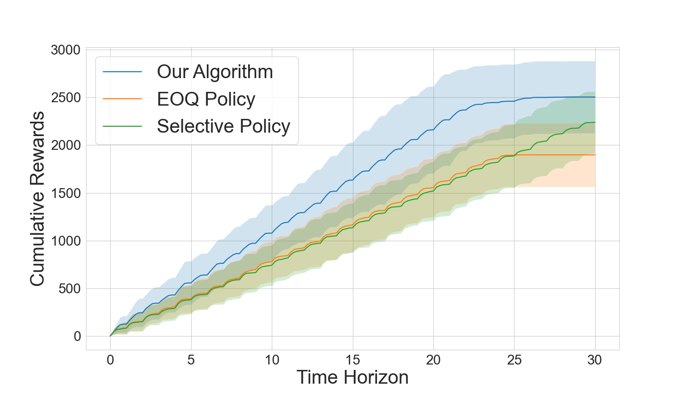
Figure 1: Reward Comparison: Algorithm vs. EOQ Policy vs. Selective Policy

Acknowledgements

This research is supported, in part, by the KAIST Starting Fund (KAIST-G04220016), the FOUR Brain Korea 21 Program (NRF-5199990113928), the National Research Foundation of Korea (NRF-2022M3J6A1063021).

Appendix A AUXILIARY MEASURES AND NOTATIONS

In this section, we define some auxiliary measures and functions that are useful for the analysis of the online dual algorithm (Algorithm 1).

Given a policy $\pi$, we define the reward-to-go function for a state $s\in\mathcal{S}$ at step $h$ with reward function $\ell:\mathcal{S}\times\mathcal{A}\times[H]\to[0,1]$ and transition kernel $P$ as follows.

$$J^{P,\pi,\ell}(s,h)=\mathbb{E}\left[\sum_{j=h}^{H}\ell\left(s_{j}^{P,\pi},a_{j}^{P,\pi},j\right)\mid\ell,\pi,P,s_{h}^{P,\pi}=s\right].$$ (8)

Similarly, we define the state-action value function for $(s,a)\in\mathcal{S}\times\mathcal{A}$ at step $h$ with reward function $\ell:\mathcal{S}\times\mathcal{A}\times[H]\to[0,1]$ and transition kernel $P$ as follows.

$$Q^{P,\pi,\ell}(s,a,h)=\mathbb{E}\left[\sum_{j=h}^{H}\ell\left(s_{j}^{P,\pi},a_{j}^{P,\pi},j\right)\mid\ell,\pi,P,s_{h}^{P,\pi}=s,a_{h}^{P,\pi}=a\right].$$ (9)

Furthermore, given a policy $\pi$ and a transition kernel $P$, we define $q^{P,\pi}\left(s,a,h\mid s^{\prime},m\right)$ as

$$q^{P,\pi}\left(s,a,h\mid s^{\prime},m\right)=\mathbb{P}\left[s^{P,\pi}_{h}=s,\ a^{P,\pi}_{h}=a\mid\pi,P,s^{P,\pi}_{m}=s^{\prime}\right]$$ (10)

for $(s,a,s^{\prime})\in\mathcal{S}\times\mathcal{A}\times\mathcal{S}$ and $1\leq m\leq h\leq H$.

Given two vectors $\bm{u},\bm{v}\in\mathbb{R}^{S\times A\times H}$, let $\bm{u}\odot\bm{v}$ be defined as the vector obtained from coordinate-wise products of $\bm{u}$ and $\bm{v}$, i.e. $(\bm{u}\odot\bm{v})_{i}=u_{i}\odot v_{i}$ for $i\in[SAH]$. Let $\vec{h}$ be an $(S\times A\times H)$-dimensional vector all of whose coordinates are $h$.

We define $\xi_{1}$ as $\xi_{1}=\left\{f_{1},g_{1}\right\}$ and for $t\geq 2$, we define $\xi_{t}$ as

$$\left\{s_{1}^{P,\pi_{t-1}},a_{1}^{P,\pi_{t-1}},\ldots,s_{h}^{P,\pi_{t-1}},a_{h}^{P,\pi_{t-1}},f_{t},g_{t}\right\}$$

where $\pi_{t-1}$ denotes the policy for episode $t-1$ and

$$\left(s_{1}^{P,\pi_{t-1}},a_{1}^{P,\pi_{t-1}},\ldots,s_{h}^{P,\pi_{t-1}},a_{h}^{P,\pi_{t-1}}\right)$$

is the trajectory generated under policy $\pi_{t-1}$ and transition kernel $P$. Then for $t\in[T]$, let $\mathcal{F}_{t}$ be defined as the $\sigma$-algebra generated by the random variables in $\xi_{1}\cup\cdots\cup\xi_{t}$. Then it follows that $\mathcal{F}_{1},\ldots,\mathcal{F}_{T}$ give rise to a filtration.

We define $\zeta_{1}$ as $\zeta_{1}=\emptyset$ and for $t\geq 2$, we define $\zeta_{t}$ as

$$\left\{f_{t-1},g_{t-1},s_{1}^{P,\pi_{t-1}},a_{1}^{P,\pi_{t-1}},\ldots,s_{h}^{P,\pi_{t-1}},a_{h}^{P,\pi_{t-1}}\right\}.$$

Then for $t\in[T]$, let $\mathcal{G}_{t}$ be defined as the $\sigma$-algebra generated by the random variables in $\zeta_{1}\cup\cdots\cup\zeta_{t}$. Then it follows that $\mathcal{G}_{1},\ldots,\mathcal{G}_{T}$ give rise to a filtration.

Appendix B MISSING PROOFS FOR SECTION 3

In this section, we first prove Lemma 3.1 which characterizes valid occupancy measures for a finite-horizon MDP. Then we prove the lemmas in Section 3.2 which describe important properties of the confidence sets estimating the true transition kernel. Lastly, we prove the lemmas in Section 3.3 which delineate the accuracy of our optimistic estimators of the mean reward function $f$ and the mean resource consumption function $g$.

B.1 Valid Occupancy Measures

First, we provide the proof of Lemma 3.1 which is based on the reduction to the loop-free MDP setting.

Proof of Lemma 3.1.

Given the finite-horizon MDP associated with transition kernel $P$, we may define a loop-free MDP as follows. We define its state space as $\mathcal{S}^{\prime}:=\mathcal{S}\times[H+1]$, which can be viewed as $H+1$ layers $\mathcal{S}\times\{h\}$ for $h\in[H+1]$. Its transition kernel $P^{\prime}$ is given by $P^{\prime}((s^{\prime},h+1)\mid(s,h),a)=P(s^{\prime}\mid s,a,h)$ for $(s,a,s^{\prime},h)\in\mathcal{S}\times\mathcal{A}\times\mathcal{S}\times[H]$. Next, given $\bar{q}$, we may define an occupancy measure $q^{\prime}$ for the loop-free MDP as $q^{\prime}((s,h),a,(s^{\prime},h+1))=\bar{q}(s,a,s^{\prime},h)$ for $(s,a,s^{\prime},h)\in\mathcal{S}\times\mathcal{A}\times\mathcal{S}\times[H]$. Then it follows from (Rosenberg and Mansour,, 2019, Lemma 3.1) that $q^{\prime}$ is a valid occupancy measure for the loop-free MDP with transition kernel $P^{\prime}$ if and only if $q^{\prime}$ satisfies

$$\sum_{(s,a,s^{\prime})\in\mathcal{S}\times\mathcal{A}\times\mathcal{S}}q^{\prime}((s,h),a,(s^{\prime},h+1))=1\quad\text{for\leavevmode\nobreak\ }h=1,\ldots,H,$$ (C1’)

$$\sum_{(s^{\prime},a)\in\mathcal{S}\times\mathcal{A}}q^{\prime}((s,h),a,(s^{\prime},h+1))=\sum_{(s^{\prime},a)\in\mathcal{S}\times\mathcal{A}}q^{\prime}((s^{\prime},h-1),a,(s,h))\quad\text{for\leavevmode\nobreak\ }s\in\mathcal{S},\ h\in\{2,\ldots,H\},$$ (C2’)

and $P^{q^{\prime}}=P^{\prime}$ where $P^{q^{\prime}}$ is given by

$$P^{q^{\prime}}((s^{\prime},h+1)\mid(s,h),a)=\frac{q^{\prime}((s,h),a,(s^{\prime},h+1))}{\sum_{s^{\prime\prime}\in\mathcal{S}}q^{\prime}((s,h),a,(s^{\prime\prime},h+1))}=\frac{\bar{q}(s,a,s^{\prime},h)}{\sum_{s^{\prime\prime}\in\mathcal{S}}\bar{q}(s,a,s^{\prime\prime},h)}.$$

Here, the conditions are equivalent to (C1), (C2), and $P^{\bar{q}}=P$. Moreover, $q^{\prime}$ is a valid occupancy measure with $P^{\prime}$ if and only if $q$ is a valid occupancy measure with $P$, as required. ∎

B.2 Confidence Sets for the True Transition Kernel

Lemma 3.2 is a modification of (Jin et al.,, 2020, Lemma 2) to our finite-horizon MDP setting. We prove Lemma 3.2 using the empirical Bernstein inequality provided in Lemma F.1.

Proof of Lemma 3.2.

We will show that with probability at least $1-4\delta$,

$$\left|P(s^{\prime}\mid s,a,h)-\bar{P}_{t}(s^{\prime}\mid s,a,h)\right|\leq\epsilon_{t}(s^{\prime}\mid s,a,h)$$ (11)

where

$$\epsilon_{t}(s^{\prime}\mid s,a,h)=2\sqrt{\frac{\bar{P}_{t}(s^{\prime}\mid s,a,h)\ln\left({{HSAT}/{\delta}}\right)}{\max\{1,N_{t}(s,a,h)-1\}}}+\frac{14\ln\left({{HSAT}/{\delta}}\right)}{3\max\{1,N_{t}(s,a,h)-1\}}$$

holds for every $(s,a,s^{\prime},h)\in\mathcal{S}\times\mathcal{A}\times\mathcal{S}\times[H]$ and every episode $t\in[T]$.

Let us first consider the case $N_{t}(s,a,h)\leq 1$. As we may assume that $HSAT\geq 2$, it follows that

$$\epsilon_{t}(s^{\prime}\mid s,a,h)=\frac{14\ln\left({{HSAT}/{\delta}}\right)}{3\max\{1,N_{t}(s,a,h)-1\}}\geq\frac{14}{3}\ln 2>1.$$

Then (11) holds because $0\leq P(s^{\prime}\mid s,a,h),\bar{P}_{t}(s^{\prime}\mid s,a,h)\leq 1$.

Assume that $n=N_{t}(s,a,h)\geq 2$. Then we define $Z_{1},\ldots,Z_{n}$ as follows.

$$Z_{j}=\begin{cases}1,\quad&\text{if the transition after the $j$th visit to $(s,a,h)$ is $s^{\prime}$},\\ 0,\quad&\text{otherwise}.\end{cases}$$

Then $Z_{1},\ldots,Z_{n}$ are i.i.d. with mean $P(s^{\prime}\mid s,a,h)$, and we have

$$\sum_{j=1}^{n}Z_{j}=M_{t}(s,a,s^{\prime},h).$$

Moreover, the sample variance $V_{n}$ of $Z_{1},\ldots,Z_{n}$ is given by

$$\begin{aligned} V_{n}&=\frac{1}{N_{t}(s,a,h)(N_{t}(s,a,h)-1)}M_{t}(s,a,s^{\prime},h)\left(N_{t}(s,a,h)-M_{t}(s,a,s^{\prime},h)\right)\\ &=\frac{N_{t}(s,a,h)}{(N_{t}(s,a,h)-1)}\bar{P}_{t}(s^{\prime}\mid s,a,h)\left(1-\bar{P}_{t}(s^{\prime}\mid s,a,h)\right).\end{aligned}$$ (12)

Then it follows from Lemma F.1 that with probability at least $1-2\delta/(HS^{2}AT)$,

$$\begin{aligned} P(s^{\prime}\mid s,a,h)-\bar{P}_{t}(s^{\prime}\mid s,a,h)&\leq\sqrt{\frac{2\bar{P}_{t}(s^{\prime}\mid s,a,h)\left(1-\bar{P}_{t}(s^{\prime}\mid s,a,h)\right)\ln\left({{HS^{2}AT}/{\delta}}\right)}{N_{t}(s,a,h)-1}}+\frac{7\ln\left(HS^{2}AT/\delta\right)}{3(N_{t}(s,a,h)-1)}.\end{aligned}$$ (13)

Here, as we assumed that $N_{t}(s,a,h)\geq 2$, we have $N_{t}(s,a,h)-1=\max\{1,N_{t}(s,a,h)-1\}$. In addition, we know that $1-\bar{P}_{t}(s^{\prime}\mid s,a,h)\leq 1$ and that $\ln\left({{HS^{2}AT}/{\delta}}\right)\leq 2\ln\left(HSAT/\delta\right)$. Then (13) implies that with probability at least $1-2\delta/(HS^{2}AT)$,

$$P(s^{\prime}\mid s,a,h)-\bar{P}_{t}(s^{\prime}\mid s,a,h)\leq\epsilon_{t}(s^{\prime}\mid s,a,h)$$ (14)

Next, we apply Lemma F.1 to variables $1-Z_{1},\ldots,1-Z_{n}$ that are i.i.d. and have mean $1-\bar{P}_{t}(s^{\prime}\mid s,a,h)$. Moreover, the sample variance of $1-Z_{1},\ldots,1-Z_{n}$ is also equal to $V_{n}$ defined as in (12). Therefore, based on the same argument, we deduce that with probability at least $1-2\delta/(HS^{2}AT)$,

$$-P(s^{\prime}\mid s,a,h)+\bar{P}_{t}(s^{\prime}\mid s,a,h)\leq\epsilon_{t}(s^{\prime}\mid s,a,h).$$ (15)

By applying union bound to (14) and (15), with probability at least $1-4\delta/(HS^{2}AT)$, (11) holds for $(s,a,s^{\prime},h)$. Furthermore, by applying union bound over all $(s,a,s^{\prime},h)\in\mathcal{S}\times\mathcal{A}\times\mathcal{S}\times[H]$, it follows that with probability at least $1-4\delta$, (11) holds for every $(s,a,s^{\prime},h)\in\mathcal{S}\times\mathcal{A}\times\mathcal{S}\times[H]$, as required. ∎

Lemma 3.2 bounds the difference between the true transition kernel $P$ and the empirical transition kernels $\bar{P}_{t}$. Based on Lemma 3.2, the next lemma bounds the difference between the true transition kernel $P$ and any $\widehat{P}$ contained in the confidence sets $\mathcal{P}_{t}$. Lemma B.1 is a modification of (Jin et al.,, 2020, Lemma 8) to our finite-horizon MDP setting.

Lemma B.1.

Let $t\in[T]$. Assume that the true transition kernel satisfies $P\in\mathcal{P}_{t}$. Then we have

$$\left|\widehat{P}(s^{\prime}\mid s,a,h)-P(s^{\prime}\mid s,a,h)\right|\leq\epsilon_{t}^{*}(s^{\prime}\mid s,a,h)$$ (16)

where

$$\epsilon_{t}^{\star}(s^{\prime}\mid s,a,h)=6\sqrt{\frac{P(s^{\prime}\mid s,a,h)\ln\left({{HSAT}/{\delta}}\right)}{\max\{1,N_{t}(s,a,h)\}}}+94\frac{\ln\left({{HSAT}/{\delta}}\right)}{\max\{1,N_{t}(s,a,h)\}}$$

for every $\widehat{P}\in\mathcal{P}_{t}$ and every $(s,a,s^{\prime},h)\in\mathcal{S}\times\mathcal{A}\times\mathcal{S}\times[H]$.

Proof.

We follow the proof of (Cohen et al.,, 2020, Lemma B.13). Note that

$$\max\{1,N_{t}(s,a,h)-1\}\geq\frac{1}{2}\cdot\max\{1,N_{t}(s,a,h)\}$$

holds for any value of $N_{t}(s,a,h)$. As we assumed that $P\in\mathcal{P}_{t}$, we have that

$$\bar{P}_{t}(s^{\prime}\mid s,a,h)\leq P(s^{\prime}\mid s,a,h)+\sqrt{\frac{8\bar{P}_{t}(s^{\prime}\mid s,a,h)\ln\left({{HSAT}/{\delta}}\right)}{\max\{1,N_{t}(s,a,h)\}}}+\frac{28\ln\left({{HSAT}/{\delta}}\right)}{3\max\{1,N_{t}(s,a,h)\}}.$$

We may view this as a quadratic inequality in terms of $x=\sqrt{\bar{P}_{t}(s^{\prime}\mid s,a,h)}$. Note that $x^{2}\leq ax+b+c$ for any $a,b,c\geq 0$ implies that $x\leq a+\sqrt{b}+\sqrt{c}$. Therefore, we deduce that

$$\sqrt{\bar{P}_{t}(s^{\prime}\mid s,a,h)} \leq\sqrt{P(s^{\prime}\mid s,a,h)}+\left(2\sqrt{2}+\sqrt{\frac{28}{3}}\right)\sqrt{\frac{\ln\left({{HSAT}/{\delta}}\right)}{\max\{1,N_{t}(s,a,h)\}}}$$

$$\leq\sqrt{P(s^{\prime}\mid s,a,h)}+13\sqrt{\frac{\ln\left({{HSAT}/{\delta}}\right)}{\max\{1,N_{t}(s,a,h)\}}}.$$

Using this bound on $\sqrt{\bar{P}_{t}(s^{\prime}\mid s,a,h)}$, we obtain the following.

$$\begin{aligned} \epsilon_{t}(s^{\prime}\mid s,a,h)&\leq\sqrt{\frac{8\bar{P}_{t}(s^{\prime}\mid s,a,h)\ln\left({{HSAT}/{\delta}}\right)}{\max\{1,N_{t}(s,a,h)\}}}+\frac{28\ln\left({{HSAT}/{\delta}}\right)}{3\max\{1,N_{t}(s,a,h)\}}\\ &\leq\sqrt{\frac{8P(s^{\prime}\mid s,a,h)\ln\left({{HSAT}/{\delta}}\right)}{\max\{1,N_{t}(s,a,h)\}}}+\left(13\sqrt{8}+\frac{28}{3}\right)\frac{\ln\left({{HSAT}/{\delta}}\right)}{\max\{1,N_{t}(s,a,h)\}}\\ &\leq 3\sqrt{\frac{P(s^{\prime}\mid s,a,h)\ln\left({{HSAT}/{\delta}}\right)}{\max\{1,N_{t}(s,a,h)\}}}+47\frac{\ln\left({{HSAT}/{\delta}}\right)}{\max\{1,N_{t}(s,a,h)\}}\\ &=\frac{1}{2}\cdot\epsilon_{t}^{\star}(s^{\prime}\mid s,a,h)\end{aligned}$$ (17)

Since we assumed that $P\in\mathcal{P}_{t}$,

$$\left|P(s^{\prime}\mid s,a,h)-\bar{P}_{t}(s^{\prime}\mid s,a,h)\right|\leq\frac{1}{2}\cdot\epsilon_{t}^{\star}(s^{\prime}\mid s,a,h).$$

Moreover, for any $\widehat{P}\in\mathcal{P}_{t}$, we have

$$\left|\widehat{P}(s^{\prime}\mid s,a,h)-\bar{P}_{t}(s^{\prime}\mid s,a,h)\right|\leq\epsilon_{t}(s^{\prime}\mid s,a,h)\leq\frac{1}{2}\cdot\epsilon_{t}^{\star}(s^{\prime}\mid s,a,h).$$

By the triangle inequality, it follows that

$$\left|\widehat{P}(s^{\prime}\mid s,a,h)-P(s^{\prime}\mid s,a,h)\right|\leq\epsilon_{t}^{\star}(s^{\prime}\mid s,a,h),$$

as required. ∎

B.3 Optimistic Function Estimators

Lemma 3.4 is a modification of (Chen and Luo,, 2021, Lemma 19) to our finite-horizon MDP setting. We prove Lemma 3.4 using the concentration inequality provided in Lemma F.4. Although we follow the same proof outline of (Chen and Luo,, 2021, Lemma 19), we provide the proof here to make our paper self-contained.

Proof of Lemma 3.4.

If $\sum_{k=1}^{t-1}\mathbbm{1}_{k}(s,a,h)=0$, then $\bar{f}_{t}(s,a,h)=\bar{g}_{t}(s,a,h)=0$ while $7R_{t}(s,a,h)\geq 7\ln 2\geq 1$, in which case we have $\widehat{f}_{t}(s,a,h)=1$ and $\widehat{g}_{t}(s,a,h)=0$. Hence, if $\sum_{k=1}^{t-1}\mathbbm{1}_{k}(s,a,h)=0$, the statements of the lemma are trivially satisfied. Thus we may assume that $\sum_{k=1}^{t-1}\mathbbm{1}_{k}(s,a,h)\geq 1$ in which case $C_{t}(s,a,h)=\sum_{k=1}^{t-1}\mathbbm{1}_{k}(s,a,h)$. Moreover, we have $C_{t}(s,a,h)\leq T$.

Applying Lemma F.4 on the first $C_{t}(s,a,h)$ realizations of the random reward for $(s,a,h)$, we deduce that

$$\left|\bar{f}_{t}(s,a,h)-f(s,a,h)\right|\leq 2\sqrt{R_{t}(s,a,h)\bar{f}_{t}(s,a,h)}+7R_{t}(s,a,h)$$ (18)

holds for every $t\in[T]$ with probability at least $1-\delta/(SAH)$. Then by taking the union bound for all $(s,a,h)\in\mathcal{S}\times\mathcal{A}\times[H]$, with probability at least $1-\delta$, (18) holds for all $(s,a,h)\in\mathcal{S}\times\mathcal{A}\times[H]$ and all $t\in[H]$. Recall that

$$\widehat{f}_{t}(s,a,h)=\min\left\{1,\bar{f}_{t}(s,a,h)+2\sqrt{R_{t}(s,a,h)\bar{f}_{t}(s,a,h)}+7R_{t}(s,a,h)\right\}.$$

This means thst

$$\widehat{f}_{t}(s,a,h)-f(s,a,h)=\widehat{f}_{t}(s,a,h)-\bar{f}_{t}(s,a,h)+\bar{f}_{t}(s,a,h)-f(s,a,h)\leq 2\left(2\sqrt{R_{t}(s,a,h)\bar{f}_{t}(s,a,h)}+7R_{t}(s,a,h)\right)$$

Since $f(s,a,h)\leq 1$, it follows that

$$0\leq\widehat{f}_{t}(s,a,h)-f(s,a,h)$$

holds if (18) holds. Furthermore, if $x\leq a\sqrt{x}+b$ holds for some $x,a,b\geq 0$, then we have $x\leq(a+\sqrt{b})^{2}$. Applying this to (18) with $x=\bar{f}_{t}(s,a,h)$, it follows that

$$\bar{f}_{t}(s,a,h)\leq f(s,a,h)+23R_{t}(s,a,h)+4\sqrt{R_{t}(s,a,h)f(s,a,h)}\leq 3f(s,a,h)+25R_{t}(s,a,h).$$

Based on this inequality, we deduce that

$$2\sqrt{R_{t}(s,a,h)\bar{f}_{t}(s,a,h)}+7R_{t}(s,a,h)\leq 4\sqrt{R_{t}(s,a,h)f(s,a,h)}+17R_{t}(s,a,h).$$

Therefore, it follows that

$$0\leq\widehat{f}_{t}(s,a,h)-f(s,a,h)\leq 8\sqrt{R_{t}(s,a,h)f(s,a,h)}+34R_{t}(s,a,h)$$

holds for all $(s,a,h,t)\in\mathcal{S}\times\mathcal{A}\times[H]\times[T]$ with probability at least $1-\delta$. as required. Likewise,

$$0\leq g(s,a,h)-\widehat{g}_{t}(s,a,h)\leq 8\sqrt{R_{t}(s,a,h)f(s,a,h)}+34R_{t}(s,a,h)$$

holds for all $(s,a,h,t)\in\mathcal{S}\times\mathcal{A}\times[H]\times[T]$ with probability at least $1-\delta$. By taking the union bound, both simultaneously hold with probability at least $1-2\delta$. ∎

Appendix C TECHNICAL LEMMAS

In this section, we prove technical lemmas that are crucial in proving the desired upper bounds on the regret. In particular, our regret analysis heavily depend on Lemmas C.1 and C.8.

Given two vectors $\bm{u},\bm{v}\in\mathbb{R}^{S\times A\times H}$, let $\bm{u}\odot\bm{v}$ be defined as the vector obtained from coordinate-wise products of $\bm{u}$ and $\bm{v}$, i.e. $(\bm{u}\odot\bm{v})_{i}=u_{i}\odot v_{i}$ for $i\in[SAH]$. Moreover, we define $\vec{h}$ as an $SAH$-dimensional vector whose coordinate for $(s,a,h)\in\mathcal{S}\times\mathcal{A}\times[H]$ is $h$. The following lemma is from (Chen and Luo,, 2021), and it is useful to bound the variance of $\langle\bm{n_{t}},\bm{f_{t}}\rangle$.

Lemma C.1.

(Chen and Luo,, 2021, Lemma 2) Let $\pi_{t}$ be any policy for episode $t$, and let $q_{t}$ denote the occupancy measure $q^{P,\pi_{t}}$. Let $\ell:\mathcal{S}\times\mathcal{A}\times[H]\to[0,1]$ be an arbitrary reward function. Then

$$\mathbb{E}\left[\langle\bm{n_{t}},\bm{\ell}\rangle^{2}\mid\ell,\pi_{t},P\right]\leq 2\langle\bm{q_{t}},\vec{h}\odot\bm{\ell}\rangle$$

where $\bm{q_{t}},\bm{n_{t}},\bm{\ell}$ are the vector representations of $q_{t},n_{t},\ell:\mathcal{S}\times\mathcal{A}\times[H]\to\mathbb{R}.$

Proof.

For ease of notation, let $\mathbb{E}_{t}\left[\cdot\right]$ denotes $\mathbb{E}\left[\cdot\mid\ell,\pi_{t},P\right]$, and let $s_{h}$ and $a_{h}$ denote $s_{h}^{P,\pi_{t}}$ and $a_{h}^{P,\pi_{t}}$, respectively for $h\in[H]$. Note that

$$\mathbb{E}_{t}\left[\langle\bm{n_{t}},\bm{\ell}\rangle^{2}\right] =\mathbb{E}_{t}\left[\left(\sum_{h=1}^{H}\sum_{(s,a)\in\mathcal{S}\times\mathcal{A}}n_{t}(s,a,h)\ell(s,a,h)\right)^{2}\right]$$

$$=\mathbb{E}_{t}\left[\left(\sum_{h=1}^{H}\ell(s_{h},a_{h},h)\right)^{2}\right]$$

$$\leq 2\mathbb{E}_{t}\left[\sum_{h=1}^{H}\ell(s_{h},a_{h},h)\left(\sum_{m=h}^{H}\ell(s_{m},a_{m},m)\right)\right]$$

$$=2\mathbb{E}_{t}\left[\sum_{h=1}^{H}\mathbb{E}_{t}\left[\ell(s_{h},a_{h},h)\left(\sum_{m=h}^{H}\ell(s_{m},a_{m},m)\right)\mid s_{h},a_{h}\right]\right]$$

$$=2\mathbb{E}_{t}\left[\sum_{h=1}^{H}\ell(s_{h},a_{h},h)\mathbb{E}_{t}\left[\sum_{m=h}^{H}\ell(s_{m},a_{m},m)\mid s_{h},a_{h}\right]\right]$$

$$=2\mathbb{E}_{t}\left[\sum_{h=1}^{H}\ell(s_{h},a_{h},h)Q^{P,\pi_{t},\ell}(s_{h},a_{h},h)\right]$$

$$=2\mathbb{E}_{t}\left[\sum_{h=1}^{H}\sum_{(s,a)\in\mathcal{S}\times\mathcal{A}}n_{t}(s,a,h)\ell(s,a,h)Q^{P,\pi_{t},\ell}(s,a,h)\right]$$

where the first inequality holds because $(\sum_{h=1}^{H}x_{h})^{2}\leq 2\sum_{h=1}^{H}x_{h}(\sum_{m=h}^{H}x_{h})$. Moreover,

$$\mathbb{E}_{t}\left[\sum_{h=1}^{H}\sum_{(s,a)\in\mathcal{S}\times\mathcal{A}}n_{t}(s,a,h)\ell(s,a,h)Q^{P,\pi_{t},\ell}(s,a,h)\right] =\sum_{h=1}^{H}\sum_{(s,a)\in\mathcal{S}\times\mathcal{A}}\ell(s,a,h)Q^{P,\pi_{t},\ell}(s,a,h)\mathbb{E}_{t}\left[n_{t}(s,a,h)\right]$$

$$=\sum_{h=1}^{H}\sum_{(s,a)\in\mathcal{S}\times\mathcal{A}}\ell(s,a,h)Q^{P,\pi_{t},\ell}(s,a,h)q_{t}(s,a,h)$$

$$=\langle\bm{q_{t}},\bm{\ell}\odot\bm{Q^{P,\pi_{t},\ell}}\rangle.$$

Therefore, it follows that

$$\mathbb{E}_{t}\left[\langle\bm{n_{t}},\bm{\ell}\rangle^{2}\right]\leq\langle\bm{q_{t}},\bm{\ell}\odot\bm{Q^{P,\pi_{t},\ell}}\rangle.$$

Next, observe that

$$\langle\bm{q_{t}},\bm{\ell}\odot\bm{Q^{P,\pi_{t},\ell}}\rangle \leq\sum_{h=1}^{H}\sum_{(s,a)\in\mathcal{S}\times\mathcal{A}}Q^{P,\pi_{t},\ell}(s,a,h)q_{t}(s,a,h)$$

$$=\sum_{h=1}^{H}\sum_{(s,a)\in\mathcal{S}\times\mathcal{A}}\pi(a\mid s,h)Q^{P,\pi_{t},\ell}(s,a,h)\left(\sum_{a^{\prime}\in\mathcal{A}}q_{t}(s,a^{\prime},h)\right)$$

$$=\sum_{h=1}^{H}\sum_{s\in\mathcal{S}}J^{P,\pi_{t},\ell}(s,h)\left(\sum_{a^{\prime}\in\mathcal{A}}q_{t}(s,a^{\prime},h)\right)$$

$$=\sum_{h=1}^{H}\sum_{s\in\mathcal{S}}\left(\sum_{m=h}^{H}\sum_{(s^{\prime},a^{\prime})\in\mathcal{S}\times\mathcal{A}}q_{t}(s^{\prime},a^{\prime},m\mid s,h)\ell(s^{\prime},a^{\prime},m)\right)\left(\sum_{a^{\prime}\in\mathcal{A}}q_{t}(s,a^{\prime},h)\right)$$

$$=\sum_{h=1}^{H}\sum_{m=h}^{H}\sum_{(s^{\prime},a^{\prime})\in\mathcal{S}\times\mathcal{A}}\sum_{s\in\mathcal{S}}q_{t}(s^{\prime},a^{\prime},m\mid s,h)\left(\sum_{a^{\prime}\in\mathcal{A}}q_{t}(s,a^{\prime},h)\right)\ell(s^{\prime},a^{\prime},m)$$

$$=\sum_{h=1}^{H}\sum_{m=h}^{H}\sum_{(s^{\prime},a^{\prime})\in\mathcal{S}\times\mathcal{A}}q_{t}(s^{\prime},a^{\prime},m)\ell(s^{\prime},a^{\prime},m)$$

$$=\sum_{h=1}^{H}\sum_{(s,a)\in\mathcal{S}\times\mathcal{A}}h\cdot q_{t}(s,a,h)\ell(s,a,h)$$

$$=\langle\bm{q_{t}},\vec{h}\odot\bm{\ell}\rangle$$

where the first inequality holds because $\ell(s,a,h)\leq 1$ for any $(s,a,h)$, the first equality holds because

$$q_{t}(s,a,h)=\pi(a\mid s,h)\sum_{a^{\prime}\in\mathcal{A}}q_{t}(s,a^{\prime},h),$$

the fifth equality follows from

$$\sum_{s\in\mathcal{S}}q_{t}(s^{\prime},a^{\prime},m\mid s,h)\left(\sum_{a^{\prime}\in\mathcal{A}}q_{t}(s,a^{\prime},h)\right)=q_{t}(s^{\prime},a^{\prime},m).$$

Therefore, we get that $\langle\bm{q_{t}},\bm{\ell}\odot\bm{Q^{P,\pi_{t},\ell}}\rangle\leq\langle\bm{q_{t}},\vec{h}\odot\bm{\ell}\rangle$, as required. ∎

The following lemma is from the first statement of (Chen and Luo,, 2021, Lemma 7) with a few modifications to adapt the proof to our setting.

Lemma C.2.

(Chen and Luo,, 2021, Lemma 7) Let $\pi$ be a policy, and let $\widetilde{P},\widehat{P}$ be two different transition kernels. We denote by $\widetilde{q}$ the occupancy measure $q^{\widetilde{P},\pi}$ associated with $\widetilde{P}$ and $\pi$, and we denote by $\widehat{q}$ the occupancy measure $q^{\widehat{P},\pi}$ associated with $\widehat{P}$ and $\pi$. Then

$$\widehat{q}(s,a,h)-\widetilde{q}(s,a,h) =\sum_{(s^{\prime},a^{\prime},s^{\prime\prime})\in\mathcal{S}\times\mathcal{A}\times\mathcal{S}}\sum_{m=1}^{h-1}\widetilde{q}(s^{\prime},a^{\prime},m)\left(\widehat{P}(s^{\prime\prime}\mid s^{\prime},a^{\prime},m)-\widetilde{P}(s^{\prime\prime}\mid s^{\prime},a^{\prime},m)\right)\widehat{q}(s,a,h\mid s^{\prime\prime},m+1).$$

Proof.

We prove the first statement by induction on $h$. When $h=1$, note that

$$\widehat{q}(s,a,h)=\widetilde{q}(s,a,h)=\pi(a\mid s,1)\cdot p(s).$$

Hence, both the left-hand side and right-hand side are equal to 0. Next assume that the equality holds with $h-1\geq 1$. Then we consider $h$. By the definition of occupancy measures,

$$\widehat{q}(s,a,h)-\widetilde{q}(s,a,h) =\pi(a\mid s,h)\sum_{(s^{\prime},a^{\prime})\in\mathcal{S}\times\mathcal{A}}(\widehat{P}(s\mid s^{\prime},a^{\prime},h-1)\widehat{q}(s^{\prime},a^{\prime},h-1)-\widetilde{P}(s\mid s^{\prime},a^{\prime},h-1)\widetilde{q}(s^{\prime},a^{\prime},h-1))$$

$$=\underbrace{\pi(a\mid s,h)\sum_{(s^{\prime},a^{\prime})\in\mathcal{S}\times\mathcal{A}}\widehat{P}(s\mid s^{\prime},a^{\prime},h-1)(\widehat{q}(s^{\prime},a^{\prime},h-1)-\widetilde{q}(s^{\prime},a^{\prime},h-1))}_{\text{Term 1}}$$

$$\qquad+\underbrace{\pi(a\mid s,h)\sum_{(s^{\prime},a^{\prime})\in\mathcal{S}\times\mathcal{A}}\widetilde{q}(s^{\prime},a^{\prime},h-1)(\widehat{P}(s\mid s^{\prime},a^{\prime},h-1)-\widetilde{P}(s\mid s^{\prime},a^{\prime},h-1))}_{\text{Term 2}}.$$

To provide an upper bound on Term 1, we use the induction hypothesis for $h-1$:

$$\widehat{q}(s^{\prime},a^{\prime},h-1)-\widetilde{q}(s^{\prime},a^{\prime},h-1)$$

$$=\sum_{(s^{\prime\prime},a^{\prime\prime},s^{\prime\prime\prime})\in\mathcal{S}\times\mathcal{A}\times\mathcal{S}}\sum_{m=1}^{h-2}\widetilde{q}(s^{\prime\prime},a^{\prime\prime},m)\left((\widehat{P}-\widetilde{P})(s^{\prime\prime\prime}\mid s^{\prime\prime},a^{\prime\prime},m)\right)\widehat{q}(s^{\prime},a^{\prime},h-1\mid s^{\prime\prime\prime},m+1)$$

where

$$(\widehat{P}-\widetilde{P})(s^{\prime\prime\prime}\mid s^{\prime\prime},a^{\prime\prime},m)=\widehat{P}(s^{\prime\prime\prime}\mid s^{\prime\prime},a^{\prime\prime},m)-\widetilde{P}(s^{\prime\prime\prime}\mid s^{\prime\prime},a^{\prime\prime},m).$$

In addition, observe that

$$\pi(a\mid s,h)\sum_{(s^{\prime},a^{\prime})\in\mathcal{S}\times\mathcal{A}}\widehat{P}(s\mid s^{\prime},a^{\prime},h-1)\widehat{q}(s^{\prime},a^{\prime},h-1\mid s^{\prime\prime\prime},m+1)=\widehat{q}(s,a,h\mid s^{\prime\prime\prime},m+1).$$

Therefore, it follows that Term 1 is equal to

$$\sum_{(s^{\prime\prime},a^{\prime\prime},s^{\prime\prime\prime})\in\mathcal{S}\times\mathcal{A}\times\mathcal{S}}\sum_{m=1}^{h-2}\widetilde{q}(s^{\prime\prime},a^{\prime\prime},m)\left((\widehat{P}-\widetilde{P})(s^{\prime\prime\prime}\mid s^{\prime\prime},a^{\prime\prime},m)\right)\widehat{q}(s,a,h\mid s^{\prime\prime\prime},m+1)$$

$$=\sum_{(s^{\prime},a^{\prime},s^{\prime\prime})\in\mathcal{S}\times\mathcal{A}\times\mathcal{S}}\sum_{m=1}^{h-2}\widetilde{q}(s^{\prime},a^{\prime},m)\left(\widehat{P}(s^{\prime\prime}\mid s^{\prime},a^{\prime},m)-\widetilde{P}(s^{\prime\prime}\mid s^{\prime},a^{\prime},m)\right)\widehat{q}(s,a,h\mid s^{\prime\prime},m+1).$$

Next, we upper bound Term 2. Note that

$$\widehat{q}(s,a,h\mid s^{\prime\prime},h)=\pi(a\mid s^{\prime\prime},h)\cdot\mathbf{1}\left[s^{\prime\prime}=s\right].$$

Then it follows that

$$\pi(a\mid s,h)(\widehat{P}(s\mid s^{\prime},a^{\prime},h-1)-\widetilde{P}(s\mid s^{\prime},a^{\prime},h-1))$$

$$=\sum_{s^{\prime\prime}\in\mathcal{S}}\mathbf{1}\left[s^{\prime\prime}=s\right]\cdot\pi(a\mid s^{\prime\prime},h)(\widehat{P}(s^{\prime\prime}\mid s^{\prime},a^{\prime},h-1)-\widetilde{P}(s^{\prime\prime}\mid s^{\prime},a^{\prime},h-1))$$

$$=\sum_{s^{\prime\prime}\in\mathcal{S}}\widehat{q}(s,a,h\mid s^{\prime\prime},h)(\widehat{P}(s^{\prime\prime}\mid s^{\prime},a^{\prime},h-1)-\widetilde{P}(s^{\prime\prime}\mid s^{\prime},a^{\prime},h-1)),$$

implying in turn that Term 2 equals

$$\sum_{(s^{\prime},a^{\prime},s^{\prime\prime})\in\mathcal{S}\times\mathcal{A}\times\mathcal{S}}\widetilde{q}(s^{\prime},a^{\prime},h-1)(\widehat{P}(s^{\prime\prime}\mid s^{\prime},a^{\prime},h-1)-\widetilde{P}(s^{\prime\prime}\mid s^{\prime},a^{\prime},h-1))\widehat{q}(s,a,h\mid s^{\prime\prime},h).$$

Adding the equivalent expression of Term 1 and that of Term 2 that we have obtained, we get the right-hand side of the statement. ∎

Based on Lemma B.1 and Lemma C.2, we show the following lemma, which is a modification of (Chen and Luo,, 2021, Lemma 7, the second statement).

Lemma C.3.

Let $\pi$ be a policy, and let $\widetilde{P},\widehat{P}$ be two different transition kernels. We denote by $\widetilde{q}$ the occupancy measure $q^{\widetilde{P},\pi}$ associated with $\widetilde{P}$ and $\pi$, and we denote by $\widehat{q}$ the occupancy measure $q^{\widehat{P},\pi}$ associated with $\widehat{P}$ and $\pi$. If $\widehat{P},\widetilde{P}\in\mathcal{P}_{t}$, then we have

$$\left|\langle\bm{\widehat{q}}-\bm{\widetilde{q}},\bm{\ell}\rangle\right| =\left|\sum_{(s,a,s^{\prime},h)\in\mathcal{S}\times\mathcal{A}\times\mathcal{S}\times[H]}\widetilde{q}(s,a,h)\left(\widehat{P}(s^{\prime}\mid s,a,h)-\widetilde{P}(s^{\prime}\mid s,a,h)\right)J^{\widehat{P},\pi,\ell}(s^{\prime},h+1)\right|$$

$$\leq H\sum_{(s,a,s^{\prime},h)\in\mathcal{S}\times\mathcal{A}\times\mathcal{S}\times[H]}\widetilde{q}(s,a,h)\epsilon_{t}^{\star}(s^{\prime}\mid s,a,h)$$

where $\bm{\widehat{q}},\bm{\widetilde{q}},\bm{\ell}$ are the vector representations of $\widehat{q},\widetilde{q},\ell:\mathcal{S}\times\mathcal{A}\times[H]\to\mathbb{R}.$

Proof.

First, observe that

$$\langle\bm{\widehat{q}}-\bm{\widetilde{q}},\bm{\ell}\rangle =\sum_{(s,a,h)\in\mathcal{S}\times\mathcal{A}\times[H]}\left(\widehat{q}(s,a,h)-\widetilde{q}(s,a,h)\right)\ell(s,a,h).$$

By Lemma C.2, the right-hand side can be rewritten so that we obtain the following.

$$\langle\bm{\widehat{q}}-\bm{\widetilde{q}},\bm{\ell}\rangle =\sum_{(s,a,h)}\sum_{(s^{\prime},a^{\prime},s^{\prime\prime})}\sum_{m=1}^{h-1}\widetilde{q}(s^{\prime},a^{\prime},m)\left((\widehat{P}-\widetilde{P})(s^{\prime\prime}\mid s^{\prime},a^{\prime},m)\right)\widehat{q}(s,a,h\mid s^{\prime\prime},m+1)\ell(s,a,h)$$

$$=\sum_{m=1}^{H}\sum_{(s^{\prime},a^{\prime},s^{\prime\prime})}\widetilde{q}(s^{\prime},a^{\prime},m)\left((\widehat{P}-\widetilde{P})(s^{\prime\prime}\mid s^{\prime},a^{\prime},m)\right)\sum_{(s,a,h):h>m}\widehat{q}(s,a,h\mid s^{\prime\prime},m+1)\ell(s,a,h)$$

$$=\sum_{m=1}^{H}\sum_{(s^{\prime},a^{\prime},s^{\prime\prime})}\widetilde{q}(s^{\prime},a^{\prime},m)\left((\widehat{P}-\widetilde{P})(s^{\prime\prime}\mid s^{\prime},a^{\prime},m)\right)J^{\widehat{P},\pi,\ell}(s^{\prime\prime},m+1)$$

$$=\sum_{h=1}^{H}\sum_{(s^{\prime},a^{\prime},s^{\prime\prime})}\widetilde{q}(s^{\prime},a^{\prime},h)\left(\widehat{P}(s^{\prime\prime}\mid s^{\prime},a^{\prime},h)-\widetilde{P}(s^{\prime\prime}\mid s^{\prime},a^{\prime},h)\right)J^{\widehat{P},\pi,\ell}(s^{\prime\prime},h+1).$$

Since $\widehat{P},P\in\mathcal{P}_{t}$, Lemma B.1 implies that

$$\left|\langle\bm{\widehat{q}}-\bm{\widetilde{q}},\bm{\ell}\rangle\right| \leq\sum_{h=1}^{H}\sum_{(s^{\prime},a^{\prime},s^{\prime\prime})}\widetilde{q}(s^{\prime},a^{\prime},h)\left|\widehat{P}(s^{\prime\prime}\mid s^{\prime},a^{\prime},h)-\widetilde{P}(s^{\prime\prime}\mid s^{\prime},a^{\prime},h)\right|J^{\widehat{P},\pi,\ell}(s^{\prime\prime},h+1)$$

$$\leq\sum_{h=1}^{H}\sum_{(s^{\prime},a^{\prime},s^{\prime\prime})}\widetilde{q}(s^{\prime},a^{\prime},h)\epsilon_{t}^{\star}(s^{\prime\prime}\mid s^{\prime},a^{\prime},h)J^{\widehat{P},\pi,\ell}(s^{\prime\prime},h+1)$$

$$\leq H\sum_{h=1}^{H}\sum_{(s^{\prime},a^{\prime},s^{\prime\prime})}\widetilde{q}(s^{\prime},a^{\prime},h)\epsilon_{t}^{\star}(s^{\prime\prime}\mid s^{\prime},a^{\prime},h)$$

$$=H\sum_{(s,a,s^{\prime},h)\in\mathcal{S}\times\mathcal{A}\times\mathcal{S}\times[H]}\widetilde{q}(s,a,h)\epsilon_{t}^{\star}(s^{\prime}\mid s,a,h)$$

where the third inequality holds because $J^{\widehat{P},\pi,\ell}(s^{\prime\prime},h+1)\leq H$, as required. ∎

Lemma C.4.

Let $\pi$ be a policy, and let $\widetilde{P},\widehat{P}$ be two different transition kernels. We denote by $\widetilde{q}$ the occupancy measure $q^{\widetilde{P},\pi}$ associated with $\widetilde{P}$ and $\pi$, and we denote by $\widehat{q}$ the occupancy measure $q^{\widehat{P},\pi}$ associated with $\widehat{P}$ and $\pi$. Let $(s,h)\in\mathcal{S}\times[H]$, and consider $\widetilde{q}(\cdot\mid s,h),\widehat{q}(\cdot\mid s,h):\mathcal{S}\times\mathcal{A}\times\{h,\ldots,H\}$. If $\widehat{P},\widetilde{P}\in\mathcal{P}_{t}$, then we have

$$\left|\langle\bm{\widehat{q}_{(s,h)}}-\bm{\widetilde{q}_{(s,h)}},\bm{\ell_{(h)}}\rangle\right|\leq H\sum_{(s^{\prime},a^{\prime},s^{\prime\prime},m)\in\mathcal{S}\times\mathcal{A}\times\mathcal{S}\times\{h,\ldots,H\}}\widetilde{q}(s^{\prime},a^{\prime},m\mid s,h)\epsilon_{t}^{\star}(s^{\prime\prime}\mid s^{\prime},a^{\prime},m)$$

where $\bm{\widehat{q}_{(s,h)}},\bm{\widetilde{q}_{(s,h)}},\bm{\ell_{(h)}}$ are the vector representations of $\widehat{q}(\cdot\mid s,h),\widetilde{q}(\cdot\mid s,h),\ell_{(h)}:\mathcal{S}\times\mathcal{A}\times\{h,\ldots,H\}\to\mathbb{R}.$

Proof.

The proof follows the same argument used to rove Lemmas C.2 and C.3. ∎

The following lemma is from (Chen and Luo,, 2021, Lemma 4) after some changes to adapt to our setting.

Lemma C.5.

(Chen and Luo,, 2021, Lemma 4) Let $\pi_{t}$ be the policy for episode $t$, and let $q_{t}$ denote the occupancy measure $q^{P,\pi_{t}}$. Let $\ell:\mathcal{S}\times\mathcal{A}\times[H]\to[0,\infty)$ be an arbitrary reward function, and define $\mathbb{V}_{t}(s,a,h)=\operatorname*{Var}_{s^{\prime}\sim P(\cdot\mid s,a,h)}\left[J^{P,\pi_{t},\ell}(s^{\prime},h+1)\right]$. Then

$$\langle\bm{q_{t}},\bm{\mathbb{V}_{t}}\rangle\leq\operatorname*{Var}\left[\langle\bm{n_{t}},\bm{\ell}\rangle\mid\ell,\pi_{t},P\right]$$

where $\bm{q_{t}},\bm{\mathbb{V}_{t}},\bm{n_{t}},\bm{\ell}$ are the vector representations of $q_{t},\mathbb{V}_{t},n_{t},\ell:\mathcal{S}\times\mathcal{A}\times[H]\to\mathbb{R}.$

Proof.

For ease of notation, let $s_{h}$ and $a_{h}$ denote $s_{h}^{P,\pi_{t}}$ and $a_{h}^{P,\pi_{t}}$, respectively for $h\in[H]$. Moreover, let $J(s,h)$ denote $J^{P,\pi_{t},\ell}(s,h)$ for $(s,h)\in\mathcal{S}\times[H]$. Note that

$$\langle\bm{n_{t}},\bm{\ell}\rangle=\sum_{(s,a,h)\mathcal{S}\times\mathcal{A}\times[H]}\ell(s,a,h)n_{t}(s,a,h)=\sum_{h=1}^{H}\ell\left(s_{h},a_{h},h\right).$$

For ease of notation, let $\mathbb{E}_{t}\left[\cdot\right]$ and $\operatorname*{Var}_{t}\left[\cdot\right]$ denote $\mathbb{E}\left[\cdot\mid\ell,\pi_{t},P\right]$ and $\operatorname*{Var}\left[\cdot\mid\ell,\pi_{t},P\right]$, respectively. Then

$$\mathbb{E}_{t}\left[\langle\bm{n_{t}},\bm{\ell}\rangle\right]=\mathbb{E}_{t}\left[\sum_{h=1}^{H}\ell\left(s_{h},a_{h},h\right)\right]=\mathbb{E}_{t}\left[\mathbb{E}\left[\sum_{h=1}^{H}\ell\left(s_{h},a_{h},h\right)\mid\ell,\pi_{t},P,s_{1}\right]\right]=\mathbb{E}_{t}\left[J(s_{1},1)\right]$$

Moreover,

$$\text{Var}_{t}\left[\langle\bm{n_{t}},\bm{\ell}\rangle\right] =\mathbb{E}_{t}\left[\left(\sum_{h=1}^{H}\ell\left(s_{h},a_{h},h\right)-\mathbb{E}_{t}\left[J(s_{1},1)\right]\right)^{2}\right]$$

$$=\mathbb{E}_{t}\left[\left(\sum_{h=1}^{H}\ell\left(s_{h},a_{h},h\right)-J(s_{1},1)+J(s_{1},1)-\mathbb{E}_{t}\left[J(s_{1},1)\right]\right)^{2}\right]$$

$$=\mathbb{E}_{t}\left[\left(\sum_{h=1}^{H}\ell\left(s_{h},a_{h},h\right)-J(s_{1},1)\right)^{2}\right]+\mathbb{E}_{t}\left[\left(J(s_{1},1)-\mathbb{E}_{t}\left[J(s_{1},1)\right]\right)^{2}\right]$$

$$\quad+2\mathbb{E}_{t}\left[\left(\sum_{h=1}^{H}\ell\left(s_{h},a_{h},h\right)-J(s_{1},1)\right)\left(J(s_{1},1)-\mathbb{E}_{t}\left[J(s_{1},1)\right]\right)\right]$$

$$\geq\mathbb{E}_{t}\left[\left(\sum_{h=1}^{H}\ell\left(s_{h},a_{h},h\right)-J(s_{1},1)\right)^{2}\right]$$

where the inequality is by $\mathbb{E}_{t}\left[J(s_{1},1)-\mathbb{E}_{t}\left[J(s_{1},1)\right]\mid s_{1}\right]=0$ and $\left(J(s_{1},1)-\mathbb{E}_{t}\left[J(s_{1},1)\right]\right)^{2}\geq 0$. Therefore,

$$\text{Var}_{t}\left[\langle\bm{n_{t}},\bm{\ell}\rangle\right] \geq\mathbb{E}_{t}\left[\left(\sum_{h=2}^{H}\ell\left(s_{h},a_{h},h\right)-J(s_{2},2)+\ell\left(s_{1},a_{1},1\right)+J(s_{2},2)-J(s_{1},1)\right)^{2}\right].$$

Note that

$$\begin{aligned} \mathbb{E}_{t}\left[\sum_{h=2}^{H}\ell\left(s_{h},a_{h},h\right)-J(s_{2},2)\mid s_{1},a_{1},s_{2}\right]&=\mathbb{E}_{t}\left[\sum_{h=2}^{H}\ell\left(s_{h},a_{h},h\right)\mid s_{2}\right]-J(s_{2},2)=0.\end{aligned}$$ (19)

Then

$$\text{Var}_{t}\left[\langle\bm{n_{t}},\bm{\ell}\rangle\right] \geq\mathbb{E}_{t}\left[\left(\sum_{h=2}^{H}\ell\left(s_{h},a_{h},h\right)-J(s_{2},2)\right)^{2}\right]+\mathbb{E}_{t}\left[\left(\ell\left(s_{1},a_{1},1\right)+J(s_{2},2)-J(s_{1},1)\right)^{2}\right]$$

$$\quad+2\mathbb{E}_{t}\left[\mathbb{E}_{t}\left[\left(\sum_{h=2}^{H}\ell\left(s_{h},a_{h},h\right)-J(s_{2},2)\right)\left(\ell\left(s_{1},a_{1},1\right)+J(s_{2},2)-J(s_{1},1)\right)\mid s_{1},a_{1},s_{2}\right]\right]$$

$$=\mathbb{E}_{t}\left[\left(\sum_{h=2}^{H}\ell\left(s_{h},a_{h},h\right)-J(s_{2},2)\right)^{2}\right]+\mathbb{E}_{t}\left[\left(\ell\left(s_{1},a_{1},1\right)+J(s_{2},2)-J(s_{1},1)\right)^{2}\right]$$

$$\quad+2\mathbb{E}_{t}\left[\left(\ell\left(s_{1},a_{1},1\right)+J(s_{2},2)-J(s_{1},1)\right)\mathbb{E}_{t}\left[\sum_{h=2}^{H}\ell\left(s_{h},a_{h},h\right)-J(s_{2},2)\mid s_{1},a_{1},s_{2}\right]\right]$$

$$=\mathbb{E}_{t}\left[\left(\sum_{h=2}^{H}\ell\left(s_{h},a_{h},h\right)-J(s_{2},2)\right)^{2}\right]+\mathbb{E}_{t}\left[\left(\ell\left(s_{1},a_{1},1\right)+J(s_{2},2)-J(s_{1},1)\right)^{2}\right]$$

where the last equality follows from (19). Here, the second term from the right-most side can be bounded from below as follows.

$$\mathbb{E}_{t}\left[\left(\ell\left(s_{1},a_{1},1\right)+J(s_{2},2)-J(s_{1},1)\right)^{2}\right]$$

$$=\mathbb{E}_{t}\left[\left(\ell\left(s_{1},a_{1},1\right)+\sum_{s^{\prime}\in\mathcal{S}}P(s^{\prime}\mid s_{1},a_{1},1)J(s^{\prime},2)-J(s_{1},1)+J(s_{2},2)-\sum_{s^{\prime}\in\mathcal{S}}P(s^{\prime}\mid s_{1},a_{1},1)J(s^{\prime},2)\right)^{2}\right]$$

$$=\mathbb{E}_{t}\left[\left(\ell\left(s_{1},a_{1},1\right)+\sum_{s^{\prime}\in\mathcal{S}}P(s^{\prime}\mid s_{1},a_{1},1)J(s^{\prime},2)-J(s_{1},1)\right)^{2}\right]$$

$$\quad+\mathbb{E}_{t}\left[\left(J(s_{2},2)-\sum_{s^{\prime}\in\mathcal{S}}P(s^{\prime}\mid s_{1},a_{1},1)J(s^{\prime},2)\right)^{2}\right]$$

$$\quad+2\mathbb{E}_{t}\left[\left(\ell\left(s_{1},a_{1},1\right)+\sum_{s^{\prime}\in\mathcal{S}}P(s^{\prime}\mid s_{1},a_{1},1)J(s^{\prime},2)-J(s_{1},1)\right)\left(J(s_{2},2)-\sum_{s^{\prime}\in\mathcal{S}}P(s^{\prime}\mid s_{1},a_{1},1)J(s^{\prime},2)\right)\right]$$

$$=\mathbb{E}_{t}\left[\left(\ell\left(s_{1},a_{1},1\right)+\sum_{s^{\prime}\in\mathcal{S}}P(s^{\prime}\mid s_{1},a_{1},1)J(s^{\prime},2)-J(s_{1},1)\right)^{2}\right]$$

$$\quad+\mathbb{E}_{t}\left[\left(J(s_{2},2)-\sum_{s^{\prime}\in\mathcal{S}}P(s^{\prime}\mid s_{1},a_{1},1)J(s^{\prime},2)\right)^{2}\right]$$

$$\geq\mathbb{E}_{t}\left[\mathbb{V}_{t}(s_{1},a_{1},1)\right]$$

where third equality holds because

$$\mathbb{E}_{t}\left[\left(\ell\left(s_{1},a_{1},1\right)+\sum_{s^{\prime}\in\mathcal{S}}P(s^{\prime}\mid s_{1},a_{1},1)J(s^{\prime},2)-J(s_{1},1)\right)\left(J(s_{2},2)-\sum_{s^{\prime}\in\mathcal{S}}P(s^{\prime}\mid s_{1},a_{1},1)J(s^{\prime},2)\right)\mid s_{1},a_{1}\right]$$

$$=\left(\ell\left(s_{1},a_{1},1\right)+\sum_{s^{\prime}\in\mathcal{S}}P(s^{\prime}\mid s_{1},a_{1},1)J(s^{\prime},2)-J(s_{1},1)\right)\mathbb{E}_{t}\left[J(s_{2},2)-\sum_{s^{\prime}\in\mathcal{S}}P(s^{\prime}\mid s_{1},a_{1},1)J(s^{\prime},2)\mid s_{1},a_{1}\right]$$

$$=\left(\ell\left(s_{1},a_{1},1\right)+\sum_{s^{\prime}\in\mathcal{S}}P(s^{\prime}\mid s_{1},a_{1},1)J(s^{\prime},2)-J(s_{1},1)\right)\times 0$$

and the last inequality holds because

$$\mathbb{E}_{t}\left[\left(J(s_{2},2)-\sum_{s^{\prime}\in\mathcal{S}}P(s^{\prime}\mid s_{1},a_{1},1)J(s^{\prime},2)\right)^{2}\right]=\mathbb{E}_{t}\left[\mathbb{V}_{t}(s_{1},a_{1},1)\right].$$

Then it follows that

$$\text{Var}_{t}\left[\langle\bm{n_{t}},\bm{\ell}\rangle\right] \geq\mathbb{E}_{t}\left[\left(\sum_{h=1}^{H}\ell\left(s_{h},a_{h},h\right)-J(s_{1},1)\right)^{2}\right]\geq\mathbb{E}_{t}\left[\left(\sum_{h=2}^{H}\ell\left(s_{h},a_{h},h\right)-J(s_{2},2)\right)^{2}\right]+\mathbb{E}_{t}\left[\mathbb{V}_{t}(s_{1},a_{1},1)\right].$$

Repeating the same argument, we deduce that

$$\text{Var}_{t}\left[\langle\bm{n_{t}},\bm{\ell}\rangle\right] \geq\sum_{h=1}^{H}\mathbb{E}_{t}\left[\mathbb{V}_{t}(s_{h},a_{h},h)\right]=\sum_{(s,a,h)\in\mathcal{S}\times\mathcal{A}\times[H]}q_{t}(s_{h},a_{h},h)\mathbb{V}_{t}(s_{h},a_{h},h)=\langle\bm{q_{t}},\bm{\mathbb{V}_{t}}\rangle,$$

as required. ∎

Next, using Lemma F.2 that states the Bernstein-type concentration inequality for a martingale difference sequence, we prove the following lemma that is useful for our analysis. Lemma C.6 is a modification of (Jin et al.,, 2020, Lemma 10) and (Chen and Luo,, 2021, Lemma 8) to our finite-horizon MDP setting.

Lemma C.6.

With probability at least $1-2\delta$, we have

$$\sum_{t=1}^{T}\sum_{(s,a,h)\in\mathcal{S}\times\mathcal{A}\times[H]}\frac{q_{t}(s,a,h)}{\max\left\{1,N_{t}(s,a,h)\right\}} =O\left(SAH\ln T+H\ln\left(H/\delta\right)\right)$$ (20)

$$\sum_{t=1}^{T}\sum_{(s,a,h)\in\mathcal{S}\times\mathcal{A}\times[H]}\frac{q_{t}(s,a,h)}{\sqrt{\max\left\{1,N_{t}(s,a,h)\right\}}} =O\left(H\sqrt{SAT}+SAH\ln T+H\ln\left(H/\delta\right)\right)$$ (21)

Proof.

Note that

$$\sum_{t=1}^{T}\sum_{(s,a)\in\mathcal{S}\times\mathcal{A}}\frac{q_{t}(s,a,h)}{\max\left\{1,N_{t}(s,a,h)\right\}}=\sum_{t=1}^{T}\sum_{(s,a)\in\mathcal{S}\times\mathcal{A}}\frac{n_{t}(s,a,h)}{\max\left\{1,N_{t}(s,a,h)\right\}}+\sum_{t=1}^{T}Y_{t}$$ (22)

where

$$Y_{t}=\sum_{(s,a)\in\mathcal{S}\times\mathcal{A}}\frac{-n_{t}(s,a,h)+q_{t}(s,a,h)}{\max\left\{1,N_{t}(s,a,h)\right\}}.$$

As $\mathbb{E}\left[n_{t}(s,a,h)\mid\pi_{t},P\right]=q_{t}(s,a,h)$ holds for every $(s,a,h)\in\mathcal{S}\times\mathcal{A}\times[H]$, we know that $Y_{1},\ldots,Y_{T}$ is a martingale difference sequence. We know that $Y_{t}\leq 1$ for each $t\in[T]$. Let $\mathbb{E}_{t}\left[\cdot\right]$ denote $\mathbb{E}\left[\cdot\mid\mathcal{F}_{t},P\right]$. Since $\pi_{t}$ is $\mathcal{F}_{t}$-measurable, we have $\mathbb{E}_{t}\left[n_{t}(s,a,h)\right]=q_{t}(s,a,h)$. Then we deduce

$$\mathbb{E}_{t}\left[Y_{t}^{2}\right] =\sum_{(s,a),(s^{\prime},a^{\prime})\in\mathcal{S}\times\mathcal{A}}\frac{\mathbb{E}_{t}\left[(n_{t}(s,a,h)-q_{t}(s,a,h))(n_{t}(s^{\prime},a^{\prime},h)-q_{t}(s^{\prime},a^{\prime},h))\right]}{\max\left\{1,N_{t}(s,a,h)\right\}\cdot\max\left\{1,N_{t}(s^{\prime},a^{\prime},h)\right\}}$$

$$=\sum_{(s,a),(s^{\prime},a^{\prime})\in\mathcal{S}\times\mathcal{A}}\frac{\mathbb{E}_{t}\left[n_{t}(s,a,h)n_{t}(s^{\prime},a^{\prime},h)-q_{t}(s,a,h)q_{t}(s^{\prime},a^{\prime},h)\right]}{\max\left\{1,N_{t}(s,a,h)\right\}\cdot\max\left\{1,N_{t}(s^{\prime},a^{\prime},h)\right\}}$$

$$\leq\sum_{(s,a),(s^{\prime},a^{\prime})\in\mathcal{S}\times\mathcal{A}}\frac{\mathbb{E}_{t}\left[n_{t}(s,a,h)n_{t}(s^{\prime},a^{\prime},h)\right]}{\max\left\{1,N_{t}(s,a,h)\right\}\cdot\max\left\{1,N_{t}(s^{\prime},a^{\prime},h)\right\}}$$

$$\leq\sum_{(s,a)\in\mathcal{S}\times\mathcal{A}}\frac{\mathbb{E}_{t}\left[n_{t}(s,a,h)\right]}{\max\left\{1,N_{t}(s,a,h)\right\}}$$

$$=\sum_{(s,a)\in\mathcal{S}\times\mathcal{A}}\frac{q_{t}(s,a,h)}{\max\left\{1,N_{t}(s,a,h)\right\}}$$

where the second equality holds because it follows from $\mathbb{E}_{t}\left[n_{t}(s,a,h)\right]=q_{t}(s,a,h)$ for $(s,a,h)\in\mathcal{S}\times\mathcal{A}\times[H]$ that

$$\mathbb{E}_{t}\left[q_{t}(s,a,h)n_{t}(s^{\prime},a^{\prime},h)\right]=\mathbb{E}_{t}\left[q_{t}(s^{\prime},a^{\prime},h)n_{t}(s,a,h)\right]=q_{t}(s,a,h)q_{t}(s^{\prime},a^{\prime},h),$$

the second inequality holds because $n_{t}(s,a,h)n_{t}(s^{\prime},a^{\prime},h)=0$ if $(s,a)\neq(s^{\prime},a^{\prime})$, and the last equality holds true because $\mathbb{E}_{t}\left[n_{t}(s,a,h)\right]=q_{t}(s,a,h)$ for any $(s,a,h)\in\mathcal{S}\times\mathcal{A}\times[H]$. Then we may apply Lemma F.2 with $\lambda=1/2$, and we deduce that with probability at least $1-\delta/H$,

$$\sum_{t=1}^{T}Y_{t}\leq\frac{1}{2}\sum_{t=1}^{T}\sum_{(s,a)\in\mathcal{S}\times\mathcal{A}}\frac{q_{t}(s,a,h)}{\max\left\{1,N_{t}(s,a,h)\right\}}+2\ln(H/\delta).$$

Plugging this inequality to (22), it follows that

$$\sum_{t=1}^{T}\sum_{(s,a)\in\mathcal{S}\times\mathcal{A}}\frac{q_{t}(s,a,h)}{\max\left\{1,N_{t}(s,a,h)\right\}}=2\sum_{t=1}^{T}\sum_{(s,a)\in\mathcal{S}\times\mathcal{A}}\frac{n_{t}(s,a,h)}{\max\left\{1,N_{t}(s,a,h)\right\}}+4\ln(H/\delta).$$

Here, the first term on the right-hand side can be bounded as follows. We have

$$\sum_{t=1}^{T}\frac{n_{t}(s,a,h)}{\max\left\{1,N_{t}(s,a,h)\right\}} =\sum_{t=1}^{T}\frac{n_{t}(s,a,h)}{\max\left\{1,N_{t+1}(s,a,h)\right\}}+\sum_{t=1}^{T}\left(\frac{n_{t}(s,a,h)}{\max\left\{1,N_{t}(s,a,h)\right\}}-\frac{n_{t}(s,a,h)}{\max\left\{1,N_{t+1}(s,a,h)\right\}}\right)$$

$$\leq\sum_{t=1}^{T}\frac{n_{t}(s,a,h)}{\max\left\{1,N_{t+1}(s,a,h)\right\}}+\sum_{t=1}^{T}\left(\frac{1}{\max\left\{1,N_{t}(s,a,h)\right\}}-\frac{1}{\max\left\{1,N_{t+1}(s,a,h)\right\}}\right)$$

$$\leq\sum_{t=1}^{T}\frac{n_{t}(s,a,h)}{\max\left\{1,N_{t+1}(s,a,h)\right\}}+1$$

$$=O(\ln T).$$

where the first inequality is due to $n_{t}(s,a,h)\leq 1$ and the last inequality holds because

$$n_{t}(s,a,h)=N_{t+1}(s,a,h)-N_{t}(s,a,h)\quad\text{and}\quad N_{T}(s,a,h)+n_{T}(s,a,h)\leq T.$$

Therefore, it follows that

$$\sum_{t=1}^{T}\sum_{(s,a)\in\mathcal{S}\times\mathcal{A}}\frac{n_{t}(s,a,h)}{\max\left\{1,N_{t}(s,a,h)\right\}}=\sum_{(s,a)\in\mathcal{S}\times\mathcal{A}}\sum_{t=1}^{T}\frac{n_{t}(s,a,h)}{\max\left\{1,N_{t}(s,a,h)\right\}}=O(SA\ln T).$$

As a result, for any fixed $h\in[H]$,

$$\sum_{t=1}^{T}\sum_{(s,a)\in\mathcal{S}\times\mathcal{A}}\frac{q_{t}(s,a,h)}{\max\left\{1,N_{t}(s,a,h)\right\}}=O\left(SA\ln T+\ln\left(H/\delta\right)\right)$$

holds with probability at least $1-\delta/H$. By union bound, (20) holds with probability at least $1-\delta$.

Next, we will show that (21) holds.

$$\sum_{t=1}^{T}\sum_{(s,a)\in\mathcal{S}\times\mathcal{A}}\frac{q_{t}(s,a,h)}{\sqrt{\max\left\{1,N_{t}(s,a,h)\right\}}}=\sum_{t=1}^{T}\sum_{(s,a)\in\mathcal{S}\times\mathcal{A}}\frac{n_{t}(s,a,h)}{\sqrt{\max\left\{1,N_{t}(s,a,h)\right\}}}+\sum_{t=1}^{T}Z_{t}$$ (23)

where

$$Z_{t}=\sum_{(s,a)\in\mathcal{S}\times\mathcal{A}}\frac{-n_{t}(s,a,h)+q_{t}(s,a,h)}{\sqrt{\max\left\{1,N_{t}(s,a,h)\right\}}}.$$

As $\mathbb{E}_{t}\left[n_{t}(s,a,h)\right]=q_{t}(s,a,h)$ holds for every $(s,a,h)\in\mathcal{S}\times\mathcal{A}\times[H]$, we know that $Z_{1},\ldots,Z_{T}$ is a martingale difference sequence. We know that $Z_{t}\leq 1$ for each $t\in[T]$. Then we deduce

$$\mathbb{E}_{t}\left[Z_{t}^{2}\right] \leq\sum_{(s,a),(s^{\prime},a^{\prime})\in\mathcal{S}\times\mathcal{A}}\frac{\mathbb{E}_{t}\left[n_{t}(s,a,h)n_{t}(s^{\prime},a^{\prime},h)\right]}{\sqrt{\max\left\{1,N_{t}(s,a,h)\right\}}\cdot\sqrt{\max\left\{1,N_{t}(s^{\prime},a^{\prime},h)\right\}}}$$

$$=\sum_{(s,a)\in\mathcal{S}\times\mathcal{A}}\frac{\mathbb{E}_{t}\left[n_{t}(s,a,h)\right]}{\max\left\{1,N_{t}(s,a,h)\right\}}$$

$$=\sum_{(s,a)\in\mathcal{S}\times\mathcal{A}}\frac{q_{t}(s,a,h)}{\max\left\{1,N_{t}(s,a,h)\right\}}$$

where the first inequality is derived by the same argument when bounding $\mathbb{E}_{t}[Y_{t}^{2}]$, the first equality holds because $n_{t}(s,a,h)n_{t}(s^{\prime},a^{\prime},h)=0$ if $(s,a)\neq(s^{\prime},a^{\prime})$, and the last equality holds true because $\mathbb{E}_{t}\left[n_{t}(s,a,h)\right]=q_{t}(s,a,h)$ for any $(s,a,h)\in\mathcal{S}\times\mathcal{A}\times[H]$. Then we may apply Lemma F.2 with $\lambda=1$, and we deduce that with probability at least $1-\delta/H$,

$$\sum_{t=1}^{T}Z_{t}\leq\sum_{t=1}^{T}\sum_{(s,a)\in\mathcal{S}\times\mathcal{A}}\frac{q_{t}(s,a,h)}{\max\left\{1,N_{t}(s,a,h)\right\}}+\ln(H/\delta).$$

Then with probability at least $1-2\delta$, (20) holds and

$$\begin{aligned} \sum_{h\in[H]}\sum_{t=1}^{T}Z_{t}&\leq\sum_{t=1}^{T}\sum_{(s,a,h)\in\mathcal{S}\times\mathcal{A}\times[H]}\frac{q_{t}(s,a,h)}{\max\left\{1,N_{t}(s,a,h)\right\}}+H\ln(H/\delta)=O(SAH\ln T+H\ln(H/\delta)).\end{aligned}$$ (24)

holds. Moreover, we have

$$\sum_{t=1}^{T}\frac{n_{t}(s,a,h)}{\sqrt{\max\left\{1,N_{t}(s,a,h)\right\}}}$$

$$=\sum_{t=1}^{T}\frac{n_{t}(s,a,h)}{\sqrt{\max\left\{1,N_{t+1}(s,a,h)\right\}}}+\sum_{t=1}^{T}\left(\frac{n_{t}(s,a,h)}{\sqrt{\max\left\{1,N_{t}(s,a,h)\right\}}}-\frac{n_{t}(s,a,h)}{\sqrt{\max\left\{1,N_{t+1}(s,a,h)\right\}}}\right)$$

$$\leq\sum_{t=1}^{T}\frac{n_{t}(s,a,h)}{\sqrt{\max\left\{1,N_{t+1}(s,a,h)\right\}}}+\sum_{t=1}^{T}\left(\frac{1}{\sqrt{\max\left\{1,N_{t}(s,a,h)\right\}}}-\frac{1}{\sqrt{\max\left\{1,N_{t+1}(s,a,h)\right\}}}\right)$$

$$\leq\sum_{t=1}^{T}\frac{n_{t}(s,a,h)}{\sqrt{\max\left\{1,N_{t+1}(s,a,h)\right\}}}+1$$

$$=O(\sqrt{N_{T+1}(s,a,h)}+1).$$

where the last equality holds because $n_{t}(s,a,h)=N_{t+1}(s,a,h)-N_{t}(s,a,h)$. Then

$$\sum_{t=1}^{T}\sum_{(s,a,h)\in\mathcal{S}\times\mathcal{A}\times[H]}\frac{n_{t}(s,a,h)}{\sqrt{\max\left\{1,N_{t}(s,a,h)\right\}}} =O\left(\sum_{\mathcal{S}\times\mathcal{A}\times[H]}\left(\sqrt{N_{T+1}(s,a,h)}+1\right)\right)$$

$$=O\left(\sqrt{SAH\sum_{\mathcal{S}\times\mathcal{A}\times[H]}N_{T+1}(s,a,h)}+SAH\right)$$

$$=O\left(H\sqrt{SAT}+SAH\right)$$

where the second equality is due to the Cauchy-Schwarz inequality. Then it follows from (23) and (24) that (21) holds. ∎

Lemma C.7.

Assume that $P\in\mathcal{P}_{t}$ for every episode $t\in[T]$. Then

$$\sum_{t=1}^{T}\left|\sum_{(s,a,s^{\prime},h)}q_{t}(s,a,h)\left(\left(P-P_{t}\right)(s^{\prime}\mid s,a,h)\right)\left(\left(J^{P_{t},\pi_{t},\ell}-J^{P,\pi_{t},\ell}\right)(s^{\prime},h+1)\right)\right|=O\left(H^{2}S^{2}A\left(\ln(HSAT/\delta)\right)^{2}\right)$$

for any $P_{t}\in\mathcal{P}_{t}$ where $\left(P-P_{t}\right)(s^{\prime}\mid s,a,h)=P(s^{\prime}\mid s,a,h)-P_{t}(s^{\prime}\mid s,a,h)$ and $\left(J^{P_{t},\pi_{t},\ell}-J^{P,\pi_{t},\ell}\right)(s^{\prime},h+1)=J^{P_{t},\pi_{t},\ell}(s^{\prime},h+1)-J^{P,\pi_{t},\ell}(s^{\prime},h+1)$.

Proof.

Let $\bm{q^{P_{t},\pi_{t}}_{(s^{\prime},h+1)}},\bm{q^{P,\pi_{t}}_{(s^{\prime},h+1)}},\bm{\ell}$ be the vector representations of $q^{P_{t},\pi_{t}}(\cdot\mid s^{\prime},h+1),q^{P,\pi_{t}}(\cdot\mid s^{\prime},h+1),\ell:\mathcal{S}\times\mathcal{A}\times\mathcal{S}\to[0,1]$, respectively. Note that

$$\sum_{t=1}^{T}\left|\sum_{(s,a,s^{\prime},h)}q_{t}(s,a,h)\left(\left(P-P_{t}\right)(s^{\prime}\mid s,a,h)\right)\left(\left(J^{P_{t},\pi_{t},\ell}-J^{P,\pi_{t},\ell}\right)(s^{\prime},h+1)\right)\right|$$

$$\leq\sum_{t=1}^{T}\sum_{(s,a,s^{\prime},h)}q_{t}(s,a,h)\epsilon_{t}^{\star}(s^{\prime}\mid s,a,h)\left|\left(J^{P_{t},\pi_{t},\ell}-J^{P,\pi_{t},\ell}\right)(s^{\prime},h+1)\right|$$

$$=\sum_{t=1}^{T}\sum_{(s,a,s^{\prime},h)}q_{t}(s,a,h)\epsilon_{t}^{\star}(s^{\prime}\mid s,a,h)\left|\langle\bm{q^{P_{t},\pi_{t}}_{(s^{\prime},h+1)}}-\bm{q^{P,\pi_{t}}_{(s^{\prime},h+1)}},\bm{\ell}\rangle\right|$$

$$\leq H\sum_{t=1}^{T}\sum_{(s,a,s^{\prime},h)}q_{t}(s,a,h)\epsilon_{t}^{\star}(s^{\prime}\mid s,a,h)\sum_{(s^{\prime\prime},a^{\prime\prime},s^{\prime\prime\prime}),m\geq h}q_{t}(s^{\prime\prime},a^{\prime\prime},m\mid s^{\prime},h+1)\epsilon_{t}^{\star}(s^{\prime\prime\prime}\mid s^{\prime\prime},a^{\prime\prime},m)$$

where the first inequality is from Lemma B.1, the first equality holds because $J^{P_{t},\pi_{t},\ell}(s^{\prime},h+1)=\langle\bm{q^{P_{t},\pi_{t}}_{(s^{\prime},h+1)}},\bm{\ell}\rangle$ and $J^{P,\pi_{t},\ell}(s^{\prime},h+1)=\langle\bm{q^{P,\pi_{t}}_{(s^{\prime},h+1)}},\bm{\ell}\rangle$, the second inequality is due to Lemma C.4. Then plugging in the definition of $\epsilon_{t}^{*}$, it follows that

$$\frac{1}{H\ln(HSAT/\delta)}\sum_{t=1}^{T}\left|\sum_{(s,a,s^{\prime},h)}q_{t}(s,a,h)\left(\left(P-P_{t}\right)(s^{\prime}\mid s,a,h)\right)\left(\left(J^{P_{t},\pi_{t},\ell}-J^{P,\pi_{t},\ell}\right)(s^{\prime},h+1)\right)\right|$$

$$=O\left(\sum_{\begin{subarray}{c}t,(s,a,s^{\prime},h)\\ (s^{\prime\prime},a^{\prime\prime},s^{\prime\prime\prime})\\ m\geq h+1\end{subarray}}q_{t}(s,a,h)\sqrt{\frac{P(s^{\prime}\mid s,a,h)}{\max\{1,n_{t}(s,a,h)\}}}q_{t}(s^{\prime\prime},a^{\prime\prime},m\mid s^{\prime},h+1)\sqrt{\frac{P(s^{\prime\prime\prime}\mid s^{\prime\prime},a^{\prime\prime},m)}{\max\{1,n_{t}(s^{\prime\prime},a^{\prime\prime},m)\}}}\right)$$

$$=O\left(\sum_{\begin{subarray}{c}t,(s,a,s^{\prime},h)\\ (s^{\prime\prime},a^{\prime\prime},s^{\prime\prime\prime})\\ m\geq h+1\end{subarray}}\sqrt{{\scriptstyle\frac{q_{t}(s,a,h)P(s^{\prime\prime\prime}\mid s^{\prime\prime},a^{\prime\prime},m)q_{t}(s^{\prime\prime},a^{\prime\prime},m\mid s^{\prime},h+1)}{\max\{1,n_{t}(s,a,h)\}}}}\sqrt{{\scriptstyle\frac{q_{t}(s,a,h)P(s^{\prime}\mid s,a,h)q_{t}(s^{\prime\prime},a^{\prime\prime},m\mid s^{\prime},h+1)}{\max\{1,n_{t}(s^{\prime\prime},a^{\prime\prime},m)\}}}}\right)$$

$$=O\left(\sqrt{\sum_{\begin{subarray}{c}t,(s,a,s^{\prime},h)\\ (s^{\prime\prime},a^{\prime\prime},s^{\prime\prime\prime})\\ m\geq h+1\end{subarray}}{\scriptstyle\frac{q_{t}(s,a,h)P(s^{\prime\prime\prime}\mid s^{\prime\prime},a^{\prime\prime},m)q_{t}(s^{\prime\prime},a^{\prime\prime},m\mid s^{\prime},h+1)}{\max\{1,n_{t}(s,a,h)\}}}}\sqrt{\sum_{\begin{subarray}{c}t,(s,a,s^{\prime},h)\\ (s^{\prime\prime},a^{\prime\prime},s^{\prime\prime\prime})\\ m\geq h+1\end{subarray}}{\scriptstyle\frac{q_{t}(s,a,h)P(s^{\prime}\mid s,a,h)q_{t}(s^{\prime\prime},a^{\prime\prime},m\mid s^{\prime},h+1)}{\max\{1,n_{t}(s^{\prime\prime},a^{\prime\prime},m)\}}}}\right)$$

$$=O\left(\sqrt{S\sum_{t=1}^{T}\sum_{(s,a,h)}{\frac{q_{t}(s,a,h)}{\max\{1,n_{t}(s,a,h)\}}}}\sqrt{S\sum_{t=1}^{T}\sum_{(s^{\prime\prime},a^{\prime\prime},m)}{\frac{q_{t}(s^{\prime\prime},a^{\prime\prime},m)}{\max\{1,n_{t}(s^{\prime\prime},a^{\prime\prime},m)\}}}}\right)$$

$$=O\left(S^{2}AH\ln T+SH\ln\left(H/\delta\right)\right)$$

where the third equality follows from the Cauchy-Schwarz inequality and the last equality is due to Lemma C.6. Therefore, we deduce that

$$\sum_{t=1}^{T}\left|\sum_{(s,a,s^{\prime},h)}q_{t}(s,a,h)\left(\left(P-P_{t}\right)(s^{\prime}\mid s,a,h)\right)\left(\left(J^{P_{t},\pi_{t},\ell}-J^{P,\pi_{t},\ell}\right)(s^{\prime},h+1)\right)\right|$$

$$=O\left(H^{2}S^{2}A\ln T\ln(HSAT/\delta)+SH^{2}\ln\left(H/\delta\right)\ln(HSAT/\delta)\right)$$

$$=O\left(H^{2}S^{2}A\left(\ln(HSAT/\delta)\right)^{2}\right),$$

as required. ∎

Next, we provide Lemma C.8, which is a modification of (Chen and Luo,, 2021, Lemma 9) to our finite-horizon MDP setting.

Lemma C.8.

Let $\pi_{t}$ be any policy for episode $t$, and let $P_{t}$ be any transition kernel from $\mathcal{P}_{t}$. Let $q_{t},\widehat{q}_{t}$ denote the occupancy measures $q^{P,\pi_{t}},q^{P_{t},\pi_{t}}$, respectively. Let $\ell_{t}:\mathcal{S}\times\mathcal{A}\times[H]\to[0,1]$ be an arbitrary reward function for episode $t\in[T]$. Then with probability at least $1-4\delta$,

$$\sum_{t=1}^{T}\left|\langle\bm{\ell_{t}},\bm{q_{t}}-\bm{\widehat{q}_{t}}\rangle\right|=O\left(\left(\sqrt{HS^{2}A\left(\sum_{t=1}^{T}\langle\bm{q_{t}},\vec{h}\odot\bm{\ell_{t}}\rangle+H^{3}\sqrt{T}\right)}+H^{2}S^{2}A\right)\left(\ln\frac{HSAT}{\delta}\right)^{2}\right).$$

Proof.

We define $\xi_{1}$ as $\xi_{1}=\left\{\ell_{1},\pi_{1}\right\}$ and for $t\geq 2$, we define $\xi_{t}$ as

$$\left\{s_{1}^{P,\pi_{t-1}},a_{1}^{P,\pi_{t-1}},\ldots,s_{h}^{P,\pi_{t-1}},a_{h}^{P,\pi_{t-1}},\ell_{t},\pi_{t}\right\}$$

where $\pi_{t-1}$ and $\pi_{t}$ denote the policies for episode $t-1$ and episode $t$, respectively, and

$$\left(s_{1}^{P,\pi_{t-1}},a_{1}^{P,\pi_{t-1}},\ldots,s_{h}^{P,\pi_{t-1}},a_{h}^{P,\pi_{t-1}}\right)$$

is the trajectory generated under policy $\pi_{t-1}$ and transition kernel $P$. Then for $t\in[T]$, let $\mathcal{H}_{t}$ be defined as the $\sigma$-algebra generated by the random variables in $\xi_{1}\cup\cdots\cup\xi_{t}$. Then it follows that $\mathcal{H}_{1},\ldots,\mathcal{H}_{T}$ give rise to a filtration.

Let us define

$$\mu_{t}(s,a,h)=\mathbb{E}_{s^{\prime}\sim P(\cdot\mid s,a,h)}\left[J^{P,\pi_{t},\ell_{t}}(s^{\prime},h+1)\right].$$

Note that

$$\sum_{t=1}^{T}\left|\langle\bm{q_{t}}-\bm{\widehat{q}_{t}},\bm{\ell_{t}}\rangle\right| =\sum_{t=1}^{T}\left|\sum_{(s,a,s^{\prime},h)\in\mathcal{S}\times\mathcal{A}\times\mathcal{S}\times[H]}q_{t}(s,a,h)\left(P(s^{\prime}\mid s,a,h)-P_{t}(s^{\prime}\mid s,a,h)\right)J^{P_{t},\pi_{t},\ell_{t}}(s^{\prime},h+1)\right|$$

$$\leq\sum_{t=1}^{T}\left|\sum_{(s,a,s^{\prime},h)\in\mathcal{S}\times\mathcal{A}\times\mathcal{S}\times[H]}q_{t}(s,a,h)\left(P(s^{\prime}\mid s,a,h)-P_{t}(s^{\prime}\mid s,a,h)\right)J^{P,\pi_{t},\ell_{t}}(s^{\prime},h+1)\right|$$

$$\quad+O\left(H^{2}S^{2}A\left(\ln(HSAT/\delta)\right)^{2}\right)$$

where the first equality is due to Lemma C.2 and the first inequality is by Lemma C.7. Moreover,

$$\sum_{t=1}^{T}\left|\sum_{(s,a,s^{\prime},h)\in\mathcal{S}\times\mathcal{A}\times\mathcal{S}\times[H]}q_{t}(s,a,h)\left(P(s^{\prime}\mid s,a,h)-P_{t}(s^{\prime}\mid s,a,h)\right)J^{P,\pi_{t},\ell_{t}}(s^{\prime},h+1)\right|$$

$$=\sum_{t=1}^{T}\left|\sum_{(s,a,s^{\prime},h)\in\mathcal{S}\times\mathcal{A}\times\mathcal{S}\times[H]}q_{t}(s,a,h)\left(\left(P-P_{t}\right)(s^{\prime}\mid s,a,h)\right)\left(J^{P,\pi_{t},\ell_{t}}(s^{\prime},h+1)-\mu_{t}(s,a,h)\right)\right|$$

$$\leq\sum_{t=1}^{T}\sum_{(s,a,s^{\prime},h)\in\mathcal{S}\times\mathcal{A}\times\mathcal{S}\times[H]}q_{t}(s,a,h)\epsilon_{t}^{\star}(s^{\prime}\mid s,a,h)\left|J^{P,\pi_{t},\ell_{t}}(s^{\prime},h+1)-\mu_{t}(s,a,h)\right|$$

$$\leq O\left(\sum_{t=1}^{T}\sum_{\begin{subarray}{c}(s,a,s^{\prime},h)\in\\ \mathcal{S}\times\mathcal{A}\times\mathcal{S}\times[H]\end{subarray}}q_{t}(s,a,h)\sqrt{\frac{P(s^{\prime}\mid s,a,h)\ln(HSAT/\delta)}{\max\{1,N_{t}(s,a,h)\}}\left(J^{P,\pi_{t},\ell_{t}}(s^{\prime},h+1)-\mu_{t}(s,a,h)\right)^{2}}\right)$$

$$\quad+O\left(HS\sum_{t=1}^{T}\sum_{(s,a,h)\in\mathcal{S}\times\mathcal{A}\times[H]}\frac{q_{t}(s,a,h)\ln(HSAT/\delta)}{\max\{1,N_{t}(s,a,h)\}}\right)$$

$$\leq O\left(\sum_{t=1}^{T}\sum_{\begin{subarray}{c}(s,a,s^{\prime},h)\in\\ \mathcal{S}\times\mathcal{A}\times\mathcal{S}\times[H]\end{subarray}}q_{t}(s,a,h)\sqrt{\frac{P(s^{\prime}\mid s,a,h)\ln(HSAT/\delta)}{\max\{1,N_{t}(s,a,h)\}}\left(J^{P,\pi_{t},\ell_{t}}(s^{\prime},h+1)-\mu_{t}(s,a,h)\right)^{2}}\right)$$

$$\quad+O\left(H^{2}S^{2}A\left(\ln(HSAT/\delta)\right)^{2}\right)$$

where $\left(P-P_{t}\right)(s^{\prime}\mid s,a,h)=P(s^{\prime}\mid s,a,h)-P_{t}(s^{\prime}\mid s,a,h)$, the first equality holds because $\sum_{s^{\prime}\in\mathcal{S}}\left(P-P_{t}\right)(s^{\prime}\mid s,a,h)=0$ and $\mu_{t}(s,a,h)$ is independent of $s^{\prime}$, the first inequality is due to Lemma B.1, and the second inequality is from Lemma B.1 and $\left|J^{P,\pi_{t},\ell_{t}}(s^{\prime},h+1)-\mu_{t}(s,a,h)\right|\leq H$. Recall that $q_{t}(s,a,h)=\mathbb{E}\left[n_{t}(s,a,h)\mid\pi_{t},P\right]$, which implies that

$$\sum_{t=1}^{T}\sum_{\begin{subarray}{c}(s,a,s^{\prime},h)\in\\ \mathcal{S}\times\mathcal{A}\times\mathcal{S}\times[H]\end{subarray}}q_{t}(s,a,h)\sqrt{\frac{P(s^{\prime}\mid s,a,h)\ln(HSAT/\delta)}{\max\{1,N_{t}(s,a,h)\}}\left(J^{P,\pi_{t},\ell_{t}}(s^{\prime},h+1)-\mu_{t}(s,a,h)\right)^{2}}=\sum_{t=1}^{T}\mathbb{E}\left[X_{t}\mid\mathcal{H}_{t},P\right]$$

where

$$X_{t}=\sum_{\begin{subarray}{c}(s,a,s^{\prime},h)\in\\ \mathcal{S}\times\mathcal{A}\times\mathcal{S}\times[H]\end{subarray}}n_{t}(s,a,h)\sqrt{\frac{P(s^{\prime}\mid s,a,h)\ln(HSAT/\delta)}{\max\{1,N_{t}(s,a,h)\}}\left(J^{P,\pi_{t},\ell_{t}}(s^{\prime},h+1)-\mu_{t}(s,a,h)\right)^{2}}.$$

Here, we have

$$0\leq X_{t}\leq O\left(HS\sum_{(s,a,h)\in\mathcal{S}\times\mathcal{A}\times[H]}n_{t}(s,a,h)\sqrt{\ln(HSAT/\delta)}\right)=O(H^{2}S\sqrt{\ln(HSAT/\delta)}).$$

Then it follows from Lemma F.5 that with probability at least $1-\delta$,

$$\sum_{t=1}^{T}\mathbb{E}\left[X_{t}\mid\mathcal{H}_{t},P\right]$$

$$\leq 2\sum_{t=1}^{T}\sum_{\begin{subarray}{c}(s,a,s^{\prime},h)\in\\ \mathcal{S}\times\mathcal{A}\times\mathcal{S}\times[H]\end{subarray}}n_{t}(s,a,h)\sqrt{\frac{P(s^{\prime}\mid s,a,h)\ln(HSAT/\delta)}{\max\{1,N_{t}(s,a,h)\}}\left(J^{P,\pi_{t},\ell_{t}}(s^{\prime},h+1)-\mu_{t}(s,a,h)\right)^{2}}$$

$$\quad+O\left(H^{2}S\left(\ln(HSAT/\delta)\right)^{3/2}\right).$$

Note that

$$\sum_{t=1}^{T}\sum_{\begin{subarray}{c}(s,a,s^{\prime},h)\in\\ \mathcal{S}\times\mathcal{A}\times\mathcal{S}\times[H]\end{subarray}}n_{t}(s,a,h)\sqrt{\frac{P(s^{\prime}\mid s,a,h)\ln(HSAT/\delta)}{\max\{1,N_{t}(s,a,h)\}}\left(J^{P,\pi_{t},\ell_{t}}(s^{\prime},h+1)-\mu_{t}(s,a,h)\right)^{2}}$$

$$\leq\sum_{t=1}^{T}\sum_{\begin{subarray}{c}(s,a,s^{\prime},h)\in\\ \mathcal{S}\times\mathcal{A}\times\mathcal{S}\times[H]\end{subarray}}n_{t}(s,a,h)\sqrt{\frac{P(s^{\prime}\mid s,a,h)\ln(HSAT/\delta)}{\max\{1,N_{t+1}(s,a,h)\}}\left(J^{P,\pi_{t},\ell_{t}}(s^{\prime},h+1)-\mu_{t}(s,a,h)\right)^{2}}$$

$$\quad+H\sum_{t=1}^{T}\sum_{\begin{subarray}{c}(s,a,s^{\prime},h)\in\\ \mathcal{S}\times\mathcal{A}\times\mathcal{S}\times[H]\end{subarray}}n_{t}(s,a,h)\left(\sqrt{\frac{P(s^{\prime}\mid s,a,h)\ln(HSAT/\delta)}{\max\{1,N_{t}(s,a,h)\}}}-\sqrt{\frac{P(s^{\prime}\mid s,a,h)\ln(HSAT/\delta)}{\max\{1,N_{t+1}(s,a,h)\}}}\right)$$

$$\leq\sum_{t=1}^{T}\sum_{\begin{subarray}{c}(s,a,s^{\prime},h)\in\\ \mathcal{S}\times\mathcal{A}\times\mathcal{S}\times[H]\end{subarray}}n_{t}(s,a,h)\sqrt{\frac{P(s^{\prime}\mid s,a,h)\ln(HSAT/\delta)}{\max\{1,N_{t+1}(s,a,h)\}}\left(J^{P,\pi_{t},\ell_{t}}(s^{\prime},h+1)-\mu_{t}(s,a,h)\right)^{2}}$$

$$\quad+H\sqrt{S}\sum_{t=1}^{T}\sum_{{(s,a,h)\in\mathcal{S}\times\mathcal{A}\times[H]}}\left(\sqrt{\frac{\ln(HSAT/\delta)}{\max\{1,N_{t}(s,a,h)\}}}-\sqrt{\frac{\ln(HSAT/\delta)}{\max\{1,N_{t+1}(s,a,h)\}}}\right)$$

$$\leq\sum_{t=1}^{T}\sum_{\begin{subarray}{c}(s,a,s^{\prime},h)\in\\ \mathcal{S}\times\mathcal{A}\times\mathcal{S}\times[H]\end{subarray}}n_{t}(s,a,h)\sqrt{\frac{P(s^{\prime}\mid s,a,h)\ln(HSAT/\delta)}{\max\{1,N_{t+1}(s,a,h)\}}\left(J^{P,\pi_{t},\ell_{t}}(s^{\prime},h+1)-\mu_{t}(s,a,h)\right)^{2}}$$

$$\quad+O\left(H^{2}S^{3/2}A\sqrt{\ln(HSAT/\delta)}\right).$$

where the first inequality holds because $\left|J^{P,\pi_{t},\ell_{t}}(s^{\prime},h+1)-\mu_{t}(s,a,h)\right|\leq H$, the second inequality holds because $n_{t}(s,a,h)\leq 1$ and the Cauchy-Schwarz inequality implies that

$$\sum_{s^{\prime}\in\mathcal{S}}\sqrt{P(s^{\prime}\mid s,a,h)}\leq\sqrt{S\sum_{s^{\prime}\in\mathcal{S}}P(s^{\prime}\mid s,a,h)}=\sqrt{S},$$

and the third inequality follows from

$$\sum_{t=1}^{T}\left(\sqrt{\frac{1}{\max\{1,N_{t}(s,a,h)\}}}-\sqrt{\frac{1}{\max\{1,N_{t+1}(s,a,h)\}}}\right)\leq\sqrt{\frac{1}{\max\{1,N_{1}(s,a,h)\}}}=1.$$

Next, the Cauchy-Schwarz inequality implies the following.

$$\sum_{t=1}^{T}\sum_{\begin{subarray}{c}(s,a,s^{\prime},h)\in\\ \mathcal{S}\times\mathcal{A}\times\mathcal{S}\times[H]\end{subarray}}n_{t}(s,a,h)\sqrt{\frac{P(s^{\prime}\mid s,a,h)\ln(HSAT/\delta)}{\max\{1,N_{t+1}(s,a,h)\}}\left(J^{P,\pi_{t},\ell_{t}}(s^{\prime},h+1)-\mu_{t}(s,a,h)\right)^{2}}$$

$$\leq\sqrt{\sum_{t=1}^{T}\sum_{\begin{subarray}{c}(s,a,s^{\prime},h)\in\\ \mathcal{S}\times\mathcal{A}\times\mathcal{S}\times[H]\end{subarray}}n_{t}(s,a,h){P(s^{\prime}\mid s,a,h)}\left(J^{P,\pi_{t},\ell_{t}}(s^{\prime},h+1)-\mu_{t}(s,a,h)\right)^{2}}$$

$$\quad\times\sqrt{\sum_{t=1}^{T}\sum_{\begin{subarray}{c}(s,a,s^{\prime},h)\in\\ \mathcal{S}\times\mathcal{A}\times\mathcal{S}\times[H]\end{subarray}}n_{t}(s,a,h)\frac{\ln(HSAT/\delta)}{\max\{1,N_{t+1}(s,a,h)\}}}$$

Here, the second term can be bounded as follows.

$$\sum_{t=1}^{T}\sum_{\begin{subarray}{c}(s,a,s^{\prime},h)\in\mathcal{S}\times\mathcal{A}\times\mathcal{S}\times[H]\end{subarray}}n_{t}(s,a,h)\frac{\ln(HSAT/\delta)}{\max\{1,N_{t+1}(s,a,h)\}}$$

$$=S\ln\left(\frac{HSAT}{\delta}\right)\sum_{t=1}^{T}\sum_{\begin{subarray}{c}(s,a,h)\in\mathcal{S}\times\mathcal{A}\times[H]\end{subarray}}\frac{n_{t}(s,a,h)}{\max\{1,N_{t+1}(s,a,h)\}}$$

$$=S\ln\left(\frac{HSAT}{\delta}\right)\sum_{\begin{subarray}{c}(s,a,h)\in\mathcal{S}\times\mathcal{A}\times[H]\end{subarray}}\sum_{t=1}^{T}\frac{n_{t}(s,a,h)}{\max\{1,N_{t+1}(s,a,h)\}}$$

$$=O\left(HS^{2}A\left(\ln\left({HSAT}/{\delta}\right)\right)^{2}\right).$$

$(s,a,h)\in\mathcal{S}\times\mathcal{A}\times[H]$, we define

$$\mathbb{V}_{t}(s,a,h)=\operatorname*{Var}_{s^{\prime}\sim P(\cdot\mid s,a,h)}\left[J^{P,\pi_{t},\ell_{t}}(s^{\prime},h+1)\right].$$

Then

$$\mathbb{V}_{t}(s,a,h) =\mathbb{E}_{s^{\prime}\sim P(\cdot\mid s,a,h)}\left[\left(J^{P,\pi_{t},\ell_{t}}(s^{\prime},h+1)-\mu_{t}(s,a,h)\right)^{2}\right]$$

$$=\sum_{s^{\prime}\in\mathcal{S}}P(s^{\prime}\mid s,a,h)\left(J^{P,\pi_{t},\ell_{t}}(s^{\prime},h+1)-\mu_{t}(s,a,h)\right)^{2}$$

Furthermore,

$$\sum_{t=1}^{T}\sum_{\begin{subarray}{c}(s,a,s^{\prime},h)\in\\ \mathcal{S}\times\mathcal{A}\times\mathcal{S}\times[H]\end{subarray}}n_{t}(s,a,h){P(s^{\prime}\mid s,a,h)}\left(J^{P,\pi_{t},\ell_{t}}(s^{\prime},h+1)-\mu_{t}(s,a,h)\right)^{2}$$

$$=\sum_{t=1}^{T}\sum_{\begin{subarray}{c}(s,a,h)\in\mathcal{S}\times\mathcal{A}\times[H]\end{subarray}}n_{t}(s,a,h)\mathbb{V}_{t}(s,a,h)$$

$$=\sum_{t=1}^{T}\langle\bm{q_{t}},\bm{\mathbb{V}_{t}}\rangle+\sum_{t=1}^{T}\sum_{\begin{subarray}{c}(s,a,h)\in\mathcal{S}\times\mathcal{A}\times[H]\end{subarray}}(n_{t}(s,a,h)-q_{t}(s,a,h))\mathbb{V}_{t}(s,a,h)$$

$$\leq\sum_{t=1}^{T}\operatorname*{Var}\left[\langle n_{t},\ell_{t}\rangle\mid\ell_{t},\pi_{t},P\right]+O\left(H^{3}\sqrt{T\ln(1/\delta)}\right)$$

where $\bm{\mathbb{V}_{t}}\in\mathbb{R}^{SAH}$ is the vector representation of $\mathbb{V}_{t}$ and the inequality follows from Lemma C.5, $\mathbb{V}_{t}(s,a,h)\leq H^{2}$,

$$\sum_{\begin{subarray}{c}(s,a,h)\in\mathcal{S}\times\mathcal{A}\times[H]\end{subarray}}(n_{t}(s,a,h)-q_{t}(s,a,h))\mathbb{V}_{t}(s,a,h) \leq\sum_{\begin{subarray}{c}(s,a,h)\in\mathcal{S}\times\mathcal{A}\times[H]\end{subarray}}(n_{t}(s,a,h)+q_{t}(s,a,h))H^{2}\leq 2H^{3},$$

and Lemma F.3. Therefore, we finally have proved that

$$\sum_{t=1}^{T}\left|\langle\bm{q_{t}}-\bm{\widehat{q}_{t}},\bm{\ell_{t}}\rangle\right| =O\left(\sqrt{HS^{2}A\left(\ln\frac{HSAT}{\delta}\right)^{2}\left(\sum_{t=1}^{T}\operatorname*{Var}\left[\langle n_{t},\ell_{t}\rangle\mid\ell_{t},\pi_{t},P\right]+H^{3}\sqrt{T\ln\frac{1}{\delta}}\right)}\right)$$

$$\quad+O\left(H^{2}S^{2}A\left(\ln\frac{HSAT}{\delta}\right)^{2}\right).$$

Moreover, we know from Lemma C.1 that

$$\operatorname*{Var}\left[\langle\bm{n_{t}},\bm{\ell_{t}}\rangle^{2}\mid\ell_{t},\pi_{t},P\right]\leq\mathbb{E}\left[\langle\bm{n_{t}},\bm{\ell_{t}}\rangle^{2}\mid\ell_{t},\pi_{t},P\right]\leq 2\langle\bm{q_{t}},\vec{h}\odot\bm{\ell_{t}}\rangle,$$

and therefore, it follows that

$$\sum_{t=1}^{T}\left|\langle\bm{q_{t}}-\bm{\widehat{q}_{t}},\bm{\ell_{t}}\rangle\right| =O\left(\left(\sqrt{HS^{2}A\left(\sum_{t=1}^{T}\langle\bm{q_{t}},\vec{h}\odot\bm{\ell_{t}}\rangle+H^{3}\right)}+H^{2}S^{2}A\right)\left(\ln\frac{HSAT}{\delta}\right)^{2}\right),$$

as required. ∎

Based on Lemmas C.1 and C.8, we can prove Lemma 5.1 that bounds the difference between the expected reward and the realized reward.

Appendix D REGRET ANALYSIS FOR THE OBSERVE-THEN-DECIDE REGIME

D.1 Proofs of Lemmas 5.1 and 5.2

Based on Lemmas C.1 and C.8, we can prove Lemma 5.1 that bounds the difference between the expected reward and the realized reward and Lemma 5.2 that bounds the regret due to the estimation error.

Proof of Lemma 5.1.

We closely follow the proof of (Chen and Luo,, 2021, Theorem 6). For ease of notation, let us use notation $\pi_{t}$ for an arbitrary policy for episode $t$, $q_{t}$ denotes the occupancy measure $q^{P,\pi_{t}}$, and $n_{t}$ denotes $n^{P,\pi_{t}}$. Then Lemma C.1 implies that

$$\mathbb{E}\left[\langle\bm{n_{t}},\bm{\ell_{t}}\rangle^{2}\mid\ell_{t},\pi_{t},P\right]\leq 2\langle\bm{q_{t}},\vec{h}\odot\bm{\ell_{t}}\rangle$$

where $\bm{q_{t}},\bm{n_{t}},\bm{\ell_{t}}$ are the vector representations of $q_{t},n_{t},\ell_{t}:\mathcal{S}\times\mathcal{A}\times[H]\to\mathbb{R}.$ We define $\xi_{1}$ as $\xi_{1}=\left\{\ell_{1},\pi_{1}\right\}$ and for $t\geq 2$, we define $\xi_{t}$ as

$$\left\{s_{1}^{P,\pi_{t-1}},a_{1}^{P,\pi_{t-1}},\ldots,s_{h}^{P,\pi_{t-1}},a_{h}^{P,\pi_{t-1}},\ell_{t},\pi_{t}\right\}$$

where $\pi_{t-1}$ and $\pi_{t}$ denote the policies for episode $t-1$ and episode $t$, respectively, and

$$\left(s_{1}^{P,\pi_{t-1}},a_{1}^{P,\pi_{t-1}},\ldots,s_{h}^{P,\pi_{t-1}},a_{h}^{P,\pi_{t-1}}\right)$$

is the trajectory generated under policy $\pi_{t-1}$ and transition kernel $P$. Then for $t\in[T]$, let $\mathcal{H}_{t}$ be defined as the $\sigma$-algebra generated by the random variables in $\xi_{1}\cup\cdots\cup\xi_{t}$. Then it follows that $\mathcal{H}_{1},\ldots,\mathcal{H}_{T}$ give rise to a filtration. Then it follows that

$$\sum_{t=1}^{T}\mathbb{E}\left[\langle\bm{n_{t}},\bm{\ell_{t}}\rangle^{2}\mid\mathcal{H}_{t},P\right]=\sum_{t=1}^{T}\mathbb{E}\left[\langle\bm{n_{t}},\bm{\ell_{t}}\rangle^{2}\mid\ell_{t},\pi_{t},P\right] \leq 2\sum_{t=1}^{T}\langle\bm{q_{t}}-\bm{\widehat{q}_{t}},\vec{h}\odot\bm{\ell_{t}}\rangle+2\sum_{t=1}^{T}\langle\bm{\widehat{q}_{t}},\vec{h}\odot\bm{\ell_{t}}\rangle.$$

Note that the first term on the right-hand side can be bounded as follows.

$$\sum_{t=1}^{T}\langle\bm{\widehat{q}_{t}},\vec{h}\odot\bm{\ell_{t}}\rangle=O(H^{2}T).$$

To upper bound the first term, we consider

$$\sum_{t=1}^{T}\langle\bm{q_{t}}-\bm{\widehat{q}_{t}},\vec{h}\odot\bm{\ell_{t}}\rangle \leq H\sum_{t=1}^{T}\langle\bm{q_{t}}-\bm{\widehat{q}_{t}},\bm{\ell_{t}}\rangle.$$

Applying Lemma C.8 with function $\ell_{t}$, we deduce that with probability at least $1-4\delta$,

$$\sum_{t=1}^{T}\langle\bm{q_{t}}-\bm{\widehat{q}_{t}},\bm{\ell_{t}}\rangle =O\left(\left(\sqrt{HS^{2}A\left(\sum_{t=1}^{T}\langle\bm{q_{t}},\vec{h}\odot\bm{\ell_{t}}\rangle+H^{3}\sqrt{T}\right)}+H^{2}S^{2}A\right)\left(\ln\frac{HSAT}{\delta}\right)^{2}\right)$$

$$=O\left(\left(\sqrt{HS^{2}A\left(H^{2}T+H^{3}\sqrt{T}\right)}+H^{2}S^{2}A\right)\left(\ln\frac{HSAT}{\delta}\right)^{2}\right)$$

$$=O\left(\left(\sqrt{H^{4}S^{2}AT}+H^{2}S^{2}A\right)\left(\ln\frac{HSAT}{\delta}\right)^{2}\right)$$

$$=O\left(\left(HT+H^{3}S^{2}A\right)\left(\ln\frac{HSAT}{\delta}\right)^{2}\right)$$

where the second equality holds because $\langle\bm{q_{t}},\vec{h}\odot\bm{\ell_{t}}\rangle=O(H^{2})$ and the fourth equality holds because $\sqrt{H^{4}S^{2}AT}\leq H\sqrt{T}+H^{3}S^{2}A$. Then it follows that

$$\sum_{t=1}^{T}\langle\bm{q_{t}}-\bm{\widehat{q}_{t}},\vec{h}\odot\bm{\ell_{t}}\rangle=O\left(\left(H^{2}T+H^{4}S^{2}A\right)\left(\ln\frac{HSAT}{\delta}\right)^{2}\right).$$

Therefore, we obtain

$$\sum_{t=1}^{T}\mathbb{E}\left[\langle\bm{n_{t}},\bm{\ell_{t}}\rangle^{2}\mid\mathcal{H}_{t},P\right]=O\left(\left(H^{2}T+H^{4}S^{2}A\right)\left(\ln\frac{HSAT}{\delta}\right)^{2}\right).$$

Next, we apply Lemma F.2 with $\lambda$ is set to

$$\lambda=\frac{1}{\sqrt{H^{2}T+H^{4}S^{2}A}}\leq\frac{1}{H}\leq\frac{1}{\langle\bm{n_{t}},\bm{\ell_{t}}\rangle}.$$

Then we get that with probability at least $1-\delta$,

$$\sum_{t=1}^{T}\langle\bm{q_{t}}-\bm{n_{t}},\bm{\ell_{t}}\rangle \leq\lambda\sum_{t=1}^{T}\mathbb{E}\left[\langle\bm{q_{t}}-\bm{n_{t}},\bm{\ell_{t}}\rangle^{2}\mid\mathcal{H}_{t},P\right]+\frac{1}{\lambda}\ln\frac{1}{\delta}$$

$$\leq\lambda\sum_{t=1}^{T}\mathbb{E}\left[\langle\bm{n_{t}},\bm{\ell_{t}}\rangle^{2}\mid\mathcal{H}_{t},P\right]+\frac{1}{\lambda}\ln\frac{1}{\delta}$$

$$=O\left(\left(H\sqrt{T}+H^{2}S\sqrt{A}\right)\left(\ln\frac{HSAT}{\delta}\right)^{2}\right).$$

Similarly, we get that with probability at least $1-\delta$,

$$\sum_{t=1}^{T}\langle\bm{n_{t}}-\bm{q_{t}},\bm{\ell_{t}}\rangle \leq\lambda\sum_{t=1}^{T}\mathbb{E}\left[\langle\bm{n_{t}}-\bm{q_{t}},\bm{\ell_{t}}\rangle^{2}\mid\mathcal{H}_{t},P\right]+\frac{1}{\lambda}\ln\frac{1}{\delta}$$

$$\leq\lambda\sum_{t=1}^{T}\mathbb{E}\left[\langle\bm{n_{t}},\bm{\ell_{t}}\rangle^{2}\mid\mathcal{H}_{t},P\right]+\frac{1}{\lambda}\ln\frac{1}{\delta}$$

$$=O\left(\left(H\sqrt{T}+H^{2}S\sqrt{A}\right)\left(\ln\frac{HSAT}{\delta}\right)^{2}\right),$$

as required. ∎

Proof of Lemma 5.2.

We closely follow the proof of (Chen and Luo,, 2021, Theorem 6). For ease of notation, let us use notation $\pi_{t}$ for an arbitrary policy for episode $t$, $q_{t}$ denotes the occupancy measure $q^{P,\pi_{t}}$, and $\widehat{q}_{t}$ denotes the occupancy measure $q^{P_{t},\pi_{t}}$.

Applying Lemma C.8 with function $\ell_{t}$, we deduce that with probability at least $1-4\delta$,

$$\sum_{t=1}^{T}\left|\langle\bm{q_{t}}-\bm{\widehat{q}_{t}},\bm{\ell_{t}}\rangle\right| =O\left(\left(\sqrt{HS^{2}A\left(\sum_{t=1}^{T}\langle\bm{q_{t}},\vec{h}\odot\bm{\ell_{t}}\rangle+H^{3}\sqrt{T}\right)}+H^{2}S^{2}A\right)\left(\ln\frac{HSAT}{\delta}\right)^{2}\right)$$

$$=O\left(\left(\sqrt{H^{3}S^{2}AT+H^{4}S^{2}A\sqrt{T}}+H^{2}S^{2}A\right)\left(\ln\frac{HSAT}{\delta}\right)^{2}\right)$$

$$=O\left(\left(\sqrt{H^{3}S^{2}AT+H^{3}S^{2}AT+H^{5}S^{2}A}+H^{2}S^{2}A\right)\left(\ln\frac{HSAT}{\delta}\right)^{2}\right)$$

$$=O\left(\left(H^{3/2}S\sqrt{AT}+H^{5/2}S\sqrt{A}+H^{2}S^{2}A\right)\left(\ln\frac{HSAT}{\delta}\right)^{2}\right)$$

where the second equality holds because $\langle\bm{q_{t}},\vec{h}\odot\bm{\ell_{t}}\rangle=O(H^{2})$ and the third equality holds because $H^{4}S^{2}A\sqrt{T}=O(H^{3}S^{2}AT+H^{5}S^{2}A)$. ∎

D.2 Bound on the Regret Term (II)

In this section, we prove Lemma D.2 that bounds the regret term (II). We follow the analysis of the online dual mirror descent algorithm due to (Balseiro et al.,, 2023, Theorem 1). In our analysis, we need Lemmas 5.1 and 5.2.

We consider

$$\widehat{L}_{t}(\lambda)=\max_{\bm{q}\in\Delta(P,t)}\left\{\langle\bm{f_{t}},\bm{q}\rangle+\lambda(H\rho-\langle\bm{g_{t}},\bm{q}\rangle)\right\},\quad L_{t}(\lambda)=\max_{\bm{q}\in\Delta(P)}\left\{\langle\bm{f_{t}},\bm{q}\rangle+\lambda(H\rho-\langle\bm{g_{t}},\bm{q}\rangle)\right\}.$$

Lemma D.1.

(Balseiro et al.,, 2023, Proposition 1) For any $\lambda\in\mathbb{R}_{+}$, we have $\operatorname*{OPT}(\vec{\gamma})\leq\sum_{t=1}^{T}L_{t}(\lambda).$

Moreover, it follows from Lemma 3.3 that with probability at least $1-4\delta$,

$$\widehat{L}_{t}(\lambda_{t})\geq L_{t}(\lambda_{t}),\quad\forall t\in[T],$$

which implies that

$$\langle\bm{f_{t}},\bm{\widehat{q}_{t}}\rangle\geq L_{t}(\lambda_{t})-\lambda_{t}(H\rho-\langle\bm{g_{t}},\bm{\widehat{q}_{t}}\rangle),\quad\forall t\in[T].$$

Lemma D.2.

The following holds for the regret term (II).

$$\mathbb{E}\left[\operatorname*{OPT}(\vec{\gamma})-\sum_{t=1}^{T}\langle\bm{f_{t}},\bm{\widehat{q}_{t}}\rangle\mid P\right]=O\left(\left(\frac{H^{3/2}}{\rho}S\sqrt{AT}+\frac{H^{5/2}}{\rho}S^{2}A\right)\left(\ln HSAT\right)^{2}\right)$$

where the expectation is taken with respect to the randomness of the reward and resource consumption functions and the randomness in the trajectories of episodes.

Proof.

For $t\in[T]$, let $G_{t}$ denote the amount of resource consumed in episode $t$. We define the stopping time $\tau$ of Algorithm 1 as

$$\min\left\{t:\ \sum_{k=1}^{t}G_{k}+H\geq TH\rho\right\}.$$

By definition, we have $TH\rho-\sum_{t=1}^{\tau-1}G_{t}>H$. Since $g_{t}(s,a,h)\leq 1$ for any $(s,a,h,t)\in\mathcal{S}\times\mathcal{A}\times[H]\times[T]$, it follows that Algorithm 1 does not terminate until the end of episode $\tau$. Then we have

$$G_{t}=\langle\bm{n_{t}},\bm{g_{t}}\rangle,\quad t\leq\tau.$$

By Lemma 3.3, with probability at least $1-4\delta$, we have

$$\langle\bm{f_{t}},\bm{\widehat{q}_{t}}\rangle=\widehat{L}_{t}(\lambda_{t})-\lambda_{t}(H\rho-\langle\bm{g_{t}},\bm{\widehat{q}_{t}}\rangle)\geq L_{t}(\lambda_{t})-\lambda_{t}(H\rho-\langle\bm{g_{t}},\bm{\widehat{q}_{t}}\rangle),\quad\forall t\in[T]$$ (25)

where

$$\widehat{L}_{t}(\lambda) =\max_{\bm{q}\in\Delta(P,t)}\left\{\langle\bm{f_{t}},\bm{q}\rangle+\lambda(H\rho-\langle\bm{g_{t}},\bm{q}\rangle)\right\},$$

$$L_{t}(\lambda) =\max_{\bm{q}\in\Delta(P)}\left\{\langle\bm{f_{t}},\bm{q}\rangle+\lambda(H\rho-\langle\bm{g_{t}},\bm{q}\rangle)\right\}.$$

Recall that the pair $(f_{t},g_{t})$ of reward and resource consumption functions follows distribution $\mathcal{D}$. Then we define $\bar{L}(\lambda)$ as

$$\bar{L}(\lambda)=\mathbb{E}_{(f,g)\sim\mathcal{D}}\left[\max_{\bm{q}\in\Delta(P)}\left\{\langle\bm{f},\bm{q}\rangle+\lambda(H\rho-\langle\bm{g},\bm{q}\rangle)\right\}\right].$$

Since $(f_{t},g_{t})$ for $t\in[T]$ are i.i.d. with distribution $\mathcal{D}$, it follows that

$$\frac{1}{T}\mathbb{E}\left[\sum_{t=1}^{T}L_{t}(\lambda)\right]=\bar{L}(\lambda)=\mathbb{E}_{(f,g)\sim\mathcal{D}}\left[\max_{\bm{q}\in\Delta(P)}\left\{\langle\bm{f},\bm{q}\rangle-\lambda\langle\bm{g},\bm{q}\rangle\right\}\right]+\lambda H\rho.$$

Recall that $\mathcal{G}_{t}$ is the $\sigma$-algebra generated by the information up to episode $t-1$. Consider

$$Z_{t}=\sum_{k=1}^{t}\lambda_{k}(H\rho-\langle\bm{g_{k}},\bm{\widehat{q}_{k}}\rangle)-\sum_{k=1}^{t}\mathbb{E}\left[\lambda_{k}(H\rho-\langle\bm{g_{k}},\bm{\widehat{q}_{k}}\rangle)\mid\mathcal{G}_{k-1}\right]$$

for $t\in[T]$. Then $Z_{t}$ is $\mathcal{G}_{t}$-measurable and $\mathbb{E}\left[Z_{t+1}\mid\mathcal{G}_{t}\right]=Z_{t}$. Therefore, $Z_{1},\ldots,Z_{T}$ is a martingale. Since the stopping time $\tau$ is with respect to $\{\mathcal{G}_{t}\}_{t\in[T]}$ and $\tau$ is bounded, the Optional Stopping Theorem implies that

$$\mathbb{E}\left[\sum_{t=1}^{\tau}\lambda_{t}(H\rho-\langle\bm{g_{t}},\bm{\widehat{q}_{t}}\rangle)\right]=\mathbb{E}\left[\sum_{t=1}^{\tau}\mathbb{E}\left[\lambda_{t}(H\rho-\langle\bm{g_{t}},\bm{\widehat{q}_{t}}\rangle)\mid\mathcal{G}_{t-1}\right]\right].$$

Likewise, we can argue by the Optional Stopping Theorem that

$$\mathbb{E}\left[\sum_{t=1}^{\tau}\langle\bm{f_{t}},\bm{\widehat{q}_{t}}\rangle\right]=\mathbb{E}\left[\sum_{t=1}^{\tau}\mathbb{E}\left[\langle\bm{f_{t}},\bm{\widehat{q}_{t}}\rangle\mid\mathcal{G}_{t-1}\right]\right].$$

Taking the conditional expectation with respect to $\mathcal{G}_{t-1}$ of both sides of (25), it follows that

$$\mathbb{E}\left[\langle\bm{f_{t}},\bm{\widehat{q}_{t}}\rangle\mid\mathcal{G}_{t-1}\right]$$

$$\geq\mathbb{E}\left[\max_{\bm{q}\in\Delta(P)}\left\{\langle\bm{f_{t}},\bm{q}\rangle+\lambda_{t}(H\rho-\langle\bm{g_{t}},\bm{q}\rangle)\right\}\mid\mathcal{G}_{t-1}\right]-\mathbb{E}\left[\lambda_{t}(H\rho-\langle\bm{g_{t}},\bm{\widehat{q}_{t}}\rangle)\mid\mathcal{G}_{t-1}\right]$$

$$=\mathbb{E}\left[\mathbb{E}_{(f_{t},g_{t})\sim\mathcal{D}}\left[\max_{\bm{q}\in\Delta(P)}\left\{\langle\bm{f_{t}},\bm{q}\rangle+\lambda_{t}(H\rho-\langle\bm{g_{t}},\bm{q}\rangle)\right\}\right]\mid\mathcal{G}_{t-1}\right]-\mathbb{E}\left[\lambda_{t}(H\rho-\langle\bm{g_{t}},\bm{\widehat{q}_{t}}\rangle)\mid\mathcal{G}_{t-1}\right]$$

$$=\mathbb{E}\left[\bar{L}(\lambda_{t})\mid\mathcal{G}_{t-1}\right]-\mathbb{E}\left[\lambda_{t}(H\rho-\langle\bm{g_{t}},\bm{\widehat{q}_{t}}\rangle)\mid\mathcal{G}_{t-1}\right]$$

$$=\bar{L}(\lambda_{t})-\mathbb{E}\left[\lambda_{t}(H\rho-\langle\bm{g_{t}},\bm{\widehat{q}_{t}}\rangle)\mid\mathcal{G}_{t-1}\right]$$

where the first equality is due to the tower rule and the last equality holds because $\lambda_{t}$ is $\mathcal{G}_{t-1}$-measurable. Therefore,

$$\mathbb{E}\left[\sum_{t=1}^{\tau}\langle\bm{f_{t}},\bm{\widehat{q}_{t}}\rangle\right] \geq\mathbb{E}\left[\sum_{t=1}^{\tau}\bar{L}(\lambda_{t})\right]-\mathbb{E}\left[\sum_{t=1}^{\tau}\mathbb{E}\left[\lambda_{t}(H\rho-\langle\bm{g_{t}},\bm{\widehat{q}_{t}}\rangle)\mid\mathcal{G}_{t-1}\right]\right]$$

$$=\mathbb{E}\left[\sum_{t=1}^{\tau}\bar{L}(\lambda_{t})\right]-\mathbb{E}\left[\sum_{t=1}^{\tau}\lambda_{t}(H\rho-\langle\bm{g_{t}},\bm{\widehat{q}_{t}}\rangle)\right]$$

where the second equality comes from the Optional Stopping Theorem. Furthermore, note that $L_{t}(\lambda)$ is the maximum of linear functions in terms of $\lambda$, so $L_{t}(\lambda)$ is convex for any $t\in[T]$. Then $\bar{L}(\lambda)$ is also convex with respect to $\lambda$, and therefore,

$$\mathbb{E}\left[\sum_{t=1}^{\tau}\bar{L}(\lambda_{t})\right]\geq\mathbb{E}\left[\tau\bar{L}\left(\frac{1}{\tau}\sum_{t=1}^{\tau}\lambda_{t}\right)\right].$$

This implies that

$$\mathbb{E}\left[\sum_{t=1}^{\tau}\langle\bm{f_{t}},\bm{\widehat{q}_{t}}\rangle\right]\geq\mathbb{E}\left[\tau\bar{L}\left(\frac{1}{\tau}\sum_{t=1}^{\tau}\lambda_{t}\right)\right]-\mathbb{E}\left[\sum_{t=1}^{\tau}\lambda_{t}(H\rho-\langle\bm{g_{t}},\bm{\widehat{q}_{t}}\rangle)\right].$$

Next, consider the second term on the right-hand side of this inequality:

$$\sum_{t=1}^{\tau}\lambda_{t}(H\rho-\langle\bm{g_{t}},\bm{\widehat{q}_{t}}\rangle).$$

Let $w_{t}(\lambda)$ be defined as

$$w_{t}(\lambda)=\lambda(H\rho-\langle\bm{g_{t}},\bm{\widehat{q}_{t}}\rangle).$$

Then the dual update rule

$$\lambda_{t+1}=\max\left\{0,\lambda_{t}-\eta\left(H\rho-\langle\bm{g_{t}},\bm{\widehat{q}_{t}}\rangle\right)\right\}$$

corresponds to the online mirror descent algorithm applied to the linear functions $w_{t}(\lambda)$ for $t\in[\tau]$. Since $|H\rho-\langle\bm{g_{t}},\bm{\widehat{q}_{t}}\rangle|\leq 2H$, the standard analysis of online mirror descent (see (Hazan,, 2016)) gives us that

$$\sum_{t=1}^{\tau}\lambda_{t}(H\rho-\langle\bm{g_{t}},\bm{\widehat{q}_{t}}\rangle)-\sum_{t=1}^{\tau}\lambda(H\rho-\langle\bm{g_{t}},\bm{\widehat{q}_{t}}\rangle)\leq 2H^{2}\eta\tau+\frac{1}{2\eta}(\lambda-\lambda_{1})^{2}\leq 2H^{2}\eta T+\frac{1}{2\eta}(\lambda-\lambda_{1})^{2}.$$

Next, note that for any $\lambda\geq 0$,

$$\mathbb{E}\left[\operatorname*{OPT}(\vec{\gamma})\right] =\frac{T-\tau}{T}\mathbb{E}\left[\operatorname*{OPT}(\vec{\gamma})\right]+\frac{\tau}{T}\mathbb{E}\left[\operatorname*{OPT}(\vec{\gamma})\right]$$

$$\leq(T-\tau)H+\frac{\tau}{T}\mathbb{E}\left[\sum_{t=1}^{T}L_{t}\left(\lambda\right)\right]$$

$$=(T-\tau)H+\tau\bar{L}\left(\lambda\right)$$

where the second inequality is implied by $\operatorname*{OPT}(\vec{\gamma})\leq TH$ and Lemma D.1. In particular, we set $\lambda=\frac{1}{\tau}\sum_{t=1}^{\tau}\lambda_{t}$, and obtain

$$\mathbb{E}\left[\operatorname*{OPT}(\vec{\gamma})\right]\leq(T-\tau)H+\tau\bar{L}\left(\frac{1}{\tau}\sum_{t=1}^{\tau}\lambda_{t}\right).$$

Then it follows that

$$\mathbb{E}\left[\operatorname*{OPT}(\vec{\gamma})-\sum_{t=1}^{T}\langle\bm{f_{t}},\bm{\widehat{q}_{t}}\rangle\mid P\right] \leq\mathbb{E}\left[\operatorname*{OPT}(\vec{\gamma})-\sum_{t=1}^{\tau}\langle\bm{f_{t}},\bm{\widehat{q}_{t}}\rangle\mid P\right]$$

$$\leq\mathbb{E}\left[(T-\tau)H+\sum_{t=1}^{\tau}\lambda_{t}(H\rho-\langle\bm{g_{t}},\bm{\widehat{q}_{t}}\rangle)\mid P\right]$$

$$\leq\mathbb{E}\left[(T-\tau)H+\sum_{t=1}^{\tau}\lambda(H\rho-\langle\bm{g_{t}},\bm{\widehat{q}_{t}}\rangle)+2H^{2}\eta T+\frac{1}{2\eta}(\lambda-\lambda_{1})^{2}\mid P\right]$$

where the last inequality is from the online mirror descent analysis.

If $\tau=T$, then we set $\lambda=0$, in which case

$$\mathbb{E}\left[\operatorname*{OPT}(\vec{\gamma})-\sum_{t=1}^{T}\langle\bm{f_{t}},\bm{\widehat{q}_{t}}\rangle\mid P\right]\leq 2H^{2}\eta T+\frac{1}{2\eta}\lambda_{1}^{2}.$$

If $\tau<T$, then we have

$$\sum_{t=1}^{\tau}G_{t}+H=\sum_{t=1}^{\tau}\langle\bm{g_{t}},\bm{n_{t}}\rangle+H\geq TH\rho.$$

In this case, we set $\lambda=1/\rho$. Then

$$\sum_{t=1}^{\tau}\lambda(H\rho-\langle\bm{g_{t}},\bm{\widehat{q}_{t}}\rangle) =\tau H-\frac{1}{\rho}\sum_{t=1}^{\tau}\langle\bm{g_{t}},\bm{n_{t}}\rangle+\frac{1}{\rho}\sum_{t=1}^{\tau}\langle\bm{g_{t}},\bm{n_{t}}-\bm{q_{t}}\rangle+\frac{1}{\rho}\sum_{t=1}^{\tau}\langle\bm{g_{t}},\bm{q_{t}}-\bm{\widehat{q}_{t}}\rangle.$$

By Lemma 5.2 and Lemma 5.1, with probability at least $1-14\delta$, we have

$$\tau H-\frac{1}{\rho}\sum_{t=1}^{\tau}\langle\bm{g_{t}},\bm{n_{t}}\rangle+\frac{1}{\rho}\sum_{t=1}^{\tau}\langle\bm{g_{t}},\bm{n_{t}}-\bm{q_{t}}\rangle+\frac{1}{\rho}\sum_{t=1}^{\tau}\langle\bm{g_{t}},\bm{q_{t}}-\bm{\widehat{q}_{t}}\rangle$$

$$\leq\tau H-TH+\frac{H}{\rho}+O\left(\left(\frac{H^{3/2}}{\rho}S\sqrt{AT}+\frac{H^{5/2}}{\rho}S^{2}A\right)\left(\ln\frac{HSAT}{\delta}\right)^{2}\right).$$

In this case, we deduce that

$$\mathbb{E}\left[\operatorname*{OPT}(\vec{\gamma})-\sum_{t=1}^{T}\langle\bm{f_{t}},\bm{\widehat{q}_{t}}\rangle\mid P\right]$$

$$\leq 2H^{2}\eta T+\frac{1}{2\eta}\left(\frac{1}{\rho}-\lambda_{1}\right)^{2}+O\left(\left(\frac{H^{3/2}}{\rho}S\sqrt{AT}+\frac{H^{5/2}}{\rho}S^{2}A\right)\left(\ln\frac{HSAT}{\delta}\right)^{2}\right)$$

$$\leq 2H^{2}\eta T+\frac{1}{\eta\rho^{2}}\left(1+\lambda_{1}\right)^{2}+O\left(\left(\frac{H^{3/2}}{\rho}S\sqrt{AT}+\frac{H^{5/2}}{\rho}S^{2}A\right)\left(\ln\frac{HSAT}{\delta}\right)^{2}\right)$$

where the second inequality holds because $\rho<1$. Setting

$$\eta=\frac{1}{\rho H\sqrt{T}},$$

we deduce that

$$\mathbb{E}\left[\operatorname*{OPT}(\vec{\gamma})-\sum_{t=1}^{T}\langle\bm{f_{t}},\bm{\widehat{q}_{t}}\rangle\mid P\right]=O\left(\left(\frac{H^{3/2}}{\rho}S\sqrt{AT}+\frac{H^{5/2}}{\rho}S^{2}A\right)\left(\ln\frac{HSAT}{\delta}\right)^{2}\right).$$

Now we may set

$$\delta=\frac{1}{13HT}.$$

Note that with probability at most ${1}/{HT}$,

$$\mathbb{E}\left[\operatorname*{OPT}(\vec{\gamma})-\sum_{t=1}^{T}\langle\bm{f_{t}},\bm{\widehat{q}_{t}}\rangle\mid P\right]\leq\operatorname*{OPT}(\vec{\gamma})\leq HT.$$

Moreover, with probability at least $1-1/HT$,

$$\mathbb{E}\left[\operatorname*{OPT}(\vec{\gamma})-\sum_{t=1}^{T}\langle\bm{f_{t}},\bm{\widehat{q}_{t}}\rangle\mid P\right] =O\left(\left(\frac{H^{3/2}}{\rho}S\sqrt{AT}+\frac{H^{5/2}}{\rho}S^{2}A\right)\left(\ln\frac{H^{2}SAT^{2}}{13}\right)^{2}\right)$$

$$=O\left(\left(\frac{H^{3/2}}{\rho}S\sqrt{AT}+\frac{H^{5/2}}{\rho}S^{2}A\right)\left(\ln{HSAT}\right)^{2}\right).$$

Then it follows that

$$\mathbb{E}\left[\operatorname*{OPT}(\vec{\gamma})-\sum_{t=1}^{T}\langle\bm{f_{t}},\bm{\widehat{q}_{t}}\rangle\mid P\right]=O\left(\left(\frac{H^{3/2}}{\rho}S\sqrt{AT}+\frac{H^{5/2}}{\rho}S^{2}A\right)\left(\ln{HSAT}\right)^{2}\right),$$

as required. ∎

D.3 Proof of Theorem 1

Now we are ready to prove Theorem 1. Recall that

$$\operatorname*{Regret}\left(\vec{\gamma},\vec{\pi}\right)=\operatorname*{OPT}(\vec{\gamma})-\operatorname*{Reward}\left(\vec{\gamma},\vec{\pi}\right)$$

$$=\operatorname*{OPT}(\vec{\gamma})-\sum_{t=1}^{T}\langle\bm{f_{t}},\bm{\widehat{q}_{t}}\rangle+\sum_{t=1}^{T}\langle\bm{f_{t}},\bm{\widehat{q}_{t}}-\bm{q_{t}}\rangle+\sum_{t=1}^{T}\langle\bm{f_{t}},\bm{q_{t}}\rangle-\sum_{t=1}^{T}\sum_{h=1}^{H}f_{t}\left(s_{h}^{P,\pi_{t}},a_{h}^{P,\pi_{t}},h\right).$$

Then it follows from Lemmas D.2, 5.1, and 5.2 that

$$\mathbb{E}\left[\operatorname*{Regret}\left(\vec{\gamma},\vec{\pi}\right)\mid P\right]=O\left(\left(\frac{H^{3/2}}{\rho}S\sqrt{AT}+\frac{H^{5/2}}{\rho}S^{2}A\right)\left(\ln{HSAT}\right)^{2}\right),$$

as required.

Appendix E REGRET ANALYSIS FOR THE DECIDE-THEN-OBSERVE REGIME

Suppose that the statements of Lemma 3.4 hold, which is the case with probability at least $1-2\delta$.

Recall that

$$\operatorname*{Regret}\left(\vec{\gamma},\vec{\pi}\right) =\underbrace{\operatorname*{OPT}(\vec{\gamma})-\sum_{t=1}^{T}\langle\bm{f},\bm{q^{*}}\rangle}_{\text{(I)}}+\underbrace{\sum_{t=1}^{T}\langle\bm{f},\bm{q^{*}}\rangle-\sum_{t=1}^{T}\langle\bm{\widehat{f}_{t}},\bm{\widehat{q}_{t}}\rangle}_{\text{(II)}}$$

$$\quad+\underbrace{\sum_{t=1}^{T}\langle\bm{\widehat{f}_{t}},\bm{\widehat{q}_{t}}-\bm{q_{t}}\rangle}_{\text{(III)}}+\underbrace{\sum_{t=1}^{T}\langle\bm{\widehat{f}_{t}}-\bm{f},\bm{q_{t}}\rangle}_{\text{(IV)}}+\underbrace{\sum_{t=1}^{T}\langle\bm{f},\bm{q_{t}}\rangle-\operatorname*{Reward}\left(\vec{\gamma},\vec{\pi}\right)}_{\text{(V)}}.$$

E.1 Bound on the regret term (I)

Lemma E.1.

With probability at least $1-7\delta$,

$$\operatorname*{OPT}(\vec{\gamma})-\sum_{t=1}^{T}\langle\bm{f},\bm{q^{*}}\rangle=O\left(\left(H\sqrt{T}+H^{2}S\sqrt{A}\right)\left(\ln\frac{HSAT}{\delta}\right)^{2}\right).$$

Proof.

Note that term (I) equals

$$\sum_{t=1}^{T}\langle\bm{f_{t}},\bm{n^{*}}-\bm{q^{*}}\rangle+\sum_{t=1}^{T}\langle\bm{f_{t}}-\bm{f},\bm{q^{*}}\rangle.$$

Note that $f_{1},\ldots,f_{T}$ are i.i.d. and that

$$\mathbb{E}\left[\langle\bm{f_{t}},\bm{q^{*}}\rangle\right]=\langle\bm{f},\bm{q^{*}}\rangle.$$

Then it follows from Lemma F.4 that

$$\sum_{t=1}^{T}\langle\bm{f_{t}}-\bm{f},\bm{q^{*}}\rangle\leq 2\sqrt{H^{2}T\ln\frac{2T}{\delta}}+H\ln\frac{2T}{\delta}$$

holds wity probability at least $1-\delta$. With probability at least $1-6\delta$,

$$\sum_{t=1}^{T}\langle\bm{f_{t}},\bm{n^{*}}-\bm{q^{*}}\rangle =O\left(\left(H\sqrt{T}+H^{2}S\sqrt{A}\right)\left(\ln\frac{HSAT}{\delta}\right)^{2}\right),$$

as required. ∎

E.2 Proofs of Lemmas 5.3 and 5.4

Proof of Lemma 5.3.

Suppose that the statements of Lemma 3.4 hold, which is the case with probability at least $1-2\delta$. Then it follows that

$$\sum_{t=1}^{T}\langle\bm{\widehat{f}_{t}}-\bm{f},\bm{q_{t}}\rangle,\ \sum_{t=1}^{T}\langle\bm{g}-\bm{\widehat{g}_{t}},\bm{q_{t}}\rangle$$

$$\leq 8\underbrace{\sum_{t=1}^{T}\sum_{h=1}^{H}\sum_{(s,a)\in\mathcal{S}\times\mathcal{A}}q_{t}(s,a,h)\sqrt{R_{t}(s,a,h)f(s,a,h)}}_{\text{Term 1}}+34\underbrace{\sum_{t=1}^{T}\sum_{h=1}^{H}\sum_{(s,a)\in\mathcal{S}\times\mathcal{A}}q_{t}(s,a,h)R_{t}(s,a,h)}_{\text{Term 2}}.$$

We first bound Term 2 under both the full information setting and the bandit feedback setting. Let $x_{t}(s,a,h)$ be the probability that $f_{t}(s,a,h)$ and $g_{t}(s,a,h)$ are observed for state-action paper $(s,a)\in\mathcal{S}\times\mathcal{A}$ at step $h\in[H]$ of episode $t\in[T]$. Note that

$$q_{t}(s,a,h)R_{t}(s,a,h)=\frac{q_{t}(s,a,h)}{C_{t}(s,a,h)}\ln\frac{2HSAT}{\delta}\leq\frac{x_{t}(s,a,h)}{C_{t}(s,a,h)}\ln\frac{2HSAT}{\delta}$$

and that

$$\frac{x_{t}(s,a,h)}{C_{t}(s,a,h)}=\mathbb{E}\left[\frac{\mathbbm{1}_{t}(s,a,h)}{C_{t}(s,a,h)}\mid\mathcal{G}_{t},P\right]$$

where $\mathcal{G}_{t}$ is the $\sigma$-algebra generated by the information up to episode $t-1$. Note that by Lemma F.5, we deduce that

$$\sum_{t=1}^{T}\sum_{h=1}^{H}\sum_{(s,a)\in\mathcal{S}\times\mathcal{A}}\frac{x_{t}(s,a,h)}{C_{t}(s,a,h)}\leq\sum_{t=1}^{T}\sum_{h=1}^{H}\sum_{(s,a)\in\mathcal{S}\times\mathcal{A}}\mathbb{E}\left[\frac{\mathbbm{1}_{t}(s,a,h)}{C_{t}(s,a,h)}\mid\mathcal{G}_{t},P\right]+4HSA\ln\frac{2HSAT}{\delta}$$

holds with probability at least $1-\delta$. Under both the full information setting and the bandit feedback setting, we have

$$\sum_{t=1}^{T}\mathbb{E}\left[\frac{\mathbbm{1}_{t}(s,a,h)}{C_{t}(s,a,h)}\mid\mathcal{G}_{t},P\right]\leq\sum_{t=1}^{T}\frac{1}{\max\{1,t-1\}}=O\left(\ln\frac{HSAT}{\delta}\right).$$

Therefore, Term 2 can be bounded as

$$\text{Term 2}=O\left(HSA\left(\ln\frac{HSAT}{\delta}\right)^{2}\right).$$

For Term 1, note that

$$\sum_{t=1}^{T}\sum_{h=1}^{H}\sum_{(s,a)\in\mathcal{S}\times\mathcal{A}}q_{t}(s,a,h)\sqrt{R_{t}(s,a,h)f(s,a,h)}$$

$$\leq\sqrt{\sum_{t=1}^{T}\sum_{h=1}^{H}\sum_{(s,a)\in\mathcal{S}\times\mathcal{A}}q_{t}(s,a,h)}\sqrt{\sum_{t=1}^{T}\sum_{h=1}^{H}\sum_{(s,a)\in\mathcal{S}\times\mathcal{A}}q_{t}(s,a,h)f(s,a,h)R_{t}(s,a,h)}$$

$$\leq\sqrt{HT\sum_{t=1}^{T}\sum_{h=1}^{H}\sum_{(s,a)\in\mathcal{S}\times\mathcal{A}}q_{t}(s,a,h)R_{t}(s,a,h)}$$

where the first inequality is due to the Cauchy-Schwarz inequality and the second inequality holds because $\sum_{(s,a)\in\mathcal{S}\times\mathcal{A}}q_{t}(s,a,h)=1$ and $f(s,a,h)\leq 1$. Under the full information setting, we have $R_{t}(s,a,h)=\ln(2HSAT/\delta)/\max\{1,t-1\}$. Since $\sum_{(s,a)\in\mathcal{S}\times\mathcal{A}}q_{t}(s,a,h)=1$, it follows that

$$\sqrt{HT\sum_{t=1}^{T}\sum_{h=1}^{H}\sum_{(s,a)\in\mathcal{S}\times\mathcal{A}}q_{t}(s,a,h)R_{t}(s,a,h)} \leq\sqrt{H^{2}T\ln\frac{2HSAT}{\delta}\sum_{t=1}^{T}\frac{1}{\max\{1,t-1\}}}$$

$$=O\left(H\sqrt{T}\ln\frac{HSAT}{\delta}\right).$$

Under the bandit feedback setting,

$$\sqrt{HT\sum_{t=1}^{T}\sum_{h=1}^{H}\sum_{(s,a)\in\mathcal{S}\times\mathcal{A}}q_{t}(s,a,h)R_{t}(s,a,h)}=\sqrt{HT\cdot\text{Term 2}}=O\left(H\sqrt{SAT}\ln\frac{HSAT}{\delta}\right).$$

Therefore,

$$\sum_{t=1}^{T}\langle\bm{\widehat{f}_{t}}-\bm{f},\bm{q_{t}}\rangle,\ \sum_{t=1}^{T}\langle\bm{g}-\bm{\widehat{g}_{t}},\bm{q_{t}}\rangle=\begin{cases}O\left((H\sqrt{T}+HSA)\left(\ln\frac{HSAT}{\delta}\right)^{2}\right),&\text{the full information setting},\\ O\left((H\sqrt{SAT}+HSA)\left(\ln\frac{HSAT}{\delta}\right)^{2}\right),&\text{the bandit feedback setting},\end{cases}$$

as required. ∎

Proof of Lemma 5.4.

Recall that $\mathcal{G}_{t}$ is the $\sigma$-algebra generated by the information up to episode $t-1$. By Lemma C.1, we have $\mathbb{E}\left[\langle\bm{n_{t}},\bm{f_{t}}\rangle^{2}\mid f_{t},\pi_{t},P\right]\leq 2\langle\bm{q_{t}},\vec{h}\odot\bm{f_{t}}\rangle$, which implies that

$$\sum_{t=1}^{T}\mathbb{E}\left[\langle\bm{n_{t}},\bm{f_{t}}\rangle^{2}\mid\mathcal{G}_{t},P\right]\leq 2\sum_{t=1}^{T}\mathbb{E}\left[\langle\bm{q_{t}},\vec{h}\odot\bm{f_{t}}\rangle\mid\mathcal{G}_{t},P\right]=2\sum_{t=1}^{T}\langle\bm{q_{t}},\vec{h}\odot\bm{f}\rangle$$

because $\pi_{t}$ is $\mathcal{G}_{t}$-measurable. Therefore, it follows that

$$\sum_{t=1}^{T}\mathbb{E}\left[\langle\bm{n_{t}},\bm{f_{t}}\rangle^{2}\mid\mathcal{G}_{t},P\right]\leq 2\underbrace{\sum_{t=1}^{T}\langle\bm{q_{t}},\vec{h}\odot(\bm{f}-\bm{\widehat{f}_{t}})\rangle}_{\text{Term 1}}+2\underbrace{\sum_{t=1}^{T}\langle\bm{q_{t}}-\bm{\widehat{q}_{t}},\vec{h}\odot\bm{\widehat{f}_{t}}\rangle}_{\text{Term 2}}+2\underbrace{\sum_{t=1}^{T}\langle\bm{\widehat{q}_{t}},\vec{h}\odot\bm{\widehat{f}_{t}}\rangle}_{\text{Term 3}}.$$

Since $f(s,a,h)-\widehat{f}_{t}(s,a,h)\leq 0$ for any $(s,a,h)\in\mathcal{S}\times\mathcal{A}\times[H]$ by Lemma 3.4

Term 1 $$=\sum_{t=1}^{T}\sum_{h=1}^{H}h\sum_{(s,a)\in\mathcal{S}\times\mathcal{A}}q_{t}(s,a,h)\left(f(s,a,h)-\widehat{f}_{t}(s,a,h)\right)\leq 0$$

For Term 2, applying Lemma C.8 to functions $(\vec{h}\odot\widehat{f}_{t})/H$, we obtain

Term 2 $$=O\left(H\left(\sqrt{HS^{2}A\left(\sum_{t=1}^{T}\frac{1}{H}\langle\bm{q_{t}},\vec{h}\odot(\vec{h}\odot\bm{\widehat{f}_{t}})\rangle+H^{3}\sqrt{T}\right)}+H^{2}S^{2}A\right)\left(\ln\frac{HSAT}{\delta}\right)^{2}\right)$$

$$=O\left(\left(\sqrt{H^{3}S^{2}A\left(\sum_{t=1}^{T}\langle\bm{q_{t}},\vec{h}\odot\bm{\widehat{f}_{t}}\rangle+H^{5}\sqrt{T}\right)}+H^{3}S^{2}A\right)\left(\ln\frac{HSAT}{\delta}\right)^{2}\right)$$

$$=O\left(\left(\sqrt{H^{5}S^{2}AT}+H^{3}S^{2}A\right)\left(\ln\frac{HSAT}{\delta}\right)^{2}\right)$$

$$=O\left(\left(H^{2}T+H^{3}S^{2}A\right)\left(\ln\frac{HSAT}{\delta}\right)^{2}\right)$$

For Term 3, note that

$$\sum_{t=1}^{T}\langle\bm{\widehat{q}_{t}},\vec{h}\odot\bm{\widehat{f}_{t}}\rangle\leq H^{2}T.$$

Based on the upper bounds on Terms 1, 2, and 3, we obtain

$$\sum_{t=1}^{T}\mathbb{E}\left[\langle\bm{n_{t}},\bm{f_{t}}\rangle^{2}\mid\mathcal{G}_{t},P\right]=O\left(\left(H^{2}T+H^{3}S^{2}A\right)\left(\ln\frac{HSAT}{\delta}\right)^{2}\right).$$

Moreover,

$$\sum_{t=1}^{T}\langle\bm{f},\bm{q_{t}}\rangle-\operatorname*{Reward}\left(\vec{\gamma},\vec{\pi}\right)=\sum_{t=1}^{T}\left(\langle\bm{f},\bm{q_{t}}\rangle-\langle\bm{f_{t}},\bm{n_{t}}\rangle\right),$$

and $Y_{t}=\langle\bm{f},\bm{q_{t}}\rangle-\langle\bm{f_{t}},\bm{n_{t}}\rangle$ for $t\in[T]$ give rise to a martingale difference sequence as $\mathbb{E}\left[Y_{t}\mid\mathcal{G}_{t},P\right]=0$. By Lemma F.2 with

$$\lambda=\frac{1}{\sqrt{H^{2}T+H^{3}S^{2}A}}\leq\frac{1}{H},$$

we obtain

$$\sum_{t=1}^{T}\langle\bm{f},\bm{q_{t}}\rangle-\sum_{t=1}^{T}\langle\bm{f_{t}},\bm{n_{t}}\rangle=O\left(\left(H\sqrt{T}+H^{3/2}S\sqrt{A}\right)\left(\ln\frac{HSAT}{\delta}\right)^{2}\right).$$

Next, again by Lemma C.1, we have $\mathbb{E}\left[\langle\bm{n_{t}},\bm{g_{t}}\rangle^{2}\mid g_{t},\pi_{t},P\right]\leq 2\langle\bm{q_{t}},\vec{h}\odot\bm{f_{t}}\rangle$, which implies that

$$\sum_{t=1}^{T}\mathbb{E}\left[\langle\bm{n_{t}},\bm{g_{t}}\rangle^{2}\mid\mathcal{G}_{t},P\right]\leq 2\sum_{t=1}^{T}\mathbb{E}\left[\langle\bm{q_{t}},\vec{h}\odot\bm{g_{t}}\rangle\mid\mathcal{G}_{t},P\right]=2\sum_{t=1}^{T}\langle\bm{q_{t}},\vec{h}\odot\bm{g}\rangle$$

because $\pi_{t}$ is $\mathcal{G}_{t}$-measurable. Therefore, it follows that

$$\sum_{t=1}^{T}\mathbb{E}\left[\langle\bm{n_{t}},\bm{g_{t}}\rangle^{2}\mid\mathcal{G}_{t},P\right]\leq 2\underbrace{\sum_{t=1}^{T}\langle\bm{q_{t}},\vec{h}\odot(\bm{g}-\bm{\widehat{g}_{t}})\rangle}_{\text{Term 4}}+2\underbrace{\sum_{t=1}^{T}\langle\bm{q_{t}}-\bm{\widehat{q}_{t}},\vec{h}\odot\bm{\widehat{g}_{t}}\rangle}_{\text{Term 5}}+2\underbrace{\sum_{t=1}^{T}\langle\bm{\widehat{q}_{t}},\vec{h}\odot\bm{\widehat{g}_{t}}\rangle}_{\text{Term 6}}.$$

Note that by Lemma 5.4,

Term 4 $$\leq H\sum_{t=1}^{T}\langle\bm{q_{t}},\bm{g}-\bm{\widehat{g}_{t}}\rangle$$

$$=\begin{cases}O\left((H^{2}\sqrt{T}+H^{2}SA)\left(\ln\frac{HSAT}{\delta}\right)^{2}\right),&\text{the full information setting},\\ O\left((H^{2}\sqrt{SAT}+H^{2}SA)\left(\ln\frac{HSAT}{\delta}\right)^{2}\right),&\text{the bandit feedback setting}\end{cases}$$

Terms 5 and 6 can be bounded similarly as terms 2 and 3, respectively. Therefore, we deduce

Term 5 $$=O\left(\left(H^{2}T+H^{3}S^{2}A\right)\left(\ln\frac{HSAT}{\delta}\right)^{2}\right)$$

Term 6 $$\leq H^{2}T.$$

Then it follows that

$$\sum_{t=1}^{T}\mathbb{E}\left[\langle\bm{n_{t}},\bm{g_{t}}\rangle^{2}\mid\mathcal{G}_{t},P\right]=O\left(\left(H^{2}T\sqrt{SA}+H^{3}S^{2}A\right)\left(\ln\frac{HSAT}{\delta}\right)^{2}\right).$$

Moreover, $Y_{t}=\langle\bm{g_{t}},\bm{n_{t}}\rangle-\langle\bm{g},\bm{q_{t}}\rangle$ for $t\in[T]$ give rise to a martingale difference sequence as $\mathbb{E}\left[Y_{t}\mid\mathcal{G}_{t},P\right]=0$. By Lemma F.2 with

$$\lambda=\frac{1}{\sqrt{H^{2}T\sqrt{SA}+H^{3}S^{2}A}}\leq\frac{1}{H},$$

we obtain

$$\sum_{t=1}^{T}\langle\bm{g_{t}},\bm{n_{t}}\rangle-\sum_{t=1}^{T}\langle\bm{g},\bm{q_{t}}\rangle=O\left(\left(H\sqrt{SAT}+H^{3/2}S\sqrt{A}\right)\left(\ln\frac{HSAT}{\delta}\right)^{2}\right),$$

as required. ∎

E.3 Bound on the Regret Term (II)

Lemma E.2.

Suppose that the statements of Lemma 3.4 hold. Then the following holds for the regret term (II).

$$\sum_{t=1}^{T}\langle\bm{f},\bm{q^{*}}\rangle-\sum_{t=1}^{T}\langle\bm{\widehat{f}_{t}},\bm{\widehat{q}_{t}}\rangle=O\left(\left(\frac{H^{3/2}}{\rho}S\sqrt{AT}+\frac{H^{5/2}}{\rho}S^{2}A\right)\left(\ln\frac{HSAT}{\delta}\right)^{2}\right)$$

with probability at least $1-4\delta$.

Proof.

For $t\in[T]$, let $G_{t}$ denote the amount of resource consumed in episode $t$. We define the stopping time $\tau$ of Algorithm 1 as

$$\min\left\{t:\ \sum_{k=1}^{t}G_{k}+H\geq TH\rho\right\}.$$

By definition, we have $TH\rho-\sum_{t=1}^{\tau-1}G_{t}>H$. Since $G_{t}\leq H$ for any $t\in[T]$, it follows that $TH\rho-\sum_{t=1}^{\tau}G_{t}>0$, and therefore, Algorithm 1 does not terminate until the end of episode $\tau$. Then we have

$$G_{t}=\langle\bm{n_{t}},\bm{g_{t}}\rangle,\quad t\leq\tau.$$

Note that

$$\langle\bm{f},\bm{q^{*}}\rangle \leq\langle\bm{f},\bm{q^{*}}\rangle+\lambda_{t}\left(H\rho-\langle\bm{g},\bm{q^{*}}\rangle\right)$$

$$\leq\langle\bm{\widehat{f}_{t}},\bm{q^{*}}\rangle+\lambda_{t}\left(H\rho-\langle\bm{\widehat{g}_{t}},\bm{q^{*}}\rangle\right)$$

$$\leq\max_{\bm{q}\in\Delta(P,t)}\left\{\langle\bm{\widehat{f}_{t}},\bm{q}\rangle+\lambda_{t}\left(H\rho-\langle\bm{\widehat{g}_{t}},\bm{q}\rangle\right)\right\}$$

$$=\langle\bm{\widehat{f}_{t}},\bm{\widehat{q}_{t}}\rangle+\lambda_{t}\left(H\rho-\langle\bm{\widehat{g}_{t}},\bm{\widehat{q}_{t}}\rangle\right).$$

Then it follows that

$$\sum_{t=1}^{T}\langle\bm{f},\bm{q^{*}}\rangle-\sum_{t=1}^{T}\langle\bm{\widehat{f}_{t}},\bm{\widehat{q}_{t}}\rangle \leq\sum_{t=1}^{T}\langle\bm{f},\bm{q^{*}}\rangle-\sum_{t=1}^{\tau}\langle\bm{\widehat{f}_{t}},\bm{\widehat{q}_{t}}\rangle$$

$$\leq\sum_{t=\tau+1}^{T}\langle\bm{f},\bm{q^{*}}\rangle+\sum_{t=1}^{\tau}\langle\bm{f},\bm{q^{*}}\rangle-\sum_{t=1}^{\tau}\langle\bm{\widehat{f}_{t}},\bm{\widehat{q}_{t}}\rangle$$

$$\leq(T-\tau)H+\sum_{t=1}^{\tau}\lambda_{t}\left(H\rho-\langle\bm{\widehat{g}_{t}},\bm{\widehat{q}_{t}}\rangle\right).$$

Then the dual update rule

$$\lambda_{t+1}=\max\left\{0,\lambda_{t}-\eta\left(H\rho-\langle\bm{\widehat{g}_{t}},\bm{\widehat{q}_{t}}\rangle\right)\right\}$$

corresponds to the online mirror descent algorithm applied to the linear functions $w_{t}(\lambda)=\lambda(H\rho-\langle\bm{\widehat{g}_{t}},\bm{\widehat{q}_{t}}\rangle)$ for $t\in[\tau]$. Since $|H\rho-\langle\bm{g_{t}},\bm{\widehat{q}_{t}}\rangle|\leq 2H$, the standard analysis of online mirror descent (see (Hazan,, 2016)) gives us that

$$\sum_{t=1}^{\tau}\lambda_{t}(H\rho-\langle\bm{\widehat{g}_{t}},\bm{\widehat{q}_{t}}\rangle)-\sum_{t=1}^{\tau}\lambda(H\rho-\langle\bm{\widehat{g}_{t}},\bm{\widehat{q}_{t}}\rangle)\leq 2H^{2}\eta\tau+\frac{1}{2\eta}(\lambda-\lambda_{1})^{2}\leq 2H^{2}\eta T+\frac{1}{2\eta}(\lambda-\lambda_{1})^{2}.$$

Then we deduce that

$$\sum_{t=1}^{T}\langle\bm{f},\bm{q^{*}}\rangle-\sum_{t=1}^{T}\langle\bm{\widehat{f}_{t}},\bm{\widehat{q}_{t}}\rangle \leq(T-\tau)H+\sum_{t=1}^{\tau}\lambda\left(H\rho-\langle\bm{\widehat{g}_{t}},\bm{\widehat{q}_{t}}\rangle\right)+2H^{2}\eta T+\frac{1}{2\eta}(\lambda-\lambda_{1})^{2}.$$

If $\tau=T$, then we set $\lambda=0$, in which case

$$\sum_{t=1}^{T}\langle\bm{f},\bm{q^{*}}\rangle-\sum_{t=1}^{T}\langle\bm{\widehat{f}_{t}},\bm{\widehat{q}_{t}}\rangle\leq 2H^{2}\eta T+\frac{1}{2\eta}(\lambda-\lambda_{1})^{2}.$$

If $\tau<T$, then we have

$$\sum_{t=1}^{\tau}G_{t}+H=\sum_{t=1}^{\tau}\langle\bm{g_{t}},\bm{n_{t}}\rangle+H\geq TH\rho.$$

In this case, we set $\lambda=1/\rho$. Then

$$\sum_{t=1}^{\tau}\lambda(H\rho-\langle\bm{\widehat{g}_{t}},\bm{\widehat{q}_{t}}\rangle) =\underbrace{\tau H-\frac{1}{\rho}\sum_{t=1}^{\tau}\langle\bm{g_{t}},\bm{n_{t}}\rangle}_{\text{Term 1}}+\frac{1}{\rho}\underbrace{\sum_{t=1}^{\tau}\left(\langle\bm{g_{t}},\bm{n_{t}}\rangle-\langle\bm{g},\bm{q_{t}}\rangle\right)}_{\text{Term 2}}+\frac{1}{\rho}\underbrace{\sum_{t=1}^{\tau}\langle\bm{g}-\bm{\widehat{g}_{t}},\bm{q_{t}}\rangle}_{\text{Term 3}}+\frac{1}{\rho}\underbrace{\sum_{t=1}^{\tau}\langle\bm{\widehat{g}_{t}},\bm{q_{t}}-\bm{\widehat{q}_{t}}\rangle}_{\text{Term 4}}.$$

Note that

$$\text{Term 1}\leq\tau H-\frac{1}{\rho}(TH\rho-H)\leq-(T-\tau)H+\frac{H}{\rho}.$$

By Lemma 5.4,

$$\text{Term 2}=O\left((H\sqrt{SAT}+HSA)\left(\ln\frac{HSAT}{\delta}\right)^{2}\right).$$

By Lemma 5.3,

$$\text{Term 3}=O\left(\left(H\sqrt{SAT}+H^{3/2}S\sqrt{A}\right)\left(\ln\frac{HSAT}{\delta}\right)^{2}\right).$$

By Lemma 5.2, with probability at least $1-4\delta$,

$$\text{Term 4}=O\left(\left(H^{3/2}S\sqrt{AT}+H^{5/2}S^{2}A\right)\left(\ln\frac{HSAT}{\delta}\right)^{2}\right).$$

Therefore, it follows that

$$\sum_{t=1}^{T}\langle\bm{f},\bm{q^{*}}\rangle-\sum_{t=1}^{T}\langle\bm{\widehat{f}_{t}},\bm{\widehat{q}_{t}}\rangle =O\left(\left(H^{3/2}S\sqrt{AT}+H^{5/2}S^{2}A\right)\left(\ln\frac{HSAT}{\delta}\right)^{2}\right),$$

as required. ∎

E.4 Proof of Theorem 2

Recall that

$$\operatorname*{Regret}\left(\vec{\gamma},\vec{\pi}\right) =\underbrace{\operatorname*{OPT}(\vec{\gamma})-\sum_{t=1}^{T}\langle\bm{f},\bm{q^{*}}\rangle}_{\text{(I)}}+\underbrace{\sum_{t=1}^{T}\langle\bm{f},\bm{q^{*}}\rangle-\sum_{t=1}^{T}\langle\bm{\widehat{f}_{t}},\bm{\widehat{q}_{t}}\rangle}_{\text{(II)}}$$

$$\quad+\underbrace{\sum_{t=1}^{T}\langle\bm{\widehat{f}_{t}},\bm{\widehat{q}_{t}}-\bm{q_{t}}\rangle}_{\text{(III)}}+\underbrace{\sum_{t=1}^{T}\langle\bm{\widehat{f}_{t}}-\bm{f},\bm{q_{t}}\rangle}_{\text{(IV)}}+\underbrace{\sum_{t=1}^{T}\langle\bm{f},\bm{q_{t}}\rangle-\operatorname*{Reward}\left(\vec{\gamma},\vec{\pi}\right)}_{\text{(V)}}.$$

With probability at least $1-2\delta$, the statements of Lemma 3.4 hold. Then it follows from Lemmas 5.4 and 5.5

Term (IV) $$=O\left((H\sqrt{SAT}+HSA)\left(\ln\frac{HSAT}{\delta}\right)^{2}\right),$$

Term (V) $$=O\left(\left(H\sqrt{SAT}+H^{3/2}S\sqrt{A}\right)\left(\ln\frac{HSAT}{\delta}\right)^{2}\right).$$

Moreover, by Lemma E.2,

Term (II) $$=O\left(\left(\frac{H^{3/2}}{\rho}S\sqrt{AT}+\frac{H^{5/2}}{\rho}S^{2}A\right)\left(\ln\frac{HSAT}{\delta}\right)^{2}\right).$$

It follows from Lemma E.1 that with probability at least $1-7\delta$, we have

Term (I) $$=O\left(\left(H\sqrt{T}+H^{2}S\sqrt{A}\right)\left(\ln\frac{HSAT}{\delta}\right)^{2}\right).$$

Lastly, Lemma 5.2 with probability at least $1-4\delta$, we have

Term (III) $$=O\left(\left(H^{3/2}S\sqrt{AT}+H^{5/2}S^{2}A\right)\left(\ln\frac{HSAT}{\delta}\right)^{2}\right).$$

Hence, by taking the union bound,

$$\operatorname*{Regret}(\vec{\gamma},\vec{\pi})=O\left(\left(\frac{H^{3/2}}{\rho}S\sqrt{AT}+\frac{H^{5/2}}{\rho}S^{2}A\right)\left(\ln\frac{HSAT}{\delta}\right)^{2}\right)$$

with probability at least $1-13\delta$.

Appendix F CONCENTRATION INEQUALITIES

Lemma F.1.

(Maurer and Pontil,, 2009, Theorem 4) Let $Z_{1},\ldots,Z_{n}\in[0,1]$ be i.i.d. random variables with mean $z$, and let $\delta>0$. Then with probability at least $1-\delta$,

$$z-\frac{1}{n}\sum_{j=1}^{n}Z_{j}\leq\lambda\sqrt{\frac{2V_{n}\ln(2/\delta)}{n}}+\frac{7\ln(2/\delta)}{3(n-1)}$$

where $V_{n}$ is the sample variance given by

$$V_{n}=\frac{1}{n(n-1)}\sum_{1\leq j<k\leq n}(Z_{j}-Z_{k})^{2}.$$

Next, we need the following Bernstein-type concentration inequality for martingales due to (Beygelzimer et al.,, 2011). We take the version used in (Jin et al.,, 2020, Lemma 9).

Lemma F.2.

(Beygelzimer et al.,, 2011, Theorem 1) Let $Y_{1},\ldots,Y_{T}$ be a martingale difference sequence with respect to a filtration $\mathcal{F}_{1},\ldots,\mathcal{F}_{T}$. Assume that $Y_{t}\leq R$ almost surely for all $t\in[T]$. Then for any $\delta\in(0,1)$ and $\lambda\in(0,1/R]$, with probability at least $1-\delta$, we have

$$\sum_{t=1}^{T}Y_{t}\leq\lambda\sum_{t=1}^{T}\mathbb{E}\left[Y_{t}^{2}\mid\mathcal{F}_{t}\right]+\frac{\ln(1/\delta)}{\lambda}.$$

Lemma F.3 (Azuma’s inequality).

Let $Y_{1},\ldots,Y_{T}$ be a martingale difference sequence with respect to a filtration $\mathcal{F}_{1},\ldots,\mathcal{F}_{T}$. Assume that $|Y_{t}|\leq B$ for $t\in[T]$. Then with probability at least $1-\delta$, we have

$$\left|\sum_{t=1}^{T}Y_{t}\right|\leq B\sqrt{2T\ln(2/\delta)}.$$

Next, we need the following concentration inequalities due to (Cohen et al.,, 2020).

Lemma F.4.

(Cohen et al.,, 2020, Lemma D.3) Let $\{X_{n}\}_{n=1}^{\infty}$ be a sequence of i.i.d. random variables with expectation $\mu$. Suppose that $0\leq X_{n}\leq B$ holds almost surely for all $n$. Then with probability at least $1-\delta$, the following holds for all $n\geq 1$ simultaneously:

$$\left|\sum_{i=1}^{n}(X_{i}-\mu)\right| \leq 2\sqrt{B\mu n\ln\frac{2n}{\delta}}+B\ln\frac{2n}{\delta},$$

$$\left|\sum_{i=1}^{n}(X_{i}-\mu)\right| \leq 2\sqrt{B\sum_{i=1}^{n}X_{i}\ln\frac{2n}{\delta}}+7B\ln\frac{2n}{\delta}.$$

Lemma F.5.

(Cohen et al.,, 2020, Lemma D.4) Let $\{X_{n}\}_{n=1}^{\infty}$ be a sequence of random variables adapted to the filtration $\{\mathcal{F}_{n}\}_{n=1}^{\infty}$. Suppose that $0\leq X_{n}\leq B$ holds almost surely for all $n$. Then with probability at least $1-\delta$, the following holds for all $n\geq 1$ simultaneously:

$$\sum_{i=1}^{n}\mathbb{E}\left[X_{i}\mid\mathcal{F}_{i}\right]\leq 2\sum_{i=1}^{n}X_{i}+4B\ln\left(2n/\delta\right).$$

References

- Agrawal and Devanur, (2014) Agrawal, S. and Devanur, N. R. (2014). Bandits with concave rewards and convex knapsacks. In Proceedings of the Fifteenth ACM Conference on Economics and Computation, EC ’14, page 989–1006, New York, NY, USA. Association for Computing Machinery.
- Agrawal and Devanur, (2015) Agrawal, S. and Devanur, N. R. (2015). Fast algorithms for online stochastic convex programming. In Proceedings of the 2015 Annual ACM-SIAM Symposium on Discrete Algorithms (SODA), pages 1405–1424.
- Agrawal et al., (2014) Agrawal, S., Wang, Z., and Ye, Y. (2014). A dynamic near-optimal algorithm for online linear programming. Operations Research, 62(4):876–890.
- Altman, (1999) Altman, E. (1999). Constrained Markov Decision Processes, volume 7. CRC Press.
- Badanidiyuru et al., (2013) Badanidiyuru, A., Kleinberg, R., and Slivkins, A. (2013). Bandits with knapsacks. In 2013 IEEE 54th Annual Symposium on Foundations of Computer Science (FOCS), pages 207–216, Los Alamitos, CA, USA. IEEE Computer Society.
- Bai et al., (2022) Bai, Q., Bedi, A. S., Agarwal, M., Koppel, A., and Aggarwal, V. (2022). Achieving zero constraint violation for constrained reinforcement learning via primal-dual approach. Proceedings of the AAAI Conference on Artificial Intelligence, 36(4):3682–3689.
- Bai et al., (2023) Bai, Q., Singh Bedi, A., and Aggarwal, V. (2023). Achieving zero constraint violation for constrained reinforcement learning via conservative natural policy gradient primal-dual algorithm. Proceedings of the AAAI Conference on Artificial Intelligence, 37(6):6737–6744.
- Balseiro et al., (2020) Balseiro, S., Lu, H., and Mirrokni, V. (2020). Dual mirror descent for online allocation problems. In III, H. D. and Singh, A., editors, Proceedings of the 37th International Conference on Machine Learning, volume 119 of Proceedings of Machine Learning Research, pages 613–628. PMLR.
- Balseiro and Gur, (2019) Balseiro, S. R. and Gur, Y. (2019). Learning in repeated auctions with budgets: Regret minimization and equilibrium. Management Science, 65(9):3952–3968.
- Balseiro et al., (2023) Balseiro, S. R., Lu, H., and Mirrokni, V. (2023). The best of many worlds: Dual mirror descent for online allocation problems. Operations Research, 71(1):101–119.
- Beygelzimer et al., (2011) Beygelzimer, A., Langford, J., Li, L., Reyzin, L., and Schapire, R. (2011). Contextual bandit algorithms with supervised learning guarantees. In Gordon, G., Dunson, D., and Dudík, M., editors, Proceedings of the Fourteenth International Conference on Artificial Intelligence and Statistics, volume 15 of Proceedings of Machine Learning Research, pages 19–26, Fort Lauderdale, FL, USA. PMLR.
- Buchbinder et al., (2007) Buchbinder, N., Jain, K., and Naor, J. S. (2007). Online primal-dual algorithms for maximizing ad-auctions revenue. In Proceedings of the 15th Annual European Conference on Algorithms, ESA’07, page 253–264, Berlin, Heidelberg. Springer-Verlag.
- Bura et al., (2022) Bura, A., Hasanzadezonuzy, A., Kalathil, D., Shakkottai, S., and Chamberland, J.-F. (2022). DOPE: Doubly optimistic and pessimistic exploration for safe reinforcement learning. In Oh, A. H., Agarwal, A., Belgrave, D., and Cho, K., editors, Advances in Neural Information Processing Systems.
- Chen et al., (2022) Chen, L., Jain, R., and Luo, H. (2022). Learning infinite-horizon average-reward Markov decision process with constraints. In Chaudhuri, K., Jegelka, S., Song, L., Szepesvari, C., Niu, G., and Sabato, S., editors, Proceedings of the 39th International Conference on Machine Learning, volume 162 of Proceedings of Machine Learning Research, pages 3246–3270. PMLR.
- Chen and Luo, (2021) Chen, L. and Luo, H. (2021). Finding the stochastic shortest path with low regret: the adversarial cost and unknown transition case. In Meila, M. and Zhang, T., editors, Proceedings of the 38th International Conference on Machine Learning, volume 139 of Proceedings of Machine Learning Research, pages 1651–1660. PMLR.
- Chen et al., (2021) Chen, Y., Dong, J., and Wang, Z. (2021). A primal-dual approach to constrained markov decision processes.
- Cohen et al., (2021) Cohen, A., Kaplan, H., Koren, T., and Mansour, Y. (2021). Online markov decision processes with aggregate bandit feedback. In Belkin, M. and Kpotufe, S., editors, Proceedings of Thirty Fourth Conference on Learning Theory, volume 134 of Proceedings of Machine Learning Research, pages 1301–1329. PMLR.
- Cohen et al., (2020) Cohen, A., Kaplan, H., Mansour, Y., and Rosenberg, A. (2020). Near-optimal regret bounds for stochastic shortest path. In III, H. D. and Singh, A., editors, Proceedings of the 37th International Conference on Machine Learning, volume 119 of Proceedings of Machine Learning Research, pages 8210–8219. PMLR.
- Devanur and Hayes, (2009) Devanur, N. R. and Hayes, T. P. (2009). The adwords problem: Online keyword matching with budgeted bidders under random permutations. In Proceedings of the 10th ACM Conference on Electronic Commerce, EC ’09, page 71–78, New York, NY, USA. Association for Computing Machinery.
- Ding et al., (2022) Ding, D., Zhang, K., Başar, T., and Jovanović, M. R. (2022). Convergence and optimality of policy gradient primal-dual method for constrained markov decision processes. In 2022 American Control Conference (ACC), pages 2851–2856.
- Domingues et al., (2021) Domingues, O. D., Ménard, P., Kaufmann, E., and Valko, M. (2021). Episodic reinforcement learning in finite mdps: Minimax lower bounds revisited. In Feldman, V., Ligett, K., and Sabato, S., editors, Proceedings of the 32nd International Conference on Algorithmic Learning Theory, volume 132 of Proceedings of Machine Learning Research, pages 578–598. PMLR.
- Efroni et al., (2020) Efroni, Y., Mannor, S., and Pirotta, M. (2020). Exploration-exploitation in constrained mdps.
- Feldman et al., (2009) Feldman, J., Mehta, A., Mirrokni, V., and Muthukrishnan, S. (2009). Online stochastic matching: Beating 1-1/e. In Proceedings of the 2009 50th Annual IEEE Symposium on Foundations of Computer Science, FOCS ’09, page 117–126, USA. IEEE Computer Society.
- Garcin et al., (2013) Garcin, F., Dimitrakakis, C., and Faltings, B. (2013). Personalized news recommendation with context trees. In Proceedings of the 7th ACM Conference on Recommender Systems, RecSys ’13, page 105–112, New York, NY, USA. Association for Computing Machinery.
- Glover et al., (1982) Glover, F., Glover, R., Lorenzo, J., and McMillan, C. (1982). The passenger-mix problem in the scheduled airlines. Interfaces, 12(3):73–80.
- Golrezaei et al., (2014) Golrezaei, N., Nazerzadeh, H., and Rusmevichientong, P. (2014). Real-time optimization of personalized assortments. Management Science, 60(6):1532–1551.
- Gong and Simchi-Levi, (2021) Gong, X.-Y. and Simchi-Levi, D. (2021). Bandits atop reinforcement learning: Tackling online inventory models with cyclic demands.
- Gummadi et al., (2012) Gummadi, R., Key, P., and Proutiere, A. (2012). A repeated auctions under budget constraints. In Proceedings of the Eighth Ad Auction Workshop, volume 4. Citeseer.
- Gupta and Molinaro, (2016) Gupta, A. and Molinaro, M. (2016). How the experts algorithm can help solve lps online. Mathematics of Operations Research, 41(4):1404–1431.
- Hallak et al., (2015) Hallak, A., Castro, D. D., and Mannor, S. (2015). Contextual markov decision processes.
- Hazan, (2016) Hazan, E. (2016). Introduction to online convex optimization. Foundations and Trends® in Optimization, 2(3-4):157–325.
- Immorlica et al., (2019) Immorlica, N., Sankararaman, K. A., Schapire, R., and Slivkins, A. (2019). Adversarial bandits with knapsacks. In 2019 IEEE 60th Annual Symposium on Foundations of Computer Science (FOCS), pages 202–219.
- Jiang et al., (2022) Jiang, J., Li, X., and Zhang, J. (2022). Online stochastic optimization with wasserstein based non-stationarity.
- Jin et al., (2020) Jin, C., Jin, T., Luo, H., Sra, S., and Yu, T. (2020). Learning adversarial Markov decision processes with bandit feedback and unknown transition. In III, H. D. and Singh, A., editors, Proceedings of the 37th International Conference on Machine Learning, volume 119 of Proceedings of Machine Learning Research, pages 4860–4869. PMLR.
- Karp et al., (1990) Karp, R. M., Vazirani, U. V., and Vazirani, V. V. (1990). An optimal algorithm for on-line bipartite matching. In Proceedings of the Twenty-Second Annual ACM Symposium on Theory of Computing, STOC ’90, page 352–358, New York, NY, USA. Association for Computing Machinery.
- Levy et al., (2023) Levy, O., Cohen, A., Cassel, A., and Mansour, Y. (2023). Efficient rate optimal regret for adversarial contextual MDPs using online function approximation. In Krause, A., Brunskill, E., Cho, K., Engelhardt, B., Sabato, S., and Scarlett, J., editors, Proceedings of the 40th International Conference on Machine Learning, volume 202 of Proceedings of Machine Learning Research, pages 19287–19314. PMLR.
- Levy and Mansour, (2023) Levy, O. and Mansour, Y. (2023). Optimism in face of a context:regret guarantees for stochastic contextual mdp. Proceedings of the AAAI Conference on Artificial Intelligence, 37(7):8510–8517.
- Li et al., (2020) Li, X., Sun, C., and Ye, Y. (2020). Simple and fast algorithm for binary integer and online linear programming. In Larochelle, H., Ranzato, M., Hadsell, R., Balcan, M., and Lin, H., editors, Advances in Neural Information Processing Systems, volume 33, pages 9412–9421. Curran Associates, Inc.
- Liu et al., (2021) Liu, T., Zhou, R., Kalathil, D., Kumar, P., and Tian, C. (2021). Learning policies with zero or bounded constraint violation for constrained MDPs. In Beygelzimer, A., Dauphin, Y., Liang, P., and Vaughan, J. W., editors, Advances in Neural Information Processing Systems.
- Maurer and Pontil, (2009) Maurer, A. and Pontil, M. (2009). Empirical Bernstein bounds and sample variance penalization. In Proceedings of the 22nd Annual Conference on Learning Theory.
- Mehta et al., (2007) Mehta, A., Saberi, A., Vazirani, U., and Vazirani, V. (2007). Adwords and generalized online matching. J. ACM, 54(5):22–es.
- Modi and Tewari, (2020) Modi, A. and Tewari, A. (2020). No-regret exploration in contextual reinforcement learning. In Peters, J. and Sontag, D., editors, Proceedings of the 36th Conference on Uncertainty in Artificial Intelligence (UAI), volume 124 of Proceedings of Machine Learning Research, pages 829–838. PMLR.
- Qiu et al., (2020) Qiu, S., Wei, X., Yang, Z., Ye, J., and Wang, Z. (2020). Upper confidence primal-dual reinforcement learning for cmdp with adversarial loss. In Larochelle, H., Ranzato, M., Hadsell, R., Balcan, M., and Lin, H., editors, Advances in Neural Information Processing Systems, volume 33, pages 15277–15287. Curran Associates, Inc.
- Rosenberg and Mansour, (2019) Rosenberg, A. and Mansour, Y. (2019). Online convex optimization in adversarial Markov decision processes. In Chaudhuri, K. and Salakhutdinov, R., editors, Proceedings of the 36th International Conference on Machine Learning, volume 97 of Proceedings of Machine Learning Research, pages 5478–5486. PMLR.
- Sonnenberg and Beck, (1993) Sonnenberg, F. A. and Beck, J. R. (1993). Markov models in medical decision making: A practical guide. Medical Decision Making, 13(4):322–338. PMID: 8246705.
- Talluri and van Ryzin, (2004) Talluri, K. T. and van Ryzin, G. J. (2004). The Theory and Practice of Revenue Management, volume 68 of International Series in Operations Research & Management Science. Springer.
- Wang et al., (2019) Wang, W., Jin, J., Hao, J., Chen, C., Yu, C., Zhang, W., Wang, J., Hao, X., Wang, Y., Li, H., Xu, J., and Gai, K. (2019). Learning adaptive display exposure for real-time advertising. In Proceedings of the 28th ACM International Conference on Information and Knowledge Management, CIKM ’19, page 2595–2603, New York, NY, USA. Association for Computing Machinery.
- Wei et al., (2023) Wei, H., Ghosh, A., Shroff, N., Ying, L., and Zhou, X. (2023). Provably efficient model-free algorithms for non-stationary cmdps. In Ruiz, F., Dy, J., and van de Meent, J.-W., editors, Proceedings of The 26th International Conference on Artificial Intelligence and Statistics, volume 206 of Proceedings of Machine Learning Research, pages 6527–6570. PMLR.
- Wei et al., (2022) Wei, H., Liu, X., and Ying, L. (2022). Triple-q: A model-free algorithm for constrained reinforcement learning with sublinear regret and zero constraint violation. In Camps-Valls, G., Ruiz, F. J. R., and Valera, I., editors, Proceedings of The 25th International Conference on Artificial Intelligence and Statistics, volume 151 of Proceedings of Machine Learning Research, pages 3274–3307. PMLR.
- Zimin and Neu, (2013) Zimin, A. and Neu, G. (2013). Online learning in episodic markovian decision processes by relative entropy policy search. In Burges, C., Bottou, L., Welling, M., Ghahramani, Z., and Weinberger, K., editors, Advances in Neural Information Processing Systems, volume 26. Curran Associates, Inc.