Deep Temporal Graph Clustering

Abstract

Deep graph clustering has recently received significant attention due to its ability to enhance the representation learning capabilities of models in unsupervised scenarios. Nevertheless, deep clustering for temporal graphs, which could capture crucial dynamic interaction information, has not been fully explored. It means that in many clustering-oriented real-world scenarios, temporal graphs can only be processed as static graphs. This not only causes the loss of dynamic information but also triggers huge computational consumption. To solve the problem, we propose a general framework for deep Temporal Graph Clustering called TGC, which adjusts deep clustering techniques (clustering assignment distribution and adjacency matrix reconstruction) to suit the interaction sequence-based batch-processing pattern of temporal graphs. In addition, we discuss differences between temporal graph clustering and existing static graph clustering from several levels. To verify the superiority of the proposed framework TGC, we conduct extensive experiments. The experimental results show that temporal graph clustering enables more flexibility in finding a balance between time and space requirements, and our framework can effectively improve the performance of existing temporal graph learning methods. Our code and supplementary material will be released after publication.

1 Introduction

Graph clustering is an important part of the clustering task, which refers to clustering nodes on graphs. Graph (also called network) data is common in the real world Cui et al. (2018); Liang et al. (2022b); Hamilton (2020); Meng et al. (2023), such as citation graphs, knowledge graphs, social networks, e-commerce networks, etc. In these graphs, graph clustering techniques can be used for many applications, such as community discovery Rossetti and Cazabet (2018), anomaly detection Thiprungsri and Vasarhelyi (2011), bioinformatics Liang et al. (2021), urban criminal prediction Hajela et al. (2020), fake news detection Ma et al. (2022), social group analysis Fan et al. (2022), information retrieval Liang et al. (2023, 2022a), etc.

In recent years, deep graph clustering has received significant attention due to its ability to enhance the representation learning capabilities of models in unsupervised scenarios. Nevertheless, existing deep graph clustering methods mainly focus on static graphs and neglect temporal graphs. Static graph clustering methods treat the graph as the fixed data structure without considering the dynamic changes in graph. This means that in many clustering-oriented real-world scenarios, temporal graph data can only be processed as static graphs. But in these scenarios, there are usually a lot of dynamic events, where relationships and identities of nodes are constantly changing. Thus the neglect of time information may lead to the loss of useful dynamic information.

Compared to static graphs, temporal graphs enable more fine observation of node dynamic interactions. However, existing temporal graph learning methods usually focus on link prediction rather than node clustering. This is because adjacency matrix-based deep graph clustering modules are no longer applicable to the batch-processing pattern based on the interaction sequence in temporal graphs.

Thus we ask: what makes node clustering different between temporal graphs and static graphs? We attempt to answer this from the following perspectives.

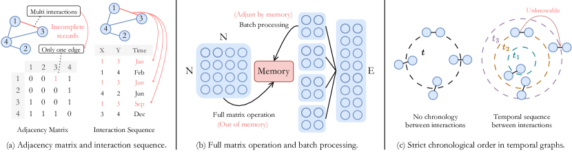
Figure 1: Difference between static graph and temporal graph.

(1) As shown in Fig. 1 (a), if there are several interactions between two nodes, the adjacency matrix can hardly reflect the dynamic structure, especially when these interactions belong to different timestamps. In contrast, temporal graphs utilize the interaction sequence (i.e., adjacency list) to store interactions, thus the above interactions can be clearly and independently recorded. Although some methods also use adjacency list to store edges, the missing record of timestamps can cause multiple interactions at different timestamps to be treated at the same time (Fig. 1 (c)).

(2) Further, we can find in Fig. 1 (b), static graph methods usually train the whole adjacency matrix, which is not convenient enough for large-scale graphs (i.e., possible out-of-memory problem). By slicing the interaction sequence into multiple batches, temporal methods are naturally suitable for large-scale data processing (i.e., batch size can adjust by memory). And it also means that temporal methods can no longer take advantage of the node clustering modules based on the adjacency matrix.

(3) Although there are a few static methods that split graph data into multiple sub-graphs to solve the out-of-memory problems, this still differs from temporal methods. The most important issue is that the loading of temporal graphs must strictly follow the chronological order, i.e., the earlier nodes cannot "see" the later nodes, as shown in Fig. 1 (c). In this case, the temporal relationship of node interactions should still be taken into account during training.

(4) Due to these discrepancies, the difficulty of temporal graph clustering is to find the balance between interaction sequence-based batch-processing patterns and adjacency matrix-based node clustering modules. Nowadays, there is little work to comprehensively discuss it. Although a few methods refer to temporal graph clustering, they are incomplete and will be discussed below.

Driven by this, we propose a simple and scalable framework for Temporal Graph Clustering, called TGC. Such framework adjusts two common deep clustering techniques (i.e., node assignment distribution and graph reconstruction) to suit the batch-processing pattern of temporal graphs. In addition, we discuss temporal graph clustering at several levels, including intuition, complexity, data, and experiment. To verify the superiority of the proposed framework TGC on unsupervised temporal graph representation learning, we conduct extensive experiments. The experimental results show that temporal graph clustering enables more flexibility in finding a balance between time and space requirements, and our framework can effectively improve the performance of existing temporal graph learning methods. In summary, our contributions are several-fold:

Problem. We discuss the differences between temporal graph clustering and static graph clustering. We consider this to be an early work that focuses comprehensively on temporal graph clustering.

Algorithm. We propose a sample general framework TGC, which adds two classical deep clustering techniques to suit the interaction sequence-based batch-processing pattern of temporal graphs.

Dataset. We collated several datasets suitable for temporal graph clustering, and develop two academic citation datasets arXivAI and arXivCS for large-scale temporal graph clustering.

Evaluation. We conduct several experiments to validate the clustering performance, flexibility, and transferability of TGC, and further elucidate the characteristics of temporal graph clustering.

2 Related work

Node clustering is a classic and important unsupervised task in graph learning Hamilton (2020), usually called graph clustering. The utilization of deep learning techniques for graph clustering has become a research trend, and a plethora of methods have surfaced in recent years, such as GraphEncoder Tian et al. (2014), DNGR Cao et al. (2016), DAEGC Wang et al. (2019), MVGRL Hassani and Khasahmadi (2020), AGE Cui et al. (2020), SDCN Bo et al. (2020), DFCN Tu et al. (2021), CGC Park et al. (2022), etc. Most of these methods are based on static graphs that match different modules on the adjacency matrix, the most common being the soft assignment distribution and graph reconstruction. Nevertheless, deep clustering for temporal graphs has not been fully explored. Unlike static graphs, temporal graphs focus more on time information between nodes, which plays an important role in dynamic graphs.

Dynamic graphs can be divided into discrete graphs (discrete-time dynamic graphs, DTDG) and temporal graphs (continuous-time dynamic graphs, CTDG). Discrete graphs generate multiple static snapshots based on the fixed time interval, each snapshot can be seen as a static graph and all snapshots are sorted chronologically Gao and Ribeiro (2021); Wu et al. (2021). In this case, discrete graphs can still be handled with common graph clustering technologies. In contrast, temporal graph learning discards the adjacency matrix and turns to record node interactions based on the sequence directly Trivedi et al. (2019); Liu et al. (2022a). Thus temporal graph methods can divide data into batches and then feed it into the model for one single batch, such as HTNE Zuo et al. (2018), JODIE Kumar et al. (2019), TGAT Xu et al. (2020), TGN Rossi et al. (2020), MNCI Liu and Liu (2021), TREND Wen and Fang (2022), etc.

In fact, most temporal graph methods focus on link prediction rather than node clustering, which we attribute to the facts: On the one hand, temporal graph datasets rarely have corresponding node labels, and their data types are more suitable for targeting edges rather than nodes. On the other hand, the existing clustering techniques need to be adapted for the temporal graphs. Although there are very few methods that refer to the concept of temporal graph clustering from different perspectives, we should still point out that their description of temporal graph clustering is not sufficient:

(1) CGC Park et al. (2022) claims to conduct the experiment of temporal graph clustering, but in fact, the experiment is based on discrete graphs and only carries out on one dataset. We acknowledge that discrete graphs and temporal graphs are inter-convertible, but temporal graphs have a more granular way of observing data than discrete graphs. Moreover, discrete graphs have to be processed as static graphs for each snapshot, which means that it can hardly process large-scale or multi-time graphs. Thus we cannot give up the novel data processing pattern of temporal graph methods, which is one of the implications of temporal graph clustering. As the same reason, RTSC You et al. (2021), VGRGMM Li et al. (2022) and Yao et al. Yao and Joe-Wong (2021) are successful on discrete graphs, but not applicable to temporal graphs. In addition, it is also difficult to find their public datasets and codes for comparison from the web.

(2) GRACE Yang et al. (2017) is a classical graph clustering method. Although its title includes "dynamic embedding", it actually refers to dynamic self-adjustment, which is still a static graph. STAR Xu et al. (2019) and above Yao et al. Yao and Joe-Wong (2021) focus on node classification in temporal graphs, which is a mismatch with the node clustering task. In addition, they provide some potentially usable datasets for temporal graph clustering, which we will discuss in the experimental section.

Through the introduction of some related work (more works will be described in Appendix), we consider that there is little comprehensive discussion of temporal graph clustering. With this motivation, we propose the general framework TGC and further discuss temporal graph clustering.

3 Method

In this section, we first give the definitions of temporal graph clustering, and then describe the proposed framework TGC. Our framework contains two modules: a temporal module for time information mining, and a clustering module for node clustering. Here we introduce the classical HTNE Zuo et al. (2018) method as the baseline of temporal loss, and further discuss the transferability of TGC on other methods in the experiments. For the clustering loss, we improve two classical node clustering methods to fit temporal graphs, i.e., node-level distribution and batch-level reconstruction.

3.1 Problem definition

If a graph contains timestamp records between node interactions, we call it a temporal graph.

Definition 1.

Temporal graph. Given a temporal graph $G=(V,E,T)$, where $V$ denotes nodes and $E$ denotes interactions. In temporal graphs, the concept of edges is replaced by interactions. Because although there is only one edge between two nodes, there may be multiple interactions that occur at different times. Multiple interactions between two nodes can be formulated as: $T_{x,y}=\{(x,y,t_{1}),(x,y,t_{2}),\cdots,(x,y,t_{n})\}$.

If two nodes interact with each other, we call them neighbors. When a node’s neighbors are sorted by interaction time, its historical neighbor sequence is formed.

Definition 2.

Historical neighbor sequence. Given a node $x$, its historical neighbor sequence can be formulated as: $N_{x}=\{(y_{1},t_{1}),(y_{2},t_{2}),\cdots,(y_{l},t_{l})\}$. Such sequence is usually used by temporal graph methods to replace the adjacency matrix as the primary information source.

In the actual training, we use a hyper-parameter $l$ to control the sequence length and preferentially keep neighbors with closer interaction time with $x$. This pattern of controlling length is common in temporal graph learning Zuo et al. (2018); Lu et al. (2019); Xu et al. (2020); Wang et al. (2021); Wen and Fang (2022); Liu et al. (2023), and we discuss it in Appendix.

Finally, temporal graph clustering aims to group nodes into different clusters on temporal graphs.

Definition 3.

Temporal graph clustering. Node clustering in the graph follows some rules: (1) nodes in a cluster are densely connected, and (2) nodes in different clusters are sparsely connected. Here we define $K$ clusters to divide all nodes, i.e., $C=\{c_{1},c_{2},...,c_{K}\}$. Node clustering on the temporal graph usually follows the interactive sequence-based batch-processing pattern to obtain node embeddings, i.e., the clustering centers are continuously updated as more interactions occur. Such node embeddings will be fed into the K-means algorithm for performance evaluation.

3.2 Baseline temporal loss

How to capture the temporal information is the most important problem in temporal graph learning. As a classical temporal graph method, HTNE Zuo et al. (2018) introduces the Hawkes process Hawkes (1971) to capture the dynamic information in graph evolution. Such a process argues that node interactions are influenced by historical interactions and this influence decays over time. Given two nodes $x$ and $y$ interact at time $t$, their conditional interaction intensity $\lambda_{(x,y,t)}$ can be formulated as follows.

$$\lambda_{(x,y,t)}=\mu_{(x,y,t)}+h_{(x,y,t)}$$ (1)

According to Eq. 1, the conditional intensity can be divided into two parts: (1) the base intensity between two nodes without any external influences, i.e., $\mu_{(x,y,t)}=-||\bm{z}_{x}^{t}-\bm{z}_{y}^{t}||^{2}$, where $\bm{z}_{x}^{t}$ is the node embedding of $x$ at time $t$; (2) the hawkes intensity $h_{(x,y,t)}$ from historical interaction influences, which is weighted by node similarity in addition to decaying over time.

$$h_{(x,y,t)}=\sum_{i\in N_{x}}\alpha_{(i,y,t)}\cdot\mu_{(i,y,t)},\quad\alpha_{(i,y,t)}=\omega_{(i,x)}\cdot f(t_{c}-t_{i})$$ (2)

Here, $\omega_{(i,x)}$ is the node similarity weight to evaluate a neighbor’s importance in all neighbors. $f(t_{c}-t_{i})$ denotes the influences from neighbors decay with time, and the earlier the time, the less the influence. $\delta_{t}$ is a learnable parameter, $t_{c}$ denotes the current timestamp.

$$\omega_{(i,x)}=\frac{\exp(\mu_{(i,x)})}{\sum_{i^{\prime}\in N_{x}}\exp(\mu_{(i^{\prime},x)})},\quad f(t_{c}-t_{i})=\exp(-\delta_{t}(t_{c}-t_{i}))$$ (3)

Finally, given two nodes $x$ and $y$ interact at time $t$, their conditional intensity should be as large as possible, and the intensity of node $x$ with any other node should be as small as possible. Since it requires a large amount of computation to calculate the intensities of all nodes, we introduce the negative sampling technology Mikolov et al. (2013), which samples several unrelated nodes as negative samples. Thus the baseline temporal loss function can be calculated as follows, where $P(x)$ is the sampling distribution that is positively correlated with the degree of node $x$.

$$L_{tem}=-\log\sigma(\lambda_{(x,y,t)})-\sum_{n\sim P(x)}\log\sigma(1-\lambda_{(x,n,t)})$$ (4)

For the above temporal information modeling, we introduce a classic HTNE method as the baseline without any additional changes. But the use of time alone is not enough to improve the performance of temporal graph clustering, so we propose clustering loss to compensate for this.

3.3 Improved clustering loss

Compared with static graph clustering, temporal graph clustering faces the challenge that deep clustering modules based on static adjacency matrix are no longer applicable. Since temporal graph methods train data in batches, we need to propose new batch-based modules for node clustering. To restore the classical modules in static graph clustering and ensure their validity, we design two improved modules: node-level distribution and batch-level reconstruction.

3.3.1 Node-level distribution

In this module, we focus on assigning all nodes to different clusters. Especially, for each node $x$ and each cluster $c_{k}$, we utilize the Student’s t-distribution Van der Maaten and Hinton (2008) as the kernel to measure their similarity.

$$q_{(x,k,t)}=\frac{(1+||\bm{z}_{x}^{0}-\bm{z}_{c_{k}}^{t}||^{2}/v)^{-\frac{v+1}{2}}}{\sum_{c_{j}\in C}(1+||\bm{z}_{x}^{0}-\bm{z}_{c_{j}}^{t}||^{2}/v)^{-\frac{v+1}{2}}}$$ (5)

Here $q_{(x,k,t)}$ denotes the probability of assigning node $x$ to cluster $c_{k}$, and $v$ is the degrees of freedom (default value is 1) for Student’s t-distribution Bo et al. (2020). $\bm{z}_{x}^{0}$ denotes the initial feature of node $x$, $\bm{z}_{c_{k}}^{t}$ is one clustering center embedding initialized by K-means on initial node features.

Considering that $q_{(x,k,t)}$ and $\bm{z}_{x}^{0}$ need to be as reliable as possible, and not all temporal graph datasets provide original features to ensure such reliability. Therefore, we select the classical method node2vec to generate initial features for nodes by mining the graph structure, which is equivalent to the pre-training. Note that many graph clustering methods use classical model pre-train to generate initialized clustering centers, such as SDCN Bo et al. (2020) utilizes AE, DFCN Tu et al. (2021) and DCRN Liu et al. (2022b) utilize GAE, etc. Our choice of node2vec is also not deliberate, and other classical methods can be used as well.

After calculating the soft assignment distribution, we aim to optimize the node embeddings by learning from the high-confidence assignments. In particular, we encourage all nodes to get closer to cluster centers, thus the target distribution $p_{(x,k,t)}$ at time $t$ can be calculated as follows.

$$p_{(x,k,t)}=\frac{q^{2}_{(x,k,t)}/\sum_{i\in V}q_{(i,k,t)}}{\sum_{c_{j}\in C}(q^{2}_{(x,j,t)}/\sum_{i\in V}q_{(i,j,t)})}$$ (6)

The target distribution squares and normalizes each node-cluster pair in the assignment distribution to encourage the assignments to have higher confidence, then we can consider it as the "correct" distribution. We introduce the KL divergence Kullback and Leibler (1951) to the node-level distribution loss, where the real-time assignment distribution is aligned with the target distribution.

$$L_{node}=\sum_{c_{k}\in C}p_{(x,k,t)}\log\frac{p_{(x,k,t)}}{q^{\prime}_{(x,k,t)}}$$ (7)

Note that $q^{\prime}_{(x,k,t)}$ is calculated from node embeddings and can change with the update of node embeddings. This loss function aims to encourage the real-time assignment distribution as close as possible to the target distribution, so that the node embeddings can be more suitable for clustering.

The calculation of the assignment distribution differs in the static and temporal graphs. In static graph clustering, all nodes are computed simultaneously for the distribution. However, there is a sequential order of interactions in temporal graphs, so we calculate the distribution of the nodes in each interaction by batches. Note that if a node has multiple interactions, its distribution will be calculated multiple times, which we consider as multiple calibrations for important nodes.

3.3.2 Batch-level reconstruction

As another classical clustering technology, graph reconstruction also plays an important role, which can be considered as the pretext task of node clustering. Due to the batch training of temporal graphs, the adjacency matrix-based reconstruction technology can hardly be applied in the temporal methods, thus we propose the batch-level module to simply simulate the adjacency relationships reconstruction.

As mentioned above, for each batch, we calculate the temporal conditional intensity between node $x$ and $y$. To achieve that, we obtain the historical sequence $N_{x}$ of $x$. It means that both target node $y$ and neighbor nodes $h\in N_{x}$ have edges with $x$ in the graph, i.e., their adjacency relations are all 1. In addition, in the temporal loss function (Eq. 4), we also sample some negative nodes $n\sim P(x)$, which have no edges with $x$ in the real graph, i.e., their adjacency relations are all 0.

Based on the adjacency relationships above, the embedding of these nodes should also follow this constraint. Thus we utilize the cosine similarity to measure the relationship between two node embeddings and constrain them as close to 1 or 0 as possible. The cosine similarity between two node embeddings can be calculated as $\text{cos}(\bm{z}_{x},\bm{z}_{y})=\frac{\bm{z}_{x}\cdot\bm{z}_{y}}{||\bm{z}_{x}||\cdot||\bm{z}_{y}||}$.

This pseudo-reconstruction operation on batches, while not fully restoring the adjacency matrix reconstruction, uses as many nodes as possible that appear in the batch. It is equivalent to a simple reconstruction of the adjacency matrix without increasing the time complexity, which may provide a new idea for the problem that there is no adjacency matrix in batch processing of temporal graphs. Finally, the batch-level loss function can be formulated as follows.

$$L_{batch}=|1-\text{cos}(\bm{z}_{x}^{t},\bm{z}_{y}^{t})|+|1-\text{cos}(\bm{z}_{x}^{t},\bm{z}_{h}^{t})|+|0-\text{cos}(\bm{z}_{x}^{t},\bm{z}_{n}^{t})|$$ (8)

Thus the improved clustering loss function can be formulated as $L_{clu}=L_{node}+L_{batch}$.

3.4 Loss function and complexity analysis

Our total loss function includes temporal loss and clustering loss, which can be formulated as follows.

$$L=\sum_{(x,y,t)}^{E}(L_{tem}+L_{clu})$$ (9)

Note that the temporal graph is trained in batches, and this division of batches is not related to the number of nodes $N$, but to the length of the interaction sequence $|E|$ (i.e., the total number of interactions). This means that the main complexity of the method for temporal graph clustering is $O(|E|)$, rather than $O(N^{2})$ for static graph clustering because the temporal graph method does not need to call the whole adjacency matrix. In other words, compared to static graph clustering, temporal graph clustering has the advantage of being more flexible and convenient for training:

(1) In the vast majority of cases, $|E|$ is smaller than $N^{2}$ because the upper bound of $|E|$ is $N^{2}$ (when the graph is fully connected), which means that $O(|E|)<O(N^{2})$ in most time.

(2) In individual cases, there is a case where $|E|>N^{2}$, which means that there are multiple interactions between a large number of node pairs. This underscores the superiority of dynamic interaction sequences over adjacency matrices, as the latter compresses multiple interactions into a single edge, leading to a significant loss of information.

(3) The above discussion applies not only to the time complexity but also to the space complexity. As the interaction sequence is arranged chronologically, it can be partitioned into multiple batches of varying sizes. The maximum batch size is primarily determined by the available memory of the deployed platform and can be dynamically adjusted to match the memory constraints. Therefore, TGC can be deployed on many platforms without strict memory requirements.

The different types of datasets mentioned above are all considered in our experiments, which have very different node degrees and sizes. Then We conduct experiments and discussions around these datasets from multiple domains.

4 Datasets

A factor limiting the development of temporal graph clustering is that it is difficult to find a dataset suitable for clustering. Although node clustering is an unsupervised task, we need to use node labels when verifying the experimental results. Most public temporal graph datasets suffer from the following problems. (1) Researchers mainly focus on link prediction without node labels. Thus many public datasets have no labels (such as Ubuntu, Math, Email, and Cloud). (2) Some datasets have only two labels (0 and 1), i.e., models on these datasets aim to predict whether a node is active at a certain timestamp. Node classification tasks on these datasets tend to be more binary-classification than multi-classification, thus these datasets are also not suitable for clustering tasks (such as Wiki, CollegeMsg, and Reddit). (3) Some datasets’ labels do not match their own characteristics, e.g., different ratings of products by users can be considered as labels, but it is difficult to say that these labels are more relevant to the product characteristics than the product category labels, thus leading to the poor performance of all methods on these datasets (such as Bitcoin, ML1M, Yelp, and Amazon).

Constrained by these problems, as shown in Table 1, we do our best to select these suitable datasets from 20+ datasets: DBLP Zuo et al. (2018) is an academic co-author graph, Brain Preti et al. (2017) is a human brain tissue connectivity graph, Patent Hall et al. (2001) is a patent citation graph, School Mastrandrea et al. (2015) is a high school student interaction dataset, arXivAI and arXivCS are two public citation graphs.

In Table 1, Nodes denotes the node number, and Interactions denotes the interaction number. Note that we also report Edges, which represents the edge number in the adjacency matrix when we compress temporal graphs into static graphs for traditional graph clustering methods (As mentioned in Fig. 1, some duplicate interactions are missing). Complexity denotes the main complexity comparison between static graph clustering and temporal graph clustering, Timestamps means interaction time, $K$ means the number of clusters (label categories), and Degree means node average degree. MinI and MaxI denote the maximum and minimum interaction times of nodes, respectively.

Note that we specifically develop two large-scale graphs (arXivAI and arXivCS) for large-scale temporal graph clustering, which record the academic citations on the arxiv website . Their original data are from the OGB benchmark Wang et al. (2020), but are not applicable to temporal graph clustering. We extracted reference records from the original data to construct node interactions with timestamps and then find the corresponding node ids to construct the interaction sequence-style temporal graph. To generate node labels suitable for clustering, we select the domain to which the paper belongs as its node label. Specifically, the arXiv website categorizes computer domains into 40 categories. We first identify the domains that correspond to the nodes, and then convert them into node labels.

On the basis of arXivCS, we also construct the arXivAI dataset by extracting Top-5 relevant domains to AI from the original 40 domains and used them as the basis to extract the corresponding nodes and interactions. These Top-5 domains are Artificial Intelligence (arxiv cs ai), Neural and Evolutionary Computing (arxiv cs ne), Computer Vision and Pattern Recognition (arxiv cs cv), Machine Learning (arxiv cs lg), and Computation and Language (arxiv cs cl). The experimental results show that the extracted arXivAI dataset is more suitable for node clustering than the arXivCS dataset.

Table 1: Dataset statistics.

Datasets	Nodes	Interactions	Edges	Complexity	Timestamps	$K$	Degree	MinI	MaxI
DBLP	28,085	236,894	162,441	$N^{2}\gg E$	27	10	16.87	1	955
Brain	5,000	1,955,488	1,751,910	$N^{2}>E$	12	10	782	484	1,456
Patent	12,214	41,916	41,915	$N^{2}\gg E$	891	6	6.86	1	789
School	327	188,508	5,802	$N^{2}<E$	7,375	9	1153	7	4,647
arXivAI	69,854	699,206	699,198	$N^{2}\gg E$	27	5	20.02	1	11,594
arXivCS	169,343	1,166,243	1,166,237	$N^{2}\gg E$	29	40	13.77	1	13,161

5 Experiments

In this part, we discuss the experiment results. Due to the limitation of space, we present some of the descriptions and experiments in the appendix. Here we ask several important questions about the experiment: Q1: What are the advantages of TGC? Q2: Is the memory requirement for TGC really lower? Q3: Is TGC valid for existing temporal graph learning methods? Q4: What restricts the development of temporal graph clustering?

5.1 Baselines

To demonstrate the performance of TGC, we compare it with multiple state-of-the-art methods as baselines. In particular, we divide these methods into three categories: Classic methods refer to some early and highly influential methods, such as DeepWalk Perozzi et al. (2014), AE Hinton and Salakhutdinov (2006), node2vec Grover and Leskovec (2016), GAE Kipf and Welling (2016), etc. Deep graph clustering methods refer to some methods that focus on clustering nodes on static graphs, such as MVGRL Hassani and Khasahmadi (2020), AGE Cui et al. (2020), DAEGC Wang et al. (2019), SDCN (and SDCNQ) Bo et al. (2020), DFCN Tu et al. (2021), etc. Temporal graph learning methods refer to some methods that model temporal graphs without node clustering task, such as HTNE Zuo et al. (2018), TGAT Xu et al. (2020), JODIE Kumar et al. (2019), TGN Rossi et al. (2020), TREND Wen and Fang (2022), etc.

5.2 Node Clustering Performance

Table 2: Node clustering results in common datasets. We bold the best results and underline the second best results. If a method face the out-of-memory problem, we record as OOM.

Data	Metric	deepwalk	AE	node2vec	GAE	MVGRL	AGE	DAEGC	SDCN	SDCNQ	DFCN	HTNE	TGAT	JODIE	TGN	TREND	TGC
DBLP	ACC	28.95	42.16	46.31	39.31	28.95	OOM	OOM	46.69	40.47	41.97	45.74	36.76	20.79	19.78	25.36	48.75
	NMI	22.03	36.71	34.87	29.75	22.03	OOM	OOM	35.07	31.86	36.94	35.95	28.98	11.67	9.82	14.25	37.08
	ARI	13.73	22.54	20.40	17.17	13.73	OOM	OOM	23.74	19.80	21.46	22.13	17.64	11.32	5.46	6.24	22.86
	F1	24.79	37.84	43.35	35.04	24.79	OOM	OOM	40.31	35.18	35.97	43.98	34.22	13.23	10.66	19.89	45.03
Brain	ACC	41.28	43.48	43.92	31.22	15.76	38.48	42.52	42.62	43.42	47.46	43.20	41.43	19.14	17.40	39.83	44.30
	NMI	49.09	50.49	45.96	32.23	21.15	39.64	49.86	46.61	47.40	48.53	50.33	48.72	10.50	8.04	45.64	50.68
	ARI	28.40	29.78	26.08	14.97	9.77	28.82	27.47	27.93	27.69	28.58	29.26	23.64	5.00	4.56	22.82	30.03
	F1	42.54	43.26	46.61	34.11	13.56	36.47	43.24	41.42	37.27	50.45	43.85	41.13	11.12	13.49	33.67	44.42
Patent	ACC	38.69	30.81	40.36	39.65	31.13	43.28	46.64	37.28	32.76	39.23	45.07	38.26	30.82	38.77	38.72	50.36
	NMI	22.71	8.76	24.84	17.73	10.19	20.72	21.28	13.17	9.11	15.42	20.77	19.74	9.55	8.24	14.44	25.04
	ARI	10.32	7.43	18.95	13.61	10.26	19.23	16.74	10.12	7.84	12.24	10.69	13.31	7.46	6.01	13.45	18.81
	F1	31.48	26.65	34.97	30.95	18.06	35.45	32.83	31.38	28.27	30.32	28.85	26.97	20.83	21.40	28.41	38.69
School	ACC	90.60	30.88	91.56	85.62	32.37	84.71	34.25	48.32	33.94	49.85	99.38	80.54	65.64	31.71	94.18	99.69
	NMI	91.72	21.42	92.63	89.41	31.23	81.51	29.53	53.35	25.79	43.37	98.73	73.25	63.82	19.45	89.55	99.36
	ARI	89.66	12.04	90.25	83.09	25.00	70.24	15.38	33.81	15.82	28.31	98.70	80.04	71.94	32.12	87.50	99.33
	F1	92.63	31.00	91.74	82.64	24.41	84.80	31.39	45.62	33.25	47.05	99.34	79.56	68.53	29.50	94.18	99.69

Table 3: Node clustering results in large-scale datasets. We bold the best results and underline the second best results. If a method face the out-of-memory problem, we record as OOM.

Data	Metric	deepwalk	AE	node2vec	GAE	MVGRL	AGE	DAEGC	SDCN	SDCNQ	DFCN	HTNE	TGAT	JODIE	TGN	TREND	TGC
arXivAI	ACC	60.91	23.85	65.01	38.72	OOM	OOM	OOM	44.44	37.62	OOM	65.66	48.69	30.71	31.25	32.79	73.59
	NMI	34.34	10.20	36.18	32.54	OOM	OOM	OOM	21.63	20.73	OOM	39.24	32.12	32.16	24.74	19.82	42.46
	ARI	36.08	14.00	40.35	32.98	OOM	OOM	OOM	23.43	21.29	OOM	43.73	30.34	33.47	11.91	25.37	48.98
	F1	49.47	19.20	53.66	16.97	OOM	OOM	OOM	33.96	31.62	OOM	52.86	43.62	19.91	21.93	23.09	57.86
arXivCS	ACC	29.98	24.20	27.39	OOM	OOM	OOM	OOM	29.78	27.05	OOM	25.57	20.53	11.27	20.10	18.94	39.95
	NMI	40.86	14.03	41.18	OOM	OOM	OOM	OOM	13.27	11.57	OOM	40.83	38.64	15.50	16.21	25.58	43.89
	ARI	15.75	11.80	19.14	OOM	OOM	OOM	OOM	14.32	12.02	OOM	16.51	15.54	25.74	18.63	23.48	36.06
	F1	20.39	12.33	21.41	OOM	OOM	OOM	OOM	14.08	13.28	OOM	19.56	13.23	12.71	22.67	14.55	25.46

Q1: What are the advantages of TGC? Answer: TGC is more adapted to high overlapping graphs and large-scale graphs. As shown in Table 2 and 3, we can observe that:

(1) Although TGC may not perform optimally on all datasets, the aggregate results are leading. Especially on large-scale datasets, many static clustering methods face the out-of-memory (OOM) problem on GPU (we use NVIDIA RTX 3070 Ti), only SDCN benefits from a simpler architecture and can run on the CPU (not GPU). This is due to the overflow of adjacency matrix computation caused by the excessive number of nodes, and of course, the problem can be avoided by cutting subgraphs. Nevertheless, we also wish to point out that by training the graph in batches, temporal graph learning can naturally avoid the OOM problem. This in turn implies that temporal graph clustering is more flexible than static graph clustering on large-scale temporal graph datasets.

(2) The performance varies between different datasets, which we believe is due to the datasets belonging to different fields. For example, the arXivCS dataset has 40 domains and some of which overlap, thus it is difficult to say that each category is distinctly different, so the performance is relatively low. On the contrary, node labels of the School dataset come from the class and gender that students are divided into. Students in the same class or sex often interact more frequently, which enables most methods to distinguish them clearly. Note that on the School dataset, almost all temporal methods achieve better performance than static methods. This echoes the complexity problem we analyzed above, as the only dataset where $N^{2}<E$, the dataset loses the vast majority of edges when we transfer it to the adjacency matrix, thus static methods face a large loss of valid information.

(3) The slightly poor performance of temporal graph learning methods compared to deep graph clustering methods supports our claim that current temporal graph methods do not yet focus deeply on the clustering task. In addition, after considering the clustering task, TGC surpasses the static graph clustering method, also indicating that time information is indeed important and effective in the temporal graph clustering task. Note that these temporal methods achieve different results due to different settings, but we consider our TGC framework can effectively help them improve the clustering performance. Next, we will discuss TGC’s memory usage and transferability.

5.3 GPU memory usage study

Q2: Is the memory requirement for TGC really lower? Answer: Compared to static graph clustering methods, TGC significantly reduces memory requirements.

We first compare the memory usage of static clustering methods and TGC on different datasets, which we sort by the number of nodes. As shown in Fig. 2, we report their max memory usage. As the node number increases, the memory usages of static methods become larger and larger, and eventually out-of-memory problem occurs. At the same time, the memory usage of TGC is also gradually increasing, but the magnitude is small and it is still far from the OOM problem.

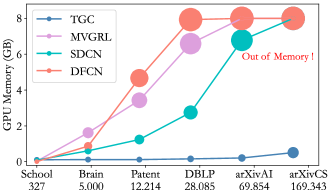
Figure 2: Memory changes between static methods and TGC.

As mentioned above, the main complexity $O(|E|)$ of temporal methods is usually smaller than $O(N^{2})$ of static methods. To name a few, for the arXivCS dataset with a large number of nodes and interactions, the memory usage of TGC is only 212.77 MB, while the memory usage of SDCN, the only one without OOM problem, is 6946.73 MB. For the Brain dataset with a small number of nodes and a large number of interactions, the memory usage of TGC (121.35 MB) is still smaller than SDCN (626.20 MB). We consider that for large-scale temporal graphs, TGC can be less concerned with memory usage, and thus can be deployed more flexibly to different platforms.

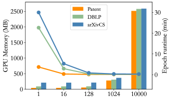
Figure 3: Changes in memory and runtime under different batch sizes.

We further verify that TGC can flexibly adjust the batch size according to the memory. In Fig. 3, we report the memory usages (bar chart) and runtime changes (line chart) under different batch sizes. Generally, the smaller the batch size, the longer the runtime for each epoch. When the batch size is adjusted to 1, the time required for training each epoch comes to a fairly high level. It also reflects the fact that TGC is flexible enough to find a balance between time consumption and space consumption according to actual requirements, either time for space or space for time is feasible.

5.4 Transferability and limitation discussion

Q3: Is TGC valid for existing temporal graph learning methods? Answer: TGC is a simple general framework that can improve the clustering performance of existing temporal graph learning methods.

As shown in Fig. 4, in addition to the baseline HTNE, we also add the TGC framework to TGN and TREND for comparison. Although TGC improves these methods differently, basically they are effective in improving their clustering performance. This means that TGC is a general framework that can be easily applied to different temporal graph methods.

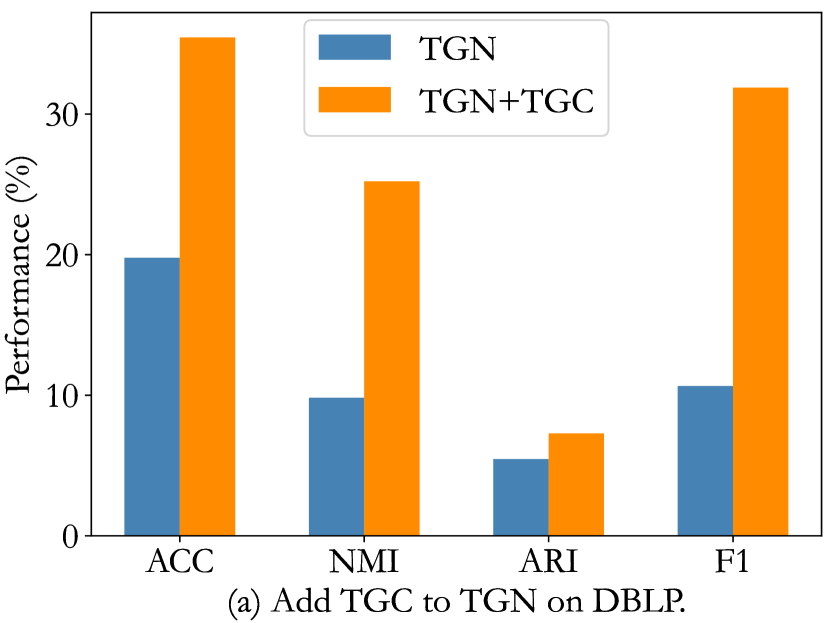
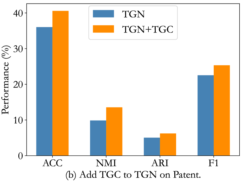
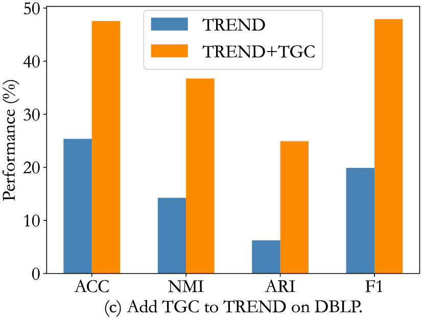
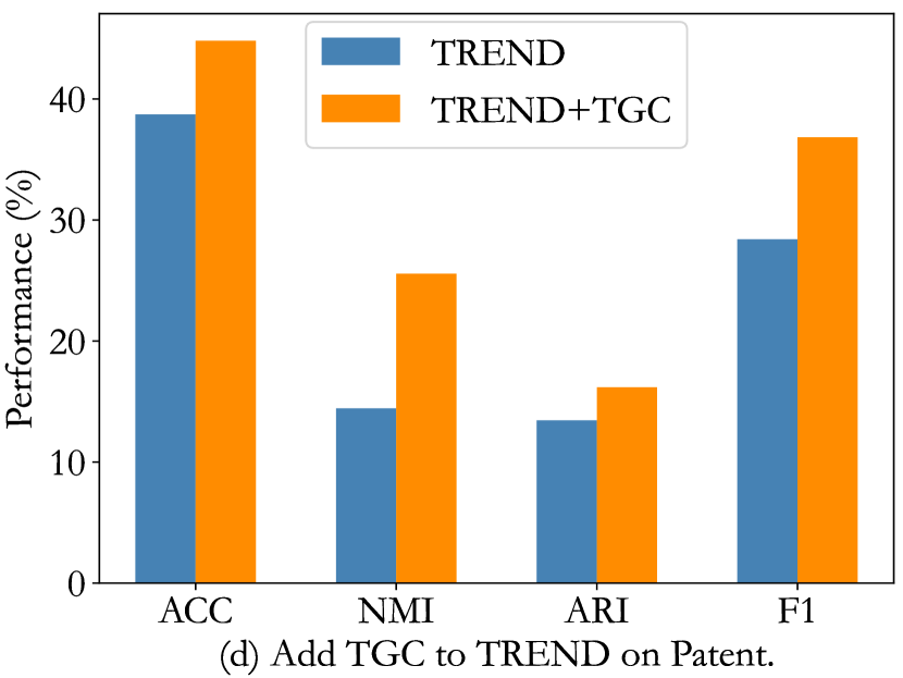
Figure 4: Transferability of TGC on different temporal graph methods.

We also want to ask Q4: What restricts the development of temporal graph clustering? Answer: (1) Few available datasets and (2) information loss without adjacency matrix.

On the one hand, as mentioned above, there are few available public datasets for temporal graph clustering. We collate a lot of raw data and transform them into temporal graphs, and we also discard many of them with low label confidence or incomplete labels. On the other hand, some global information is inevitably lost without adjacency matrix. Since temporal graph clustering is a novel task, there is still a lot of room for expansion of TGC. For example, how to further optimize module migration without adjacency matrix and how to adapt to the incomplete label problem in some graphs.

These issues limit the efficiency and performance of temporal graph clustering, and further exploration is required. In conclusion, although the development of temporal graph clustering is only in its infancy, we cannot ignore its possibility as a new solution.

6 Conclusion

In this paper, we propose a simple general framework TGC for temporal graph clustering. TGC can be extended to existing temporal graph methods, which adapt static graph clustering techniques to the interaction sequence-based batch-processing pattern of temporal graphs. To introduce temporal graph clustering as comprehensively as possible, we discuss the differences between temporal graph clustering and existing static graph clustering at several levels, including intuition, complexity, data, and experiments. Combining experiment results, we demonstrate the effectiveness of our TGC framework on existing temporal graph learning methods and point out that temporal graph clustering enables more flexibility in finding a balance between time and space requirements. In the future, we will further focus on large-scale and $K$-free temporal graph clustering.

References

- Bo et al. [2020] Deyu Bo, Xiao Wang, Chuan Shi, Meiqi Zhu, Emiao Lu, and Peng Cui. Structural deep clustering network. In Proceedings of the web conference 2020, pages 1400–1410, 2020.
- Cao et al. [2016] Shaosheng Cao, Wei Lu, and Qiongkai Xu. Deep neural networks for learning graph representations. In Proceedings of the AAAI conference on artificial intelligence, volume 30, 2016.
- Cui et al. [2020] Ganqu Cui, Jie Zhou, Cheng Yang, and Zhiyuan Liu. Adaptive graph encoder for attributed graph embedding. In Proceedings of the 26th ACM SIGKDD international conference on knowledge discovery & data mining, pages 976–985, 2020.
- Cui et al. [2018] Peng Cui, Xiao Wang, Jian Pei, and Wenwu Zhu. A survey on network embedding. IEEE transactions on knowledge and data engineering, 31(5):833–852, 2018.
- Fan et al. [2022] Wei Fan, Meng Liu, and Yong Liu. A dynamic heterogeneous graph perception network with time-based mini-batch for information diffusion prediction. In Database Systems for Advanced Applications: 27th International Conference, DASFAA 2022, Virtual Event, April 11–14, 2022, Proceedings, Part I, pages 604–612. Springer, 2022.
- Gao and Ribeiro [2021] Jianfei Gao and Bruno Ribeiro. On the equivalence between temporal and static graph representations for observational predictions. arXiv preprint arXiv:2103.07016, 2021.
- Grover and Leskovec [2016] Aditya Grover and Jure Leskovec. node2vec: Scalable feature learning for networks. In Proceedings of the 22nd ACM SIGKDD international conference on Knowledge discovery and data mining, pages 855–864, 2016.
- Hajela et al. [2020] Gaurav Hajela, Meenu Chawla, and Akhtar Rasool. A clustering based hotspot identification approach for crime prediction. Procedia Computer Science, 167:1462–1470, 2020.
- Hall et al. [2001] Bronwyn H Hall, Adam B Jaffe, and Manuel Trajtenberg. The nber patent citation data file: Lessons, insights and methodological tools, 2001.
- Hamilton [2020] William L Hamilton. Graph representation learning. Synthesis Lectures on Artifical Intelligence and Machine Learning, 14(3):1–159, 2020.
- Hassani and Khasahmadi [2020] Kaveh Hassani and Amir Hosein Khasahmadi. Contrastive multi-view representation learning on graphs. In International conference on machine learning, pages 4116–4126. PMLR, 2020.
- Hawkes [1971] Alan G Hawkes. Point spectra of some mutually exciting point processes. Journal of the Royal Statistical Society: Series B (Methodological), 33(3):438–443, 1971.
- Hinton and Salakhutdinov [2006] Geoffrey E Hinton and Ruslan R Salakhutdinov. Reducing the dimensionality of data with neural networks. science, 313(5786):504–507, 2006.
- Kipf and Welling [2016] Thomas N Kipf and Max Welling. Variational graph auto-encoders. In Advances in neural information processing systems, 2016.
- Kullback and Leibler [1951] Solomon Kullback and Richard A Leibler. On information and sufficiency. The annals of mathematical statistics, 22(1):79–86, 1951.
- Kumar et al. [2019] Srijan Kumar, Xikun Zhang, and Jure Leskovec. Predicting dynamic embedding trajectory in temporal interaction networks. In Proceedings of the 25th ACM SIGKDD international conference on knowledge discovery and data mining, pages 1269–1278, 2019.
- Li et al. [2022] Tianpeng Li, Wenjun Wang, Pengfei Jiao, Yinghui Wang, Ruomeng Ding, Huaming Wu, Lin Pan, and Di Jin. Exploring temporal community structure via network embedding. IEEE Transactions on Cybernetics, 2022.
- Liang et al. [2021] Ke Liang, Sifan Wu, and Jiayi Gu. Mka: A scalable medical knowledge-assisted mechanism for generative models on medical conversation tasks. In Computational and Mathematical Methods in Medicine, volume vol. 2021, 2021. doi: 10.1155/2021/5294627.
- Liang et al. [2022a] Ke Liang, Yue Liu, Sihang Zhou, Xinwang Liu, and Wenxuan Tu. Relational symmetry based knowledge graph contrastive learning. arXiv preprint arXiv:2211.10738, 2022a.
- Liang et al. [2022b] Ke Liang, Lingyuan Meng, Meng Liu, Yue Liu, Wenxuan Tu, Siwei Wang, Sihang Zhou, Xinwang Liu, and Fuchun Sun. Reasoning over different types of knowledge graphs: Static, temporal and multi-modal. arXiv preprint arXiv:2212.05767, 2022b.
- Liang et al. [2023] Ke Liang, Jim Tan, Dongrui Zeng, Yongzhe Huang, Xiaolei Huang, and Gang Tan. Abslearn: a gnn-based framework for aliasing and buffer-size information retrieval. Pattern Analysis and Applications, Feb 2023. ISSN 1433-755X. doi: 10.1007/s10044-023-01142-2.
- Liu and Liu [2021] Meng Liu and Yong Liu. Inductive representation learning in temporal networks via mining neighborhood and community influences. In Proceedings of the 44th International ACM SIGIR Conference on Research and Development in Information Retrieval, pages 2202–2206, 2021.
- Liu et al. [2022a] Meng Liu, Jiaming Wu, and Yong Liu. Embedding global and local influences for dynamic graphs. In Proceedings of the 31st ACM International Conference on Information and Knowledge Management, pages 4249–4253, 2022a.
- Liu et al. [2023] Meng Liu, Ke Liang, Bin Xiao, Sihang Zhou, Wenxuan Tu, Yue Liu, Xihong Yang, and Xinwang Liu. Self-supervised temporal graph learning with temporal and structural intensity alignment. arXiv preprint arXiv:2302.07491, 2023.
- Liu et al. [2022b] Yue Liu, Wenxuan Tu, Sihang Zhou, Xinwang Liu, Linxuan Song, Xihong Yang, and En Zhu. Deep graph clustering via dual correlation reduction. In Proceedings of the AAAI Conference on Artificial Intelligence, volume 36, pages 7603–7611, 2022b.
- Lu et al. [2019] Yuanfu Lu, Xiao Wang, Chuan Shi, Philip S Yu, and Yanfang Ye. Temporal network embedding with micro-and macro-dynamics. In Proceedings of the 28th ACM international conference on information and knowledge management, pages 469–478, 2019.
- Ma et al. [2022] Jiachen Ma, Yong Liu, Meng Liu, and Meng Han. Curriculum contrastive learning for fake news detection. In Proceedings of the 31st ACM International Conference on Information & Knowledge Management, pages 4309–4313, 2022.
- Mastrandrea et al. [2015] Rossana Mastrandrea, Julie Fournet, and Alain Barrat. Contact patterns in a high school: a comparison between data collected using wearable sensors, contact diaries and friendship surveys. PloS one, 10(9):e0136497, 2015.
- Meng et al. [2023] Lingyuan Meng, Ke Liang, Bin Xiao, Sihang Zhou, Yue Liu, Meng Liu, Xihong Yang, and Xinwang Liu. Sarf: Aliasing relation assisted self-supervised learning for few-shot relation reasoning. arXiv preprint arXiv:2304.10297, 2023.
- Mikolov et al. [2013] Tomas Mikolov, Ilya Sutskever, Kai Chen, Greg S Corrado, and Jeff Dean. Distributed representations of words and phrases and their compositionality. Advances in neural information processing systems, 26, 2013.
- Park et al. [2022] Namyong Park, Ryan Rossi, Eunyee Koh, Iftikhar Ahamath Burhanuddin, Sungchul Kim, Fan Du, Nesreen Ahmed, and Christos Faloutsos. Cgc: Contrastive graph clustering forcommunity detection and tracking. In Proceedings of the ACM Web Conference 2022, pages 1115–1126, 2022.
- Perozzi et al. [2014] Bryan Perozzi, Rami Al-Rfou, and Steven Skiena. Deepwalk: Online learning of social representations. In Proceedings of the 20th ACM SIGKDD international conference on Knowledge discovery and data mining, pages 701–710, 2014.
- Preti et al. [2017] Maria Giulia Preti, Thomas AW Bolton, and Dimitri Van De Ville. The dynamic functional connectome: State-of-the-art and perspectives. Neuroimage, 160:41–54, 2017.
- Rossetti and Cazabet [2018] Giulio Rossetti and Rémy Cazabet. Community discovery in dynamic networks: a survey. ACM computing surveys (CSUR), 51(2):1–37, 2018.
- Rossi et al. [2020] Emanuele Rossi, Ben Chamberlain, Fabrizio Frasca, Davide Eynard, Federico Monti, and Michael Bronstein. Temporal graph networks for deep learning on dynamic graphs. arXiv preprint arXiv:2006.10637, 2020.
- Thiprungsri and Vasarhelyi [2011] Sutapat Thiprungsri and Miklos A Vasarhelyi. Cluster analysis for anomaly detection in accounting data: An audit approach. International Journal of Digital Accounting Research, 11, 2011.
- Tian et al. [2014] Fei Tian, Bin Gao, Qing Cui, Enhong Chen, and Tie-Yan Liu. Learning deep representations for graph clustering. In Proceedings of the AAAI Conference on Artificial Intelligence, volume 28, 2014.
- Trivedi et al. [2019] Rakshit Trivedi, Mehrdad Farajtabar, Prasenjeet Biswal, and Hongyuan Zha. Dyrep: Learning representations over dynamic graphs. In International conference on learning representations, 2019.
- Tu et al. [2021] Wenxuan Tu, Sihang Zhou, Xinwang Liu, Xifeng Guo, Zhiping Cai, En Zhu, and Jieren Cheng. Deep fusion clustering network. In Proceedings of the AAAI Conference on Artificial Intelligence, volume 35, pages 9978–9987, 2021.
- Van der Maaten and Hinton [2008] Laurens Van der Maaten and Geoffrey Hinton. Visualizing data using t-sne. Journal of machine learning research, 9(11), 2008.
- Wang et al. [2019] C Wang, S Pan, R Hu, G Long, J Jiang, and C Zhang. Attributed graph clustering: A deep attentional embedding approach. In International Joint Conference on Artificial Intelligence. International Joint Conferences on Artificial Intelligence, 2019.
- Wang et al. [2020] Kuansan Wang, Zhihong Shen, Chiyuan Huang, Chieh-Han Wu, Yuxiao Dong, and Anshul Kanakia. Microsoft academic graph: When experts are not enough. Quantitative Science Studies, 1(1):396–413, 2020.
- Wang et al. [2021] Yanbang Wang, Yen-Yu Chang, Yunyu Liu, Jure Leskovec, and Pan Li. Inductive representation learning in temporal networks via causal anonymous walks. arXiv preprint arXiv:2101.05974, 2021.
- Wen and Fang [2022] Zhihao Wen and Yuan Fang. Trend: Temporal event and node dynamics for graph representation learning. In Proceedings of the ACM Web Conference 2022, pages 1159–1169, 2022.
- Wu et al. [2021] Jiaming Wu, Meng Liu, Jiangting Fan, Yong Liu, and Meng Han. Sagedy: A novel sampling and aggregating based representation learning approach for dynamic networks. In ICANN 2021: 30th International Conference on Artificial Neural Networks, pages 3–15. Springer, 2021.
- Xu et al. [2020] Da Xu, Chuanwei Ruan, Evren Korpeoglu, Sushant Kumar, and Kannan Achan. Inductive representation learning on temporal graphs. In ICLR, 2020.
- Xu et al. [2019] Dongkuan Xu, Wei Cheng, Dongsheng Luo, Xiao Liu, and Xiang Zhang. Spatio-temporal attentive rnn for node classification in temporal attributed graphs. In IJCAI, pages 3947–3953, 2019.
- Yang et al. [2017] Carl Yang, Mengxiong Liu, Zongyi Wang, Liyuan Liu, and Jiawei Han. Graph clustering with dynamic embedding. arXiv preprint arXiv:1712.08249, 2017.
- Yao and Joe-Wong [2021] Yuhang Yao and Carlee Joe-Wong. Interpretable clustering on dynamic graphs with recurrent graph neural networks. In Proceedings of the AAAI Conference on Artificial Intelligence, volume 35, pages 4608–4616, 2021.
- You et al. [2021] Jingyi You, Chenlong Hu, Hidetaka Kamigaito, Kotaro Funakoshi, and Manabu Okumura. Robust dynamic clustering for temporal networks. In Proceedings of the 30th ACM International Conference on Information & Knowledge Management, pages 2424–2433, 2021.
- Zuo et al. [2018] Yuan Zuo, Guannan Liu, Hao Lin, Jia Guo, Xiaoqian Hu, and Junjie Wu. Embedding temporal network via neighborhood formation. In Proceedings of the 24th ACM SIGKDD international conference on knowledge discovery & data mining, pages 2857–2866, 2018.