Unique Solutions to Hyperbolic Conservation Laws with a Strictly Convex Entropy

Abstract

Consider a strictly hyperbolic $n\times n$ system of conservation laws, where each characteristic field is either genuinely nonlinear or linearly degenerate. In this standard setting, it is well known that there exists a Lipschitz semigroup of weak solutions, defined on a domain of functions with small total variation. If the system admits a strictly convex entropy, we give a short proof that every entropy weak solution taking values within the domain of the semigroup coincides with a semigroup trajectory. The result shows that the assumptions of “Tame Variation” or “Tame Oscillation”, previously used to achieve uniqueness, can be removed in the presence of a strictly convex entropy.

1 Introduction

We consider the Cauchy problem for a strictly hyperbolic $n\times n$ system of conservation laws in one space dimension:

$$u_{t}+f(u)_{x}~{}=~{}0,$$ (1.1)

$$u(0,x)~{}=~{}\bar{u}(x).$$ (1.2)

As usual, $f:\Omega\to\mathbb{R}^{n}$ is the flux, defined on some open set $\Omega\subset\mathbb{R}^{n}$. We assume that each characteristic family is either genuinely nonlinear or linearly degenerate. In this setting, it is well known that there exists a Lipschitz continuous semigroup $S:{\cal D}\times[0,+\infty[\,\mapsto{\cal D}$ of entropy weak solutions, defined on a domain ${\cal D}\subset{\bf L}^{1}({\mathbb{R}};\,{\mathbb{R}}^{n})$ containing all functions with sufficiently small total variation [8, 10, 11, 16, 20, 23]. The trajectories of this semigroup are the unique limits of front tracking approximations, and also of Glimm approximations [7] and of vanishing viscosity approximations [6]. We recall that the semigroup is globally Lipschitz continuous w.r.t. the ${\bf L}^{1}$ distance. Namely, there exists a constant $L$ such that

$$\bigl{\|}S_{t}\bar{u}-S_{s}\bar{v}\bigr{\|}_{{\bf L}^{1}}~{}\leq~{}L\Big{(}|t-s|+\|\bar{u}-\bar{v}\|_{{\bf L}^{1}}\Big{)}\qquad\hbox{for all}~{}s,t\geq 0,~{}~{}\bar{u},\bar{v}\in{\cal D}.$$ (1.3)

Given any weak solution $u=u(t,x)$ of (1.1)-(1.2), various conditions have been derived in [12, 14, 15] which guarantee the identity

$$u(t)~{}=~{}S_{t}\bar{u}\qquad\hbox{for all}~{}t\geq 0.$$ (1.4)

Since the semigroup $S$ is unique, the identity (1.4) yields the uniqueness of solutions to the Cauchy problem (1.1)-(1.2). In addition to the standard assumptions, earlier results required some additional regularity conditions, such as “Tame Variation” or “Tame Oscillation”, controlling the behavior of the solution near a point where the variation is locally small.

Aim of the present note is to show that, if the $n\times n$ system (1.1) is endowed with a strictly convex entropy $\eta(\cdot)$, then every entropy-weak solution $t\mapsto u(t)$ taking values within the domain ${\cal D}$ of the semigroup satisfies (1.4). In other words, uniqueness is guaranteed without any further regularity assumption.

As in [12, 14, 15], the proof relies on the elementary error estimate

$$\bigl{\|}u(t)-S_{t}\bar{u}\bigr{\|}_{{\bf L}^{1}}~{}\leq~{}L\cdot\int_{0}^{t}\liminf_{h\to 0+}\,{\bigl{\|}u(\tau+h)-S_{h}u(\tau)\bigr{\|}_{{\bf L}^{1}}\over h}\,d\tau\,.$$ (1.5)

Assuming that the system is endowed with a strictly convex entropy, we will prove that the integrand is zero for a.e. time $\tau\geq 0$. Following an argument introduced in [7], this is achieved by two estimates:

• In a neighborhood of a point $(\tau,y)$ where $u(\tau,\cdot)$ has a large jump, the weak solution $u$ is compared with the solution to a Riemann problem.

• In a region where the total variation is small, the weak solution $u$ is compared with the solution to a linear system with constant coefficients.

The main difference is that here we estimate the lim-inf in (1.5) only at times $\tau$ which are Lebesgue points for a countable family of total variation functions $W^{\xi,\zeta}(\cdot)$, defined at (3.5).

To precisely state the result, we begin by collecting the main assumptions.

• (Conservation equations) The function $u=u(t,x)$ is a weak solution of the Cauchy problem (1.1)-(1.2) taking values within the domain of the semigroup.
  More precisely, $u:[0,T]\mapsto{\cal D}$ is continuous w.r.t. the ${\bf L}^{1}$ distance. The identity $u(0,\cdot)=\bar{u}$ holds in ${\bf L}^{1}$, and moreover

  $$\int\!\!\int\big{(}u\varphi_{t}+f(u)\varphi_{x}\big{)}~{}dxdt=0$$ (1.6)

  for every ${\cal C}^{1}$ function $\varphi$ with compact support contained inside the open strip $\,]0,T[\,\times{\mathbb{R}}$.

Regarding the entropy conditions, we assume that the system (1.1) admits a ${\cal C}^{2}$ entropy function $\eta:\Omega\mapsto{\mathbb{R}}$ with entropy flux $q$, so that the equality $\nabla q(\omega)=\nabla\eta(\omega)Df(\omega)$ holds for all $\omega\in\Omega$. We also assume that the entropy $\eta$ satisfies the strict convexity condition

$$\eta(\omega)~{}\geq~{}\eta(\overline{\omega})+\nabla\eta(\overline{\omega})\cdot(\omega-\overline{\omega})+c_{0}|\omega-\overline{\omega}|^{2},$$ (1.7)

for some $c_{0}>0$ and every couple of states $\omega,\;\overline{\omega}\in\Omega$. As usual, we say that a weak solution $u$ is entropy-admissible if it satisfies:

• (Entropy admissibility condition) For every ${\cal C}^{1}$ function $\varphi\geq 0$ with compact support contained inside the open strip $\,]0,T[\,\times{\mathbb{R}}$, one has

  $$\int\!\!\int\big{(}\eta(u)\varphi_{t}+q(u)\varphi_{x}\big{)}~{}dxdt~{}\geq~{}0.$$ (1.8)

Our result can be simply stated as:

Theorem 1.1.

Let (1.1) be a strictly hyperbolic $n\times n$ system, where each characteristic field is either genuinely nonlinear or linearly degenerate, and which admits a strictly convex entropy $\eta(\cdot)$ as in (1.7). Then every entropy-weak solution $u:[0,T]\mapsto{\cal D}$, taking values within the domain of the semigroup, coincides with a semigroup trajectory.

The theorem will be proved in Section 3. We remark that, restricted to a class of $2\times 2$ systems, a more elaborate proof of this result was recently given in [19].

In our view, the main interest in the above uniqueness theorem is that it opens the door to the study of uniform convergence rates for a very wide class of approximation algorithms. This will be better explained in the concluding remarks, in Section 4.

2 Preliminary lemmas

Let $M$ be an upper bound on the total variation of all functions in the domain $\mathcal{D}$ of the semigroup:

$$\mathop{\mathrm{Tot.Var.}}\left\{u;\mathbb{R}\right\}\leq M,\quad\text{ for all }u\in\mathcal{D}.$$ (2.1)

Since by assumption our solution $u(t,\cdot)\in\mathcal{D}$, for sake of definiteness we shall assume that it is right continuous, namely $u(t,x)=\lim_{y\to x+}u(t,y)$. By [20, Theorem 4.3.1], we have the Lipschitz bound

$$\bigl{\|}u(t_{2},\cdot)-u(t_{1},\cdot)\bigr{\|}_{{\bf L}^{1}({\mathbb{R}})}~{}\leq~{}C_{M}\,(t_{2}-t_{1})\qquad\qquad\hbox{for all}~{}0\leq t_{1}\leq t_{2}\,,$$ (2.2)

for some constant $C_{M}>0$ depending only on $M$ and on the flux $f$.

We begin by reviewing the well known fact that the entropy has finite propagation speed.

Lemma 2.1.

Let $u=u(t,x)$ be a function satisfying (A1) and (A2). Then there exists two constants $\widehat{C},\;\hat{\lambda}>0$ such that the following holds. For any constant state $u^{*}\in\Omega$, any $a<b$, and any $0\leq\tau<\tau^{\prime}$ with $2\hat{\lambda}(\tau^{\prime}-\tau)<b-a$, one has

$$\int_{a+\hat{\lambda}\left(\tau^{\prime}-\tau\right)}^{b-\hat{\lambda}\left(\tau^{\prime}-\tau\right)}\left|u(\tau^{\prime},x)-u^{*}\right|^{2}\;dx~{}\leq~{}\widehat{C}\int_{a}^{b}\left|u(\tau,x)-u^{*}\right|^{2}\;dx.$$ (2.3)

Proof. Given the constant state $u^{*}\in\Omega$, for all $\omega\in\Omega$ define the relative entropy $\eta\left(\omega\mid u^{*}\right)$ and the corresponding entropy flux $q\left(\omega\mid u^{*}\right)$ as

$$\begin{array}[]{rl}\eta\left(\omega\mid u^{*}\right)&=~{}\eta\left(\omega\right)-\eta\left(u^{*}\right)-\nabla\eta\left(u^{*}\right)\left(\omega-u^{*}\right),\\[5.69054pt] q\left(\omega\mid u^{*}\right)&=~{}q\left(\omega\right)-q\left(u^{*}\right)-\nabla\eta\left(u^{*}\right)\bigl{(}f\left(\omega\right)-f\left(u^{*}\right)\bigr{)}.\end{array}$$ (2.4)

The equations (1.6) and (1.8) yield

$$\eta\left(u\mid u^{*}\right)_{t}+q\left(u\mid u^{*}\right)_{x}~{}\leq~{}0,$$ (2.5)

while (1.7) implies

$$\eta\left(\omega\mid u^{*}\right)~{}\geq~{}c_{0}\left|\omega-u^{*}\right|^{2},\qquad\text{ for all }~{}\omega,u^{*}\in\Omega.$$ (2.6)

By the ${\cal C}^{2}$ regularity of the functions $\eta,q$, there exists a constant $C^{\prime}$ such that

$$\eta\left(\omega\mid u^{*}\right)~{}\leq~{}C^{\prime}\left|\omega-u^{*}\right|^{2},\qquad q\left(\omega\mid u^{*}\right)~{}\leq~{}C^{\prime}\left|\omega-u^{*}\right|^{2},\quad\text{ for all }~{}\omega,u^{*}\in\Omega.$$ (2.7)

In view of (2.6), there exists a sufficiently large constant $\hat{\lambda}>0$ such that

$$-\hat{\lambda}\eta\left(\omega\mid u^{*}\right)\pm q\left(\omega\mid u^{*}\right)~{}\leq~{}0,\qquad\text{ for all }~{}\omega,u^{*}\in\Omega.$$ (2.8)

Using (2.5), in connection with test functions that approximate the characteristic function of the trapezoid

$$\Gamma~{}=~{}\bigl{\{}(t,x)\,;~{}\tau<t<\tau^{\prime},~{}~{}a+\hat{\lambda}(t-\tau)<x<b-\hat{\lambda}(t-\tau)\bigr{\}},$$

and recalling (2.8), we obtain

$$\begin{split}\int_{a+\hat{\lambda}(\tau^{\prime}-\tau)}^{b-\hat{\lambda}(\tau^{\prime}-\tau)}\eta\left(u\mid u^{*}\right)\left(\tau^{\prime},x\right)\;dx&~{}\leq~{}\int_{a}^{b}\eta\left(u\mid u^{*}\right)\left(\tau,x\right)\;dx\\ ~{}&\quad+\int_{\tau}^{\tau^{\prime}}\left(-\hat{\lambda}\eta\left(u\mid u^{*}\right)+q\left(u\mid u^{*}\right)\right)\left(t,a+\hat{\lambda}\left(t-\tau\right)\right)\;dt\\ &\quad+\int_{\tau}^{\tau^{\prime}}\left(-\hat{\lambda}\eta\left(u\mid u^{*}\right)-q\left(u\mid u^{*}\right)\right)\left(t,b-\hat{\lambda}\left(t-\tau\right)\right)\;dt\\ &~{}\leq~{}\int_{a}^{b}\eta\left(u\mid u^{*}\right)\left(\tau,x\right)\;dx.\end{split}$$

Together with (2.6)-(2.7), this proves the lemma. MM     

Throughout the following, without loss of generality we shall always assume $\hat{\lambda}=1$. We observe that this can always be achieved by a suitable rescaling of the time variable:

$$\tilde{t}~{}=~{}\kappa t.$$

Similarly, to simplify notation, we also assume that all wave speeds lie in the interval $[-1,1]$.

Given any $\tau\geq 0$ and any bounded interval $]a,b[$ with $-\infty\leq a<b\leq+\infty$, we consider the open intervals

$$J(t)~{}=~{}\bigl{]}a+{}(t-\tau)\,,~{}b-{}(t-\tau)\bigr{[}\,,\qquad\qquad\tau\leq t<\tau+\frac{b-a}{2}\,.$$ (2.9)

Toward the proof of Theorem 1.1, in order to replace the “Tame Variation” condition, the main tool is provided by the following elementary lemma.

Lemma 2.2.

In the setting of Theorem 1.1, for some constant $C>0$ the following holds. Let $u=u(t,x)$ be any entropy weak solution to (1.1). Then

$$\int_{J(t)}\bigl{|}u(t,x)-u(\tau,x)\bigr{|}\,dx~{}\leq~{}C(t-\tau)\cdot\mathop{\mathrm{Tot.Var.}}\bigl{\{}u(\tau,\cdot)\,;~{}]a,b[\bigr{\}}.$$ (2.10)

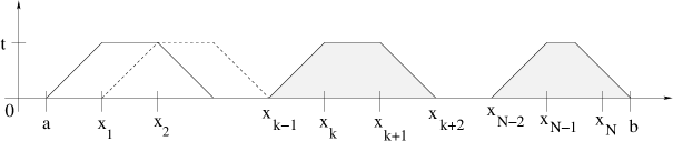
Figure 1: The covering of the interval $[a,b]$ used in the proof of Lemma 2.2.

Proof. 1. We first consider the case where $-\infty<a<b<+\infty$. For notational simplicity, w.l.o.g. we assume that $\tau=0$. Given a time $0<t<\frac{b-a}{2}$, as shown in Fig. 1 we define the points $x_{k}$, the values $u_{k}$ and the integer $N\geq 1$ such that

$$x_{k}~{}=~{}a+kt,\qquad\qquad u_{k}=u(0,x_{k}),\qquad\qquad x_{N}\leq b<x_{N+1}\,.$$ (2.11)

For $k=1,2,\ldots,N-2$, we apply Lemma 2.1 with $u^{*}=u_{k}$ on the trapezoids

$$\Gamma_{k}~{}\doteq~{}\bigl{\{}(s,x)\,;~{}~{}s\in[0,t]\,,~{}~{}x_{k-1}+s<x<x_{k+2}-s\bigr{\}}.$$

Then we apply the same lemma with $u^{*}=u_{N-1}$ on the domain

$$\widetilde{\Gamma}_{N}~{}\doteq~{}\bigl{\{}(s,x)\,;~{}~{}s\in[0,t]\,,~{}~{}x_{N-2}+t<x<b-t\bigr{\}}.$$

This yields the estimates

$$\begin{array}[]{rl}\displaystyle\int_{x_{k}}^{x_{k+1}}\bigl{|}u(t,x)-u_{k}\bigr{|}^{2}\,dx{}&\leq\displaystyle~{}\widehat{C}\,\int_{x_{k-1}}^{x_{k+2}}\bigl{|}u(0,x)-u_{k}\bigr{|}^{2}\,dx\\[11.38109pt] &\leq~{}\widehat{C}\cdot 3t\cdot\Big{(}\mathop{\mathrm{Tot.Var.}}\{u(0,\cdot)\,;~{}]x_{k-1},x_{k+2}[\bigr{\}}\Big{)}^{2},\end{array}$$ (2.12)

$$\int_{x_{N-1}}^{b-t}\bigl{|}u(t,x)-u_{N-1}\bigr{|}^{2}\,dx~{}\leq\displaystyle~{}\widehat{C}\cdot 3t\cdot\Big{(}\mathop{\mathrm{Tot.Var.}}\{u(0,\cdot)\,;~{}]x_{N-2},b[\bigr{\}}\Big{)}^{2}.$$ (2.13)

2. Define the piecewise constant approximation $\bar{u}:[a+t,b-t[\,\mapsto\Omega$ by setting

$$\bar{u}(x)\,=\,u_{k}\qquad\text{ if }~{}x\in\bigl{[}x_{k},x_{k+1}\bigr{[}\,,\qquad\qquad k=1,\ldots,N-1.$$ (2.14)

Using Cauchy’s inequality and the bounds (2.12)-(2.13), we obtain

$$\begin{array}[]{l}\displaystyle\int_{a+t}^{b-t}\bigl{|}u(t,x)-\bar{u}(x)\bigl{|}\,dx~{}=~{}\sum_{k=1}^{N-2}\int_{x_{k}}^{x_{k+1}}\bigl{|}u(t,x)-u_{k}\bigr{|}\,dx+\int_{x_{N-1}}^{b-t}\bigl{|}u(t,x)-u_{N-1}\bigr{|}\,dx\\[11.38109pt] \qquad\displaystyle\leq~{}\sum_{k=1}^{N-2}\sqrt{t}\left(\int_{x_{k}}^{x_{k+1}}\bigl{|}u(t,x)-u_{k-1}\bigr{|}^{2}\,dx\right)^{1/2}+\sqrt{t}\left(\int_{x_{N-1}}^{b-t}\bigl{|}u(t,x)-u_{N-1}\bigr{|}^{2}\,dx\right)^{1/2}\\[11.38109pt] \qquad\displaystyle\leq~{}\sqrt{t}\cdot\sqrt{\widehat{C}\cdot 3t}\cdot\left(\sum_{k=1}^{N-2}\mathop{\mathrm{Tot.Var.}}\{u(0,\cdot)\,;~{}]x_{k-1},x_{k+2}[\bigr{\}}+\mathop{\mathrm{Tot.Var.}}\{u(0,\cdot)\,;~{}]x_{N-2},b[\bigr{\}}\right).\end{array}$$ (2.15)

Observing that every point $x\in[a,b]$ is contained in at most three open intervals $]x_{k-1},x_{k+2}[\,$, from (2.15) we conclude

$$\int_{a+t}^{b-t}\bigl{|}u(t,x)-\bar{u}(x)\bigl{|}\,dx~{}\leq~{}\sqrt{3\widehat{C}}\cdot 3t\cdot\mathop{\mathrm{Tot.Var.}}\bigl{\{}u(0,\cdot)\,;~{}]a,b[\bigr{\}}.$$ (2.16)

3. Next, we compute

$$\begin{array}[]{l}\displaystyle\int_{a+t}^{b-t}\bigl{|}u(0,x)-\bar{u}(x)\bigl{|}\,dx~{}=\displaystyle~{}\sum_{k=1}^{N-2}\int_{x_{k}}^{x_{k+1}}\bigl{|}u(0,x)-u_{k}\bigr{|}\,dx+\int_{x_{N-1}}^{b-t}\bigl{|}u(0,x)-u_{N-1}\bigr{|}\,dx\\[11.38109pt] \quad\leq\displaystyle~{}\sum_{k=1}^{N-2}t\cdot\mathop{\mathrm{Tot.Var.}}\bigl{\{}u(0,\cdot)\,;~{}]x_{k},x_{k+1}[\,\bigr{\}}+t\cdot\mathop{\mathrm{Tot.Var.}}\bigl{\{}u(0,\cdot)\,;~{}]x_{N-1},b-t[\,\bigr{\}}\\[11.38109pt] \quad\displaystyle\leq~{}t\cdot\mathop{\mathrm{Tot.Var.}}\bigl{\{}u(0,\cdot)\,;~{}]a,b[\bigr{\}}.\end{array}$$ (2.17)

Combining (2.16) with (2.17) we obtain a proof of the lemma for finite $a$ and $b$.

Letting $a\to-\infty$ or $b\to+\infty$ we see that the same conclusion remains valid also for unbounded intervals, such as $]-\infty,b[\,$ or $\,]a,+\infty[\,$. MM     

3 Proof of the theorem

We are now ready to give a proof of Theorem 1.1, in several steps. 1. By the structure theorem for BV functions [1, 22], there is a null set of times ${\cal N}\subset[0,T]$ such that the following holds.

Every point $(\tau,\xi)\in[0,T]\times{\mathbb{R}}$ with $\tau\notin{\cal N}$ is either a point of approximate continuity, or a point of approximate jump of the function $u$. In this second case, there exists states $u^{-},u^{+}\in{\mathbb{R}}^{n}$ and a speed $\lambda\in{\mathbb{R}}$ such that, calling

$$U(t,x)~{}\doteq~{}\left\{\begin{array}[]{rl}u^{-}&\hbox{if}\qquad\left(x-\xi\right)<\lambda\left(t-\tau\right),\\[5.69054pt] u^{+}&\hbox{if}\qquad\left(x-\xi\right)>\lambda\left(t-\tau\right),\end{array}\right.$$ (3.1)

there holds

$$\lim_{r\to 0+}~{}{1\over r^{2}}\int_{-r}^{r}\int_{-r}^{r}\Big{|}u(\tau+t,~{}\xi+x)-U(\tau+t,\xi+x)\Big{|}~{}dxdt~{}=~{}0.$$ (3.2)

The conservation equations (1.6) imply that the piecewise constant function $U$ must be a weak solution to the system of conservation laws (see [8, Theorem 4.1]), satisfying the Rankine-Hugoniot equations:

$$f(u^{+})-f(u^{-})~{}=~{}\lambda(u^{+}-u^{-}).$$ (3.3)

Moreover, the entropy condition (1.8) implies

$$q(u^{+})-q(u^{-})~{}\leq~{}\lambda\bigl{(}\eta(u^{+})-\eta(u^{-})\bigr{)}.$$ (3.4)

Next, we observe that, for every couple of rational points $\xi,\zeta\in{\mathbb{Q}}$, the scalar function

$$W^{\xi,\zeta}(t)~{}\doteq~{}\left\{\begin{array}[]{cl}\mathop{\mathrm{Tot.Var.}}\big{\{}u(t)\,;~{}]\xi+t\,,~{}\zeta-t[\,\bigr{\}}&\hbox{if}\quad\xi+t<\zeta-t\,,\\[5.69054pt] 0&\hbox{otherwise,}\end{array}\right.$$ (3.5)

is bounded and measurable (indeed, it is lower semicontinuous). Therefore a.e. $t\in[0,T]$ is a Lebesgue point. We denote by ${\cal N}^{\prime}\subset[0,T]$ the set of all times $t$ which are NOT Lebesgue for at least one of the countably many functions $W^{\xi,\zeta}$. Of course, ${\cal N}^{\prime}$ has zero Lebesgue measure.

In view of (1.5), we will prove the theorem by establishing the following claim.

• For every $\tau\in[0,T]\setminus({\cal N\cup\cal N^{\prime}})$ and $\varepsilon>0$, one has

  $$\limsup_{h\to 0+}{1\over h}\Big{\|}u(\tau+h)-S_{h}u(\tau)\Big{\|}_{{\bf L}^{1}}~{}\leq~{}\varepsilon.$$ (3.6)

2. Assume $\tau\notin\cal N\cup\cal N^{\prime}$. Since $u(\tau,\cdot)$ has bounded variation, we define points

$$-\infty=y_{-1}<y_{0}<y_{1}<\cdots<y_{N}<y_{N+1}=+\infty,$$

$$y_{k+1}~{}=~{}\sup~{}\Big{\{}x>y_{k}\,;~{}~{}\mathop{\mathrm{Tot.Var.}}\bigl{\{}u(\tau,\cdot)\,;~{}~{}]y_{k},x[\,\bigr{\}}\leq\varepsilon\Big{\}}.$$

Since $u(\tau,\cdot)$ is right continuous, we have

$$\begin{cases}\mathop{\mathrm{Tot.Var.}}\bigl{\{}u(\tau,\cdot)\,;~{}]y_{k-1},y_{k}[\,\bigr{\}}~{}\leq~{}\varepsilon,&\text{ for }k=0,\ldots,N+1,\\ \mathop{\mathrm{Tot.Var.}}\bigl{\{}u(\tau,\cdot)\,;~{}]y_{k-1},y_{k}]\,\bigr{\}}~{}\geq~{}\varepsilon,&\text{ for }k=0,\ldots,N,\\ N~{}\leq~{}{M\over\varepsilon}.\end{cases}$$ (3.7)

Where $M$ is an upper bound for the total variation of all functions $\bar{u}\in{\cal D}$, as in (2.1).

Then we choose points $y_{k}^{\prime},y_{k}^{\prime\prime}$ such that

$$-\infty<y_{0}<y_{0}^{\prime\prime}~{}\leq~{}y_{1}^{\prime}<y_{1}<y_{1}^{\prime\prime}~{}\leq~{}y_{2}^{\prime}<y_{2}<y_{2}^{\prime\prime}~{}<~{}\cdots~{}\leq~{}y_{N}^{\prime}<y_{N}<+\infty$$

$$\left\{\begin{array}[]{l}\mathop{\mathrm{Tot.Var.}}\bigl{\{}u(\tau,\cdot)\,;~{}]y^{\prime}_{k},y_{k}[\,\bigr{\}}\,\leq\,\varepsilon^{2},\quad k=1,\ldots N,\\[8.53581pt] \mathop{\mathrm{Tot.Var.}}\bigl{\{}u(\tau,\cdot)\,;~{}]y_{k},y^{\prime\prime}_{k}[\,\bigr{\}}\leq\,\varepsilon^{2},\,\quad k=0,\ldots N-1,\\[8.53581pt] \text{ all values $y_{k}^{\prime}-\tau$, $y^{\prime\prime}_{k}-\tau$ are rational}.\end{array}\right.$$ (3.8)

Figure 2: The points $y^{\prime}_{k}<y_{k}<y^{\prime\prime}_{k}$ constructed in the proof of the theorem. Typically, $y_{k}$ is the location of a shock. Since $y_{k}\pm\tau$ need not be rational, the additional points $y_{k}^{\prime},y_{k}^{\prime\prime}$ must be considered.

3. For any given $y\in{\mathbb{R}}$, we denote by $U^{\sharp}=U^{\sharp}_{(u,\tau,y)}(t,x)$ the solution, for $t\geq\tau$, to the Riemann problem for (1.1) with initial data at $t=\tau$:

$$\bar{u}(x)~{}=~{}\left\{\begin{array}[]{rl}u(\tau,y-)&\hbox{if}~{}~{}x<y,\cr u(\tau,y+)&\hbox{if}~{}~{}x>y.\end{array}\right.$$ (3.9)

Moreover, for every given $k=1,\ldots,N$ we denote by $U^{\flat}=U^{\flat}_{(u,\tau,k)}(t,x)$ the solution to the linear Cauchy problem with constant coefficients

$$v_{t}+Av_{x}~{}=~{}0,\qquad\qquad v(\tau,x)=u(\tau,x).$$ (3.10)

Here the $n\times n$ matrix $A$ is the Jacobian matrix of $f$ computed at the midpoint of the interval $[y^{\prime\prime}_{k-1},y^{\prime}_{k}]$. Namely,

$$~{}A~{}=~{}Df\left(\widetilde{u}_{k}\right),\qquad\widetilde{u}_{k}=u\left(\tau,{y^{\prime\prime}_{k-1}+y^{\prime}_{k}\over 2}\right),\quad k=1,\ldots,N.$$

With reference to Fig. 2, to estimate the lim-sup in (3.6), we need to estimate three types of integrals.

• The integral of $\bigl{|}u(t,x)-U^{\sharp}_{\left(u;\tau,y\right)}(t,x)\bigr{|}$ over the interval

  $$J_{y}(t)~{}\doteq~{}\bigl{[}y-(t-\tau)\,,~{}y+(t-\tau)\bigr{]},$$

  for all points $y\in\bigl{\{}y_{0},y_{0}^{\prime\prime},y_{1}^{\prime},y_{1},y_{1}^{\prime\prime},\ldots,y_{N}^{\prime},y_{N}\bigr{\}}$.

• The integral of $\bigl{|}u(t,x)-U^{\flat}_{\left(u;\tau,k\right)}(t,x)\bigr{|}$ over the interval

  $$J_{k}(t)~{}=~{}\bigl{]}y_{k-1}^{\prime\prime}+(t-\tau)\,,~{}y_{k}^{\prime}-(t-\tau)\bigr{[},\quad k=1,\ldots,N.$$ (3.11)

• The integral of $\bigl{|}u(t,x)-u(\tau,x)\bigr{|}$ over the intervals

  $$\left\{\begin{array}[]{rl}J_{k}^{\prime}(t)&=~{}\bigl{]}y_{k}^{\prime}+(t-\tau)\,,~{}y_{k}-(t-\tau)\bigr{[},\quad k=1,\ldots,N,\\[5.69054pt] J^{\prime\prime}_{k}(t)&=~{}\bigl{]}y_{k}+(t-\tau)\,,~{}y^{\prime\prime}_{k}-(t-\tau)\bigr{[},\quad k=0,\ldots,N-1,\\[5.69054pt] J_{0}(t)&\dot{=}~{}\left]-\infty,y_{0}-\left(t-\tau\right)\right[,\\[5.69054pt] J_{N+1}&\dot{=}~{}\left]y_{N}+\left(t-\tau\right),+\infty\right[.\end{array}\right.$$

4. To estimate integrals of type (I), assuming that $(\tau,y)$ is either a Lebesgue point or a point of approximate jump of the function $u$, we obtain

$$\lim_{h\to 0+}{1\over h}\int_{y-h}^{y+h}\Big{|}u(\tau+h,~{}x)-U^{\sharp}_{(u;\tau,y)}(\tau+h,x)\Big{|}~{}dx~{}=~{}0.$$ (3.12)

Indeed, by [8, Theorem 2.6], setting $u^{\pm}=u\left(\tau,y\pm\right)$, the function $U$ defined in (3.1) satisfies (3.2) and consequently $u^{\pm}$ satisfy (3.3) and (3.4). It implies that $u\left(\tau,y\pm\right)$ are connected by a single entropic shock whose speed is $\lambda$. Consequently $U^{\sharp}_{\left(u;\tau,y\right)}$ coincides with the piecewise constant function $U$ defined in (3.1) so that (3.12) follows from [8, Theorem 2.6].

5. We now estimate the integrals of type (II). By construction, both values $y_{k-1}^{\prime\prime}-\tau$ and $y^{\prime}_{k}+\tau$ are rational. Hence

$$y_{k-1}^{\prime\prime}\,=\,\xi+\tau,\qquad\qquad y_{k}^{\prime}\,=\,\zeta-\tau,$$

for some $\xi,\zeta\in{\mathbb{Q}}$. This implies that $\tau$ is a Lebesgue point of the map

$$t~{}\mapsto~{}V(t)~{}=~{}W^{\xi,\zeta}(t).$$ (3.13)

Let $\tilde{\lambda}_{i}=\lambda_{i}\left(\tilde{u}_{k}\right)$, $\tilde{l}_{i}=l_{i}\left(\tilde{u}_{k}\right)$, $\tilde{r}_{i}=r_{i}\left(\tilde{u}_{k}\right)$, $i=1,\ldots,n$, be respectively the $i$-th eigenvalues and left and right eigenvectors of the matrix $A\doteq Df\big{(}\widetilde{u}_{k}\big{)}$. We thus have

$$\tilde{l}_{i}\cdot U^{\flat}(t,x)~{}=~{}\tilde{l}_{i}\cdot U^{\flat}\big{(}\tau,x-(t-\tau)\tilde{\lambda}_{i}\big{)}~{}=~{}\tilde{l}_{i}\cdot u\big{(}\tau,x-(t-\tau)\tilde{\lambda}_{i}\big{)}.$$

Following the proof of [8, Theorem 9.4], fix any two points $\zeta^{\prime},\zeta^{\prime\prime}\in J_{k}(t)$, $\zeta^{\prime}<\zeta^{\prime\prime}$ and consider the quantity

$$\begin{array}[]{rl}E_{i}(\zeta^{\prime},\zeta^{\prime\prime})&\displaystyle\doteq~{}\tilde{l}_{i}\cdot\int_{\zeta^{\prime}}^{\zeta^{\prime\prime}}\big{(}u(t,x)-U^{\flat}(t,x)\big{)}~{}dx\\[8.53581pt] &=~{}\displaystyle\tilde{l}_{i}\cdot\int_{\zeta^{\prime}}^{\zeta^{\prime\prime}}\Big{(}u(t,x)-u\big{(}\tau,~{}x-(t-\tau)\tilde{\lambda}_{i}\big{)}\Big{)}~{}dx.\end{array}$$ (3.14)

Figure 3: The domain $D_{i}$ considered at (3.15).

We apply the divergence theorem to the vector $\big{(}u,\,f(u)\big{)}$ on the domain

$$D_{i}~{}\doteq~{}\Big{\{}(s,x);~{}~{}s\in[\tau,~{}t],~{}~{}\zeta^{\prime}-(t-s)\tilde{\lambda}_{i}\leq x\leq\zeta^{\prime\prime}-(t-s)\tilde{\lambda}_{i}\Big{\}},$$ (3.15)

shown in Fig. 3. Since $u$ satisfies the conservation equation (1.1), the difference between the integral of $u$ at the top and at the bottom of the domain $D_{i}$ is thus measured by the inflow from the left side minus the outflow from the right side of $D_{i}$. From (3.14) it thus follows

$$\begin{array}[]{rl}E_{i}(\zeta^{\prime},\zeta^{\prime\prime})=&~{}\displaystyle\int_{\tau}^{t}\tilde{l}_{i}\cdot\Big{(}\big{(}f(u)-\tilde{\lambda}_{i}u\big{)}(s,~{}\zeta^{\prime}-(t-s)\tilde{\lambda}_{i})\Big{)}\,ds\cr&\displaystyle\qquad-\int_{\tau}^{t}\tilde{l}_{i}\cdot\Big{(}\big{(}f(u)-\tilde{\lambda}_{i}u\big{)}(s,~{}\zeta^{\prime\prime}-(t-s)\tilde{\lambda}_{i})\Big{)}\,ds\cr=&\displaystyle\int_{\tau}^{t}l_{i}(\tilde{u}_{k})\cdot\Big{(}\big{(}f(u^{\prime}(s))-\tilde{\lambda}_{i}\left(\tilde{u}_{k}\right)u^{\prime}(s)\big{)}-\big{(}f(u^{\prime\prime}(s))-\lambda_{i}(\tilde{u}_{k})u^{\prime\prime}(s)\big{)}\Big{)}\,ds\cr=&\displaystyle\int_{\tau}^{t}H\left(\widetilde{u}_{k},u^{\prime}(s),u^{\prime\prime}(s)\right)\,ds,\end{array}$$ (3.16)

where we set

$$u^{\prime}(s)\doteq u\big{(}s,~{}\zeta^{\prime}-(t-s)\tilde{\lambda}_{i}\big{)},\qquad u^{\prime\prime}(s)\doteq u\big{(}s,~{}\zeta^{\prime\prime}-(t-s)\tilde{\lambda}_{i}\big{)},$$

$$H\left(u,u_{1},u_{2}\right)\,\doteq\,l_{i}(u)\cdot\Big{(}\big{(}f(u_{1})-\lambda_{i}(u)u_{1}\big{)}-\big{(}f(u_{2})-\lambda_{i}(u)u_{2}\big{)}\Big{)}.$$

Observing that

• $H\left(u,u_{2},u_{2}\right)=0$,

• $D_{u_{1}}H\left(u,u_{1},u_{2}\right)=l_{i}(u)\cdot\left(Df(u_{1})-\lambda_{i}(u)I\right)$,

• $D_{u_{1}}H\left(u,u,u_{2}\right)=l_{i}(u)\cdot\left(Df(u)-\lambda_{i}(u)I\right)=0$,

we estimate

$$\begin{array}[]{rl}H\left(u,u_{1},u_{2}\right)&=~{}H\left(u,u_{1},u_{2}\right)-H\left(u,u_{2},u_{2}\right)\\[11.38109pt] &=~{}\displaystyle\int_{0}^{1}D_{u_{1}}H\left(u,u_{2}+\sigma\left(u_{1}-u_{2}\right),u_{2}\right)\;d\sigma\cdot\left(u_{1}-u_{2}\right)\\[11.38109pt] &=~{}\displaystyle\int_{0}^{1}\left[D_{u_{1}}H\left(u,u_{2}+\sigma\left(u_{1}-u_{2}\right),u_{2}\right)-D_{u_{1}}H\left(u,u,u_{2}\right)\right]\;d\sigma\cdot\left(u_{1}-u_{2}\right)\\[11.38109pt] &=~{}\displaystyle{\cal O}(1)\cdot\bigl{(}\left|u_{1}-u\right|+\left|u_{2}-u\right|\bigr{)}\cdot\left|u_{1}-u_{2}\right|.\end{array}$$

Therefore,

$$E_{i}(\zeta^{\prime},\zeta^{\prime\prime})~{}=~{}{\cal O}(1)\cdot\int_{\tau}^{t}\left|u^{\prime}(s)-u^{\prime\prime}(s)\right|\cdot\Big{(}\left|u^{\prime}(s)-\widetilde{u}_{k}\right|+\left|u^{\prime\prime}(s)-\widetilde{u}_{k}\right|\Big{)}\,ds.$$

Recalling (3.11) and (3.13), for any $x\in J_{k}(s)$ we now compute

$$\left|u^{\prime}(s)-\widetilde{u}_{k}\right|\leq V(s)+\left|u\big{(}s,x\big{)}-u\left(\tau,x\right)\right|+\left|u\left(\tau,x\right)-\widetilde{u}_{k}\right|\leq V(s)+\left|u\big{(}s,x\big{)}-u\left(\tau,x\right)\right|+V(\tau).$$

Integrating w.r.t. $x$ over the interval $J_{k}(s)$, dividing by its length and using (2.2) we obtain

$$\begin{array}[]{rl}\left|u^{\prime}(s)-\widetilde{u}_{k}\right|&\displaystyle\leq~{}V(s)+V(\tau)+\frac{1}{\hbox{meas}\bigl{(}J_{k}(s)\bigr{)}}\int_{J_{k}(s)}\bigl{|}u(s,x)-u(\tau,x)\bigr{|}\,dx\\[11.38109pt] &\displaystyle=~{}V(s)+\varepsilon+{\cal O}(1)\cdot\frac{C_{M}(s-\tau)}{\hbox{meas}\bigl{(}J_{k}(s)\bigr{)}}~{}\dot{=}~{}g(s).\end{array}$$ (3.17)

An entirely similar estimate clearly holds for $\left|u^{\prime\prime}(s)-\widetilde{u}_{k}\right|$. Hence

$$\begin{array}[]{rl}E_{i}(\zeta^{\prime},\zeta^{\prime\prime})&\displaystyle=~{}{\cal O}(1)\cdot\int_{\tau}^{t}\left|u^{\prime}(s)-u^{\prime\prime}(s)\right|\cdot g(s)\,ds\\[11.38109pt] &=~{}\displaystyle{\cal O}(1)\cdot\int_{\tau}^{t}\mathop{\mathrm{Tot.Var.}}\Big{\{}u(s)\,;~{}\bigl{]}\zeta^{\prime}-(t-s)\tilde{\lambda}_{i},~{}\zeta^{\prime\prime}-(t-s)\tilde{\lambda}_{i}\bigr{]}\Big{\}}\cdot g(s)\,ds\\[11.38109pt] &=~{}{\cal O}(1)\cdot\mu_{i}\bigl{(}]\zeta^{\prime},\zeta^{\prime\prime}]\bigr{)}.\end{array}$$

Here $\mu_{i}$ is the Borel measure defined by

$$\mu_{i}\bigl{(}]a,b[\bigr{)}~{}=~{}\int_{\tau}^{t}\mathop{\mathrm{Tot.Var.}}\Big{\{}u(s)\,;~{}\bigl{]}a-(t-s)\tilde{\lambda}_{i},~{}b-(t-s)\tilde{\lambda}_{i}\bigr{[}\Big{\}}\cdot g(s)\,ds,$$

for any open interval $]a,b[\,\subset J_{k}(t)$.

According to Lemma 9.3 in [8], we now have

$$\begin{split}\int_{J_{k}(t)}\left|u(t,x)-U^{\flat}\left(t,x\right)\right|\;dx&=~{}{\cal O}(1)\cdot\sum_{i=1}^{n}\int_{J_{k}(t)}\left|\tilde{l}_{i}\cdot\left(u(t,x)-U^{\flat}\left(t,x\right)\right)\right|\;dx\\ &=~{}{\cal O}(1)\cdot\sum_{i=1}^{n}\mu_{i}\left(J_{k}(t)\right)~{}=~{}{\cal O}(1)\cdot\int_{\tau}^{t}V(s)\cdot g(s)\;ds.\end{split}$$

In turn, this implies

$$\frac{1}{t-\tau}\int_{J_{k}(t)}\left|u(t,x)-U^{\flat}\left(t,x\right)\right|\;dx~{}=~{}{\cal O}(1)\cdot\left(\frac{\left\|g\right\|_{\infty}}{t-\tau}\int_{\tau}^{t}\left|V(s)-V(\tau)\right|\;ds+\frac{V(\tau)}{t-\tau}\int_{\tau}^{t}g(s)\;ds\right).$$ (3.18)

We now observe that, for all $s>\tau$ sufficiently close to $\tau$, the function $g$ introduced at (3.17) satisfies

$$g(s)~{}\leq~{}V(s)+\varepsilon+{\cal O}(1)\cdot\left(t-\tau\right).$$ (3.19)

Since $t=\tau$ is a Lebesgue point for $V$, taking the limit of (3.18) as $t\to\tau+$ we thus obtain

$$\limsup_{t\to\tau+}\frac{1}{t-\tau}\int_{J_{k}(t)}\left|u(t,x)-U^{\flat}\left(t,x\right)\right|\;dx~{}=~{}{\cal O}(1)\cdot V(\tau)\left(V(\tau)+\varepsilon\right)~{}=~{}{\cal O}(1)\cdot\varepsilon^{2}.$$ (3.20)

6. Finally, regarding integrals of type (III), using Lemma 2.2 we obtain the bounds

$$\limsup_{h\to 0}~{}{1\over h}\int_{y^{\prime}_{k}+h}^{y_{k}-h}\Big{|}u(\tau+h,~{}x)-u(\tau,x)\Big{|}~{}dx~{}=~{}{\cal O}(1)\cdot\varepsilon^{2},$$ (3.21)

$$\limsup_{h\to 0}~{}{1\over h}\int_{y_{k}+h}^{y^{\prime\prime}_{k}-h}\Big{|}u(\tau+h,~{}x)-u(\tau,x)\Big{|}~{}dx~{}=~{}{\cal O}(1)\cdot\varepsilon^{2},$$ (3.22)

$$\limsup_{h\to 0}~{}{1\over h}\int_{-\infty}^{y_{0}-h}\Big{|}u(\tau+h,~{}x)-u(\tau,x)\Big{|}~{}dx~{}=~{}{\cal O}(1)\cdot\varepsilon,$$ (3.23)

$$\limsup_{h\to 0}~{}{1\over h}\int_{y_{N}+h}^{+\infty}\Big{|}u(\tau+h,~{}x)-u(\tau,x)\Big{|}~{}dx~{}=~{}{\cal O}(1)\cdot\varepsilon.$$ (3.24)

7. On the other hand, it is well known [7, 8] that semigroup trajectories satisfy entirely similar estimates. Indeed, at every point $y$ the difference between the semigroup solution and the solution to a Riemann problem satisfies

$$\lim_{h\to 0+}{1\over h}\int_{y-h}^{y+h}\Big{|}\bigl{(}S_{h}u(\tau)\bigr{)}(x)-U^{\sharp}_{(u;\tau,y)}(\tau+h,x)\Big{|}~{}dx~{}=~{}0.$$ (3.25)

Since the total variation of $u(\tau,\cdot)$ on the open interval $]y^{\prime\prime}_{k-1},y_{k}^{\prime}[$ is $\leq\varepsilon$, we have

$$\limsup_{h\to 0}~{}{1\over h}\int_{y_{k-1}^{\prime\prime}+h}^{y_{k}^{\prime}-h}\Big{|}\bigl{(}S_{h}u(\tau)\bigr{)}(x)-U^{\flat}_{(u,\tau,k)}(\tau+h,x)\Big{|}~{}dx~{}=~{}{\cal O}(1)\cdot\varepsilon^{2}.$$ (3.26)

Moreover, since the total variation of $u(\tau,\cdot)$ on the open intervals $]y^{\prime}_{k},y_{k}[$ and $]y_{k},y^{\prime\prime}_{k}[$ is $\leq\varepsilon^{2}$, we have

$$\limsup_{h\to 0}~{}{1\over h}\int_{y^{\prime}_{k}+h}^{y_{k}-h}\Big{|}\bigl{(}S_{h}u(\tau)\bigr{)}(x)-u(\tau,x)\Big{|}~{}dx~{}=~{}{\cal O}(1)\cdot\varepsilon^{2},$$ (3.27)

$$\limsup_{h\to 0}~{}{1\over h}\int_{y_{k}+h}^{y^{\prime\prime}_{k}-h}\Big{|}\bigl{(}S_{h}u(\tau)\bigr{)}(x)-u(\tau,x)\Big{|}~{}dx~{}=~{}{\cal O}(1)\cdot\varepsilon^{2},$$ (3.28)

and similarly

$$\limsup_{h\to 0}~{}{1\over h}\int_{-\infty}^{y_{0}-h}\Big{|}\bigl{(}S_{h}u(\tau)\bigr{)}(x)-u(\tau,x)\Big{|}~{}dx~{}=~{}{\cal O}(1)\cdot\varepsilon,$$ (3.29)

$$\limsup_{h\to 0}~{}{1\over h}\int_{y_{N}+h}^{\infty}\Big{|}\bigl{(}S_{h}u(\tau)\bigr{)}(x)-u(\tau,x)\Big{|}~{}dx~{}=~{}{\cal O}(1)\cdot\varepsilon.$$ (3.30)

8. Combining all the previous estimates, and recalling that the total number of intervals is $N\leq M\varepsilon^{-1}$, we establish the limit (3.6), proving the theorem. MM     

4 Concluding remarks

The present analysis opens the door to the study of convergence and a posteriori error estimates for a wide variety of approximation schemes.

Following [9], we say that $u=u(t,x)$ is an $\varepsilon$-approximate solution to (1.1) if, given the time step $\varepsilon=\Delta t$, the following holds.

• Approximate Lipschitz continuity. For every $\tau,\tau^{\prime}\geq 0$ one has

  $$\|u(\tau,\cdot)-u(\tau^{\prime},\cdot)\|_{{\bf L}^{1}}~{}\leq~{}M\,\bigl{(}|\tau-\tau^{\prime}|+\varepsilon\bigr{)}\cdot\sup_{t\in[\tau,\tau^{\prime}]}\mathop{\mathrm{Tot.Var.}}\bigl{\{}u(t,\cdot)\bigr{\}}.$$

• Approximate conservation law, and approximate entropy inequality.

  For every strip $[\tau,\tau^{\prime}]\times{\mathbb{R}}$ with $\tau,\tau^{\prime}\in\varepsilon{\mathbb{N}}$, and every test function $\varphi\in{\cal C}^{1}_{c}({\mathbb{R}}^{2})$, there holds

  $$\begin{array}[]{l}\displaystyle\left|\int u(\tau,x)\varphi(\tau,x)\,dx-\int u(\tau^{\prime},x)\varphi(\tau^{\prime},x)\,dx+\int_{\tau}^{\tau^{\prime}}\!\!\int\bigl{\{}u\varphi_{t}+f(u)\varphi_{x}\bigr{\}}\,dx\,dt\right|\\[11.38109pt] \qquad\qquad\displaystyle\leq~{}C\varepsilon\|\varphi\|_{W^{1,\infty}}\cdot(\tau^{\prime}-\tau)\cdot\sup_{t\in[\tau,\tau^{\prime}]}\mathop{\mathrm{Tot.Var.}}\bigl{\{}u(t,\cdot)\bigr{\}}.\end{array}$$ (4.1)

  Moreover, given a uniformly convex entropy $\eta$ with flux $q$, assuming $\varphi\geq 0$ one has the entropy inequality

  $$\begin{array}[]{l}\displaystyle\int\eta(u(\tau,x))\varphi(\tau,x)\,dx-\int\eta(u(\tau^{\prime},x))\varphi(\tau^{\prime},x)\,dx+\int_{\tau}^{\tau^{\prime}}\!\!\int\bigl{\{}\eta(u)\varphi_{t}+q(u)\varphi_{x}\bigr{\}}\,dxdt\\[11.38109pt] \qquad\qquad\displaystyle\geq~{}-C\varepsilon\|\varphi\|_{W^{1,\infty}}\cdot(\tau^{\prime}-\tau)\cdot\sup_{t\in[\tau,\tau^{\prime}]}\mathop{\mathrm{Tot.Var.}}\bigl{\{}u(t,\cdot)\bigr{\}}.\end{array}$$ (4.2)

In the above setting, the recent paper [9] has established a posteriori error estimates, assuming that the total variation of $u(t,\cdot)$ remains small, so that $u(t,\cdot)$ remains inside the domain of the semigroup. However, the estimates in [9] also required a “post processing algorithm”, tracing the location of the large shocks in the approximate solution. We would like to achieve error estimates based solely on an a posteriori bound of the total variation. The possibility of such estimates is the content of the following corollary.

Corollary 4.1.

Let (1.1) be an $n\times n$ strictly hyperbolic system, generating a Lipschitz semigroup of entropy-weak solutions on a domain ${\cal D}$ of functions with small total variation. Then, given $T,R>0$, there exists a function $\varepsilon\mapsto\varrho(\varepsilon)$ with the following properties.

• $\varrho$ is continuous, nondecreasing, with $\varrho(0)=0$.

• Let $t\mapsto u(t)\in{\cal D}$ be an $\varepsilon$-approximate solution to (1.1), satisfying (AL)-(P_ε) and supported inside the interval $[-R,R]$. Then, calling $\bar{u}=u(0)$, one has

  $$\bigl{\|}u(t)-S_{t}\bar{u}\bigr{\|}_{{\bf L}^{1}}~{}\leq~{}\varrho(\varepsilon)\qquad\qquad\hbox{for all}~{}t\in[0,T].$$ (4.3)

Proof. If the conclusion fails, there exists a sequence of $\varepsilon_{n}$-approximate solutions $(u_{n})_{n\geq 1}$, all supported inside $[-R,R]$, with $\varepsilon_{n}\to 0$ but

$$\sup_{t\in[0,T]}~{}\bigl{\|}u_{n}(t)-S_{t}u_{n}(0)\bigr{\|}_{{\bf L}^{1}}~{}\geq~{}\delta_{0}~{}>~{}0\qquad\qquad\hbox{for all}~{}n\geq 1.$$ (4.4)

By compactness, taking a subsequence we achieve the ${\bf L}^{1}$-convergence $u_{n}(t)\to u(t)$, uniformly for $t\in[0,T]$. Setting $\bar{u}(x)\doteq u(0,x)$, the limit function $u$ is thus an entropy weak solution of (1.1)-(1.2), distinct from the semigroup trajectory $S_{t}\bar{u}$. This contradicts the uniqueness stated in Theorem 1.1. MM     

We regard the function $\varrho(\cdot)$ as a universal convergence rate for approximate BV solutions to the hyperbolic system (1.1). Having proved the existence of such a function, the major open problem is now to provide an asymptotic estimate on $\varrho(\varepsilon)$, as $\varepsilon\to 0$. In some sense, starting from a uniqueness theorem and deriving a uniform convergence rate is a task analogous to the derivation of quantitative compactness estimates [2, 3, 4, 21]. Based on the convergence estimates already available for the Glimm scheme [5, 17] and for vanishing viscosity approximations [13, 18], one might guess that $\varrho(\varepsilon)\approx\sqrt{\varepsilon}|\ln\varepsilon|$. We leave this as an open question for future investigation.

Acknowledgment. The research by the first author was partially supported by NSF with grant DMS-2006884, “Singularities and error bounds for hyperbolic equations”. The second author acknowledges the hospitality of the Department of Mathematics, Penn State University – March 2023.

References

[1] L. Ambrosio, N. Fusco, and D. Pallara,
Functions of Bounded Variation and Free Discontinuity Problems.
Clarendon Press, Oxford, 2000.
[2] F. Ancona, O. Glass, and K. T. Nguyen,
Lower compactness estimates for scalar balance laws.
Comm. Pure Appl. Math.65 (2012), 1303–1329.
[3] F. Ancona, O. Glass, and K. T. Nguyen,
On compactness estimates for hyperbolic systems of conservation laws.
Ann. Inst. H. Poincare Anal. Non Lineaire32 (2015), 1229–1257.
[4] F. Ancona, O. Glass, and K. T. Nguyen,
On Kolmogorov entropy compactness estimates for scalar conservation laws without uniform convexity. SIAM J. Math. Anal.51 (2019), 3020–3051.
[5]
F. Ancona and A. Marson,
Sharp convergence rate of the Glimm scheme for general nonlinear hyperbolic systems.
Comm. Math. Phys.302 (2011), 581–630.
[6] S. Bianchini and A. Bressan, Vanishing viscosity solutions
of nonlinear hyperbolic systems, Annals of Math.161
(2005), 223–342.
[7] A. Bressan,
The unique limit of the Glimm scheme, Arch. Rational
Mech. Anal.130 (1995), 205–230.
[8]
A. Bressan, Hyperbolic Systems of Conservation Laws. The One
Dimensional Cauchy Problem. Oxford University Press, 2000.
[9] A. Bressan, M. T. Chiri and W. Shen, A posteriori error estimates for numerical solutions to hyperbolic conservation laws. Arch. Rational Mech. Anal.241 (2021), 357–402.
[10] A. Bressan and R. M. Colombo, The semigroup generated
by conservation laws, Arch. Rational Mech. Anal.113 (1995), 1–75.
[11] A. Bressan, G. Crasta, and B. Piccoli, Well posedness of
the Cauchy problem for systems of conservation laws,
Amer. Math. Soc. Memoir694 (2000).
[12] A. Bressan and P. Goatin,
Oleinik type estimates and uniqueness for
conservation laws, J. Differential Equations156 (1999), 26–49.
[13]
A. Bressan, F. Huang, Y. Wang, and T. Yang, On the convergence rate of vanishing viscosity approximations for nonlinear hyperbolic systems.
SIAM J. Math. Anal.44 (2012), 3537–3563.
[14] A. Bressan and P. LeFloch, Uniqueness of weak solutions to systems of conservation laws,
Arch. Rational Mech. Anal.140 (1997), 301–317.
[15] A. Bressan and M. Lewicka, A uniqueness condition for hyperbolic systems of conservation laws, Discr. Cont. Dyn. Syst.6 (2000), 673–682.
[16] A. Bressan, T. P. Liu and T. Yang, stability
estimates for conservation laws,
Arch. Rational Mech. Anal.149 (1999), 1–22.
[17] A. Bressan and A. Marson, Error bounds for a deterministic version of the Glimm scheme. Arch. Rat. Mech. Anal.142, (1998), 155–176.
[18] A. Bressan and T. Yang, On the rate of convergence of vanishing viscosity
approximations, Comm. Pure Appl. Math57 (2004), 1075–1109.
[19] G. Chen, S. Krupa, and A. Vasseur,
Uniqueness and weak-BV stability for 2x2 conservation laws,
Arch. Rational Mech. Anal.246 (2022), 299–332.
[20] C. Dafermos
Hyperbolic Conservation Laws in Continuum
Physics. 4-th Edition, Springer, 2016.
[21] C. De Lellis and F. Golse, A quantitative compactness estimate for scalar conservation laws. Comm. Pure Appl. Math.58 (2005), 989–998.
[22]
L. C. Evans and R. F. Gariepy,
Measure Theory and Fine Properties of Functions.
CRC Press, 1991.
[23]
H. Holden and N.H. Risebro,
Front Tracking for Hyperbolic Conservation Laws. Springer, 2015.